Convolutional Neural Networks II

1

Slides from Dr. Vlad Morariu

Optimization

2

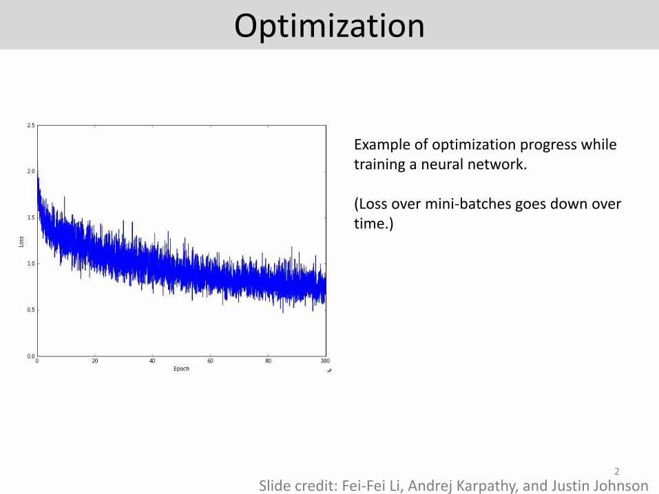
Example of optimization progress while training a neural network.

(Loss over mini-batches goes down over time.)

Slide credit: Fei-Fei Li, Andrej Karpathy, and Justin Johnson

Learning rate

3

The effects of step size (or “learning rate”)

Slide credit: Fei-Fei Li, Andrej Karpathy, and Justin Johnson

Multiple gradient update formulas

4

(image credits to Alec Radford)

The effects of different update form formulas

Slide credit: Fei-Fei Li, Andrej Karpathy, and Justin Johnson

Stochastic Gradient Descent (SGD)

• Update weights for each sample

• Minibatch SGD: Update weights for a small set of samples

5

𝐸 =1

2𝑦𝑛 − 𝑦𝑛 2 𝒘𝑖 𝑡 + 1 = 𝒘𝑖 𝑡 − 𝜖

𝜕𝐸𝑛

𝜕𝒘𝑖

𝐸 =1

2

𝑛∈𝐵

𝑦𝑛 − 𝑦𝑛 2 𝒘𝑖 𝑡 + 1 = 𝒘𝑖 𝑡 − 𝜖𝜕𝐸𝐵

𝜕𝒘𝑖

+ Fast, online− Sensitive to noise

+ Fast, online+ Robust to noise

Slide credit: Bohyung Han

Momentum

• Remember the previous direction

6

𝑣𝑖 𝑡 = 𝛼𝑣𝑖 𝑡 − 1 − 𝜖𝜕𝐸

𝜕𝑤𝑖(𝑡)

𝒘 𝑡 + 1 = 𝒘 𝑡 + 𝒗(𝑡)

+ Converge faster+ Avoid oscillation

Slide credit: Bohyung Han

Weight Decay

• Penalize the size of the weights

7

𝑤𝑖 𝑡 + 1 = 𝑤𝑖 𝑡 − 𝜖𝜕𝐶

𝜕𝑤𝑖= 𝑤𝑖 𝑡 − 𝜖

𝜕𝐸

𝜕𝑤𝑖− 𝜆𝑤𝑖

𝐶 = 𝐸 +1

2

𝑖

𝑤𝑖2

+ Improve generalization a lot!

Slide credit: Bohyung Han

Issues in Deep Neural Networks

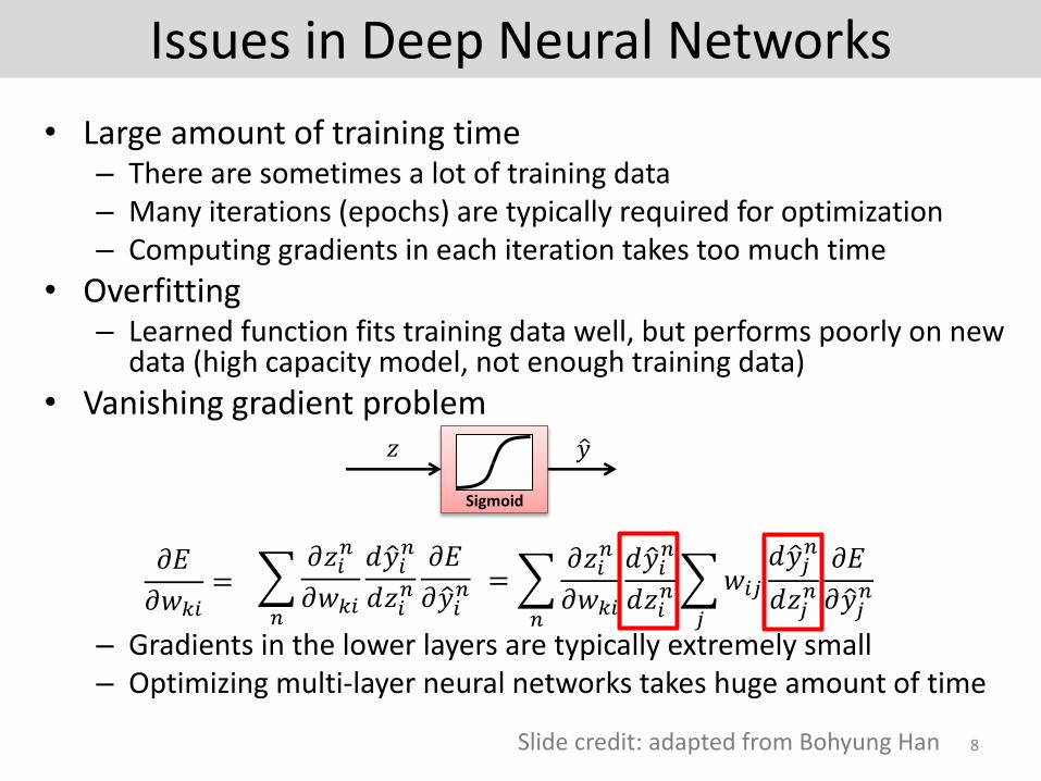
• Large amount of training time– There are sometimes a lot of training data– Many iterations (epochs) are typically required for optimization– Computing gradients in each iteration takes too much time

• Overfitting– Learned function fits training data well, but performs poorly on new

data (high capacity model, not enough training data)

• Vanishing gradient problem

– Gradients in the lower layers are typically extremely small– Optimizing multi-layer neural networks takes huge amount of time

8

𝜕𝐸

𝜕𝑤𝑘𝑖=

𝑛

𝜕𝑧𝑖𝑛

𝜕𝑤𝑘𝑖

𝑑 𝑦𝑖𝑛

𝑑𝑧𝑖𝑛

𝜕𝐸

𝜕 𝑦𝑖𝑛 =

𝑛

𝜕𝑧𝑖𝑛

𝜕𝑤𝑘𝑖

𝑑 𝑦𝑖𝑛

𝑑𝑧𝑖𝑛

𝑗

𝑤𝑖𝑗

𝑑 𝑦𝑗𝑛

𝑑𝑧𝑗𝑛

𝜕𝐸

𝜕 𝑦𝑗𝑛

Sigmoid

𝑧 𝑦

Slide credit: adapted from Bohyung Han

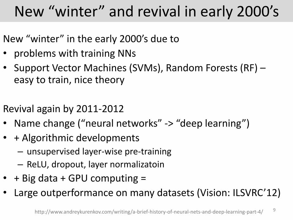
New “winter” and revival in early 2000’s

New “winter” in the early 2000’s due to

• problems with training NNs

• Support Vector Machines (SVMs), Random Forests (RF) –easy to train, nice theory

Revival again by 2011-2012

• Name change (“neural networks” -> “deep learning”)

• + Algorithmic developments– unsupervised layer-wise pre-training

– ReLU, dropout, layer normalizatoin

• + Big data + GPU computing =

• Large outperformance on many datasets (Vision: ILSVRC’12)

9http://www.andreykurenkov.com/writing/a-brief-history-of-neural-nets-and-deep-learning-part-4/

Big Data

• ImageNet Large Scale Visual Recognition Challenge– 1000 categories w/ 1000 images per category

– 1.2 million training images, 50,000 validation, 150,000 testing

10O. Russakovsky, J. Deng, H. Su, J. Krause, S. Satheesh, S. Ma, Z. Huang, A. Karpathy, A. Khosla,M. Bernstein, A. C. Berg and L. Fei-Fei. ImageNet Large Scale Visual Recognition Challenge. IJCV, 2015.

AlexNet Architecture

60 million parameters!Various tricks• ReLU nonlinearity• Overlapping pooling• Local response normalization• Dropout – set hidden neuron output to 0 with probability .5• Data augmentation• Training on GPUs

11Alex Krizhevsky, Ilya Sutskeyer, Geoffrey E. Hinton. ImageNet Classification with Deep Convolutional Neural Networks. NIPS, 2012.

Figure credit: Krizhevsky et al, NIPS 2012.

GPU Computing

• Big data and big models require lots of computational power

• GPUs

– thousands of cores for parallel operations

– multiple GPUs

– still took about 5-6 days to train AlexNet on two NVIDIA GTX 580 3GB GPUs (much faster today)

12

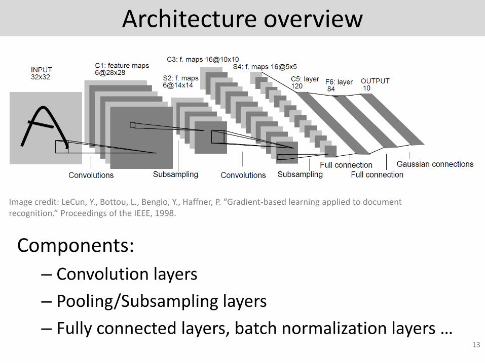
Architecture overview

Components:

– Convolution layers

– Pooling/Subsampling layers

– Fully connected layers, batch normalization layers …13

Image credit: LeCun, Y., Bottou, L., Bengio, Y., Haffner, P. “Gradient-based learning applied to document recognition.” Proceedings of the IEEE, 1998.

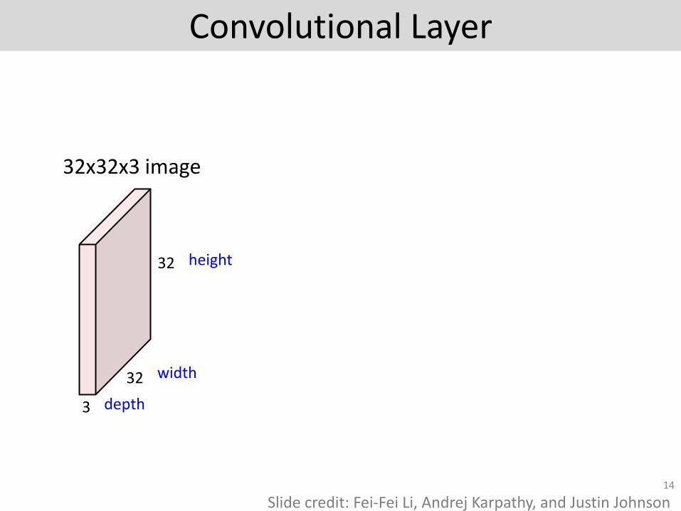
Convolutional Layer

14

32

32

3

32x32x3 image

width

height

depth

Slide credit: Fei-Fei Li, Andrej Karpathy, and Justin Johnson

11 Jan 2016

15

32

32

3

5x5x3 filter

32x32x3 image

Convolve the filter with the imagei.e. “slide over the image spatially, computing dot products”

Convolutional Layer

Slide credit: Fei-Fei Li, Andrej Karpathy, and Justin Johnson

11 Jan 2016

16

32

32

3

5x5x3 filter

32x32x3 image

Convolve the filter with the imagei.e. “slide over the image spatially, computing dot products”

Filters always extend the full depth of the input volume

Convolutional Layer

Slide credit: Fei-Fei Li, Andrej Karpathy, and Justin Johnson

11 Jan 2016

17

32

32

3

32x32x3 image5x5x3 filter

1 number: the result of taking a dot product between the filter and a small 5x5x3 chunk of the image(i.e. 5*5*3 = 75-dimensional dot product + bias)

Convolutional Layer

Slide credit: Fei-Fei Li, Andrej Karpathy, and Justin Johnson

11 Jan 2016

18

32

32

3

32x32x3 image5x5x3 filter

convolve (slide) over all spatial locations

activation map

1

28

28

Convolutional Layer

Slide credit: Fei-Fei Li, Andrej Karpathy, and Justin Johnson

11 Jan 2016

19

32

32

3

32x32x3 image5x5x3 filter

convolve (slide) over all spatial locations

activation maps

1

28

28

consider a second, green filter

Convolutional Layer

Slide credit: Fei-Fei Li, Andrej Karpathy, and Justin Johnson

11 Jan 2016

20

32

32

3

Convolution Layer

activation maps

6

28

28

For example, if we had 6 5x5 filters, we’ll get 6 separate activation maps:

We stack these up to get a “new image” of size 28x28x6!

Convolutional Layer

Slide credit: Fei-Fei Li, Andrej Karpathy, and Justin Johnson

11 Jan 2016

21

ConvNet is a sequence of Convolutional Layers, interspersed with activation functions

32

32

3

28

28

6

CONV,ReLUe.g. 6 5x5x3 filters

Convolutional Layer

Slide credit: Fei-Fei Li, Andrej Karpathy, and Justin Johnson

11 Jan 2016

22

ConvNet is a sequence of Convolutional Layers, interspersed with activation functions

32

32

3

CONV,ReLUe.g. 6 5x5x3 filters 28

28

6

CONV,ReLUe.g. 10 5x5x6 filters

CONV,ReLU

….

10

24

24

Convolutional Layer

Slide credit: Fei-Fei Li, Andrej Karpathy, and Justin Johnson

11 Jan 2016

23

The brain/neuron view of CONV Layer

32

32

3

32x32x3 image5x5x3 filter

1 number: the result of taking a dot product between the filter and this part of the image(i.e. 5*5*3 = 75-dimensional dot product)

Slide credit: Fei-Fei Li, Andrej Karpathy, and Justin Johnson

11 Jan 2016

24

The brain/neuron view of CONV Layer

32

32

3

32x32x3 image5x5x3 filter

1 number: the result of taking a dot product between the filter and this part of the image(i.e. 5*5*3 = 75-dimensional dot product)

It’s just a neuron with local connectivity...

Slide credit: Fei-Fei Li, Andrej Karpathy, and Justin Johnson

11 Jan 2016

25

The brain/neuron view of CONV Layer

32

32

3

An activation map is a 28x28 sheet of neuron outputs:1. Each is connected to a small region in the input2. All of them share parameters

“5x5 filter” -> “5x5 receptive field for each neuron”

28

28

Slide credit: Fei-Fei Li, Andrej Karpathy, and Justin Johnson

11 Jan 2016

26

The brain/neuron view of CONV Layer

32

32

3

28

28

E.g. with 5 filters,CONV layer consists of neurons arranged in a 3D grid(28x28x5)

There will be 5 different neurons all looking at the same region in the input volume

5

Slide credit: Fei-Fei Li, Andrej Karpathy, and Justin Johnson

11 Jan 2016

27

- makes the representations smaller and more manageable - operates over each activation map independently:

Pooling Layer

Slide credit: Fei-Fei Li, Andrej Karpathy, and Justin Johnson

11 Jan 2016

28

1 1 2 4

5 6 7 8

3 2 1 0

1 2 3 4

Single depth slice

x

y

max pool with 2x2 filters and stride 2 6 8

3 4

MAX POOLING

Pooling Layer

Slide credit: Fei-Fei Li, Andrej Karpathy, and Justin Johnson

Many more details

• Data preprocessing

• Initialization

• Learning rate

• Batch normalization layer

• ReLU, pReLU, other activation functions

• …

29

11 Jan 2016

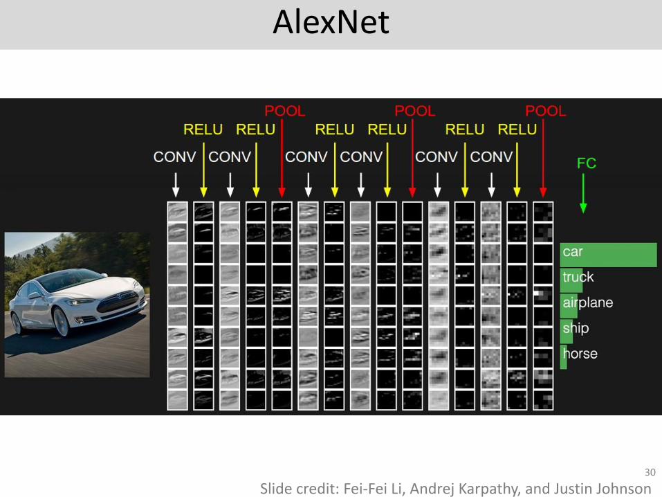
30

AlexNet

Slide credit: Fei-Fei Li, Andrej Karpathy, and Justin Johnson

11 Jan 2016

31

[From recent Yann LeCun slides]

Convolutional filter visualization

Slide credit: Fei-Fei Li, Andrej Karpathy, and Justin Johnson

11 Jan 2016

32

[From recent Yann LeCun slides]

Convolutional filter visualization

Slide credit: Fei-Fei Li, Andrej Karpathy, and Justin Johnson

11 Jan 2016

33

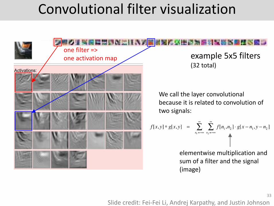
example 5x5 filters(32 total)

We call the layer convolutional because it is related to convolution of two signals:

elementwise multiplication and sum of a filter and the signal (image)

one filter => one activation map

Convolutional filter visualization

Slide credit: Fei-Fei Li, Andrej Karpathy, and Justin Johnson

11 Jan 2016

34

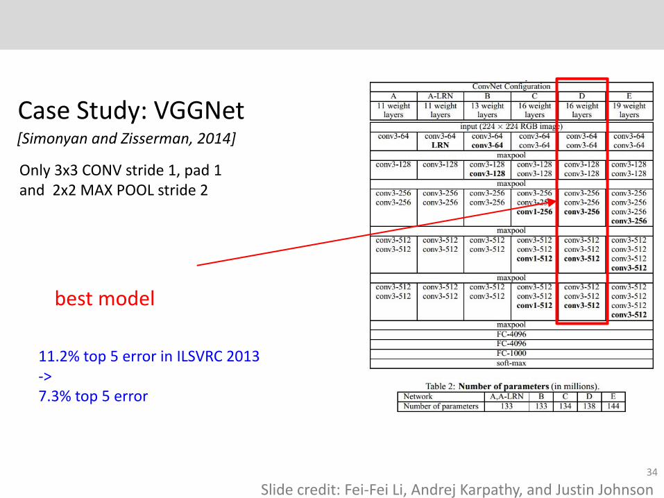
Case Study: VGGNet[Simonyan and Zisserman, 2014]

best model

Only 3x3 CONV stride 1, pad 1and 2x2 MAX POOL stride 2

11.2% top 5 error in ILSVRC 2013->7.3% top 5 error

Slide credit: Fei-Fei Li, Andrej Karpathy, and Justin Johnson

11 Jan 2016

35

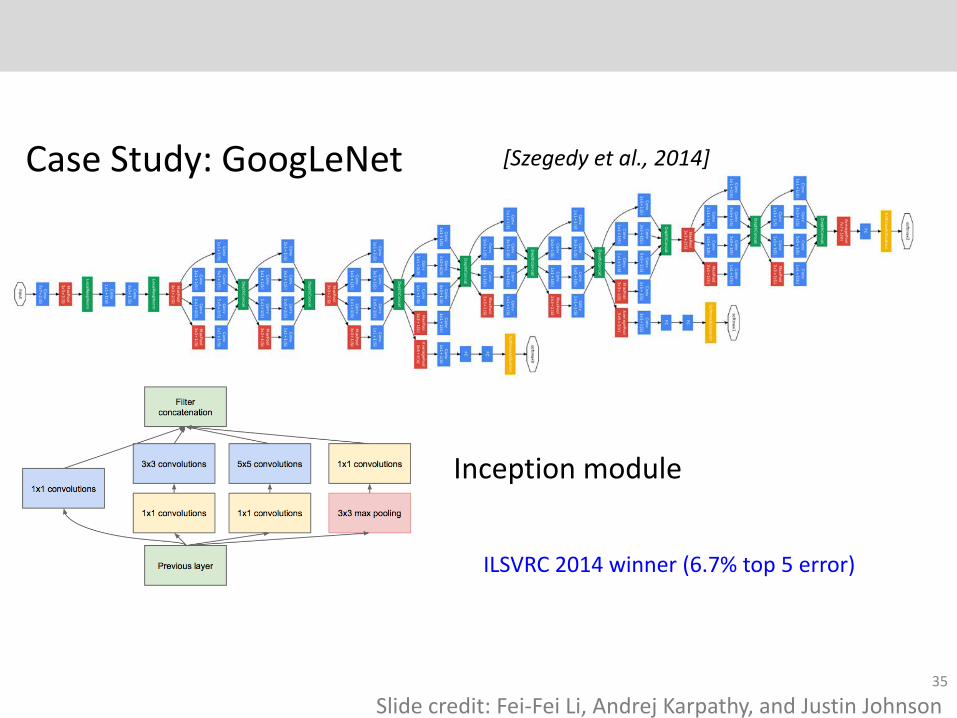
Case Study: GoogLeNet [Szegedy et al., 2014]

Inception module

ILSVRC 2014 winner (6.7% top 5 error)

Slide credit: Fei-Fei Li, Andrej Karpathy, and Justin Johnson

11 Jan 2016

36

Case Study: ResNet [He et al., 2015]

Slide credit: Fei-Fei Li, Andrej Karpathy, and Justin Johnson

Questions?

References (& great tutorials):

http://cs231n.stanford.edu/syllabus.html

http://cs231n.github.io/neural-networks-1/

http://cvlab.postech.ac.kr/~bhhan/class/cse703r_2016s.html

37

Unsupervised Neural Networks

Autoencoders• Encode then decode the same

input• No supervision needed

(Restricted) Boltzman Machines (RBMs)• Stochastic networks that can learn

representations • Restricted version: neurons must

form bipartite graph

38

input x

hidden layer

output x’

input x

hidden layer

H. Bourlard and Y. Kamp. 1988. Auto-association by multilayer perceptrons and singular value decomposition.Biol. Cybern. 59, 4-5 (September 1988), 291-294.

Ackley, David H; Hinton Geoffrey E; Sejnowski, Terrence J, "A learning algorithm for Boltzmann machines", Cognitive science, Elsevier, 1985.Smolensky, Paul. "Chapter 6: Information Processing in Dynamical Systems: Foundations of Harmony Theory.” In Parallel Distributed Processing: Explorations in the Microstructure of Cognition, Volume 1: Foundations, 1986.

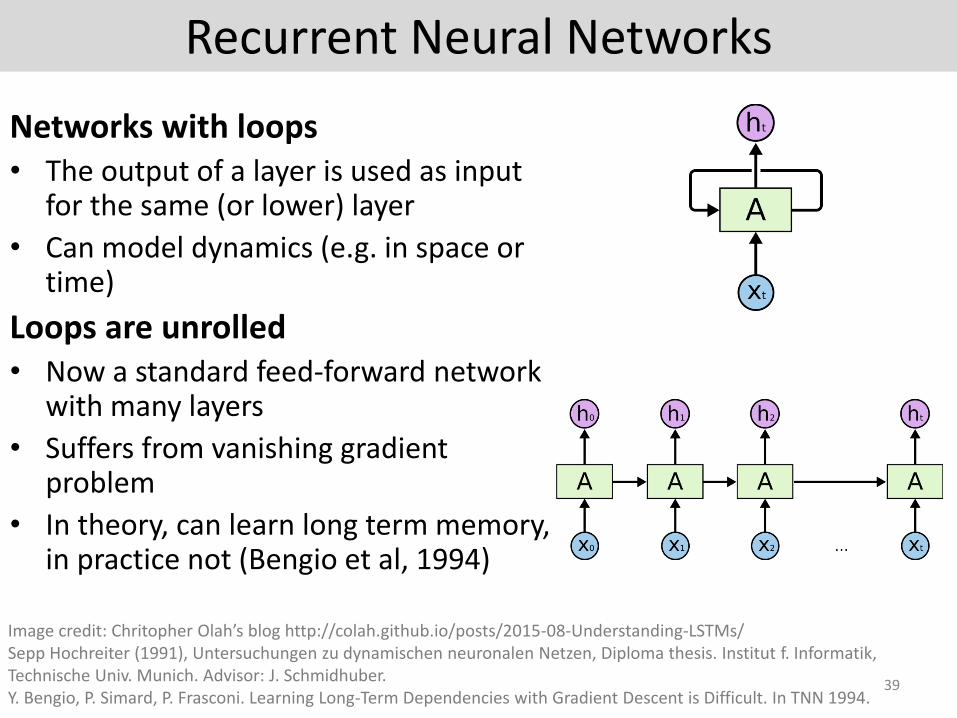
Recurrent Neural Networks

Networks with loops• The output of a layer is used as input

for the same (or lower) layer

• Can model dynamics (e.g. in space or time)

Loops are unrolled• Now a standard feed-forward network

with many layers

• Suffers from vanishing gradient problem

• In theory, can learn long term memory, in practice not (Bengio et al, 1994)

39

Image credit: Chritopher Olah’s blog http://colah.github.io/posts/2015-08-Understanding-LSTMs/Sepp Hochreiter (1991), Untersuchungen zu dynamischen neuronalen Netzen, Diploma thesis. Institut f. Informatik, Technische Univ. Munich. Advisor: J. Schmidhuber.Y. Bengio, P. Simard, P. Frasconi. Learning Long-Term Dependencies with Gradient Descent is Difficult. In TNN 1994.

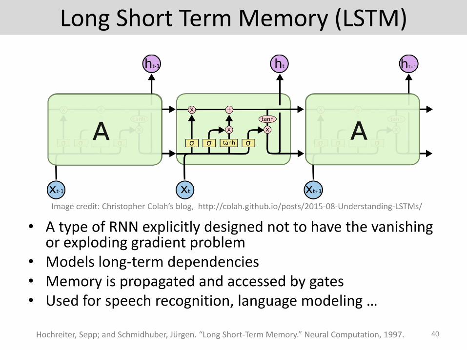
Long Short Term Memory (LSTM)

• A type of RNN explicitly designed not to have the vanishing or exploding gradient problem

• Models long-term dependencies• Memory is propagated and accessed by gates• Used for speech recognition, language modeling …

40Hochreiter, Sepp; and Schmidhuber, Jürgen. “Long Short-Term Memory.” Neural Computation, 1997.

Image credit: Christopher Colah’s blog, http://colah.github.io/posts/2015-08-Understanding-LSTMs/

Image Classification Performance

41

Image Classification Top-5 Errors (%)Slide credit: Bohyung HanFigure from: K. He, X. Zhang, S. Ren, J. Sun. “Deep Residual Learning

for Image Recognition”. arXiv 2015. (slides)