20
Growth and Convergence in a Two-Region Model of Uni�ed Germany
Michael Funke�
Department of EconomicsHamburg UniversityVon Melle Park 520146 Hamburg
Holger StrulikDepartment of Applied Economics
University of CambridgeSidgwick Avenue
Cambridge CB3 9DEU.K.
Cambridge/Hamburg, September 1999
Abstract
The paper sets up a two-region endogenous growth model to discuss growth and regionalconvergence of uni�ed Germany. It emphasises the role of private and public capital ac-cumulation during the developing process. The theoretical part derives �scal policy ruleswhich establish convergence of regional output per capital and convergence of regional hu-man wealth. To assess the speed of convergence the model is calibrated with German data.Given a �scal policy rule that is consistent with the data on government spending in Eastand West Germany after uni�cation the model suggests that East Germany will reach eightypercent of West Germany's income per capita between 20 and 30 years after uni�cation andthat actual transfers are approximately su�cient to equalise regional human wealth. Theresults are compared with an extension of the model that includes wage setting behaviourand unemployment in the eastern region.
Keywords: German Uni�cation, Regional Convergence, Government SpendingJEL classi�cation: O41, O52, H31, H40
�We would like to thank Andreas Pick for helpful comments. This research was supported through a MarieCurie Research Fellowship of the European Commission.
1 Introduction
On 2 July 1990, East and West Germany became economically united through a commoncurrency. Ten years after, the e�ects of German reunifcation continue to reverberate inGermany. The abrupt exposure of the structurally-weak East German economy to compe-tition from the world markets in 1990 resulted in a strong decline of economic activity inthe �ve new federal states (Bundesl�ander). The industrial depression that followed the shockof uni�cation ended in 1991 but on the other hand there is no Wirtschaftswunder. WestGermany's post-war recovery was buttressed by an undervalued Deutschmark and by lowwages, both of which boosted exports. Eastern Germany has neither advantage; instead itis su�ering from two policy blunders. Uni�cation saddled the region with a currency whosevalue re ected western Germany's highly productive industry. And employers worsened thathandicap by agreeing to raise eastern German wages to western levels far more rapidly thanthe productivity gap could be closed. Given this situation both state governments and theTreuhandanstalt, the agency charged with privatising eastern German industry, have rescued\industrial cores" on the theory that new businesses will spring up only where some industrystill survives.1 But the price of such rescues has been very high. After all, more than DM 1trillion of public money has been pumped into the East since unity. The annual bill is stillrunning at close to a net DM 150 billion, in part �nanced by a \solidarity" income-tax levy.Despite all that, the eastern jobless rate is still twice that of the West, productivity is a goodthird lower, exports remain weak. This is in sharp contrast to Helmut Kohl's now notoriousclaim in 1990 that there would be \ ourishing landscapes" in the East within �ve years.Given these developments, the paper deals with the long- term prospects of the East Germaneconomy. We consider the impact of �scal policy in a two-region endogenous growth modelwhich emphasizes the role of private and public capital accumulation during the transitionprocess.
The theoretical model can be understood as an extension of Ono and Shibata's (1992)two{country model with public capital accumulation and interregional �scal transfers. Em-phasising the role of factor accumulation during the catching-up process, economic growth isdriven by the accumulation of private and public capital. Therefore, the model can also beunderstood as a two{country (region) version of Barro's (1990) model on government spend-ing and economic growth. In contrast to Barro (1990), however, we will regard productivegovernment expenditure as a ow variable that extends the stock of available public capital.Therefore, the model exhibits transitional dynamics and �scal policy crucially determines thespeed of (regional) convergence. The analysis of regional di�erences in �nancial and humanwealth uses ideas recently developed in Caselli and Ventura (1999), and the solution techniqueemploys the method of backward integration developed in Brunner and Strulik (1998).
The remainder is structured in six sections. Section 2 lays out the basic theoreticalframework. Section 3 discusses interregional and economy-wide dynamics. Section 4 dealswith �scal redistribution. Section 5 presents numerical solutions for a calibrated model whilesection 6 analyses an extended model allowing for unemployment. Section 7 provides someconclusions and discusses limitations of the approach followed in the paper.
1The importance of 'Industrial Cores' for regional growth has recently been modelled in Englmann undWalz (1995).
1
2 The Model
2.1 Firms
In each region there exists a large number of identical �rms. They operate under perfectcompetition and employ private capital ki and labour li to produce an output yi with con-stant returns to scale in privately provided factors. Malleable output can be either used forconsumption, private investment, or public expenditure and the production function has theCobb-Douglas form:
yi = Aiki�li
1��; i = W;E; 0 < � < 1 : (1)
The productivity parameter Ai is exogenous to the �rm but partly determined by productivegovernment spending. The price of goods is normalised to one. Firms control labour inputsli and investment Ii. With depreciation rate � > 0 the capital stock develops according to
_ki = Ii � �ki : (2)
Firms have to pay a corporate tax on cash ow with constant rate � . They maximise thepresent value of their intertemporal net pro�t ow Vi(0) =
R1
0exp[��ri(t)t]f(1��)[yi�wili]�
Iigdt subject to (2), where wi denotes the wage rate and
�ri(t) =1
t
Z t
0
ri(s)ds (3)
is the average interest rate between times 0 and t. According to the �rst order conditions,factor prices are given by
wi = (1� �)Ai(Ki=Li)� ; and (4)
ri = (1� �)�Ai(Ki=Li)��1 � � : (5)
In writing (4) and (5) we have used the fact that all �rms are identical and hence choose acapital labour ratio that equals the capital labour ratio of their region, ki=li = Ki=Li.
2.2 Government Behaviour
The government taxes corporate income and individual income with a single rate. To avoiddouble taxation individual interest earnings are tax exempt. Tax earnings are at least partlyspent on the accumulation of productive public capital Gi. The remainder is spend on transferpayments within a region, Zi, and intra-regional transfers. The government runs a balancedbudget which can be written as
�(YW + YE) = _GW � �GW + _GE � �GE + ZW + ZE ; (6)
where � is the depreciation rate of public capital. The analysis simpli�es greatly if we assumea two-step procedure in government budgeting. In the �rst step the government decidesseparately for each region how to spend regional tax earnings. In the second step it performsinterregional redistribution according to a system of �scal equalisation (L�ander�nanzaus-gleich). With 0 � qi � 1 denoting the share spent on productive services and x denoting
2
the fraction of Western tax earning transferred to the East, government behaviour can besummarised as
_Gi = qi�Yi � �Gi ;
ZW = (1� qW � x)�YW ; (7)
ZE = (1� qE)�YE + x�YW :
We follow Barro (1990) in assuming decreasing returns of infrastructure so that the macro-economy exhibits constant returns to scale in private and public capital. Since the regionsdi�er in size their infrastructure has to be scaled by population size to eliminate unwantedscale e�ects. The regional factor productivity Ai is then given by
Ai = A(Gi=Li)1�� ; A > 0 ; (8)
where A denotes a general productivity parameter which is assumed to be identical in bothregions.2
2.3 Households
Each region is populated by a large number of households, numbered j = 1; : : : ; LW andj = 1; 2; : : : ; LE, respectively. Each household supplies one unit of labour inelastically andmaximises utility from intertemporal consumption
U ji =
Z1
0
cji1��
� 1
1� �e��tdt ; (9)
subject to his budget constraint
cji + _aji = riaji + (1� �)wj
i + zji ; (10)
where � denotes the time preference rate, and ��1 < 1 is the intertemporal elasticity ofsubstitution. Individuals may di�er in their initial endowment of �nancial wealth aji (0) and
in their received transfers, zji . The heterogeneity in wealth across both region may explainthe existence of intra-regional transfers. From the �rst order conditions of the correspondingcurrent value Hamiltonian we obtain the Ramsey rule
_ci=ci = [ri � �]=� ; (11)
which applies to all consumers independently from wealth or provenance.
2.4 A Fiscal Policy Rule for Economic Convergence
Uni�cation induces a spontaneous equalisation of regional interest rates through capital move-ments towards the region with the higher net marginal product of private capital. Applyingthe interest parity on (5) and using (8) yields
� � yE=yW =KE=LE
KW =LW
=GE
GW
1
�; where (12)
� � LE=LW : (13)
2Equation (8) introduces a mechanism through which infrastructure provided by the government a�ectsthe productivity of privately owned factors. The empirical paper by Duggal et al. (1999) provides a rationalefor the chosen speci�cation.
3
Equations (12) and (13) introduce two measures of regional di�erences. The �rst one, �,measures the relative backwardness of the eastern region in terms of eastern income percapita relative to western income per capita. The second one, �, is a scale variable thatcontrols for the size of the regional work force.
Equation (12) displays the basic mechanism of the model: Interregional mobile privatecapital ties down the East's relative income per capita to its relative stock of infrastructureper capita. If, for example, the pre-uni�cation levels of private and public capital per capitawere KE=LE = 0:4KW=LW and GE=LE = 0:5GW=LW , then uni�cation would lead to aspontaneous reallocation of private capital from the West to the East so that KE=LE =0:5KW=LW and hence � = 0:5. For simplicity we assume that any possible di�erence in theregion's relative endowment with private and public capital are equalised by private capital ows at uni�cation time so that the starting point of the analysis is uniquely determined bythe regional distribution of infrastructure.3
Consider now a government that simply adopts the \successful" western policy in theeastern part of the country , i.e. qE = qW . After insertion of (8) and (12) into (7) we obtain
� �_�
�= (qE � qW )�A
�GW
KW
���
: (14)
Hence, there will never be convergence if the richer region's �scal policy is imposed upon thepoorer region. In conclusion infrastructure spending in the poorer region must be temporar-ily higher to attract private capital. The following proposition shows the policy rule thatestablishes income convergence between the East and the West.
Proposition 1 Consider the two-region endogenous growth model as described above. Let
the eastern region be initially backward in terms of per capita income relative to the western
region. Then the unique set of monotonous �scal policy functions that establishes economic
convergence is determined by
qE = [f(�) + 1] qW ; f 0 < 0; f(1) = 0 : (15)
The proof inserts (15) into (14). In the remainder of the paper we assume that the governmenthas the objective to realise regional convergence and, therefore, adopts a policy rule from theset of feasible functions (15). Note that the policy does not depend on time but on thestate of the system, namely the distance of the East from its western counterpart so that itconstitutes a time consistent credible policy.
3 Economic Convergence
3.1 Interregional and Economy-Wide Dynamics
From the country-wide perspective any income which is not spent on infrastructure accu-mulation is spend on either consumption, C, or private capital accumulation, _K. Hence theeconomy-wide private capital stock
K = KW +KE = (1 + ��)KW (16)
3The instantaneous relocation of private capital occurs because the model does not contain any adjustmentcosts.
4
develops according to
_K = (1� �qW )A
�GW
KW
�1��
KW + (1� �qE)A
�GE
KE
�1��
KE � C � �K (17)
Let the economy-wide consumption-capital ratio be de�ned as � � C=K and western in-frastructure per unit of total private capital as gW � GW =K. Using (12) , (15), and (16)equation (17) can be rewritten as
K � _K=K = f1 + �� � �qW [1 + �(f(�) + 1)]gAg1��W (1 + ��)�� � � � � : (18)
Employing (5) and (10) we obtain in the same way
� � _C=C � K =1
�
�(1� �)�Ag1��
W(1 + ��)1�� � (� + �)
�� K ; (19)
and (7) and (14) can be rewritten as
gW � _GW =GW � K = qW �Ag��W (1 + ��)�� � � � K ; (20)
� = f(�)qW �Ag��W (1 + ��)�� : (21)
With equations (18) { (21) the economy is described by a three dimensional di�erentialequation system in �, gW and �.
3.2 Equilibrium Analysis
At the equilibrium we have �? = 1 from (21). After insertion of (20) into (19) the equilibriumvalue of gW is determined by the implicit function
0 = F (gW ) =�(1� �)�Ag1��W (1 + �)1�� � (� + �)
�=� � qW �Ag��W (1 + �)�� + � : (22)
Since F 0 > 0 for all positive gW and limgW!0 F (gW ) = �1 and limgW!1 F (gW ) = 1 aunique equilibrium gW
? exists. At this equilibrium �? is obtained as
�? = (1 + �)1��Ag?W1�� [1� �qW � (1� �)�=�] + (� + �)=�� � (23)
from (18) and (19). Generally, (22) can only be solved numerically. It is, however, usefulto consider for a moment the special parameterisation � = (� � 1)� for which gW
? can beobtained analytically as
gW? =
�qW �
(1� �)�(1 + �): (24)
After insertion into (19) the equilibrium growth rate of the economy is calculated as
C = [�(1� �)=�]�A(qW �)1�� � � : (25)
By derivation with respect to � it can be veri�ed that the long-run growth maximising taxrate is � = 1 � �.4 Hence, Barro's (1990) �nding that the optimal income tax rate equals
4The empirical literature on economic growth, dominated by cross-country regressions and tests of incomeconvergence across countries, has recently been enriched by studies that provide direct tests of endogenousgrowth models utilising time series data. Kocherlakota and Yi (1997) have recently provided empirical evidencefor the U.S. and the U.K. that permanent changes in �scal policy can have permanent e�ects on growth rateseven though the growth rate itself appears stable over time.
5
the production elasticity of infrastructure is replicated in the two-region growth model withinter- and intra-regional transfers.
The Jacobian determinant at the steady-state is computed as det J = @ �=@�[@ gW =@gW�@ �=@gW ] with
@ �@�
= f 0(�)(1 + �)��qW �Ag��W < 0 ;
@ gW@gW
�@ �@gW
= ��(1 + �)��qW �Ag���1W
� (1� �)(1� �)(1 + �)1���Ag��W
=� < 0
so that the equilibrium is a saddlepoint. The eigenvalues are
�1 =@ �@�
< 0 and
�2;3 =
�1 +
@ gW@gW
�q(1 + @ gW =@gW )2 � 4(@ gW=@gW � @ �=@gW )
�=2 :
Since @ gW =@gW �@ �=@gW < 0 all eigenvalues are real so that the adjustment path towardsthe equilibrium is monotonous. For reasonable parameterisations of the model it turns outthat two eigenvalues are negative, so that the stable manifold is two-dimensional.
At the steady{state consumption, public capital, and private capital grow with identi-cal rates economy-wide, which can be seen from (19) and (20), as well as in its regionalcomponents, which can be seen from (11) and (12).
4 Interregional Income Redistribution: The Solidarity Pact
The problem of regional convergence has been solved independently from the existence ofinterregional income redistribution. So far, however, we have only discussed the convergenceof regional income produced but not the problem of convergence of income earned, i.e. the con-vergence of regional wealth and regional consumption. For that purpose let us now comparethe average individual in the East with its counterpart in the West. From (7) we see that theaverage western individual receives income transfers zW = ZW =LW = (1� qW � x)�YW =LW
and the average eastern individual receives zE = (1� qE)�YE=LE + x�YW =LE . With use of(4) and the de�nitions of � and � their budget constraints (10) can be written as
_aW = [1� �(1� �)� qW � � x� ] yW � cW + raW ; (26)
_aE =h(1� �(1� �))� � qE�� +
x�
�
iyW � cE + raE : (27)
After integrating (26) and (27) and substituting the integrated version of (11) we arrive aftersome amount of algebra at
cE(t)
cW (t)=
cE(0)
cW (0)=
aE(0) +R1
0
�(1� �(1� �))� � qE�� +
x��
�yW e�
Rt
0�rdvdt
aW (0) +R1
0[1� �(1� �)� qW � � x� ] yW e�
Rt
0�rdvdt
(28)
The �rst sign of equality originates from the fact that all individuals choose the same in-tertemporal allocation of consumption. Regional levels of consumption converge if the righthand side of the equation equals one.
Let us �rst consider a government that attempts to realise convergence of consumption andthe hypothetical case of spontaneous economic convergence at uni�cation time. In this casethe integrals in (28) are identical for x = 0 but even then the eastern individual would be worse
6
o� if he brings along a lower initial endowment of �nancial wealth. The only possibility toproduce convergence of consumption is to partly expropriate the western individual. Suppose,for example, that KE=LE equals 0:5KW=LE before uni�cation and that all eastern capital isowned by the eastern population so that the average eastern individual is half as rich in termsof �nancial wealth as his western counterpart. If the westerner donates half of his wealth tothe easterner than aE(0) = aW (0) and cE = cW for all t.
This leads to the following conclusion. While equating the ai's means to compensate theeastern individual for the bad performance of his economy before uni�cation, equating theintegrals means to compensate the eastern individual for the relatively bad performance of hisnative region after uni�cation. We have emphasised this distinction to motivate the followingassumption about government behaviour. The government does not take responsibility forthe bad performance of the eastern region before uni�cation but takes responsibility for thewell being of eastern individuals after uni�cation. Formally this means that the governmenttries to equalize consumption levels of individuals with initially equal �nancial wealth, i.e. ittries to equalize consumption levels as if the eastern individuals are initially equally equippedwith �nancial wealth.
Assuming that the government compensates only disadvantages which originate fromliving in the poorer region after uni�cation is of course a highly normative judgement but ithas a very useful implication.5 Since equating the integrals means equating human wealth orintertemporal non-�nancial income the income transfer policy prevents regional migration.Although, this applies in a strict sense only to the average eastern individual it is generallypossible to construct a deliberate spending policy that realises the result for all individualsonce their speci�c individual economic situation is known. In turn, any policy that tries tocompensate for di�erent initial ai may lead to migration of western individuals to the East inorder to receive transfers that make them at least partly o� for their initial loss in �nancialwealth.6
After equating the integrals and inserting the income convergence policy (15) we obtainthe income transfer policy as
x = f[1� �(1� �)� qW � ] (1� �) + f(�)qW ��g
��
�(�+ 1)
�: (29)
The magnitude of transfers depends on the chosen policy to achieve economic convergence.The policy rule implies that transfers will have an end when income per worker has converged,x = 0 for � = 1. Transfers decline with increasing degree of economic convergence, @x=@� < 0,and will be the lower the smaller the poorer region.
5 Model Calibration and Solution Technique
The model is calibrated so that its steady-state solution matches West Germany's pre-uni�cation's performance. Unless otherwise speci�ed the data is taken from StatistischesBundesamt (1997). From the Eastern and Western population size we calculate � = 0:25.We set � = 0:5 from Western Germany's government share and qW = 0:1 from the average
5The assumption seems reasonable since the German mainstream parties are overwhelming dominated bywestern politicians.
6Equating the integrals equates the intertemporal stream of wages and governmental transfers in the Eastand West. Equal human wealth, however, does not necessarily rule out the possibility of wage setting behavioursince this may be motivated by initial di�erences in �nancial wealth or any other reason beyond the scope ofthe model.
7
pre-uni�cation value of West Germany's infrastructure share in government spending. Fromnumerous other calibration studies we adopt � = 0:02.
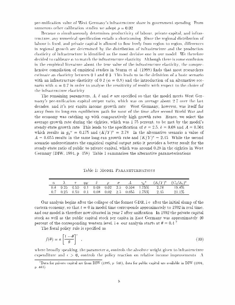
Because � simultaneously determines productivity of labour, private capital, and infras-tructure, any numerical speci�cation entails a shortcoming. Since the regional distribution oflabour is �xed, and private capital is allowed to ow freely from region to region, di�erencesin regional growth are determined by the distribution of infrastructure and the productionelasticity of infrastructure is identi�ed as the most decisive one in our model. We thereforedecided to calibrate � to match the infrastructure elasticity. Although there is some confusionin the empirical literature about the true value of the infrastructure elasticity, the compre-hensive compilation of empirical studies in Sturm et al. (1998) �nds that most researchersestimate an elasticity between 0.1 and 0.3. This leads us to the de�nition of a basic scenariowith an infrastructure elasticity of 0.2 (� = 0:8) and the introduction of an alternative sce-nario with � = 0:7 in order to analyse the sensitivity of results with respect to the choice ofthe infrastructure elasticity.
The remaining parameters, A, � and � are speci�ed so that the model meets West Ger-many's pre-uni�cation capital output ratio, which was on average about 2.7 over the lastdecades, and it's per capita income growth rate. West Germany, however, was itself faraway from its long-run equilibrium path for most of the time after second World War andthe economy was catching up with comparatively high growth rates. Hence, we select theaverage growth rate during the eighties, which was 1.75 percent, to be met by the model'ssteady-state growth rate. This leads to the speci�cation of � = 2:5, � = 0:08 and A = 0:504which results in gy
? = 0:175 and (K=Y )? = 2:78. In the alternative scenario a value ofA = 0:655 results in the same long-run growth rate and (K=Y )? = 2:45. While the secondscenario underestimates the empirical capital output ratio it provides a better result for thesteady-state ratio of public to private capital, which was around 0:28 in the eighties in WestGermany (DIW, 1994, p. 458). Table 1 summarises the alternative parameterisations.
Table 1: Model Parameterisations
� � � qW � � � A y? (K=Y )? (Gi=Ki)?
0:8 0:25 0:50 0:1 0:08 0:02 2:5 0:504 1:75% 2:78 18:4%0:7 0:25 0:50 0:1 0:08 0:02 2:5 0:655 1:75% 2:45 21:1%
Our analysis begins after the collapse of the former GDR, i.e. after the initial slump of theeastern economy, so that t = 0 in model time corresponds approximately to 1992 in real time,and our model is therefore now situated in year 7 after uni�cation. In 1992 the private capitalstock as well as the public capital stock per capita in East Germany was approximately 40percent of the corresponding western level, i.e. our analysis starts at � = 0:4.7
The �scal policy rule is speci�ed as
f(�) = a
�1� �
�
��; (30)
where broadly speaking, the parameter a, controls the absolute weight given to infrastructureexpenditure and � > 0, controls the policy reaction on relative income improvements. A
7Data for private capital are from DIW (1995, p. 540), data for public capital are available in DIW (1994,p. 461).
8
higher � speci�es a more reluctant �scal policy at higher �'s, i.e when the eastern economyhas already caught up parts of its initial backwardness. We set � = 1 in the basic scenarioand consider an alternative policy with � = 1:5. The choice of � and the actual governmentspending policy at t = 0 determine the value of a, so that (30) meets the actual �scal policyafter uni�cation.
Relating the data on government investment in DIW (1995, p. 537) to eastern GDP in thecorresponding years we calculate infrastructure investment in eastern Germany of between9 and 10 percent of East Germany's GDP in the early nineties, so that 0:1 = �qE impliesqE(0) = 0:2 and a = 2=3 for the basic �scal policy rule and a = 0:5443 for � = 1:5.
After inserting (30) and the parameters from Table 1 in (29) the initial share of transfersto the East in western tax earnings is obtained as
x(0) = f[1� 0:8 � (1� 0:5) � 0:1 � 0:4] [1� 0:4] + 0:8 � 0:1 � 0:4 � 1g
�0:25
1:25 � 0:5
�= 13:7% :
The existence of a two-dimensional stable manifold provides us with a further advantagein modelling uni�cation. It enables us to specify a second initial condition, which identi�esa unique adjustment path from the feasible set of trajectories on the manifold. Under theassumption that West Germany was approximately developing on its steady-state growthpath its public to private capital ratio before uni�cation is implicitly determined by thesteady-state after uni�cation through GW (0)=KW (0) = gW
?(1 + �) and hence gW (0) =gW
?(1 + �)=(1+ �(0)�).We solve the numerical problem with the method of backward integration. The general
method is described in Brunner and Strulik (1998) and the appendix of this paper showsits application to the two-region model. The main feature of the method is that it reveals{ besides of arbitrarily small discretisation errors { the exact adjustment path rather thanapproximations. After having obtained the adjustment path we use (1), (8), (13), and (16)to recalculate regional growth rates as
KW= K � �
��
1 + ��;
KE= KW
+ � ;
gE = � + gW ; (31)
YW = (1� �) gW + KW;
YE = (1� �) gE + KE:
5.1 Results
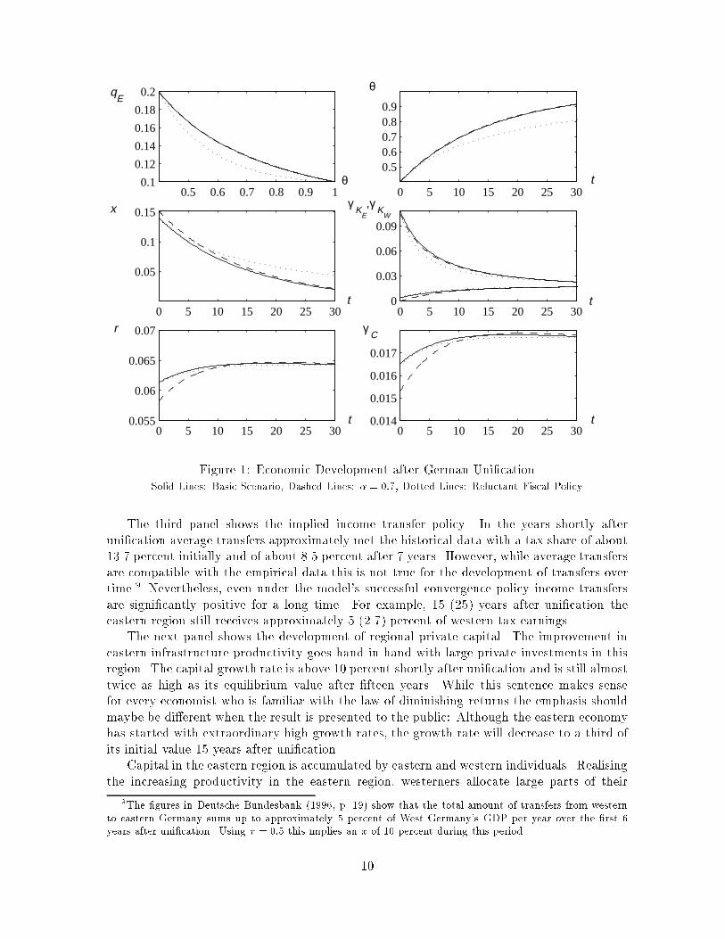
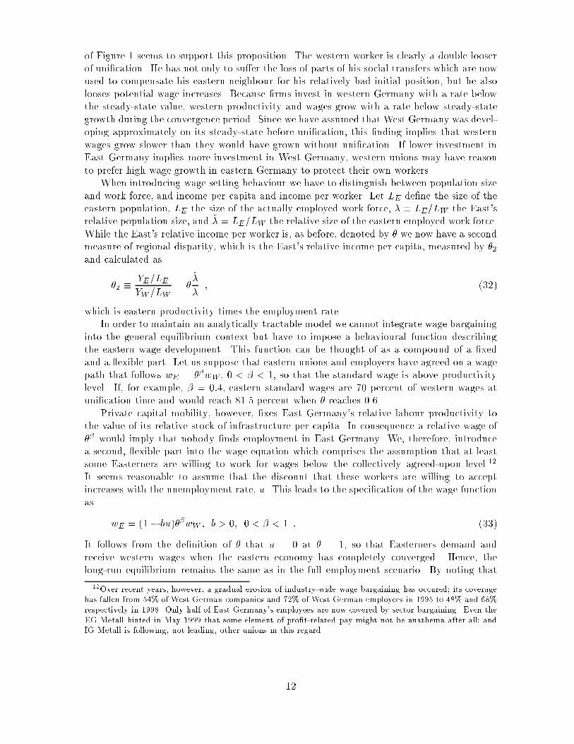
Eastern and western Germany's development and convergence in the basic scenario is de-scribed by the solid lines in Figure 1. The �rst panel on the left shows the �scal policy qE(�)as implied by (30). The other panels show the resulting time paths for several interestingvariables. The main variable of interest, the degree of backwardness of the eastern region isshown in the �rst panel on the right hand side. In the basic scenario half of the initial gapbetween East and West is closed after about 10 years after uni�cation and after about 30years the eastern region shows 90 percent of the productivity of its western counterpart.8
Bearing in mind that the starting point in real time was 1992 the eastern economy hasnow, 1999, reached 63 percent of West Germany's productivity level.
8This prediction is similar to the simulation results in Burda and Funke (1995). On the contrary Barro(1991), Barro and Sala-i-Martin (1991), Dornbusch and Wolf (1992), and Hughes Hallet and Ma (1993) havepredicted that convergence of living standards will take much longer.
9
0.5 0.6 0.7 0.8 0.9 10.1
0.12
0.14
0.16
0.18
0.2
0 5 10 15 20 25 30
0.50.60.70.80.9
0 5 10 15 20 25 30
0.05
0.1
0.15
0 5 10 15 20 25 300
0.03
0.06
0.09
0 5 10 15 20 25 300.055
0.06
0.065
0.07
0 5 10 15 20 25 300.014
0.015
0.016
0.017
qE
θ
θ
x γ K
E
,γ K
W
r γ C
t
t t
t t
Figure 1: Economic Development after German Uni�cationSolid Lines: Basic Scenario, Dashed Lines: � = 0:7, Dotted Lines: Reluctant Fiscal Policy
The third panel shows the implied income transfer policy. In the years shortly afteruni�cation average transfers approximately met the historical data with a tax share of about13.7 percent initially and of about 8.5 percent after 7 years. However, while average transfersare compatible with the empirical data this is not true for the development of transfers overtime.9 Nevertheless, even under the model's successful convergence policy income transfersare signi�cantly positive for a long time. For example, 15 (25) years after uni�cation theeastern region still receives approximately 5 (2.7) percent of western tax earnings.
The next panel shows the development of regional private capital. The improvement ineastern infrastructure productivity goes hand in hand with large private investments in thisregion. The capital growth rate is above 10 percent shortly after uni�cation and is still almosttwice as high as its equilibrium value after �fteen years. While this sentence makes sensefor every economist who is familiar with the law of diminishing returns the emphasis shouldmaybe be di�erent when the result is presented to the public: Although the eastern economyhas started with extraordinary high growth rates, the growth rate will decrease to a third ofits initial value 15 years after uni�cation.
Capital in the eastern region is accumulated by eastern and western individuals. Realisingthe increasing productivity in the eastern region, westerners allocate large parts of their
9The �gures in Deutsche Bundesbank (1996, p. 19) show that the total amount of transfers from westernto eastern Germany sums up to approximately 5 percent of West Germany's GDP per year over the �rst 6years after uni�cation. Using � = 0:5 this implies an x of 10 percent during this period.
10
investment to the East. This leads to a capital growth rate below one percent in the westernregion during the �rst �ve years after uni�cation. Compared to the East, however, uni�cationhas only a relatively small impact on the western region. This outcome re ects the fact thatthe eastern region is much smaller in absolute size and can best be seen in the small e�ect onthe economy{wide interest rate which falls only about 0.3 percentage points. To understandwhy the interest rate approaches its steady-state from below and not from above one hasto recall that private capital is regionally mobile. Hence, productivity of private capital isbounded by the regional productivity of infrastructure. Eastern infrastructure, however, fallsshort of its equilibrium value at the moment of uni�cation and then increases during theconvergence process.
The relatively small deviation of the interest rate from its equilibrium value is re ectedby a relatively small deviation of consumption growth from its equilibrium value as shown inthe �nal panel on the right.
The dashed lines in Figure 1 show the development under the � = 0:7 assumption. Themain result is depicted in the �-path which virtually coincides with the basic scenario. Becausethe change in � a�ects both economies in exactly the same way relative regional deviationremains unchanged. A lower � increases the importance of infrastructure accumulation inthe development process. Since the speed of accumulation is determined by the policy rule,and the policy rule remains unchanged both regions develop with a slightly slower pace ascompared to the basic scenario. The increased importance of infrastructure is also re ectedby a higher initial decrease of the interest rate on private capital and hence by a higherdecrease of growth rate of consumption. In the years after uni�cation, both, Easterners andWesterners consume more and invest less as compared to the basic scenario.10
The dotted lines in Figure 1 represent the outcome of the basic parameterisation underthe reluctant �scal policy with � = 1:5. As shown in the qE panel the government puts lessweight on infrastructure development after the economy has already caught up parts of theinitial gap. As a result the convergence process is similar during the jumpstart periods butslows down more quickly. The date is guesswork, of course, but according to the model, 80percent of western productivity are now will be reached after 30 years (instead of 20 years).Due to the slower speed of convergence, transfer payments will be almost twice as high 20years after uni�cation.
6 Wage Setting and Unemployment
An extension of the model with wage setting behaviour is an interesting task for severalreasons. First, in the jumpstart years Germany's unions successfully carried out a wagepolicy that moved eastern wages far out of line with productivity.11 Hence, the inclusionof wage setting behaviour and unemployment provides a more realistic adjustment scenario.Furthermore, it is an interesting question in itself to what extent the introduction of un-employment alters the pace of development compared to the market equilibrium solution.Finally, it is interesting to identify the winners and losers of eastern wage setting behaviour.One frequently cited proposition is that the union wage policy was advised (if not imposed)by western umbrella organisations for the sake of its western members. The KE
; KW-panel
10The x-panel also suggests that a lower � implies a slight increase of transfers. Since (1��) also determineslabour productivity its change also in uences the regional di�erence in human wealth and hence incometransfers according to (28) and (29). This shortcoming would not occur if we would have speci�ed theproduction elasticity of labour independently from the production elasticity of infrastructure.
11A microeconomic foundation for such a wage policy is given in Burda and Funke (1993).
11
of Figure 1 seems to support this proposition. The western worker is clearly a double looserof uni�cation. He has not only to su�er the loss of parts of his social transfers which are nowused to compensate his eastern neighbour for his relatively bad initial position, but he alsolooses potential wage increases. Because �rms invest in western Germany with a rate belowthe steady-state value, western productivity and wages grow with a rate below steady-stategrowth during the convergence period. Since we have assumed that West Germany was devel-oping approximately on its steady-state before uni�cation, this �nding implies that westernwages grow slower than they would have grown without uni�cation. If lower investment inEast Germany implies more investment in West Germany, western unions may have reasonto prefer high wage growth in eastern Germany to protect their own workers.
When introducing wage setting behaviour we have to distinguish between population sizeand work force, and income per capita and income per worker. Let �LE de�ne the size of theeastern population, LE the size of the actually employed work force, � � �LE=LW the East'srelative population size, and ~� = LE=LW the relative size of the eastern employed work force.While the East's relative income per worker is, as before, denoted by � we now have a secondmeasure of regional disparity, which is the East's relative income per capita, measured by �2and calculated as
�2 �YE= �LE
YW =LW
= �~�
�; (32)
which is eastern productivity times the employment rate.In order to maintain an analytically tractable model we cannot integrate wage bargaining
into the general equilibrium context but have to impose a behavioural function describingthe eastern wage development. This function can be thought of as a compound of a �xedand a exible part. Let us suppose that eastern unions and employers have agreed on a wagepath that follows wE = ��wW , 0 < � < 1, so that the standard wage is above productivitylevel. If, for example, � = 0:4, eastern standard wages are 70 percent of western wages atuni�cation time and would reach 81.5 percent when � reaches 0.6.
Private capital mobility, however, �xes East Germany's relative labour productivity tothe value of its relative stock of infrastructure per capita. In consequence a relative wage of�� would imply that nobody �nds employment in East Germany. We, therefore, introducea second, exible part into the wage equation which comprises the assumption that at leastsome Easterners are willing to work for wages below the collectively agreed-upon level.12
It seems reasonable to assume that the discount that these workers are willing to acceptincreases with the unemployment rate, u. This leads to the speci�cation of the wage functionas
wE = (1� bu)��wW ; b > 0; 0 < � < 1 : (33)
It follows from the de�nition of � that u = 0 at � = 1, so that Easterners demand andreceive western wages when the eastern economy has completely converged. Hence, thelong-run equilibrium remains the same as in the full employment scenario. By noting that
12Over recent years, however, a gradual erosion of industry-wide wage bargaining has occured; its coveragehas fallen from 54% of West German companies and 72% of West German employees in 1995 to 48% and 68%respectively in 1998. Only half of East Germany's employees are now covered by sector bargaining. Even theEG Metall hinted in May 1999 that some element of pro�t-related pay might not be anathema after all; andIG Metall is following, not leading, other unions in this regard.
12
1 � u = ~�=� and applying the interest parity (12) and (4) and (5) it can be seen that theeastern employment rate is unequivocally tied to the regional productivity di�erential:
~�
�=
1
b
h�1�� + b� 1
i: (34)
By the assumption that congestion is measured with respect to population size rather thanwith respect to the size of the work force, equation(14) remains valid, and therefore, the modelcan still be described by a three di�erential equations, and large parts of the analysis can betaken over from the previous section. We simply have to substitute ~� from (34) for � in theset of dynamic equations. Since @~�=@� > 0 the whole stability analysis holds still true andthe economy converges along the two-dimensional stable manifold towards the equilibrium ofincome convergence and full employment.
Although the structure of the dynamic system does not change some of our calculationsderived from the dynamic paths change quite dramatically. This especially applies to thecalculation of income transfers to the East. Since only ~�=� workers are employed and receivewages the budget constraint of the average eastern individual (27) changes to
_aE = (1� �)(1� b+ b+ ~�=�)��wW + raE + (1� qE)�YE=�LE + x�YW =�LE : (35)
The compensation for the bad performance of the eastern economy now additionally includesthe damage done by wage setting behaviour. The additional transfer can be understood asunemployment bene�ts. After inserting (34) and proceeding as in Section 4 we arrive at
x =
([1� �(1� �)� qW � ] (1� �
~�
�) + f(�)qW ��
~�
�
)��
�(�+ 1)
�: (36)
Full compensation transfers exceed the value obtained under the full employment scenario(29) and are the higher the higher the unemployment rate u = ~�=� is. Furthermore, theequations for regional capital development in (31) have to be rewritten as
KW= K � ( ~� + �)
~��
1 + ~��; and
KE= KW
+ � + ~� ; (37)
where ~� is the growth rate of the East's relative size of the work force:
~� �_~�~�= (1� �)
��1��
�1�� + b� 1: (38)
These additional equations fully describe the extension of the model.For the computation of the convergence path we take all parameters from our basic
scenario.13 Additionally, we have to specify the parameters of the eastern wage equation,which we do by selecting b = 1:5 and � = 0:4. This implies an initial unemployment rate ofabout 21 percent. When the eastern economy has managed to catch up half of its initial gapthe unemployment rate is approximately 9.5 percent.14
13The initial condition of the West being on its steady-state growth path before uni�cation is now calculatedas gW (0) = gW
?(1 + �)=(1 + �~�).14Since we assume that western workers are paid according to their productivity and neglect unemployment
in the western region as well as short-time work and employment in job creation schemes, the correct interpre-tation of the unemployment rate is that it shows the level of which the e�ective Eastern unemployment rateexceeds the Western unemployment rate. At the end of 1991, i.e. at the initial date of our analysis, the e�ectiveEastern unemployment rate was almost 30 percent (Sinn (1992, p. 30) and the Western unemployment ratewas approximately 8 percent.
13
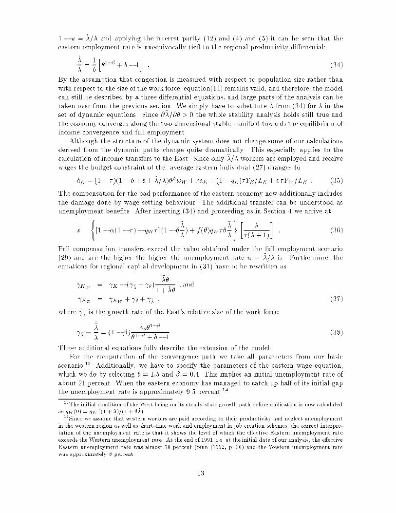
Figure 2 shows the results. Solid lines reproduce the outcome of the basic scenario fromFigure 1 and dashed lines show the corresponding wage setting solution. Compared to Figure1 we have inserted two new panels showing the development of relative income per capitaand the unemployment rate. For that purpose we have skipped the qE-curve which is thesame as in Figure 1 and the r-curve since its shape is also re ected by the C-curve which isstill available.
0 5 10 15 20 25 300.30.40.50.60.70.80.9
0 5 10 15 20 25 30
0.030.060.090.120.15
0 5 10 15 20 25 300
0.03
0.06
0.09
0.12
0 5 10 15 20 25 300.014
0.015
0.016
0.017
θ2 θ
x γ K
E
,γ K
W
γ C u
t t
t t
t t0 5 10 15 20 25 30
0
0.05
0.1
0.15
0.2
0 5 10 15 20 25 30
0.50.60.70.80.9
Figure 2: German Uni�cation: Wage Setting BehaviourSolid Lines: Basic Scenario, Dashed Lines: Wage Setting, Dotted Lines: Wage Setting & Reluctant Fiscal Policy
We have placed the �2 panel in the dominant upper left corner because this curve isessential to understand the remainder of Figure 2. Relative GDP per capita approachesthe steady-state from the much lower initial value of about 0.32 if unemployment exists.Turning towards the regional growth rates, we see that the eastern capital growth rate underunemployment exceeds the corresponding full employment value. This is because the easterneconomy starts from a much more severe initial situation than before. West Germany'scapital growth rate, however, is only insigni�cantly lower in the unemployment scenario. Tounderstand the result it may help to reconsider equation (12). Because of free private capitalmovements � is �xed by regional infrastructure policy. Lower employment in East Germany,LE < �LE , may then have two e�ects: a lower initial share of economy-wide private capitalallocated in eastern Germany and second, a higher capital labour share in each existing�rm in both regions. While the �rst e�ect results in a higher eastern capital growth ratealong the convergence path the second e�ect additionally results in a lower western capitalgrowth rate. Figure 2 shows that mainly the �rst e�ect takes place in our model economy.
14
Hence, worsening investment conditions in East Germany mainly provoke a substitution frominvestment towards consumption rather than a substitution of investment in the East withinvestment in the West. This can also be seen in the gC-panel. The initial growth rate ofconsumption is signi�cantly lower than under perfect market conditions implying a higherinitial level of consumption and a lower initial value of the interest rate.
The employed eastern worker can be identi�ed as the winner of wage setting behaviour.He starts with a higher wage rate as compared to perfect market conditions and experienceshigher wage growth along the adjustment path. The question remains open whether thewestern worker bene�ts from eastern wage setting behaviour. Due to the initially highercapital labour ratio he indeed starts with a higher initial wage as compared to perfect marketconditions. Since the wage rate eventually grows with the steady{state rate, it grows with a(slightly) smaller rate on the convergence path as compared to the perfect market scenario.Hence, eastern wage setting behaviour provides a temporary gain in wages for the westernworker. As the x-panel shows, the western worker pays for his temporary gain in wages witha permanent loss of social transfers that are now received by the unemployed eastern workers.
Transfers required for full compensation for eastern backwardness are now initially morethan 3.5 percentage points higher than under perfect market conditions and lie signi�cantlyabove the compensation rate under perfect market conditions for most of the convergenceprocess. Hence, the model does not support the argument that eastern wage setting behaviourhas been the outcome of deliberate western union policy which takes the burden of additionaltransfers paid by western tax payers into account
If we assume that western tax payers successfully resist full compensation for easternunemployment, the true x-curve would lie somewhere between the solid and the dashed linein Figure 2. This would in turn have the implication that the unemployed eastern populationalso su�ers from wage setting behaviour and that there is only one group that bene�ts fromwage setting which consists of the employed eastern population.
Let us now �nally consider the worst case scenario of our parameterised model. Thiscomprises the assumptions of wage setting behaviour and a reluctant infrastructure spendingpolicy (� = 1:5) and is represented by the dotted lines in Figure 2. It can be seen that bothassumptions together slow down the convergence process considerably. Half of the initialgap in income per capita is now closed 15 years after uni�cation time (instead of 10 years)and after 30 years (instead of 20 years) eastern income per capita has reached 80 percentof the western level. In addition, full compensation for a bad initial position implies thatthe East still receives large amounts of transfers long after uni�cation time. For example,20 years after uni�cation the East still receives more than 7 percent of western tax earnings.Persistent high transfers are necessary because the initially high unemployment rate decreasesonly slowly under the reluctant infrastructure spending scheme. For example, 10 (20) yearsafter uni�cation the eastern unemployment rate is still above 11 (7) percent. In other words,the bill for the East will stay huge into the next decade.
7 Conclusion
The paper has analysed economic growth and regional convergence of uni�ed Germany withina two-region endogenous growth model. The model has emphasised the importance of publicand private capital accumulation in the initially backward region and on the �scal interde-pendence of both regions and its implications on regional convergence of income produced as
15
well as income earned per inhabitant.15 To keep the analysis tractable several other factorswhich certainly also in uence the convergence process have been neglected. Some of thesefactors, like e.g. international capital movements and migration may enhance the speed ofconvergence while other factors, like initially inappropriate human capital the work force mayslow down the adjustment pace.16
The theoretical part of the paper has developed a set of feasible �scal policy rules whichestablish income per capita convergence. A verbal translation of the feasible policy is: When-ever infrastructure per capita in one region is lower as in the other region spend a highershare of tax earnings on infrastructure in this region. If this is not the case spend regionallyidentical shares. Looking back to the huge injection of public cash shows that Germany'sgovernment has followed this rule. The general �scal policy rule, however, neither providesinformation about the speed of convergence nor does it specify the involved costs for citizensof the initially richer region. For that purpose we have calibrated the model with Germandata. Assuming a government that has the objective to compensate the eastern populationfor the relatively bad performance of its economy during the adjustment period, a major�nding was that actual transfers paid by Western tax payers would have been approximatelysu�cient for full compensation, i.e. the equalisation of human wealth in both parts of Ger-many in a perfect market scenario. After introducing wage setting and unemployment in theeastern region we found that actual transfers are no longer su�cient for full compensationfor initial backwardness.
The speed of convergence depends on the future e�ort in infrastructure accumulationin the East.17 We have introduced alternative �scal policy rules which are approximatelyconsistent with the past but generate di�erent patterns of future development. In all casesthe eastern economy converges quite fast. In the most optimistic scenario it will reach 80percent of West Germany's GDP per capita after 20 years. If future governments followa reluctant infrastructure expenditure policy and persistent high unemployment exists, 80percent will be reached about 10 years later.
Why do we think that the results obtained indicate a quite fast adjustment of the Easterneconomy? For a better understanding it may help to compare East Germany's growth per-formance with West Germany's Wirtschaftswunder after World War II. In real internationaldollars West Germany's GDP per capita was 40 percent of the corresponding U.S. level inthe initial period 1950-1955 (data from Summers and Heston, 1995). During this time theprivate investment/GDP ratio reached values between 20 and 25 percent. For the East Ger-man economy that started at a similar initial position we calculate a private investment ratiobetween 38 and 20 percent during the �rst �ve years in our unemployment scenario, a valueapproximately consistent with the actually attained empirical values. In 1990, 40 years afterthe onset of the German Wirtschaftswunder, West Germany had reached 80 percent of theU.S. GDP per capita. In comparison, our analysis suggests that eastern Germany may con-verge much faster and may have caught up 80 percent of its initial gap to West Germany'sGDP per capita after 20 years.
15See e.g. Young (1994) for the importance of factor accumulation for catching-up processes.16In some ways, under direct pressure, the East is setting the West a positive example. Most eastern
companies have now broken out of the straitjacket of nationwide wage bargaining �rst foisted on them by theWest; easterners work long hours and are more exible than western workers; real tape has been slashed.
17The importance of �scal policy in the model does, of course, not imply that there is no need to stream-line the bewildering array of investment promotion schemes since a signi�cant part of the early tax-driveninvestment in the East went, in e�ect, down a black hole.
16
Appendix
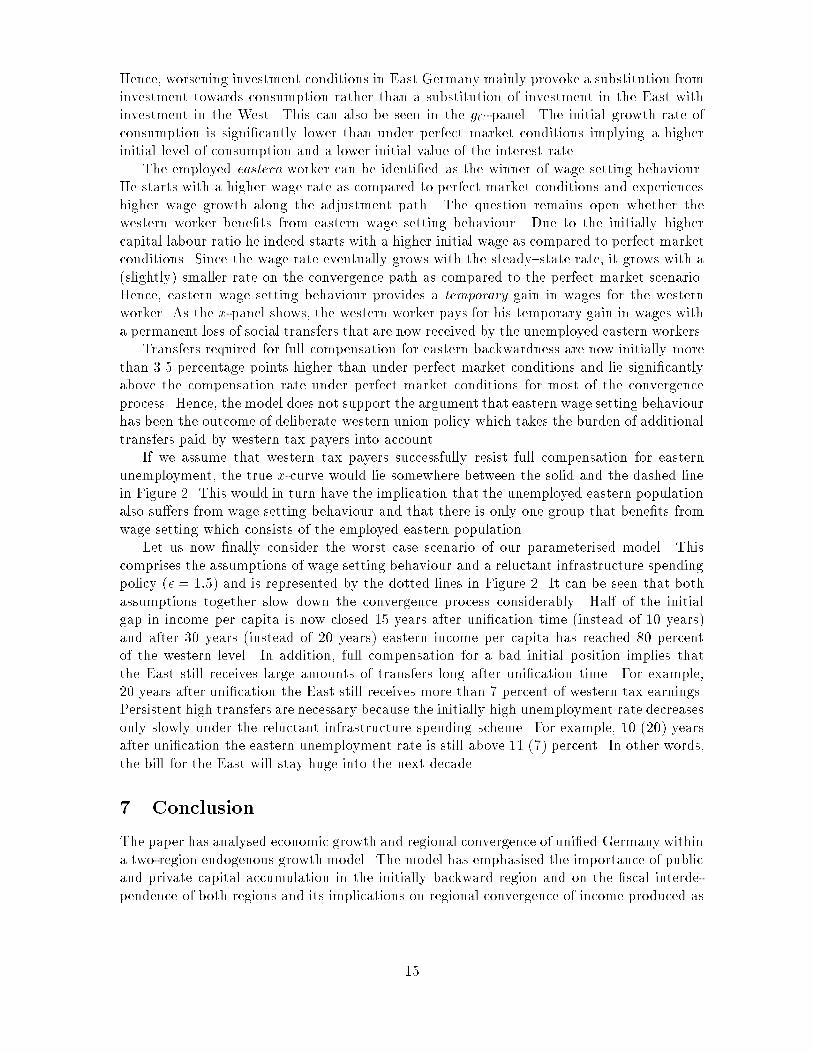
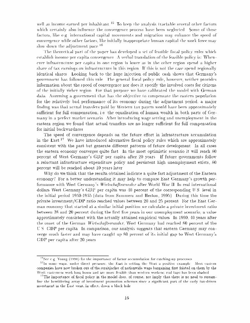
A Brief Introduction to Backward Integration
All solution trajectories converge along the stable manifold towards the steady state (gW?; �?; 1).
A reversion of time, t 7! �t, i.e. a multiplication of the right hand side of the dynamic systemwith (�1) reverses the stability characteristics. Visually this can be thought of as a reversionof the phase diagram. The originally inherently unstable boundary value problem is repre-sented as a stable initial value problem which can be solved by standard methods. We use afourth order Runge-Kutta-Fehlberg algorithm with stopping criterion � � �(0).
0.10.15
0.2
0.60.8
11.2
1.4
0.21
0.22
0.23
0.24
0.25
0.26
gW
θ
χ
The Stable Manifold: Basic Scenario
As starting values for backward integration, we iteratively use the values of a cycle in thegW {�-plane around the steady-state:for i=0 to 2 step 0.00001; gW = gW
? + � sin(i�); � = �? + � cos(i�); � = �? � �,
where the parameter � speci�es the initial deviation from the steady- state, which is setto 10�12. Since the cycle intersects every solution trajectory exactely once this proceduregenerates a set of possible solution trajectories on the stable manifold as shown in the Figure. From the subset of solution trajectories that end at the 'right' side of �, i.e. at �(0) = 0:4we select the one that matches most closely gW (0) = gW
?(1 + �)=(1 + �(0)�). Once thetrajectory is obtained time is reversed again so that the sequence of solution values providesthe forward looking time path for the original system. This system starts � = 0:4 and in asituation where the western region was close to its steady-steady before uni�cation. Forwardlooking the system then converges towards the steady-state, stopping at a distance of 10�12
from the steady-state.
17
References
Barro, R.J., 1990, Government Spending in a Simple Model of Endogenous Growth, Journalof Political Economy 98, 103{ S.125.
Barro, R.J, 1991, Eastern Germany's Long Haul, Wall Street Journal, 3 May 1991, p. A10.
Barro, R.J. and X. Sala-i-Martin, 1991, Convergence across States and Regions, BrookingsPapers on Economic Activity 1, 107{ 182.
Burda, M. and M. Funke, 1993, German Trade Unions after Uni�cation - Third Degree WageDiscriminating Monopolists?, Weltwirtschaftliches Archiv 129, 537{560.
Burda, M. and M. Funke, 1995, Eastern Germany: Can't We Be More Optimistic?, Ifo Stu-dien 41, 327{354.
Brunner, M. and H. Strulik, 1998, Solution of Perfect Foresight Saddlepoint Problems: ASimple Method and Applications, Working Paper, Hamburg University.
Caselli, F. and Ventura, J., 1999, A Representative Consumer Theory of Distribution, Uni-versity of Chicago Working Paper.
Deutsche Bundesbank, 1996, The Debate on Public Transfers in the Wake of German Reuni-�cation , Monthly Report of the Deutsche Bundesbank 48, No. 10, 17{30.
Deutsches Institut fuer Wirtschaftsforschung (DIW), 1994, Wochenbericht 27/94, Berlin.
Deutsches Institut fuer Wirtschaftsforschung (DIW), 1995, Wochenbericht 31/95, Berlin.
Dornbusch, R, and H. Wolf, 1992, Economic Transition in Eastern Germany, Brookings Pa-pers on Economic Activity 1, 235{272.
Duggal, V.G., C. Saltzman, and L. R. Klein, 1999, Infrastructure and Productivity: A Non-linear Approach, Journal of Ecoonometrics 92, 47{74.
Englmann, F.C. and U. Walz, 1995, Industrial Centers and Regional Growth in the Presenceof Local Inputs and Knowledge Spillovers, Journal of Regional Science 35, 3{27.
Hughes Hallet, A. and Y. Ma, 1993, East Germany, West Germany, and their MezzogiornoProblem: A Parable for European Economic Integration, Economic Journal 103, 416{428.
Kocherlakota, N.R. and K.-M. Yi, 1997, Is there Endogenous Long-Run Growth? Evidencefrom the United States and the United Kingdom, Journal of Money, Credit, and Banking 29,235{262.
Ono, Y. and A. Shibata, 1992, Spill-over E�ects of Supply- Side Changes in a Two-CountryEconomy with Capital Accumulation, Journal of International Economics 33, 127{146
Sinn, G. and H.-W. Sinn, 1992, Jumpstart: The Economic Uni�cation of Germany, Cam-bridge, MA (MIT-Press). Statistisches Bundesamt (1997), Statistisches Jahrbuch fuer dieBundesrepublik Deutschland, Wiesbaden.
Sturm, J.-E., G.H. Kuper and J. de Haan, 1998, Modelling Government Investment andEconomic Growth on a Macro Level: A Review, in: Brakman, S., H. van Ees, and S.K.
18

Kuipers, eds., Market Behaviour and Macroeconomic Modelling, London (MacMillan/St.Martins Press).
Summers, R. and A. Heston, 1995, Penn World Table (Mark 5.6a), available on diskette fromthe National Bureau of Economic Research, Cambridge MA.
Young, Alwyn, 1994, Lessons from the East Asian NICS: A contrarian view, European Eco-nomic Review 38, 964{973.
19


