23
Copyleft Copyleft 2005 by Media Lab 2005 by Media Lab 1 Ordinary Differential Equations Ordinary Differential Equations Boundary Value Problems Boundary Value Problems
| Date post: | 02-Jan-2016 |
| Category: |
Documents |
| Upload: | arthur-barnett |
| View: | 220 times |
| Download: | 0 times |

Copyleft Copyleft 2005 by Media Lab 2005 by Media Lab 11
Ordinary Differential EquationsOrdinary Differential EquationsBoundary Value ProblemsBoundary Value Problems

Copyleft Copyleft 2005 by Media Lab 2005 by Media Lab 22
14.1 Shooting Method for Solving Linear BVPs14.1 Shooting Method for Solving Linear BVPs
• We investigate the second-order, two-point boundary-value problem of the form
with Dirichlet boundary conditions
Or Neuman boundary conditions
Or mixed boundary condition
),,( yyxfy bxa ,
,)( ay )(by
,)( ay )(by
,)()( 1 aycay )()( 2 bycby
Copyleft Copyleft 2005 by Media Lab 2005 by Media Lab 33
14.1 Shooting Method for Solving Linear BVPs14.1 Shooting Method for Solving Linear BVPs
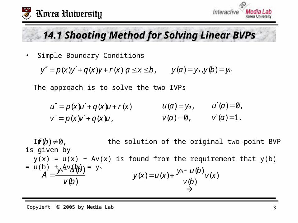
• Simple Boundary Conditions
The approach is to solve the two IVPs
If the solution of the original two-point BVP is given by y(x) = u(x) + Av(x) is found from the requirement that y(b) = u(b) + Av(b) = yb
,),()()( bxaxryxqyxpy
,)()(
),()()(
uxqvxpv
xruxquxpu
,0)(
,)(
av
yau a
.1)(
,0)(
av
au
).()(
)()()( xv
bv
buyxuxy
b
,0)( bv
ba ybyyay )(,)(
)(
)(
bv
buyA
b

Copyleft Copyleft 2005 by Media Lab 2005 by Media Lab 44
14.3 Shooting Method for Solving Linear BVPs14.3 Shooting Method for Solving Linear BVPs
• EX14.1
• convert to the pair of initial-value problems
,2y
xy
,10)1( y ,0)2( y
vx
v
ux
u
2
,2
,0)1(
,10)1(
v
u
,0)1(
,0)1(
v
u
,21 ww ,2
2wx
xw
,43 ww ,2
44 wx
w
).()(
)(0)( 3
3
11 xw
bw
bwxwxy

Copyleft Copyleft 2005 by Media Lab 2005 by Media Lab 55
14.1 Shooting Method for Solving Linear BVPs14.1 Shooting Method for Solving Linear BVPs
• General Boundary Condition at x = b
The condition at x=b involves a linear combination of y(b) and y’(b)
The approach is to solve the two IVPs
If there is a unique solution, given by
)()()( xryxqyxpy
,)()(
),()()(
uxqvxpv
xruxquxpu
,0)(
,)(
av
yau a
.1)(
,0)(
av
au
).()()(
)()()()( xv
bcvbv
bcubuyxuxy
b
0)()( bcvbv
ba ybcybyyay )()(,)(

Copyleft Copyleft 2005 by Media Lab 2005 by Media Lab 66
14.3 Shooting Method for Solving Linear BVPs14.3 Shooting Method for Solving Linear BVPs
• General Boundary Condition at Both Ends of the Interval
the approach is to solve two IVPs
If , there is a unique solution, given by
)()()( xryxqyxpy
,)()( 1 ayaycay .)()( 2 bybycby
,)()(
),()()(
uxqvxpv
xruxquxpu
,1)(
,0)(
av
au
.)(
,)(
1cav
yau a
).()()(
)()()()(
2
2
xvbvcbv
bucbuyxuxy
b
0)()( 2 bvcbv
Copyleft Copyleft 2005 by Media Lab 2005 by Media Lab 77
14.3 Shooting Method for Solving Linear BVPs14.3 Shooting Method for Solving Linear BVPs
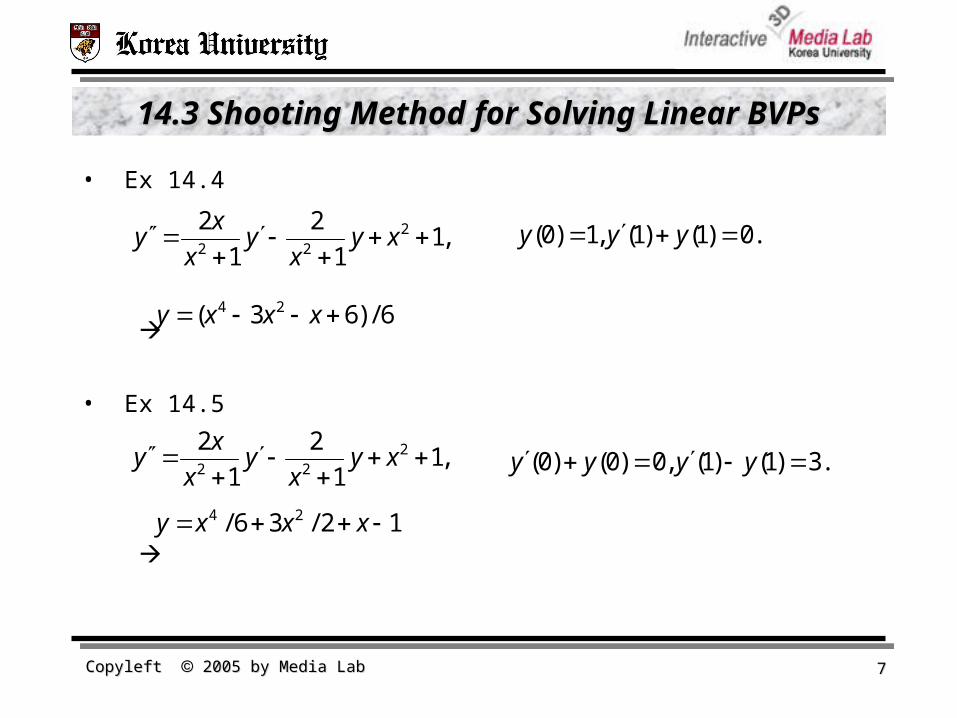
• Ex 14.4
• Ex 14.5
,11
2
1
2 222
xyx
yx
xy .0)1()1(,1)0( yyy
6/)63( 24 xxxy
,11
2
1
2 222
xyx
yx
xy .3)1()1(,0)0()0( yyyy
12/36/ 24 xxxy
Copyleft Copyleft 2005 by Media Lab 2005 by Media Lab 88
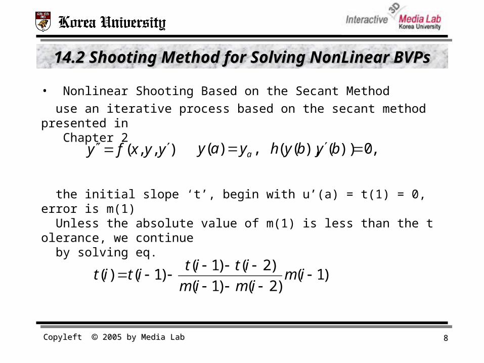
14.2 Shooting Method for Solving NonLinear BVPs14.2 Shooting Method for Solving NonLinear BVPs
• Nonlinear Shooting Based on the Secant Method
use an iterative process based on the secant method presented in Chapter 2
the initial slope ‘t’, begin with u’(a) = t(1) = 0, error is m(1) Unless the absolute value of m(1) is less than the tolerance, we continue by solving eq.
),,,( yyxfy ,)( ayay ,0))(),(( bybyh
).1()2()1(
)2()1()1()(
imimim
itititit

Copyleft Copyleft 2005 by Media Lab 2005 by Media Lab 99
14.2 Shooting Method for Solving NonLinear BVPs14.2 Shooting Method for Solving NonLinear BVPs
• EX 14.6
y = 1/(x+1)
,2 yyy ,1)0( y .025.0)1()1( yy

Copyleft Copyleft 2005 by Media Lab 2005 by Media Lab 1010
14.2 Shooting Method for Solving NonLinear BVPs14.2 Shooting Method for Solving NonLinear BVPs
• Nonlinear Shooting Using Newton’s Method
begin by solving the initial-value problem
Check for convergence:
if |m| < tol, stop;
Otherwise, update t:
),,,( yyxfy ,)( ayay .)( byby
),,,(),,(''
),,,(
uuxfvuuxvfv
uuxfu
uu
,0)(
,)(
av
yau a
.1)(
,)(
av
tau k
;),( bk ytbum
);,(/1 kkk tbvmtt

Copyleft Copyleft 2005 by Media Lab 2005 by Media Lab 1111
14.2 Shooting Method for Solving NonLinear BVPs14.2 Shooting Method for Solving NonLinear BVPs
• EX 14.8
,][ 2
y
yy
,2)1( y,1)0( y
,][ 12 uuu ,1)0( u .)0( ktu
.][2),,(
,)1(][),,(
1
22
uuuuxf
uuuuxf
u
u
,][2][ 122
uuvuuvv ,0)0( v .1)0( v

Copyleft Copyleft 2005 by Media Lab 2005 by Media Lab 1212
14.3 Finite Difference Method for Solving Linear BVPs14.3 Finite Difference Method for Solving Linear BVPs
• Replace the derivatives in the differential equation by finite-difference approximations (discussed in Chapter 11).
• We now consider the general linear two-point boundary-value problem
• with boundary conditions
• To solve this problem using finite-differences, we divide the interval [a, b] into n subintervals, so that h=(b-a)/n. To approximate the function y(x) at the points we use the central difference formulas from Chapter 11:
,),()()( bxaxryxqyxpy
,)(,)( byay
,)1(, 11 hnaxhax n
h
yyxy
h
yyyxy ii
iiii
i 2)(,
2)( 11
211

Copyleft Copyleft 2005 by Media Lab 2005 by Media Lab 1313
Finite Difference Method for Solving Linear BVPsFinite Difference Method for Solving Linear BVPs
• Substituting these expressions into the BVP and writing as ____ as and as gives
• Further algebraic simplification leads to a tridiagonal system for the unknowns viz.
• where and .
)( ixp)(, ii xqp ,iq )( ixr ir
iiiii
iiii ryq
h
yyp
h
yyy
2
2 112
11
,,, 11 nyy
,1,,1,2
1)2(2
1 21
21
nirhy
hpyqhy
hp iiiiiii
)(0 ayy )(byyn
Copyleft Copyleft 2005 by Media Lab 2005 by Media Lab 1414
Finite Difference Method for Solving Linear BVPsFinite Difference Method for Solving Linear BVPs
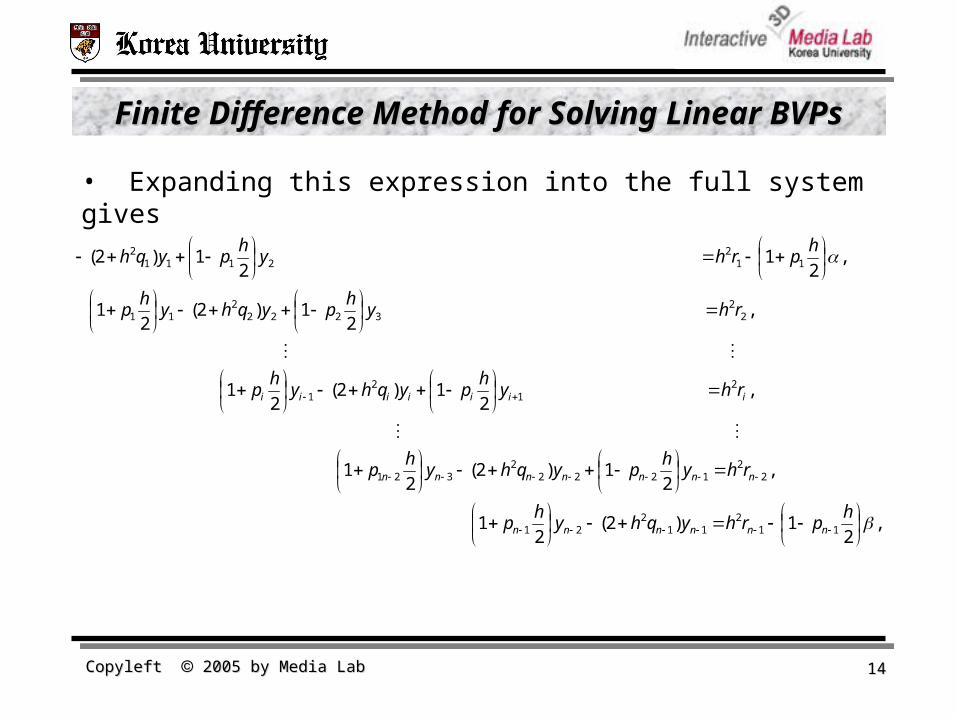
• Expanding this expression into the full system gives
,2
1)2( 2
1
,2
1)2(2
1
, 2
1)2(2
1
, 2
1)2(2
1
,2
1 2
1)2(
112
112
21
22
12222
321
21
21
22
32222
11
112
21112
hprhyqhy
hp
rhyh
pyqhyh
p
rhyh
pyqhyh
p
rhyh
pyqhyh
p
hprhy
hpyqh
nnnnnn
nnnnnnn
iiiiiii

Copyleft Copyleft 2005 by Media Lab 2005 by Media Lab 1515
Example 14.9 A Finite-Difference ProblemExample 14.9 A Finite-Difference Problem
• Use the finite-difference method to solve the problem
• with y(0)=y(4)=0 and n=4 subintervals.• Using the central difference formula for the second derivative, we find that the differential equation becomes the system.
• For this example, h = 1 ,i =1, y = 0, and i = 3, y = 0. Substituting this values, we obtain
4,x0 ),4( xxyy
1,2,3.i ),4(2
)(2
11
iii
iiii xxy
h
yyyxy
).43(320
),42(22
),41(102
323
2123
112
yyy
yyyy
yyy
Copyleft Copyleft 2005 by Media Lab 2005 by Media Lab 1616
Example 14.9 A Finite-Difference ProblemExample 14.9 A Finite-Difference Problem
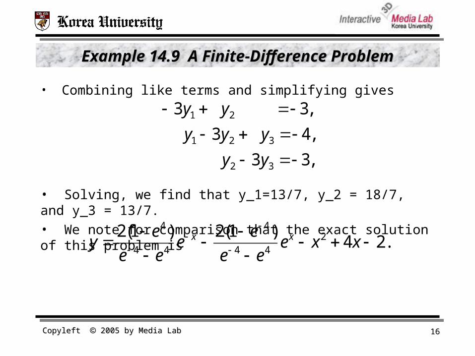
• Combining like terms and simplifying gives
• Solving, we find that y_1=13/7, y_2 = 18/7, and y_3 = 13/7.• We note for comparison that the exact solution of this problem is
,33
,4 3
,3 3
32
321
21
yy
yyy
yy
.24)1(2)1(2 2
44
4
44
4
xxeee
ee
ee
ey xx

Copyleft Copyleft 2005 by Media Lab 2005 by Media Lab 1717
Example 14.9 A Finite-Difference ProblemExample 14.9 A Finite-Difference Problem
Copyleft Copyleft 2005 by Media Lab 2005 by Media Lab 1818
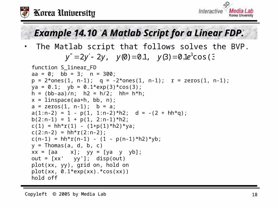
Example 14.10 A Matlab Script for a Linear FDP.Example 14.10 A Matlab Script for a Linear FDP.• The Matlab script that follows solves the BVP.
cos(3).1.0)3( ,1.0)0( ,22 3eyyyyy function S_linear_FDaa = 0; bb = 3; n = 300;p = 2*ones(1, n-1); q = -2*ones(1, n-1); r = zeros(1, n-1);ya = 0.1; yb = 0.1*exp(3)*cos(3);h = (bb-aa)/n; h2 = h/2; hh= h*h;x = linspace(aa+h, bb, n);a = zeros(1, n-1); b = a;a(1:n-2) = 1 - p(1, 1:n-2)*h2; d = -(2 + hh*q);b(2:n-1) = 1 + p(1, 2:n-1)*h2; c(1) = hh*r(1) - (1+p(1)*h2)*ya;c(2:n-2) = hh*r(2:n-2);c(n-1) = hh*r(n-1) - (1 - p(n-1)*h2)*yb;y = Thomas(a, d, b, c)xx = [aa x]; yy = [ya y yb];out = [xx' yy']; disp(out)plot(xx, yy), grid on, hold onplot(xx, 0.1*exp(xx).*cos(xx))hold off

Copyleft Copyleft 2005 by Media Lab 2005 by Media Lab 1919
Example 14.10 A Matlab Script for a Linear FDP.Example 14.10 A Matlab Script for a Linear FDP.

Copyleft Copyleft 2005 by Media Lab 2005 by Media Lab 2020
14.4 FDM for Solving Nonlinear BVPs14.4 FDM for Solving Nonlinear BVPs
• We consider the nonlinear ODE-BVP of the form
• Assume that there are constants and such that
• Use a finite-difference grid with spacing and let denote the result of evaluating at using for . • The ODE then becomes the system
• An explicit iteration scheme, analogous to the SOR method
• where and The process will converge for
cos(3).1.0)3( ,1.0)0( ,22 3eyyyyy *
* Q,Q *P*
** |),,(| ),,(0 PyyxfandQyyxfQ yy
,/2 *Ph iff ix )2/()( 11 hyy ii iy
.02
211
i
iii fh
yyy
,2)1(2
1 211 iiiii fhyyyy
0y .ny .2/*2Qhw

Copyleft Copyleft 2005 by Media Lab 2005 by Media Lab 2121
Example 14.12 Solving a Nonlinear BVP by Using FDMExample 14.12 Solving a Nonlinear BVP by Using FDM
• Consider again the nonlinear BVP
• We illustrate the use of the iterative procedure just outlined by taking a grid with h = ¼. The general form of the difference equation is
• where
.2)1( ,1)0( ,
2
yyy
yy
,2)1(2
1 211 iiiii fhyyyy
.
)1(4
2)2/()(2
2111
21
211
i
iiii
i
iii yh
yyyy
y
hyyf

Copyleft Copyleft 2005 by Media Lab 2005 by Media Lab 2222
Example 14.12 Solving a Nonlinear BVP by Using FDMExample 14.12 Solving a Nonlinear BVP by Using FDM
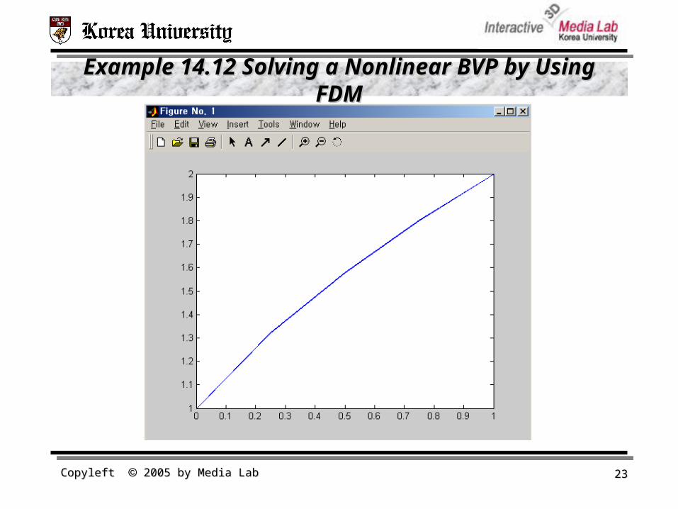
• Substituting the rightmost expression for f_i into the equation for y_i, we obtain
• The computed solution after 10 iterations agrees very closely with the exact solution.
.4
22
)1(2
1 2111
21
11
i
iiiiiiii y
yyyyyyyy
function S_nonlinear_FDya = 1; yb = 2; a = 0; b = 1;max_it = 10; n = 4; w = 0.1; ww = 1/(2*(1+w)); h = (b-a)/ny(1:n-1) = 1for k = 1:max_it y(1) = ww*(ya+2*w*y(1)+y(2)+(ya^2-2*ya*y(2)+y(2)^2)/(4*y(1))); y(2) = ww*(y(1)+2*w*y(2)+y(3)+(y(1)^2-2*y(1)*y(3)+y(3)^2)/(4*y(2))); y(3) = ww*(y(2)+2*w*y(3)+yb+(y(2)^2-2*y(2)*yb+yb^2)/(4*y(3)));endx = [ a a+h a+2*h a+3*h b ]; z = [ ya y yb ];plot(x, z), hold on, zz = sqrt(3*x+1); plot(x, zz), hold off
Copyleft Copyleft 2005 by Media Lab 2005 by Media Lab 2323
Example 14.12 Solving a Nonlinear BVP by Using FDMExample 14.12 Solving a Nonlinear BVP by Using FDM


