33
Copyright © 2009 Pearson Addison-Wesley. All rights reserved. Chapter 3 Spending, Income, and Interest Rates
| Date post: | 22-Dec-2015 |
| Category: |
Documents |
| View: | 215 times |
| Download: | 0 times |

Copyright © 2009 Pearson Addison-Wesley. All rights reserved.
Chapter 3
Spending, Income, and Interest Rates

Copyright © 2009 Pearson Addison-Wesley. All rights reserved. 3-2
Theory of Business Cycles: Outline
• Ch 3: Spending, Income, and Interest Rates– Use the Keynesian Cross Model to derive the IS curve
• Ch 4: Monetary and Fiscal Policy in the IS/LM Model– Use equilibrium in the money market to derive the LM curve
– Combine the IS and LM curves to determine Y and i
• Ch 5: The Government Budget, Foreign Borrowing,
and the Twin Deficits
• Ch 6: International Trade, Exchange Rates, and Macroeconomic Policy

Copyright © 2009 Pearson Addison-Wesley. All rights reserved. 3-3
The “Great Moderation”
• The goal of monetary and fiscal policy is to dampen business cycle fluctuations and to promote steady economic growth.
• Since 1985, business cycle fluctuations have noticeably diminished.
• This data has caused debate among economists:– Have there been fewer shocks since 1985?
– Or were monetary and fiscal policy more effective in offsetting shocks?

Copyright © 2009 Pearson Addison-Wesley. All rights reserved. 3-4
Figure 3-1 Real GDP Growth in the United States, 1950–2007

Copyright © 2009 Pearson Addison-Wesley. All rights reserved. 3-5
Aggregate Demand and Supply
• Aggregate Demand (AD) is the total amount of desired spending expressed in current (or nominal) dollars.– A demand shock is a significant change in desired spending by
consumers, business firms, the government, or foreigners.• Algebraically, any change in C, I, G or NX
• Aggregate Supply (AS) is the amount that firms are will to produce at any given price level.– A supply shock is a significant change in costs of production for
business firms, including wages and the prices of raw materials, like oil.
• AS and supply shocks will be considered in Chapters 7 and 8.

Copyright © 2009 Pearson Addison-Wesley. All rights reserved. 3-6
Modeling Preliminaries
• Simplifying assumption:– The price level (P) is fixed in the short run.
• Implication: All changes in AD automatically cause changes in real GDP by the same amount and in the same direction.
• The variables that an economic theory tries to explain are called endogenous variables.– Examples: Output and interest rates
• Exogenous variable are those that are relevant but whose behavior the theory does not attempt to explain; their values are taken as given.– Examples: Money supply, government spending, tax rates

Copyright © 2009 Pearson Addison-Wesley. All rights reserved. 3-7
Consumption and Savings
• The consumption function is any relationship that describes the determinants of consumption spending.
• General linear form: C = Cα + c(Y – T) where…– Cα = Autonomous consumption– c = marginal propensity to consume– c(Y – T) = induced consumption
• Savings (S) = Y – T – C Substituting in C from above yields:
S = Y – T – [Cα + c(Y – T)]
S = – Cα + (1 – c)(Y – T)] where…– (1 – c) = marginal propensity to save (s)

Copyright © 2009 Pearson Addison-Wesley. All rights reserved. 3-8
Figure 3-2 A Simple Hypothesis Regarding Consumption Behavior

Copyright © 2009 Pearson Addison-Wesley. All rights reserved. 3-9
Figure 3-3 Consumption, Saving, and Disposable Income, 1929–2007

Copyright © 2009 Pearson Addison-Wesley. All rights reserved. 3-10
Factors Affecting Cα
• Interest Rates (r): When r↓ borrowing is cheaper for consumers Cα↑ – Example: Low interest rates in 2001-04 stimulated consumption of
automobiles and other consumer products.
• Household Wealth (W) is the total net value of all household assets (minus any debt), including the market value of homes, possessions such as automobiles, and financial assets such as stocks, bonds, and bank accounts.– If W↑ household spending can rise even if income is fixed
Cα↑ – Example: The 1990s stock market boom raised consumption.
Copyright © 2009 Pearson Addison-Wesley. All rights reserved. 3-11
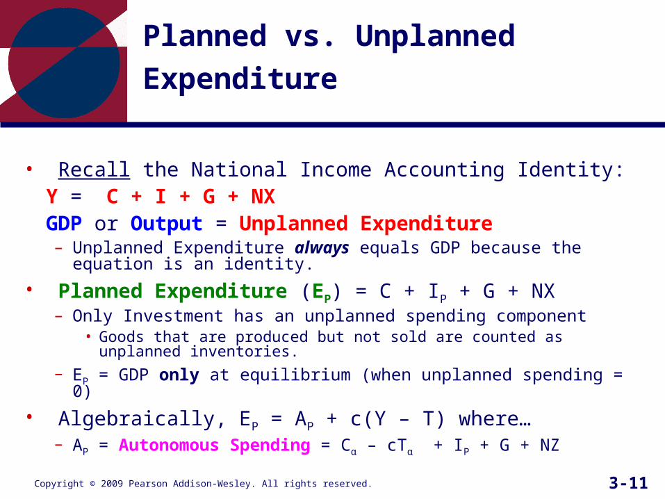
Planned vs. Unplanned Expenditure
• Recall the National Income Accounting Identity:Y = C + I + G + NX GDP or Output = Unplanned Expenditure
– Unplanned Expenditure always equals GDP because the equation is an identity.
• Planned Expenditure (EP) = C + IP + G + NX– Only Investment has an unplanned spending component
• Goods that are produced but not sold are counted as unplanned inventories.
– EP = GDP only at equilibrium (when unplanned spending = 0)
• Algebraically, EP = AP + c(Y – T) where…– AP = Autonomous Spending = Cα – cTα + IP + G + NZ

Copyright © 2009 Pearson Addison-Wesley. All rights reserved. 3-12
The Equilibrium of the Economy
• At equilibrium, Y = EP
Y = AP + cY (assuming T = 0)
To find equilibrium Y, solve the above equation for Y:
(1 – c)Y = AP
sY = Ap
Y = (1/s) AP
• If the level of AP changes over time by ∆AP , then thechange in output, ∆Y, is given by:
∆Y = (1/s) ∆AP
• 1/s is called the multiplier because it shows how each additional dollar of autonomous spending results in a greater than $1 increase in equilibrium output.

Copyright © 2009 Pearson Addison-Wesley. All rights reserved. 3-13
Table 3-1 Comparison of the Economy’s “Always True” and Equilibrium Situations

Copyright © 2009 Pearson Addison-Wesley. All rights reserved. 3-14
Figure 3-4 How Equilibrium Income Is Determined

Copyright © 2009 Pearson Addison-Wesley. All rights reserved. 3-15
Figure 3-5 The Change in Equilibrium Income Caused by a $500 Billion Increase in Autonomous Planned Spending

Copyright © 2009 Pearson Addison-Wesley. All rights reserved. 3-16
Shifts in Planned Spending
• Recall: EP = C + IP + G + NX = AP + cY
where AP = Cα – cTα + IP + G + NZ
• Any increase in AP will shift up EP on the Keynesian Cross Diagram.– Effect on Y: ∆Y = (1/s) ∆AP
• If c changes, the EP line will rotate
• If the effect on Y is negative, fiscal policy can be used to offset the effect.

Copyright © 2009 Pearson Addison-Wesley. All rights reserved. 3-17
Figure 3-6 Relation of the Various Components of Autonomous Planned Spending to the Interest Rate

Copyright © 2009 Pearson Addison-Wesley. All rights reserved. 3-18
Figure 3-7 Relation of the IS Curve to the Demand for Autonomous Spending
Copyright © 2009 Pearson Addison-Wesley. All rights reserved. 3-19
Chapter Equations

Copyright © 2009 Pearson Addison-Wesley. All rights reserved. 3-20
Chapter Equations
Changes in Aggregate DemandChanges in Real GDP (3.1)
Fixed Price Level
(3.2)E C I G NX
General Linear Form
( ) (3.3)aC C c Y T

Copyright © 2009 Pearson Addison-Wesley. All rights reserved. 3-21
Chapter Equations
General Linear Form
( )
(1 )( )
Numerical Example
500 0.75( )
500 0.25( ) (3.4)
a
a
S Y T C Y T C c Y T
C c Y T
S Y T C Y t Y T
Y T
Copyright © 2009 Pearson Addison-Wesley. All rights reserved. 3-22
Chapter Equations
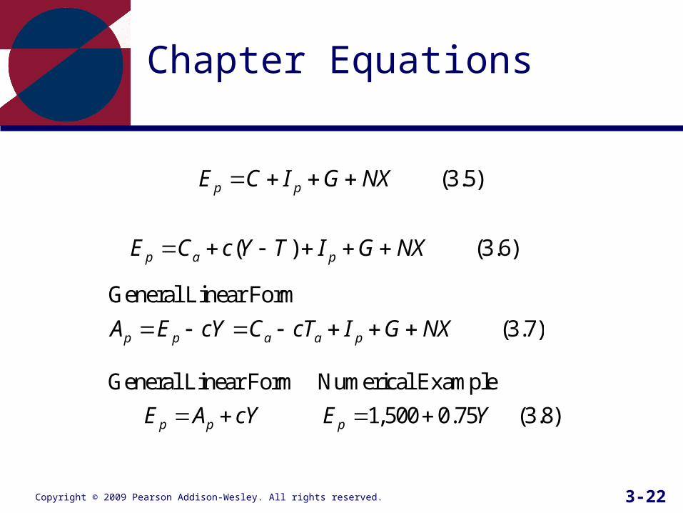
(3.5)p pE C I G NX
( ) (3.6)p a pE C c Y T I G NX
General Linear Form
(3.7)p p a a pA E cY C cT I G NX
General Linear Form Numerical Example
1,500 0.75 (3.8)p p pE A cY E Y
Copyright © 2009 Pearson Addison-Wesley. All rights reserved. 3-23
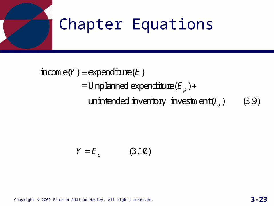
Chapter Equations
income( ) expenditure( )
Unplanned expenditure( )
unintended inventory investment( ) (3.9)
p
u
Y E
E
I
(3.10)pY E

Copyright © 2009 Pearson Addison-Wesley. All rights reserved. 3-24
Chapter Equations
(1 ) (3.11)pc Y A
General Linear Form Numerical Example
0.25 1,500 (3.12)psY A Y
General Linear Form Numerical Example
1,5006,000 (3.13)
0.25pAY Ys
Copyright © 2009 Pearson Addison-Wesley. All rights reserved. 3-25
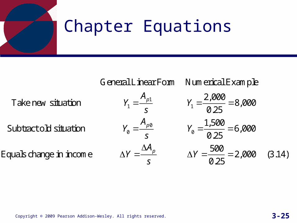
Chapter Equations
11 1
00 0
General Linear Form Numerical Example
2,000Take new situation 8,000
0.25
1,500Subtract old situation 6,000
0.25
500Equals change in income 2,000 (3.14)
0.25
p
p
p
AY Y
sA
Y YsA
Y Ys

Copyright © 2009 Pearson Addison-Wesley. All rights reserved. 3-26
Chapter Equations
General Linear Form Numerical Example
1 1multiplier ( ) 4.0 (3.15)
0.25p p
Y Yk
A s A
(3.16)p a a pA C c T I G NX

Copyright © 2009 Pearson Addison-Wesley. All rights reserved. 3-27
Chapter Equations
(3.17)T G I NX S
1 1Balanced budget multiplier 1.0 (3.18)
c c
s s s

Copyright © 2009 Pearson Addison-Wesley. All rights reserved. 3-28
Appendix Equations
(1)
(2)

Copyright © 2009 Pearson Addison-Wesley. All rights reserved. 3-29
Appendix Equations
(3)
(4)
(5)

Copyright © 2009 Pearson Addison-Wesley. All rights reserved. 3-30
Appendix Equations
(6)

Copyright © 2009 Pearson Addison-Wesley. All rights reserved. 3-31
Appendix Equations
(7)
(8)

Copyright © 2009 Pearson Addison-Wesley. All rights reserved. 3-32
Appendix Equations
(9)
(10)
(11)

Copyright © 2009 Pearson Addison-Wesley. All rights reserved. 3-33
Appendix Equations
(12)


