Page 1
Radar Horizon Estimation from Monoscopic Shadow Photogrammetry of Radar Structures:
A Case Study in the South China Sea
by
James E. Luttrull
A Thesis Presented to the
Faculty of the USC Graduate School
University of Southern California
In Partial Fulfillment of the
Requirements for the Degree
Master of Science
Geographic Information Science and Technology
May 2018
Page 2
Copyright © 2018 by James E. Luttrull
Page 3
iii
Quaesita Marte Tuenda Arte
Page 4
iv
Table of Contents
List of Figures ............................................................................................................................... vii
List of Tables ................................................................................................................................. ix
Acknowledgements ..........................................................................................................................x
Abbreviations and Terminology .................................................................................................... xi
Abstract ......................................................................................................................................... xii
Chapter 1 Introduction .................................................................................................................... 1
1.1. Motivation ...........................................................................................................................1
1.2. Research Objective .............................................................................................................2
1.3. Scope & Data ......................................................................................................................3
1.3.1. Data ............................................................................................................................6
Chapter 2 Background and Literature Review................................................................................ 7
2.1. The South China Sea in History and International Relations .............................................7
2.1.1. Access to Trade & Resources ....................................................................................8
2.1.2. SCS as Path of Invasion .............................................................................................9
2.2. South China Sea Border Claims........................................................................................10
2.2.1. China’s Claim ..........................................................................................................10
2.2.2. Other Claimants .......................................................................................................12
2.3. Anti-Access & Area Denial ..............................................................................................14
2.4. Radio Propagation and Radar Line of Sight .....................................................................17
2.4.1. Radar Height as Measure of Range..........................................................................17
2.4.2. Radar Beyond Line of Sight.....................................................................................19
2.5. Monoscopic Photogrammetry for Shadow Analysis ........................................................20
2.6. GIS Studies of Military Radar ..........................................................................................22
Page 5
v
Chapter 3 Methodology ................................................................................................................ 25
3.1. Data ...................................................................................................................................26
3.1.1. Imagery ....................................................................................................................26
3.1.2. Weapon System Data ...............................................................................................28
3.1.3. Geospatial Data ........................................................................................................28
3.2. Procedure ..........................................................................................................................30
3.2.1. Data Preparation and Preprocessing ........................................................................30
3.2.2. Imagery Analysis .....................................................................................................33
3.2.3. Buffer Creation ........................................................................................................40
3.2.4. Combined Analysis ..................................................................................................43
Chapter 4 Results .......................................................................................................................... 45
4.1. Coverage Results...............................................................................................................45
4.1.1. General Assessment of Coverage ............................................................................48
4.1.2. Gap Estimation.........................................................................................................49
4.1.3. Horizons at Fixed Distance ......................................................................................49
4.2. Radar & Weapon System Cooperation & Range Comparison .........................................49
4.2.1. Assessment of Overlap.............................................................................................54
4.3. Range Corrections and Calculations .................................................................................56
4.3.1. CSIS/AMTI Assumed Tower Height.......................................................................56
4.3.2. Adjusting for CSIS/AMTI Range Estimation ..........................................................57
4.3.3. Utilizing CSIS/AMTI Assumed Tower Heights ......................................................57
4.3.4. Final Coverage Differences .....................................................................................59
Chapter 5 Conclusions .................................................................................................................. 64
5.1. Assessment of Methodology & Results ............................................................................64
Page 6
vi
5.2. Study Assumptions ...........................................................................................................66
5.3. Study Limitations and Sources of Inaccuracy...................................................................66
5.4. Conclusions & Future Work .............................................................................................67
References ..................................................................................................................................... 70
Appendix A: Data Notes ............................................................................................................... 77
Appendix B: Labelled Imagery of Identified Radar Zones........................................................... 78
Appendix C: Weapon System Ranges .......................................................................................... 85
Appendix D: Equations & Syntaxes ............................................................................................. 89
Page 7
vii
List of Figures
Figure 1: GIS and RS Publishings of Ranges and Radar Tower Identification. ............................. 3
Figure 2: Mischief Reef, July 2016................................................................................................. 4
Figure 3: Fiery Cross Reef, June 2016............................................................................................ 5
Figure 4: Subi Reef, July 2016........................................................................................................ 5
Figure 5: Competing Claims for the SCS. .................................................................................... 10
Figure 6: Original 1940s "U-Shaped Line" with 11 Dashes ......................................................... 11
Figure 7: Competing Claims and Natural Resources .................................................................... 14
Figure 8: Visual Depiction of Horizon Trigonometry. ................................................................. 18
Figure 9: 1:1,250 and 1:23,000 Scale of Radar Array. ................................................................. 27
Figure 10: CSIS Identification of Island Features, with Inlay of Radar Array. ............................ 27
Figure 11: Fiery Cross Reef, Manual Centroid Creation. ............................................................. 29
Figure 12: Project Methodology ................................................................................................... 31
Figure 13: Data Preprocessing and Integration Model ................................................................. 32
Figure 14: Zone FC2 ..................................................................................................................... 32
Figure 15: Fiery Cross Reef Radar Zones..................................................................................... 35
Figure 16: Mischief Reef Radar Zones ......................................................................................... 36
Figure 17: Subi Reef Radar Zones ................................................................................................ 37
Figure 18: Imagery Analysis Model ............................................................................................. 38
Figure 19: Example Shadow Measurement in Multispectral Imagery ......................................... 39
Figure 20: Buffer Creation Model ................................................................................................ 41
Figure 21: Buffer Selections ......................................................................................................... 43
Figure 22: Combined Analysis Model .......................................................................................... 44
Page 8
viii
Figure 23: Final Radar Horizon Calculations from Shadow Analysis Method ............................ 46
Figure 24: Radar Horizons Calculated Using Average Tower Height and Island Centroids ....... 47
Figure 25: Compiled Map of Calculated Radar Horizons & Other A2AD Weapon Systems ...... 48
Figure 26: Calculated Radar Horizons & HQ-9 SAM Ranges ..................................................... 50
Figure 27: Calculated Radar Horizons & YJ-62 ASM Ranges .................................................... 51
Figure 28: Calculated Radar Horizons & J-10 Fighter Operational Ranges................................. 52
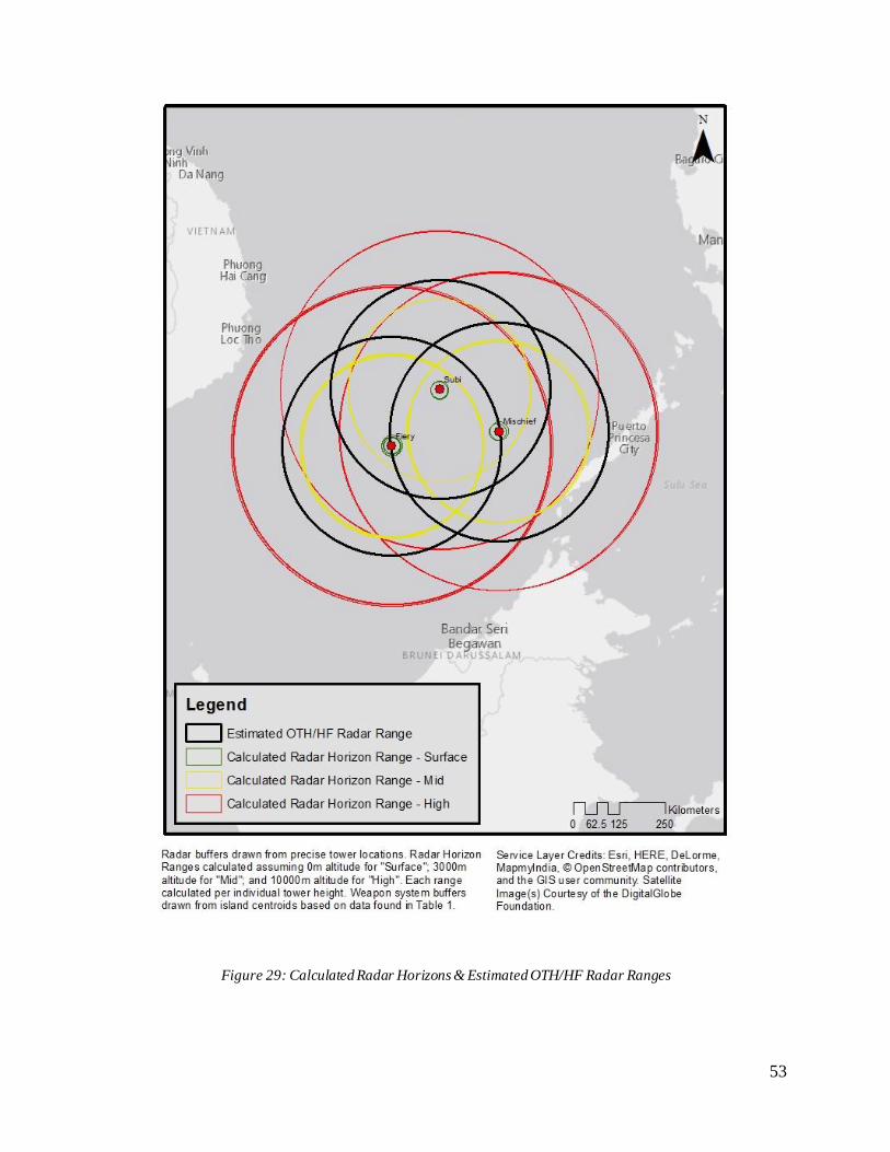
Figure 29: Calculated Radar Horizons & Estimated OTH/HF Radar Ranges .............................. 53
Figure 30: The Narrow Margins of OTH/HF Ranges with Fiery Cross Reef Inset ...................... 55
Figure 31: Radar Horizons Calculated using CSIS/AMTI Assumed Tower Height .................... 58
Figure 32: Radar Horizon Range Discrepancy at Surface Altitude .............................................. 60
Figure 33: Radar Horizon Range Discrepancy at Mid Altitude .................................................... 61
Figure 34: Radar Horizon Range Discrepancy at High Altitude .................................................. 62
Page 9
ix
List of Tables
Table 1: PRC Weapon System Ranges ......................................................................................... 28
Table 2: Tower Imagery Locations ............................................................................................... 34
Table 3: Tower Height Measurements and Height Calculations .................................................. 40
Table 4: Radar Horizon Ranges at Various Altitudes ................................................................... 42
Table 5: Ranges Derived from Average (Mean) Tower Height ................................................... 44
Table 6: Radar Horizons of CSIS/AMTI Assumed Tower Height ............................................... 57
Table 7: Observable Area Differences Per Tower ........................................................................ 59
Table 8: Observable Area Differences From Tower Locations .................................................... 63
Page 10
x
Acknowledgements
My studies in Geospatial Science began through conversation with Dr. Darren Ruddell,
who encouraged my nascent interest in geography and opened my eyes to the world of data
science. Dr. Steven Lamy highlighted the importance of Geospatial Science as a complement to
my study of International Relations and provided guidance and opportunities for this technical
skill to flourish in my native field. Dr. Steven Fleming in turn prompted my decision to begin a
Master’s program in Geospatial Information Science & Technology, and provided invaluable
mentorship throughout my studies, research, and career development. Work with Armament
Research Services cultivated a spirit and tradecraft of adventurous, complex problem solving.
These mentors have shaped my academic success throughout university and post-graduate life.
Dr. Steven Fleming’s guidance as advisor to this thesis was additionally invaluable, as
was that of committee members Dr. John Wilson and Dr. Andrew Marx. It did not hurt to have
the advice and awareness of two veterans of the United States Army and United States Air Force
officers in Dr. Fleming and Dr. Marx, graduates of their respective service academies to boot.
Dr. John Wilson’s wealth of knowledge, both of world geographic features as well as geospatial
technologies was instrumental in many minor details throughout. Thanks is also due to Dr.
Andrew Coe, whose courses inspired this research topic.
This project attempts to increase the accuracy of published data and reportings of the
Center for Strategic & International Studies, and so great appreciation must be shown to their
prompt email responses and help in locating mutual data sources to aid in an accurate analysis.
The DigitalGlobe Foundation is likewise acknowledged for their generous, timely, and cost-free
imagery provision.
Page 11
xi
Abbreviations and Terminology
A2AD Anti-Access & Area Denial
ADIZ Air Defense Identification Zone
AMTI Asian Maritime Transparency Initiative
China People’s Republic of China (PRC)
CSIS Center for Strategic & International Studies
DEM Digital Elevation Model
GIS Geographic Information System
HF High Frequency
LOS Line-of-Sight
NDL Nine-Dash Line
OTH Over-the-Horizon
PRC People’s Republic of China (“mainland China”)
RS Remote Sensing
SCS South China Sea
SSI Spatial Sciences Institute
Taiwan Republic of China
USC University of Southern California
Page 12
xii
Abstract
The People’s Republic of China’s (PRC) militarization of artificial islands in the South China
Sea (SCS) represents a challenge to security of, and freedom of navigation in, international
waters. Static defenses on these islands enhance Anti-Access and Area Denial (A2AD) efforts,
allowing de facto sovereignty in the area sustained by successful radar coverage. While many
A2AD tools may not be measured without direct access to the product, conventional radar
structure heights may be measured remotely, allowing for indirect measurement of an
adversary’s radar range. Though estimates for these ranges have been published by various
defense thinktanks, this study builds on shadow analysis literature to perform more accurate
measurement and projection of radar ranges through use of remote sensing and trigonometry
applied to imagery of SCS radar construction in late 2017.
This study uses shadow analysis to measure radar tower heights combined with radio
wave propagation equations to provide a viable alternative to rule-of-thumb estimation. This
novel methodology is tested on radar arrays identified by the Center for Strategic and
International Studies (CSIS) on three key islands in the SCS’s Spratly Islands. Radar horizon
range measurements provide a detailed analysis of radar coverage at various altitudes, showing
that previously published estimates can differ from bespoke analysis by more than double. The
study quantifies average range of radar arrays on artificial islands created by the PRC, finding
the average radar to reach radar horizon in 23.82 km distance at 0 m altitude; equal to 249.47 km
at 3,000 m, or 435.81 km at 10,000 m, respectively.
Page 13
1
Chapter 1 Introduction
This study combines traditional Remote Sensing (RS) imagery analysis with Geographic
Information Systems (GIS) to measure the radar horizons of a select group of radar structures
identified by the Center for Strategic and International Studies (CSIS) and their Asian Maritime
Transparency Initiative (AMTI). The radar structures, or radar towers, are located on artificial
islands and reclaimed land in the South China Sea (SCS) by the People’s Republic of China
(China) in the 2010s.
Radar serves a vital role in China’s territorial defense and Anti-Access (A2) and Area
Denial (AD) tactics currently of concern to strategic thinkers. The radio waves used by radar are
nonetheless limited by line-of-sight (LOS) and, therefore, radar vision is limited by positioning.
The placement – and especially heights – of radar systems has a powerful effect on LOS and is
vital to measuring radar range. Assessing these positions and heights is difficult as a function of
their military classification and the limited publishing of defense information on system
capabilities. The CSIS and AMTI have previously identified radar ranges for these towers using
common industry estimates. This study tests a method for more accurate estimation of radar
ranges, as necessary for analysis of the PRC’s A2AD capabilities, strengths, and weaknesses in
the SCS.
1.1. Motivation
This project parallels the recent changes in the SCS, the geostrategic effects of
militarization of new Chinese islands, and the increased accessibility of RS to the public as an
open source analysis community. Chinese territorial claims, outlined by the Nine-Dash Line
(NDL) have taken an adversarial nature against rival claims with various other Southeast Asian
states. Reinforcing Chinese claims, various artificial islands have been built of reclaimed land on
Page 14
2
the existing sites of reefs and atolls, complete with military infrastructure. With commercial and
open source satellite imagery available at limited or no cost, a new age of imagery analysis by
private citizens has come to rival commercial and government intelligence outfits.
To this end, there is opportunity to enhance public reporting by the think tanks such as
the Center for Strategic and International Studies’ Asian Maritime Transparency Initiative
(AMTI). While most of the military tools discussed by CSIS/AMTI are out of reach under the
supervision of a foreign military, radar structure heights, and, therefore, ranges, are available for
measurement via readily accessible RS imagery. Radar is the first line of A2AD defense, and
understanding its range is vital for informing the public about an adversary’s true military
capabilities. Therefore, the proposed study takes a novel approach that combines open source
GIS and RS methods and data to solve a relatively overlooked problem that experts project to be
at the core of future US military confrontation.
1.2. Research Objective
This thesis examines the radar coverages of China’s new radar stations built in the South
China Sea, and reviews the coverage compared to other known weapon systems and to radar
coverage estimates from CSIS/AMTI publishing. This project measures radar tower heights via
shadow analysis; uses these height measurements to measure radar horizons from each tower at
various altitudes; compares these coverages with weapon system ranges previously identified on
the islands to search for strengths and weaknesses in coverage overlap; and, finally, compares
these ranges to CSIS/AMTI data, to evaluate the discrepancy between the study’s calculations
and estimates.
Page 15
3
1.3. Scope & Data
This project focuses on a limited – but key – portion of published estimates by
CSIS/AMTI. The study addresses these estimates in reference to identified radar structures on
newly dredged Chinese islands in the Paracel and Spratly island chains, shown in Figure 1. To
increase the accuracy of published estimates, this study calculates radar ranges for structures on
the “Big Three” islands in the Spratly chain which CSIS/AMTI has confirmed have new radar
stations: Mischief Reef, Fiery Cross Reef, and Subi Reef (AMTI).
Figure 1: GIS and RS Publishings of Ranges and Radar Tower Identification. Source: AMTI 2017
Page 16
4
While this study proposes a method applicable to any potential radar tower visible in
aerial or satellite imagery, the focus of this project is tailored to a selection of militarized
artificial islands in the SCS occupied by China. Out of seven of these features in the furthest
island chain, the Spratlys, three are distinguished by a substantially larger reclaimed area, level
of infrastructure, and military activity. These “Big Three” are comprised of Mischief Reef in the
north of the Spratlys, Fiery Cross Reef to the west, and Subi Reef to the east. They form a
triangle around all but one of the other seven islands (Johnson Reef South, Hughes Reef, and
Gavens Reef inside, with Cuarteron Reef outside). According to CSIS/AMTI and other
researchers cited throughout this work, the “Big Three” form the core of a potential PRC military
launch pad while providing defensive coverage for interior islands. The only island in the chain
outside the “Big Three” triangle is Cuarteron Reef, where numerous radar arrays allegedly make
this a forward reconnaissance base (Lee 2015). Imagery from CSIS of these artificial islands is
provided below in Figures 2 - 4.
Figure 2: Mischief Reef, July 2016. Source: CSIS Island Tracker.
Page 17
5
Figure 3: Fiery Cross Reef, June 2016. Source: CSIS Island Tracker.
Figure 4: Subi Reef, July 2016. Source: CSIS Island Tracker.
Page 18
6
1.3.1. Data
Analysis for this study has been provided by CSIS, including data of digitized points
based on imagery provided by GeoEye, publicly available for academic study and published to
ArcGIS Online, as well as to the CSIS website in .kmz format, though of poor quality. Imagery
for this analysis was provided by the DigitalGlobe Foundation, without which this study could
not be performed.
Page 19
7
Chapter 2 Background and Literature Review
PRC island building in the SCS is an attempt to create de facto sovereignty in the region using
longstanding but unrecognized territorial claims. Control over the SCS can provide the PRC
assured access to the resources held within its boundaries, give buffer against forces invading the
homeland, and open routes of communication, trade, and surveillance. Territorial claims like
China’s often follow historic precedent or cite historic need, while tactics for control over
territory adapt to a given state’s current technology and potential adversaries. The modern tool of
radar finds itself as a prime facilitator of territorial defense, especially considering recent shifts
toward modern asymmetric defense strategies, including A2AD. Radar relies greatly on LOS
vision for the transmission and reception of radio signal, and therefore is constrained by physical
geometry and the curvature of the Earth. Identification of radar infrastructure is a necessary
pursuit of counter-A2AD strategy and relies greatly upon RS tactics. Gaps remain in the RS
evaluation of radar heights to measure radar LOS range.
This chapter first describes the history of the region and China’s relationship w ith the
territory in question. This is followed by a discussion of claimants and the contest of territorial
rights to the SCS. The nature of A2AD is then discussed within the context of the SCS. Radar as
a tool of A2AD is examined. Review of existing RS and GIS radar analyses completes the
chapter, to highlight the research already existing within the field.
2.1. The South China Sea in History and International Relations
As the issue of territorial claims in the SCS is fundamentally a concern of international
relations, viewing it through a social science lens can offer great clarity to the root of the
problem. In this light, the SCS is much like other bodies of water bordered by multiple states. It
is a shared space, but this space can be used for cooperation or competition. The SCS’s
Page 20
8
geopolitical role as an international space has therefore been analyzed in comparison to the
politics of other shared seas, with a range of resulting models. The US-Caribbean model
represents a system of disinterested hegemony (Kaplan 2014), whereby China casually controls
and maintains the politics of the region through indirect means. The Germany-North Sea model
focuses on the nature of limited sea-lane access through the body in wartime (O’Mara 2013), and
highlights China’s concern for access to the SCS, leading to a more confrontational and risk-
tolerant attitude in the region. The Europe-Mediterranean model supposes a region of economic
competition despite shared culture (Evers 2013) and assumes that international consensus can be
reached for mutual maintenance and access in the SCS. While the prevailing literature cited in
this section and Section 2.2 take a tone more reminiscent of the first two models, there is hope
that a more cooperative outcome is possible. All these theories, however, pivot around economic
objectives and security concerns based on historical precedent. PRC development of artificial
islands in the SCS is therefore integrally related to the exploitation and defense of the territory.
2.1.1. Access to Trade & Resources
Chinese contact, and trade, with the remainder of the world has traditionally flowed
through the SCS. China has long “perceived themselves dominant” over the sea lanes that ran
south through the Strait of Malacca, despite distance and the development of modern rivals in the
region (Souza 2014). Chinese trading through the SCS dates from 500 BCE (Gungwu 1954) and
was maintained as what “may well be the most enduring maritime trade route in history” despite
intermittent closure during wartime (Gao & Jia 2013). A great manner of wealth has consistently
traveled between civilizations along this route, where “the Chinese exchanged their silks and
other manufactured goods for luxury goods like ivory, pearls, tortoise shells, kingfisher and
peacock feathers, rhinoceros horns and cinnamon and scented woods” in preindustrial eras, to
Page 21
9
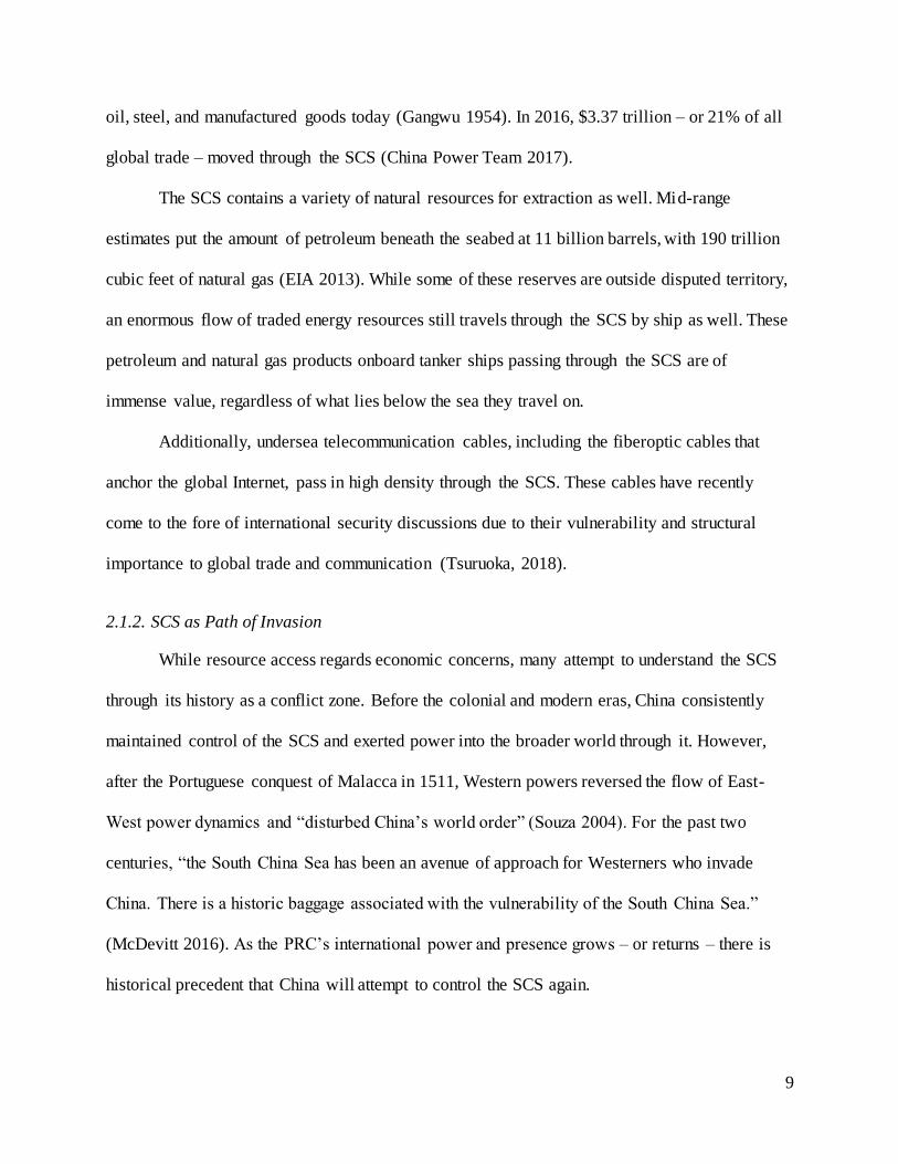
oil, steel, and manufactured goods today (Gangwu 1954). In 2016, $3.37 trillion – or 21% of all
global trade – moved through the SCS (China Power Team 2017).
The SCS contains a variety of natural resources for extraction as well. Mid-range
estimates put the amount of petroleum beneath the seabed at 11 billion barrels, with 190 trillion
cubic feet of natural gas (EIA 2013). While some of these reserves are outside disputed territory,
an enormous flow of traded energy resources still travels through the SCS by ship as well. These
petroleum and natural gas products onboard tanker ships passing through the SCS are of
immense value, regardless of what lies below the sea they travel on.
Additionally, undersea telecommunication cables, including the fiberoptic cables that
anchor the global Internet, pass in high density through the SCS. These cables have recently
come to the fore of international security discussions due to their vulnerability and structural
importance to global trade and communication (Tsuruoka, 2018).
2.1.2. SCS as Path of Invasion
While resource access regards economic concerns, many attempt to understand the SCS
through its history as a conflict zone. Before the colonial and modern eras, China consistently
maintained control of the SCS and exerted power into the broader world through it. However,
after the Portuguese conquest of Malacca in 1511, Western powers reversed the flow of East-
West power dynamics and “disturbed China’s world order” (Souza 2004). For the past two
centuries, “the South China Sea has been an avenue of approach for Westerners who invade
China. There is a historic baggage associated with the vulnerability of the South China Sea.”
(McDevitt 2016). As the PRC’s international power and presence grows – or returns – there is
historical precedent that China will attempt to control the SCS again.
Page 22
10
2.2. South China Sea Border Claims
The importance of the SCS is evident through the contest of claims over it. China’s claim
in the SCS does not exist in a vacuum, as Vietnam, the Philippines, Malaysia, Taiwan, and
Brunei share both legitimized and dubious claims to the area as well. These claims have been
summarized in Figure 5 below by the Wall Street Journal (Page 2016).
Figure 5: Competing Claims for the SCS. Source: Wall Street Journal, 2016
2.2.1. China’s Claim
Today, the PRC’s SCS island building has been correlated with heightened reference to
the Nine-Dash Line territorial claim. The Nine-Dash Line (NDL) claim originates from 1930 (Li
& Li 2003) as a solid, not dashed, “U-Shaped Line” to standardize maps made in the nation. This
solid boundary showed Chinese territorial control over much of the SCS, far beyond the standard
200 nmi boundary permitted by the future United Nations’ Convention on the Law of the Seas
(UNCLOS). Nonetheless, the first dashed line was published later without international dissent
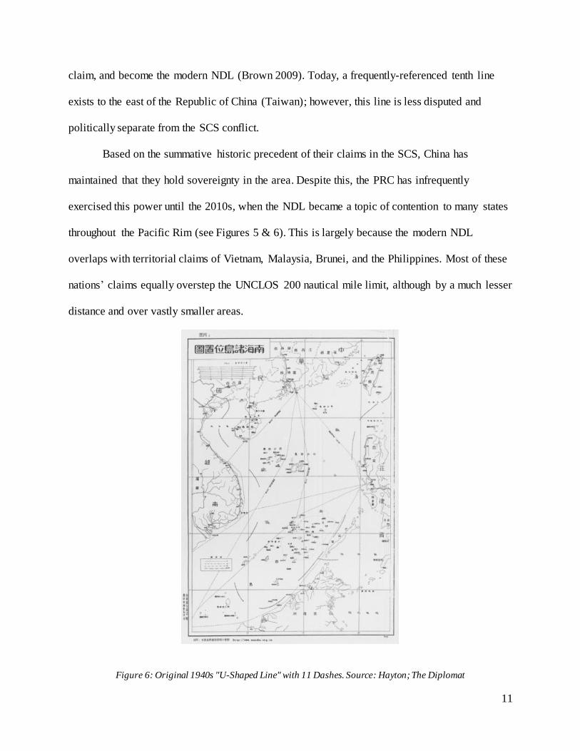
or comment, with an eleven-dashed line released over 1947 and 1948 (see Figure 6). The eleven-
dashed line was later reduced to nine dashes, to reduce infringement on Vietnam’s maritime
Page 23
11
claim, and become the modern NDL (Brown 2009). Today, a frequently-referenced tenth line
exists to the east of the Republic of China (Taiwan); however, this line is less disputed and
politically separate from the SCS conflict.
Based on the summative historic precedent of their claims in the SCS, China has
maintained that they hold sovereignty in the area. Despite this, the PRC has infrequently
exercised this power until the 2010s, when the NDL became a topic of contention to many states
throughout the Pacific Rim (see Figures 5 & 6). This is largely because the modern NDL
overlaps with territorial claims of Vietnam, Malaysia, Brunei, and the Philippines. Most of these
nations’ claims equally overstep the UNCLOS 200 nautical mile limit, although by a much lesser
distance and over vastly smaller areas.
Figure 6: Original 1940s "U-Shaped Line" with 11 Dashes. Source: Hayton; The Diplomat
Page 24
12
Despite the NDL territorial claims, China has elaborated very little on the legitimacy of
its sovereignty over the area. This elaboration is necessary to ground the claim in legitimate
international law. One source of potential legitimacy commonly referenced is historical
precedent of the territorial claim. Li & Li (2003) outline that China has nearly fulfilled the
requirements to claim “historic waters” as outlined by the International Law Committee by the
United Nations Secretariat in 1962, but has stopped short of the processing this claim through
any international body. Like all other potential methods of acquiring claim legitimacy, the
“historical waters” claim has nonetheless not been officially stated for international review.
Much like the purposeful vagueness of the NDL, whose dashes leave cartographers in confusion,
China has made “no official claims other than a claim to ‘sovereignty’ [in the SCS]… No
spokesman has ever gotten up and said, ‘the official position of the government of China is X.’”
This hamstrings the international community from resisting the PRC’s SCS takeover, as the PRC
has not “even [published] a credible maritime entitlement claim that [one] could protest as
excessive” (McDevitt 2016). Overall, this fails to define sovereignty, territorial control, and
legitimacy in the SCS. The situation is therefore ripe for land grabs and de facto annexation.
2.2.2. Other Claimants
Other regional claimants have strong interests – both for and against – the enforcement
China’s NDL. Taiwan backs China’s NDL due to similar land claims on Taiping Island and has
supported China’s claims in international court (see PDCC 2015). Considering historic
“acquiescence” to China’s claim by neighbors (Zhao 1999), the government of Taiwan considers
“the entire area within the U-shaped line to be China’s historical waters” (Cheng-yi 1997).
Taiwan even often references the original phrasing – “U-shaped line” – rather than the newly
termed “Nine-Dash Line” (Wang 2010).
Page 25
13
In 2013, a legal battle initiated by the Philippines became a topic of concern for SCS
claimants and neighbors. In the case, international courts sought to establish a precedent based
on UNCLOS jurisdiction over the SCS. In 2016, the Philippine plaintiffs won the case, but many
supporters remained disappointed with the outcome. Jurists have complained that no real result
was reached despite the Philippine victory, as Chinese economic pressure effectively nullified
any enforcement of the decision, leading the Philippines to pull back from the territory rather
than exert their legitimate claim (Sofaer 2016).
Vietnam has faced a similar situation in previous decades, but with more violent results.
Vietnamese claims to the SCS were dampened in 1974 with China’s forcible removal of
Vietnamese forces from the Paracels, and again in 1988 as the Chinese “sank three Vietnamese
supply ships, killed seventy-two Vietnamese, and captured nine” in the Spratlys (Gallagher 1994,
174). Despite this, Vietnam has maintained quiet opposition to Chinese encroachment,
encouraged by the US and others to express that, “even though there is not [military] parity, the
message gets across to Beijing that their changes to the status quo [in the SCS] are going to be
met with other changes that are against their interest” (Cooper 2016). Vietnam has thus found
itself allying with PRC-opposing nations on the issue.
In sum, these claims have been specifically identified in relation to natural resource
locations, as shown in Figure 7.
Page 26
14
Figure 7: Competing Claims and Natural Resources. Source: The Brookings Institute; Reuters.
2.3. Anti-Access & Area Denial
If PRC island-building fits the explanation of a territorial control attempt within its NDL,
the strategy of control and defense of the claim is the next concern. Experts largely agree that the
threat posed by Chinese military buildup in the SCS is that of an Anti-Access, Area Denial
(A2AD) strategy. A2AD is a topic of increasing research in recent years, as described in this
section. To this end, this study draws its relevance from the importance of understanding and
countering the described A2AD strategy, and how geospatial techniques may be used for this
purpose.
First, there is contention with use of the popular phrase A2AD. The concept of A2AD is
not new, nor are the tactics currently used for A2AD a “change [in] the nature of modern
warfare” (Davin 2013, 5). The only unique aspect of A2AD is current technological trends
Page 27
15
applied to age-old asymmetric tactics of threatening supply and communication routes and
making opposing intervention risky. Nonetheless, “the use of the A2AD framework is a critical
tool for looking at the operational problem posed by China’s military buildup because the US
must [assure] allies that it will maintain access” to sea lanes and trade routes (Davin 2013). To
acknowledge this fact, this thesis will therefore use the term A2AD to describe defensive
asymmetric tactics currently employed by China, for the sake of clarity with existing literature.
The most comprehensive explanation of A2AD toolsets, strategies, and their
countermeasures was compiled by Krepinevich (2003) in a manuscript delivered to Congress.
The work references changing military tactics as the US entered a new phase of warfare in the
21st Century, detailing the asymmetric tactics of US enemies brought about following the
overwhelming US victory in Iraq in 1991. As this trend has continued even up through the
current day, the tactics have become more defined, and taken a more deliberately geopolitical
focus. As A2AD centers on the control of geographic territory and the placement of defenses
within it, the strategy is inevitably built on geospatial units, available for geospatial measurement
and analysis: the areas of territory defended, the zones of coverage provided by A2AD systems,
and the distances between defenses both static and mobile. A2AD’s geopolitical nature therefore
avails itself of a GIS frame of investigation.
The need for GIS analysis of A2AD capabilities is evident in the social science realm’s
growing concern for it over the decades after Krepinevich’s (2003) publication. McCarthy
(2010) expanded upon Krepinevich’s developments nearly a decade on, after the second invasion
of Iraq in 2003. He noted an increase in A2AD tactics in the mainstream of anti-US states,
confirming Krepinevich’s (2003) observation that a new wave of A2AD tactics were on the rise
throughout countries traditionally opposed to the US and the West. The current US perspective
Page 28
16
on A2AD is additionally outlined by in periodical publications rather frequently. Cheng (2014)
discusses the specifics of Chinese interests and US policy objectives against them. Military
historians likewise relate Chinese A2AD efforts in the SCS to German attempts at North Sea
domination in the Battle for Britain (O’Mara 2013) and underscore the Chinese strategic
emphasis on airspace control as a source of A2AD.
The effects of A2AD defenses have powerful strategic and geopolitical effects, with
some researchers even encouraging US planners to “abandon or lessen reliance [on attempts at]
Air Superiority over Mainland China” due to the high cost of penetrating Chinese air defense
structures – radar foremost among them (Overcash 2010). This advice comes with geographic
reference, but little geospatial clarity, however. Especially on the issue of radar, the GIS analysis
dearth has been highlighted as published discussion of PRC radar capabilities focus on smaller
and smaller geographic scales, without touching on measurable specifics. For example,
testimony before Congress has detailed the Chinese need for radar extension into the SCS to
improve China’s “ground-based radars [that] provide overlapping coverage of coastal areas”
(O’Rourke 2017; Overcash 2010), but offered little calculable evidence. The literature generally
agrees that Chinese A2AD is focused on air power and anti-ship efforts, but almost all A2AD
tools can be visualized or measured in a geospatial context. Whatever the A2AD tool of focus,
mounting a defense relies on “the first step… the detection of a potential target” via radar
systems (Davin 2013). This highlights the importance of radar as a force multiplier, and the great
danger it poses to the PRC’s potential adversaries. According to Admiral Mike McDevitt, USN
(Ret.), “China [is] now, potentially for the first time, achieving defense and depth” in the SCS.
Anti-ship and anti-air surveillance “will give them an opportunity to monitor [threats] throughout
the SCS. If you chose to use the SCS as an avenue of approach, it would be an interesting go”
Page 29
17
(2016). But what avenues are and are not available is far too important a question for regional
generalization. A geospatial analysis is needed of A2AD tools, or at least a model of how such
calculations might be performed.
Overall, US interests require that it resists Chinese A2AD efforts (Davin 2013; Hoyler
2013; Cheng 2014; McCarthy 2010; Gerson 2011). The most cost-effective method of inhibiting
Chinese A2AD is to eliminate the first step in their anti-ship and anti-air “kill chain”: ground-
based radar surveillance and targeting systems (Davin 2013; Overcash 2010). To do so will
require a thorough understanding of the problem that is only available through investigation with
a GIS framework, and with an informed understanding of radar itself.
2.4. Radio Propagation and Radar Line of Sight
Radar operates through transmitting radio waves across an area, which reflect off objects
and return to a receiver. The receiver then calculates the location, size, and potential movement
of the reflecting object based on the returned signal (Skolnik 2007). In many aspects, these radio
waves operate much like visible light, and are limited in similar ways to line-of-sight vision. As
the Earth is not flat, the curvature of the Earth bends away from a viewer and removes it from
line-of-sight, which changes dependent on one’s height (Haslett 2008). Beyond the horizon,
electromagnetic waves struggle to pass through the dense bulge of the Earth’s sphere and are
rendered invisible. Simply put, “distance to the horizon depends on your height,” and the taller
the viewer, the further they can see. In terms of radar, the taller the radar structure, the further
away it can observe.
2.4.1. Radar Height as Measure of Range
Height therefore is the dominant factor in establishing visible range for both visible light
and radio waves. Via the Pythagorean Theorem, the theoretic distance to the visible horizon is
Page 30
18
seen in Equation 1 and illustrated by Figure 8 (for a full catalogue of equations used in this
study, see Appendix D).
𝐷ℎ ≈ √2 ∙ 𝑅 ∙ 𝐻 (1)
Figure 8: Visual Depiction of Horizon Trigonometry. Source: Plait 2009
where 𝐷ℎ is the distance to the visible horizon, R is the radius of the earth, and H is the height of
the viewpoint from the surface of the earth. This equation can be simplified to Equation 2, when
using an average radius of the Earth to account for slight variation in its curvature at 6371 km:
𝐷ℎ ≈ 3.57 ∙ √𝐻 (2)
where 𝐷ℎ is measured in kilometers, and H is measured in meters (NAVAIR 2013, Chp 4;
Haslett 2008, 33; Valtr & Pechac 2005, 491). These equations refer to the exact lines-of-sight
one might have with human vision. However, various factors affect electromagnetic waves in the
radio spectrum differently than the visible light spectrum. In fact, atmospheric conditions and the
ability of radio waves to bounce constructively create a “geoclimatic factor,” K, that increases
radio wave range with a multiplier of 1.33, or four-thirds (Bacon, 271; Haslett 2008). Valtr &
Pechac (2005) and other researchers have examined changes in K at various altitudes and
Page 31
19
environmental conditions. The effect of K increases the range of radio waves beyond the horizon,
creating a bend for radio waves that is “very slight, but… in the same sense as the curvature of
the Earth… [t]he overall result is that the radio horizon is further than the visible horizon”
(Haslett 2008). Thus, Equation 2 can be adjusted to Equation 3 as follows to account for K when
measuring with radio waves:
𝐷ℎ ≈ 4.12 ∙ √𝐻 (3)
All of these equations, however, only measure a radio line-of-sight maximum, or radar horizon,
at the surface of the Earth. To calculate the maximum distance line-of-sight to an object of non-
zero height, Equation 4 is used (NAVAIR 2013):
𝐷𝑚𝑎𝑥 ≈ 4.12 ∙ (√𝐻𝑂𝑟𝑖𝑔𝑖𝑛 + √𝐻𝑇𝑎𝑟𝑔𝑒𝑡) (4)
This equation will be used to measure radar ranges based on radar height data, as discussed later.
It should equally be noted that Equation 4 may be solved for the unknown height of a given
visible object at known distance, using Equation 5 as follows.
𝐻𝑈𝑛𝑘𝑛𝑜𝑤𝑛 ≈ (𝐷𝑚𝑎𝑥
4.12− √𝐻𝐾𝑛𝑜𝑤𝑛)
2
(5)
As the equation is not a direct geometric measurement but rather a mathematical approximation,
the units used in Equation 4 are still valid.
2.4.2. Radar Beyond Line of Sight
Radio signals can also be bounced off the ionosphere in the upper atmosphere and
reflected back down to Earth beyond the traditional LOS-method of conventional radar. This
technique, known as Over-The-Horizon (OTH) or High Frequency (HF) radar, is “quite
attractive for the radar observation of areas (such as the [surface of the] ocean) not practical with
Page 32
20
conventional microwave radar” (Skolnik 2007). Although OTH/HF radar can surveil at ranges
up to 2000 nmi, it requires large arrays for both transmitters and receivers which are strikingly
different in construction and easily identifiable in aerial imagery. These are standardly
constructed either as large “elephant cage” ring structures, or in rowed pickets of small antennae
rather than the clear domed towers of conventional ground-based radar structures. Additionally,
OTH/HF radar is considered to have a lower resolution and is not always suitable for identifying
aircraft or for the detailed targeting of surface vessels (Nathanson 1991, 19). OTH/HF radar
additionally has distant minimum ranges. Other forms of extending radar range like the OTH/HF
method have been researched for some time, focusing on environments that might affect the
coefficient K, such as weather or other atmospherics (Booker 1946; Rogers 1957). In terms of
the SCS, there is a speculation of a possible OTH/HF “elephant cage” systems on various
islands, first identified on Cuarteron Reef (AMTI). This study will focus on traditional
conventional radar tower systems nonetheless due to the impracticality of estimating OTH/HF
radar without direct access to the system. As it does not follow clear rules for use, like
conventional radar’s reliance on LOS, it is much more difficult to estimate or calculate remotely.
2.5. Monoscopic Photogrammetry for Shadow Analysis
The range of radar is dependent on the sensor’s height, as discussed above. An object’s
height may be measured using its shadow length, based on geometry of the Sun’s angle and the
object’s location on Earth – a geospatial approach. Because aerial and orbital imagery acquired
through remote sensing techniques rarely capture sidelong views of buildings, “an obvious
starting point for height estimation is the sun shadow” (Wegner et al . 2014). While this
estimation can be performed more easily with multiple images of the same object captured from
different angles (stereo photogrammetry), shadow analysis is the prime method when dealing
Page 33
21
with a single image or single image angle (monoscopic photogrammetry), which is most useful
in the limited data environment of adversarial military analysis. In the presiding literature, the
term “shadow analysis” in both stereo and monoscopic photogrammetry is used to differentiate
height estimation efforts from other aspects of photogrammetry.
A basic outline of the monoscopic photogrammetric method of shadow analysis can be
found from Cordova (2005). Likewise, Adeline (2013) provides a review of various RS shadow
measurement uses, identification methods and algorithms, and physical constraints. While
property-based methods of shadow analysis rely on spectral imagery to evaluate radiance and
reflectance of shadows, this thesis focuses more heavily on model-based shadow analysis. This
method uses a geometric and physical approach to shadow analysis and aims to measure objects
and their cast shadows; however, it requires situational information (angle of the sun, shadow
surface orientation, etc.) as opposed to wider spectral bands (Adeline et al. 2013; Al-Najdawi et
al. 2012; Shao et al. 2011).
The model-based method is also better suited for extracting physical information about a
sensed object, such as height, through the trigonometric Equation 6 as follows (Larson 1993):
𝑥 tan 𝜃 = ℎ (6)
where x is the known shadow length, 𝜃 is the angle of the sun’s altitude (calculable from known
time and location on Earth, and often embedded in digital imagery), and h is object height. While
this method of height calculation is common in aforementioned research, McGlone (1994)
performs additional analysis using oblique angle viewpoints rather than right-angle trigonometry,
creating an automated shadow calculation and object identification tool.
Algorithms for shadow enhancement in aerial imagery (Liasis & Stavrou 2016) parallel
advancements in shadow detection with small-scale ground-based sensors (Al-Najdawi et al
Page 34
22
2012). Often, model-based studies are used to more accurately identify shadow location (Li et al
2005), while property-based methods provide more definite identification of shadow edges
(Nagao et al 1979) and objects within shadows (Shimoni et al 2011).
There is also a blending of both forms by which radiance data is used to make shadows
more identifiable for model-based analysis, while length identification is used to build better
parameters in property-oriented image classification. The heights of ice-ridges were measured by
Kwok (2014) using shadows from satellite imagery, with subsequent analysis by Miao (2016)
creating a system of image classification for ice-ridges using these shadow-to-height
measurements. One step further, Wegner (2014) use a variety of interferometric synthetic
aperture radar (InSAR) measurements in combination with sun shadow lengths to build high-
confidence object height estimations. Research has also been conducted into automated shadow
removal from imagery in open source products like Google Earth using these same techniques
(Guo et al. 2010; Kwatra & Dai 2012). Finally, Raju (2014) discusses issues with shadow
visibility when performing shadow analysis in image classification studies. In this regard, there
is a wealth of literature on shadow photogrammetry, though much is devoted toward image
classification rather than object detection, such as this thesis’s proposed application to radar
structures.
2.6. GIS Studies of Military Radar
The majority of radar-related GIS non-RS studies regard location optimization problems,
but still provide a baseline for how radar is measured by GIS in a military setting. Bell (2011) is
heavily cited for this application of GIS, reviewing missile defense alert structures. In the study,
alert radar coverages of targets are sought according to hierarchical target values, with free
position of radar structures. In essence, this allows for the planning of radar defenses based on
Page 35
23
known targets. Alkanat (2008), like others (e.g., Franklin et al 1994), applied similar methods as
Bell toward surface-to-air missile (SAM) coverage in Turkey. Using defined targets with
hierarchical value, Alkanat optimized locations for various SAM systems to ensure coverage.
Straitiff (2010) performed a location optimization analysis of similar optimization problems
using a less direct workflow. Staitiff’s study theorizes optimal geometries of coverage, bounds
this geometry to a target, and then performs adjustments to increase optimization within the new
boundaries. Gonsalves (2003) outlined the use of GIS and optimization of weapon system
interactions and provides geographic background to how radar in missile defense systems can
best communicate and coordinate.
Studies have also been performed based on existing radar stations and their real or potential
limitations. Kostic & Rancic (2003) modelled potential radar coverages in a virtual environment
as 3D analysis against known digital elevation model (DEM) data. This served to build
viewsheds and understand what a radar sensor might see in a given environment. Kucera (2004)
performed an analysis of Guam’s military radar stations with DEM data as well, creating
viewsheds of expected radio wave propagation from various radar towers. Zemmari (2012)
performed an analysis of potential maritime radar surveillance techniques with known radar
towers positions and developed a method of ship tracking through overlapping radar coverages.
Nonetheless, no research exists using GIS or RS measurement to estimate maximum radar
range via height calculation, as most mentioned studies either operate at too small a scale or too
specific a scope to discuss potential maximums bounded by Earth’s geometry. Additionally, few
articles evaluate enemy defensive structures, let alone attempt to estimate an adversary’s radar
heights. Almost all works focus on radar systems that are either hypothetical or to which the
researcher could potentially walk up in person. This thesis hopes to fill this gap, providing a
Page 36
24
novel approach within the realm of geospatial intelligence tradecraft which combines RS, GIS,
and geometry to solve radar range equations when radar heights are unknown.
Page 37
25
Chapter 3 Methodology
Existing literature does not provide a clearly analogous case methodology for the proposed
study. This may be in part due to the fusion of RS, raw math, and GIS into a single workflow.
Additionally, the study requires prerequisite knowledge and interest in RS, radio propagation,
and GIS. While Kostic & Rancic (2003) and Kucera (2004) focus on the role of elevation in
radar LOS (3D and 2D, respectively), their studies plot existing radar sensors through known
territory with potentially unlimited access to data and the sensors themselves, at ranges inside the
radar horizon. The true novelty of this thesis is the application of a similar investigation in an
environment without the issue of elevation change, but rather the issue of extremely limited
access to radar sensors and structures. Similarly, this thesis focuses on maximum radar ranges
limited by the curvature of the Earth rather than obstructions or radar signal loss.
The study area for this project consists of China’s “Big Three” land reclamation sites. RS
data was sourced from the DigitalGlobe Foundation, while CSIS/AMTI provided raw and
analyzed information regarding weapon systems and radar positions on the islands. Imagery
from DigitalGlobe was sourced in part from the GeoEye and WorldView satellite platforms.
These data were used for shadow analysis and trigonometric measurement of tower heights
within a GIS platform. Radar horizon calculations were then performed, adjusted for the
geoclimatic factor K. Data produced were measured as vector ranges of radar horizons for
comparison with various other weapon system ranges and with initial radar range estimates by
CSIS/AMTI. This methodology therefore provided an experimental approach to be used in later
studies of other radar sites in the SCS or similar environments.
Page 38
26
This study used a combination of techniques and manual measurements rather than an
automated, modelled approach. Results were analyzed based on shared coverage with other
A2AD systems, and subsequently evaluated the accuracy of CSIS/AMTI estimations.
3.1. Data
Three data categories were used in this methodology. Imagery data was used to perform
shadow photogrammetry. Weapon system ranges and radar range estimations from CSIS/AMTI
and other researchers was used as baseline coverages for comparison with those calculated in this
study. Geospatial data was largely created through this study, rather than used as an input, but
nonetheless served as vital reference.
3.1.1. Imagery
Imagery for this project was provided by the DigitalGlobe Foundation, ranging in
maximum ground sampling distance (GSD) for multispectral imagery at 1.24 to 1.84 m. The
georeferenced raster imagery was imported into ArcMap and overlayed with basemap imagery of
the region to ensure that any obvious georeferencing errors could be found and corrected.
Measurements taken from the imagery were measured in meters, with the imagery projected to
WGS 1984. Imagery can be seen in Figure 9 with higher scale inset to display resolution size.
Radar towers, previously identified by CSIS/AMTI as seen in Figure 10, were matched to
imagery in from the DigitalGlobe Foundation with recorded date and time. This information,
combined with geographic location, was calculated by the data provider and included with the
altitude angle of the sun in the imagery’s metadata.
Page 39
27
Figure 9: 1:1,250 and 1:23,000 Scale of Radar Array. Satellite image(s) courtesy of the DigitalGlobe Foundation.
Figure 10: CSIS Identification of Island Features, with Inlay of Radar Array.
Page 40
28
3.1.2. Weapon System Data
Various other weapon systems further down the A2AD “kill chain,” as discussed in
Chapter 2, were also vital for measurement in this study. As the tools enabled by radar warning
systems, they have an integral relationship with radar. The ranges of these tools and of radar
surveillance work together to match field of vision to field of response. The data in Table 1
describes the ranges of these tools as deployed by China in the SCS, some of which have already
been identified in the Spratlys and Paracels, and others yet suspected.
Table 1: PRC Weapon System Ranges
Reported Range Estimation, (Ashdown 2016; Gormley et al 2014; Kable Intelligence, CSIS/AMTI)
System Type Range
HQ-9 Surface to Air Missile 230km
YJ-62 Anti-Ship Missile 400km
J-10 Fighter Aircraft 550km
Radar High Frequency 300km
Radar Conventional 50km*
3.1.3. Geospatial Data
Geospatial shapefiles stored in .kmz format were also supplied via public hosting by
CSIS; however the data was deemed inappropriate for this project’s use due to its low quality.
Within the data was missing key island centroids, including Subi Reef, and appeared to be
derived from dated Google Maps GPS coordinates. These coordinates roughly note the location
of natural reef chain features, but do not accurately represent the new land reclamation features
on specific segments of often sprawling reefs. For this reason, visual centroid approximation was
manually created for the sake of developing island centroids, seen in Figure 11. This manual
Page 41
29
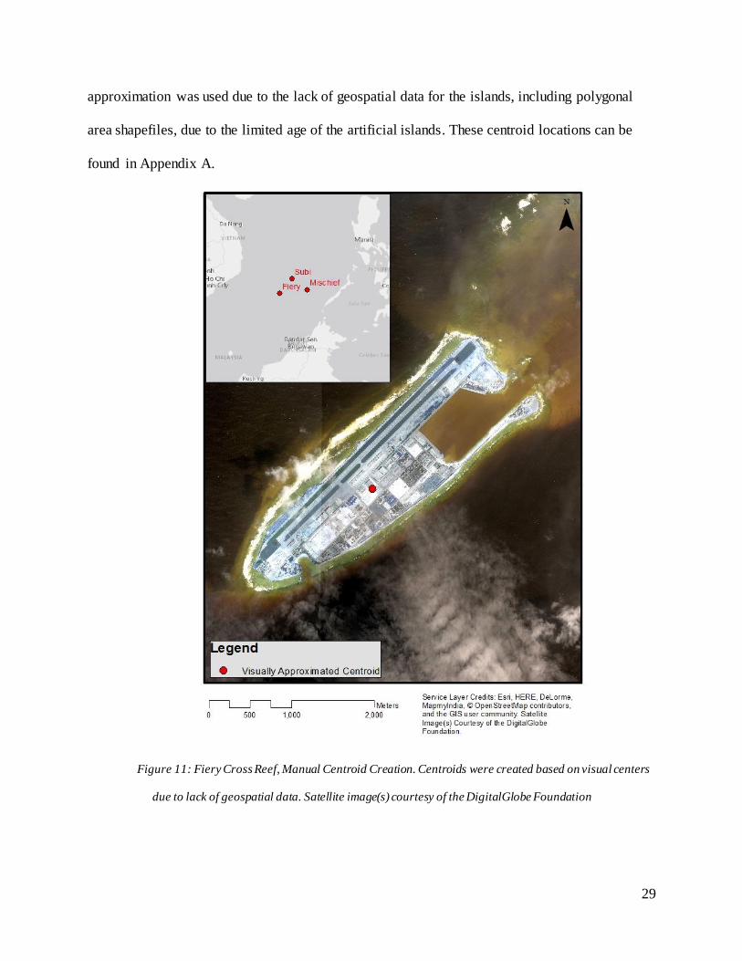
approximation was used due to the lack of geospatial data for the islands, including polygonal
area shapefiles, due to the limited age of the artificial islands. These centroid locations can be
found in Appendix A.
Figure 11: Fiery Cross Reef, Manual Centroid Creation. Centroids were created based on visual centers
due to lack of geospatial data. Satellite image(s) courtesy of the DigitalGlobe Foundation
Page 42
30
3.2. Procedure
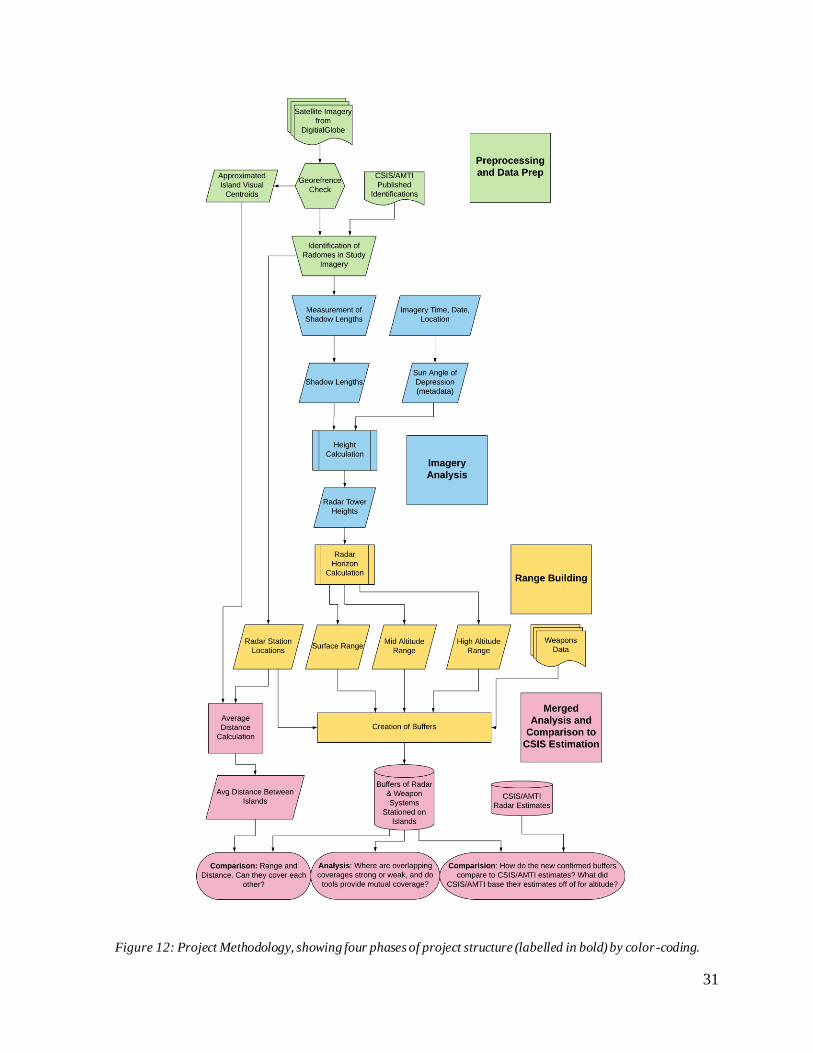
With these data, the project followed the research design detailed in Figure 10, whereby
data from CSIS/AMTI and the DigitalGlobe Foundation was re-analyzed for greater accuracy of
radar ranges using the notion of radar horizons. This project had four main phases: (1) data was
gathered, catalogued, and organized; (2) shadow analysis was performed to calculate radar
heights for each tower and these heights were then used to calculate radar horizons at various
altitudes; (3) these data were integrated into a GIS with new buffers created for other weapon
systems to match CSIS/AMTI publishing; and (4) these coverages were analyzed for comparison
with each other and with initial CSIS/AMTI radar range estimations.
3.2.1. Data Preparation and Preprocessing
Before the main analysis could be performed, available data was gathered and integrated
into a GIS (see procedural workflow in Figure 13). Satellite imagery from the DigitalGlobe
Foundation was overlaid against open source basemap data to ensure correct georeferencing.
This imagery was subsequently cross-referenced with CSIS/AMTI identification of radar array
locations as seen in Figure 10. Centroids for the data were needed, but could not be gathered
from existing sources and were therefore created manually as discussed below.
Radar array zones and their locations were matched and marked in the data for
subsequent analysis (see Figure 14), with GPS coordinates recorded in Microsoft Excel
spreadsheets for quick integration into any GIS or RS software system. Red, Green, and Blue
light bands embedded in the imagery were also adjusted manually to enhance visibility of each
individual shadow for the measurements that followed.
Page 43
31
Figure 12: Project Methodology, showing four phases of project structure (labelled in bold) by color-coding.
Page 44
32
Figure 13: Data Preprocessing and Integration Model
Figure 14: Zone FC2. Compare to Figure 10. Satellite image(s) courtesy of the DigitalGlobe Foundation.
Page 45
33
Each zone of radar arrays identified by CSIS/AMTI was examined and confirmed to be a
conventional radar tower array rather than an “Elephant Cage” or antenna picket OTH/HF
system. In total, this left six relevant zones, as identified by Figures 15, 16, and 17. Red-marked
“Radar/Sensor Array” zones not included depicted OTH/HF radar systems. In total, these zones
identified 13 individual radar towers for measurement. Each zone can be viewed individually in
Appendix B.
Due to the high volume of data provided by the DigitalGlobe Foundation, imagery that
did not contain relevant sites was removed from the GIS to increase processing speed.
Additionally, panchromatic imagery was discarded due to the ease in identifying shadows with
the visible spectrum. This reduced the imagery load from nearly 50 GB to below 0.5 GB,
including relevant shapefiles for georeferencing and image tile schemes; however, this also
removed higher resolution imagery which may have been useful for purposes other than shadow
detection (see Appendix A). Towers and their sites identified by this process are listed in Table
2.
3.2.2. Imagery Analysis
With the imagery prepared and catalogued, and each individual radar tower plotted by
GPS coordinates, shadow analysis was then performed, as articulated by the workflow in Figure
18. This methodology uses Equation 6 as described in Chapter 2 to calculate tower heights from
satellite imagery from Worldview 3, Worldview 4, and GeoEye 1 sensor platforms provided by
the DigitalGlobe Foundation.
Page 46
34
Table 2: Tower Imagery Locations
Tower ID
Zone
ID Island Satellite Image ID Tile Latitude (m) Longitude (m)
01 FC1 Fiery Cross Reef WV03 105001000D959600 R1C2 12,567,841.05 1,069,124.62
02 FC2 Fiery Cross Reef WV03 105001000D959600 R2C2 12,568,344.31 1,068,654.97
03 FC2 Fiery Cross Reef WV03 105001000D959600 R2C2 12,568,401.71 1,068,674.30
04 FC2 Fiery Cross Reef WV03 105001000D959600 R2C2 12,568,451.38 1,068,690.07
05 FC3 Fiery Cross Reef WV03 105001000D959600 R2C1 12,565,786.80 1,067,039.70
10 S1 Subi Reef GE01 10400100355E1900 R2C2 12,697,999.46 1,222,614.46
11 S2 Subi Reef GE01 10400100355E1900 R2C2 12,697,924.91 1,221,676.88
12 S2 Subi Reef GE01 10400100355E1900 R2C2 12,697,980.48 1,221,667.35
13 S2 Subi Reef GE01 10400100355E1900 R2C2 12,698,036.04 1,221,658.62
21 M1 Mischief Reef WV04
9929b355-14fa-42e7-8408-
41338ef178d9-inv R4C2 12,862,204.50 1,110,205.25
22 M2 Mischief Reef WV04
9929b355-14fa-42e7-8408-
41338ef178d9-inv R3C3 12,857,356.88 1,107,451.42
23 M2 Mischief Reef WV04
9929b355-14fa-42e7-8408-
41338ef178d9-inv R3C3 12,857,408.21 1,107,472.76
24 M2 Mischief Reef WV04
9929b355-14fa-42e7-8408-
41338ef178d9-inv R3C3 12,857,458.22 1,107,495.09
Page 47
35
Figure 15: Fiery Cross Reef Radar Zones
Page 48
36
Figure 16: Mischief Reef Radar Zones
Page 49
37
Figure 17: Subi Reef Radar Zones
Page 50
38
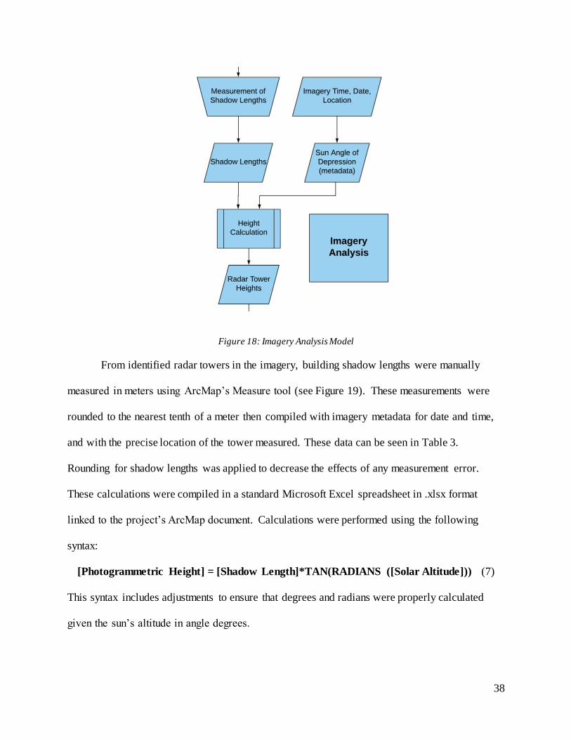
Figure 18: Imagery Analysis Model
From identified radar towers in the imagery, building shadow lengths were manually
measured in meters using ArcMap’s Measure tool (see Figure 19). These measurements were
rounded to the nearest tenth of a meter then compiled with imagery metadata for date and time,
and with the precise location of the tower measured. These data can be seen in Table 3.
Rounding for shadow lengths was applied to decrease the effects of any measurement error.
These calculations were compiled in a standard Microsoft Excel spreadsheet in .xlsx format
linked to the project’s ArcMap document. Calculations were performed using the following
syntax:
[Photogrammetric Height] = [Shadow Length]*TAN(RADIANS ([Solar Altitude])) (7)
This syntax includes adjustments to ensure that degrees and radians were properly calculated
given the sun’s altitude in angle degrees.
Page 51
39
Figure 19: Example Shadow Measurement in Multispectral Imagery. Satellite image(s) courtesy of the DigitalGlobe
Foundation.
To accurately measure the height of radar towers, the height from the base of the tower
on land above sea level was additionally measured and added to the overall height. Rather than
create a formal elevation model, this study estimated the altitude of island surfaces based on tide
changes in the region. Assuming the surfaces of pre-planned, man-made islands were at least one
meter above the maximum tide in the region, one meter was added to the highest diurnal high
tide mark for the Spratly chain for the month of imagery capture, at 0.6 m, for a total of 1.6 m
added (Brainware n.d.). This value estimates tide heights based on sensor data throughout the
region, which share tidal rhythms (Yanagi et al. 1997). Likewise, while the exact location of the
Page 52
40
radar sensor within the domed cover atop each structure is unknown, this study assumes the
highest possible point possible.
Table 3: Tower Height Measurements and Height Calculations
Tower
ID
Shadow
Length
Sun Altitude
Angle
Photogrammetric Height
(m) Absolute Height (m)
01 34.8 51.7 44.06 45.66
02 25.4 51.7 32.16 33.76
03 21.4 51.7 27.10 28.70
04 20.6 51.7 26.08 27.68
05 30.4 51.7 38.49 40.09
10 23.1 53.6 31.33 32.93
11 24.9 53.6 33.77 35.37
12 21.7 53.6 29.43 31.03
13 21.3 53.6 28.89 30.49
21 28.8 50.7 35.19 36.79
22 25.8 50.7 31.52 33.12
23 22.2 50.7 27.12 28.72
24 23.1 50.7 28.22 29.82
3.2.3. Buffer Creation
These heights formed the core data set for radar range analysis as discussed in Chapter 2.
The first step to confirming radar ranges was to calculate ranges for various altitudes using
Equation 3 and 4. For geospatial analysis, these ranges and other data were converted to buffers
based on range and location of origin as displayed by Figure 20.
Page 53
41
Figure 20: Buffer Creation Model
To calculate appropriate radar horizon ranges (or radar LOS) Equation 4 was used in the
previously mentioned linked Excel table. To yield results in meters, the calculation was adjusted
to the following final syntax:
[Range] = 4.12*((SQRT([Absolute Height])+SQRT([Investigated Altitude])))*1000 (8)
where the Investigated Altitude was adjusted to 0; 3,000; and 10,000 respective of Surface, Mid,
and High Altitudes. The reciprocal equation (Equation 5) was subsequently used to reverse
CSIS/AMTI assumed ranges in the following syntax, which was used to calculate both minimum
tower heights for a given altitude and range, and to calculate minimum visible altitude for a
given tower height and range:
[Unknown Height] = (([Range]/4.12)-(SQRT([Known Height])))^2 (9)
Using locations specific to each radar tower, buffers were created based on respective
tower height for Surface (0 m), Mid Altitude (3,000 m), and High Altitude (10,000 m) ranges,
seen in Table 4. Additionally, other weapon system data was used to create buffers based on
island centroid locations, using ranges as previously discussed in Table 1.
Page 54
42
Buffers were created using the Buffer (Analysis) tool in ArcGIS, selecting field values
for buffer distance, thus creating a unique buffer for each tower depending on its unique radar
horizon (see Figure 21). This process was repeated for each altitude (“Surface” at 0 m, “Mid
Altitude” at 3,000 m, and “High Altitude” at 10,000 m) creating 39 unique buffers in three
shapefiles. These undissolved buffers were created primarily for visualization.
Table 4: Radar Horizon Ranges at Various Altitudes
Tower
ID
Range at Surface Altitude
(km)
Range at 3,000m Altitude
(km)
Range at 10,000m Altitude
(km)
01 27.84 253.50 439.84
02 23.94 249.60 435.94
03 22.07 247.73 434.07
04 21.68 247.34 433.67
05 26.09 251.75 438.09
10 23.64 249.30 435.64
11 24.50 250.17 436.50
12 22.95 248.61 434.95
13 22.75 248.41 434.75
21 24.99 250.65 436.99
22 23.71 249.37 435.71
23 22.08 247.74 434.08
24 22.50 248.16 434.50
Page 55
43
Figure 21: Buffer Selections
Further buffers were created to compare area coverage between varying radar horizon
estimations and calculation methods. These dissolved buffers consisted of a single polygon
whose area could be measured for the collective of all towers. This area data was extracted from
the automatically generated attribute table.
3.2.4. Combined Analysis
These buffers were then overlaid for a combined analysis (modeled in Figure 22). An
average distance between each of the island’s centroids was measured using the Point Distance
Tool, which averaged to 234,014.4 m from one island centroid to the another.
Page 56
44
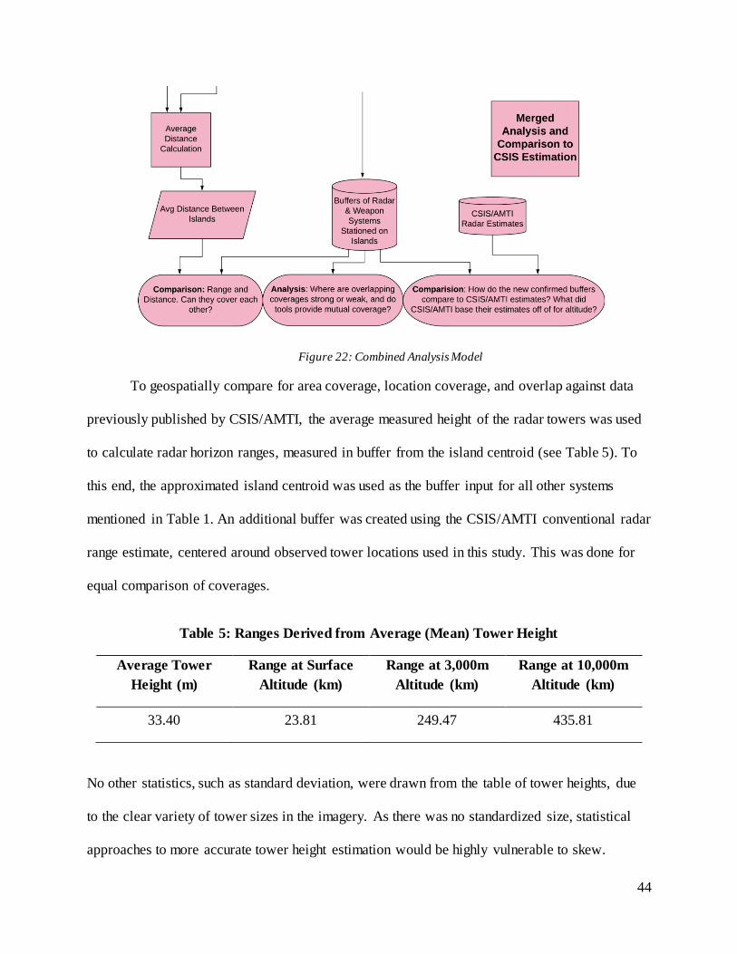
Figure 22: Combined Analysis Model
To geospatially compare for area coverage, location coverage, and overlap against data
previously published by CSIS/AMTI, the average measured height of the radar towers was used
to calculate radar horizon ranges, measured in buffer from the island centroid (see Table 5). To
this end, the approximated island centroid was used as the buffer input for all other systems
mentioned in Table 1. An additional buffer was created using the CSIS/AMTI conventional radar
range estimate, centered around observed tower locations used in this study. This was done for
equal comparison of coverages.
Table 5: Ranges Derived from Average (Mean) Tower Height
Average Tower
Height (m)
Range at Surface
Altitude (km)
Range at 3,000m
Altitude (km)
Range at 10,000m
Altitude (km)
33.40 23.81 249.47 435.81
No other statistics, such as standard deviation, were drawn from the table of tower heights, due
to the clear variety of tower sizes in the imagery. As there was no standardized size, statistical
approaches to more accurate tower height estimation would be highly vulnerable to skew.
Page 57
45
Chapter 4 Results
The maps and analysis in this chapter utilize data and methodologies discussed in Chapter 3 to
prove the efficacy of this thesis’s proposed model of shadow analysis for radar horizon
estimation, and for comparison of the described model’s output against previous published
estimates by CSIS/AMTI. Chapter 5, alternatively, discusses the accuracy and shortcomings of
this methodology and case study. It should be noted now, however, that much of this study relied
on manual processes including measurements and visual approximations due to the lack of
geospatial data available for such recently created features.
Overall, the methodology successfully provided necessary geospatial data to improve and
update previous radar range estimates with more precise calculations. There were noticeable
differences between this methodology’s results and those of previous estimates. Due to the
negatively exponential nature of the involved math, however, these differences converged as
scale increased.
4.1. Coverage Results
The measurement of radar horizons, based on shadow-to-height and LOS calculations
detailed in Chapter 2, resulted in calculated areas of coverage for every inspected radar tower. As
outlined in Chapter 3, tower heights were calculated using Equation 6; radar horizons were
subsequently calculated using Equation 4. All reverse analysis for unknown heights used
Equation 5. Coverages based on this project’s methodology for radar horizon calculation are
found in Figure 23. These calculations are also recorded in Table 4. Additionally, the average
tower height was used to create buffers centered from the approximated island centroids (see
Figure 11). This data, visualized in Figure 24, acts as a simpler approximation of data found in
Figure 23.
Page 58
46
Figure 23: Final Radar Horizon Calculations from Shadow Analysis Method
Page 59
47
Figure 24: Radar Horizons Calculated Using Average Tower Height and Island Centroids
Page 60
48
4.1.1. General Assessment of Coverage
The buffers of newly calculated radar horizons were additionally overlaid with buffers
created for reported A2AD weapon systems, as visualized in Figure 25 below.
Figure 25: Compiled Map of Calculated Radar Horizons & Other A2AD Weapon Systems
While almost every tool deployed on one island was covered by its own kind from a
neighboring island, this resulted in a triple coverage for all tools except the HQ-9 surface to air
Page 61
49
missile. Fiery Cross Reef and Mischief Reef islands were reliant on Subi Reef for secondary
coverage of HQ-9 anti-air defense.
4.1.2. Gap Estimation
There are clear and noticeable gaps in coverage between radar ranges. Using the averaged
tower height and averaged island distance, radar towers leave 186.4 km unmonitored surface (0
m altitude) between each island. However, this observational blind spot could be monitored by
radar coverage from unmeasured islands discussed in Chapter 1, or from OTH/HF radar, as seen
in Figures 29 and 30.
4.1.3. Horizons at Fixed Distance
Given the averaged distance between each island, the radar horizon altitude was
calculated using the average tower height via Equation 5. The resulting altitude, 2603.09 m, is
within the “Mid Altitude” boundary of 3,000 m. This indicates that on average, each island is
capable of observing all altitudes at or beyond Mid Altitude directly above each other island.
4.2. Radar & Weapon System Cooperation & Range Comparison
While radar is the first link in the A2AD “kill-chain,” and the primary focus of this study,
the tool’s interaction with other A2AD systems is vital for comparison. With shared ranges, the
tools may work together to successfully cooperate. Radar observation may aid weapon targeting
or may alert personnel and automated systems of a target’s existence in the first place. The
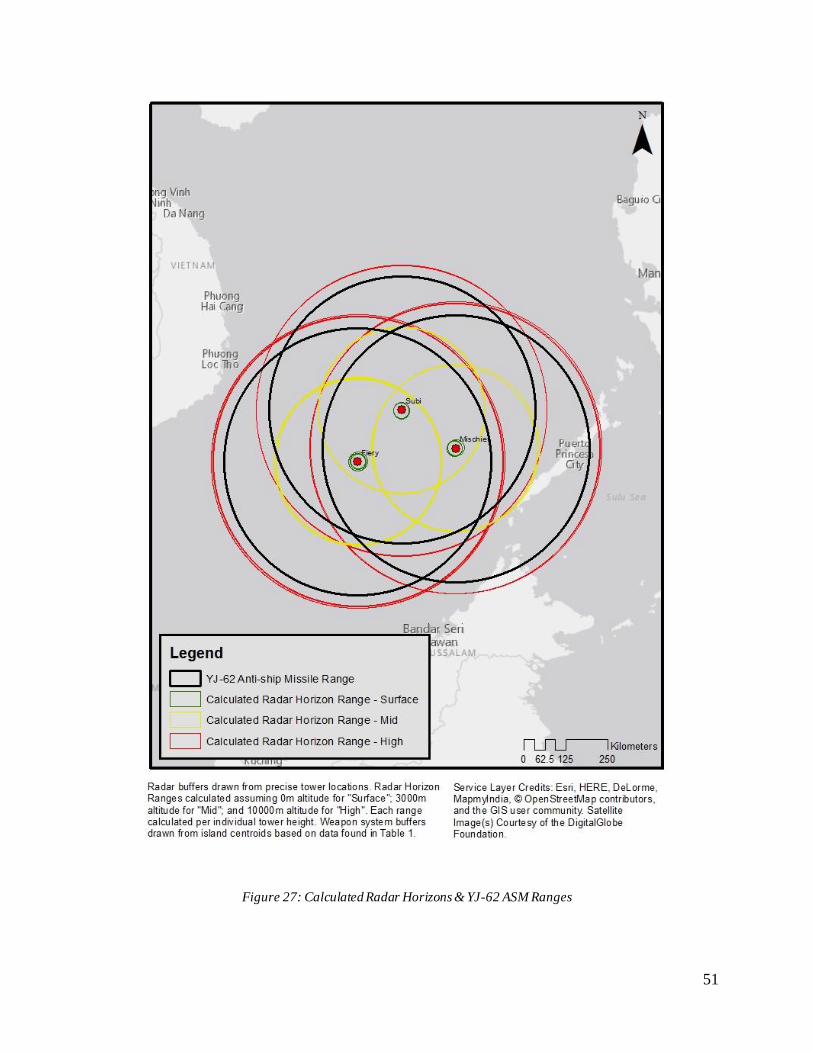
following Figures 26-29 visualize the comparative coverages of known weapon system ranges,
discussed in Table 1, with this study’s calculated radar horizons. For independent mapping of
weapon systems reported by CSIS/AMTI on Fiery Cross, Mischief, and Subi Reef, see Appendix
C.
Page 62
50
Figure 26: Calculated Radar Horizons & HQ-9 SAM Ranges
Page 63
51
Figure 27: Calculated Radar Horizons & YJ-62 ASM Ranges
Page 64
52
Figure 28: Calculated Radar Horizons & J-10 Fighter Operational Ranges
Page 65
53
Figure 29: Calculated Radar Horizons & Estimated OTH/HF Radar Ranges
Page 66
54
4.2.1. Assessment of Overlap
Calculated radar horizons exceeded HQ-9 SAM ranges at the Mid Altitude bracket,
meaning that the entirety of the HQ-9’s potential range launched from Fiery Cross, Mischief, or
Subi Reef would be within radar observation above 3,000 m altitude. Using Equation 5 and the
average tower height, the radar horizon at the HQ-9’s maximum reported range is 2504.61 m
altitude.
While the calculated radar horizons encompassed reported ranges for the YJ-62 anti-ship
missile system, conventional aerial radar is of little use for this tool. Anti-ship missiles naturally
target surface-traversing ships, rather than airships or other objects far above the surface of the
Earth. To this end, Equation 4 was used to calculate the radar horizon for a 15 m tall object, such
as an arbitrarily-heighted ship, using average tower heights. The resulting 39.7669 km distance is
well within the YJ-62’s range, leaving longer distances to targeting through OTH/HF radar or
observation by other means.
The longest-range weapon system included in this study, the J-10 Fighter Aircraft, vastly
exceeded the radar horizon ranges of radar towers measured on Fiery Cross, Mischief, and Subi
Reefs. While the unloaded range of the aircraft is reported by Kable Intelligence to be 1,850 km,
the operational, or combat, range of the aircraft was used at 550 km. At the edge of the J-10’s
operational range from one of the study’s focused islands, the radar horizon for an average height
radar tower is 16311.37 m altitude. This altitude nears the operational flight ceiling of the
aircraft.
OTH/HF radar stands as the only other observational tool included in this study. While
the maximum range reported by CSIS/AMTI is dubious due to the wide variation in ranges for
OTH/HF (see Chapter 2), the published 300 km range was compared to calculated radar horizon
ranges seen in Figure 29. Using Equation 5 and for an average height radar tower, the radar
Page 67
55
horizon at the published OTH/HF radar range is 4493.88 m altitude. Practically, outside of 300
km distance from this study’s island foci, all targets below this altitude would be unobservable
by both radar methods when measured by this study’s calculation and accepted estimates.
It should also be noted that OTH/HF range estimations created overlapping coverage of
each island by both other Big Three bases. Though only by narrow margins (see Figure 30) Fiery
Cross Reef (inset) and Mischief Reef OTH/HF exceed their separation distance and provide
coverage for one another. This indicates a preplanning of island creation, or, more likely, a
convenient choice of range estimate.
Figure 30: The Narrow Margins of OTH/HF Ranges with Fiery Cross Reef Inset
Page 68
56
4.3. Range Corrections and Calculations
This thesis attempts to calculate the true radar horizons of radar towers identified on
Fiery Cross, Mischief, and Subi Reefs in the SCS. In doing so, it provides a verifiable alternative
to provided radar horizon ranges published by CSIS/AMTI. It is a useful case study of how the
methodology discussed in Chapter 3 can be used to calculate and map radar horizons, but also of
how the methodological processes can be used to reverse engineer existing data. It is unclear
what CSIS/AMTI’s estimate is limited by: radar horizon or radar strength. Radar systems can
only detect objects if the power of the radar signal is strong enough to reach a distant target,
bounce off that target, and return. CSIS/AMTI may well assume that the strength of signal
emitted by radar systems in the SCS is only sufficient to reach their cited 50 km distance from
the structures. However, there is no evidence either way to suggest a signal strength limitation, or
lack there of. Therefore, this case study investigates CSIS/AMTI published ranges assuming no
limitation to signal strength, in an ideal situation where the only limit is the radar horizon.
4.3.1. CSIS/AMTI Assumed Tower Height
It is worthwhile to compare the potential of a tower based on published estimates versus
this study’s calculations. In their estimation, CSIS/AMTI does not report what altitude their 50
km conventional radar range corresponds to; for the sake of this section, it is assumed that the
estimate is not a limit of radar signal strength as discussed above. Therefore, a lack of announced
altitude will equate to 0 m altitude. This 0m altitude at 50 km distance is significantly lower than
the radar horizon of structures calculated in Section 4.1. Using Equation 5, the average height
tower has a radar horizon at 40.41 m altitude at this same 50 km range.
Page 69
57
4.3.2. Adjusting for CSIS/AMTI Range Estimation
It is nonetheless useful to evaluate the hypothetical implications of CSIS/AMTI’s
estimate. To determine how deviant this study’s results are from the published estimates, the
estimated range can be reverse-calculated to tell the necessary height of radar with such a radar
horizon. Utilizing Equation 5, the height of a tower capable of observing an object at 0 m altitude
within the radio spectrum at 50 km away is at minimum 147.28 m tall. This exceeds the average
tower height measured in this study by 113.88 m. While this height is not inconceivable, nor is it
uncommon for radar sensors to be placed on natural geographic features to achieve such heights,
no buildings approaching this size were evident in the imagery. For all radar horizon ranges of a
tower of this hypothetical height, see Table 6.
Table 6: Radar Horizons of CSIS/AMTI Assumed Tower Height
Minimum
Required Height
for CSIS/AMTI Est
Range at Surface
Altitude (km)
Range at 3,000 m
Altitude (km)
Range at 10,000 m
Altitude (km)
147.28 50 275.66 461.10
4.3.3. Utilizing CSIS/AMTI Assumed Tower Heights
The coverages from Table 6 were visualized and plotted in the same manner as calculated
radar horizon coverages from known precise radar tower locations (see Figure 31).
Page 70
58
Figure 31: Radar Horizons Calculated using CSIS/AMTI Assumed Tower Height
Page 71
59
4.3.4. Final Coverage Differences
It is clear that the CSIS/AMTI estimate, and the hypothetical sensor locations required for
its actualization, vary from ranges calculated by shadow-height analysis in this study. Ultimately,
this variation in coverage was visualized by altitude category in Figures 32-34. It is important to
evaluate these differences not only in distance but also area. The discrepancy in coverage
between a single tower of necessary height to meet CSIS/AMTI’s radar range estimate and that
of a single tower of average height is therefore outlined in Table 7.
Likewise, the total observable area within each altitude category’s radar horizon was
calculated using the precise tower locations identified by study for the three focused islands. This
data was derived from dissolved radar buffers, and the percent difference is reported in Table 8.
Table 7: Observable Area Differences Per Tower
Area at Surface
Altitude (km2)
Area at 3,000 m
Altitude (km2)
Area at 10,000 m
Altitude (km2)
Average Calculated Height 1781.05 195520.8 596684.3
CSIS/AMTI Assumed Height 7853.98 238727.6 670554.1
Area for Average Calculated
Height as Percentage of
CSIS/AMTI Minimum Height
23 % 82 % 89 %
Page 72
60
Figure 32: Radar Horizon Range Discrepancy between Shadow Analysis Calculations and CSIS assumed height
towers at Surface Altitude
Page 73
61
Figure 33: Radar Horizon Range Discrepancy between Shadow Analysis Calculations and CSIS assumed height
towers at Mid Altitude
Page 74
62
Figure 34: Radar Horizon Range Discrepancy between Shadow Analysis Calculations and CSIS assumed height
towers at High Altitude
Page 75
63
Table 8: Observable Area Differences From Tower Locations
Total Area at
Surface (km2)
Total Area at
3,000m (km2)
Total Area at 10,000m
(km2)
Average
Calculated Height
6503190789.80 387274251358.84 924126470728.96
CSIS/AMTI
Assumed Height
24561345968.31 446527333988.85 1012080290777.18
Total Area for
Average
Calculated Height
as Percentage of
CSIS/AMTI
Minimum Height
26 % 87 % 91%
Page 76
64
Chapter 5 Conclusions
This thesis was prepared to test the viability of using shadow photogrammetry in combination
with radar propagation equations to map radar horizon ranges. The measurement of radar
structure shadows allowed for radar horizon estimation, resulting in calculable radar ranges at
various heights, as seen throughout the provided figures in Chapter 4 and the appendices. These
measurements varied greatly from previous rule-of-thumb estimates provided by CSIS/AMTI
and suggest a potentially more limited radar range than expected.
The results of the study prove the use of shadow photogrammetry and GIS as a radar
range estimation method, giving detailed radar horizons for every radar tower. These ranges
nonetheless display ideal conditions, and rest on multiple assumptions. In this regard, the study is
limited by key factors, as well as the limited scope of this investigation. Inaccuracies originating
from the study method itself, its limited scope, and lack of data resources may be overcome in
future work.
5.1. Assessment of Methodology & Results
This study’s methodology proved successful as a trial of integrated RS, GIS, and
trigonometry as intended. The sheer volume of data provided by the DigitalGlobe Foundation – a
problem that in itself is often a geospatial scientist’s dream – proved a challenge for off-the-shelf
GIS systems, and a variety of tools were necessary to filter data to an appropriately narrow
scope. The use of mathematics and GIS data proved successful, as measurements were
effectively integrated from RS sources, moved to conventional spreadsheet tools for calculation,
and linked into a GIS for mapping and geographic calculations.
Radar horizon calculations made by this study varied substantially from CSIS/AMTI
estimates. Radar horizons for measured towers on Fiery Cross, Mischief, and Subi Reefs at
Page 77
65
average fell short of CSIS/AMTI range estimates by over 50% at surface altitude. Likewise, area
coverage of calculated radar horizons was roughly 25% of the area expected by CSIS/AMTI
estimates. Hypothetical situations in which CSIS/AMTI estimates could be made valid were
modelled and compared to this study’s calculated tower heights and radar horizons. These
hypothetical scenarios are outlined in Section 4.3, which show that the overall deviation in range
and area coverage of estimate to calculation decreased as range increased due to the negatively
exponential nature of Earth’s geometry curving away from the sensor.
The resulting radar horizon data indicates severe gaps in PRC radar coverage from
structures on Fiery Cross, Mischief, and Subi Reefs. The limited range of surface horizons
discussed in Section 4.1 allows for wide swathes of sea surface to remain out of conventional
radar observation. These unobservable locations are also potentially below the minimum range
of OTH/HF radar systems, increasing the vulnerability of these blind spots. The data suggests
that conventional radar towers measured on the islands are not tall enough to provide sufficient
coverage of the region at altitudes commensurate with other A2AD tools, as discussed in Section
4.2. Many tools’ ranges exceed the coverage distances of conventional radar structures at
appropriate altitudes. For example, while PRC anti-ship missiles may have enormous ranges,
conventional radar would be inappropriate for targeting uses at such distance. This indicates a
reliance on other targeting methods for such weapons. Likewise, the newest fighter aircraft
available to the PRC is only covered by conventional ground-based radar at altitudes
approaching its unloaded altitude ceiling (see Kable n.d.).
While there are other islands in the Spratly chain artificially created by the PRC, the three
islands circumscribed by the Fiery Cross, Mischief, and Subi Reef constructions (Johnson Reef
South, Hughes Reef, and Gavens Reefs) are not reported to house OTH/HF radar systems,
Page 78
66
airfields, or extensive conventional radar arrays at the time of writing (CSIS/AMTI). These
islands presently appear reliant on Fiery Cross, Mischief, and Subi Reef installations for many
A2AD defenses. Therefore, the defensive capabilities, including the radar horizon ranges, of the
“Big Three” reefs are vital to understanding A2AD defenses of the PRC’s Spratly construction.
The study methodology initially planned to make use of GIS data provided by
CSIS/AMTI. This could have potentially included analysis of any noted interior Spratly
construction using average tower height data gathered from Fiery Cross, Mischief, and Subi
Reefs. The poor data quality precluded this expansion.
5.2. Study Assumptions
There are multiple key assumptions made by the study which affect its scope and
relevance. Namely, the study only investigates three of seven artificial PRC islands in the Spratly
chain, though the biggest. It’s investigation of radar coverage is also confined to conventional,
ground-based radar systems, and cannot comment on the validity of OTH/HF ranges or the
supplementation of ground-based systems with signals from aircraft or other methods of aerial
surveillance. The methodology also relied greatly upon CSIS/AMTI reports for radar structure
location and other details regarding the study topic. Though this study rejects conventional radar
range estimates to create calculated radar horizons, it relies on similar estimates for other A2AD
tools when comparing potential weapon system cooperation. While these estimates are even
harder to correct, and likely impossible to calculate through a similar study, they represent a
worthy topic of research.
5.3. Study Limitations and Sources of Inaccuracy
As this research effort set out to primarily create geospatial data in a data-poor
environment, many of the geospatial and imagery inputs were of poor quality. GIS data from
Page 79
67
CSIS/AMTI lacked key information required for this study rendering it largely irrelevant, while
it could be argued that the methodology used in this study exceeded the validity of the
DigitalGlobe Foundation’s imagery GSDs. The vacuous data environment forced a methodology
built around manual measurement, creating accuracy concerns. Manual tower height
measurements, though rounded to reduce variability and establish a tighter control of
measurement outcome, as well as manual centroid approximation, formed key – albeit
questionable – data inputs.
This study, therefore, better proved the theory of its methodology rather than its exact
structure. Automation of this methodology is necessary to remove confounding human variables.
This would likely rely on an imagery classification system to find shadows, as used by Kwok
(2014), Wegner (2014), or Miao (2016) combined with machine learning technology to correctly
identify radar structures from the other, similar buildings. While this study did not need to
measure shadow segments hidden behind radar structures due to fortuitous imagery angles, this
methodology does not propose a solution to the issue. Additionally, shadows in this study were
rarely spread over rough surfaces and were assumed to be spread across even surfaces. Solutions
to these problems must be solved with image classification or inSAR as used by Wegner (2014),
and the potential referencing of more advanced math and high-resolution DEM data.
5.4. Conclusions & Future Work
This study was performed to create geospatial data where current resources were lacking.
Future research is needed to create this base data for analysis – much of this reliant upon the
scarcity of even general, unstructured information from which GIS data can be created. The
greatest takeaway from this study is the ability to create tailored geospatial data – in this case
targeted toward radar horizon range estimation – in the limited data environment of foreign
Page 80
68
defense analysis. The combination of RS, GIS, and trigonometry involved created defensible
calculations for radar horizons, and offered alternative to previous, unproven radar range
estimates. While the study relied on manual measurement and approximation, it provides a
roadmap to future study and potential automation of similar efforts.
Future research may produce a wide variety of useful intelligence on PRC A2AD
capabilities. While Chapter 2 discussed natural resources and lines of communication through
the region, air defense identification zones (ADIZ) may be more appropriate for evaluation in
conjunction with this project’s data. At what altitudes Chinese radar can enforce an ADIZ is a
potential topic of investigation. Further, the observational capabilities of OTH/HF radar and a
more thorough understanding of radar blind spots should be studied, including models and
visualizations with more direct utilization of the Z-axis.
This study’s methodology can most directly be expanded to the study of other islands in
the SCS, especially the remaining Spratly islands. To that end, the data of this project could be
made far more applicable with inclusion of radar horizon limits from these islands. Construction
on Johnson, Hughes, and Gavens Reefs may increase radar coverage within the circumscribed
“Big Three” triangle by lowering the minimum radar horizon with more proximal radar
structures, though they are not expected to greatly increase the observable area or reduce the
minimum radar horizons for locations outside the Spratlys.
Improvement to this thesis is dependent upon time and resources. In the immediate term,
this same study methodology could be applied to further sites in the SCS to calculate the radar
horizons of other towers in the region that match similar description, as discussed above. These
sites would likely come from identification in CSIS/AMTI figures, available through their web
hosting. To expand the impact of the study, a more medium-term goal could be to integrate radar
Page 81
69
horizon data from this study and any other known radar sites to examine the overlap of radar
observation and natural resources in the region, territorial claims, or ADIZ boundaries, perhaps
performing spatial analysis on the coverage dimensions between the two. To increase accuracy
of measurement while maintaining manual control, multiple images could be used to make
measurements with the results averaged. DEM data could also be added to get more accurate
evaluation of surface heights to increase the accuracy of the current 1.6 m estimation discussed
in Chapter 3. The shadow-height calculation strategy could be evaluated using ground-truthing
against objects of similar size and shape to radar towers in an environment where knowledge of
object size was available. Long-term, this study could benefit greatly from automation of
measurements and calculations. Automation strategies could be adapted from Liasis & Stavrou
(2016) or Wegner (2014), but for a data-scarce environment. Ultimately, the creation of a neural
network for radar array identification within the imagery could be used to automate the entire
methodology, with machine learning processes finding radar structures, automatically measuring
their heights, calculating radar horizons based on these heights, and creating appropriate range
buffers. This would likely look like an expansion of work by Kwok (2014) and Miao (2016) but
adapted for object-oriented identification as seen in studies by Shimoni (2011) or McGlone
(1994) and with a very different study focus. Eventually, this information could also be mapped
in three dimensions, creating models similar to those of Kostic & Rancic (2003).
Cumulatively, this project effectively provided an initial stepping stone for verifiable
radar range calculations in the SCS. This relied largely on imagery inputs, and only began the
process of creating geospatial data for future research usage. Exploration on this frontier is
necessary for a verifiable understanding of the PRC’s A2AD capabilities in the SCS, and the
fulfilment of US strategy goals.
Page 82
70
References
Adeline, K.R.M., M. Chen, X. Briottet, S.k. Pang, and N. Paparoditis. "Shadow Detection in
Very High Spatial Resolution Aerial Images: A Comparative Study." ISPRS Journal of
Photogrammetry and Remote Sensing 80 (2013): 21-38. Web.
Al-Najdawi, Nijad, Helmut E. Bez, Jyoti Singhai, and Eran.a. Edirisinghe. "A Survey of Cast
Shadow Detection Algorithms." Pattern Recognition Letters 33.6 (2012): 752-64. Web.
Alkanat, Ömer. "Determing the Surface-to-Air Missile Requirement for Western & Southern
Part of the Turkish Air Defense System”. MS Thesis (2008): n. pag. Air Force Institute of
Technology - Wright-Patterson Air Force Base, Ohio. Department of the Air Force. Air
University. Web. <http://www.dtic.mil/dtic/tr/fulltext/u2/a483275.pdf>.
AMTI. “Another Piece of the Puzzle.” Asia Maritime Transparency Initiative, Center for
Strategic and International Studies, 22 Feb. 2016, amti.csis.org/another-piece-of-the-
puzzle/.
Ashdown, Neil. “What Is China's HQ-9 Air Defense System Capable of?” Edited by Gabriel
Domínguez, DW.COM, Deutsche Welle, 17 Feb. 2016, www.dw.com/en/what-is-chinas-
hq-9-air-defense-system-capable-of/a-19053690.
Bacon, David. "Chapter 14: Terrestrial Line-of-sight Links." Propagation of Radiowaves. 3rd
ed. N.p.: IET, 2012. Http://dx.doi.org/10.1049/PBEW056E. Print
Bader, Jeffrey A. “The U.S. and China's Nine-Dash Line: Ending the Ambiguity.” Brookings,
Brookings, 28 July 2016, www.brookings.edu/opinions/the-u-s-and-chinas-nine-dash-
line-ending-the-ambiguity/.
Bell, John E., Stanley E. Griffis, William A. Cunningham, and Jon A. Eberlan. "Location
Optimization of Strategic Alert Sites for Homeland Defense." Omega 39.2 (2011): 151-
58. Web.
Booker, H.g. “Elements of Radio Meteorology: How Weather and Climate Cause Unorthodox
Radar Vision beyond the Geometrical Horizon.” Journal of the Institution of Electrical
Engineers - Part IIIA: Radiolocation, vol. 93, no. 1, 1946, pp. 69–78., doi:10.1049/ji-3a-
1.1946.0025.
Brainware, LLC. “Tide Predictions for Any Location in the World.” WorldTides, University of
Oregon, www.worldtides.info/.
Page 83
71
Brown, Peter J. "Calculated Ambiguity in the South China Sea." Asia Times Online. N.p., 8
Dec. 2009. Web.
Buszynski, Leszek. "The South China Sea: Oil, Maritime Claims, and U.S.-China Strategic
Rivalry." The Washington Quarterly 35.2 (2012): 139-56. Web.
Cheng, Dean. "The U.S. Needs an Integrated Approach to Counter China's Anti-Access/Area
Denial Strategy." The Heritage Foundation. N.p., 9 July 2014. Web. 09 Apr. 2017.
Cheng-yi Lin, “Taiwan’s South China Sea Policy,” Asian Survey, Vol. 37 (1997): 323– 324
China Power Team. "How much trade transits the South China Sea?" China Power. August 2,
2017. Updated September 12, 2017. Accessed October 22, 2017.
https://chinapower.csis.org/much-trade-transits-south-china-sea/
Cooper, Cortez. “Podcast: China’s New Spratly Island Defenses, with Michael McDevitt and
Cortez Cooper.” China’s New Spratly Island Defenses, with Michael McDevitt and
Cortez Cooper, Center for Strategic and International Studies, Jan. 2017,
soundcloud.com/csis-57169780/chinas-new-spratly-island-defenses.
Cordova, Henry. “Elevation Determination By Shadow Measurement From Vertical
Monoscopic Aerial Imagery.” Pecora 16 "Global Priorities in Land Remote Sensing", 23
Oct. 2005, www.asprs.org/a/publications/proceedings/pecora16/Cordova_H.pdf.
Cornwall, Chris, et al. “NOAA Solar Position Calculator.” Earth System Research Laboratory,
National Oceanic & Atmospheric Administration,
www.esrl.noaa.gov/gmd/grad/solcalc/azel.html.
Davin, Matthew E. "Anti-Access/Area Denial: Time To Ditch the Bumper Sticker?" Joint
Military Operations Department (2013): n. pag. Web.
EIA. "South China Sea Analysis." U.S. Energy Information Administration - EIA - Independent
Statistics and Analysis, 7 Feb. 2013. Web.
Evers, Hans-Dieter. "Reframing the South China Sea - Towards a Mediterranean Understanding
of Culture and Resources." Conceptions of Maritime Space: A Cultural Perspective on
the South China Sea (2013): n. pag. Web.
Franklin, Randolp, Clark Ray, and Shashank Mehta. Geometric Algorithms for Siting of Air
Defense Missile Batteries. Battelle, Columbus Division. Department of the Army, 1994.
n.d. Web.
Page 84
72
Gallagher, Michael G. "China's Illusory Threat to the South China Sea." International
Security 19.1 (1994): 169. Web.
Gao, Zhigao, and Bing Bing Jia. "The Nine-Dash Line in The South China Sea: History, Status,
and Implications." The American Journal of International Law 107.1 (2013): 98-124.
Web.
Gerson, Michael, and Alison Lawler Russell. "Conference Report." American Grand Strategy
& Seapower (2011): n. pag. Https://www.cna.org/. Center for Naval Analyses, 4 Aug.
2011. Web. Nov. 2011.
Gonsalves, Paul, Janet Burge, and Ben Popp. "Decision Support System for Theater Missile
Defense." Signal Processing, Sensor Fusion, and Target Recognition 5096.XII (2003): n.
pag. Web. 21 Apr. 2003.
Gormley, Dennis M, et al. “A Potent Vector: Assessing Chinese Cruise Missile Developments.”
National Defense University Press, Joint Force Quarterly 75, 30 Sept. 2014,
ndupress.ndu.edu/Media/News/News-Article-View/Article/577568/jfq-75-a-potent-
vector-assessing-chinese-cruise-missile-developments/.
Gungwu, Wang. "THE NANHAI TRADE: A Study of the Early History of Chinese Trade in
the South China Sea." Journal of the Malayan Branch of the Royal Asiatic Society (182)
31.2 (1958): 3-135. Web.
Guo, Jianhong, et al. “Removing Shadows from Google Earth Images.” International Journal
of Remote Sensing, vol. 31, no. 6, 30 Mar. 2010, pp. 1379–1389., doi:
http://dx.doi.org/10.1080/01431160903475316.
Haslett, Christopher. “Essentials of radio wave propagation”. Cambridge University Press, p.
119–120, 2008. Web.
Hayton, Bill. “China's 'Historic Rights' in the South China Sea: Made in America?” The
Diplomat, The Diplomat, 22 June 2016, thediplomat.com/2016/06/chinas-historic-rights-
in-the-south-china-sea-made-in-america/.
Hooker, R.D. "The Grand Strategy of the United States." INSS Strategic Monograph (n.d.): n.
pag. National Defense University Press, Oct. 2014. Web.
Hoyler, Marshall. "An unpersuasive argument for overcoming China's A2AD capability."
Naval War College Review, Autumn 2013, p. 135+. Academic OneFile, Accessed 22
Oct. 2017.
Page 85
73
Kable Intelligence. “J-10 (Jian 10) Vigorous Dragon Multirole Tactical Fighter.” Airforce
Technology, Kable Intelligence Limited, www.airforce-technology.com/projects/j-10/.
Kaplan, Robert D. "Chapter 2: China's Caribbean." Asia's Cauldron: The South China Sea and
the End of a Stable Pacific. N.p.: Random House USA, 2015. N. pag. Print.
Kostic, A., and D. Rancic. "Radar Coverage Analysis in Virtual GIS Environment." 6th
International Conference on Telecommunications in Modern Satellite, Cable and
Broadcasting Service, 2003. TELSIKS 2003. (n.d.): n. pag. Web.
Krepinevich, Andrew, Barry Watts, and Robert Work. Meeting the Anti-Access and Area-
Denial Challenge. Publication. Washington, D.C.: Center for Strategic and Budgetary
Assessments, 2003. Csbaonline.org. Web.
Kucera, Paul A., Witold F. Krajewski, and C. Bryan Young. "Radar Beam Occultation Studies
Using GIS and DEM Technology: An Example Study of Guam." Journal of Atmospheric
and Oceanic Technology 21.7 (2004): 995-1006. Web.
Kwatra, M.H.V., and S. Dai, "Shadow Removal for Aerial Imagery by Information Theoretic
Intrinsic Image Analysis", Proc. IEEE Int'l Conf. Computational Photography, 2012
Kwok, R. “Declassified high-resolution visible imagery for Arctic sea ice investigations: An
overview,” Remote Sens. Environ., vol. 142, pp. 44–56, Feb. 2014.
Larson, R. E., R. P. Hostetler, and B. H. Edwards. 1993. Precalculus: A Graphing Approach.
D. C. Heath and Company, Lexington, MA.
Lee, Victor Robert. “South China Sea: Satellite Imagery Shows China's Buildup on Fiery Cross
Reef.” The Diplomat, The Diplomat, 16 Sept. 2015, thediplomat.com/2015/09/south-
china-sea-satellite-imagery-shows-chinas-buildup-on-fiery-cross-reef/.
Li, Jinming, and Dexia Li. "The Dotted Line on the Chinese Map of the South China Sea: A
Note." Ocean Development & International Law 34.3-4 (2003): 287-95. Web.
Li, Y., Gong, P., Sasagawa, T., 2005. “Integrated shadow removal based on photogrammetry
and image analysis.” Int. J. Rem. Sens. 26 (18), 3911–3929.
Liasis, Gregoris, and Stavros Stavrou. "Satellite Images Analysis for Shadow Detection and
Building Height Estimation." ISPRS Journal of Photogrammetry and Remote
Sensing 119 (2016): 437-50. Web.
Page 86
74
Liu, Nan, Bo Huang, and Magesh Chandramouli. "Optimal Siting of Fire Stations Using GIS
and ANT Algorithm." Journal of Computing in Civil Engineering 20.5 (2006): 361-69.
Web.
McCarthy, Christopher J. "Anti-Access/Area Denial: The Evolution of Modern
Warfare." Lucent. U.S. Naval War College, 2010. Web.
McDevitt, Mike. “Podcast: China’s New Spratly Island Defenses, with Michael McDevitt and
Cortez Cooper.” China’s New Spratly Island Defenses, with Michael McDevitt and
Cortez Cooper, Center for Strategic and International Studies, Jan. 2017,
soundcloud.com/csis-57169780/chinas-new-spratly-island-defenses.
McDougall, Walter A. "Can the United States Do Grand Strategy?" The Telegram. Foreign
Policy Research Institute, 13 Apr. 2010. Web. 09 Apr. 2017.
McGlone, J. Chris, and Jefferey A. Shufelt. “Projective and Object Space Geometry For
Monocular Building Extraction.” IEEE Conference on Computer Vision and Pattern
Recognition, 2 Mar. 1994. Carnegie-Mellon University of Pittsburgh, PA, Department of
Computer Science, http://www.dtic.mil/get-tr-doc/pdf?AD=ADA277586.
Miao, Xin, Hongjie Xie, Stephen F. Ackley, and Songfeng Zheng. "Object-Based Arctic Sea
Ice Ridge Detection From High-Spatial-Resolution Imagery." Geoscience and Remote
Sensing Letters 13.6 (2016): 787-91. Web.
Nagao, M., Matsuyama, T., Ikeda, Y., 1979. “Region extraction and shape analysis in aerial
photographs.” Comput. Graph. Image Process. 10 (3), 195–223.
Nathanson, Fred E, et al. Radar Design Principles: Signal Processing and the Environment.
2nd ed., McGraw-Hill, 1991, selasl.files.wordpress.com/2011/08/mcgraw_hill_-
_radar_design_principles.pdf.
NAVAIR. “Chp 4: Radar Horizon / Line of Sight.” Electronic Warfare and Radar Systems
Engineering Handbook, United States Naval Air Systems Command, U.S. Navy's
Weapons Division Avionics Department Electronic Warfare Division, 2013.
O'Mara, Patrick R., LCDR, USN. "History’s Role in Operational Design and Planning: How
Germany’s Failed Invasion Provides Insight into US and Chinese Perspectives on
A2AD." USMC Command and Staff College (2013): n. pag. Web.
Overcash, David M. “Through the Lens of Operational Art: Countering People's Republic of
China (PRC) Aggression in a Limited Conflict Using Innovative Ways and Cost-
Page 87
75
Effective Means to Offset PRC Anti-Access Area Denial (A2AD) Capabilities. How
Should Pacific Command's (PACOM) Theater Campaign Plan Evolve in Light of the
Center for Strategic and Budgetary Assessment's (CSBA) Recent AirSea Battle Concept
(ASBC) Proposal?” Defense Technical Information Center,
http://www.dtic.mil/dtic/tr/fulltext/u2/a535576.pdf.
Page, Jeremy. “Tribunal Rejects Beijing's Claims to South China Sea.” The Wall Street Journal,
Dow Jones & Company, 12 July 2016, www.wsj.com/articles/chinas-claim-to-most-of-
south-china-sea-has-no-legal-basis-court-says-1468315137.
PDCC - Republic of China (Taiwan). Ministry of Foreign Affairs. Public Diplomacy
Coordination Council. Statement on the South China Sea. By PDCC. N.p., 7 July 2015.
Web.
Plait, Phil. “How Far Away Is the Horizon?” Discover Magazine, 15 Jan. 2009,
blogs.discovermagazine.com/badastronomy/2009/01/15/how-far-away-is-the-
horizon/#.WiKAiEqWZPY.
Raju, P. L. N., et al. “Shadow Analysis Technique for Extraction of Building Height Using
High Resolution Satellite Single Image and Accuracy Assessment.” ISPRS - International
Archives of the Photogrammetry, Remote Sensing and Spatial Information Sciences, XL-
8, 2014, pp. 1185–1192., doi:10.5194/isprsarchives-xl-8-1185-2014.
Richardson, John. "Deconstructing A2AD." The National Interest. The Center for the National
Interest, 3 Oct. 2016. Web. 09 Apr. 2017.
Rogers, T., L. Ames, and E. Martin. "The Possibity of Extending Air-Ground UHF Voice
Communications to Distances Far Beyond the Radio Horizon." IEEE Transactions on
Communications 5.1 (1957): 106-21. Web.
Shao, Yang, Gregory N. Taff, and Stephen J. Walsh. "Shadow Detection and Building-height
Estimation Using IKONOS Data." International Journal of Remote Sensing 32.22
(2011): 6929-944. Web.
Shimoni, M., Tolt, G., Perneel, C., Ahlberg, J., 2011. “Detection of vehicles in shadow areas.”
Proc. 3rd Workshop on Hyperspectral Image and Signal Processing: Evolution in
Remote Sensing, WHISPERS, 6–9 June, Lisbon, Portugal, pp. 1–4.
Skolnik, Merrill I. "Chapter 1: An Introduction to Radar." Introduction to Radar Systems. N.p.:
McGraw-Hill, 2007. N. pag. Print.
Page 88
76
Sofaer, Abraham D. "The Philippine Law of the Sea Action against China: Relearning the
Limits of International Adjudication." Chinese Journal of International Law (2016): n.
pag. Web.
Souza, George Bryan. The Survival of Empire: Portuguese Trade and Society in China and the
South China Sea, 1630-1754. N.p.: Cambridge UP, 2004. Print.
Straitiff, Stephanie L., and Robert G. Cromley. "Using GIS and K = 3 Central Place Lattices for
Efficient Solutions to the Location Set-Covering Problem in a Bounded
Plane." Transactions in GIS 14.3 (2010): 331-49. Wiley Online Library. Web.
Tsuruoka, Doug. “Undersea Cables the Achilles' Heel in Lead-up to New Cold War.” Asia
Times. NCIS Counter Intelligence Newletter, 6 Jan. 2018,
www.atimes.com/article/undersea-cables-achilles-heel-lead-new-cold-war/.
Valtr, Pavel, and Pavel Pechac. "The Influence of Horizontally Variable Refractive Index
Height Profile on Radio Horizon Range." Antennas & Wireless Propagation Letters 4
(2005): 489-91. Web.
Wang, Kuan-Hsiung. "The ROC's Maritime Claims and Practices with Special Reference to the
South China Sea." Ocean Development & International Law 41.3 (2010): 237-52. Web.
Wegner, Jan Dirk, Jens R. Ziehn, and Uwe Soergel. "Combining High-Resolution Optical and
InSAR Features for Height Estimation of Buildings With Flat Roofs." IEEE Transactions
on Geoscience and Remote Sensing 52.9 (2014): 5840-854. Web
Yanagi, Tetsuo, et al. “Co-Tidal and Co-Range Charts in the South China Sea Derived from
Satellite Altimetry Data.” La Mer, Societe Franco-Japonaise D'Oceanographie, vol. 35,
1997, pp. 85–93., www.sfjo-lamer.org/la_mer/35-3/35-3-1.pdf.
Zemmari, Reda, Martina Daun, and Ulrich Nickel. "Maritime Surveillance Using GSM Passive
Radar." 19th International Radar Symposium (2012): n. pag. Web.
Zhao, Guocai. “Analysis of the Sovereign Dispute over the Spratlys under the Present Law of
Sea”, Asian Review, Vol. 9, (Hong Kong, 1999): 22
Page 89
77
Appendix A: Data Notes
Relevant Imagery Metadata
Mischief Reef
Source: WV04 2017-12-27
Image ID: 9929b355-14fa-42e7-8408-41338ef178d9-inv
Image Clouds: 5.9%
Image Nadir: 16.3°
Bands: 4-BANDS
Max GSD (panchromatic; multispectral): 0.33m; 1.24m
Sun Elevation: 50.7°
Max Target Azimuth: 97.3°
Fiery Cross Reef
Source: GE01 2018-01-01
Image ID: 105001000D959600
Image Clouds: 18.0%
Image Nadir: 26.7°
Bands: 4-BANDS
Max GSD (panchromatic; multispectral): 0.51m; 1.84m
Sun Elevation: 51.7°
Max Target Azimuth: 35.3
Subi Reef
Source: WV03 2017-12-07
Image ID: 10400100355E1900
Image Clouds: 13.0%
Image Nadir: 21.6°
Bands: 8-BANDS
Max GSD (panchromatic; multispectral): 0.35m; 1.24m
Sun Elevation: 53.6°
Max Target Azimuth: 220.6
Manually Created Approximate Visual Centroid Locations
Island Center Lat (m) Long (m)
Mischief 12,861,812.43 1,107,671.14
Subi 12,700,467.05 1,223,722.42
Fiery Cross 12,566,668.92 1,067,786.09
Page 90
78
Appendix B: Labelled Imagery of Identified Radar Zones
Page 97
85
Appendix C: Weapon System Ranges
Page 101
89
Appendix D: Equations & Syntaxes
Equation 1
𝐷ℎ ≈ √2 ∙ 𝑅 ∙ 𝐻
Equation 2
𝐷ℎ ≈ 3.57 ∙ √𝐻
Equation 3
𝐷ℎ ≈ 4.12 ∙ √𝐻
Equation 4
𝐷𝑚𝑎𝑥 ≈ 4.12 ∙ (√𝐻𝑂𝑟𝑖𝑔𝑖𝑛 + √𝐻𝑇𝑎𝑟𝑔𝑒𝑡)
Equation 5
𝐻𝑈𝑛𝑘𝑛𝑜𝑤𝑛 ≈ (𝐷𝑚𝑎𝑥
4.12− √𝐻𝐾𝑛𝑜𝑤𝑛 )
2
Equation 6
𝑥 tan 𝜃 = ℎ
Syntax 7
[Photogrammetric Height] = [Shadow Length]*TAN(RADIANS ([Solar Altitude]))
Syntax 8
[Range] = 4.12*((SQRT([Absolute Height])+SQRT([Investigated Altitude])))*1000
Syntax 9
[Unknown Height] = (([Range]/4.12)-(SQRT([Known Height])))^2