192
Copyright by Abhishek Kumar 2010

Copyright
by
Abhishek Kumar
2010

The Thesis Committee for Abhishek Kumar
Certifies that this is the approved version of the following thesis:
Quantitative Geometric Model of Connected Carbonaceous Material in
Mudrocks
APPROVED BY
SUPERVISING COMMITTEE:
Steven L. Bryant
Jon T. Holder
Supervisor:

Quantitative Geometric Model of Connected Carbonaceous Material in
Mudrocks
by
Abhishek Kumar, B.Tech.
Thesis
Presented to the Faculty of the Graduate School of
The University of Texas at Austin
in Partial Fulfillment
of the Requirements
for the Degree of
Master of Science in Engineering
The University of Texas at Austin
December 2010

Dedication
This thesis is dedicated to my mentors, parents and friends.

v
Acknowledgements
I would like to thank my supervisor Dr. Steven L. Bryant for his support,
patience and encouragement throughout this research. Thanks to geoscientists of Bureau
of Economic Geology for providing useful comments in my thesis. I am thankful to Dr.
Jon T. Holder for reading this thesis and adding valuable comments.
I express my gratitude to the faculty and staff of the Petroleum and Geosystems
Engineering Department. And last, but not the least, I would like to thank my friends and
fellow graduate students at The University of at Texas who made my time at Austin even
more enjoyable.
I acknowledge the financial support of ExxonMobil for this research.
December 3rd, 2010

vi
Abstract
Quantitative Geometric Model of Connected Carbonaceous Material in
Mudrocks
Abhishek Kumar, M.S.E
The University of Texas at Austin, 2010
Supervisor: Steven L. Bryant
Unconventional gas resources have become important as an environment-
friendly source of fuel. It is important to understand the pore level geometries of grains
and voids in mudrocks in order to understand the flow potential of gas from these rocks.
Recent observations of nanopores within carbonaceous material in mudrocks have
led to the hypothesis that such material provides conduits for gas migration within the
mudrock matrix. This hypothesis requires that the carbonaceous material exist not as
isolated grains but as connected clusters of grains within the mudrock. To examine this
hypothesis, we develop an algorithm for the grain-scale modeling of the spatial
distribution of grains of carbonaceous matter in a matrix of non-carbonaceous material
(silt, clay). The algorithm produces a grain-scale model of the sediment which is

vii
precursor to a mudrock, then a sequence of models of the grain arrangement as burial
compacts the sediment into mudrock.
The carbonaceous material is approximated by the simplest possible geometric
model of spherical grains. These grains are distributed randomly within a population of
other spheres that represent silt and clay grains. A cooperative rearrangement algorithm is
used to generate a disordered packing of the grain mixture having a prescribed initial
porosity. This model represents the sediment precursor of the shale in its original
depositional setting. Periodic boundary conditions are imposed on the packing to
eliminate wall-induced artifacts in the grain arrangement; in effect the packing extends
infinitely in all three coordinate directions. We simulate compaction of the model
sediment by incrementally rescaling the vertical coordinate axis, repeating the
cooperative rearrangement calculation with periodic boundaries after each increment.
We determine the size distribution of clusters of touching carbonaceous grains,
focusing particularly upon the approach toward percolation (when a cluster spans the
entire packing). The model allows estimation of threshold fraction of carbonaceous
material for significantly connected clusters to form. Beyond a threshold degree of
compaction, connected clusters become much more prevalent. Other factors affecting the
threshold fraction such as ductility of the carbonaceous material is also evaluated.
Ductility is modeled by taking a grain consisting inner rigid core covered by the outer
soft shell which can be penetrated and deformed during geometrical transformation.
The emergence of large numbers of clusters, or of a few large clusters, increases
the probability that nanoporous conduits within the clusters would intersect a fracture in

viii
the mudrock. This should correlate with greater producibility of gas from the mudrock.
Thus the dependence of the statistics of the clusters upon other parameters, such as the
fraction of carbonaceous material, porosity, degree of compaction, etc., could be useful
for estimating resource quality. For example, it is observed that the threshold
concentration of carbonaceous material in the initial sediments for “significant
clustering” enough to approach percolation is about 20 percent of the volume fraction.
The degree of compaction needed to get “significant clustering” is 50%.

ix
Table of Contents
List of Tables ......................................................................................................... xi
List of Figures ...................................................................................................... xix
Chapter 1: Overview ................................................................................................1
1.1 Problem statement .....................................................................................1
1.2 Pore System and Transport Mechanism in Mudrocks ..............................1
1.3 Previous Work on Modeling Gas Transport in Shale .............................3
1.4 Organization of thesis .............................................................................6
Chapter 2: Methods for modeling the sediments .....................................................7
2.1 Introduction ...............................................................................................7
2.2 Cooperative rearrangement algorithm ......................................................7
2.3 Algorithm for simulating compaction ...................................................10
2.4 Rescaling in the direction of compaction ................................................13
2.5 Rescaling in the direction of compaction without cooperative rearrangement
..............................................................................................................14
2.6 Rescaling in the direction of compaction with cooperative rearrangement
……………………………………………………………………… 14
2.7 Cluster formation ...................................................................................16
Chapter 3: Effect of volume fraction of carbonaceous material on number of clusters
in model sediments .......................................................................................21
3.1 Algorithm for creating packings with prescribed volume fraction of grains
..............................................................................................................21
3.2 Carbonaceous material only (one component sphere packing) ..............25
3.3 Carbonaceous material with matrix (two component sphere packing)
…………................................................................................................29
3.4 Cluster length Analysis ...........................................................................35
3.5 Geometrical Transformation ...................................................................37
3.6 Aspect Ratio ............................................................................................39

x
3.7 Inherent clustering of spheres induced by cooperative rearrangement
algorithm ..............................................................................................46
Chapter 4: Effect of compaction on clustering of carbonaceous material .............53
4.1 Rescaling in the direction of compaction without cooperative
rearrangement: application to one component packings ......................54
4.2 Rescaling in the direction of compaction without cooperative
rearrangement : application to two component packings ..................58
4.3 Rescaling in the direction of compaction with cooperative rearrangement:
application to two component packings ...............................................62
4.3.1 Rigid carbonaceous material and silt/clay grains .................................63
4.3.2 Both carbonaceous and silt/clay grains are ductile ..............................69
4.3.3 Carbonaceous material is ductile and silt/clay grains are rigid ............88
4.4 Relationship of cluster statistics to porosity .........................................107
4.5 Discussion of clustering trends .............................................................111
Chapter 5: Conclusions and Future directions .....................................................113
5.1 Conclusions ...........................................................................................113
5.2 Future directions .................................................................................114
Appendix ..............................................................................................................116
Example1 .............................................................................................................146
All grains are rigid – one component sphere packing.................................146
Example2 .............................................................................................................154
All grains are ductile- two component sphere packing ...............................154
Example 3 ............................................................................................................158
Only carbonaceous grains are ductile- two component sphere packing .....158
Bibliography ........................................................................................................161
Vita… ...................................................................................................................162

xi
List of Tables
Table: 3.1 One component sphere packing representing carbonaceous material used
for analysis with prescribed solid volume representing carbonaceous
material .............................................................................................25
Table: 3.2 Normalized maximum cluster size for various volume fraction of
carbonaceous material for 100 spheres for D=0.001R ......................26
Table: 3.3 Normalized maximum cluster size for various volume fraction of
carbonaceous material for 500 spheres for D=0.001R ......................26
Table: 3.4 Normalized maximum cluster size for various volume fraction of
carbonaceous material for 1000 spheres for D=0.001R ....................26
Table: 3.5 Normalized maximum cluster size for various volume fraction of
carbonaceous material for 2500 spheres for D=0.001R ....................27
Table: 3.6 Normalized maximum cluster size for various volume fraction of
carbonaceous material for 3000 spheres for D=0.001R ....................27
Table: 3.7 Normalized maximum cluster size for various volume fraction of
carbonaceous material for 3500 spheres for D=0.001R ....................27
Table: 3.8 Normalized maximum cluster size for various volume fraction of
carbonaceous material for 5000 spheres for D=0.001R ....................28
Table: 3.9 Composition of two component packings: Carbonaceous material with
other grains for target porosity of 70%; the desired number of
carbonaceous material spheres is 1000. Volume fraction refers sediment
bulk volume ......................................................................................30

xii
Table: 3.10 Composition of two component packings: Carbonaceous material with
other grains for target porosity of 60%; the desired number of
carbonaceous material spheres is 1000. Volume fraction refers sediment
bulk volume ......................................................................................31
Table: 3.11 Composition of two component packings: Carbonaceous material with
other grains for target porosity of 50%; the desired number of
carbonaceous material spheres is 1000. Volume fraction refers sediment
bulk volume ......................................................................................31
Table 3.12: Cluster length and cluster aspect ratios for D=0.001R and 5 percent
carbonaceous material of bulk volume and 100 spheres with radius =
3.56 units for one component sphere packing after the geometrical
transformation ...................................................................................40
Table 3.13: Cluster length and cluster aspect ratios for D=0.001R and 10 percent
carbonaceous material of bulk volume and 100 spheres with radius =
4.42 units for one component sphere packing after the geometrical
transformation ...................................................................................41
Table 3.14: Cluster length and cluster aspect ratios for D=0.001R and 15 percent
carbonaceous material of bulk volume and 100 spheres with radius =
5.03 units for one component sphere packing after the geometrical
transformation ...................................................................................42
Table 3.15: Cluster length and cluster aspect ratios for D=0.001R and 20 percent
carbonaceous material of bulk volume and 100 spheres with radius =
5.52 units for one component sphere packing after the geometrical
transformation ...................................................................................43

xiii
Table 3.16: Cluster length and cluster aspect ratios for D=0.001R and 25 percent
carbonaceous material of bulk volume and 100 spheres with radius =
5.89 units for one component sphere packing after the geometrical
transformation ...................................................................................43
Table 3.17: Cluster length and cluster aspect ratios for D=0.001R and 30 percent
carbonaceous material of bulk volume and 100 spheres with radius =
6.83 units for one component sphere packing after the geometrical
transformation ...................................................................................44
Table 3.18: Maximum, minimum and average aspect ratios for one component sphere
packing of 100 spheres for D=0.001R ..............................................44
Table 4.1: Cluster frequency distribution for D=0.001R at different levels of
compaction for two component packing with 5 percent of carbonaceous
material in the initial bulk volume. Cooperative rearrangement, 1000
spheres of carbonaceous material, carbonaceous material and silt/clay
both rigid grains. ...............................................................................64
Table 4.2: Number of spheres distribution for D=0.001R at different levels of
compaction for two component packing with 5 percent of carbonaceous
material in the initial bulk volume. Cooperative rearrangement, 1000
spheres of carbonaceous material, carbonaceous material and silt/clay
both rigid grains. ...............................................................................64
Table 4.3: Cluster frequency distribution for D=0.001R at different levels of
compaction of two component packing with 10 percent of carbonaceous
material in the initial bulk volume. Cooperative rearrangement, 1000
spheres of carbonaceous material, carbonaceous material and silt/clay
both rigid grains. ...............................................................................66

xiv
Table 4.4: Number of spheres distribution for D=0.001R at different levels of
compaction of two component packing with 10 percent of carbonaceous
material in the initial bulk volume. Cooperative rearrangement, 1000
spheres of carbonaceous material, carbonaceous material and silt/clay
both rigid grains. ...............................................................................67
Table 4.5: Cluster frequency distribution for D=0.001R at different levels of
compaction of two component packing with 5 percent of carbonaceous
material in the initial bulk volume. Cooperative rearrangement, 1000
spheres of carbonaceous material, carbonaceous material and silt/clay
both ductile grains with rigid ratio =0.9R .........................................70
Table 4.6: Number of spheres distribution for D=0.001R at different levels of
compaction of two component packing with 5 percent of carbonaceous
material in the initial bulk volume. Cooperative rearrangement, 1000
spheres of carbonaceous material, carbonaceous material and silt/clay
both ductile grains with rigid ratio =0.9R .........................................71
Table 4.7: Cluster frequency distribution for D=0.001R at different levels of
compaction of two component packing with 10 percent of carbonaceous
material in the initial bulk volume. Cooperative rearrangement, 1000
spheres of carbonaceous material, carbonaceous material and silt/clay
both ductile grains with rigid ratio =0.9R .........................................74
Table 4.8: Number of spheres distribution for D=0.001R at different levels of
compaction of two component packing with 10 percent of carbonaceous
material in the initial bulk volume. Cooperative rearrangement, 1000
spheres of carbonaceous material, carbonaceous material and silt/clay
both ductile grains with rigid ratio =0.9R .........................................74

xv
Table 4.9: Cluster frequency distribution for D=0.001R at different levels of
compaction of two component packing with 5 percent of carbonaceous
material in the initial bulk volume. Cooperative rearrangement, 1000
spheres of carbonaceous material, carbonaceous material and silt/clay
both ductile grains with rigid ratio =0.8R .........................................77
Table 4.10: Number of spheres distribution for D=0.001R at different levels of
compaction of two component packing with 5 percent of carbonaceous
material in the initial bulk volume. Cooperative rearrangement, 1000
spheres of carbonaceous material, carbonaceous material and silt/clay
both ductile grains with rigid ratio =0.8R .........................................77
Table 4.11: Cluster frequency distribution for D=0.001R at different levels of
compaction of two component packing with 10 percent of carbonaceous
material in the initial bulk volume. Cooperative rearrangement, 1000
spheres of carbonaceous material, carbonaceous material and silt/clay
both ductile grains with rigid ratio =0.8R .........................................80
Table 4.12: Number of spheres distribution for D=0.001R at different levels of
compaction of two component packing with 10 percent of carbonaceous
material in the initial bulk volume. Cooperative rearrangement, 1000
spheres of carbonaceous material, carbonaceous material and silt/clay
both ductile grains with rigid ratio =0.8R .........................................80
Table 4.13: Cluster frequency distribution for D=0.001R at different levels of
compaction of two component packing with 5 percent of carbonaceous
material in the initial bulk volume. Cooperative rearrangement, 1000
spheres of carbonaceous material, carbonaceous material and silt/clay
both ductile grains with rigid ratio =0.7R .........................................83

xvi
Table 4.14: Number of spheres distribution for D=0.001R at different levels of
compaction of two component packing with 5 percent of carbonaceous
material in the initial bulk volume. Cooperative rearrangement, 1000
spheres of carbonaceous material, carbonaceous material and silt/clay
both ductile grains with rigid ratio =0.7R .........................................83
Table 4.15: Cluster frequency distribution for D=0.001R at different levels of
compaction of two component packing with 10 percent of carbonaceous
material in the initial bulk volume. Cooperative rearrangement, 1000
spheres of carbonaceous material, carbonaceous material and silt/clay
both ductile grains with rigid ratio =0.7R .........................................86
Table 4.16: Number of spheres distribution for D=0.001R at different levels of
compaction of two component packing with 10 percent of carbonaceous
material in the initial bulk volume. Cooperative rearrangement, 1000
spheres of carbonaceous material, carbonaceous material and silt/clay
both ductile grains with rigid ratio =0.7R .........................................86
Table 4.17: Cluster frequency distribution for D=0.001R at different levels of
compaction of two component packing with 5 percent of carbonaceous
material in the initial bulk volume. Cooperative rearrangement, 1000
spheres of carbonaceous material, carbonaceous material being ductile
with rigid radius ratio =0.9R and silt/clay being rigid ......................89
Table 4.18: Number of spheres distribution for D=0.001R at different levels of
compaction of two component packing with 5 percent of carbonaceous
material in the initial bulk volume. Cooperative rearrangement, 1000
spheres of carbonaceous material, carbonaceous material being ductile
with rigid radius ratio=0.9R and silt/clay being rigid .......................90

xvii
Table4.19: Cluster frequency distribution for D=0.001R at different levels of
compaction of two component packing with 10 percent of carbonaceous
material in the initial bulk volume. Cooperative rearrangement, 1000
spheres of carbonaceous material, carbonaceous material being ductile
with rigid radius ratio =0.9R and silt/clay being rigid ......................93
Table 4.20: Number of spheres distribution for D=0.001R at different levels of
compaction of two component packing with 10 percent of carbonaceous
material in the initial bulk volume. Cooperative rearrangement, 1000
spheres of carbonaceous material, carbonaceous material being ductile
with rigid radius ratio=0.9R and silt/clay being rigid .......................93
Table 4.21: Cluster frequency distribution for D=0.001R at different levels of
compaction of two component packing with 5 percent of carbonaceous
material in the initial bulk volume. Cooperative rearrangement, 1000
spheres of carbonaceous material, carbonaceous material being ductile
with rigid radius ratio =0.8 R and silt/clay being rigid .....................96
Table 4.22: Number of spheres distribution for D=0.001R at different levels of
compaction of two component packing with 5 percent of carbonaceous
material in the initial bulk volume. Cooperative rearrangement, 1000
spheres of carbonaceous material, carbonaceous material being ductile
with rigid radius ratio=0.8R and silt/clay being rigid .......................96
Table 4.23: Cluster frequency distribution for D=0.001R at different levels of
compaction of two component packing with 10 percent of carbonaceous
material in the initial bulk volume. Cooperative rearrangement, 1000
spheres of carbonaceous material, carbonaceous material being ductile
with rigid radius ratio =0.8 R and silt/clay being rigid .....................99

xviii
Table 4.24: Number of spheres distribution for D=0.001R at different levels of
compaction of two component packing with 10 percent of carbonaceous
material in the initial bulk volume. Cooperative rearrangement, 1000
spheres of carbonaceous material, carbonaceous material being ductile
with rigid radius ratio=0.8R and silt/clay being rigid .......................99
Table 4.25: Cluster frequency distribution for D=0.001R at different levels of
compaction of two component packing with 5 percent of carbonaceous
material in the initial bulk volume. Cooperative rearrangement, 1000
spheres of carbonaceous material, carbonaceous material being ductile
with rigid radius ratio =0.7 R and silt/clay being rigid ...................102
Table 4.26: Number of spheres distribution for D=0.001R at different levels of
compaction of two component packing with 5 percent of carbonaceous
material in the initial bulk volume. Cooperative rearrangement, 1000
spheres of carbonaceous material, carbonaceous material being ductile
with rigid radius ratio=0.7R and silt/clay being rigid .....................102
Table 4.27: Cluster frequency distribution for D=0.001R at different levels of
compaction of two component packing with 10 percent of carbonaceous
material in the initial bulk volume. Cooperative rearrangement, 1000
spheres of carbonaceous material, carbonaceous material being ductile
with rigid radius ratio =0.7 R and silt/clay being rigid ...................105
Table 4.28: Number of spheres distribution for D=0.001R at different levels of
compaction of two component packing with 10 percent of carbonaceous
material in the initial bulk volume. Cooperative rearrangement, 1000
spheres of carbonaceous material, carbonaceous material being ductile
with rigid radius ratio=0.7R and silt/clay being rigid .....................105

xix
List of Figures
Figure 1.1: Scanning electron micro-image of Ar-ion-beam milled surface showing
pores in organic matter (Wang and Reed, 2009) ................................2
Figure 1.2: Connected carbonaceous material in typical SEM image of shale gas
sample (Barnett shale). The connections are interpreted to have formed
as smaller, separate pieces of material come into contact during burial
and compaction. (Courtesy Dr. K Milliken, University of Texas Bureau
of Economic Geology) ........................................................................3
Figure 1.3: Schematic diagram showing high- permeability elements in gas shale:
organic matter, natural fractures, and hydraulic fractures. (Reed et al.
2009) ...................................................................................................5
Figure 2.1: Concept of periodicity as implemented in the sphere packing code. The
spheres in the unit cell are shown in the projected y-z plane in the center
of the diagram; four copies of the unit cell are placed around the center
cell. Red spheres are real spheres and green spheres are their images. A
sphere at or near one face of unit cell can thus be in virtual contact with
a sphere at or near the opposite face. Such contacts are accounted for
during the cooperative rearrangement steps. ......................................9
Figure 2.2: Schematic showing various stages of compaction. Original model
sediment is uncompacted (c=1).The final state corresponds to mudrock.
...........................................................................................................11
Figure 2.3: Schematic showing the relative motion of spheres within a box in
mechanical compaction .....................................................................13

xx
Figure 2.4: Illustration of rigid and ductile grains. For rigid grain, the rigid radius
equals grain radius R. For ductile grains, the rigid radius is less than the
grain radius R. ...................................................................................15
Figure 2.5: The criterion for touching spheres is whether the gap D between the
spheres is less than a user-specified tolerance. .................................17
Figure 2.6: Cluster size distribution for 100 spheres for one component sphere
packing for tolerance value D = 1.0 R ..............................................18
Figure 2.7: Cluster size distribution for 100 spheres for one component sphere
packing for tolerance value D = 0.1 R ..............................................18
Figure 2.8: Cluster size distribution for 100 spheres for one component sphere
packing for tolerance value D = 0.01 R ............................................19
Figure 2.9: Cluster size distribution for 100 spheres for one component sphere
packing for tolerance value D= 0.001 R ...........................................19
Figure 2.10: Cluster size distribution for 100 spheres for one component sphere
packing tolerance value D = 0.0001 R ..............................................20
Figure 2.11: Cluster size distribution for 100 spheres for one component sphere
packing for tolerance value D= 0.00001 ...........................................20
Figure 3.1: Periodic packing of 100 spheres showing 5% (left) and 10% (right) of cell
volume occupied by solid .................................................................21
Figure 3.2: Periodic packing of 1000 spheres showing 5% (left) and 10% (right) of
cell volume occupied by solid ...........................................................22
Figure 3.3: Initial point generation (Left) and particle growth (Right) in one
component sphere packing representing only carbonaceous material in
the original sediment .........................................................................23

xxi
Figure 3.4: Initial point generation (Left) and particle growth (Right) in two
component sphere packing, red colored spheres representing
carbonaceous material and green colored spheres representing silt/clay
...........................................................................................................24
Figure 3.5: Normalized maximum cluster size for D = 0.001R vs. volume fraction of
carbonaceous material for one component sphere packing ..............28
Figure 3.6: Normalized maximum cluster size for D = 0.001R vs. volume fraction of
carbonaceous material in sediment for packing of carbonaceous material
with matrix. Sediment porosity is 70 percent. Curves refer to sets of
packings in which number of carbonaceous material grains is constant
...........................................................................................................32
Figure 3.7: Normalized maximum cluster size for D = 0.001R vs. volume fraction of
carbonaceous material in sediment for packing of carbonaceous material
with matrix. Sediment porosity is 60 percent. Curves refer to sets of
packings in which number of carbonaceous material grains is constant
...........................................................................................................33
Figure 3.8: Normalized maximum cluster size for D = 0.001R vs. volume fraction of
carbonaceous material in sediment for packing of carbonaceous material
with matrix. Sediment porosity is 50 percent. Curves refer to sets of
packings in which number of carbonaceous material grains is constant
...........................................................................................................34
Figure 3.9: Cluster Length calculation in X direction ...........................................36
Figure 3.10: Selected cluster length analysis for 5 percent carbonaceous material for
one component sphere packing of 100 spheres representing
carbonaceous material with radius = 3.56 units ...............................36

xxii
Figure 3.11: Geometrical transformation for the biggest cluster from one component
sphere packing of 100 spheres representing carbonaceous material with
radius = 3.56 units .............................................................................38
Figure 3.12:Variation of LX and LY in new coordinate system showing a phase
difference of 90 degrees between them for the biggest cluster from one
component sphere packing of 100 spheres with radius = 3.56 units 39
Figure 3.13: Maximum aspect ratio of clusters vs. volume fraction of carbonaceous
material for one component sphere packing of 100 spheres for D=0.001R
...........................................................................................................45
Figure 3.13: Aspect ratio of largest cluster vs. volume fraction of carbonaceous
material for one component sphere packing of 100 spheres for D=0.001R
...........................................................................................................46
Figure 3.14: Comparison of cluster frequency vs. cluster size for D=0.001R of the
compaction stages of one component packing created by Thane‟s code
and dispersed spheres represented by suffix-2 (1000 rigid spheres of
carbonaceous material) .....................................................................48
Figure 3.15: Comparison of number of spheres vs. cluster size for D=0.001R of the
compaction stages of one component packing created by Thane`s code
and dispersed spheres represented by suffix-2 (1000 rigid spheres of
carbonaceous material) .....................................................................49
Figure 3.16: Comparison of cluster frequency vs. cluster size for D=0.001R of the
compaction stages of two component packing created by Thane`s code
and dispersed spheres represented by suffix-2 (1000 rigid spheres of
carbonaceous material and 70 % target porosity) .............................50
xxiii
Figure 3.17: Comparison of number of spheres vs. cluster size for D=0.001R of the
compaction stages of two component packing created by Thane`s code
and dispersed spheres represented by suffix-2 (1000 rigid spheres of
carbonaceous material and 70 % target porosity) .............................51
Figure 4.1: Grain packing showing the effect of compaction ................................54
Figure 4.2: Cluster frequency vs. cluster size for D =0.001R as a function of
compaction without cooperative rearrangement with 5 percent of
carbonaceous material in the initial bulk volume for one component
sphere packing (1000 spheres of carbonaceous material) .................55
Figure 4.3: Number of spheres in cluster size vs. cluster size for D=0.001R as a
function of compaction without cooperative rearrangement with 5
percent of carbonaceous material in the initial bulk volume for one
component sphere packing (1000 spheres of carbonaceous material) ..
……………………………………………………………………..56
Figure 4.4: Cluster frequency vs. cluster size for D=0.001R as a function of
compaction without cooperative rearrangement with10 percent of
carbonaceous material in the initial bulk volume for one component
sphere packing (1000 spheres of carbonaceous material) .................57
Figure 4.5: Number of spheres in cluster size vs. cluster size for D=0.001R as a
function of compaction without cooperative rearrangement with 10
percent of carbonaceous material in the initial bulk volume for one
component sphere packing (1000 spheres of carbonaceous material) ..
……………………………………………………………………..58

xxiv
Figure 4.6: Cluster frequency vs. cluster size for D=0.001R as a function of
compaction without cooperative rearrangement with 5 percent of
carbonaceous material in the initial bulk volume for two component
sphere packing (1000 spheres of carbonaceous material) .................59
Figure 4.7: Number of spheres in cluster size vs. cluster size for D=0.001R as a
function of compaction without cooperative rearrangement with 5
percent of carbonaceous material in the initial bulk volume for two
component sphere packing (1000 spheres of carbonaceous material)
...........................................................................................................60
Figure 4.8: Cluster frequency vs. cluster size for D=0.001R as a function of
compaction without cooperative rearrangement with 10 percent of
carbonaceous material in the initial bulk volume for two component
sphere packing (1000 spheres of carbonaceous material) .................61
Figure 4.9: Number of spheres in cluster size vs. cluster size for D=0.001R as a
function of compaction without cooperative rearrangement with 10
percent of carbonaceous material in the initial bulk volume for two
component sphere packing (1000 spheres of carbonaceous material)
...........................................................................................................62
Figure 4.10: Cluster frequency distribution for D=0.001R at different levels of
compaction for two component packing with 5 percent of carbonaceous
material in the initial bulk volume. Cooperative rearrangement, 1000
spheres of carbonaceous material, carbonaceous material and silt/clay
both rigid grains ................................................................................65

xxv
Figure 4.11: Number of spheres distribution for D=0.001R at different levels of
compaction for two component packing with 5 percent of carbonaceous
material in the initial bulk volume. Cooperative rearrangement, 1000
spheres of carbonaceous material, carbonaceous material and silt/clay
both rigid grains. ...............................................................................66
Figure 4.12: Cluster frequency distribution for D=0.001R at different levels of
compaction of two component packing with 10 percent of carbonaceous
material in the initial bulk volume. Cooperative rearrangement, 1000
spheres of carbonaceous material, carbonaceous material and silt/clay
both rigid grains. ...............................................................................68
Figure 4.13: Number of spheres distribution for D=0.001R at different levels of
compaction of two component packing with 10 percent of carbonaceous
material in the initial bulk volume. Cooperative rearrangement, 1000
spheres of carbonaceous material, carbonaceous material and silt/clay
both rigid grains. ...............................................................................69
Figure 4.14: Cluster frequency distribution for D=0.001R at different levels of
compaction of two component packing with 5 percent of carbonaceous
material in the initial bulk volume. Cooperative rearrangement, 1000
spheres of carbonaceous material, carbonaceous material and silt/clay
both ductile grains with rigid radius ratio =0.9R ..............................72
Figure 4.15: Number of spheres distribution for D=0.001R at different levels of
compaction of two component packing with 5 percent of carbonaceous
material in the initial bulk volume. Cooperative rearrangement, 1000
spheres of carbonaceous material, carbonaceous material and silt/clay
both ductile grains with rigid ratio=0.9R ..........................................73

xxvi
Figure 4.16: Cluster frequency distribution for D=0.001R at different levels of
compaction of two component packing with 10 percent of carbonaceous
material in the initial bulk volume. Cooperative rearrangement, 1000
spheres of carbonaceous material, carbonaceous material and silt/clay
both ductile grains with rigid radius ratio =0.9R ..............................75
Figure 4.17: Number of spheres distribution for D=0.001R at different levels of
compaction of two component packing with 10 percent of carbonaceous
material in the initial bulk volume. Cooperative rearrangement, 1000
spheres of carbonaceous material, carbonaceous material and silt/clay
both ductile grains with rigid ratio=0.9R ..........................................76
Figure 4.18: Cluster frequency distribution for D=0.001R at different levels of
compaction of two component packing with 5 percent of carbonaceous
material in the initial bulk volume. Cooperative rearrangement, 1000
spheres of carbonaceous material, carbonaceous material and silt/clay
both ductile grains with rigid radius ratio =0.8R ..............................78
Figure 4.19: Number of spheres distribution for D=0.001R at different levels of
compaction of two component packing with 5 percent of carbonaceous
material in the initial bulk volume. Cooperative rearrangement, 1000
spheres of carbonaceous material, carbonaceous material and silt/clay
both ductile grains with rigid ratio=0.8R ..........................................79
Figure 4.20: Cluster frequency distribution for D=0.001R at different levels of
compaction of two component packing with 10 percent of carbonaceous
material in the initial bulk volume. Cooperative rearrangement, 1000
spheres of carbonaceous material, carbonaceous material and silt/clay
both ductile grains with rigid radius ratio =0.8R ..............................81

xxvii
Figure 4.21: Number of spheres distribution for D=0.001R at different levels of
compaction of two component packing with 10 percent of carbonaceous
material in the initial bulk volume. Cooperative rearrangement, 1000
spheres of carbonaceous material, carbonaceous material and silt/clay
both ductile grains with rigid ratio=0.8R ..........................................82
Figure 4.22: Cluster frequency distribution for D=0.001R at different levels of
compaction of two component packing with 5 percent of carbonaceous
material in the initial bulk volume. Cooperative rearrangement, 1000
spheres of carbonaceous material, carbonaceous material and silt/clay
both ductile grains with rigid radius ratio =0.7R ..............................84
Figure 4.23: Number of spheres distribution for D=0.001R at different levels of
compaction of two component packing with 5 percent of carbonaceous
material in the initial bulk volume. Cooperative rearrangement, 1000
spheres of carbonaceous material, carbonaceous material and silt/clay
both ductile grains with rigid ratio=0.7R ..........................................85
Figure 4.24: Cluster frequency distribution for D=0.001R at different levels of
compaction of two component packing with 10 percent of carbonaceous
material in the initial bulk volume. Cooperative rearrangement, 1000
spheres of carbonaceous material, carbonaceous material and silt/clay
both ductile grains with rigid radius ratio =0.7R ..............................87
Figure 4.25: Number of spheres distribution for D=0.001R at different levels of
compaction of two component packing with 10 percent of carbonaceous
material in the initial bulk volume. Cooperative rearrangement, 1000
spheres of carbonaceous material, carbonaceous material and silt/clay
both ductile grains with rigid ratio=0.7R ..........................................88

xxviii
Figure 4.26: Cluster frequency distribution for D=0.001R at different levels of
compaction of two component packing with 5 percent of carbonaceous
material in the initial bulk volume. Cooperative rearrangement, 1000
spheres of carbonaceous material, carbonaceous material being ductile
with rigid radius ratio=0.9R and silt/clay being rigid .......................91
Figure 4.27: Number of spheres distribution for D=0.001R at different levels of
compaction of two component packing with 5 percent of carbonaceous
material in the initial bulk volume. Cooperative rearrangement, 1000
spheres of carbonaceous material, carbonaceous material being ductile
with rigid radius ratio =0.9R and silt/clay being rigid ......................92
Figure 4.28: Cluster frequency distribution for D=0.001R at different levels of
compaction of two component packing with 10 percent of carbonaceous
material in the initial bulk volume. Cooperative rearrangement, 1000
spheres of carbonaceous material, carbonaceous material being ductile
with rigid radius ratio=0.9R and silt/clay being rigid .......................94
Figure 4.29: Number of spheres distribution for D=0.001R at different levels of
compaction of two component packing with 10 percent of carbonaceous
material in the initial bulk volume. Cooperative rearrangement, 1000
spheres of carbonaceous material, carbonaceous material being ductile
with rigid radius ratio =0.9R and silt/clay being rigid ......................95
Figure 4.30: Cluster frequency distribution for D=0.001R at different levels of
compaction of two component packing with 5 percent of carbonaceous
material in the initial bulk volume. Cooperative rearrangement, 1000
spheres of carbonaceous material, carbonaceous material being ductile
with rigid radius ratio=0.8R and silt/clay being rigid .......................97

xxix
Figure 4.31: Number of spheres distribution for D=0.001R at different levels of
compaction of two component packing with 5 percent of carbonaceous
material in the initial bulk volume. Cooperative rearrangement, 1000
spheres of carbonaceous material, carbonaceous material being ductile
with rigid radius ratio =0.8R and silt/clay being rigid ......................98
Figure 4.32: Cluster frequency distribution for D=0.001R at different levels of
compaction of two component packing with 10 percent of carbonaceous
material in the initial bulk volume. Cooperative rearrangement, 1000
spheres of carbonaceous material, carbonaceous material being ductile
with rigid radius ratio=0.8R and silt/clay being rigid .....................100
Figure 4.33: Number of spheres distribution for D=0.001R at different levels of
compaction of two component packing with 10 percent of carbonaceous
material in the initial bulk volume. Cooperative rearrangement, 1000
spheres of carbonaceous material, carbonaceous material being ductile
with rigid radius ratio =0.8R and silt/clay being rigid ....................101
Figure 4.34: Cluster frequency distribution for D=0.001R at different levels of
compaction of two component packing with 5 percent of carbonaceous
material in the initial bulk volume. Cooperative rearrangement, 1000
spheres of carbonaceous material, carbonaceous material being ductile
with rigid radius ratio=0.7R and silt/clay being rigid .....................103
Figure 4.35: Number of spheres distribution for D=0.001R at different levels of
compaction of two component packing with 5 percent of carbonaceous
material in the initial bulk volume. Cooperative rearrangement, 1000
spheres of carbonaceous material, carbonaceous material being ductile
with rigid radius ratio =0.7R and silt/clay being rigid ....................104

xxx
Figure 4.36: Cluster frequency distribution for D=0.001R at different levels of
compaction of two component packing with 10 percent of carbonaceous
material in the initial bulk volume. Cooperative rearrangement, 1000
spheres of carbonaceous material, carbonaceous material being ductile
with rigid radius ratio=0.7R and silt/clay being rigid .....................106
Figure 4.37: Number of spheres distribution for D=0.001R at different levels of
compaction of two component packing with 10 percent of carbonaceous
material in the initial bulk volume. Cooperative rearrangement, 1000
spheres of carbonaceous material, carbonaceous material being ductile
with rigid radius ratio =0.7R and silt/clay being rigid ....................107
Figure 4.38: Relationship between number of clusters and sediment porosity with 5
percent of carbonaceous material in the initial bulk volume for initial
sediment porosity of 70%. Values taken from Table 4.1, Table 4.5,
Table 4.9, Table 4.13, Table 4.17, Table 4.21, Table 4.25 .............108
Figure 4.39: Relationship between number of spheres in cluster size and sediment
porosity with 5 percent of carbonaceous material in the initial bulk
volume for initial porosity 70%.Values taken from Table 4.2, Table 4.6,
Table 4.10, Table 4.14, Table 4.18, Table 4.22, Table 4.26 ...........109
Figure 4.40: Relationship between number of clusters and sediment porosity with 10
percent of carbonaceous material in the initial bulk volume for initial
porosity of 70%.Values taken from Table 4.3, Table 4.7, Table 4.11,
Table 4.15, Table 4.19, Table 4.23, Table 4.27 ..............................110
xxxi
Figure 4.41: Relationship between number of spheres in cluster size and sediment
porosity with 10 percent of carbonaceous material in the initial bulk
volume for initial porosity of 70%.Values taken from Table 4.4, Table
4.8, Table 4.12, Table 4.16, Table 4.20, Table 4.24, Table 4.28 ....111
Figure 5.1: Schematic diagram showing the roadmap of taking grain packing forward
to commercial simulator for studying multiphase effect on gas phase
permeability in mudrocks. ..............................................................115

1
Chapter 1: Overview
This Chapter gives an overview of the topics discussed in the thesis. The research
is focused on grain-scale modeling of the unconventional reservoirs in mudrocks.
1.1 PROBLEM STATEMENT
Shale gas is one of the most important unconventional gas resources. It is
increasingly becoming one of the most important energy sources for the world. Most of
the shale gas reservoirs are explored in the United States and are exploited to meet the
ever increasing demand of energy. It is important to understand the pore level geometries
of grains and voids of the mudrocks which play an important role in the transport of
hydrocarbons through them. The present work consists of making mechanistic models of
certain aspects of the evolution of mudrocks. The models focus on the effect of
mechanical compaction on the connectivity of carbonaceous material at the grain scale.
The hypothesis is that the extent to which particles of organic matter touch each other
determines the extent to which nanopores, which subsequently evolve within these
particles, could be connected within the mudrock. Greater connectivity of nanopores
should correlate with greater producibility once the mudrock has been stimulated.
1.2 PORE SYSTEM AND TRANSPORT MECHANISM IN MUDROCKS
The pore systems in mudrocks are generally composed of two types of
pores:-
a) Intergranular Pores
b) Intragranular Pores

2
The former type of pores is not common in mudrocks, and the intragranular pore
system is assumed to be the main network for storage and transport of the hydrocarbon
throughout this study. Nanopores in carbonaceous material in gas-producing mudrocks,
Figure 1.1, are attributed to thermal maturation and conversion of solid carbonaceous
matter into a fluid hydrocarbon phase. Thermal cooking of this solid carbonaceous
material results in increase of pressure within this material, resulting in the formation of
nanopores. This leads to the hypothesis that carbonaceous material particles are the
preferred conduits of hydrocarbon in mudrocks. The greater the extent to which
carbonaceous particles are connected, Figure 1.2, the greater the conductivity of these
conduits. The pore networks present in other lithofacies are generally small and isolated.
As a limiting case, we assume that these other networks do not contribute to the flow of
hydrocarbon in these types of unconventional reservoirs.
Figure 1.1: Scanning electron micro-image of Ar-ion-beam milled surface showing pores
in organic matter (Wang and Reed, 2009)

3
Figure 1.2: Connected carbonaceous material in typical SEM image of shale gas sample
(Barnett shale). The connections are interpreted to have formed as smaller,
separate pieces of material come into contact during burial and compaction.
(Courtesy Dr. K Milliken, University of Texas Bureau of Economic
Geology)
1.3 PREVIOUS WORK ON MODELING GAS TRANSPORT IN SHALE
Javadpour (2009) observed that the gas production from mudrocks was greater
than that anticipated from their Darcy permeability. Using images of nanopores obtained
by Atomic Force Microscopy, he concluded that the gas flow in nanopores cannot be
described simply by Darcy‟s equation. Taking into account of Knudsen diffusion and slip
flow he introduced an apparent permeability concept which is significant for the pore
sizes smaller than 100 nm.
The mass balance equation can be written as follows :-
2. : 0c
U c D c ct
………………………….. (1)

4
The first term in Equation 1 is the accumulation term, the second one is advection,
the third one is Knudsen diffusion and the last term is for desorption of fluid from the
surface of carbonaceous material. The parameter is the desorption constant, D is the
Knudsen diffusion and U is the advective velocity. Knudsen diffusion is an important gas
transport process in nanopores which are present in the carbonaceous material of the
mudrock system and thus relevant to the hypothesis of this study.
Roy et al. (2003) proposed a model to predict the flow characteristics for
reasonably high Knudsen number flow regimes through micro channels and nanopores.
The Knudsen number ( Kn ) is defined as the ratio of the fluid mean-free path (λ) to the
macroscopic length scale of the physical system ( ) :-
Kn
………………………………………………….. (2)
where 16 / 5 2 RT ; = viscosity; T = temperature; /Λx
and
is fluid density ; R is the universal gas constant and x is the direction of the pressure
gradient. They developed a two dimensional microscale flow model to predict the overall
flow characteristics for reasonably high Knudsen number flow in microchannels and
nanopores. If connected paths of nanopores exist within the organic material in a
mudrock, then this model could be applied to those paths to predict the macroscopic flow
behavior in the mudrock.
Reed et al. (2009) identified four types of porous media in productive gas shale
systems (shown in Figure 1.3):-
a) Non organic matrix
b) Organic matrix
c) Natural fractures
d) Hydraulic fractures

5
Figure 1.3: Schematic diagram showing high- permeability elements in gas shale: organic
matter, natural fractures, and hydraulic fractures. (Reed et al. 2009)
They stated that organic matter pores, ranging from 5 to 1,000 nm have the ability
to adsorb and store free gases. They noted that porosity in organic matter can be as high
as five times that in material in a non organic matrix. As organic matter is oil wet, flow of
gas in organic matter is predominantly single phase. All these factors tend to enhance gas
permeability in gas shale. The pore network in organic matter could be the pathways to
high gas production in gas shale when connected to natural and hydraulic fractures.
The hypothesis of this thesis is that the organic material provides the preferred
conduits for gas flow in mudrocks. This organic material is a small volume fraction of the
mudrock, so it can be expected that particles are distributed as isolated grains. However,
to form conduits they must be present in clusters of touching particles within the
mudrock. The results of simulations of compaction in the sediment model shows that the

6
grains of organic material come in contact and form clusters which are the representation
of actual connected organic material in mudrocks.
1.4 ORGANIZATION OF THESIS
The thesis has been divided into five distinct chapters. The current chapter
summarizes the background, hypothesis and research work done in the current study.
Chapter 2 describes the cooperative rearrangement algorithm which is used for creating
the grain packing. The chapter explains the two methodologies used for representing
compaction in sediments: the unconserved volume approach and the conserved volume
approach. Both rigid and ductile grains are defined. It analyzes the tolerance value used
for defining a contact and the effect of the tolerance value on the cluster size distribution.
Chapter 3 describes the effect of the volume fraction of carbonaceous material on
the number of clusters in the model sediment. It investigates the relationship of the
maximum cluster size with the volume fraction of carbonaceous material and defines the
threshold value of the volume fraction of carbonaceous material resulting in percolation.
Cluster length and aspect ratios in model sediment are also studied in this chapter.
Chapter 4 explains the effect of compaction on clustering of carbonaceous
material. It considers the significance of compaction in forming clusters in model
sediment, and the threshold value of compaction resulting in “significant clustering” by
studying the ductility of the carbonaceous material and silt/clay grains. Chapter 5
presents the conclusions and the future aspects of the current study.
A listing of codes for compaction with cooperative rearrangement and other
analysis done in this study is given in the Appendix.

7
Chapter 2: Methods for modeling the sediments
2.1 INTRODUCTION
Sphere packings have been widely used to simulate sediments and soil and to
examine any other process in which particles are packed in space (Rodriguez 2006,
Thane 2005). Here we use a grain packing algorithm based on a cooperative
rearrangement method. In this treatment touching of two or more grains leads to cluster
formation. Cluster size distribution analysis is carried out to study the connectivity of the
spheres which represent carbonaceous material. This chapter discusses the cluster
formation, its size and frequency formed by the sphere packing algorithm.
A random loose packing with a user- defined solid fraction within a periodic
cell is used to model sediments. The process of random packing models the arrangement
of carbonaceous material in mudrock, and the main variable controlling cluster formation
is the volume fraction of carbonaceous material. Burial compacts the model sediments
into model mudrock.
2.2 COOPERATIVE REARRANGEMENT ALGORITHM
The cooperative rearrangement algorithm developed by Thane (2005) was used
for this study. Her algorithm creates a dense disordered packing of grains in a defined
space with periodic boundaries, referred to here as a “unit cell” or a “periodic cell”.
Periodic boundaries eliminate artifacts in the packing due to rigid boundaries. The
algorithm consists of three steps-:
1) Initial point generation – The points are randomly selected in a given 3D
volume.
2) Growth of spheres – The points are allowed to grow into spheres incrementally
in a concentric manner like an onion peel.

8
3) Removal of Overlaps- The growing of spheres may cause overlaps which are
removed by moving the overlapped spheres away from each other in the direction of the
line joining their centers.
Steps 2 and 3 are iterated until the packing reaches a user-specified density
fraction, or alternatively, the densest possible arrangement. Thane‟s original code
produced the latter arrangement; for equal spheres such packings have porosity of 36%.
The code was revised in this work to allow for stopping at an arbitrary solid volume
fraction within the periodic cell.
Figure 2.1 shows an illustration of periodicity. The spheres in the unit cell are
shown in the projected y-z plane in the center of the diagram; four copies of the unit cell
are placed around the center cell. The red spheres represent the real spheres in the unit
cell and green spheres are their images. A sphere coming out of one face will have one
image in the opposite face. A sphere coming out of a edge will have three images, and a
sphere coming out from a corner will have seven images. The encircled regions in Figure
2.1 show the exact fitting of real spheres with their images (red spheres touching green
spheres without overlap). The regions also show image spheres which fit with other
image spheres (green spheres fitting with green ones).

9
Figure 2.1: Concept of periodicity as implemented in the sphere packing code. The
spheres in the unit cell are shown in the projected y-z plane in the center of
the diagram; four copies of the unit cell are placed around the center cell.
Red spheres are real spheres and green spheres are their images. A sphere at
or near one face of unit cell can thus be in virtual contact with a sphere at or
near the opposite face. Such contacts are accounted for during the
cooperative rearrangement steps.

10
2.3 ALGORITHM FOR SIMULATING COMPACTION
Sphere packings created with the cooperative rearrangement algorithm above
represent sediments in the original depositional environment. These model sediments are
subjected to geometric transformation intended to model the process of compaction. The
effect of compaction on connectivity of carbonaceous material is studied at multiple
stages. The compaction is modeled by compacting the sediments uniaxially. This is
achieved by decreasing a compaction factor c (c < 1.0) in increments while maintaining
periodic boundaries. The factor c scales the vertical dimension of the assembly of packed
spheres relative to its initial value as shown in Figure 2.2. The z coordinate of the spheres
is rescaled by the same factor. Thus the value c=1 does not change the sphere locations or
unit cell volume. As c decreases, the amount of compaction increases.
The approach accounts for the relative motion of spheres within the unit cell and
the shape of spheres is not distorted during compaction. This motion is representative of
the motion of grains in nature and in uniaxial compaction experiments of sediments at the
macroscopic level. A single compaction factor is applied to the unit cell. However, in
layered natural sediments the compaction of each layer may be different and depends
mainly on the mechanical property of each layer.

11
c= 1.0 c =0.9
c= 0.7 Final stage of compaction
Figure 2.2: Schematic showing various stages of compaction. Original model sediment is
uncompacted (c=1).The final state corresponds to mudrock.

12
It is useful to compare the relative motion of spheres in the compacted unit cell
with grains in a sediment during burial or in a bench-scale resedimentation experiment.
As depicted in Figure 2.3, let Z0 top and Z0 bottom be the distance from the datum of top
and bottom of a layer of sediment undergoing compaction. Let Zf top and Zf bottom be the
layer final position, and let d top and d bottom be the distance traversed by the top and
bottom of the layer during compaction. During compaction the thickness H of the layer of
grains decreases representing consolidation of sediments in that layer. The extent of
translation of grains in the direction of compaction also decreases with depth. The
deformation can be described by
H0 = Z0 bottom - Z0 top (Initial thickness of layer of grains)
Hf = Zf bottom - Zf top (Final thickness of layer of grains)
H0/ Hf = (Z0 bottom - Z0 top) / (Zf bottom - Zf top ) =1/ c
H0 - Hf = d top- d bottom
(H0 - Hf) / H0 = (d top- d bottom) / H0 = c
Relative motion of grains as well as translation of the layer‟s bottom (from Z0
bottom to Zf bottom) happens in nature. In the model, the top of the periodic cell moves
downward, but the bottom of the cell remains stationary. The grains are forced to move
relative to each other as the rescaling of grain center locations cause overlaps that are
removed by cooperative rearrangement. However, the grains in the model have the same
experience as in nature when the value of c of the compaction model corresponds to the
overall compaction c in nature. Rescaling the grains in compaction model is
representative of overall compaction of a sediment layer in nature.

13
Figure 2.3: Schematic showing the relative motion of spheres within a box in
mechanical compaction
2.4 RESCALING IN THE DIRECTION OF COMPACTION
Using this procedure connectivity of carbonaceous material is simulated for 5 and
10 percent of carbonaceous material as a function of compaction stages (values of c). The
percentage refers to the total bulk volume of the model sediment which undergoes
compaction. Connectivity is studied in two scenarios:
a) Rescaling in the direction of compaction without cooperative rearrangement
(Unconserved volume approach). Some solid volume is lost in rescaling due
to non removal of overlaps and hence the grain volume is not conserved.
Z0 top
Z0 bottom
Zf top
Zf bottom
d top
d bottom
Original position of layer of
grains in sediment
Final position of layer of
grains in compacted
sediment

14
b) Rescaling in the direction of compaction with cooperative rearrangement
(Conserved volume approach). The overlap created by rescaling is removed
by moving the spheres apart in the line joining their centres to conserve the
grain volume.
2.5 RESCALING IN THE DIRECTION OF COMPACTION WITHOUT COOPERATIVE
REARRANGEMENT
In this scenario, the effect of mechanical compaction is studied by rescaling the
grain packing in the direction of compaction without cooperative rearrangement. The
mechanical compaction is assumed to be uniaxial. It is imposed geometrically by
incrementally rescaling the z-coordinate of the spheres and the box containing the
packing.
Zf = Z0 c
where Zf is the final z- coordinate and Z0 is the initial z-coordinate. This procedure
is repeated for a series of values of c. This process results in an overlap of spheres. The
overlap of the spheres is not removed in any of the compaction stages. Thus this method
does not conserve mass or volume. A more rigorous approach is defined next.
2.6 RESCALING IN THE DIRECTION OF COMPACTION WITH COOPERATIVE
REARRANGEMENT
In this simulation the effect of mechanical compaction is also studied by rescaling
the grain packing in the direction of compaction, and then allowing cooperative
rearrangement after each increment. The overlaps created by rescaling are removed by
moving the spheres apart in the line joining their centre. Overlap is removed in an
iterative manner while keeping all the boundaries periodic. The algorithm stops when
more compaction would cause unremovable overlaps for rigid grains or greater than

15
allowable overlap for the ductile grains. The compaction is done in stages with a constant
decrement of 0.02 in the value of c starting from 1.00.
This approach is used to study connectivity of both rigid and ductile grains.
Following Thane (2005), the rigid grain is represented by a hard sphere whereas a ductile
grain is represented by a hard core with soft shell around it as shown in Figure 2.4.
Ductility of a grain is defined in terms of the ratio of the rigid radius to the initial sphere
radius. For example, a sphere of 0.9 rigid radius means that the hard core comprises 0.9
times the radius of the sphere with an outer shell of thickness 0.1R. The ductility of the
grains is simulated for rigid radius ratios of 0.9, 0.8 and 0.7.
Figure 2.4: Illustration of rigid and ductile grains. For rigid grain, the rigid radius equals
grain radius R. For ductile grains, the rigid radius is less than the grain
radius R.
Rigid radius Rigid radius
Soft shell
Rigid grain Ductile grain
R
R

16
2.7 CLUSTER FORMATION
In this work, a code was developed for studying the connectivity of the grains
created by the cooperative rearrangement algorithm. Initially all the spheres of the
packing are assigned a null cluster ID. All spheres are then tested for connectivity. Two
spheres are said to be connected if the distance between their centers is equal to the sum
of the radius of the spheres within some tolerance value. If the gap between the spheres
(D) is more than the tolerance value the spheres are not considered to be connected as
shown in Figure 2.5. A tolerance value (D) of 0.001 R was chosen in all the simulations.
Rodriguez (2006) studied the gap size distribution in packings of equal spheres created
with Thane‟s code and found that a tolerance of | 10-3| R gives the experimentally
observed average number of neighbors in a dense packing of porosity ~36%. Connected
spheres form clusters and a distinct cluster ID assigned to these arrays of spheres. The
cluster algorithm accounts for the periodic boundaries of the packing, That is, a sphere at
or near one face of the cubic space (unit cell) can be in contact with a sphere at or near
the opposite face.
Standard outputs of the simulation code consist of the size and frequency of the
various cluster IDs. The size of a cluster is defined by the number of spheres in that
cluster and its frequency gives the number of such clusters formed. The plot of cluster
size versus cluster frequency gives the cluster size distribution of a sphere packing.

17
Figure 2.5: The criterion for touching spheres is whether the gap D between the spheres is
less than a user-specified tolerance.
The sensitivity of cluster numbers to the tolerance D on a sphere packing of 100
spheres with a solid volume fraction of 0.05 is illustrated in Figures 2.6-2.11. The
maximum cluster size is very large at a tolerance of 1.0R which is expected since
tolerance and radius of sphere are of the same order. The maximum cluster size decreases
as the tolerance value is decreased from 0.1R to 0.00001R. The cluster distribution
remains qualitatively similar from a tolerance value of 0.1R to 0.00001R. In this work we
use D=0.001R to define touching spheres.
R1 R2 D

18
Figure 2.6: Cluster size distribution for 100 spheres for one component sphere packing
for tolerance value D = 1.0 R
Figure 2.7: Cluster size distribution for 100 spheres for one component sphere packing
for tolerance value D = 0.1 R

19
Figure 2.8: Cluster size distribution for 100 spheres for one component sphere packing
for tolerance value D = 0.01 R
Figure 2.9: Cluster size distribution for 100 spheres for one component sphere packing
for tolerance value D= 0.001 R

20
Figure 2.10: Cluster size distribution for 100 spheres for one component sphere packing
tolerance value D = 0.0001 R
Figure 2.11: Cluster size distribution for 100 spheres for one component sphere packing
for tolerance value D= 0.00001

21
Chapter 3: Effect of volume fraction of carbonaceous material on
number of clusters in model sediments
3.1 ALGORITHM FOR CREATING PACKINGS WITH PRESCRIBED VOLUME FRACTION OF
GRAINS
As discussed in Chapter 2, the cooperative rearrangement algorithm developed by
Thane (2005) was revised in this study to allow stopping at an arbitrary solid volume
fraction within the periodic cell with a user- defined number of spheres. The variable of
density fraction (equivalent to user-defined density fraction in the original code) was used
to perform the above analysis. The number of spheres and the desired solid volume as a
percentage of total cell volume are the inputs. Figure 3.1 and 3.2 show a periodic packing
of 5 % and 10% of the cell volume occupied by solid for 100 and 1000 spheres,
respectively.
Figure 3.1: Periodic packing of 100 spheres showing 5% (left) and 10% (right) of cell
volume occupied by solid

22
Figure 3.2: Periodic packing of 1000 spheres showing 5% (left) and 10% (right) of cell
volume occupied by solid
The simplest model assumes that the other material in the sediment (silt, clay,
etc.) does not influence the ability of carbonaceous grains to come into contact. In this
case we need not model the other material explicitly. This case can be simulated by
creating “one component sphere packings”, Figure 3.3, whose solid volume fraction
corresponds to the volume fraction of organic material in sediments. All the grains in
these model sediments represent carbonaceous material, hence the term “one
component”. The number of spheres is varied from 100 to 5000 to check that the statistics
are representative. This scenario involves a single independent parameter, the initial
volume fraction of organic material.
The idea behind this approach is to study the connectivity of particles grown in an
unrestricted growth environment assuming that the growth of carbonaceous material is
not affected by other material around it, Figure 3.3. This decoupling may not accurately

23
reflect what happens in nature. Thus, a more realistic model explicitly includes grains
that represent other constituents of the sediment. This case is simulated with two
component sphere packings representing carbonaceous and silt grains mixed together
with varying fraction of carbonaceous material.
Figure 3.3: Initial point generation (Left) and particle growth (Right) in one component
sphere packing representing only carbonaceous material in the original
sediment
In Figure 3.4, only a prescribed fraction of grains in the packing represent
carbonaceous material. The idea of this approach is to model the interference of other
grains on the clustering material as the sediment precursor is compacted into mudrock.
This scenario involves two parameters, the initial volume fraction of organic material and
the prescribed porosity of the initial model sediment
To create a two component model, the same grain packing code described in
Chapter 2 is used to generate a packing of spheres of two slightly different sizes. The size
difference is a simple way to identify a subset of the grains and assign them the attribute
of being carbonaceous. The ratio of the sphere sizes is kept close to one (1.01) so that the

24
effect of the relative size of the grains on grain rearrangement and connectivity is
negligible. In these models both sizes of sphere are grown simultaneously. The number
fraction of larger spheres is chosen to give the desired volume fraction of organic
material. Target sediment porosities of 50%, 60% and 70% are considered in this
scenario which is assumed to be representative of the sediment precursor to mudrock.
Figure 3.4: Initial point generation (Left) and particle growth (Right) in two component
sphere packing, red colored spheres representing carbonaceous material and
green colored spheres representing silt/clay

25
3.2 CARBONACEOUS MATERIAL ONLY (ONE COMPONENT SPHERE PACKING)
The grain packing code described above was used to make numerous one
component sphere packings. Packings of 500, 1000, 2500, 3000, 3500 and 5000 spheres
were created with prescribed solid volume fraction ranging from 0.05 to 0.30 in step size
of 0.05 (Table 3.1). As it is one component sphere packing all the solid volume
corresponds to carbonaceous material.
Plots of cluster size and cluster frequency were made to characterize the span of
clusters in 3D. The volume fraction of the solids representing carbonaceous matter was
varied and maximum cluster size with varying density fraction was simulated.
Normalized maximum cluster size (maximum cluster size/ total number of spheres in the
packing) was tabulated (Tables 3.2-3.8) and plotted against volume fraction of
carbonaceous material (Figure 3.5).
Table: 3.1 One component sphere packing representing carbonaceous material used for
analysis with prescribed solid volume representing carbonaceous material
Packing Number Prescribed volume
fraction of carbonaceous
material
1 0.05
2 0.10
3 0.15
4 0.20
5 0.25
6 0.30

26
Table: 3.2 Normalized maximum cluster size for various volume fraction of
carbonaceous material for 100 spheres for D=0.001R
Volume fraction of carbonaceous
material
Maximum Cluster
size Normalized cluster size
0.05 5 0.05
0.10 7 0.07
0.15 16 0.16
0.20 48 0.48
0.25 73 0.73
0.30 87 0.87
Table: 3.3 Normalized maximum cluster size for various volume fraction of
carbonaceous material for 500 spheres for D=0.001R
Volume fraction of carbonaceous
material
Maximum Cluster
size Normalized cluster size
0.05 4 0.008
0.10 12 0.024
0.15 31 0.062
0.20 70 0.140
0.25 340 0.680
0.30 420 0.840
Table: 3.4 Normalized maximum cluster size for various volume fraction of
carbonaceous material for 1000 spheres for D=0.001R
Volume fraction of carbonaceous
material
Maximum Cluster
size Normalized cluster size
0.05 6 0.006
0.10 13 0.013
0.15 34 0.034
0.20 88 0.088
0.25 667 0.667
0.30 879 0.879

27
Table: 3.5 Normalized maximum cluster size for various volume fraction of
carbonaceous material for 2500 spheres for D=0.001R
Volume fraction of carbonaceous
material
Maximum Cluster
size Normalized cluster size
0.05 7 0.002
0.10 12 0.004
0.15 42 0.016
0.20 203 0.081
0.25 1328 0.531
0.30 2146 0.858
Table: 3.6 Normalized maximum cluster size for various volume fraction of
carbonaceous material for 3000 spheres for D=0.001R
Volume fraction of carbonaceous
material
Maximum Cluster
size Normalized cluster size
0.05 10 0.003
0.10 21 0.007
0.15 38 0.012
0.20 137 0.045
0.25 1894 0.631
0.30 2643 0.881
Table: 3.7 Normalized maximum cluster size for various volume fraction of
carbonaceous material for 3500 spheres for D=0.001R
Volume fraction of carbonaceous
material
Maximum Cluster
size Normalized cluster size
0.05 13 0.003
0.10 22 0.005
0.15 59 0.012
0.20 491 0.067
0.25 2896 0.545
0.30 3321 0.867

28
Table: 3.8 Normalized maximum cluster size for various volume fraction of
carbonaceous material for 5000 spheres for D=0.001R
Volume fraction of carbonaceous
material
Maximum Cluster
size Normalized cluster size
0.05 8 0.001
0.10 15 0.003
0.15 62 0.012
0.20 229 0.045
0.25 2999 0.599
0.30 4324 0.864
Figure 3.5: Normalized maximum cluster size for D = 0.001R vs. volume fraction of
carbonaceous material for one component sphere packing

29
As shown in Figure 3.5, model sediments that assume carbonaceous material
arrangement unaffected by other grains have a characteristic trend of maximum cluster
size. The normalized maximum cluster size starts increasing with the volume fraction of
carbonaceous material and makes a „S‟ shaped profile. A rapid increase in normalized
maximum cluster size is observed at 0.2 volume fraction of carbonaceous material for
tolerance value D= 0.001R. This is the point at which smaller different sized clusters
mingle to form a big cluster which may result in percolation.
These results suggest that, if mudrocks have a volume fraction of carbonaceous
material from 0.20 to 0.25, we can expect a pore network of connected carbonaceous
material leading to percolation. Such rocks should have significantly larger permeability
to gas than rocks with carbonaceous material volume fraction less than 0.20. However,
it is observed that cooperative rearrangement leads to clustering (section 3.7), as there is
enough void space to accommodate all the spheres without any formation of clusters.
Thus these results predict more clustering that may occur in nature.
3.3 CARBONACEOUS MATERIAL WITH MATRIX (TWO COMPONENT SPHERE PACKING)
The same grain packing code was used to make numerous two component sphere
packing by using slightly different size of spheres to distinguish their chemical identity
(carbonaceous material or silt/clay).
Packings of 100, 500, 1000 and 2000 spheres of carbonaceous material were
created. The volume fraction of carbonaceous material ranged from 0.05 to 0.30 in step
size of 0.05. Target porosities of 50%, 60% and 70% were used to represent a range of

30
sediments. In this scenario, porosities represent the void volume in the mixtures of
carbonaceous material and silt/clay which are sediment precursor to mudrock.
Each set of packings with a given amount of carbonaceous grains had a range of
numbers of silt grains. The values were chosen to yield different porosities and volume
fractions of carbonaceous material. This results in a “probability factor”, the fraction of
the total number of spheres that are carbonaceous material. The cooperative
rearrangement code allows specifying this fraction to be carbonaceous, so the resulting
packing does not have exactly the desired number of carbonaceous spheres. The fraction
and the total number of spheres for packings containing 1000 spheres (desired number)
representing carbonaceous material are tabulated in the tables 3.9 to 3.11. Similar tables
can be constructed for packings in which 100, 500 or 2000 spheres are carbonaceous and
others non carbonaceous. The plots are shown in Figure 3.6-3.8.
Table: 3.9 Composition of two component packings: Carbonaceous material with other
grains for target porosity of 70%; the desired number of carbonaceous
material spheres is 1000. Volume fraction refers sediment bulk volume
Volume fraction of
carbonaceous material
Probability factor for
carbonaceous material
Total number of spheres
in packing
0.05 0.1666 6000
0.10 0.3333 3000
0.15 0.5000 2000
0.20 0.6666 1500
0.25 0.8333 1200
0.30 1.0000 1000

31
Table: 3.10 Composition of two component packings: Carbonaceous material with other
grains for target porosity of 60%; the desired number of carbonaceous
material spheres is 1000. Volume fraction refers sediment bulk volume
Volume fraction of
carbonaceous material
Probability factor for
carbonaceous material
Total number of spheres
in packing
0.05 0.1250 8000
0.10 0.2500 4000
0.15 0.3750 2667
0.20 0.5000 2000
0.25 0.6250 1600
0.30 0.7500 1334
Table: 3.11 Composition of two component packings: Carbonaceous material with other
grains for target porosity of 50%; the desired number of carbonaceous
material spheres is 1000. Volume fraction refers sediment bulk volume
Volume fraction of
carbonaceous material
Probability factor for
carbonaceous material
Total number of spheres
in packing
0.05 0.1 10000
0.10 0.2 5000
0.15 0.3 3334
0.20 0.4 2500
0.25 0.5 2000
0.30 0.6 1667

32
Figure 3.6: Normalized maximum cluster size for D = 0.001R vs. volume fraction of
carbonaceous material in sediment for packing of carbonaceous material
with matrix. Sediment porosity is 70 percent. Curves refer to sets of
packings in which number of carbonaceous material grains is constant

33
Figure 3.7: Normalized maximum cluster size for D = 0.001R vs. volume fraction of
carbonaceous material in sediment for packing of carbonaceous material
with matrix. Sediment porosity is 60 percent. Curves refer to sets of
packings in which number of carbonaceous material grains is constant

34
Figure 3.8: Normalized maximum cluster size for D = 0.001R vs. volume fraction of
carbonaceous material in sediment for packing of carbonaceous material
with matrix. Sediment porosity is 50 percent. Curves refer to sets of
packings in which number of carbonaceous material grains is constant
Similar to the one component packing Figure 3.5, packing of carbonaceous
material with other grains also yields a „S‟ shaped curve in the plot of normalized
maximum cluster size vs. volume fraction of carbonaceous material. The maximum
cluster size starts increasing when the volume fraction of carbonaceous material reaches
about 0.15. Rapid changes in normalized maximum cluster sizes are again observed at 0.2
volume fraction of carbonaceous material for a tolerance value (D) of 0.001R.

35
Similar to the results of one component packing discussed in the section 3.2, even
in the presence of other component like silt/clay we can expect a pore network of
connected carbonaceous material leading to percolation for a mudrock having 0.2-0.25
volume fraction of carbonaceous material.
3.4 CLUSTER LENGTH ANALYSIS
The clusters formed from the sphere packing in the previous section were
subjected to cluster length analysis to study their span in 3D, based on the presumption
that connected carbonaceous materials are the preferred conduits of gas migration in
mudrocks. The length distribution of each cluster in x, y, and z directions was calculated
and with the help of suitable geometric transformation its extent was studied in 3D. The
3D envelope made by the geometrical transformation gives an idea of the ranges of
lateral extent of the clusters observed in slices cut through any plane for SEM (Scanning
Electron Microscope) analysis. For example in Figure 3.9, length in the X direction is
calculated as :
Length in X direction (LX) = Xmax – Xmin + R1+R2
where Xmax and Xmin are the maximum and minimum x coordinates of spheres in a
particular cluster ID and R1 and R2 are the radii of them. Similarly length in Y and Z
directions LY and LZ were also calculated and the length distribution was studied. The
results, Figure 3.10, showed that the distribution of the length in x y and z directions were
quite uniform; i.e. no preferred direction which should be the case as the spheres in the
packing were randomly generated.

36
Figure 3.9: Cluster Length calculation in X direction
Figure 3.10: Selected cluster length analysis for 5 percent carbonaceous material for one
component sphere packing of 100 spheres representing carbonaceous
material with radius = 3.56 units
Xmin
Xmax
R1
R2
Length of Cluster in X direction

37
As an example shown in Figure 3.10, it is observed that the cluster ID 223
corresponds to biggest cluster (size =5) for one component sphere packing of 100 spheres
with radius 3.56 units.
3.5 GEOMETRICAL TRANSFORMATION
A geometrical transformation was carried out in order to study the 3D envelope of
clusters formed. It gives a better idea about the span of cluster with the coordinate axes.
The geometrical transformation includes the translation as well as the rotation of the
coordinate axes. The spheres nearest and farthest from the origin are identified. The
origin of the coordinate system is shifted to the centre of the sphere which is nearest to
the old origin with the help of translation. Then the coordinate axes are rotated in such a
manner that the z axis of the new coordinate system coincides with the line joining the
centre of the spheres identified above( as shown in Figure 3.11). The whole cluster is
rotated about this new z axis at steps of 10 degrees from 0 to 180 degrees and its length in
the x and a y direction is reported. It is observed that the variation in length of the cluster
with angle of rotation is sinusoidal shown in Figure 3.12. The maximum value of cluster
length in the x direction is at the minimum value of cluster length in the y direction
indicating a constant phase shift of 90 degrees between the two length values.

38
Figure 3.11: Geometrical transformation for the biggest cluster from one component
sphere packing of 100 spheres representing carbonaceous material with
radius = 3.56 units
Hinge Points
Rotation about this axis generates the envelope containing the cluster

39
Figure 3.12:Variation of LX and LY in new coordinate system showing a phase
difference of 90 degrees between them for the biggest cluster from one
component sphere packing of 100 spheres with radius = 3.56 units
3.6 ASPECT RATIO
The aspect ratio of a cluster is defined as the ratio of the maximum cluster length
to the minimum cluster length in coordinate directions. The aspect ratios of the clusters
were also calculated and reported for different volume fractions of the carbonaceous
material. The aspect ratio gives an idea about the appearance of a cluster in 3D for a
particular volume fraction of the carbonaceous material. The geometrical transformation
with aspect ratios tabulated below in Tables 3.12-3.18.

40
Table 3.12: Cluster length and cluster aspect ratios for D=0.001R and 5 percent
carbonaceous material of bulk volume and 100 spheres with radius = 3.56
units for one component sphere packing after the geometrical transformation
Cluster
number
length_
xmax
length_x
min
length_
ymax
length_
ymin
length_z
max
length_z
min
Aspect
ratio
Number of
spheres in
cluster
1 7.12 7.12 7.12 7.12 14.24 14.24 2.00 2
2 9.54 7.15 9.54 7.15 20.52 20.52 2.87 3
3 7.12 7.12 7.12 7.12 14.24 14.24 2.00 2
4 11.96 7.31 11.96 7.31 17.56 17.56 2.40 3
5 7.12 7.12 7.12 7.12 14.24 14.24 2.00 2
6 12.65 7.38 12.65 7.38 16.09 16.09 2.18 3
7 7.12 7.12 7.12 7.12 14.24 14.24 2.00 2
8 13.63 9.29 13.63 9.29 26.94 26.94 2.90 5
9 7.12 7.12 7.12 7.12 14.24 14.24 2.00 2
10 7.12 7.12 7.12 7.12 14.24 14.24 2.00 2
11 7.12 7.12 7.12 7.12 14.24 14.24 2.00 2
12 7.12 7.12 7.12 7.12 14.24 14.24 2.00 2
13 7.12 7.12 7.12 7.12 14.24 14.24 2.00 2
14 7.12 7.12 7.12 7.12 14.24 14.24 2.00 2
15 7.12 7.12 7.12 7.12 14.24 14.24 2.00 2
16 7.12 7.12 7.12 7.12 14.24 14.24 2.00 2
17 7.12 7.12 7.12 7.12 14.24 14.24 2.00 2

41
Table 3.13: Cluster length and cluster aspect ratios for D=0.001R and 10 percent
carbonaceous material of bulk volume and 100 spheres with radius = 4.42
units for one component sphere packing after the geometrical transformation
Cluster
number
length_x
max
length_x
min
length_
ymax
length_
ymin
length_z
max
length_z
min
Aspect
ratio
Number of
spheres in
cluster
1 9.84 9.18 9.84 9.18 22.85 22.85 2.49 3
2 10.84 8.88 10.84 8.88 25.98 25.98 2.92 3
3 11.84 8.94 11.84 8.94 23.64 23.64 2.64 3
4 12.84 8.84 12.84 8.84 17.68 17.68 2.00 2
5 13.84 8.84 13.84 8.84 17.68 17.68 2.00 2
6 14.84 8.84 14.84 8.84 17.68 17.68 2.00 2
7 15.84 8.96 15.84 8.96 23.62 23.62 2.64 3
8 16.84 9.04 16.84 9.04 21.30 21.30 2.35 3
9 17.84 8.84 17.84 8.84 17.68 17.68 2.02 2
10 18.84 8.84 18.84 8.84 17.68 17.68 2.13 2
11 19.84 8.84 19.84 8.84 17.68 17.68 2.24 2
12 20.84 8.84 20.84 8.84 17.68 17.68 2.36 2
13 21.84 8.84 21.84 8.84 17.68 17.68 2.47 2
14 22.84 9.18 22.84 9.18 24.30 24.30 2.65 3
15 23.84 9.11 23.84 9.11 25.10 25.10 2.75 3
16 24.84 8.84 24.84 8.84 17.68 17.68 2.81 2
17 25.84 8.84 25.84 8.84 17.68 17.68 2.92 2
18 26.84 9.33 26.84 9.33 21.49 21.49 2.88 3
19 27.84 8.84 27.84 8.84 17.68 17.68 3.15 2
20 28.84 15.73 28.84 15.73 35.94 35.94 2.29 7
21 29.84 8.84 8.84 8.84 17.68 17.68 3.38 2
22 30.84 8.84 8.84 8.84 17.68 17.68 3.49 2

42
Table 3.14: Cluster length and cluster aspect ratios for D=0.001R and 15 percent
carbonaceous material of bulk volume and 100 spheres with radius = 5.03
units for one component sphere packing after the geometrical transformation
Cluster
number
length_x
max
length_x
min
length_y
max
length_y
min
length_z
max
length_z
min
Aspect
ratio
Number of
spheres in
cluster
1 49.95 38.40 49.95 38.40 78.96 78.96 2.06 16
2 10.91 10.11 10.91 10.11 30.13 30.13 2.98 3
3 16.39 10.94 16.39 10.94 36.00 36.00 3.29 5
4 28.38 20.38 28.38 20.38 31.79 31.79 1.56 4
5 29.05 16.38 29.05 16.38 39.76 39.76 2.43 7
6 10.06 10.06 10.06 10.06 20.13 20.13 2.00 2
7 13.43 10.12 13.43 10.12 29.04 29.04 2.87 3
8 27.20 22.92 27.20 22.92 37.96 37.96 1.66 6
9 10.06 10.06 10.06 10.06 20.13 20.13 2.00 2
10 10.06 10.06 10.06 10.06 20.13 20.13 2.00 2
11 10.06 10.06 10.06 10.06 20.13 20.13 2.00 2
12 10.06 10.06 10.06 10.06 20.13 20.13 2.00 2
13 30.53 18.80 30.53 18.80 64.41 64.41 3.43 11
14 16.86 10.47 16.86 10.47 24.88 24.88 2.38 3
15 10.06 10.06 10.06 10.06 20.13 20.13 2.00 2

43
Table 3.15: Cluster length and cluster aspect ratios for D=0.001R and 20 percent
carbonaceous material of bulk volume and 100 spheres with radius = 5.52
units for one component sphere packing after the geometrical transformation
Cluster
number
length_x
max
length_x
min
length_y
max
length_y
min
length_z
max
length_z
min
Aspect
ratio
Number of
spheres in
cluster
1 28.25 14.56 28.25 14.56 39.94 39.94 2.74 5
2 85.02 69.05 85.02 69.05 88.61 88.61 1.28 48
3 17.98 11.56 17.98 11.56 28.22 28.22 2.44 3
4 11.04 11.04 11.04 11.04 22.09 22.09 2.00 2
5 11.04 11.04 11.04 11.04 22.09 22.09 2.00 2
6 11.04 11.04 11.04 11.04 22.09 22.09 2.00 2
7 11.04 11.04 11.04 11.04 22.09 22.09 2.00 2
8 29.90 18.57 29.90 18.57 40.00 40.00 2.15 7
9 11.04 11.04 11.04 11.04 22.09 22.09 2.00 2
10 20.52 16.07 20.52 16.07 34.15 34.15 2.13 4
11 11.04 11.04 11.04 11.04 22.09 22.09 2.00 2
Table 3.16: Cluster length and cluster aspect ratios for D=0.001R and 25 percent
carbonaceous material of bulk volume and 100 spheres with radius = 5.89
units for one component sphere packing after the geometrical transformation
Cluster
number
length_x
max
length_x
min
length_y
max
length_y
min
length_z
max
length_z
min
Aspect
ratio
Number of
spheres in
cluster
1 17.37 12.27 17.37 12.27 32.51 32.51 2.65 3
2 11.78 11.78 11.78 11.78 23.57 23.57 2.00 2
3 11.78 11.78 11.78 11.78 23.57 23.57 2.00 2
4 11.78 11.78 11.78 11.78 23.57 23.57 2.00 2
5 94.19 77.59 94.19 77.59 125.06 125.06 1.61 73

44
Table 3.17: Cluster length and cluster aspect ratios for D=0.001R and 30 percent
carbonaceous material of bulk volume and 100 spheres with radius = 6.83
units for one component sphere packing after the geometrical
transformation
Cluster
number
length_x
max
length_x
min
length_y
max
length_y
min
length_z
max
length_z
min
Aspect
ratio
Number of
spheres in
cluster
1 22.32 12.77 22.32 12.77 29.71 29.71 2.33 3
2 101.54 85.02 101.54 85.02 114.08 114.08 1.34 87
The maximum aspect ratio increases with the volume fraction of the
carbonaceous material. It reaches a maximum value near percolation and then starts
decreasing gradually as shown in Figure 3.13.
The aspect ratio of the large clusters increases with volume fraction of
carbonaceous material reaches a maximum value (2.06 for cluster size of 16 for 15
percent of carbonaceous material packing) and then starts decreasing with increase in
volume fraction of carbonaceous material (1.34 for cluster size of 87 for 30 percent of
carbonaceous material packing).
Table 3.18: Maximum, minimum and average aspect ratios for one component sphere
packing of 100 spheres for D=0.001R
Volume fraction
of carbonaceous
material
Max Aspect
ratio
Min Aspect
ratio Avg Aspect ratio
0.05 2.90 2.00 2.14
0.10 3.49 2.00 2.57
0.15 3.43 1.56 2.31
0.20 2.74 1.28 2.07
0.25 2.65 1.61 2.05
0.30 2.33 1.34 1.83

45
Figure 3.13: Maximum aspect ratio of clusters vs. volume fraction of carbonaceous
material for one component sphere packing of 100 spheres for D=0.001R

46
Figure 3.13: Aspect ratio of largest cluster vs. volume fraction of carbonaceous material
for one component sphere packing of 100 spheres for D=0.001R
3.7 INHERENT CLUSTERING OF SPHERES INDUCED BY COOPERATIVE REARRANGEMENT
ALGORITHM
The algorithm for rescaling the grains with and without cooperative
rearrangement was also assessed for inducing clustering of spheres. The cooperative
rearrangement algorithm by its nature is conducive to creating clusters, because
overlapping spheres are moved until they just touch. Packings in which the grains occupy
small volume fractions, e.g. 15%, can easily be arranged to have no grains touching at all.

47
Thus it is of interest to quantify how much clustering is inherent in the method used to
create model sediments.
A one component packing of 0.25 solid volume fraction was considered for
analysis. The radius of all the spheres in the packing was reduced so that the packing had
a 0.05 solid volume fraction. This method ensured that no sphere was touching with
another in the initial sediment precursor. In fact it ensures that the distance between
spheres was at least 1.42 sphere radii. The packing was then rescaled in the direction of
compaction without cooperative rearrangement. The statistics of cluster frequency and
number of spheres associated with particular cluster size class were generated and shown
in Figure 3.14-3.15 (bar labeled with suffix-2). They are compared with the statistics of
the packing having a 0.05 solid fraction created by Thane‟s code (Figure 3.14-3.15). That
is, two packing have same initial solid fraction (0.05), one containing contacts inherent to
the cooperative rearrangement algorithm, the other having all spheres separated, are
subjected to the same compaction simulation.

48
Figure 3.14: Comparison of cluster frequency vs. cluster size for D=0.001R of the
compaction stages of one component packing created by Thane‟s code and
dispersed spheres represented by suffix-2 (1000 rigid spheres of
carbonaceous material)

49
Figure 3.15: Comparison of number of spheres vs. cluster size for D=0.001R of the
compaction stages of one component packing created by Thane`s code and
dispersed spheres represented by suffix-2 (1000 rigid spheres of
carbonaceous material)
The cluster frequency and the number of spheres associated with a particular
cluster size class were significantly different in the two model sediments. The one with
no initially touching spheres yielded fewer large clusters during compaction. The
clustering of spheres in this scenario, however, depended on the initial position of spheres
as there was no rearrangement of spheres at any compaction stage.
To test the same effect for the algorithm of rescaling in the direction of
compaction with cooperative rearrangement, two component packing of target porosity

50
50% having 5 percent carbonaceous material by bulk volume having rigid spheres was
taken into consideration. The above packing was changed to 70 % porosity by reducing
the radius of all the spheres by the same ratio ensuring that no spheres touch each other at
the initial stage. The distance between spheres was at least 0.09 sphere radii. The packing
was subjected to compaction with cooperative rearrangement. Meanwhile another two-
component sphere packing of 70% initial porosity was created with the modified Thane‟s
code that uses cooperative rearrangement. It was subjected to the same process of
compaction with cooperative rearrangement. The results are shown in Figure 3.16-3.17.
Figure 3.16: Comparison of cluster frequency vs. cluster size for D=0.001R of the
compaction stages of two component packing created by Thane`s code and
dispersed spheres represented by suffix-2 (1000 rigid spheres of
carbonaceous material and 70 % target porosity)

51
Figure 3.17: Comparison of number of spheres vs. cluster size for D=0.001R of the
compaction stages of two component packing created by Thane`s code and
dispersed spheres represented by suffix-2 (1000 rigid spheres of
carbonaceous material and 70 % target porosity)
The cluster frequency and the number of spheres associated with a particular
cluster size class were quite different for the above compared scenarios. The isolated
spheres were more in case of dispersed sediments in which spheres were not touching
each other at every stage of compaction. Even compaction with cooperative
rearrangement for the dispersed sediments did not give enough big clusters of cluster size
5 to 10 and no cluster of size 10 to 50 at 48 percent compaction when compared to

52
compaction of the sphere packing created by Thane‟s code. The results showed some
biasing of cluster formation in the sphere packing created from Thane`s code. This
suggests that the cluster statistics reported in this chapter and the next are biased toward
cluster formation. This could represent behavior in nature if carbonaceous particles have
some affinity for each other. If this were the case, small clusters of particles could form
during deposition, and then the models described above, in which the initial grains are
forced to be separated, would be more representative. Further research is needed to
evaluate which model is applicable.

53
Chapter 4: Effect of compaction on clustering of carbonaceous material
In this section the sphere packing of Chapter 3, created from the cooperative
rearrangement algorithm in Chapter 2, was subjected to mechanical compaction using
algorithms of Chapter 2. The resulting change in connectivity of the carbonaceous
material was investigated at the grain scale (Figure 4.1). Compaction of carbonaceous
material only (one component sphere packing) and carbonaceous material with matrix
(two component sphere packing) were considered. For each class of model sediments,
plots of cluster frequency and number of spheres in cluster size ranges were analyzed as a
function of cluster size for rescaling in the direction of compaction with and without
cooperative rearrangement. The former plot gives the number of clusters present in each
cluster size class while the latter gives the number of spheres associated with that cluster
size class.

54
Figure 4.1: Grain packing showing the effect of compaction
4.1 RESCALING IN THE DIRECTION OF COMPACTION WITHOUT COOPERATIVE
REARRANGEMENT: APPLICATION TO ONE COMPONENT PACKINGS
One component sphere packing representing only carbonaceous material is
carried out by rescaling the grain packing in the direction of compaction without
cooperative rearrangement. Packings of 0.05 and 0.10 volume fraction of carbonaceous
material were compacted to various reductions of the initial bulk volume 10%, 30%,
50% and 70%.Plots of cluster frequency vs. cluster size are shown in Figure 4.2-4.5.
The stages of volume reduction are related to the compaction factor of Chapter 2
(c) by:
Compaction factor (c) = Volume of cell at compacted stage/ Initial volume of the cell

55
As shown in Figures 4.2-4.3, the compaction resulted in increase in cluster size
and in numbers of spheres associated with larger cluster sizes. The effect of compaction
on connectivity is greater for the case of 0.10 volume fraction than in 0.05 volume
fraction of carbonaceous material for these model sediments. Because this model of
compaction does not conserve the volume of solid grains, the results are not applicable to
mudrocks. However, they are useful for establishing the range of behavior that might be
observed in more realistic compaction models, discussed in Section 4.3.
Figure 4.2: Cluster frequency vs. cluster size for D =0.001R as a function of compaction
without cooperative rearrangement with 5 percent of carbonaceous material
in the initial bulk volume for one component sphere packing (1000 spheres
of carbonaceous material)

56
Figure 4.3: Number of spheres in cluster size vs. cluster size for D=0.001R as a function
of compaction without cooperative rearrangement with 5 percent of
carbonaceous material in the initial bulk volume for one component sphere
packing (1000 spheres of carbonaceous material)

57
Figure 4.4: Cluster frequency vs. cluster size for D=0.001R as a function of compaction
without cooperative rearrangement with10 percent of carbonaceous material
in the initial bulk volume for one component sphere packing (1000 spheres
of carbonaceous material)

58
Figure 4.5: Number of spheres in cluster size vs. cluster size for D=0.001R as a function
of compaction without cooperative rearrangement with 10 percent of
carbonaceous material in the initial bulk volume for one component sphere
packing (1000 spheres of carbonaceous material)
4.2 RESCALING IN THE DIRECTION OF COMPACTION WITHOUT COOPERATIVE
REARRANGEMENT : APPLICATION TO TWO COMPONENT PACKINGS
Two component sphere packing in which the carbonaceous material and clay/silt
were combined, was compacted by rescaling the grain packing in the direction of
compaction without cooperative rearrangement and studied in the similar way as one
component sphere packing in the preceding section. The compaction stages of 10%, 30%,
50% and 70% were carried out for the 0.05 and 0.10 volume fraction of the carbonaceous
material.

59
The result of compaction on the cluster size distribution was found to be (Figure
4.6 to Figure 4.9) similar to that of one component sphere packing (Figure 4.2 to Figure
4.5) representing only carbonaceous material. There is no significant effect of the
presence of clay/silt grains on connectivity of carbonaceous material grains at various
compaction stages. This may be due to the simplicity of the compaction simulation,
which does allow arbitrary degrees of sphere overlap and does not conserve solid volume.
Figure 4.6: Cluster frequency vs. cluster size for D=0.001R as a function of compaction
without cooperative rearrangement with 5 percent of carbonaceous material
in the initial bulk volume for two component sphere packing (1000 spheres
of carbonaceous material)

60
Figure 4.7: Number of spheres in cluster size vs. cluster size for D=0.001R as a function
of compaction without cooperative rearrangement with 5 percent of
carbonaceous material in the initial bulk volume for two component sphere
packing (1000 spheres of carbonaceous material)

61
Figure 4.8: Cluster frequency vs. cluster size for D=0.001R as a function of compaction
without cooperative rearrangement with 10 percent of carbonaceous
material in the initial bulk volume for two component sphere packing (1000
spheres of carbonaceous material)

62
Figure 4.9: Number of spheres in cluster size vs. cluster size for D=0.001R as a function
of compaction without cooperative rearrangement with 10 percent of
carbonaceous material in the initial bulk volume for two component sphere
packing (1000 spheres of carbonaceous material)
4.3 RESCALING IN THE DIRECTION OF COMPACTION WITH COOPERATIVE
REARRANGEMENT: APPLICATION TO TWO COMPONENT PACKINGS
Three scenarios for sediments were investigated by using this approach.
1) Rigid carbonaceous material and silt/clay grains
2) Both carbonaceous and silt/clay grains are ductile
3) Carbonaceous grains are ductile and silt/clay grains are rigid
Grain packings of prescribed porosity 70 %, having 0.05 and 0.10 volume fraction
of carbonaceous material were used as a base case for this study. Compaction with

63
cooperative rearrangement was used to remove overlaps, thereby conserving solid
volume, and periodic boundaries to allow unconfined grain motion. Thus these packings
have a more realistic representation of the compaction process in nature.
4.3.1 RIGID CARBONACEOUS MATERIAL AND SILT/CLAY GRAINS
Under this scenario, both carbonaceous material and silt/clay grains are assumed
to be rigid. Results for grain packing subjected to compaction and both cluster frequency
vs. cluster size and numbers of spheres vs. cluster size are shown in Figure 4.10-4.13 and
summarized in Table 4.1-4.4. We observe that the grain packing of prescribed porosity
70% is compacted to 48% (c= 0.52) giving a final porosity of approximately 42%. The
final volume fraction of carbonaceous material for initial 5% and 10% volume fraction of
carbonaceous material is 9.6% and 19.2% respectively. As the compaction increases, the
number of larger clusters increases. At 52 percent compaction, for 5 percent
carbonaceous material by bulk volume 1 cluster with associated 12 spheres is formed in
cluster size class of 10 to 50 and for 10 percent carbonaceous material by bulk volume 2
clusters with associated 242 spheres in the class of 50-500 are formed.

64
Table 4.1: Cluster frequency distribution for D=0.001R at different levels of compaction
for two component packing with 5 percent of carbonaceous material in the
initial bulk volume. Cooperative rearrangement, 1000 spheres of
carbonaceous material, carbonaceous material and silt/clay both rigid grains.
Compaction
stage Porosity
Max cluster
size
Normalized
max cluster
size Frequency of clusters by size
0 2 to 5 5 to 10 10 to 50 50 to 500
Initial 0.7030 7 0.007035 744 107 3 0 0
0.9 0.6700 5 0.005025 669 135 3 0 0
0.7 0.5757 9 0.009045 580 157 9 0 0
0.52 0.4288 12 0.012060 405 160 30 1 0
Table 4.2: Number of spheres distribution for D=0.001R at different levels of compaction
for two component packing with 5 percent of carbonaceous material in the
initial bulk volume. Cooperative rearrangement, 1000 spheres of
carbonaceous material, carbonaceous material and silt/clay both rigid grains.
Compaction
stage Porosity
Max
cluster size
Normalized
max cluster
size
Total number of spheres in clusters
of different size ranges
0 2 to 5 5 to 10 10 to 50 50 to 500
Initial 0.7030 7 0.007035 744 233 18 0 0
0.9 0.6700 5 0.005025 669 311 15 0 0
0.7 0.5757 9 0.009045 580 359 56 0 0
0.52 0.4288 12 0.012060 405 400 178 12 0
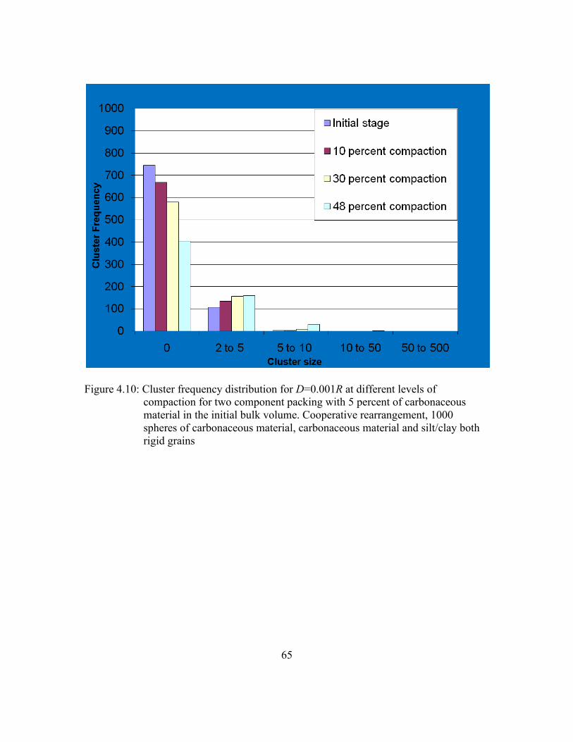
65
Figure 4.10: Cluster frequency distribution for D=0.001R at different levels of
compaction for two component packing with 5 percent of carbonaceous
material in the initial bulk volume. Cooperative rearrangement, 1000
spheres of carbonaceous material, carbonaceous material and silt/clay both
rigid grains

66
Figure 4.11: Number of spheres distribution for D=0.001R at different levels of
compaction for two component packing with 5 percent of carbonaceous
material in the initial bulk volume. Cooperative rearrangement, 1000
spheres of carbonaceous material, carbonaceous material and silt/clay both
rigid grains.
Table 4.3: Cluster frequency distribution for D=0.001R at different levels of compaction
of two component packing with 10 percent of carbonaceous material in the
initial bulk volume. Cooperative rearrangement, 1000 spheres of
carbonaceous material, carbonaceous material and silt/clay both rigid grains.
Compaction
stage Porosity Max cluster size
Normalized
max cluster
size Frequency of clusters by size
0 2 to 5 5 to 10 10 to 50 50 to 500
Initial 0.6973 17 0.017782 461 143 15 3 0
0.9 0.6637 17 0.017782 420 145 23 3 0
0.7 0.5676 32 0.033473 339 147 24 6 0
0.52 0.4179 135 0.141213 170 70 24 13 2

67
Table 4.4: Number of spheres distribution for D=0.001R at different levels of compaction
of two component packing with 10 percent of carbonaceous material in the
initial bulk volume. Cooperative rearrangement, 1000 spheres of
carbonaceous material, carbonaceous material and silt/clay both rigid grains.
Compaction
stage Porosity
Max cluster
size
Normalized
max cluster
size
Total number of spheres in
clusters of different size ranges
0
2 to
5
5 to
10
10 to
50
50 to
500
Initial 0.6973 17 0.017782 461 351 99 45 0
0.9 0.6637 17 0.017782 420 348 143 45 0
0.7 0.5676 32 0.033473 339 374 150 93 0
0.52 0.4179 135 0.141213 170 185 155 204 242

68
Figure 4.12: Cluster frequency distribution for D=0.001R at different levels of
compaction of two component packing with 10 percent of carbonaceous
material in the initial bulk volume. Cooperative rearrangement, 1000
spheres of carbonaceous material, carbonaceous material and silt/clay both
rigid grains.

69
Figure 4.13: Number of spheres distribution for D=0.001R at different levels of
compaction of two component packing with 10 percent of carbonaceous
material in the initial bulk volume. Cooperative rearrangement, 1000
spheres of carbonaceous material, carbonaceous material and silt/clay both
rigid grains.
4.3.2 BOTH CARBONACEOUS AND SILT/CLAY GRAINS ARE DUCTILE
Under this scenario, both carbonaceous material and silt/clay grains are assumed
ductile. Grain packing is subjected to compaction, and both cluster frequency and
number of spheres vs. cluster size are plotted in Figure 4.14-4.17 and summarized in
Table 4.5-4.8. The grain packing of prescribed porosity 70% is compacted to 56% (c=
0.44) for 0.9 rigid radius, 62% (c= 0.38) for 0.8 rigid radius and 68% (c= 0.32) for 0.7
rigid radius giving final residual porosity ~42%, ~23% and ~13% respectively.

70
The final volume fraction of carbonaceous material for initial volume fractions of
5% and 10% of carbonaceous material is 11.3% and 22.7% for 0.9 rigid radius, 13.1%
and 26.3% for 0.8 rigid radius and 15.6% and 31.2% for 0.7 rigid radius
respectively(Table 4.5-4.16 and Figure 4.14-4.25).
It is observed that as the compaction increases, the number of large clusters
increases but the effect of compaction on connectivity of carbonaceous material is more
pronounced as the grains are ductile in this scenario.
Table 4.5: Cluster frequency distribution for D=0.001R at different levels of compaction
of two component packing with 5 percent of carbonaceous material in the
initial bulk volume. Cooperative rearrangement, 1000 spheres of
carbonaceous material, carbonaceous material and silt/clay both ductile
grains with rigid ratio =0.9R
Compaction
stage Porosity
Max
cluster
size
Normalized max
cluster size Frequency of clusters by size
0 2 to 5 5 to 10 10 to 50 50 to 500
Initial 0.7003 8 0.0079 586 165 5 0 0
0.9 0.6639 8 0.0079 546 173 9 0 0
0.7 0.5717 11 0.0108 472 169 20 1 0
0.5 0.3948 17 0.0167 354 155 34 4 0
0.44 0.3178 29 0.0285 304 140 29 12 0

71
Table 4.6: Number of spheres distribution for D=0.001R at different levels of compaction
of two component packing with 5 percent of carbonaceous material in the
initial bulk volume. Cooperative rearrangement, 1000 spheres of
carbonaceous material, carbonaceous material and silt/clay both ductile
grains with rigid ratio =0.9R
Compaction
stage Porosity
Max
cluster
size
Normalized
max cluster
size
Total number of spheres in clusters of
different size ranges
0 2 to 5 5 to 10 10 to 50 50 to 500
Initial 0.7003 8 0.0079 586 402 29 0 0
0.9 0.6639 8 0.0079 546 421 50 0 0
0.7 0.5717 11 0.0108 472 410 124 11 0
0.52 0.3948 17 0.0167 354 400 214 49 0
0.44 0.3178 29 0.0285 352 352 184 177 0

72
Figure 4.14: Cluster frequency distribution for D=0.001R at different levels of
compaction of two component packing with 5 percent of carbonaceous
material in the initial bulk volume. Cooperative rearrangement, 1000
spheres of carbonaceous material, carbonaceous material and silt/clay both
ductile grains with rigid radius ratio =0.9R

73
Figure 4.15: Number of spheres distribution for D=0.001R at different levels of
compaction of two component packing with 5 percent of carbonaceous
material in the initial bulk volume. Cooperative rearrangement, 1000
spheres of carbonaceous material, carbonaceous material and silt/clay both
ductile grains with rigid ratio=0.9R

74
Table 4.7: Cluster frequency distribution for D=0.001R at different levels of compaction
of two component packing with 10 percent of carbonaceous material in the
initial bulk volume. Cooperative rearrangement, 1000 spheres of
carbonaceous material, carbonaceous material and silt/clay both ductile
grains with rigid ratio =0.9R
Compaction
stage Porosity
Max
cluster
size
Normalized max
cluster size Frequency of clusters by size
0 2 to 5 5 to 10 10 to 50 50 to 500
Initial 0.6978 22 0.0218 395 151 30 3 0
0.9 0.6646 21 0.0209 359 147 30 6 0
0.7 0.5691 45 0.0447 255 95 48 10 0
0.5 0.3927 557 0.5531 124 39 12 10 1
0.44 0.3116 798 0.7925 68 20 7 2 1
Table 4.8: Number of spheres distribution for D=0.001R at different levels of compaction
of two component packing with 10 percent of carbonaceous material in the
initial bulk volume. Cooperative rearrangement, 1000 spheres of
carbonaceous material, carbonaceous material and silt/clay both ductile
grains with rigid ratio =0.9R
Compaction
stage Porosity
Max
cluster
size
Normalized
max cluster
size
Total number of spheres in clusters of
different size ranges
0 2 to 5 5 to 10 10 to 50 50 to 500
Initial 0.6978 22 0.0218 395 382 186 44 0
0.9 0.6646 21 0.0209 359 380 181 87 0
0.7 0.5691 45 0.0447 255 251 312 189 0
0.52 0.3927 557 0.5531 124 100 71 155 557
0.44 0.3116 798 0.7925 68 50 42 49 798
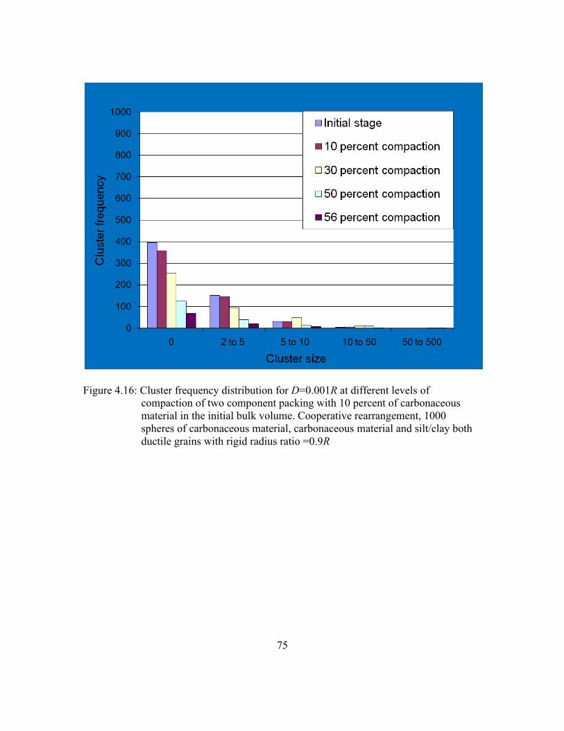
75
Figure 4.16: Cluster frequency distribution for D=0.001R at different levels of
compaction of two component packing with 10 percent of carbonaceous
material in the initial bulk volume. Cooperative rearrangement, 1000
spheres of carbonaceous material, carbonaceous material and silt/clay both
ductile grains with rigid radius ratio =0.9R

76
Figure 4.17: Number of spheres distribution for D=0.001R at different levels of
compaction of two component packing with 10 percent of carbonaceous
material in the initial bulk volume. Cooperative rearrangement, 1000
spheres of carbonaceous material, carbonaceous material and silt/clay both
ductile grains with rigid ratio=0.9R

77
Table 4.9: Cluster frequency distribution for D=0.001R at different levels of compaction
of two component packing with 5 percent of carbonaceous material in the
initial bulk volume. Cooperative rearrangement, 1000 spheres of
carbonaceous material, carbonaceous material and silt/clay both ductile
grains with rigid ratio =0.8R
Compaction
stage Porosity
Max
cluster
size
Normalized max
cluster size Frequency of clusters by size
0 2 to 5 5 to 10 10 to 50 50 to 500
Initial 0.7032 5 0.0050 633 153 3 0 0
0.9 0.6702 6 0.0060 602 160 5 0 0
0.7 0.5759 10 0.0101 541 162 10 1 0
0.5 0.4115 15 0.0151 375 175 24 3 0
0.38 0.2300 33 0.0333 241 118 48 8 0
Table 4.10: Number of spheres distribution for D=0.001R at different levels of
compaction of two component packing with 5 percent of carbonaceous
material in the initial bulk volume. Cooperative rearrangement, 1000
spheres of carbonaceous material, carbonaceous material and silt/clay both
ductile grains with rigid ratio =0.8R
Compaction
stage Porosity
Max
cluster
size
Normalized
max cluster
size
Total number of spheres in clusters of
different size ranges
0 2 to 5 5 to 10 10 to 50 50 to 500
Initial 0.7032 5 0.0050 633 344 15 0 0
0.9 0.6702 6 0.0060 602 364 26 0 0
0.7 0.5759 10 0.0101 541 386 55 1 0
0.5 0.4115 15 0.0151 375 447 134 3 0
0.38 0.2300 33 0.0333 241 315 306 8 0

78
Figure 4.18: Cluster frequency distribution for D=0.001R at different levels of
compaction of two component packing with 5 percent of carbonaceous
material in the initial bulk volume. Cooperative rearrangement, 1000
spheres of carbonaceous material, carbonaceous material and silt/clay both
ductile grains with rigid radius ratio =0.8R

79
Figure 4.19: Number of spheres distribution for D=0.001R at different levels of
compaction of two component packing with 5 percent of carbonaceous
material in the initial bulk volume. Cooperative rearrangement, 1000
spheres of carbonaceous material, carbonaceous material and silt/clay both
ductile grains with rigid ratio=0.8R

80
Table 4.11: Cluster frequency distribution for D=0.001R at different levels of compaction
of two component packing with 10 percent of carbonaceous material in the
initial bulk volume. Cooperative rearrangement, 1000 spheres of
carbonaceous material, carbonaceous material and silt/clay both ductile
grains with rigid ratio =0.8R
Compaction
stage Porosity
Max
cluster
size
Normalized max
cluster size Frequency of clusters by size
0 2 to 5 5 to 10 10 to 50 50 to 500
Initial 0.7056 14 0.0144 380 162 26 2 0
0.9 0.6714 14 0.0144 352 156 30 3 0
0.7 0.5744 30 0.0309 237 123 43 10 0
0.5 0.4120 97 0.0999 125 62 22 15 3
0.38 0.2329 846 0.8713 38 19 5 1 1
Table 4.12: Number of spheres distribution for D=0.001R at different levels of
compaction of two component packing with 10 percent of carbonaceous
material in the initial bulk volume. Cooperative rearrangement, 1000
spheres of carbonaceous material, carbonaceous material and silt/clay both
ductile grains with rigid ratio =0.8R
Compaction
stage Porosity
Max
cluster
size
Normalize
d max
cluster size
Total number of spheres in clusters of
different size ranges
0 2 to 5 5 to 10 10 to 50 50 to 500
Initial 0.7056 14 0.0144 380 407 160 24 0
0.9 0.6714 14 0.0144 352 396 186 37 0
0.7 0.5744 30 0.0309 237 317 272 145 0
0.5 0.4120 97 0.0999 125 166 143 288 249
0.38 0.2329 846 0.8713 38 48 29 10 846

81
Figure 4.20: Cluster frequency distribution for D=0.001R at different levels of
compaction of two component packing with 10 percent of carbonaceous
material in the initial bulk volume. Cooperative rearrangement, 1000
spheres of carbonaceous material, carbonaceous material and silt/clay both
ductile grains with rigid radius ratio =0.8R

82
Figure 4.21: Number of spheres distribution for D=0.001R at different levels of
compaction of two component packing with 10 percent of carbonaceous
material in the initial bulk volume. Cooperative rearrangement, 1000
spheres of carbonaceous material, carbonaceous material and silt/clay both
ductile grains with rigid ratio=0.8R

83
Table 4.13: Cluster frequency distribution for D=0.001R at different levels of compaction
of two component packing with 5 percent of carbonaceous material in the
initial bulk volume. Cooperative rearrangement, 1000 spheres of
carbonaceous material, carbonaceous material and silt/clay both ductile
grains with rigid ratio =0.7R
Compaction
stage Porosity
Max
cluster
size
Normalized max
cluster size Frequency of clusters by size
0 2 to 5 5 to 10 10 to 50 50 to 500
Initial 0.6974 9 0.0091 627 147 5 0 0
0.9 0.6725 9 0.0091 608 150 7 0 0
0.7 0.5814 11 0.0112 543 161 8 1 0
0.5 0.4134 15 0.0152 414 171 16 4 0
0.32 0.1315 27 0.0274 190 119 32 18 0
Table 4.14: Number of spheres distribution for D=0.001R at different levels of
compaction of two component packing with 5 percent of carbonaceous
material in the initial bulk volume. Cooperative rearrangement, 1000
spheres of carbonaceous material, carbonaceous material and silt/clay both
ductile grains with rigid ratio =0.7R
Compaction
stage Porosity
Max
cluster
size
Normalized
max cluster
size
Total number of spheres in clusters of
different size ranges
0 2 to 5 5 to 10 10 to 50 50 to 500
Initial 0.6974 9 0.0091 627 327 30 0 0
0.9 0.6725 9 0.0091 608 334 42 0 0
0.7 0.5814 11 0.0112 543 381 49 11 0
0.5 0.4134 15 0.0152 414 428 93 49 0
0.32 0.1315 27 0.0274 190 316 211 267 0

84
Figure 4.22: Cluster frequency distribution for D=0.001R at different levels of
compaction of two component packing with 5 percent of carbonaceous
material in the initial bulk volume. Cooperative rearrangement, 1000
spheres of carbonaceous material, carbonaceous material and silt/clay both
ductile grains with rigid radius ratio =0.7R

85
Figure 4.23: Number of spheres distribution for D=0.001R at different levels of
compaction of two component packing with 5 percent of carbonaceous
material in the initial bulk volume. Cooperative rearrangement, 1000
spheres of carbonaceous material, carbonaceous material and silt/clay both
ductile grains with rigid ratio=0.7R

86
Table 4.15: Cluster frequency distribution for D=0.001R at different levels of compaction
of two component packing with 10 percent of carbonaceous material in the
initial bulk volume. Cooperative rearrangement, 1000 spheres of
carbonaceous material, carbonaceous material and silt/clay both ductile
grains with rigid ratio =0.7R
Compaction
stage Porosity
Max
cluster
size
Normalized max
cluster size Frequency of clusters by size
0 2 to 5 5 to 10 10 to 50 50 to 500
Initial 0.7011 19 0.0190 394 163 24 6 0
0.9 0.6678 19 0.0190 352 157 31 6 0
0.7 0.5796 22 0.0220 261 134 39 11 0
0.5 0.4178 53 0.0531 137 82 29 14 3
0.32 0.1318 916 0.9178 31 12 3 0 1
Table 4.16: Number of spheres distribution for D=0.001R at different levels of
compaction of two component packing with 10 percent of carbonaceous
material in the initial bulk volume. Cooperative rearrangement, 1000
spheres of carbonaceous material, carbonaceous material and silt/clay both
ductile grains with rigid ratio =0.7R
Compaction
stage Porosity
Max
cluster
size
Normalized
max cluster
size
Total number of spheres in clusters of
different size ranges
0 2 to 5 5 to 10 10 to 50 50 to 500
Initial 0.7011 19 0.0190 394 403 131 70 0
0.9 0.6678 19 0.0190 352 391 180 75 0
0.7 0.5796 22 0.0220 261 348 230 159 0
0.5 0.4178 53 0.0531 137 216 197 292 156
0.32 0.1318 916 0.9178 31 31 20 0 916

87
Figure 4.24: Cluster frequency distribution for D=0.001R at different levels of
compaction of two component packing with 10 percent of carbonaceous
material in the initial bulk volume. Cooperative rearrangement, 1000
spheres of carbonaceous material, carbonaceous material and silt/clay both
ductile grains with rigid radius ratio =0.7R

88
Figure 4.25: Number of spheres distribution for D=0.001R at different levels of
compaction of two component packing with 10 percent of carbonaceous
material in the initial bulk volume. Cooperative rearrangement, 1000
spheres of carbonaceous material, carbonaceous material and silt/clay both
ductile grains with rigid ratio=0.7R
4.3.3 CARBONACEOUS MATERIAL IS DUCTILE AND SILT/CLAY GRAINS ARE RIGID
Under this scenario, only carbonaceous material is assumed to be ductile. The
grain packing used for the scenario of all the spheres to be rigid was considered for this
analysis which ensured that there was no overlap of spheres in the initial sediment
setting. The grain packing is subjected to compaction and both cluster frequency vs.
cluster size and number of spheres vs. cluster size are plotted in Figure 4.26-4.37 and
summarized in Table 4.17-4.28. It is observed that the grain packing of prescribed

89
porosity 70% is compacted to 50% (c= 0.50) for all the cases (0.9 rigid radius, 0.8 rigid
radius and 0.7 rigid radius) giving a final porosity of approximately 40%. The final
volume fractions of carbonaceous material for initial 5% and 10% volume fraction of
carbonaceous material is 10% and 20% respectively.
The results (Figure 4.26-4.37) shows that as the compaction increases, number of
large cluster increases. However, the effect of compaction on connectivity of
carbonaceous material is less pronounced than the case of both carbonaceous material
and silt/clay grains as ductile grains (Figure 4.13-4.25). There is a minor effect of
ductility of carbonaceous material on connectivity observed in 0.05 and 0.10 volume
fraction of carbonaceous material grain packing (Figure 4.26-4.37).
Table 4.17: Cluster frequency distribution for D=0.001R at different levels of
compaction of two component packing with 5 percent of carbonaceous
material in the initial bulk volume. Cooperative rearrangement, 1000
spheres of carbonaceous material, carbonaceous material being ductile with
rigid radius ratio =0.9R and silt/clay being rigid
Compaction
stage Porosity
Max
cluster
size
Normalized max
cluster size Frequency of clusters by size
0 2 to 5 5 to 10 10 to 50 50 to 500
Initial 0.702984 7 0.0070 744 107 3 0 0
0.9 0.667 5 0.0050 637 144 1 0 0
0.7 0.5664 10 0.0101 492 173 15 1 0
0.5 0.4007 11 0.0111 278 146 43 10 0

90
Table 4.18: Number of spheres distribution for D=0.001R at different levels of
compaction of two component packing with 5 percent of carbonaceous
material in the initial bulk volume. Cooperative rearrangement, 1000
spheres of carbonaceous material, carbonaceous material being ductile with
rigid radius ratio=0.9R and silt/clay being rigid
Compaction
stage Porosity
Max
cluster
size
Normalize
d max
cluster size
Total number of spheres in clusters of
different size ranges
0 2 to 5 5 to 10 10 to 50 50 to 500
Initial 0.7030 7 0.0070 744 233 18 0 0
0.9 0.6670 5 0.0050 637 333 25 0 0
0.7 0.5664 10 0.0101 492 410 83 10 0
0.5 0.4007 11 0.0111 278 382 264 71 0

91
Figure 4.26: Cluster frequency distribution for D=0.001R at different levels of
compaction of two component packing with 5 percent of carbonaceous
material in the initial bulk volume. Cooperative rearrangement, 1000
spheres of carbonaceous material, carbonaceous material being ductile with
rigid radius ratio=0.9R and silt/clay being rigid

92
Figure 4.27: Number of spheres distribution for D=0.001R at different levels of
compaction of two component packing with 5 percent of carbonaceous
material in the initial bulk volume. Cooperative rearrangement, 1000
spheres of carbonaceous material, carbonaceous material being ductile with
rigid radius ratio =0.9R and silt/clay being rigid

93
Table4.19: Cluster frequency distribution for D=0.001R at different levels of compaction
of two component packing with 10 percent of carbonaceous material in the
initial bulk volume. Cooperative rearrangement, 1000 spheres of
carbonaceous material, carbonaceous material being ductile with rigid radius
ratio =0.9R and silt/clay being rigid
Compaction
stage Porosity
Max
cluster
size
Normalized max
cluster size Frequency of clusters by size
0 2 to 5 5 to 10 10 to 50 50 to 500
Initial 0.6975 17 0.0178 432 149 20 2 0
0.9 0.6665 16 0.0167 371 150 26 4 0
0.7 0.5662 43 0.0450 252 127 37 9 0
0.5 0.4021 550 0.5753 83 43 10 9 0
Table 4.20: Number of spheres distribution for D=0.001R at different levels of
compaction of two component packing with 10 percent of carbonaceous
material in the initial bulk volume. Cooperative rearrangement, 1000
spheres of carbonaceous material, carbonaceous material being ductile with
rigid radius ratio=0.9R and silt/clay being rigid
Compaction
stage Porosity
Max
cluster
size
Normalized
max cluster
size
Total number of spheres in clusters of
different size ranges
0 2 to 5 5 to 10 10 to 50 50 to 500
Initial 0.6975 17 0.0178 432 369 133 22 0
0.9 0.6665 16 0.0167 371 367 170 48 0
0.7 0.5662 43 0.0450 252 320 234 150 0
0.5 0.4021 550 0.5753 83 114 60 149 550

94
Figure 4.28: Cluster frequency distribution for D=0.001R at different levels of
compaction of two component packing with 10 percent of carbonaceous
material in the initial bulk volume. Cooperative rearrangement, 1000
spheres of carbonaceous material, carbonaceous material being ductile with
rigid radius ratio=0.9R and silt/clay being rigid

95
Figure 4.29: Number of spheres distribution for D=0.001R at different levels of
compaction of two component packing with 10 percent of carbonaceous
material in the initial bulk volume. Cooperative rearrangement, 1000
spheres of carbonaceous material, carbonaceous material being ductile with
rigid radius ratio =0.9R and silt/clay being rigid

96
Table 4.21: Cluster frequency distribution for D=0.001R at different levels of
compaction of two component packing with 5 percent of carbonaceous
material in the initial bulk volume. Cooperative rearrangement, 1000
spheres of carbonaceous material, carbonaceous material being ductile with
rigid radius ratio =0.8 R and silt/clay being rigid
Compaction
stage Porosity
Max
cluster
size
Normalized max
cluster size Frequency of clusters by size
0 2 to 5 5 to 10 10 to 50 50 to 500
Initial 0.7030 7 0.0070 744 107 3 0 0
0.9 0.6661 5 0.0050 636 149 4 0 0
0.7 0.5676 10 0.0101 498 173 14 1 0
0.5 0.3955 15 0.0151 261 145 48 5 0
Table 4.22: Number of spheres distribution for D=0.001R at different levels of
compaction of two component packing with 5 percent of carbonaceous
material in the initial bulk volume. Cooperative rearrangement, 1000
spheres of carbonaceous material, carbonaceous material being ductile with
rigid radius ratio=0.8R and silt/clay being rigid
Compaction
stage Porosity
Max
cluster
size
Normalized
max cluster
size
Total number of spheres in clusters of
different size ranges
0 2 to 5 5 to 10 10 to 50 50 to 500
Initial 0.7030 7 0.0070 744 233 18 0 0
0.9 0.6661 5 0.0050 636 339 20 0 0
0.7 0.5676 10 0.0101 498 410 77 10 0
0.5 0.3955 15 0.0151 261 377 298 59 0

97
Figure 4.30: Cluster frequency distribution for D=0.001R at different levels of
compaction of two component packing with 5 percent of carbonaceous
material in the initial bulk volume. Cooperative rearrangement, 1000
spheres of carbonaceous material, carbonaceous material being ductile with
rigid radius ratio=0.8R and silt/clay being rigid

98
Figure 4.31: Number of spheres distribution for D=0.001R at different levels of
compaction of two component packing with 5 percent of carbonaceous
material in the initial bulk volume. Cooperative rearrangement, 1000
spheres of carbonaceous material, carbonaceous material being ductile with
rigid radius ratio =0.8R and silt/clay being rigid

99
Table 4.23: Cluster frequency distribution for D=0.001R at different levels of compaction
of two component packing with 10 percent of carbonaceous material in the
initial bulk volume. Cooperative rearrangement, 1000 spheres of
carbonaceous material, carbonaceous material being ductile with rigid radius
ratio =0.8 R and silt/clay being rigid
Compaction
stage Porosity
Max
cluster
size
Normalized max
cluster size Frequency of clusters by size
0 2 to 5 5 to 10 10 to 50 50 to 500
Initial 0.6975 21 0.0220 369 139 26 5 0
0.9 0.6661 14 0.0146 338 147 33 3 0
0.7 0.5636 43 0.0450 211 136 32 12 0
0.5 0.3974 325 0.3400 60 41 15 7 2
Table 4.24: Number of spheres distribution for D=0.001R at different levels of
compaction of two component packing with 10 percent of carbonaceous
material in the initial bulk volume. Cooperative rearrangement, 1000
spheres of carbonaceous material, carbonaceous material being ductile with
rigid radius ratio=0.8R and silt/clay being rigid
Compaction
stage Porosity
Max
cluster
size
Normalized
max cluster
size
Total number of spheres in clusters of
different size ranges
0 2 to 5 5 to 10 10 to 50 50 to 500
Initial 0.6975 21 0.0220 369 347 171 69 0
0.9 0.6661 14 0.0146 338 358 224 36 0
0.7 0.5636 43 0.0450 211 351 204 190 0
0.5 0.3974 325 0.3400 60 111 92 154 539

100
Figure 4.32: Cluster frequency distribution for D=0.001R at different levels of
compaction of two component packing with 10 percent of carbonaceous
material in the initial bulk volume. Cooperative rearrangement, 1000
spheres of carbonaceous material, carbonaceous material being ductile with
rigid radius ratio=0.8R and silt/clay being rigid

101
Figure 4.33: Number of spheres distribution for D=0.001R at different levels of
compaction of two component packing with 10 percent of carbonaceous
material in the initial bulk volume. Cooperative rearrangement, 1000
spheres of carbonaceous material, carbonaceous material being ductile with
rigid radius ratio =0.8R and silt/clay being rigid

102
Table 4.25: Cluster frequency distribution for D=0.001R at different levels of compaction
of two component packing with 5 percent of carbonaceous material in the
initial bulk volume. Cooperative rearrangement, 1000 spheres of
carbonaceous material, carbonaceous material being ductile with rigid radius
ratio =0.7 R and silt/clay being rigid
Compaction
stage Porosity
Max
cluster
size
Normalized
max cluster
size Frequency of clusters by size
0 2 to 5 5 to 10 10 to 50 50 to 500
Initial 0.7030 7 0.0070 744 107 3 0 0
0.9 0.6659 5 0.0050 635 149 4 0 0
0.7 0.5690 10 0.0101 498 174 15 1 0
0.5 0.3982 17 0.0171 262 162 40 5 0
Table 4.26: Number of spheres distribution for D=0.001R at different levels of
compaction of two component packing with 5 percent of carbonaceous
material in the initial bulk volume. Cooperative rearrangement, 1000
spheres of carbonaceous material, carbonaceous material being ductile with
rigid radius ratio=0.7R and silt/clay being rigid
Compaction
stage Porosity
Max
cluster
size
Normalized
max cluster
size
Total number of spheres in clusters of
different size ranges
0 2 to 5 5 to 10 10 to 50 50 to 500
Initial 0.7030 7 0.0070 744 233 18 0 0
0.9 0.6659 5 0.0050 635 340 20 0 0
0.7 0.5690 10 0.0101 498 406 81 10 0
0.5 0.3982 17 0.0171 262 420 249 64 0

103
Figure 4.34: Cluster frequency distribution for D=0.001R at different levels of
compaction of two component packing with 5 percent of carbonaceous
material in the initial bulk volume. Cooperative rearrangement, 1000
spheres of carbonaceous material, carbonaceous material being ductile with
rigid radius ratio=0.7R and silt/clay being rigid

104
Figure 4.35: Number of spheres distribution for D=0.001R at different levels of
compaction of two component packing with 5 percent of carbonaceous
material in the initial bulk volume. Cooperative rearrangement, 1000
spheres of carbonaceous material, carbonaceous material being ductile with
rigid radius ratio =0.7R and silt/clay being rigid

105
Table 4.27: Cluster frequency distribution for D=0.001R at different levels of compaction
of two component packing with 10 percent of carbonaceous material in the
initial bulk volume. Cooperative rearrangement, 1000 spheres of
carbonaceous material, carbonaceous material being ductile with rigid radius
ratio =0.7 R and silt/clay being rigid
Compaction
stage Porosity
Max
cluster
size
Normalized max
cluster size Frequency of clusters by size
0 2 to 5 5 to 10 10 to 50 50 to 500
Initial 0.6975 17 0.0178 432 149 20 2 0
0.9 0.6661 12 0.0126 373 157 28 2 0
0.7 0.5636 21 0.0220 250 142 38 7 0
0.5 0.3974 161 0.1684 78 48 12 14 5
Table 4.28: Number of spheres distribution for D=0.001R at different levels of
compaction of two component packing with 10 percent of carbonaceous
material in the initial bulk volume. Cooperative rearrangement, 1000
spheres of carbonaceous material, carbonaceous material being ductile with
rigid radius ratio=0.7R and silt/clay being rigid
Compaction
stage Porosity
Max
cluster
size
Normalized
max cluster
size
Total number of spheres in clusters of
different size ranges
0 2 to 5 5 to 10 10 to 50 50 to 500
Initial 0.6975 17 0.0178 432 369 133 22 0
0.9 0.6661 12 0.0126 373 381 180 22 0
0.7 0.5636 21 0.0220 250 359 244 103 0
0.5 0.3974 161 0.1684 78 130 79 232 437

106
Figure 4.36: Cluster frequency distribution for D=0.001R at different levels of
compaction of two component packing with 10 percent of carbonaceous
material in the initial bulk volume. Cooperative rearrangement, 1000
spheres of carbonaceous material, carbonaceous material being ductile with
rigid radius ratio=0.7R and silt/clay being rigid

107
Figure 4.37: Number of spheres distribution for D=0.001R at different levels of
compaction of two component packing with 10 percent of carbonaceous
material in the initial bulk volume. Cooperative rearrangement, 1000
spheres of carbonaceous material, carbonaceous material being ductile with
rigid radius ratio =0.7R and silt/clay being rigid
4.4 RELATIONSHIP OF CLUSTER STATISTICS TO POROSITY
Cluster statistics generated in the previous section for all the three scenarios were
analyzed and related to the porosity values of the grain packing for 5 and 10 percent of
carbonaceous material, considering all grains rigid, all grains ductile with rigid radius
ratios of 0.9, 0.8 and 0.7 and only carbonaceous material ductile with rigid ratios of 0.9,
0.8 and 0.7 with target porosity of 70% as shown in plots in Figure 4.38-4.41. A
relationship between porosity and number of clusters and porosity and number of spheres
in different cluster sizes is observed. Isolated grains and small cluster sizes 2 to 5

108
decreased with decrease in porosity while large cluster size 5 to 10 and 10 to 50 increased
with decrease in porosity for 5 percent and 10 percent of carbonaceous material by bulk
volume grain packing of the scenarios discussed in the previous section. A porosity of
0.40 was observed as a critical point for clustering for the packing having 10 percent of
carbonaceous for the above scenarios which corresponded to 50% of compaction.
Figure 4.38: Relationship between number of clusters and sediment porosity with 5
percent of carbonaceous material in the initial bulk volume for initial
sediment porosity of 70%. Values taken from Table 4.1, Table 4.5, Table
4.9, Table 4.13, Table 4.17, Table 4.21, Table 4.25

109
Figure 4.39: Relationship between number of spheres in cluster size and sediment
porosity with 5 percent of carbonaceous material in the initial bulk volume
for initial porosity 70%.Values taken from Table 4.2, Table 4.6, Table 4.10,
Table 4.14, Table 4.18, Table 4.22, Table 4.26

110
Figure 4.40: Relationship between number of clusters and sediment porosity with 10
percent of carbonaceous material in the initial bulk volume for initial
porosity of 70%.Values taken from Table 4.3, Table 4.7, Table 4.11, Table
4.15, Table 4.19, Table 4.23, Table 4.27

111
Figure 4.41: Relationship between number of spheres in cluster size and sediment
porosity with 10 percent of carbonaceous material in the initial bulk volume
for initial porosity of 70%.Values taken from Table 4.4, Table 4.8, Table
4.12, Table 4.16, Table 4.20, Table 4.24, Table 4.28
4.5 DISCUSSION OF CLUSTERING TRENDS
The results discussed in the previous section 4.3 have significant implications for
the mudrock system. In the scenario of all the spheres to be rigid (section 4.3.1), for 5
percent of carbonaceous material by bulk volume and for 48 percent compaction, the
cluster frequency distribution plot show only 31 big clusters in cluster size 5-10 and 10
to 50 as shown in Figure 4.10. However the number of spheres associated with these
classes is 190 which is 20 percent of all the spheres of carbonaceous material as shown

112
in Figure 4.11. Similarly, for 10 percent of carbonaceous material as shown in Figure
4.13, the number of spheres associated with cluster size 5-10, 10-50 and 50-500
collectively are around 601 which is 60 percent of all the spheres of carbonaceous
material.
Ductility of grains plays an important role in the connectivity of organic material
in mudrocks which was studied in section 4.3.2 and 4.3.3. For 5 percent of carbonaceous
material by bulk volume at last compaction stage, the total number of spheres associated
with cluster sizes 5-10 and 10-50 is 361 with ductility of rigid radius ratio 0.9 R, 314
with ductility of rigid radius ratio 0.8R and 478 with ductility of rigid radius ratio 0.7R
which is in a range of 30-50 % of the total carbonaceous material. For 10 percent of
carbonaceous material by bulk volume at last compaction stage, the number of spheres
associated with cluster size 5-10, 10-50 and 50-500 is 889 with ductility of rigid radius
ratio 0.9 R, 885 with ductility of rigid radius ratio 0.8R and 936 with ductility of rigid
radius ratio 0.7R which is in a range of 80-95 % of the total carbonaceous material.
Thus these results show the significant effect of burial and compaction on
clustering of organic material in mudrocks which is important for evaluating the resource
quality.

113
Chapter 5: Conclusions and Future directions
5.1 CONCLUSIONS
This study suggests a mechanism whereby small amounts of carbonaceous
material can occur not as just isolated grains but as connected clusters of grains within a
mudrock. This supports the hypothesis that gas production from mudrock is along the
connected paths within the carbonaceous material. The study focuses on the dependence
of the statistics of the clusters upon volume fraction of carbonaceous material and degree
of compaction. The dependence can be useful for estimating the resource quality.
Volume fraction of carbonaceous material has a significant effect on the
clustering statistics. In the model sediment, the number and size of carbonaceous clusters
are small, but they increase with increase in volume fraction of carbonaceous material
(Figure 3.5-3.8). The grain packing reaches to a maximum number of clusters after which
two or more distinct small clusters merge to form a big cluster. This phenomenon
happens at 0.20 volume fraction of carbonaceous material which only happens with
cooperative rearrangement algorithm which induces clustering. The big cluster continues
to grow and eventually all the spheres of the packing touch each other to form one
cluster.
Degree of compaction is identified as one more important factor controlling the
cluster statistics. The numbers of clusters start increasing in number and size with
increase in degree of compaction (c) and at a 50% compaction stage a significantly large
cluster is formed which may lead to percolation (Figure 4.1-4.12). However, there is less
clustering of spheres if in initial sediment carbonaceous material is forced apart.

114
Ductility of grains is another important aspect of this study. With the same
volume fraction of carbonaceous material, ductility enhances the connectivity of
carbonaceous material in mudrocks. The connectivity of carbonaceous material with
compaction increases more in scenario of both carbonaceous material and silt/clay ductile
than of only carbonaceous material being ductile (Figure 4.13-4.36).
5.2 FUTURE DIRECTIONS
In general a reevaluation of the assumptions is needed in order to gain insight into
the clustering mechanism. If after the revision the model succeeds, then it motivates
further testing and validation through experiments.
Even if the grain packing of almost same size spheres captures the random spatial
arrangements of grains in sediments, they are an oversimplification of grains naturally
occurring in sediments. Therefore, these packings are not always representative of a
physical system. A next step would be to study the cluster distribution of carbonaceous
material with aspect ratios between the sizes of carbonaceous material and silt/clay.
In this study, grains are assumed to be spherical. It would be instructive to study
the connectivity of carbonaceous material if these were angular or some random shape.
This study may bring out any effect of shape on the connectivity of sediments.
A further extension of the current work can be taking the grain packing forward to
commercial simulator for studying the multiphase effect on the gas permeability in
mudrocks.

115
Figure 5.1: Schematic diagram showing the roadmap of taking grain packing forward to
commercial simulator for studying multiphase effect on gas phase
permeability in mudrocks.

116
Appendix
CODES
Some of the codes used in this thesis are showed in this appendix. Many of these
codes refer to specific data files. Contact the author at email
[email protected] for more information.
Code for compaction with cooperative rearrangement
parameter (MAX =30000)
real array1(MAX,5)
real array(MAX,5),cm(MAX),cv(MAX), newarray(MAX,5)
real compaction, step, grainvolume,porosity,ff,gg
integer counter, iteration,ak,bk,sd,pin(MAX),ii,pinflag(MAX)
logical qq, ww, ee
real xx,yy,zz,mincomp,maxrad
integer p
real rb, rs
write(*,*)' Number of Spheres'
read(*,*)p
write(*,*)' Radius of big spheres'
read(*,*)rb
write(*,*)' Radius of small spheres'
read(*,*)rs
write(*,*) ' Compaction Step'
step =0.02
maxrad = 0
ductility = 0.35
open(5, file='new.txt' , status ='UNKNOWN')
!$$$$$$ reading the input file
do i = 1,p
read(5,*) array1(i,1:5)
if(maxrad.lt.array1(i,5)) maxrad = array1(i,5)
end do
close(5)
open(2, file='results.txt' , status ='UNKNOWN')
compaction = 1
array =0

117
do i = 1,p
array(i,1) =array1(i,1)
array(i,2)= array1(i,2)
array(i,3)=array1(i,3)
array(i,4)=array1(i,4)
array(i,5)=array1(i,5)
enddo
!Compaction loop
mincomp = (2*maxrad/70)+0.01
77 compaction = compaction -step
if (compaction.lt.mincomp) compaction = mincomp
! Initialization of the array containing spheres
do ii = 1,p
array(ii,2)= array(ii,2)*compaction/(compaction+step)
enddo
!-------------Making of Conjugates------------------------------------------------
array(p+1:MAX,:) =0
call conjugate(p,array,mp,pin,compaction,pinflag)
write(1,*) mp
counter = 1
iteration=0
do while(counter.gt.0 .and. iteration.lt.250)
iteration = iteration +1
write(1,*) 'Overlaps', counter
counter =0
write(2,*) 'Iteration', iteration
write(1,*) 'Iteration', iteration
do ak= 1,mp
do bk = 1,mp
if(ak.ne.bk)then
d = ((array(ak,2)- array(bk,2))**2 + (array(ak,3)- array(bk,3))**2+(array(ak,4)-
array(bk,4))**2)**0.5
if( array(ak,5).eq.rb .and. array(bk,5) .eq. rb)then
overlap = array(ak,5)+array(bk,5)- d
overlap = overlap - ductility *((array(ak,5)+array(bk,5))/2)
else
overlap = array(ak,5)+array(bk,5)- d
endif
if (overlap.gt. 0.01) then
!---------------------------Removal of overlap----------------------------------------------

118
counter = counter
dx= abs(array(ak,2)- array(bk,2))
dy=abs(array(ak,3)- array(bk,3))
dz= abs(array(ak,4)- array(bk,4))
!----- X direction -------------------------------------------------------------------
xx = overlap*dx/(2*d)
yy = overlap*dy/(2*d)
zz = overlap*dz/(2*d)
if (array(ak,2).gt.array(bk,2) )then
array(ak,2)= array(ak,2) + xx
array(bk,2)= array(bk,2) - xx
else
array(ak,2)= array(ak,2) - xx
array(bk,2)= array(bk,2) + xx
xx= -xx
endif
!------ Y direction-----------------------------------------------------------------------
if (array(ak,3).gt.array(bk,3))then
array(ak,3)= array(ak,3) + yy
array(bk,3)= array(bk,3) - yy
else
array(ak,3)= array(ak,3) - yy
array(bk,3)= array(bk,3) + yy
yy = -yy
endif
!--------- Z direction----------------------------------------------------------------------
if (array(ak,4).gt.array(bk,4))then
array(ak,4)= array(ak,4) + zz
array(bk,4)= array(bk,4) - zz
else
array(ak,4)= array(ak,4) - zz
array(bk,4)= array(bk,4) + zz
zz = -zz
endif
!-------------MOVE CONJUGATES--------------------------------------------------------
if ( pinflag(ak).eq.1 ) then
array(pin(ak),2) = array(pin(ak),2)+xx ; array(pin(ak),3)=array(pin(ak),3)+yy
array(pin(ak),4) = array(pin(ak),4) +zz
endif
if ( pinflag(bk).eq.1 ) then
array(pin(bk),2) = array(pin(bk),2)-xx ; array(pin(bk),3)=array(pin(bk),3)-yy
array(pin(bk),4) = array(pin(bk),4) -zz

119
endif
if ( pinflag(ak).eq.2 ) then
if(ak.le.p) then
do i = 0,2
array(pin(ak)+i,2)=array(pin(ak)+i,2)+xx
array(pin(ak)+i,3)=array(pin(ak)+i,3)+yy
array(pin(ak)+i,4) = array(pin(ak)+i,4) +zz
end do
else
array(pin(ak),2) = array(pin(ak),2)+xx ; array(pin(ak),3)=array(pin(ak),3)+yy
array(pin(ak),4) = array(pin(ak),4) +zz
do i = -2,2
if( (i.ne.0).and.(pin(ak+i).eq.pin(ak)) ) then
array(ak+i,2) = array(ak+i,2)+xx ; array(ak+i,3)=array(ak+i,3)+yy
array(ak+i,4) = array(ak+i,4) +zz
end if
end do
end if
end if
if ( pinflag(bk).eq.2 ) then
if(bk.le.p) then
do i = 0,2
array(pin(bk)+i,2)=array(pin(bk)+i,2)-xx
array(pin(bk)+i,3)=array(pin(bk)+i,3)-yy
array(pin(bk)+i,4) = array(pin(bk)+i,4) - zz
end do
else
array(pin(bk),2) = array(pin(bk),2)- xx ; array(pin(bk),3)=array(pin(bk),3)- yy
array(pin(bk),4) = array(pin(bk),4) -zz
do i = -2,2
if( (i.ne.0).and.(pin(bk+i).eq.pin(bk)) ) then
array(bk+i,2) = array(bk+i,2)- xx ; array(bk+i,3)=array(bk+i,3)- yy
array(bk+i,4) = array(bk+i,4) - zz
end if
end do
end if
end if
if ( pinflag(ak).eq.3 ) then
if(ak.le.p) then
do i = 0,6
array(pin(ak)+i,2)=array(pin(ak)+i,2)+xx
array(pin(ak)+i,3)=array(pin(ak)+i,3)+yy
120
array(pin(ak)+i,4) = array(pin(ak)+i,4) +zz
end do
else
array(pin(ak),2) = array(pin(ak),2)+xx ; array(pin(ak),3)=array(pin(ak),3)+yy
array(pin(ak),4) = array(pin(ak),4) +zz
do i = -6,6
if( (i.ne.0).and.(pin(ak+i).eq.pin(ak)) ) then
array(ak+i,2) = array(ak+i,2)+xx ; array(ak+i,3)=array(ak+i,3)+yy
array(ak+i,4) = array(ak+i,4) +zz
end if
end do
end if
end if
if ( pinflag(bk).eq.3 ) then
if(bk.le.p) then
do i = 0,6
array(pin(bk)+i,2)=array(pin(bk)+i,2)-xx
array(pin(bk)+i,3)=array(pin(bk)+i,3)-yy
array(pin(bk)+i,4) = array(pin(bk)+i,4) - zz
end do
else
array(pin(bk),2) = array(pin(bk),2)- xx
array(pin(bk),3)=array(pin(bk),3)- yy
array(pin(bk),4) = array(pin(bk),4) -zz
do i = -6,6
if( (i.ne.0).and.(pin(bk+i).eq.pin(bk)) ) then
array(bk+i,2) = array(bk+i,2)- xx ; array(bk+i,3)=array(bk+i,3)- yy
array(bk+i,4) = array(bk+i,4) - zz
end if
end do
end if
end if
!-------------Making of Conjugates Again before finding next overlap----------------
newarray =0
do ii = 1,p
qq = (array(ii,2).gt.0).and.(array(ii,2).lt.70*compaction)
ww = (array(ii,3).gt.0).and.(array(ii,3).lt.70)
ee = (array(ii,4).gt.0).and.(array(ii,4).lt.70)
if ( (.not.qq).and.(.not.ww).and.(.not.ee) ) then
newarray(ii,1:5) = array(pin(ii),1:5)
else

121
newarray(ii,:) = array(ii,:)
endif
end do
array = newarray
call conjugate(p,array,mp,pin,compaction,pinflag)
endif
endif
end do
end do
write(1,*)'Number of spheres including conjugates', mp
write(2,*) counter
end do
!--------------------------------------------calculation for volume of overlap-------------
if (iteration .lt.250.or.counter.lt.mp*0.01) then
write(2,*) ' Compaction Step',compaction
do i = 1,mp
write(2,'(2i8,5F15.4)')pinflag(i),
pin(i),array(i,1),array(i,2),array(i,3),array(i,4),array(i,5)
end do
if(compaction.gt.mincomp) go to 77
endif
write(2,*)"Compaction not possible at the stage", compaction
end program
!------------------------------- Subroutine of calculation of Conjugates ----------------
subroutine conjugate(p,array,mp,pin,compaction,pinflag)
real array(30000,5),compaction
integer p, mp,tk,pin(30000),pinflag(30000)
logical aax, aay, aaz, bbx,bby,bbz,check
real xx,yy,zz
pinflag =0
mp = p
pin =0
do tk = 1,p
aax= (array(tk,2)-array(tk,5)).lt.0
aay = (array(tk,3)-array(tk,5)).lt.0
aaz= (array(tk,4)-array(tk,5)).lt.0
bbx = (array(tk,2)+array(tk,5)).gt.70*compaction
bby = (array(tk,3)+array(tk,5)).gt.70
bbz= (array(tk,4)+array(tk,5)).gt.70
! Xdirection LHS

122
if (aax .and. (.not.aay).and.(.not.bby).and.(.not.bbz).and.( .not.aaz) )then
mp = mp+1
array(mp,1)= mp
array(mp,2) = array(tk,2)+ 70*compaction
array(mp,3) = array(tk,3)
array(mp,4)=array(tk,4)
array(mp,5)=array(tk,5)
pin(tk)= mp
pin(mp) = tk
pinflag(tk)=1;pinflag(mp)=1
endif
! Xdirection RHS
if (bbx .and.(.not.aay).and.(.not.bby).and.(.not.aaz).and. (.not. bbz) )then
mp = mp+1
array(mp,1) = mp
array(mp,2) = array(tk,2)- 70*compaction
array(mp,3) = array(tk,3)
array(mp,4)=array(tk,4)
array(mp,5)=array(tk,5)
pin(tk)=mp
pin(mp) =tk
pinflag(tk)=1;pinflag(mp)=1
endif
! Y direction LHS
if (aay .and. (.not.aax) .and.(.not.bbx).and.(.not.bbz).and. (.not.aaz) )then
mp = mp+1
array(mp,1)= mp
array(mp,2) = array(tk,2)
array(mp,3) = array(tk,3)+ 70
array(mp,4)=array(tk,4)
array(mp,5)=array(tk,5)
pin(tk)=mp
pin(mp) =tk
pinflag(tk)=1;pinflag(mp)=1
endif
! Y direction RHS
if (bby .and. (.not.aax).and.(.not.bbx) .and.(.not.aaz).and.(.not. bbz))then
mp = mp+1
array(mp,1)= mp
array(mp,2) = array(tk,2)
array(mp,3) = array(tk,3)- 70
array(mp,4)=array(tk,4)
array(mp,5)=array(tk,5)

123
pin(tk)= mp
pin(mp)=tk
pinflag(tk)=1;pinflag(mp)=1
endif
! Z direction LHS
if (aaz .and. (.not.aax) .and.(.not.bbx).and. (.not.bby).and. (.not.aay) )then
mp = mp+1
array(mp,1) = mp
array(mp,2) = array(tk,2)
array(mp,3) = array(tk,3)
array(mp,4)=array(tk,4)+ 70
array(mp,5)=array(tk,5)
pin(tk)=mp
pin(mp)=tk
pinflag(tk)=1;pinflag(mp)=1
endif
! Z direction RHS
if (bbz .and. (.not.bbx) .and. (.not.aax).and. (.not.aay).and.(.not. bby) )then
mp = mp+1
array(mp,1)= mp
array(mp,2) = array(tk,2)
array(mp,3) = array(tk,3)
array(mp,4)=array(tk,4)- 70
array(mp,5)=array(tk,5)
pin(tk)=mp
pin(mp)=tk
pinflag(tk)=1;pinflag(mp)=1
endif
!-------------------------MAKING CONJUGATES FOR EDGES-----------------------
! X direction edge1
if (aax .and. aay .and.(.not.bbz).and. (.not.aaz) )then
mp = mp+1
array(mp,:) = array(tk,:); array(mp,1) = mp
array(mp,2) = array(mp,2)+ 70*compaction ;array(mp,3) = array(mp,3)+70
pin(tk)= mp; pin(mp) = tk
pinflag(tk) = 2;pinflag(mp)=2
mp = mp +1
array(mp,:) = array(tk,:)
array(mp,1) = mp; array(mp,2) = array(mp,2)+ 70*compaction
pin(mp) = tk ; pinflag(mp)=2
mp = mp +1

124
array(mp,:) = array(tk,:); array(mp,1) = mp;array(mp,3) = array(mp,3)+70
pin(mp) = tk
pinflag(mp)=2
endif
! X direction edge2
if (aax .and. (.not.bby).and.(.not.aay) .and. aaz)then
mp = mp+1
array(mp,:) = array(tk,:); array(mp,1) = mp
array(mp,2) = array(tk,2)+ 70*compaction ;array(mp,4)=array(tk,4)+70
pin(tk)= mp ;pin(mp) = tk; pinflag(tk) = 2;pinflag(mp)=2
mp = mp +1
array(mp,:) =array(tk,:)
array(mp,1) = mp; array(mp,2) = array(mp,2)+ 70*compaction
pin(mp) = tk ; pinflag(mp)=2
mp = mp +1
array(mp,:) = array(tk,:); array(mp,1) = mp; array(mp,4)=array(mp,4)+70
pin(mp) = tk ; pinflag(mp)=2
endif
! Xdirection edge3
if (aax .and. bby .and.(.not.bbz).and. (.not.aaz) )then
mp = mp+1
array(mp,:) = array(tk,:); array(mp,1) = mp
array(mp,2) = array(tk,2)+ 70*compaction ;array(mp,3) = array(mp,3)-70
pin(tk)= mp ;pin(mp) = tk; pinflag(tk) = 2;pinflag(mp)=2
mp = mp+1
array(mp,:) = array(tk,:)
array(mp,1) = mp; array(mp,2) = array(mp,2)+ 70*compaction
pin(mp) = tk ; pinflag(mp)=2
mp = mp+1
array(mp,:) = array(tk,:); array(mp,1) = mp; array(mp,3) = array(mp,3)-70
pin(mp) = tk ; pinflag(mp)=2
endif
! X direction edge4
if (aax .and. (.not.bby) .and.(.not.aay).and. bbz)then
mp = mp+1
array(mp,:) = array(tk,:); array(mp,1) = mp
array(mp,2) = array(tk,2)+ 70*compaction; array(mp,4)=array(mp,4)-70
pin(tk)= mp ;pin(mp) = tk; pinflag(tk) = 2;pinflag(mp)=2
mp = mp+1
array(mp,:) = array(tk,:)
array(mp,1) = mp; array(mp,2) = array(mp,2)+ 70*compaction
pin(mp) = tk ; pinflag(mp)=2
mp = mp+1

125
array(mp,:) = array(tk,:); array(mp,1) = mp; array(mp,4)=array(mp,4)-70
pin(mp) = tk ; pinflag(mp)=2
endif
! X direction edge5
if (bbx .and. aay .and.(.not.bbz).and.(.not.aaz))then
mp = mp+1
array(mp,:) = array(tk,:); array(mp,1) = mp
array(mp,2) = array(tk,2)- 70*compaction ; array(mp,3) = array(tk,3)+70
pin(tk)= mp ;pin(mp) = tk; pinflag(tk) = 2;pinflag(mp)=2
mp = mp+1
array(mp,:) = array(tk,:)
array(mp,1) = mp
array(mp,2) = array(tk,2)- 70*compaction
pin(mp) = tk ; pinflag(mp)=2
mp = mp+1
array(mp,:) = array(tk,:); array(mp,1) = mp; array(mp,3) = array(tk,3)+70
pin(mp) = tk ; pinflag(mp)=2
endif
! X direction edge6
if (bbx .and. (.not.aay) .and.(.not.bby).and. aaz)then
mp = mp+1
array(mp,:) = array(tk,:); array(mp,1) = mp
array(mp,2) = array(tk,2)- 70*compaction ;array(mp,4)=array(tk,4)+70
pin(tk)= mp ;pin(mp) = tk; pinflag(tk) = 2;pinflag(mp)=2
mp = mp+1
array(mp,:) = array(tk,:)
array(mp,1) = mp
array(mp,2) = array(tk,2)- 70*compaction
pin(mp) = tk
pinflag(mp)=2
mp = mp+1
array(mp,:) = array(tk,:); array(mp,1) = mp; array(mp,4)=array(tk,4)+70
pin(mp) = tk ; pinflag(mp)=2
endif
! X direction edge 7
if (bbx .and. bby .and. (.not.bbz).and. (.not.aaz) ) then
mp = mp+1
array(mp,:) = array(tk,:)
array(mp,1) = mp
array(mp,2) = array(tk,2)- 70*compaction
array(mp,3) = array(tk,3)-70
pin(tk)= mp ;pin(mp) = tk; pinflag(tk) = 2;pinflag(mp)=2

126
mp = mp+1
array(mp,:) = array(tk,:)
array(mp,1) = mp;array(mp,2) = array(tk,2)- 70*compaction
pin(mp) = tk ; pinflag(mp)=2
mp = mp+1
array(mp,:) = array(tk,:); array(mp,1) = mp;array(mp,3) = array(tk,3)-70
pin(mp) = tk ; pinflag(mp)=2
endif
! X direction edge8
if (bbx .and. (.not.aay) .and. (.not.bby).and. bbz)then
mp = mp+1
array(mp,:) = array(tk,:); array(mp,1) = mp
array(mp,2) = array(tk,2)- 70*compaction ; array(mp,4)=array(tk,4)-70
pin(tk)= mp ;pin(mp) = tk; pinflag(tk) = 2;pinflag(mp)=2
mp = mp+1
array(mp,:) = array(tk,:); array(mp,1) = mp;array(mp,2) = array(tk,2)- 70*compaction
pin(mp) = tk ; pinflag(mp)=2
mp = mp+1
array(mp,:) = array(tk,:); array(mp,1) = mp;array(mp,4)=array(tk,4)-70
pin(mp) = tk ; pinflag(mp)=2
!write(1,*) '14'
endif
! X direction edge9
if ((.not.aax).and.(.not.bbx) .and. aay .and.aaz)then
mp = mp+1
array(mp,:) = array(tk,:); array(mp,1) = mp
array(mp,3) = array(mp,3) +70; array(mp,4) = array(mp,4)+70
pin(tk)= mp ;pin(mp) = tk; pinflag(tk) = 2;pinflag(mp)=2
mp = mp+1
array(mp,:) = array(tk,:); array(mp,1) = mp; array(mp,3) = array(mp,3) +70
pin(mp) = tk ; pinflag(mp)=2
mp = mp+1
array(mp,:) = array(tk,:); array(mp,1) = mp;array(mp,4) = array(mp,4)+70

127
pin(mp) = tk ; pinflag(mp)=2
!write(1,*) '15'
endif
! X direction edge 10
if ((.not.aax).and.(.not.bbx).and.aay .and. bbz)then
mp = mp+1
array(mp,:) = array(tk,:); array(mp,1) = mp
array(mp,3) = array(mp,3) +70; array(mp,4) = array(mp,4)-70
pin(tk)= mp ;pin(mp) = tk; pinflag(tk) = 2;pinflag(mp)=2
mp = mp+1
array(mp,:) = array(tk,:); array(mp,1) = mp; array(mp,3) = array(mp,3) +70
pin(mp) = tk ; pinflag(mp)=2
mp = mp+1
array(mp,:) = array(tk,:); array(mp,1) = mp;array(mp,4) = array(mp,4)-70
pin(mp) = tk ; pinflag(mp)=2
!write(1,*) '16'
endif
! X direction edge 11
if ((.not.aax).and.(.not.bbx).and. bby .and.aaz)then
mp = mp+1
array(mp,:) = array(tk,:); array(mp,1) = mp
array(mp,3) = array(mp,3) -70; array(mp,4) = array(mp,4)+70
pin(tk)= mp ;pin(mp) = tk; pinflag(tk) = 2;pinflag(mp)=2
mp = mp+1
array(mp,:) = array(tk,:); array(mp,1) = mp; array(mp,3) = array(mp,3) -70
pin(mp) = tk ; pinflag(mp)=2
mp = mp+1
array(mp,:) = array(tk,:); array(mp,1) = mp;array(mp,4) = array(mp,4)+70
pin(mp) = tk ; pinflag(mp)=2
!write(1,*) '17'
endif

128
! X direction edge 12
if ((.not.aax).and.(.not.bbx) .and. bby.and.bbz)then
mp = mp+1
array(mp,:) = array(tk,:); array(mp,1) = mp
array(mp,3) = array(mp,3) -70; array(mp,4) = array(mp,4)-70
pin(tk)= mp ;pin(mp) = tk; pinflag(tk) = 2;pinflag(mp)=2
mp = mp+1
array(mp,:) = array(tk,:); array(mp,1) = mp; array(mp,3) = array(mp,3) -70
pin(mp) = tk ; pinflag(mp)=2
mp = mp+1
array(mp,:) = array(tk,:); array(mp,1) = mp;array(mp,4) = array(mp,4)-70
pin(mp) = tk ; pinflag(mp)=2
!write(1,*) '18'
endif
!--------------------------------MAKING CONGUGATES FOR CORNER SPHERES--------
--------------
if (aax .and. aay .and. aaz) then
xx = 70*compaction; yy = 70 ; zz = 70
endif
if (aax .and. aay .and. bbz)then
xx = 70*compaction; yy = 70 ; zz = -70
endif
if (aax .and. bby .and. aaz)then
xx = 70*compaction; yy = -70 ; zz = 70
endif
if (aax .and. bby .and. bbz)then
xx = 70*compaction; yy = -70 ; zz = -70
endif
if (bbx .and. aay .and. aaz)then
xx = -70*compaction; yy = 70 ; zz = 70
endif
if (bbx .and. aay .and. bbz)then
xx = -70*compaction; yy = 70 ; zz = -70
endif

129
if (bbx .and. bby .and. aaz)then
xx = -70*compaction; yy = -70 ; zz = 70
endif
if (bbx .and. bby .and. bbz)then
xx = -70*compaction; yy = -70 ; zz =- 70
endif
check = (aax .and. aay .and. aaz).or.(aax .and. aay .and. bbz).or. &
(aax .and. bby .and. aaz).or.(aax .and. bby .and. bbz).or. &
(bbx .and. aay .and. aaz).or.(bbx .and. aay .and. bbz).or. &
(bbx .and. bby .and. aaz).or.(bbx .and. bby .and. bbz)
if(check) then
mp = mp+1
array(mp,:) = array(tk,:)
array(mp,1) = mp
array(mp,2) = array(mp,2)+xx
array(mp,3)= array(mp,3)+yy
array(mp,4)= array(mp,4)+zz
pin(tk)= mp ;pin(mp) = tk
pinflag(tk) = 3
pinflag(mp)=3
mp = mp+1
array(mp,:) = array(tk,:); array(mp,1) = mp
array(mp,2) = array(mp,2)+xx
array(mp,3)= array(mp,3)
array(mp,4)= array(mp,4)
pin(mp) = tk
pinflag(mp)=3
mp = mp+1
array(mp,:) = array(tk,:); array(mp,1) = mp
array(mp,2) = array(mp,2)+xx
array(mp,3)= array(mp,3)+yy
array(mp,4)= array(mp,4)
pin(mp) = tk; pinflag(mp)=3
mp = mp+1
array(mp,:) = array(tk,:)
array(mp,1) = mp
array(mp,2) = array(mp,2)+xx

130
array(mp,3)= array(mp,3)
array(mp,4)= array(mp,4)+zz
pin(mp) = tk; pinflag(mp)=3
mp = mp+1
array(mp,:) = array(tk,:)
array(mp,1) = mp
array(mp,2) = array(mp,2)
array(mp,3)= array(mp,3)+yy
array(mp,4)= array(mp,4)
pin(mp) = tk; pinflag(mp)=3
mp = mp+1
array(mp,:) = array(tk,:)
array(mp,1) = mp
array(mp,2) = array(mp,2)
array(mp,3)= array(mp,3)+yy
array(mp,4)= array(mp,4)+zz
pin(mp) = tk; pinflag(mp)=3
mp = mp+1
array(mp,:) = array(tk,:); array(mp,1) = mp
array(mp,2) = array(mp,2)
array(mp,3)= array(mp,3)
array(mp,4)= array(mp,4)+zz
pin(mp) = tk; pinflag(mp)=3
endif
end do
end

131
Code for volume conservation “spheregrowth.m”
new; Vold=0; disp('Total number of spheres') P = input('prompt') ; for i = 1:P for j = i+1:P
x1 = M(i,4); y1= M(i,5); z1= M(i,6); r1 = M(i,7);
x2 = M(j,4); y2= M(j,5); z2= M(j,6); r2 = M(j,7);
if r1 >r2 R=r1; r=r2; else R=r2; r=r1; end
d = (( x2-x1)^2+ (y2-y1)^2+ (z2-z1)^2)^0.5; if d < R+r+0.1 a = (( 4*d^2*R^2 -(d^2-r^2+R^2)^2)^0.5)/(2*d); V= 3.14*(R+r-d)^2*(d^2+2*d*r-3*r^2+2*d*R+6*r*R-3*R^2)/(12*d); r1new = (r1^3+(3*V/8*3.14))^0.33; r2new= (r2^3+(3*V/8*3.14))^0.33; %M(i,7)=r1new; %M(j,7)=r2new; Vold=Vold+V; end
end end Vold
for i = 1:P rnew = ( M(i,7)^3+(Vold*3)/(P*4*3.14))^0.3333; N(i)= rnew; end NN= N';

132
Code for cluster ID for two component packing “connectivity_bidispersed.m”
new; disp('Number of real spheres') P = input('prompt') ; for x = 1: size(M,1) ID(x) = 0; end tol =0.001*M(1,7); m = 1; for i = 1:size(M,1) tt(i,1)= M(i,2); tt(i,2) = M(i,3); end %for i = 1:P % M(i,2)=i;
%end
for i = 1:size(M,1) M(i,3)=i; end for i = P+1:size(M,1) for j = 1:P %tt(i,1)
%tt(j,1)
if( tt(i,1) == tt(j,2)) disp('abhi') M(i,2)=j; end end end
for i = 1:P M(i,2)= i; end
for i = 1:size(M,1) for j = i+1:size(M,1)

133
if ((M(i,4)-M(j,4))^2+(M(i,5)-M(j,5))^2+(M(i,6)-
M(j,6))^2)^0.5<= (M(i,7)+M(j,7)+tol)
if ((ID(i) ==0) && (ID(j)==0))
ID(i) = m; m = m+1;
end
if ((ID(i)~=0)&&(ID(j)==0))
ID(j) = ID(i);
elseif ((ID(j)~=0) && (ID(i)==0))
ID(i) = ID(j);
elseif ((ID(i)~=0) && (ID(j)~=0))
count_merged = 0;
merging_cluster_id = ID(j);
for k = 1:size(M,1)
if ID(k) == merging_cluster_id
ID(k) = ID(i); count_merged = count_merged + 1;
end
end
end
end
end
end

134
%loop to identify the conjugate sphere and assign it in the group the
same ID
for i = P+1:size(M,1) if ID(i)==0
continue else
if ID(i)~=ID(M(i,2))
if ID(M(i,2))==0
ID(M(i,2)) = ID(i);
else
check = ID(i); for j = 1: size(M,1) if ID(j)==check ID(j) = ID(M(i,2)); else continue end end
end
else
continue
end
end
end for i = 1:P final(i,1) = ID(i); final(i,2)= M(i,1); final(i,3) = M(i,2); final(i,4)= M(i,3); final(i,5)= M(i,4); final(i,6)= M(i,5); final(i,7)= M(i,6); final(i,8)= M(i,7);
end

135
for i = 1:size(M,1) finalt(i,1) = ID(i); finalt(i,2)= M(i,1); finalt(i,3) = M(i,2); finalt(i,4)= M(i,3); finalt(i,5)= M(i,4); finalt(i,6)= M(i,5); finalt(i,7)= M(i,6); finalt(i,8)= M(i,7); end AK = unique(final(:,1)); kk = transpose(ID);

136
Code for geometrical transformation of cluster length “think4rev.m”
new;
P = size(M,1);
r = M(1,5);
tol = 0.001*M(1,5);
for i = 1: P
%the first 9
x(i)= M(i,2)- 70; y(i)= M(i,3)-70; z(i)= M(i,4)-70;
x(i+P)= M(i,2)- 70; y(i+P)= M(i,3)-70; z(i+P)= M(i,4);
x(i+(2*P))= M(i,2)- 70; y(i+(2*P))= M(i,3)-70; z(i+(2*P))= M(i,4)+70;
x(i+(3*P))= M(i,2)- 70; y(i+(3*P))= M(i,3); z(i+(3*P))= M(i,4)-70;
x(i+(4*P))= M(i,2)- 70; y(i+(4*P))= M(i,3); z(i+(4*P))= M(i,4);
x(i+(5*P))= M(i,2)- 70; y(i+(5*P))= M(i,3); z(i+(5*P))= M(i,4)+70;
x(i+(6*P))= M(i,2)- 70; y(i+(6*P))= M(i,3)+70; z(i+(6*P))= M(i,4)-70;
x(i+(7*P))= M(i,2)- 70; y(i+(7*P))= M(i,3)+70;

137
z(i+(7*P))= M(i,4);
x(i+(8*P))= M(i,2)- 70; y(i+(8*P))= M(i,3)+70; z(i+(8*P))= M(i,4)+70;
%%%The second 9
x(i+(9*P))=M(i,2); y(i+(9*P))=M(i,3)-70; z(i+(9*P))=M(i,4)-70;
x(i+(10*P))=M(i,2); y(i+(10*P))=M(i,3)-70; z(i+(10*P))=M(i,4);
x(i+(11*P))=M(i,2); y(i+(11*P))=M(i,3)-70; z(i+(11*P))=M(i,4)+70;
x(i+(12*P))=M(i,2); y(i+(12*P))=M(i,3); z(i+(12*P))=M(i,4)-70;
x(i+(13*P))=M(i,2); y(i+(13*P))=M(i,3); z(i+(13*P))=M(i,4);
x(i+(14*P))=M(i,2); y(i+(14*P))=M(i,3); z(i+(14*P))=M(i,4)+70;
x(i+(15*P))=M(i,2); y(i+(15*P))=M(i,3)+70; z(i+(15*P))=M(i,4)-70;
x(i+(16*P))=M(i,2); y(i+(16*P))=M(i,3)+70; z(i+(16*P))=M(i,4);
x(i+(17*P))=M(i,2); y(i+(17*P))=M(i,3)+70; z(i+(17*P))=M(i,4)+70;
%The third 9

138
x(i+(18*P))=M(i,2)+70; y(i+(18*P))=M(i,3)-70; z(i+(18*P))=M(i,4)-70;
x(i+(19*P))=M(i,2)+70; y(i+(19*P))=M(i,3)-70; z(i+(19*P))=M(i,4);
x(i+(20*P))=M(i,2)+70; y(i+(20*P))=M(i,3)-70; z(i+(20*P))=M(i,4)+70;
x(i+(21*P))=M(i,2)+70; y(i+(21*P))=M(i,3); z(i+(21*P))=M(i,4)-70;
x(i+(22*P))=M(i,2)+70; y(i+(22*P))=M(i,3); z(i+(22*P))=M(i,4);
x(i+(23*P))=M(i,2)+70; y(i+(23*P))=M(i,3); z(i+(23*P))=M(i,4)+70;
x(i+(24*P))=M(i,2)+70; y(i+(24*P))=M(i,3)+70; z(i+(24*P))=M(i,4)-70;
x(i+(25*P))=M(i,2)+70; y(i+(25*P))=M(i,3)+70; z(i+(25*P))=M(i,4);
x(i+(26*P))=M(i,2)+70; y(i+(26*P))=M(i,3)+70; z(i+(26*P))=M(i,4)+70;
end
for i=1:27*P r(i)=M(1,5); end
for i = 1:27*P if(mod(i,P)==0) PIN(i)=P; else PIN(i)=mod(i,P);

139
end end
for i = 1:27*P info(i,1)= i; info(i,2)= PIN(i); info(i,3)=x(i); info(i,4)=y(i); info(i,5)=z(i); info(i,6)= r(i);
end
for x = 1:27*P IDNP(x) = 0; end
m = 1;
for i = 1:27*P for j = i+1:27*P
if ((info(i,3)-info(j,3))^2+(info(i,4)-info(j,4))^2+(info(i,5)-
info(j,5))^2)^0.5<= (2*(r+tol))
if ((IDNP(i) ==0) & (IDNP(j)==0))
IDNP(i) = m; m = m+1;
end
if ((IDNP(i)~=0)&(IDNP(j)==0))
IDNP(j) = IDNP(i);
elseif ((IDNP(j)~=0) & (IDNP(i)==0))
IDNP(i) = IDNP(j);
elseif ((IDNP(i)~=0) & (IDNP(j)~=0))
count_merged = 0;
merging_cluster_id = IDNP(j);

140
for k = 1:27*P
if IDNP(k) == merging_cluster_id
IDNP(k) = IDNP(i); count_merged = count_merged + 1;
end
end
end
end
end
end
for i = 1:P data(i,1)= info(13*P+i,1); data(i,2)= info(13*P+i,2); data(i,3)=info(13*P+i,3); data(i,4)=info(13*P+i,4); data(i,5)= info(13*P+i,5); data(i,6)= IDNP(13*P+i); end
for i = 1:P ID14(i)= IDNP(13*P+i); end
AB = unique(ID14); BC = size(unique(ID14)); CD = BC(2); m1 = 1;
for i = 2:CD for j = 1:27*P if AB(i) == IDNP(j) set(m1,1) = info(j,2); set(m1,2)= info(j,3); set(m1,3)= info(j,4); set(m1,4)= info(j,5); set(m1,5)= IDNP(j); m1 = m1+1; else
141
end end end
IID =[]; no = 1;
az1 = set(:,5); bz1 = unique(az1); cz1 = size(bz1); dz1 = cz1(1);
ez1 = size(set); fz1 = ez1(1);
for i = 1:dz1 m = 1; for j = 1:fz1 if set(j,5)==bz1(i)
Pc(m)= set(j,2); m=m+1; else continue end end
ay= size(Pc); by= ay(1); cy = unique(Pc); dy = size(cy); ey = dy(1); if by ~= ey IID(no)= bz1(i); no = no+1; else end end
at = size(IID); bt= at(1); ct = size(set); dt = ct(1);
if IID ~= [] for i = 1:bt for j = 1:dt if IID(i)==set(j,5) set(j:2)=[]; end end

142
end end
KA = size(set); AK = KA(1);
sset(1,:)=set(1,:); l=1; check=0; for i =2:1:AK for k= 1:1:l if set(i,1)== sset(k,1) check=1; end end if check==0 l=l+1; sset(l,:)=set(i,:); end check=0; end
az = sset(:,5); bz = unique(az); cz = size(bz); dz = cz(1);
ez = size(sset); fz = ez(1);
for i = 1:dz m = 1; for j = 1:fz if sset(j,5)==bz(i) xc(m) = sset(j,2); yc(m) = sset(j,3); zc(m) = sset(j,4); m = m+1;
else continue end end lc(i,1) = bz(i); lc(i,2) = max(xc)-min(xc); lc(i,3) = max(yc)-min(yc); lc(i,4) = max(zc)-min(zc); xc = [];

143
yc = []; zc = []; end
for i = 1:dz m= 1; for j = 1:fz
if sset(j,5)== bz(i) a_x(m)= sset(j,2); a_y(m)= sset(j,3); a_z(m)=sset(j,4); m=m+1; else continue end end
dmax = 0 ; for k = 1:m-1 for j = k+1:m-1
d = ( (a_x(k) - a_x(j))^2 + (a_y(k)- a_y(j))^2 +
(a_z(k)-a_z(j))^2)^0.5; if d >dmax dmax= d; x1 = a_x(k); y1 = a_y(k); z1 = a_z(k); x2 = a_x(j); y2 = a_y(j); z2 = a_z(j); a_p = x2-x1; b_p = y2-y1; c_p = z2-z1;
end end end
for c = 1:m-1 x_1 = a_x(c)- x1; y_1 = a_y(c)- y1;

144
z_1 = a_z(c)- z1; theta = atan(a_p/b_p);
x_2 = x_1*cos(theta)-y_1*sin(theta); y_2 = x_1*sin(theta)+y_1*cos(theta); z_2 = z_1;
b_p2 = a_p*sin(theta)+b_p*cos(theta); c_p2 = c_p;
beta = atan(b_p2/c_p2);
x_3 = x_2; y_3 = y_2 *cos(beta)-z_2*sin(beta); z_3 = y_2 *sin(beta)+ z_2*cos(beta);
akx(c)= x_3; aky(c)= y_3; akz(c)= z_3;
end ang(1) = 0;
for lj = 2:18 ang(lj)= ang(lj-1)+10; end
for lk = 1:18 for kk = 1:m-1
x_4(kk) = akx(kk)*cos(ang(lk)*pi()/180) -
aky(kk)*sin(ang(lk)*pi()/180); y_4(kk) = akx(kk)*sin(ang(lk)*pi()/180) +
aky(kk)*cos(ang(lk)*pi()/180); z_4(kk) = akz(kk);
end
lx(lk,i)= max(x_4)- min(x_4); ly(lk,i)= max(y_4)- min(y_4); lz(lk,i) = max(z_4)- min(z_4); %disp( lx(lk));

145
end
lx_mx(i) = max(lx(:,i)); lx_mn(i) = min(lx(:,i)); ly_mx(i)= max(ly(:,i)); ly_mn(i)= min(ly(:,i)); lz_mx(i)= dmax ; lz_mn(i)= dmax ;
% lx =[]; use it as protection whenever i want. % ly= []; % lz =[]; akx= []; aky= []; akz = []; a_x = []; a_y = []; a_z= []; x_4 = []; y_4 = []; z_4 = [];
end
lengthxmax = transpose(lx_mx); lengthxmin = transpose(lx_mn); lengthymax = transpose(ly_mx); lengthymin = transpose(ly_mn); lengthzmax = transpose(lz_mx); lengthzmin = transpose(lz_mn);

146
Example1
ALL GRAINS ARE RIGID – ONE COMPONENT SPHERE PACKING
Example One component packing 100 spheres, initial solid volume fraction 0.10
Step-1
Input as 'new.txt' in the format
1 64.3152 61.1154 16.5717 4.42066
2 5.12127 65.5449 6.56328 4.42066
3 41.7998 14.2885 54.3993 4.42066
4 42.9682 46.3281 62.8295 4.42066
5 68.1881 18.9823 45.9197 4.42066
6 27.4172 15.1841 21.8533 4.42066
7 5.39529 43.063 33.9452 4.42066
8 66.4971 28.8453 48.3717 4.42066
9 20.8603 63.5977 17.9447 4.42066
10 61.1153 23.6796 32.4177 4.42066
11 38.4182 18.307 12.8857 4.42066
12 63.3086 4.953 43.5418 4.42066
13 24.3458 17.7904 64.8494 4.42066
14 32.9137 16.1907 63.3661 4.42066
15 58.8082 27.1795 40.2021 4.42066
16 55.3443 17.0602 46.5662 4.42066
17 12.0036 63.7222 28.135 4.42066
18 18.0623 62.0612 34.7786 4.42066
19 8.90147 47.1308 67.3395 4.42066
20 53.6698 40.3002 68.0009 4.42066
21 58.0985 63.0142 60.349 4.42066
22 9.65243 53.5514 59.2295 4.42066
23 9.5111 28.3269 54.5062 4.42066
24 45.7866 30.2432 0.77409 4.42066
25 23.679 26.3789 60.1616 4.42066
26 20.9009 24.7888 29.765 4.42066
27 2.69366 28.1429 36.3308 4.42066
28 68.5528 34.3397 63.817 4.42066
29 27.4188 54.7597 7.63641 4.42066
30 38.3611 66.822 36.1583 4.42066
31 24.3677 22.6555 43.4505 4.42066
32 52.0507 44.5058 56.6997 4.42066
33 3.89714 45.7972 51.1726 4.42066

147
34 1.14048 9.80115 55.5389 4.42066
35 38.2726 22.2805 59.8495 4.42066
36 57.1312 55.0728 22.9506 4.42066
37 42.3264 32.3924 49.846 4.42066
38 27.3877 17.4786 56.1209 4.42066
39 35.3696 27.7489 52.7113 4.42066
40 4.33824 38.1008 26.7045 4.42066
41 14.8969 7.38921 32.0145 4.42066
42 17.1904 17.5534 19.8834 4.42066
43 39.4456 9.96123 21.4988 4.42066
44 64.3893 44.3794 39.9179 4.42066
45 5.37651 21.393 41.3717 4.42066
46 38.7906 27.6783 14.5531 4.42066
47 57.2995 67.894 26.7476 4.42066
48 34.7183 53.9304 67.5735 4.42066
49 60.6679 31.1901 66.2822 4.42066
50 49.3796 15.7616 64.4784 4.42066
51 26.095 14.1431 45.1012 4.42066
52 60.4493 14.7371 54.0706 4.42066
53 36.049 25.6279 27.9126 4.42066
54 53.7238 42.472 12.6156 4.42066
55 38.8643 39.3716 32.9501 4.42066
56 23.147 32.3416 52.3507 4.42066
57 64.5879 49.5271 25.7237 4.42066
58 65.2887 20.2022 62.7928 4.42066
59 36.049 37.4574 41.1759 4.42066
60 52.2754 25.3047 22.1158 4.42066
61 50.2761 49.4942 23.1866 4.42066
62 20.7255 34.0634 2.81624 4.42066
63 5.90911 38.9795 65.4063 4.42066
64 0.41612 49.4626 43.9189 4.42066
65 28.3427 0.70533 39.418 4.42066
66 20.6719 32.1862 43.8644 4.42066
67 69.749 15.8771 13.7157 4.42066
68 41.0172 37.7721 0.39839 4.42066
69 16.3468 23.08 56.484 4.42066
70 58.9129 60.0086 30.4063 4.42066
71 29.6047 24.879 21.7047 4.42066
72 3.69457 66.6863 25.9177 4.42066
73 67.3916 65.3356 55.6687 4.42066
74 28.1137 29.9743 5.57866 4.42066
75 46.4193 19.1253 9.214 4.42066
76 54.9332 9.66853 39.4852 4.42066

148
77 33.1813 25.8385 39.1472 4.42066
78 16.4429 0.20532 14.0724 4.42066
79 24.9399 37.9338 9.55629 4.42066
80 35.3873 32.0887 60.4142 4.42066
81 28.6679 45.1392 48.9426 4.42066
82 5.45088 54.3286 13.5096 4.42066
83 3.4303 22.8294 69.0104 4.42066
84 33.1901 40.718 59 4.42066
85 64.3341 28.3039 17.4674 4.42066
86 26.868 34.6253 60.0389 4.42066
87 66.6422 66.2169 8.97621 4.42066
88 29.3707 67.8059 62.7894 4.42066
89 43.0755 41.8129 44.3109 4.42066
90 26.0606 57.7624 30.0357 4.42066
91 10.5918 29.0461 17.8544 4.42066
92 68.8917 7.66753 37.2466 4.42066
93 35.7184 57.1503 5.74664 4.42066
94 18.4495 62.2288 43.6099 4.42066
95 58.2147 51.716 4 9.6046 4.42066
96 48.9608 42.4549 5.16691 4.42066
97 15.6215 50.6625 1.87134 4.42066
98 36.9951 29.9441 69.5535 4.42066
99 59.9446 17.5321 21.3205 4.42066
100 24.6784 60.0419 49.4909 4.42066
Step-2
Enter number of spheres 100
Enter compaction step 0.02
Enter ductility 0
Step-3
Output file with successful compaction stage will be displayed like
Iteration 1
38
Iteration 2
14
Iteration 3
4
Iteration 4
3
Iteration 5
0

149
Compaction Step 0.980000
0 0 1.0000 63.0289 61.1154 16.5717 4.4207
0 0 2.0000 5.0966 65.5386 6.5407 4.4207
0 0 3.0000 40.9638 14.2885 54.3993 4.4207
0 0 4.0000 42.1088 46.3281 62.8295 4.4207
1 101 5.0000 66.7764 18.9659 45.9506 4.4207
0 0 6.0000 26.8689 15.1841 21.8533 4.4207
0 0 7.0000 5.2874 43.0630 33.9452 4.4207
1 102 8.0000 65.1672 28.8453 48.3717 4.4207
0 0 9.0000 20.4539 63.5812 17.9543 4.4207
0 0 10.0000 59.8945 23.6772 32.4124 4.4207
0 0 11.0000 37.5847 18.3002 12.9162 4.4207
0 0 12.0000 62.0206 4.9422 43.5669 4.4207
0 0 13.0000 23.7653 17.8083 64.8659 4.4207
0 0 14.0000 32.3172 16.1353 63.3711 4.4207
0 0 15.0000 57.6305 27.1819 40.2074 4.4207
0 0 16.0000 54.2374 17.0602 46.5662 4.4207
0 0 17.0000 11.7635 63.7222 28.1350 4.4207
0 0 18.0000 17.7004 62.0609 34.7633 4.4207
1 103 19.0000 8.6902 47.1607 67.3163 4.4207
1 104 20.0000 52.6123 40.2928 67.9764 4.4207
0 0 21.0000 56.9365 63.0142 60.3490 4.4207
0 0 22.0000 9.4594 53.5514 59.2295 4.4207
0 0 23.0000 9.2622 28.3731 54.4889 4.4207
1 105 24.0000 44.9374 30.2455 0.7835 4.4207
0 0 25.0000 23.2625 26.3535 60.2039 4.4207
0 0 26.0000 20.4829 24.7888 29.7650 4.4207
1 106 27.0000 2.6350 28.1551 36.3217 4.4207
1 107 28.0000 67.1791 34.3105 63.7532 4.4207
0 0 29.0000 26.7976 54.7383 7.6533 4.4207
1 108 30.0000 37.5939 66.8220 36.1583 4.4207
0 0 31.0000 23.8803 22.6555 43.4505 4.4207
0 0 32.0000 51.0097 44.5058 56.6997 4.4207
1 109 33.0000 3.8277 45.7880 51.1908 4.4207
1 110 34.0000 1.1177 9.8012 55.5389 4.4207
0 0 35.0000 37.5389 22.3180 59.8280 4.4207
0 0 36.0000 56.0293 55.1066 22.9492 4.4207
0 0 37.0000 41.5224 32.4214 49.8281 4.4207
0 0 38.0000 26.8399 17.4786 56.1209 4.4207
0 0 39.0000 34.6196 27.7199 52.7292 4.4207
1 111 40.0000 4.2515 38.1008 26.7045 4.4207
0 0 41.0000 14.5990 7.3892 32.0145 4.4207
0 0 42.0000 16.8466 17.5534 19.8834 4.4207

150
0 0 43.0000 38.6567 9.9612 21.4988 4.4207
0 0 44.0000 63.0722 44.3541 39.8981 4.4207
0 0 45.0000 5.3217 21.3972 41.3499 4.4207
0 0 46.0000 38.0148 27.6783 14.5531 4.4207
1 112 47.0000 56.1535 67.8940 26.7476 4.4207
1 113 48.0000 34.0239 53.9304 67.5735 4.4207
1 114 49.0000 59.3391 31.1432 66.3194 4.4207
0 0 50.0000 48.3920 15.7616 64.4784 4.4207
0 0 51.0000 25.5731 14.1431 45.1012 4.4207
0 0 52.0000 59.2403 14.7371 54.0706 4.4207
0 0 53.0000 35.3280 25.6279 27.9126 4.4207
0 0 54.0000 52.6661 42.4721 12.6424 4.4207
0 0 55.0000 38.0870 39.3716 32.9501 4.4207
0 0 56.0000 22.6755 32.3327 52.3404 4.4207
0 0 57.0000 63.2961 49.5271 25.7237 4.4207
0 0 58.0000 63.9829 20.2022 62.7928 4.4207
0 0 59.0000 35.2842 37.4297 41.1559 4.4207
0 0 60.0000 51.2299 25.3047 22.1158 4.4207
0 0 61.0000 49.2299 49.4604 23.1880 4.4207
1 115 62.0000 20.2729 34.0768 2.7950 4.4207
0 0 63.0000 5.8887 38.9971 65.4193 4.4207
1 116 64.0000 0.4286 49.4971 43.9205 4.4207
1 117 65.0000 27.7758 0.7053 39.4180 4.4207
0 0 66.0000 20.2527 32.1858 43.8442 4.4207
1 118 67.0000 68.3540 15.8771 13.7157 4.4207
1 119 68.0000 40.1969 37.7721 0.3984 4.4207
0 0 69.0000 15.9984 22.9965 56.4602 4.4207
0 0 70.0000 57.7346 60.0086 30.4063 4.4207
0 0 71.0000 29.0126 24.8790 21.7047 4.4207
2 120 72.0000 3.6207 66.6863 25.9177 4.4207
1 123 73.0000 66.0438 65.3356 55.6687 4.4207
0 0 74.0000 27.5841 29.9558 5.5911 4.4207
0 0 75.0000 45.5561 19.1321 9.1835 4.4207
0 0 76.0000 53.8345 9.6685 39.4852 4.4207
0 0 77.0000 32.5177 25.8385 39.1472 4.4207
1 124 78.0000 16.1033 0.2218 14.0628 4.4207
0 0 79.0000 24.4465 37.9388 9.5651 4.4207
0 0 80.0000 34.7339 32.0719 60.4166 4.4207
0 0 81.0000 28.0945 45.1392 48.9426 4.4207
0 0 82.0000 5.3419 54.3286 13.5096 4.4207
2 125 83.0000 3.3617 22.8294 69.0104 4.4207
0 0 84.0000 32.5722 40.7624 58.9923 4.4207
0 0 85.0000 63.0474 28.3039 17.4674 4.4207

151
0 0 86.0000 26.2678 34.6696 60.0736 4.4207
2 128 87.0000 65.2315 66.2232 8.9988 4.4207
1 131 88.0000 28.7833 67.8059 62.7894 4.4207
0 0 89.0000 42.2578 41.8406 44.3309 4.4207
0 0 90.0000 25.5394 57.7624 30.0357 4.4207
0 0 91.0000 10.3800 29.0461 17.8544 4.4207
1 132 92.0000 67.5357 7.6784 37.2215 4.4207
0 0 93.0000 35.0769 57.1717 5.7297 4.4207
0 0 94.0000 18.0469 62.2414 43.5923 4.4207
0 0 95.0000 57.0504 51.7160 49.6046 4.4207
0 0 96.0000 47.9489 42.4622 5.1646 4.4207
1 133 97.0000 15.3627 50.6912 1.9082 4.4207
1 134 98.0000 36.1887 29.9418 69.5441 4.4207
0 0 99.0000 58.7457 17.5321 21.3205 4.4207
0 0 100.0000 24.2190 60.0297 49.5238 4.4207
1 5 101.0000 -1.8236 18.9659 45.9506 4.4207
1 8 102.0000 -3.4328 28.8453 48.3717 4.4207
1 19 103.0000 8.6902 47.1607 -2.6837 4.4207
1 20 104.0000 52.6123 40.2928 -2.0236 4.4207
1 24 105.0000 44.9374 30.2455 70.7835 4.4207
1 27 106.0000 71.2350 28.1551 36.3217 4.4207
1 28 107.0000 -1.4209 34.3105 63.7532 4.4207
1 30 108.0000 37.5939 -3.1780 36.1583 4.4207
1 33 109.0000 72.4277 45.7880 51.1908 4.4207
1 34 110.0000 69.7177 9.8012 55.5389 4.4207
1 40 111.0000 72.8515 38.1008 26.7045 4.4207
1 47 112.0000 56.1535 -2.1060 26.7476 4.4207
1 48 113.0000 34.0239 53.9304 -2.4265 4.4207
1 49 114.0000 59.3391 31.1432 -3.6806 4.4207
1 62 115.0000 20.2729 34.0768 72.7950 4.4207
1 64 116.0000 69.0286 49.4971 43.9205 4.4207
1 65 117.0000 27.7758 70.7053 39.4180 4.4207
1 67 118.0000 -0.2460 15.8771 13.7157 4.4207
1 68 119.0000 40.1969 37.7721 70.3984 4.4207
2 72 120.0000 72.2207 -3.3137 25.9177 4.4207
2 72 121.0000 72.2207 66.6863 25.9177 4.4207
2 72 122.0000 3.6207 -3.3137 25.9177 4.4207
1 73 123.0000 -2.5562 65.3356 55.6687 4.4207
1 78 124.0000 16.1033 70.2218 14.0628 4.4207
2 83 125.0000 71.9617 22.8294 -0.9896 4.4207
2 83 126.0000 71.9617 22.8294 69.0104 4.4207
2 83 127.0000 3.3617 22.8294 -0.9896 4.4207
2 87 128.0000 -3.3685 -3.7768 8.9988 4.4207

152
2 87 129.0000 -3.3685 66.2232 8.9988 4.4207
2 87 130.0000 65.2315 -3.7768 8.9988 4.4207
1 88 131.0000 28.7833 -2.1941 62.7894 4.4207
1 92 132.0000 -1.0643 7.6784 37.2215 4.4207
1 97 133.0000 15.3627 50.6912 71.9082 4.4207
1 98 134.0000 36.1887 29.9418 -0.4559 4.4207
and last stage at which compaction failed will be displayed in the end
Compaction not possible at the stage 0.160000
Step-4
Output file
1st column:
0 - Sphere is inside the domain
1 - Sphere is coming out of a face and will have one image
2 - Sphere is coming out of a edge and will have three images
3 - Sphere is coming out of corner and will have seven images
2nd column:
If the number is greater than number of spheres here 100 it means its a real sphere
information and this sphere have image.
zero means that the sphere is inside the box and have no image
All the image information can be found out by tracking this number in the third column
3rd column:
Serial number of spheres, all the real sphere's information will be displayed for values
from 1 to 100 in this column and rest of them corresponds to their images.
4th, 5th, 6th and 7th column:
x coordinate, y coordinate, z-coordinate and sphere radius
Step-5
Now take the data from the desired compaction stage and use "connectivity.m" for
monodispersed and "conectivity_bidispersed.m" for bidispersed packing.
For bidispersed packing, extract the information of the desired component and count the
real spheres in that component before using it.

153
Step-6
Enter number of spheres 100
Variable AK will give unique cluster ID
Variable kk will give the cluster ID of all the spheres
Prepare histogram of cluster frequency vs. cluster size

154
Example2
ALL GRAINS ARE DUCTILE- TWO COMPONENT SPHERE PACKING
Example Two component packing 300 spheres, initial porosity 70%, 109 spheres are
carbonaceous, ductility is 0.8R rigid radius
Step-1
input as 'new.txt' in the format
1 38.614 65.3685 16.5275 4.38567
2 23.9096 33.1537 46.3459 4.38567
3 39.7042 36.9746 41.5909 4.34225
4 3.84725 68.6688 28.1609 4.34225
5 25.1577 47.779 0.95618 4.38567
6 40.1337 16.9463 60.5663 4.34225
7 5.12384 1.69274 60.6869 4.34225
……………………………………………………………………………………..
……………………………………………………………………………………..
291 13.8143 69.6904 37.3667 4.38567
292 36.1176 44.8832 41.6954 4.34225
293 64.3497 3.6026 27.9382 4.34225
294 16.3426 2.89365 24.4047 4.34225
295 35.9981 22.7161 6.00591 4.38567
296 36.5576 2.99496 66.9997 4.34225
297 57.0817 41.2418 15.0779 4.38567
298 27.3935 16.4844 36.6992 4.34225
299 15.0327 4.77338 63.7226 4.34225
300 51.5859 33.8824 53.2982 4.34225
Step-2
Enter number of spheres 300
Enter compaction step 0.02
Enter ductility 0.2

155
At compaction 0.38
Compaction Step 0.380000
0 0 1.0000 16.5506 62.4088 15.5390 4.3857
0 0 2.0000 9.8920 33.5356 43.8953 4.3857
0 0 3.0000 16.4590 38.5009 40.1152 4.3422
2 301 4.0000 -0.0661 69.2647 27.8571 4.3422
1 304 5.0000 6.9735 49.2056 1.7025 4.3857
0 0 6.0000 13.8577 18.5367 61.2797 4.3422
2 305 7.0000 1.5510 -1.5532 64.9363 4.3422
1 308 8.0000 25.3496 18.4692 62.5437 4.3422
………………………………………………………………………………………
……………………………………………………………………………………..
1 290 497.0000 9.8133 56.4653 74.2894 4.3422
2 291 498.0000 29.4994 -1.8938 37.0494 4.3857
2 291 499.0000 29.4994 68.1062 37.0494 4.3857
2 291 500.0000 2.8994 -1.8938 37.0494 4.3857
1 293 501.0000 -2.0178 7.2326 26.6382 4.3422
1 296 502.0000 14.4307 4.5441 -2.8444 4.3422
1 299 503.0000 7.1153 73.9151 64.4992 4.3422
Compaction not possible at the stage 0.360000
Step-4
Repeat step-4 of the above example
For compaction stage of 0.5 you will get:
Compaction Step 0.500000
0 0 1.0000 21.8518 63.5844 16.8294 4.3857
0 0 2.0000 11.3426 31.0490 45.0536 4.3857
0 0 3.0000 20.8884 37.0683 40.3816 4.3422
2 301 4.0000 0.8502 69.5569 27.5341 4.3422
1 304 5.0000 11.4112 49.0509 1.3858 4.3857
0 0 6.0000 19.6195 18.2272 59.6093 4.3422
2 305 7.0000 3.6512 0.6881 63.7288 4.3422
……………………………………………………………………………………..
……………………………………………………………………………………..
1 284 455.0000 38.9679 39.3175 8.1109 4.3857

156
1 287 456.0000 25.2231 35.1909 2.7098 4.3857
1 289 457.0000 36.6400 54.0036 43.8283 4.3422
1 290 458.0000 12.0297 58.1974 72.9164 4.3422
1 291 459.0000 7.1796 -0.0025 37.1526 4.3857
1 293 460.0000 -2.9060 6.3457 28.4041 4.3422
1 294 461.0000 7.0944 74.1773 26.5956 4.3422
2 296 462.0000 17.0766 73.6650 -3.0481 4.3422
2 296 463.0000 17.0766 73.6650 66.9519 4.3422
2 296 464.0000 17.0766 3.6650 -3.0481 4.3422
Step-5
Use the "spheregrowth.m" for the volume conservation and with the new radius of the
carbonaceous spheres proceed ahead. The grain volume lost is distributed evenly on
every sphere.
Variable NN gives you the new radius
0 0 1 21.8518 63.5844 16.8294 4.4192
0 0 2 11.3426 31.049 4 5.0536 4.4192
1 304 5 11.4112 49.0509 1.3858 4.4192
0 0 10 24.3555 18.3208 31.4154 4.4192
1 312 14 8.4468 30.2545 68.3682 4.4192
2 314 16 3.3838 65.2379 69.4089 4.4192
0 0 19 7.0784 62.2216 38.4587 4.4192
0 0 22 22.532 23.1209 54.2061 4.4192
………………………………………………………………………………………
………………………………………………………………………………………
2 283 452 0.0573 24.6659 -4.3476 4.4192
2 283 453 0.0573 24.6659 65.6524 4.4192
2 283 454 35.0573 24.6659 -4.3476 4.4192
1 284 455 38.9679 39.3175 8.1109 4.4192
1 287 456 25.2231 35.1909 2.7098 4.4192
1 291 459 7.1796 -0.0025 37.1526 4.4192
Step-6
Use "connectivity_bidispersed.m" and enter the number of real spheres as 109.
Variable AK will give unique cluster ID
0
4
12
13

157
20
23
26
27
Variable kk will give cluster ID of all the spheres
23
12
12
4
12
20
12
0
12
4
………………………………………………………………………………………
………………………………………………………………………………….......
12
0
13
12
12
12
0
12
0
Step-7
Prepare histogram for cluster frequency
Cluster size Cluster frequency Number of spheres
0 12 12
3 1 3
4 1 4
5 1 5
6 1 6
7 1 7
11 1 11
61 1 61

158
Example 3
ONLY CARBONACEOUS GRAINS ARE DUCTILE- TWO COMPONENT SPHERE PACKING
Example Two component packing of 5percent carbonaceous material 600 spheres, initial
porosity 70%, 114 spheres are carbonaceous, and ductility is 0.9R rigid radius for
carbonaceous material
Step-1
Input as 'new.txt' in the format
1 43.3756 42.0647 5.64082 3.44644
2 9.45584 12.0812 44.73 3.44644
3 13.2906 67.8776 48.9911 3.44644
4 52.7517 16.8941 1.04113 3.44644
………………………………………………………………………………………
……………………………………………………………………………………..
594 41.6039 53.4568 69.0052 3.48091
595 52.9037 24.39 51.2843 3.44644
596 49.8183 46.931 44.9142 3.48091
597 5.3906 20.1967 12.3326 3.48091
598 30.9958 55.0525 12.495 3.44644
599 28.467 30.787 60.1761 3.44644
600 51.3148 25.2639 24.4413 3.44644
Step-2
Enter number of spheres 600
Enter compaction step 0.02
Enter ductility 0.1
Enter radius of big sphere 3.48091 (carbonaceous material)
Enter radius of small sphere 3.44644

159
Step-3
For compaction stage 0.54, Take the data to "ductilenonductile.m" for volume
conservation and proceed ahead
Compaction Step 0.540000
0 0 1.0000 23.7941 42.5990 3.8480 3.4464
0 0 2.0000 5.7371 9.5439 45.0713 3.4464
1 601 3.0000 6.1036 68.5846 49.0296 3.4464
1 602 4.0000 30.8783 16.0726 1.2535 3.4464
0 0 5.0000 21.9006 51.4536 47.3278 3.4464
0 0 6.0000 4.6334 9.2399 6.5568 3.4464
………………………………………………………………………………………
………………………………………………………………………………………
2 588 852.0000 -0.8084 23.4064 -3.3180 3.4464
1 590 853.0000 36.9514 10.6119 43.2300 3.4809
1 591 854.0000 -3.1447 47.7646 17.7416 3.4464
1 592 855.0000 39.7801 25.6242 32.9461 3.4464
1 594 856.0000 21.1381 54.6249 1.8433 3.4809
Step-4
Use the "ductilenonductile.m" for the volume conservation and with the new radius of the
carbonaceous spheres proceed ahead. The grain volume lost is distributed within
carbonaceous material.
Variable NN gives you the new radius.
0 0 16 32.1451 35.0883 57.921 3.4824
0 0 19 22.2518 4.5388 6.2196 3.4824
0 0 22 21.6239 36.1552 8.5481 3.4824
2 614 41 2.7705 -0.1713 65.9801 3.4824
0 0 46 27.3269 37.046 5 3.846 3.4824
……………………………………………………………………………………..
……………………………………………………………………………………..
1 571 840 1.2495 20.4923 16.9735 3.4824
1 578 844 -0.3331 4.3273 31.7483 3.4824
1 583 848 4.3354 53.0745 70.8896 3.4824
1 590 853 36.9514 10.6119 43.23 3.4824
1 594 856 21.1381 54.6249 1.8433 3.4824

160
Step-5
Prepare histogram for cluster frequency
Cluster size Cluster frequency Number of spheres
0 36 36
2 2 4
3 4 12
4 6 24
5 1 5
6 2 12
7 1 7
14 1 14

161
Bibliography
Javadpour, F., Fisher. D, Unsworth, M., Nanoscale gas flow in shale
sediments; Journal of Canadian petroleum technology, Vol. 46, No. 10, pp. 55-
61, October 2007.
Jones, S.C., A technique for faster pulse –decay permeability measurements in
tight rocks, SPE Formation Evaluation, March 1997, Oklahoma city,
Oklahoma, SPE 28450.
Luffel, D., L., Guidry, F., K., ResTech Houston Inc., New core analysis
methods for measuring reservoir rock properties of Devonian shale. JPT
November 1992, page 1184-1190.
Maxwell, J., C., The scientific letters and papers of James Clerk Maxwell, Vol.
I I : 1 86 2 - 18 73 : Harmon P., M., (et al.), Cambridge University press,
Cambridge, UK 1995
Mousavi, M., A., Pore scale characterization and modeling of two –phase flow
in tight gas sandstones, P.H.D Dissertation, The University of Texas at Austin,
USA, 2010.
Rodríguez, E., Straining of Small Particles in Porous Media, M.S. Thesis, The
University of Texas at Austin, USA, 2006.
Roy Subrata and Reni Raju, Modeling gas flow through micro channels and
nanopores: Journal of applied physics, Vol.93, No.8, pp.4870-4879, 2003.
Thane, C., Geometry and topology of model sediments and their influence in
sediment properties, M.S. Thesis, The University of Texas at Austin, USA,
2006.
Wang,F.,P. and Reed, R., M., Bureau of Economic Geology, John, A. and
Katerine, G., Jackson School of Geosciences, The University of Texas at
Austin, Pore networks and Fluid flow in shales, ATCE 2009, New Orleans,
LA, SPE 124253
X.Cui, A., M., M., Bustin and R., M., Bustin, Measurements of gas
permeability and diffusivity of tight reservoir rocks: different approaches and
their applications, Earth and Ocean sciences, The University of British
Columbia, Vancouver, Canada. Geofluids (2009)


