Copyright by Lina María Rueda 2005

Copyright

by

Lina María Rueda

2005

The Dissertation Committee for Lina María Rueda

certifies that this is the approved version of the following dissertation:

Modeling and Control of Multicomponent Distillation Systems Separating

Highly Non-Ideal Mixtures

Committee: Thomas F. Edgar, Supervisor R. Bruce Eldridge Terry Blevins Gary Rochelle Joe Qin Mitchell E. Loescher



by

Lina María Rueda, B.S., M.S.

Dissertation

Presented to the Faculty of the Graduate School of

The University of Texas at Austin

in Partial Fulfillment

of the Requirements

for the Degree of

Doctor of Philosophy

The University of Texas at Austin

December 2005

To my husband and my parents.

v

Acknowledgments

I want to thank my advisors Dr. Edgar and Dr. Eldridge for their guidance and

support. Dr. Edgar gave me the opportunity to study in the U.S and believed in me

even though my background was not in chemical engineering. In despite of his busy

schedule he always managed to attend my questions and provided constructive

feedback. His technical and personal advice helped me grow up in my professional

and personal life. Dr. Eldridge received me as a member of his group and provided

me invaluable support. I greatly appreciate his patience and dedication to the project.

His good sense of humor always cheered me up and left me very happy memories

from my time in the program.

I am also grateful to my committee members, who were all influential in my

research at UT Austin. I want to thank Dr. Qin and Dr. Rochelle for their advice and

wonderful teaching and Dr. Loescher from CDTECH for his technical advice. I have

a debt of gratitude with Terry Blevins from Emerson Process Management who gave

me invaluable advice and support and served as an additional advisor throughout the

project.

I am very grateful with the Separation Research Program where all the

experiments performed in this research took place. I especially want to thank Steve

Briggs and Robert Montgomery for their patience and support during the three years

of experimentation. I also thank Aspen Technologies for providing the HYSYS

vi

license and Emerson Process Management for all the equipment donated to improve

the pilot plant.

Finally, I would like to thank the advance control group at Emerson Process

Management, my fellow graduate students, the undergraduate researchers and the

visiting scholars for their friendship and collaboration to the project.

Lina María Rueda

Austin, Texas

September 29, 2005

vii



Publication No.

Lina Maria Rueda, PhD.

The University of Texas at Austin, 2005

Supervisor: Thomas F. Edgar

This research work presents the results from steady-state and dynamic testing

of an azeotropic distillation system of methanol, normal pentane and cyclohexane.

Steady-state equilibrium and non-equilibrium models for azeotropic distillation were

developed and validated with experimental data from a packed distillation unit

configured at finite reflux. Dynamic multicomponent distillation experiments were

also carried out and experimental process data were collected using the pilot scale

experimental set-up. The approach presented in this work linked the physically-based

process dynamic model with the control software used in the process, using HYSYS

online. Two model parameters, dynamic efficiency and column heat transfer

viii

coefficient, were estimated online using a feedback configuration to match the

process and model outputs.

The fundamental dynamic model was successfully used in the implementation

of different control strategies via a novel inferential control strategy using HYSYS to

treat missing process measurements. Two different variable pairings were studied and

the results from individual control loop configurations were compared with a

multivariable control strategy using model predictive control (MPC) software Predict

Pro.

ix

Table of Contents

List of Tables ............................................................................................................... xi List of Figures ............................................................................................................ xiii Nomenclature............................................................................................................ xvii Chapter 1. Introduction to Non-ideal Phase Equilibrium Behavior and Azeotropic Distillation Systems ...................................................................................................... 1

1.1 Introduction to Control and Dynamic Modeling of Non-ideal Multicomponent Distillation Systems....................................................................... 1 1.2 Azeotropy...................................................................................................... 2

1.2.1 Phase Equilibrium, non-ideality and azeotropy .................................... 3 1.2.2 Graphical Tools for Analysis of Phase Equilibrium Behavior ............. 6 1.2.3 Binary and Ternary Diagrams for Normal Pentane, Methanol and Cyclohexane.......................................................................................................... 7

1.3 Understanding Azeotropic Distillation ....................................................... 11 1.4 Dissertation Outline .................................................................................... 12

Chapter 2. Status of Modeling and Control of Azeotropic Distillation ...................... 14 2.1 Dynamic Modeling of Azeotropic Distillation Columns............................ 14 2.2 Control of Azeotropic Distillation Columns............................................... 19 2.3 Ternary Diagrams and Multiple Steady States ........................................... 22

Chapter 3. Experimental System Description............................................................. 24 3.1 Process Description..................................................................................... 24 3.2 Equipment Description ............................................................................... 27

3.2.1 Vessels ................................................................................................ 30 3.2.2 Heat Exchangers ................................................................................. 30 3.2.3 Instrumentation ................................................................................... 32

Chapter 4. Steady State Models for Azeotropic Distillation....................................... 34 4.1 Model Configuration................................................................................... 34 4.2 Equilibrium vs. Non-equilibrium Model .................................................... 35

4.2.1 Equilibrium Approach ........................................................................ 36 4.2.2 Non-equilibrium Approach................................................................. 39 4.2.3 First Distillation Region...................................................................... 42 4.2.4 Second Distillation Region ................................................................. 55

4.3 Model Responses Discussion and Comparison with Experimental Data. .. 59 Chapter 5. Dynamic State Model for Azeotropic Distillation .................................... 61

5.1 Model description ....................................................................................... 61 5.1.1 HYSYS Pressure and Liquid Hold-up Model..................................... 64 5.1.2 HYSYS Heat Transfer Coefficient ..................................................... 64 5.1.3 HYSYS Dynamic Efficiency .............................................................. 65

5.2 Control configuration.................................................................................. 70 5.3 Step change responses................................................................................. 71

x

5.3.1 Changes in reflux flow rate:................................................................ 73 5.3.2 Changes in reboiler duty rate: ............................................................. 86 5.3.3 Changes in feed flow rate: .................................................................. 97 5.3.4 Feed Composition Step Test ............................................................. 108

5.4 Summary and Discussion.......................................................................... 111 Chapter 6. Online Model Reconciliation and Control .............................................. 113

6.1 Model Reconciliation Approach ............................................................... 113 The proposed reconciliation method applies the same concept but instead of having the model as the reference to drive the plant outputs to a desire condition, the plant is used as the reference and the model outputs are driven to a desire condition (See Figure 6.1.b).............................................................................. 116 6.1.1 Parameter selection for reconciliation .............................................. 116 6.1.2 Implementation results...................................................................... 119

6.2 Controllability Analysis ............................................................................ 125 6.2.1 Pairing of Controlled and manipulated variables.............................. 126 6.2.2 Controller Configuration................................................................... 129

6.3 Summary and Discussion.......................................................................... 143 Chapter 7. Conclusions and Recommendations........................................................ 145

7.1 Contributions............................................................................................. 146 7.2 Future Work .............................................................................................. 148

Appendix A. Analytical Procedure for Methanol, Normal Pentane and Cyclohexane................................................................................................................................... 149

A.1 Basic Chromatograph Set Up.................................................................... 149 A.2 Oven Program ........................................................................................... 151 A.3 Calibration................................................................................................. 152 A.3.1 Preparation of Samples ......................................................................... 152 A.3.2 Shooting the Samples............................................................................ 153 A.3.3 Determining the Response Factors ....................................................... 153 A.4 Unknown Sample Determination.............................................................. 162

Appendix B. Data from Experiments and Models.................................................... 163 B.1 Steady State Experimental Data.................................................................... 163 B.2 Steady State Simulated Data......................................................................... 165 B.3 Dynamic Experiments Data .......................................................................... 168 B.4 Dynamic Simulation Data............................................................................. 170 Appendix C. NRTL Model for Multicomponent Systems........................................ 172 Appendix D. 6” Distillation Column Start-Up Standard Operation Procedure ........ 173 Appendix E. 6” Distillation Column Shut Down Standard Operation Procedure .... 177 Bibliography ............................................................................................................. 179 Vita............................................................................................................................ 184

xi

List of Tables

Table 3-1. System properties. .................................................................................... 25 Table 4-1. Column Configuration for Steady State Simulation................................. 35 Table 4-2. Controller set points at first distillation region steady state values. .......... 42 Table 4-3. Reconciled Experimental Steady State Composition Data [w%]. First

Distillation Region. ............................................................................................. 43 Table 4-4. Composition [weight %] results after variation in the number of

equilibrium stages. First Distillation Region. Steady State Condition #2. ......... 44 Table 4-5. Composition [weight %] results after variation in the number of segments.

First Distillation Region. Steady State Condition #2.......................................... 44 Table 4-6. Controller set points at second distillation region steady state values. ..... 55 Table 4-7. Equilibrium and Non-equilibrium Models Comparison with Experimental

Data in Second Distillation Region. Steady State Condition #1......................... 56 Table 4-8. Equilibrium and Non-equilibrium Models Comparison with Experimental

Data. Second Distillation Region, Condition #2................................................. 57 Table 4-9. Reconciled Experimental Steady State Composition Data [wt%]. Second

Distillation Region. ............................................................................................. 58 Table 5-1. Experimental data material balance error. First distillation region. .......... 68 Table 5-2. Pairing of Manipulated Variables with Controlled Variables. ................. 70 Table 5-3. Dynamic test process variables set points. First Distillation Region ........ 72 Table 5-4. Dynamic test process variables set points. Second Distillation Region.... 72 Table 5-5. Step change in Reflux Flow Rate 90 to 110 lb/hr. Simulation and Process

Results. First Distillation Region........................................................................ 74 Table 5-6. Step change in Reflux Flow Rate 150 to 100 lb/hr. Simulation and Process

Results. Second Distillation Region. .................................................................. 81 Table 5-7. Step change in Reboiler Duty Rate 75 to 68 kBTU/hr. Simulation and

Process Results. First Distillation Region........................................................... 87 Table 5-8. Step change in Reboiler Duty Rate 106 to 61 kBTU/hr. Simulation and

Process Results. Second Distillation Region. ..................................................... 92 Table 5-9. Step change in Feed Flow Rate 300 to 200 lb/hr. Simulation and Process

Results. First Distillation Region........................................................................ 98 Table 5-10. Step change in Feed Flow Rate 300 to 200 lb/hr. Simulation and Process

Results............................................................................................................... 103 Table 6-1. Basic Operation Process Variables.......................................................... 125 Table 6-2. Gain Matrices for Different Combinations of Manipulated and Controlled

Variables. .......................................................................................................... 127 Table 6-3. Pairing of Controlled and manipulated Variables Using RGA .............. 127 Table 6-4. Composition Manipulated and Controlled Variable Configurations....... 128 Table 6-5 . Composition Controller Tuning. ............................................................ 130

xii

Table 6-6. Model Predictive Control Variables........................................................ 133 Table 6-7. MPC Step response models. .................................................................... 134

xiii

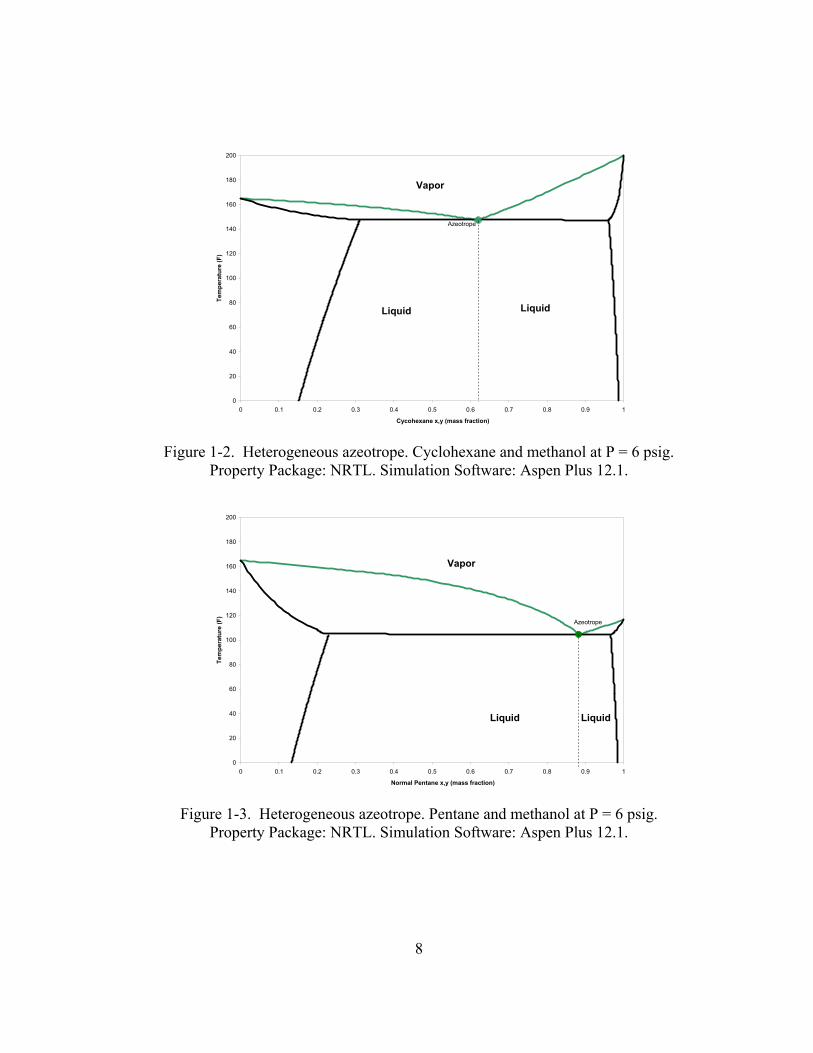
List of Figures Figure 1-1. Schematic of the relations between different fluid models [18]. .............. 4 Figure 1-2. Heterogeneous azeotrope. Cyclohexane and methanol at P = 6 psig.

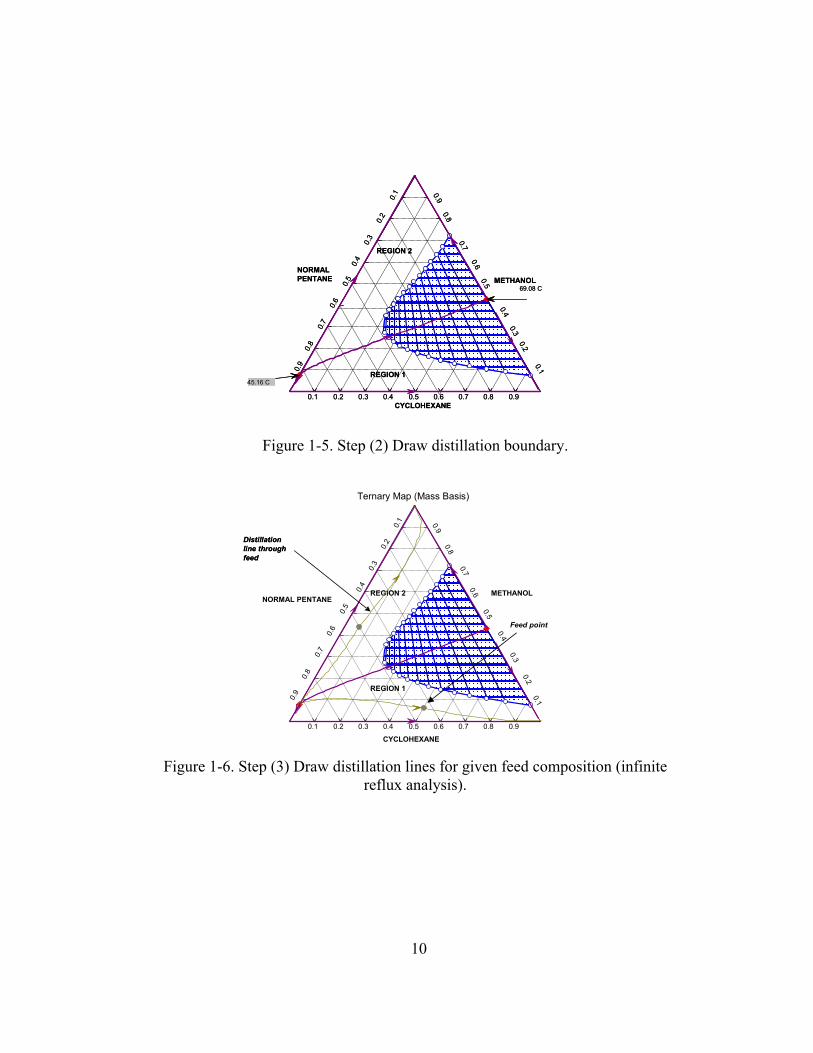
Property Package: NRTL. Simulation Software: Aspen Plus 12.1....................... 8 Figure 1-3. Heterogeneous azeotrope. Pentane and methanol at P = 6 psig.

Property Package: NRTL. Simulation Software: Aspen Plus 12.1....................... 8 Figure 1-4. Ternary map (mass basis) for cyclohexane, normal pentane and methanol.

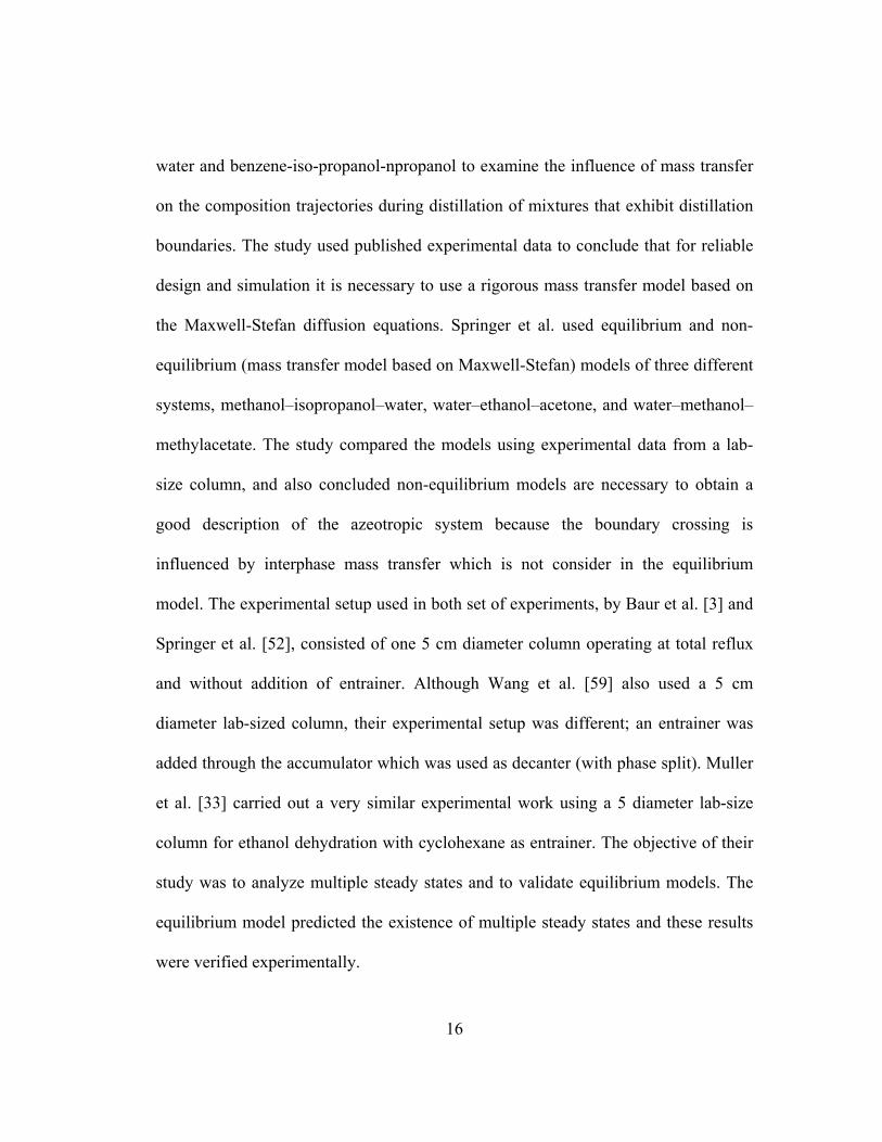
P = 6 psig. Property Package: Split from Aspen Tech........................................ 9 Figure 1-5. Step (2) Draw distillation boundary......................................................... 10 Figure 1-6. Step (3) Draw distillation lines for given feed composition (infinite reflux

analysis). ............................................................................................................. 10 Figure 1-7. Step (4) Draw feasible product areas for the given feed composition in

each distillation region. The distillate D and bottom B compositions are at the intersections of the appropriate distillation and material balance lines [19]. ..... 11

Figure 2-1. Composition control for azeotropic distillation systems [13]. ................. 21 Figure 3-1. Distillation Regions and Operating Points............................................... 26 Figure 3-2. First Distillation Region Feasible Recovery Composition Region. ......... 26 Figure 3-3. Second Distillation Region Feasible Recovery Composition Region...... 27 Figure 3-4. Picture of the column used in the experimentation.................................. 28 Figure 3-5. Process Diagram....................................................................................... 29 Figure 3-6. Column Diagram with Location of Temperature Sensors. ...................... 31 Figure 4-1. Configuration of an Equilibrium Stage. ................................................... 37 Figure 4-2. Configuration of a Non-equilibrium Segment. ........................................ 40 Figure 4-3. Equilibrium and Non-equilibrium Models Comparison with Experimental

Data for Steady State Condition #1. First Distillation Region............................ 46 Figure 4-4. Equilibrium and Non-equilibrium Models Comparison with Experimental

Data for Steady State Condition #5. First Distillation Region............................ 47 Figure 4-5. Equilibrium and Non-equilibrium Models Comparison with Experimental

Data for Steady State Condition #6. First Distillation Region............................ 48 Figure 4-6. Non-equilibrium Model Column Temperature Profile for Steady State

Condition #6........................................................................................................ 49 Figure 4-7. Experimental and Predicted Distillate Normal Pentane Composition. First

Distillation Region. ............................................................................................. 50 Figure 4-8. Column temperature profile for Steady State Condition #5..................... 52 Figure 4-9. Experimental and Predicted Distillate Normal Pentane Composition. First

Distillation Region. All models. ......................................................................... 53 Figure 4-10. Experimental and Predicted Temperature Profile Using Different

Packing Sizes in the Non-equilibrium Model..................................................... 54

xiv

Figure 4-11. Equilibrium and Non-equilibrium Models Comparison with Experimental Data. Second Distillation Region, Condition #1. ......................... 57

Figure 5-1. Dynamic Model Configuration in HYSYS.............................................. 62 Figure 5-2. Column Template used in Dynamic Model. ............................................ 63 Figure 5-3. HYSYS Dynamic Efficiency Approach................................................... 66 Figure 5-4.Simulated distillate composition response to different column efficiency

values. Distillation region one. ........................................................................... 67 Figure 5-5. Rectifying Zone Temperature Response to a Positive Step Change (90 to

110 lb/hr) in the Reflux Flow Rate. First Distillation Region. ........................... 75 Figure 5-6. Stripping Zone Temperature Response to a Positive Step Change (90 to

110 lb/hr) in the Reflux Flow Rate. First Distillation Region. ........................... 76 Figure 5-7. Simulated and Experimental Temperature Responses to a Positive Step

Change (90 to 110 lb/hr) in the Reflux Flow Rate. First Distillation Region..... 77 Figure 5-8. Composition Response to a Positive Step Change (90 to 110 lb/hr) in the

Reflux Flow Rate. First Distillation Region. ...................................................... 78 Figure 5-9. Simulation Temperature Response to a Positive Step Change (90 to 110

lb/hr) in the Reflux Flow Rate without feed composition disturbance. First Distillation Region. ............................................................................................. 80

Figure 5-10. Rectifying Zone Temperature Responses to a Negative Step Change (150-100 lb/hr) in the Reflux Flow Rate. Second Distillation Region. .............. 82

Figure 5-11. Stripping Zone Temperature Responses to a Negative Step Change (150-100 lb/hr) in the Reflux Flow Rate. Second Distillation Region. .............. 83

Figure 5-12. Simulated and Experimental Temperature Responses to a Negative Step Change (150 to100 lb/hr) in the Reflux Flow Rate. Second Distillation Region.............................................................................................................................. 84

Figure 5-13. Composition Responses to a Negative Step Change (150 to100 lb/hr) in the Reflux Flow Rate. Second Distillation Region............................................. 85

Figure 5-14. Rectifying Zone Temperature Response to a Negative Step Change (75 to 68 kBTU/hr) in the Reboiler Duty Rate. First Distillation Region................. 88

Figure 5-15. Stripping Zone Temperature Response to a Negative Step Change (75 to 68 kBTU/hr) in the Reboiler Duty Rate. First Distillation Region..................... 89

Figure 5-16. Simulated and Experimental Temperature Response to a Negative Step Change (75 to 68 kBTU/hr) in the Reboiler Duty Rate. First Distillation Region.............................................................................................................................. 90

Figure 5-17. Composition Response to a Negative Step Change (75 to 68 kBTU/hr) in the Reboiler Duty Rate. First Distillation Region........................................... 91

Figure 5-18. Rectifying Zone Temperature Responses to a Negative Step Change (106 to 61 kBTU/hr) in the Reboiler Duty Rate. Second Distillation Region. ... 93

Figure 5-19. Stripping Zone Temperature Responses to a Negative Step Change (106 to 61 kBTU/hr) in the Reboiler Duty Rate. Second Distillation Region. ........... 94

xv

Figure 5-20. Simulated and Experimental Temperature Responses to a Negative Step Change (106 to 61 kBTU/hr) in the Reboiler Duty Rate. Second Distillation Region. ................................................................................................................ 95

Figure 5-21. Composition Responses to a Negative Step Change (106 to 61 kBTU/hr) in the Reboiler Duty Rate. Second Distillation Region. ..................................... 96

Figure 5-22. Rectifying Zone Temperature Responses to a Negative Step Change (300 to 200 lb/hr) in the Feed Flow Rate. First Distillation Region. .................. 99

Figure 5-23. Stripping Zone Temperature Responses to a Negative Step Change (300 to 200 lb/hr) in the Feed Flow Rate. First Distillation Region. ........................ 100

Figure 5-24. Simulated and Experimental Temperature Responses to a Negative Step Change (300 to 200 lb/hr) in the Feed Flow Rate. First Distillation Region.... 101

Figure 5-25. Composition Response to a Negative Step Change (300 to 200 lb/hr) in the Feed Flow Rate. First Distillation Region. ................................................. 102

Figure 5-26. Rectifying Zone Temperature Responses to a Negative Step Change (300 to 200 lb/hr) in the Feed Flow Rate. Second Distillation Region............. 104

Figure 5-27. Stripping Zone Temperature Responses to a Negative Step Change (300 to 200 lb/hr) in the Feed Flow Rate. Second Distillation Region..................... 105

Figure 5-28. Simulated and Experimental Temperature Responses to a Negative Step Change (300 to 200 lb/hr) in the Feed Flow Rate. Second Distillation Region............................................................................................................................ 106

Figure 5-29. Composition Response to a Negative Step Change (300 to 200 lb/hr) in the Feed Flow Rate. Second Distillation Region. ............................................. 107

Figure 5-30. Simulated and Experimental Temperature Responses to a Step Change in Feed Composition. ............................................................................................ 109

Figure 5-31. Composition Responses to a Step Change in Feed Composition. ....... 110 Figure 6-1. a) Block diagram of a model-reference adaptive system. ...................... 115 Figure 6-2. Process Set Points Introduced to the Model........................................... 117 Figure 6-3. Model Outputs Determined by the Process Set Points........................... 119 Figure 6-4. Model Reconciliation Batch Approach.................................................. 121 Figure 6-5. Logic Diagram for Batch Reconciliation Approach. ............................. 121 Figure 6-6.Experimental Data Reconciliation. ......................................................... 122 Figure 6-7.Experimental Data Reconciliation Filtering the Heat Transfer Coefficient

Signal. ............................................................................................................... 123 Figure 6-8. Closed-loop composition control using PID controllers. Controller

response to set point changes in the distillate and bottom composition. .......... 132 Figure 6-9. PID controller response to disturbances in the feed temperature........... 132 Figure 6-10. Composition control using linear MPC................................................ 136 Figure 6-11. MPC behavior using different tuning parameters. ............................... 137 Figure 6-12. MPC closed loop response to changes in the feed temperature. PM

Tuning: Duty=25, Reflux=20. Data collected from the experiment................. 138

xvi

Figure 6-13. MPC response to unmeasured changes in the feed temperature. Data collected from the simulation............................................................................ 139

Figure 6-14. MPC response to changes in the ambient temperature. Step input. ..... 141 Figure 6-15. MPC response to changes in the ambient temperature. Ramp input.... 141 Figure 6-16. MPC response to changes in the feed composition.............................. 143

xvii

Nomenclature

Chapter 1

General Symbols

y Vapor mole fraction

x Liquid mole fraction

f Pure fluid fugacity

if̂ Fugacity of component in mixture

G Intensive Gibbs energy

n Number of moles

P Pressure

R Gas constant (8.3143 cm3MPa/moleK)

T Temperature

Greek symbols

γ Activity coefficient

ϕ Pure fluid fugacity coefficient

iϕ̂ Component fugacity coefficient in a mixture

Superscripts and subscripts

i Component in a mixture

L Liquid Phase

o Standard State

sat Saturation property

V Vapor phase

xviii

Chapter 4

General Symbols

pF Packing factor, dimension less

pdF Dry-bed packing factor, dimension less

G Gas loading, lb/hr-ft2

fG Gas loading factor

L Liquid loading, lb/hr-ft2

fL Liquid loading factor

PΔ Specific pressure drop, in.H2O/ft of packing

pbPΔ Specific pressure drop through dry bed, in.H2O/ft of packing

Greek symbols

gρ Gas density, lb/ft3

Lρ Liquid density, lb/ft3

μ Liquid viscosity, centipoise

1

Chapter 1. Introduction to Non-ideal Phase Equilibrium

Behavior and Azeotropic Distillation Systems

1.1 Introduction to Control and Dynamic Modeling of Non-ideal

Multicomponent Distillation Systems

Industrial production of chemicals involves purification and recovery of the

products, by-products and unreacted raw materials. Distillation is clearly the

dominant separation process, and the largest energy consumer. Improving its process

efficiency is an on-going goal of the chemical processing and refining industries.

In recent years, the use of dynamic modeling in chemical and refining

applications has been intensified with the adoption of commercial process modeling

software and increasing computer processing capabilities. The models are used in a

broad range of applications like parameter estimation, process optimization, and

control. Most modern control methods require some kind of process model to predict

future process outputs but industrial applications do not currently link high fidelity

dynamic models developed in commercial software with the control software.

Some model-based control and optimization techniques are based on adaptive

steady state models that account for the physical drifting of the process itself (such as

fouling of a heat exchanger, temperature fluctuation of the feed, etc.) or changes in

2

market demands and economic conditions, which may result in change of product

specifications and plant schedules.

The approach presented in this work links the process high fidelity dynamic

model with the control software used in the process. The model is modified online

using a feedback configuration to eliminate the difference between the process and

model outputs. The high fidelity model is used in the implementation of control

strategies and to infer process parameters that cannot be determined with field

instrumentation. The high fidelity model is developed following a methodology that

includes five steps: (1) the system physical and thermodynamic behavior is analyzed;

(2) different modeling approaches are studied and compared with process data to

determine the most suitable method to model the system; (3) the model is developed

and validated with process data; (4) the model parameters that will be updated on-line

are selected; and (5) the model updating method is implemented.

1.2 Azeotropy

Common non-ideal liquid mixtures are generated by mixing polar and non-

polar components, often resulting in the formation of azeotropes. Binary azeotropic

mixtures may often be effectively separated by distillation by adding a liquid material

(solvent or entrainer) to the system which results in a ternary mixture. Ternary

systems are studied by using ternary plots; such an analysis helps design engineers to

visualize the separation possibilities and constraints.

3

An azeotrope is a liquid mixture of two or more components that has a unique

constant boiling point. This boiling point may be higher or lower than the boiling

points of the mixture components. Since the liquid retains the same composition as it

is boiled, the vapor has the same composition as the liquid and simple distillation will

not separate the components. An azeotrope is said to be positive if the constant

boiling point is at a temperature maximum and negative when the boiling point is at a

temperature minimum. There are two types of azeotropes: homogeneous azeotropes,

where only one liquid phase coexists with the vapor phase, and heterogeneous

azeotropes, where two liquid phases coexist with the vapor phase. Systems with more

than one azeotrope are highly non-ideal and involve distillation challenges like the

presence of distillation boundaries and two or more liquid phase formations.

Although separation of highly non-ideal multicomponent mixtures is a

common practice in chemical industries, very few published experimental studies

have utilized dynamic modeling and control of such systems.

1.2.1 Phase Equilibrium, non-ideality and azeotropy

Based on a Venn diagram, Figure 1-1 illustrates the modeling of phase

equilibrium.

4

Figure 1-1. Schematic of the relations between different fluid models [18].

In the model, the vapor is represented by an equation of state while the liquid is represented by the activity coefficient model.

The pressure, temperature and volume relations of the vapor phase are

normally represented with equation of state (EOS) models. The simplest EOS model

is the ideal gas law, which is relatively accurate for gases at low pressures and high

temperatures. Since this equation becomes increasingly inaccurate at higher pressures

and lower temperatures, a number of much more accurate equations of state have

been developed.

In this work, The Redlich-Kwong Equation of State was used to calculate the

vapor phase fugacity. This model was published in 1949 by Redlich and Kwong [40].

A summary of the model is given in Equation (1-1).

)(5.0 bVVTa

bVRTp

+−

−= (1-1)

Ideal Gas Model

Pyf iv

i =ˆIdeal Solution Model

Pyf iv

iv

i ϕ=ˆ

oiii fxf =ˆ

1=iγ

1ˆ ≠iϕ

ii ϕϕ ≠ˆ

Pyf iii ϕ̂ˆ =Departure Functions

Non-ideal Solution Model

oiiii fxf γ=ˆ 1≠iγ

ii ϕϕ =ˆ

ijnPTi

E

i nGRT

≠

⎥⎦

⎤⎢⎣

⎡∂

∂=

,,

lnγ

Excess Properties

Modified Raoult’s Law

satiii

Li Pxf γ≈ˆ

5

where the parameters a and b can be determined with the data of the critical point

(Equation (1-2)).

c

c

c

c

pTR

pTRa

5.225.22

31

4275.0129

1=

⎟⎟⎠

⎞⎜⎜⎝

⎛−

= ; c

c

c

c

pRT

pRTb 08664.0

312 3

1

=−

=

(1-2)

Non-ideal liquids are modeled using activity coefficient models. At low to

moderate pressures and temperatures away from the critical point, the vapor-liquid

phase equilibrium for a multicomponent mixture is given by equation (1-3).

)(),( TPxTxPy satiiii γ= ; i = 1, 2 … n (1-3)

where yi and xi are the mole fractions of species i in the vapor and liquid phases,

respectively, γi is the activity coefficient of species i in the liquid phase, satiP is the

saturated vapor pressure of species i at temperature T, and P is the system pressure.

The activity coefficient γ is a measure of the non-ideality of a mixture and depends on

temperature and composition. When γ = 1, the mixture is said to be ideal and

equation (1-3) simplifies to Raoult’s law (equation (1-4)).

)(TPxPy satiii = ; i = 1, 2 … n (1-4)

Solutions containing dissimilar polar species usually exhibit positive (γ > 1)

or negative (γ < 1) deviations from Raoult’s law. If these deviations become so large

that the vapor pressure exhibits an extreme point at constant temperature, or,

6

equivalently, an extreme point in the boiling temperature at constant pressure, the

mixture is azeotropic.

The activity coefficient is obtained after models of the excess Gibbs energy

normally based on experimental data. The liquid phase models used in this work were

based on the NRTL (nonrandom, two-liquid) equation of Renon and Prausnitz [38].

The model for multicomponent systems as well as the parameters used in this work

are summarized in the Appendix.

1.2.2 Graphical Tools for Analysis of Phase Equilibrium Behavior

The equilibrium compositions of the liquid and vapor phase in a mixture are a

function of the mixtures temperature and pressure. The equilibrium condition is

represented by equation (1-5).

),,( xPTfy = (1-5)

P and T represent the mixture pressure and temperature while y and x represent the

vapor and liquid compositions. In addition to the condition established by equation

(1-5), at the equilibrium state the sum of all composition fractions in each phase must

equal to unity; this condition is represented by equation (1-6) .

1=∑n

iiy , 1=∑

n

iix (1-6)

Equilibrium conditions are graphically represented by diagrams where one of

the variables is fixed (isobaric or isothermal conditions) and an equilibrium mapping

7

function assigns a composition in the liquid phase to the corresponding equilibrium

vapor phase composition.

The possibility to graphically represent a system’s vapor-liquid equilibrium

depends on the number of components in the mixture. In a mixture of n components,

the composition space is (n-1)-dimensional because the sum of mole fractions must

be equal to unity.

1.2.3 Binary and Ternary Diagrams for Normal Pentane, Methanol and

Cyclohexane

The system selected for this research was a ternary mixture of methanol,

normal pentane and cyclohexane. The mixture’s binary phase diagrams are presented

in Figure 1-2 for cyclohexane and methanol, and Figure 1-3 for normal pentane and

methanol.

The non-ideal behavior of the binary mixtures with methanol can be seen from

the diagrams. Methanol forms two heterogeneous azeotropes, one with cyclohexane

and one with pentane. Heterogeneous azeotropes are usually present when positive

deviations from Raoult’s Law are sufficiently large, with γ values typically greater

than four, Equation (1-3). The two liquid phases in the heterogeneous azeotropic

point have different compositions but the overall composition is equal to the

composition of the vapor phase. This thermodynamic behavior can also be studied

with ternary diagrams.

8

0

20

40

60

80

100

120

140

160

180

200

0 0.1 0.2 0.3 0.4 0.5 0.6 0.7 0.8 0.9 1

Cycohexane x,y (mass fraction)

Tem

pera

ture

(F)

Azeotrope

Liquid

Vapor

Liquid

Figure 1-2. Heterogeneous azeotrope. Cyclohexane and methanol at P = 6 psig.

Property Package: NRTL. Simulation Software: Aspen Plus 12.1.

0

20

40

60

80

100

120

140

160

180

200

0 0.1 0.2 0.3 0.4 0.5 0.6 0.7 0.8 0.9 1

Normal Pentane x,y (mass fraction)

Tem

pera

ture

(F)

Azeotrope

Liquid

Vapor

Liquid

Figure 1-3. Heterogeneous azeotrope. Pentane and methanol at P = 6 psig.

Property Package: NRTL. Simulation Software: Aspen Plus 12.1.

9

The mixture’s ternary diagram is presented in Figure 1-4 where both

azeotropes can be appreciated. The two azeotropes divide the diagram into two

distillation regions. Figures 1-4 to 1-7 illustrate step by step how to determine the

feasible product region using ternary diagrams. First draw the ternary diagram and

locate the two system’s azeotropes in the map. Then, draw the distillation boundary

by connecting the two azeotropic points. Continue drawing the distillation line for the

given feed composition and finally, determine the feasible product areas using the

intersections between the distillation and material balances lines.

CYCLOHEXANE

METHANOL

0.1 0.2 0.3 0.4 0.5 0.6 0.7 0.8 0.9

0.1

0.2

0.3

0.40.5

0.6

0.7

0.8

0.9

0.9

0.8

0.7

0.6

0.5

0.4

0.3

0.2

0.1

69.08 C

45.16 C

NORMAL PENTANE

C5 – MeOHAzeotrope92% C58% MeOH

C6 – MeOHAzeotrope64% C646% MeOH

Two Liquid phases

Figure 1-4. Ternary map (mass basis) for cyclohexane, normal pentane and

methanol. P = 6 psig. Property Package: Split from Aspen Tech. Step (1) Locate all system’s azeotropes in the map.

10

CYCLOHEXANE

NORMAL PENTANE METHANOL

0.1 0.2 0.3 0.4 0.5 0.6 0.7 0.8 0.9

0.1

0.2

0.3

0.4

0.5

0.6

0.7

0.8

0.9

0.9

0.8

0.7

0.6

0.5

0.4

0.3

0.2

0.1

69.08 C

45.16 CREGION 1

REGION 2

CYCLOHEXANE


0.1 0.2 0.3 0.4 0.5 0.6 0.7 0.8 0.9

0.1

0.2

0.3

0.4

0.5

0.6

0.7

0.8

0.9

0.9

0.8

0.7

0.6

0.5

0.4

0.3

0.2

0.1

69.08 C

45.16 CREGION 1

REGION 2

Figure 1-5. Step (2) Draw distillation boundary.

Ternary Map (Mass Basis)

CYCLOHEXANE

NORMAL PENTANEMETHANOL

0.1 0.2 0.3 0.4 0.5 0.6 0.7 0.8 0.9

0.1

0.2

0.3

0.4

0.5

0.6

0.7

0.8

0.9

0.9

0.8

0.7

0.6

0.5

0.4

0.3

0.2

0.1

REGION 1

REGION 2

Feed point

Distillation line through feed

Distillation line through feed

Figure 1-6. Step (3) Draw distillation lines for given feed composition (infinite

reflux analysis).

11

CYCLOHEXANE


0.1 0.2 0.3 0.4 0.5 0.6 0.7 0.8 0.9

0.1

0.2

0.30.4

0.50.6

0.7

0.8

0.9

0.9

0.8

0.7

0.6

0.5

0.4

0.3

0.2

0.1

69.08 C

45.16 CREGION 1

REGION 2

B

D

BD

Material balance linesdirect splitindirect split

F

F

Figure 1-7. Step (4) Draw feasible product areas for the given feed composition in

each distillation region. The distillate D and bottom B compositions are at the intersections of the appropriate distillation and material balance lines [19].

1.3 Understanding Azeotropic Distillation

Azeotropic distillation is a process widely used to separate non-ideal binary

mixtures. This separation technique uses another component; known as an entrainer.

Depending on the mixture, the entrainer forms an azeotrope with one of the

components in the binary mixture or breaks an existing azeotrope in the binary

mixture. There are three types of azeotropic distillation: homogeneous azeotropic

distillation, heterogeneous azeotropic distillation and extractive distillation.

Homogeneous azeotropic distillation uses the entrainer to form a

homogeneous azeotrope with one of the feed components. The entrainer can be added

at the top or bottom of the column depending on whether the azeotrope is recovered

12

at the top or bottom of the column. Heterogeneous azeotropic distillation uses the

entrainer to form a heterogeneous azeotrope in the reflux drum which is also used as

decanter. One of the liquid phases is recovered as product and the other is sent back

as reflux to the column. The entrainer is usually called the “solvent” when referring to

extractive distillation. This separation process uses a large amount of a relative high-

boiling solvent to alter the liquid-phase activity coefficient of the binary mixture and

break an azeotrope. The solvent is added above the feed entry and a few trays below

the top.

Azeotropic distillation presents multiple challenges in design and operation

due to the presence of non-idealities, phase splitting, possible multiple steady states,

and distillation boundaries. When designing these systems it is important to keep in

mind that boundaries cannot be crossed. For these reason, in order to isolate two pure

components which lie in two different distillation regions, it is necessary to have two

different feed compositions (one from each of the two regions) and two distillation

columns [15].

1.4 Dissertation Outline

Chapter 2 reviews the current status of modeling and control of non-ideal

multicomponent distillation systems emphasizing azeotropic distillation. Chapter 3

describes the experimental system including the system properties, process

configuration, and detailed equipment description. Chapter 4 explains the

13

methodology used to develop steady state models for azeotropic distillation and

compares the results when implementing the model with the equilibrium and non-

equilibrium approach. Chapter 5 presents dynamic process data from the process

described in the previous chapter and the dynamic model developed based on that

data. Chapter 6 describes the model reconciliation module and the results after its

online implementation in the process. Chapter 6 also introduces a control study for

azeotropic distillation where different control approaches are implemented in the

process. Finally Chapter 7 summarizes the results presented and proposes future

extensions of this research.

14

Chapter 2. Status of Modeling and Control of Azeotropic

Distillation

2.1 Dynamic Modeling of Azeotropic Distillation Columns

Modeling, design and operation of distillation systems have been extensively

studied by industry and academy during the past years, establishing distillation as the

most mature separation operation [46]. Different algorithms for solving equilibrium

models were widely published from the late 1950s to the early 1990s [45] until the

development of the non-equilibrium model was introduced by Krishna and Taylor in

the late 1980s [23], [24], [25], [55], which models the mass transfer-rate across

distillation and adsorption columns using the Maxwell-Stefan equations. Due to its

complexity, non-equilibrium or rate-based model solutions require more CPU time

than the solutions of the equilibrium models.

Most of published dynamic models on non-ideal multicomponent distillation

separations are related to heterogeneous azeotropic distillation. This process is the

most widely used to separate azeotropic mixtures with low relative volatilities.

Heterogeneous azeotropic distillation uses a third component (entrainer) to form a

heterogeneous azeotrope in the reflux drum. One of the phases is recovered as

product and the other is sent back as reflux to the column. Although the reflux drum

15

is used as a decanter, this process usually requires more than one column to recover

the entrainer.

Chien et al. [12], [14] compared two different models where two and three

columns were used to separate a mixture of isopropyl alcohol + water with

cyclohexane as entrainer. The studied concluded that optimum design of the two

column approach is more economical than the three column approach. Kurooka et al.

[27] developed a dynamic simulator to characterize a distillation column for the

separation of water, n-butyl-acetate and acetic acid. The system used in this study

displayed a complex dynamic behavior, increasing the operation and control

challenges. The dynamic model was used to investigate the performance of a

nonlinear controller with exact input-output linearization of a simplified model.

Although dynamic simulation was developed for these works, no experimental data

was presented to validate the models.

Wang et al. [59] performed experimental validations of dynamic and steady

state models for the mixture of isopropyl alcohol + water with cyclohexane as

entrainer where the objective was the analysis of multiple steady states, parametric

sensitivity and critical reflux. The study used a laboratory scale, 5 cm diameter, sieve

plate distillation column. Baur et al. [3] and Springer et al. [52] also carried out

experiments for model validation using a lab-size column, similar to the one used in

the parametric sensitivity research, but studied multicomponent diffusion and

multiphase hydrodynamics. Baur et al. used two systems, methanol-iso-propanol-

16

water and benzene-iso-propanol-npropanol to examine the influence of mass transfer

on the composition trajectories during distillation of mixtures that exhibit distillation

boundaries. The study used published experimental data to conclude that for reliable

design and simulation it is necessary to use a rigorous mass transfer model based on

the Maxwell-Stefan diffusion equations. Springer et al. used equilibrium and non-

equilibrium (mass transfer model based on Maxwell-Stefan) models of three different

systems, methanol–isopropanol–water, water–ethanol–acetone, and water–methanol–

methylacetate. The study compared the models using experimental data from a lab-

size column, and also concluded non-equilibrium models are necessary to obtain a

good description of the azeotropic system because the boundary crossing is

influenced by interphase mass transfer which is not consider in the equilibrium

model. The experimental setup used in both set of experiments, by Baur et al. [3] and

Springer et al. [52], consisted of one 5 cm diameter column operating at total reflux

and without addition of entrainer. Although Wang et al. [59] also used a 5 cm

diameter lab-sized column, their experimental setup was different; an entrainer was

added through the accumulator which was used as decanter (with phase split). Muller

et al. [33] carried out a very similar experimental work using a 5 diameter lab-size

column for ethanol dehydration with cyclohexane as entrainer. The objective of their

study was to analyze multiple steady states and to validate equilibrium models. The

equilibrium model predicted the existence of multiple steady states and these results

were verified experimentally.

17

Yamamoto et al. [64] presented an industrial example of heterogeneous

azeotropic distillation of acetic acid + water with n-butyl-acetate as an entrainer. This

work investigated the column behavior by using dynamic simulation and developed a

control system tested in the industrial application. The control performance was

presented but the publication omitted experimental data and information on dynamic

model validation.

Repke et al. [41] developed a non-equilibrium steady state model for the

separation of a three phase system in a packed distillation column and validated the

results with experimental data. The study used a 7 cm diameter column, of 7.5 m

height with effective packing height of 2.5m and investigated various heterogeneous

mixtures, such as acetone/toluene/water and 1-propanol/1-butanol/water. The

system’s behavior was better described by the non-equilibrium model than the

equilibrium model, which at some conditions failed to predict the experimental

behavior.

Another variation of azeotropic distillation is homogeneous azeotropic

distillation. As in heterogeneous azeotropic distillation, homogeneous azeotropic

distillation also uses an entrainer, which forms a homogeneous azeotrope with one of

the feed components. It is added to the top or bottom of the column depending on

whether the azeotrope is recover at the top or bottom of the column. In homogeneous

azeotropic distillation a single liquid phase is in equilibrium with the vapor phase,

18

while in heterogeneous azeotropic distillation the overall liquid composition, which

forms two liquid phases, is identical to the vapor composition.

Extractive distillation is another technique used to separate azeotropic mixtures.

It uses a large amount of a relative high-boiling solvent to alter the liquid-phase

activity coefficient of a binary mixture and break the azeotrope. The solvent is added

above the feed entry point, a few trays below the top. Maciel and Brito [30] evaluated

the dynamic behavior of an extractive distillation column for the dehydration of

aqueous ethanol mixture using ethylene glycol as solvent. Using theoretical modeling

and computer simulation, the authors concluded production was highly sensitive to

feed composition disturbances and pointed the necessity of utilization of advanced

control strategies. Kumar et al. [26] developed steady state and dynamic mass and

energy balance models for an extractive tray distillation column separating acetone

and methanol using water as solvent. The literature data used in the study was

obtained in a 15 cm diameter, 2 m height tray column. The models were fitted to the

experimental data modifying the Murphree tray efficiencies. The column presented

nonlinear behavior illustrated by gain changes at different operating conditions. The

study also reported highly non-ideal column profiles and highlighted the importance

of good simulations for nonlinear multicomponent systems.

19

2.2 Control of Azeotropic Distillation Columns

The characteristics of highly non-ideal mixtures present a challenge for process

control. Several studies can be found in the literature addressing the multicomponent

distillation control problem [11]. In general the main objective of distillation control

is to maintain a desired product quality, however, direct composition control is

complicated by the fact that on-line composition analyzers are expensive and difficult

to maintain. This problem has typically been addressed using temperature

measurements in the column in an inferential control strategy. Luyben and Vinante

[29] recommend the use of multiple temperature measurements instead of the

traditional approach based on just one optimal tray temperature measurement. Weber

and Mosler [61] at Esso Research and Engineering patented a multiple temperature

controller to maintain the columns product composition. Brosilow and co-workers

[20], [35] developed an inferential control technique using more variables than just

temperature to infer composition. Patke and Deshpande [36] did an experimental

study in a laboratory scale distillation column to compare the different approaches of

temperature control and inferential control and recommended inferential control over

the temperature control scheme. Yu and Luyben [65] designed a composition control

system by using several temperature measurements in multicomponent distillation

and recommended this approach over the traditional single temperature control and

the inferential control scheme. More recently, Luyben [28] presented a methodology

20

for the selection of effective control structures for ternary distillation columns using

only temperature measurements.

Multivariable distillation control research has also been focused in the choice

and analysis of different control structures. Among others, Skogestad and Morari [48]

extensively studied the subject using the Relative Gain Array (RGA) method [32],

[49], [50], [51], [63]. The RGA steady state analysis, initially introduced by Bristol

[9], has found widespread use in the industry.

In previous control studies for azeotropic distillation systems, overhead

configurations varied within the studies. In general two liquid phases formed in the

entrainer, and one of them was usually put back in the column as reflux and the other

recovered as distillate product. Another difference between the traditional and the

azeotropic distillation process configurations is an additional feed input in the

overhead accumulator to make up for material imbalance and to respond to

disturbances.

Chien et al. [13] constructed a laboratory scale sieve distillation column for

the separation of water + 2-propanol using cyclohexane as an entrainer to test

different traditional control approaches, and concluded that a non-traditional inverse

double loop temperature control scheme was necessary to maintain the desired

temperature profile. This approach is different from the traditional approach in the

sense that the top temperature is paired with reboiler duty while bottom temperature

is paired with reflux flow rate (Figure 2-1). Tonelli et al. [57] studied the same system

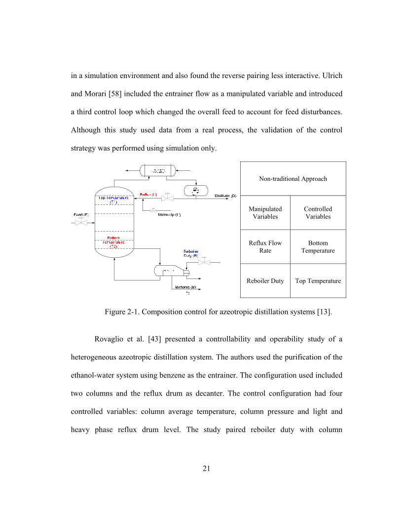
21

in a simulation environment and also found the reverse pairing less interactive. Ulrich

and Morari [58] included the entrainer flow as a manipulated variable and introduced

a third control loop which changed the overall feed to account for feed disturbances.

Although this study used data from a real process, the validation of the control

strategy was performed using simulation only.

Non-traditional Approach

Manipulated Variables

Controlled Variables

Reflux Flow Rate

Bottom Temperature

Reboiler Duty Top Temperature

Figure 2-1. Composition control for azeotropic distillation systems [13].

Rovaglio et al. [43] presented a controllability and operability study of a

heterogeneous azeotropic distillation system. The authors used the purification of the

ethanol-water system using benzene as the entrainer. The configuration used included

two columns and the reflux drum as decanter. The control configuration had four

controlled variables: column average temperature, column pressure and light and

heavy phase reflux drum level. The study paired reboiler duty with column

22

temperature and reflux flow rate with reflux drum level. Column pressure was paired

with overhead vapor flow rate. Controllability studies comparing the use of one and

two columns including more variables and common approaches used in this kind of

process are needed.

2.3 Ternary Diagrams and Multiple Steady States

Widagdo and Seider [62] surveyed results from the literature on the use of

theoretical models and computer simulation. They found that azeotropic distillation

(homogeneous and heterogeneous) displayed highly nonlinear behavior indicated by

presence of multiple steady states. An important conclusion from this review was the

necessity of clarifying the sources of the multiple steady states and showing their

presence experimentally. The survey also acknowledged the application of complex

graphical constructions as a basic tool for the design of separation systems of high

non-ideal mixtures. In their work, the authors examined maps of residue curves,

distillation lines, and geometric methods for design, analysis of dynamic and steady

state behavior, and control of azeotropic systems. More recently, De Villiers et al.

[17] presented a review on the use of residue curve maps to analyze phase

equilibrium data predicted from thermodynamic packages and Kiva et al. presented a

survey in azeotropic phase equilibrium diagrams comprising less-known published

results mainly from Russian literature [22].

23

Graphical analysis of ternary systems is possible by commercial process

simulation software such as DISTIL from Aspentech and CHEMCAD from

Chemstations. A residue curve represents the residue composition of a simple batch

distillation column, while a distillation line represents the operation line of a

distillation column at total reflux.

Multiple steady states presented in azeotropic ternary systems can be detected

by graphical analysis using residue curve maps. Residue curve analysis shows the

different paths connecting given compositions in a ternary distillation column helping

to identify different operating conditions given to the same inputs and column

configuration. Several publications have been reported trying to explain the nature of

the phenomena.

Wang et al. [60] studied an azeotropic distillation system of isopropyl alcohol,

cyclohexane and water and showed that there are two paths connecting a high purity

isopropyl alcohol product and the ternary azeotrope distillate. The path was

determined by the reflux rate operating condition. The study was validated with

experimental results.

A detailed study of multiple steady states for homogeneous and heterogeneous

azeotropic distillation was presented by Bekiaris et al. [4], [5], [6]. They showed the

existence of multiple steady states for both systems and derived a necessary and

sufficient condition for the existence of these multiple steady states based on the

geometry of the distillation region boundaries and product paths.

24

Chapter 3. Experimental System Description

This chapter describes the system and equipment used in the experimental

part of the project. The plant where the experiments were carried out belongs to the

Separation Research Program, which is located in the Pickle Research Campus, a

research facility of the University of Texas at Austin.

3.1 Process Description

The chemical system selected for the experiments performed in this research

was a ternary mixture of cyclohexane, normal pentane and methanol. The

thermodynamic behavior of the mixture as well as its binary and ternary plots were

presented in section 1.2.3.

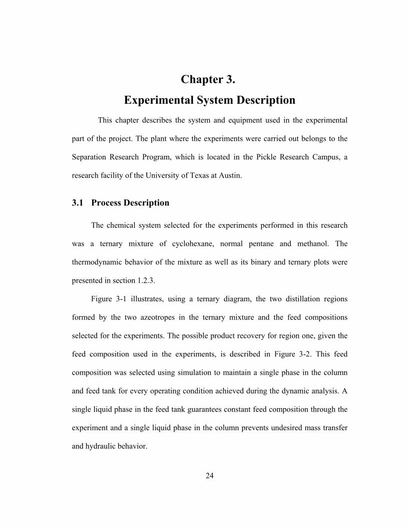
Figure 3-1 illustrates, using a ternary diagram, the two distillation regions

formed by the two azeotropes in the ternary mixture and the feed compositions

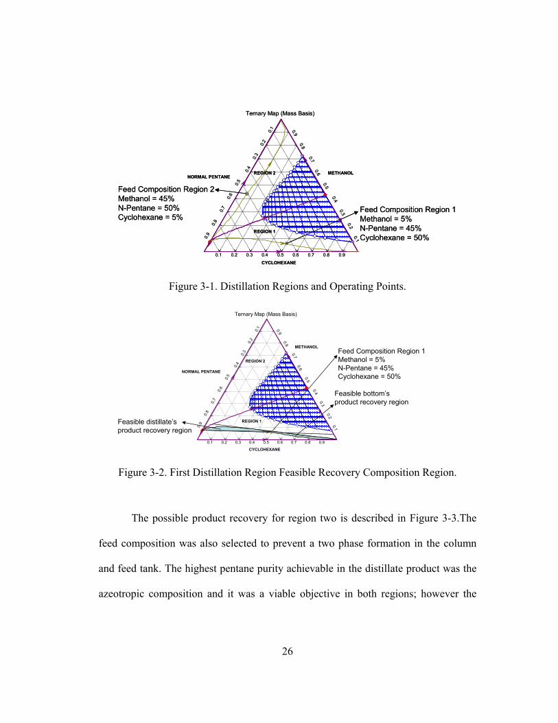
selected for the experiments. The possible product recovery for region one, given the

feed composition used in the experiments, is described in Figure 3-2. This feed

composition was selected using simulation to maintain a single phase in the column

and feed tank for every operating condition achieved during the dynamic analysis. A

single liquid phase in the feed tank guarantees constant feed composition through the

experiment and a single liquid phase in the column prevents undesired mass transfer

and hydraulic behavior.

25

Table 3-1. System properties1.

Methanol Normal Pentane Cyclohexane

Formula CH4O C5H12 C6H12

Molecular Weight 32.04190063 72.151 84.16

Molar Density [kgmole/m3] 24.531987 8.603021 9.189436

Mass Density [kg/m3] 786.0514899 620.7165 773.383

Mass Enthalpy [kcal/kg] -1785.97602 -572.454 -441.892

Mass Entropy [kJ/kg-C] 0.264072486 1.010161 -2.40188

Heat Capacity [kJ/kgmole-C] 115.4849955 167.7808 149.5317

Mass Heat Capacity [kJ/kg-C] 3.604186804 2.325413 1.776755

Antoine’s coefficients: fTeTdcT

baP *)ln(*)ln( +++

+= , kPaP = , )(KT

A 0 63.198 70.9775

B 0.6602 -1.17E-02 -6187.1

C 1.11E-03 3.32E-03 0

D 2.69E-07 -1.17E-06 -8.46523

E -2.23E-10 2.00E-10 6.45E-06

F 0 -8.66E-15 0

1 Source: HYSYS thermodynamic library. The vapor enthalpy equation is integrated by Hysys to calculate entropy. This calculation is performed on mass basis with the reference point being an ideal gas at 0 K.

26


CYCLOHEXANE


0.1 0.2 0.3 0.4 0.5 0.6 0.7 0.8 0.9

0.1

0.2

0.3

0.4

0.5

0.6

0.7

0.8

0.9

0.9

0.8

0.7

0.6

0.5

0.4

0.3

0.2

0.1

REGION 1

REGION 2

Feed Composition Region 1Methanol = 5%N-Pentane = 45%Cyclohexane = 50%



CYCLOHEXANE


0.1 0.2 0.3 0.4 0.5 0.6 0.7 0.8 0.9

0.1

0.2

0.3

0.4

0.5

0.6

0.7

0.8

0.9

0.9

0.8

0.7

0.6

0.5

0.4

0.3

0.2

0.1

REGION 1

REGION 2



Figure 3-1. Distillation Regions and Operating Points.


CYCLOHEXANE

NORMAL PENTANE

METHANOL

0.1 0.2 0.3 0.4 0.5 0.6 0.7 0.8 0.9

0.1

0.2

0.3

0.4

0.5

0.6

0.7

0.8

0.9

0.9

0.8

0.7

0.6

0.5

0.4

0.3

0.2

0.1

REGION 1

REGION 2


Feasible bottom’s product recovery region

Feasible distillate’s product recovery region

Figure 3-2. First Distillation Region Feasible Recovery Composition Region.

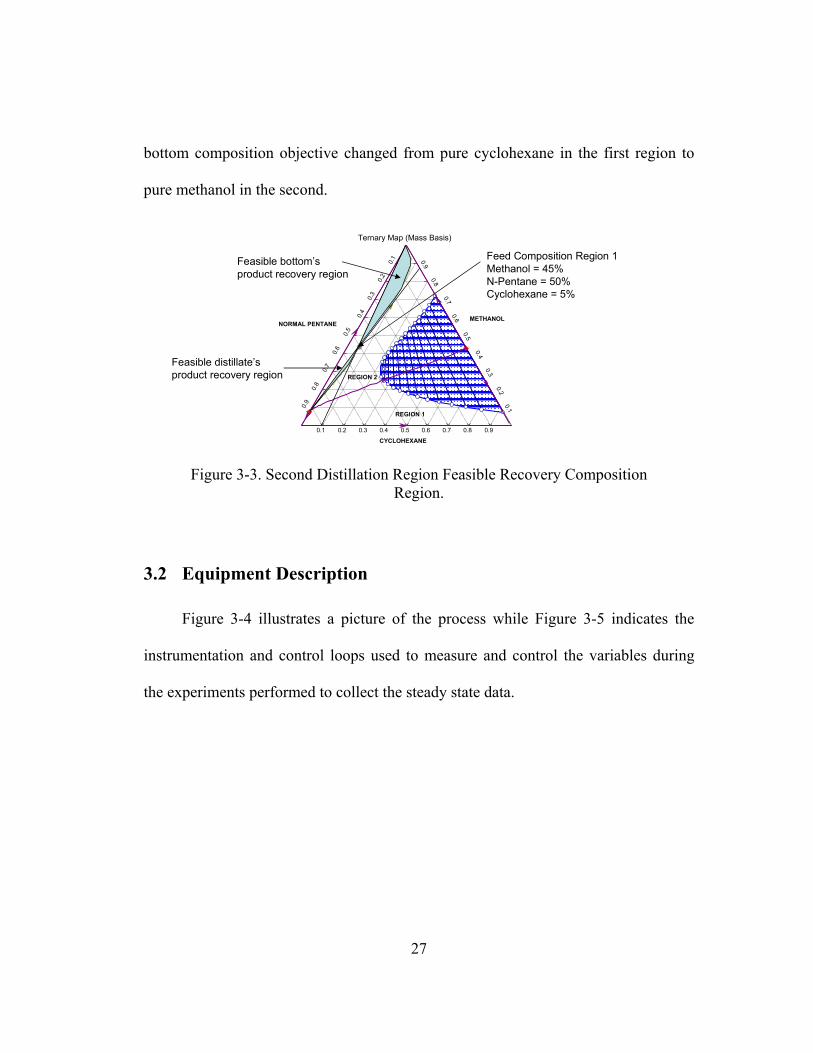
The possible product recovery for region two is described in Figure 3-3.The

feed composition was also selected to prevent a two phase formation in the column

and feed tank. The highest pentane purity achievable in the distillate product was the

azeotropic composition and it was a viable objective in both regions; however the

27

bottom composition objective changed from pure cyclohexane in the first region to

pure methanol in the second.


CYCLOHEXANE


0.1 0.2 0.3 0.4 0.5 0.6 0.7 0.8 0.9

0.1

0.2

0.3

0.4

0.5

0.6

0.7

0.8

0.9

0.9

0.8

0.7

0.6

0.5

0.4

0.3

0.2

0.1

REGION 1

REGION 2


Feasible bottom’s product recovery region

Feasible distillate’s product recovery region

Figure 3-3. Second Distillation Region Feasible Recovery Composition Region.

3.2 Equipment Description

Figure 3-4 illustrates a picture of the process while Figure 3-5 indicates the

instrumentation and control loops used to measure and control the variables during

the experiments performed to collect the steady state data.

28

Figure 3-4. Picture of the column used in the experimentation.

29

Figure 3-5. Process Diagram.

30

3.2.1 Vessels

3.2.1.1 Feed tank

Dimensions: 2.5 ft diameter x 3 ft.

Total volume = 110 gal.

Volume charged = 91 gal.

Hold-up during operation = 40 gal.

3.2.1.2 Column (Figure 3-6)

Dimensions: 6 in diameter x 34.75 ft.

Internal Type: Packed (No. 0.7 Nutter Ring Metal Random)

Packed Height: 30 ft.

3.2.1.3 Accumulator

Dimensions: 8 in diameter x 3 ft.

Total volume: 7.8gal.

Hold-up during operation: 5 gal.

3.2.2 Heat Exchangers

3.2.2.1 Reboiler

Type = Horizontal kettle reboiler with liquid overfow

Heat Transfer surface area = 78.4 sqft.

Configuration – 1 shell pass, 1 tube pass.

31

Tube side – condensing steam

Shell side – boiling process stream

Figure 3-6. Column Diagram with Location of Temperature Sensors.

3.2.2.2 Condenser

Type = Tube and shell heat exchanger.

Tube side - Cooling water

Cooling water flow = 5 gpm

Exit temperature for cold water = 58.5 F

Shell Side – Condensing vapor

Orientation = horizontal

34.75 ft 30 ft

7.7 ft

Feed Point

2 ft TT-6071

5.5 ftTT-6072

2 ft TT-6073 2 ft TT-6074 2.83 ft TT-6075

2 ft TT-6076 2 ft TT-6077 2 ft TT-6078 1 ft TT-6079

32

Heat Transfer surface area = 34 sqft

1-pass flow (shell and tube side)

3.2.3 Instrumentation

The process sensors, actuators and controllers were provided by Emerson

Process Management, as described below.

3.2.3.1 Temperature sensors

The process has twenty-four temperature sensors connected to four

Rosemount 848T’s eight-input temperature transmitters with a Foundation Fieldbus

segment. Nine temperature sensors are located in the column (Figure 3-6), and the

others are located in the different process streams.

3.2.3.2 Level sensors

There are four level measurements in the process located in the feed tank,

accumulator, reboiler and bottom of the column. The hold-up in the bottom of the

column is measured with a Rosemount 1151 pressure transmitter with Foundation

Fieldbus.

3.2.3.3 Flow sensors

The process has four Micromotion coriolis flow meters to measure feed,

reflux, distillate, and bottom flow rate. These sensors are equipped with HART

33

communication devices. In addition to the Micromotion meter, there are three orifice

flow meters in the utility lines (cold water, reboiler, and preheater steam).

3.2.3.4 Pressure sensors

In addition to the steam pressure sensors, there are two sensors to measure

pressure in the condenser and the differential column pressure.

3.2.3.5 Control valves

There are four Fisher control valves associated with the same streams as the

Micromotion flow meters and two others associated with the reboiler and preheater

steam line.

3.2.3.6 Control system

The experimental plant is operated through a DeltaV control system from

Emerson Process Management. The DeltaV system includes three workstations, a

control network, two controllers (second is redundant) and an I/O subsystem. The

work stations provide a graphical user interface to the process and system

configuration functions. The three work stations communicate among themselves and

two controllers by a control network. The primary controller performs control and

manages communications between the I/O subsystem and the control network. The

I/O subsystem processes information to and from field devices.

34

Chapter 4. Steady State Models for Azeotropic Distillation In order to determine whether or not equilibrium models could be used to

accurately predict the azeotropic system behavior, a non-equilibrium steady state

model was developed, and its results were compared with an equilibrium model. Both

models used the same equipment configuration, operating conditions, and

thermodynamic properties. Conditions from the two distillation regions were

simulated, and their results were validated experimentally. The two steady state

models presented in this chapter were developed using Aspen Technology software.

Equilibrium models were developed in HYSYS and Aspen Plus, and one rate-based

or non-equilibrium model was developed in Aspen Plus.

4.1 Model Configuration

The column configuration is summarized in Table 4-1. The activity

coefficient model NRTL was used as the main property method for the liquid phase

while the Redlich-Kwong equation-of-state was used for the calculations in the gas

phase. The thermodynamic models were described in previous chapters and the

Appendix.

35

Table 4-1. Column Configuration for Steady State Simulation.

Number of Theoretical Stages 24 (Without condenser and reboiler) Feed Stage 18 Condenser Type Total (Stage 1) Reboiler Type KETTLE (Stage 26) Valid Phases Vapor-Liquid-Liquid Internal Type Packed (Nutter Ring Metal Random No. 0.7)Stage Packing Height [in] 13.84615 Stage Vol [ft3] 0.226557121 Diameter [in] 6 Void Fraction 0.977 Specific Surface Area [sqft/cuft] 68.8848 Robbins Factor2 11.8872

4.2 Equilibrium vs. Non-equilibrium Model

An important decision in this project was whether to develop a rate-based or

an equilibrium model. The equilibrium models use the so-called MESH equations,

which stands for the four groups of equations that are solved in the model: Material

balance, Equilibrium relations, Summation of compositions and enthalpy (H) balance.

Equilibrium models assume that the vapor phase and the liquid phase on each stage

are in thermodynamic equilibrium, and to account for the deviation from equilibrium,

the concepts of tray efficiency (for tray columns) and HETP (for packed columns) are

used. The rate-based models do not use these concepts because the rigorous Maxwell-

Stefan theory is used to calculate the inter-phase heat and mass transfer rates.

2 Packing-specific quantity used in the Robbins correlation. The packing factor is correlated directly from dry-bed pressure-drop data. The Robbins correlation is used to predict the column vapour pressure drop. For the dry packed bed at atmospheric pressure, the Robbins or packing factor is proportional to the vapour pressure drop [42]

36

Taylor et al [56] encouraged the use of the rate-based approach when

modeling distillation column dynamics and heterogeneous azeotropic systems. It is

suggested that equilibrium models failed to describe column dynamics due to the fact

that stage efficiencies are a function of flow rates and composition and therefore vary

with time. Constant stage efficiencies are a key parameter of equilibrium models. In

addition, rate-based models are recommended for modeling of systems with

distillation boundaries, like most azeotropic systems, because equilibrium models

occasionally cross the distillation boundary although it has been shown in practice

that this boundary cannot be crossed using one column.

As mentioned in Chapter 2, some studies have concluded that rate-based or

non-equilibrium models are necessary to obtain a good description of the azeotropic

system [41][52], while others have validated azeotropic distillation equilibrium

models experimentally [26][33], which suggests that the equilibrium approach can

perform very well in modeling of azeotropic distillation systems.

A summary of the equilibrium and non-equilibrium major equations is given

below. Figure 4-1 illustrates the configuration of an equilibrium stage while Figure

4-2 illustrates the configuration of a non-equilibrium segment.

4.2.1 Equilibrium Approach

Entering stage j in Figure 4-1 are feed flow rate Fj, liquid flow rate Lj-1, and

vapor flow rate Vj+1. Leaving stage j are liquid flow rate Lj, and vapor flow rate Vj,

37

these streams can be divided into a side stream, with flow rates Uj for the liquid and

Wj for the vapor, and an interstage stream to be sent to the stages below and above the

actual stage. Also leaving from (+) or entering to (-) the stage is the heat transfer rate

Qj. The streams intensive properties z, x, y, T, P and h, represent overall composition,

liquid composition, vapor composition, temperature, pressure and enthalpy

respectively. When modeling ordinary distillation only one liquid phase is considered

and the equilibrium-stage model utilizes 2C+3 MESH equations for each stage, where

C is the number of components in the system.

Figure 4-1. Configuration of an Equilibrium Stage.

38

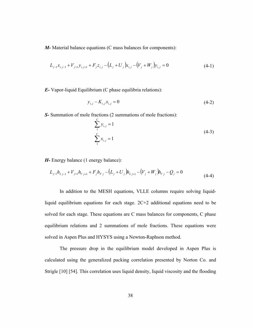
M- Material balance equations (C mass balances for components):

( ) ( ) 0,,,1,11,1 =+−+−++ ++−− jijjjijjjijjijjij yWVxULzFyVxL (4-1)

E- Vapor-liquid Equilibrium (C phase equilibria relations):

0,,, =− jijiji xKy (4-2)

S- Summation of mole fractions (2 summations of mole fractions):

1

1

1,

1,

=

=

∑

∑C

ji

C

ji

x

y (4-3)

H- Energy balance (1 energy balance):

( ) ( ) 011111 =−+−+−++ +++−− jjVjjjLjjjFjjVjjLj QhWVhULhFhVhL

(4-4)

In addition to the MESH equations, VLLE columns require solving liquid-

liquid equilibrium equations for each stage. 2C+2 additional equations need to be

solved for each stage. These equations are C mass balances for components, C phase

equilibrium relations and 2 summations of mole fractions. These equations were

solved in Aspen Plus and HYSYS using a Newton-Raphson method.

The pressure drop in the equilibrium model developed in Aspen Plus is

calculated using the generalized packing correlation presented by Norton Co. and

Strigle [10] [54]. This correlation uses liquid density, liquid viscosity and the flooding

39

parameter to obtain the pressure drop. For the liquid holdup calculation, the

equilibrium models developed in Aspen Plus used the Stichlmair correlation [53]. The

Stichlmair correlation requires the packing void fraction and surface area and three

Stichlmair correlation constants. These parameters were retrieved from vendor

information and Aspen Plus databases.

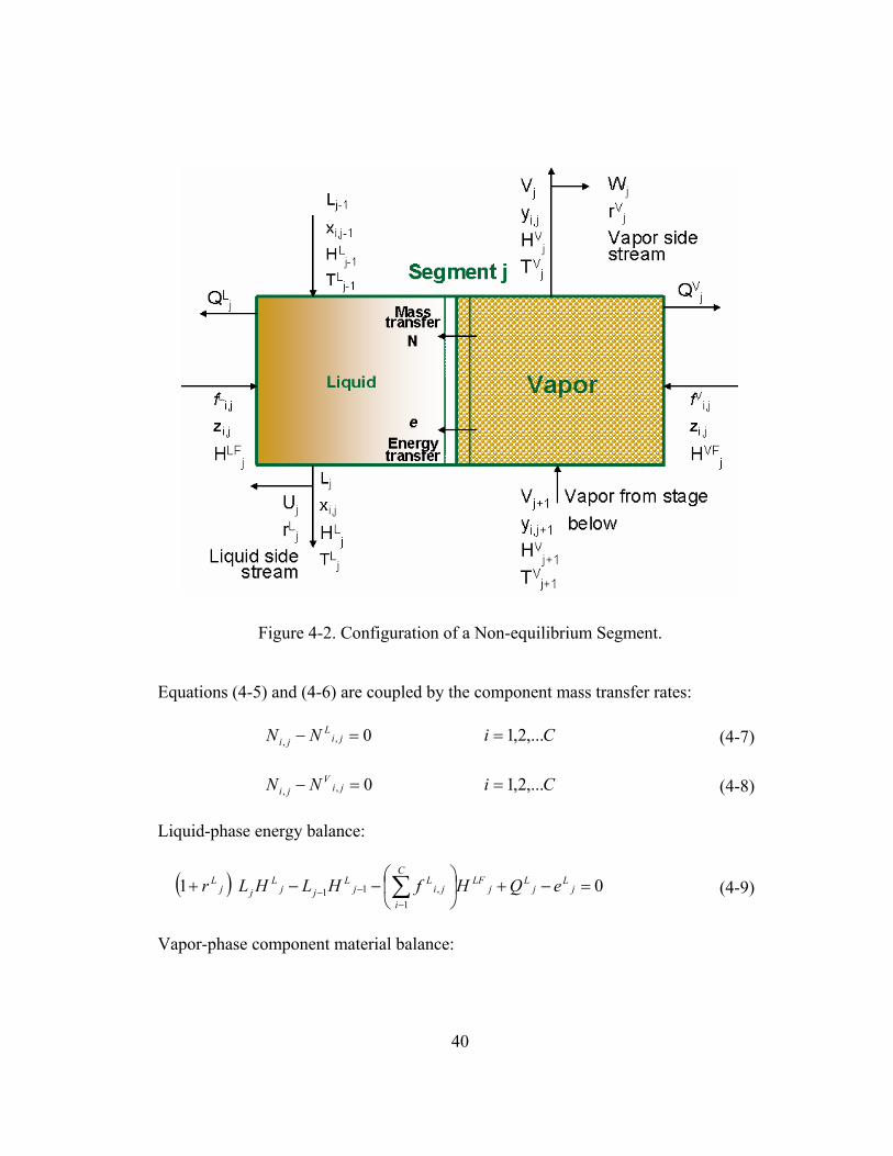
4.2.2 Non-equilibrium Approach

Entering segment j in Figure 4-2, are feed component i vapor and liquid flow

rates fij, liquid flow rate Lj-1, and vapor flow rate Vj+1. Leaving the segment, at

pressure Pj and temperature Tj, and enthalpy Hj are liquid and vapor flow rates Lj and

Vj. A fraction, rj, of these streams may be withdrawn in the side streams Uj and Wj.

Also leaving (+) or entering (-) the segment liquid and vapor phases are the heat

transfer rates Qj. Within the segment, mass transfer of components and heat transfer

occurs across the phase boundary at rates Ni,j and ej from the vapor phase to the liquid

phase (+) or vice versa (-). The super indices L and V represent the liquid and vapor

phase respectively. In the rate-based model, the mass and energy balances are

separated for each phase around a segment.

Liquid-phase component material balance:

( ) 01 ,,1,1, =−−−+ −− jiL

jiL

jijjijjL NfxLxLr Ci ,...2,1= (4-5)

Vapor-phase component material balance:

( ) 01 ,,1,1, =−−−+ ++ jiV

jiV

jijjijjV NfyVyVr Ci ,...2,1= (4-6)

40

Figure 4-2. Configuration of a Non-equilibrium Segment.

Equations (4-5) and (4-6) are coupled by the component mass transfer rates:

0,, =− jiL

ji NN Ci ,...2,1= (4-7)

0,, =− jiV

ji NN Ci ,...2,1= (4-8)

Liquid-phase energy balance:

( ) 011

,11 =−+⎟⎠

⎞⎜⎝

⎛−−+ ∑

−

−− jL

jL

jLF

C

iji

Lj

Ljj

Ljj

L eQHfHLHLr (4-9)

Vapor-phase component material balance:

41

( ) 011

,11 =−+⎟⎠

⎞⎜⎝

⎛−−+ ∑

−

++ jV

jV

jVF

C

iji

Vj

Vjj

Vjj

V eQHfHVHVr (4-10)

Where at the interface,

0=− jL

jV ee (4-11)

Summation of mole fractions, applied at the liquid-vapor interface:

1

1

1,

1,

=

=

∑

∑C

jiI

C

jiI

x

y (4-12)

Phase equilibrium for each component is assumed only at the liquid-vapor interface:

0,,, =− jiI

jiI

ji yxK (4-13)

In this work, two different steady state models were developed; one used the

equilibrium modeling approach and the other the non-equilibrium approach. The

purpose of these models was to provide an initial understanding of the process and to

evaluate the two different modeling methods when compared to the experimental

data. The steady state simulation was used as a starting point for the dynamic state

simulation.

Aspen-Plus was used to develop the steady state simulations because of the

thorough treatment of thermodynamic interactions and its status as a widely accepted

process simulator. Aspen-Plus provided a non-equilibrium solution while the

simulation developed in HYSYS was an equilibrium solution. HYSYS steady state

simulation was created as a first step for the development of the dynamic model. First

42

steady state equilibrium simulation in Aspen-Plus (Radfrac) was configured to match

results from the steady state simulation in HYSYS, which is also an equilibrium

model. This exercise helped to configure the two different simulators with the same

properties and parameters. Then rate-based simulation (Ratefrac) was performed in

Aspen-Plus, and the results compared with the equilibrium simulation.

4.2.3 First Distillation Region.

Eight different steady state points were studied in the first distillation region;

the raw data is presented in Table B-1. The system conditions were modified to

obtain different compositions at the top and bottom of the column. Table 4-2 presents

the controller set points used in the eight different steady state points studied.

Before the data collected from the process was used to validate the steady

state models it was first validated by calculating the process mass balance. The

difference in the material balance is due to the error in the composition measurement.

Table 4-2. Controller set points at first distillation region steady state values.

# Feed Flow Rate [lb/hr]

Distillate Flow Rate

[lb/hr]

Bottoms Flow Rate

[lb/hr]

Reflux Flow Rate

[lb/hr]

Reboiler Duty Rate

[kMBTU/hr]

Steam Flow Rate

[lb/hr]

Feed Temp

[F] 1 300 144.00 156.00 75 69.04 67 95 2 300 160.60 139.40 75 77.42 75 95 3 300 99.00 201.00 100 68.84 65 95 4 300 108.00 192.00 90 68.50 65 95 5 300 80.00 220.00 110 69.33 65 90 6 200 100.00 100.00 120 69.00 65 95 7 200 88.00 112.00 150 75.49 72 90 8 300 151.30 148.70 75 69.78 67 95

43

It was determined experimentally that the error in the composition

measurement was in the order of 1%. However, low (<2%) methanol and normal

pentane composition values increased the measurement error considerably. Since the

bottoms composition presented a trace of methanol, the composition data collected

from this stream was reconciled using the process material balance. The final

reconciled data is presented in Table 4-3.

Table 4-3. Reconciled Experimental Steady State Composition Data [w%]. First Distillation Region.

Feed Distillate Bottom #

MeOH C5 C6 MeOH C5 C6 MeOH C5 C6 1 4.06 49.34 46.60 6.74 93.08 0.18 1.58 8.97 89.45 2 3.96 51.52 44.52 6.85 92.96 0.19 0.63 3.78 95.58 3 3.27 43.65 53.09 8.92 90.83 0.25 0.48 20.41 79.11 4 3.67 44.15 52.18 8.66 91.29 0.06 0.86 17.63 81.50 5 2.95 41.77 55.29 8.75 90.92 0.33 0.84 23.89 75.27 6 3.28 51.10 45.62 4.34 95.26 0.40 2.22 6.93 90.85 7 3.02 48.06 48.92 6.33 93.64 0.03 0.43 12.24 87.33 8 4.06 52.11 43.83 5.99 93.84 0.17 2.10 9.64 88.26

4.2.3.1 Number of Stages/Segments Validation.

The number of stages in the equilibrium model was determined using the

HETP provided by the packing vendor and the total height of packing in the column.

Initially, the number of segments in the rate-based model was selected to match the

number of stages calculated for the equilibrium model. In order to validate the choice

of number of stages/segments, different simulations were performed adjusting the

number of equilibrium stages and segments in the models. The results presented in

Tables 4-4 and 4-5 correspond to the analysis of the steady state condition #2.

44

Table 4-4. Composition [weight %] results after variation in the number of equilibrium stages. First Distillation Region. Steady State Condition #2.

Product Component 13 Stages 26 Stages 52 Stages Experimental MeOH 7.40 7.397 7.397 6.85

C5 90.60 92.566 92.566 92.96 Distillate C6 2.01 0.037 0.037 0.19

MeOH 0.00 0.000 0.000 0.635 C5 6.50 4.232 4.232 3.782 Bottoms C6 93.50 95.768 95.768 95.583

Table 4-5. Composition [weight %] results after variation in the number of segments. First Distillation Region. Steady State Condition #2.

Product Component 13 Segments 26 Segments 52 Segments Experimental MeOH 8.244 8.250 8.250 6.85

C5 85.421 89.739 90.346 92.96 Distillate C6 6.335 2.011 1.404 0.19

MeOH 0.01 0.000 0.000 0.635 C5 20.23 16.241 15.681 3.782 Bottoms C6 79.77 83.759 84.319 95.583

The results indicated the selected number of equilibrium stages was correct,

since fewer stages gave lower agreement with the experimental data and more stages

did not improve the model performance compared with the experimental data.

Increasing the number of segments to 52 in the rate-based model did increase the

model performance when compared with the experimental data, matching the

predicted composition to that of the equilibrium model in five of the eight conditions

studied.

If the number of segments equals the number of stages the separation

predicted by the rate-based model is always going to be lower than the prediction

from the equilibrium model. This statement is explained by Peng [37], who described

a relationship between the equilibrium model and the non-equilibrium model. The

45

relationship established that when the number of segments in the rate-based model is

the same as the number of stages in the equilibrium model, the solution of both

models is identical if the interfacial area is infinitive. Since for a real packed column

the area in the rate-based model is finite, the separation predicted by the equilibrium

model is always going to be better than that predicted by the rate-based model when

the number of stages and segments is the same. Therefore the number of segments in

the rate-based model must be set to a higher value than the number of equilibrium

stages, otherwise the model under-predicts the separation.

4.2.3.2 Column Temperature Profile.

The following section includes the results obtained after analyzing the

temperature profiles in three different steady state conditions. Figure 4-3 indicates

that the equilibrium model gives a better approximation of the experimental data than

the non-equilibrium model. The similarities between the equilibrium model and the

experimental data suggest that the vapor pressure model was accurate and since the

vapor pressure model was the same for equilibrium and non-equilibrium models the

differences with the rate-based model may be associated with the mass and heat

transfer coefficient models which may not be accurate for this particular system.

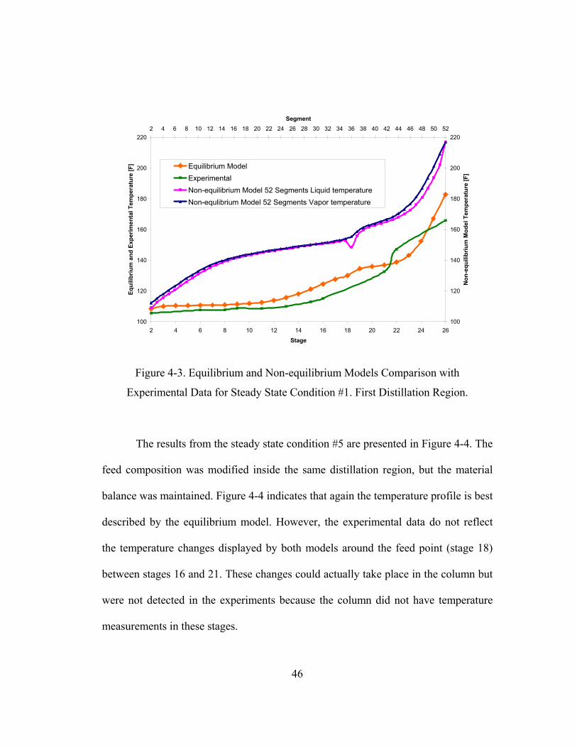
46

100

120

140

160

180

200

220

2 4 6 8 10 12 14 16 18 20 22 24 26

Stage

Equi

libriu

m a

nd E

xper

imen

tal T

empe

ratu

re [F

]

100

120

140

160

180

200

2202 4 6 8 10 12 14 16 18 20 22 24 26 28 30 32 34 36 38 40 42 44 46 48 50 52

Segment

Non

-equ

ilibr

ium

Mod

el T

empe

ratu

re [F

]

Equilibrium ModelExperimentalNon-equilibrium Model 52 Segments Liquid temperatureNon-equlibrium Model 52 Segments Vapor temperature

Figure 4-3. Equilibrium and Non-equilibrium Models Comparison with

Experimental Data for Steady State Condition #1. First Distillation Region.

The results from the steady state condition #5 are presented in Figure 4-4. The

feed composition was modified inside the same distillation region, but the material

balance was maintained. Figure 4-4 indicates that again the temperature profile is best

described by the equilibrium model. However, the experimental data do not reflect

the temperature changes displayed by both models around the feed point (stage 18)

between stages 16 and 21. These changes could actually take place in the column but

were not detected in the experiments because the column did not have temperature

measurements in these stages.

47

100

120

140

160

180

200

220

2 4 6 8 10 12 14 16 18 20 22 24 26

Stage

Equi

libriu

m a

nd E

xper

imen

tal T

empe

ratu

re [F

]

100

120

140

160

180

200

2202 4 6 8 10 12 14 16 18 20 22 24 26 28 30 32 34 36 38 40 42 44 46 48 50 52

Segment

Non

-equ

ilibr

ium

Mod

el T

empe

ratu

re [F

]




The equilibrium model and experimental data displayed a flat temperature

profile between stages 8 and 15, which was not exhibited by the non-equilibrium

model. Although the composition predicted by both models was roughly the same, the

temperature profile in this particular case was important because it indicated the

approximation to the azeotropic region. The results from the steady state condition #6

are presented in Figure 4-5.

48

100

120

140

160

180

200

220

2 4 6 8 10 12 14 16 18 20 22 24 26

Stage

Equi

libriu

m a

nd E

xper

imen

tal T

empe

ratu

re [F

]

100

120

140

160

180

200

2202 4 6 8 10 12 14 16 18 20 22 24 26 28 30 32 34 36 38 40 42 44 46 48 50 52

Segment

Non

-equ

ilibr

ium

Mod

el T

empe

ratu

re [F

]




The temperature profile given by the non-equilibrium model in Figure 4-5

again failed to indicate the constant temperature response starting in stage 6. In

contrast, the equilibrium model gave a very close temperature profile and, given that

the compositions predicted by both models were very similar, it was concluded that

the vapor pressure model used was accurate.

Since increasing the number of segments in the rate-based model improved in

the performance in the composition prediction for some of the steady state conditions

studied, the temperature profile was studied using different number of segments. The

results for condition #6 are presented in Figure 4-6.

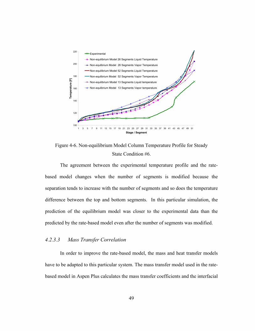
49

100

120

140

160

180

200

220

1 3 5 7 9 11 13 15 17 19 21 23 25 27 29 31 33 35 37 39 41 43 45 47 49 51

Stage / Segment

Tem

pera

ture

[F]

Experimental

Non-equilibrium Model 26 Segments Liquid Temperature

Non-equlibrium Model 26 Segments Vapor Temperature

Non-equilibrium Model 52 Segments Liquid Temperature

Non-equlibrium Model 52 Segments Vapor Temperature

Non-equilibrium Model 13 Segments Liquid temperature

Non-equlibrium Model 13 Segments Vapor temperature

Figure 4-6. Non-equilibrium Model Column Temperature Profile for Steady

State Condition #6.

The agreement between the experimental temperature profile and the rate-

based model changes when the number of segments is modified because the

separation tends to increase with the number of segments and so does the temperature

difference between the top and bottom segments. In this particular simulation, the

prediction of the equilibrium model was closer to the experimental data than the

predicted by the rate-based model even after the number of segments was modified.

4.2.3.3 Mass Transfer Correlation

In order to improve the rate-based model, the mass and heat transfer models

have to be adapted to this particular system. The mass transfer model used in the rate-

based model in Aspen Plus calculates the mass transfer coefficients and the interfacial

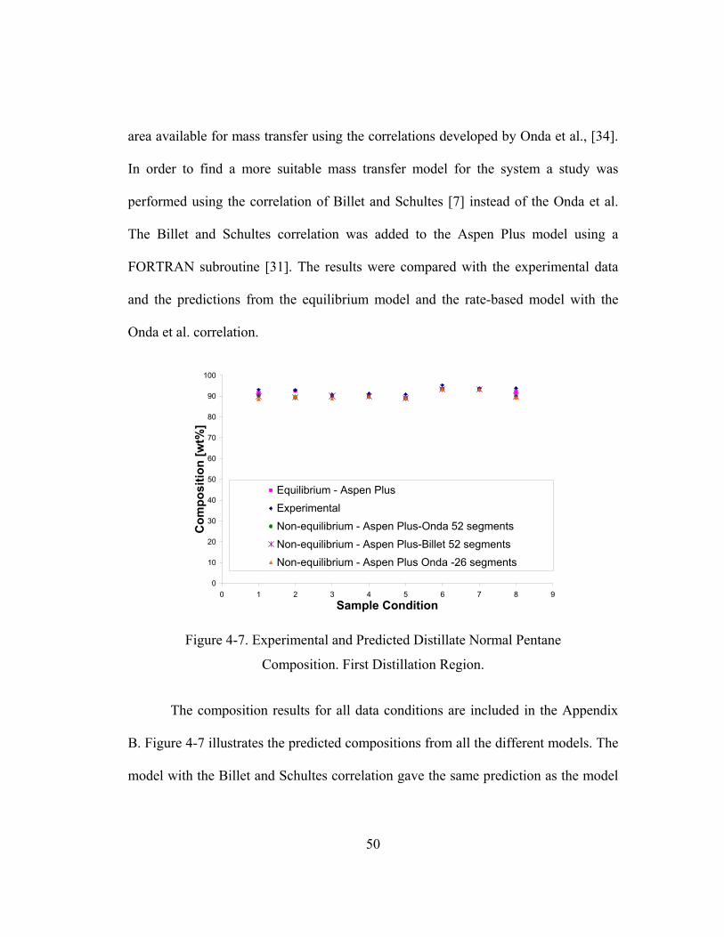
50

area available for mass transfer using the correlations developed by Onda et al., [34].

In order to find a more suitable mass transfer model for the system a study was

performed using the correlation of Billet and Schultes [7] instead of the Onda et al.

The Billet and Schultes correlation was added to the Aspen Plus model using a

FORTRAN subroutine [31]. The results were compared with the experimental data

and the predictions from the equilibrium model and the rate-based model with the

Onda et al. correlation.

0

10

20

30

40

50

60

70

80

90

100

0 1 2 3 4 5 6 7 8 9Sample Condition

Com

posi

tion

[wt%

]

Equilibrium - Aspen PlusExperimentalNon-equilibrium - Aspen Plus-Onda 52 segmentsNon-equilibrium - Aspen Plus-Billet 52 segmentsNon-equilibrium - Aspen Plus Onda -26 segments

Figure 4-7. Experimental and Predicted Distillate Normal Pentane

Composition. First Distillation Region.

The composition results for all data conditions are included in the Appendix

B. Figure 4-7 illustrates the predicted compositions from all the different models. The

model with the Billet and Schultes correlation gave the same prediction as the model

51

with the Onda et al. correlation for five of the eight conditions studied. For the other

three conditions the model with the Onda et al. correlation gave a closer agreement to

the experimental data.

4.2.3.4 Heat Transfer Correlation

The effect of the heat transfer correlation was studied by initially assuming the

temperatures of the liquid and vapor phases to be same and therefore eliminating the

interfacial heat transfer effect. Aspen Plus calculates the heat transfer coefficients for

the rate-based model, using the Chilton-Colburn analogy [21]. The analogy, described

in Equation (4-14), relates the mass transfer coefficients, avk , heat transfer

coefficients, tch , and Schmidt, Sc , and Prandtl, Pr, numbers.

( ) ( ) 32

32

Prmix

tcav Cp

hSck = ,

where mixCp = molar heat capacity [Joules/kg mole/K]

(4-14)

The non-equilibrium models were modified using a FORTRAN subroutine to

compare the model predictions with and without interfacial heat transfer. The

temperature profile predicted by the model with no interfacial heat transfer was the

same as the temperature of the liquid phase in the model with the interfacial heat

transfer calculations (Figure 4-8). However, there was a slight difference in the

composition prediction, after eliminating the heat transfer calculations in the interface

the rate-based models predicted a higher separation. The composition predictions

52

from all the models developed for the eight conditions studied in the first distillation

region are included in Appendix B. Figure 4-9 compares the normal pentane distillate

composition predictions from all the different models and the experimental data.

100

120

140

160

180

200

220

2 4 6 8 10 12 14 16 18 20 22 24 26

Stage

Tem

pera

ture

[F]

100

120

140

160

180

200

2202 4 6 8 10 12 14 16 18 20 22 24 26 28 30 32 34 36 38 40 42 44 46 48 50 52

Segment

Equilibrium Model

Experimental

Non-equilibrium Model 52 Segments Billet&Shultes Liquid temperature

Non-equilibrium Model 52 Segments - Onda et al. Liquid temperature

Non-equilibrium Model 52 Segments Billet&Shultes No Interfacial Heat

Non-equilibrium Model 52 Segments Onda et al. No Interfacial Heat

Figure 4-8. Column temperature profile for Steady State Condition #5.

The results indicated that the equilibrium models gave the best agreement

with the experimental data for the composition and temperature predictions. The rate-

based models gave good agreement with the experimental data and improved the

composition prediction as the number of segments was increased. However,

increasing the number of segments also moved the temperature profile away from the

experimental data. The predictions from the rate-based models were also improved

after the heat transfer in the interface was neglected. The rate-based model with the

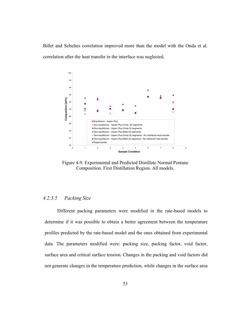
53

Billet and Schultes correlation improved more than the model with the Onda et al.

correlation after the heat transfer in the interface was neglected.

80

82

84

86

88

90

92

94

96

98

100

0 1 2 3 4 5 6 7 8 9

Sample Condition

Com

posi

tion

[wt%

]

Equilibrium - Aspen PlusNon-equilibrium - Aspen Plus Onda -26 segmentsNon-equilibrium - Aspen Plus-Onda 52 segmentsNon-equilibrium - Aspen Plus-Billet 52 segmentsNon-equilibrium - Aspen Plus-Onda 52 segments - No interfacial heat transferNon-equilibrium - Aspen Plus-Billet 52 segments - No intefacial heat transferExperimental

Figure 4-9. Experimental and Predicted Distillate Normal Pentane Composition. First Distillation Region. All models.

4.2.3.5 Packing Size

Different packing parameters were modified in the rate-based models to

determine if it was possible to obtain a better agreement between the temperature

profiles predicted by the rate-based model and the ones obtained from experimental

data. The parameters modified were: packing size, packing factor, void factor,

surface area and critical surface tension. Changes in the packing and void factors did

not generate changes in the temperature prediction, while changes in the surface area

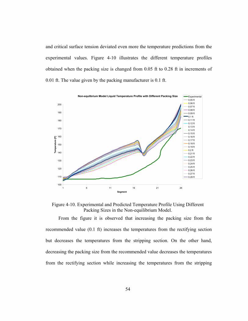
54

and critical surface tension deviated even more the temperature predictions from the

experimental values. Figure 4-10 illustrates the different temperature profiles

obtained when the packing size is changed from 0.05 ft to 0.28 ft in increments of

0.01 ft. The value given by the packing manufacturer is 0.1 ft.

Non-equlibrium Model Liquid Temperature Profile with Different Packing Size

100

110

120

130

140

150

160

170

180

190

200

1 6 11 16 21 26

Segment

Tem

pera

ture

[F]

Experimental0.05 ft0.06 ft0.07 ft0.08 ft0.09 ft0.1 ft0.11 ft0.12 ft0.13 ft0.14 ft0.15 ft0.16 ft0.17 ft0.18 ft0.19 ft0.2 ft0.21 ft0.22 ft0.23 ft0.24 ft0.25 ft0.26 ft0.27 ft0.28 ft

Figure 4-10. Experimental and Predicted Temperature Profile Using Different Packing Sizes in the Non-equilibrium Model.

From the figure it is observed that increasing the packing size from the

recommended value (0.1 ft) increases the temperatures from the rectifying section

but decreases the temperatures from the stripping section. On the other hand,

decreasing the packing size from the recommended value decreases the temperatures

from the rectifying section while increasing the temperatures from the stripping

55

section. It is concluded that modifying the packing size did not improve the rate-

based model temperature profile predictions.

4.2.4 Second Distillation Region

The composition data collected from the experiment presented less error that

the data collected from the first distillation region. This result was due to the fact than

there was a higher concentration of methanol in the sample.

Fourteen experimental steady state conditions were considered in the studied.

Table 4-6 summarized the operating conditions for each steady state condition.

Detailed results of the simulations from the second distillation region as well as the

detailed mass transfer models were presented by Mathijssen [31], with the

supervision of the author.

Table 4-6. Controller set points at second distillation region steady state values.

# Feed Flow

Rate [lb/hr]


[lb/hr]

Bottoms Flow Rate

[lb/hr]

Reflux Flow Rate

[lb/hr]

Reboiler Duty Rate

[kMBTU/hr]

Steam Flow Rate

[lb/hr]

Feed Temp

[F] 1 300 171 129 100 95 75 300 2 300 230 70 100 95 100 300 3 300 105 195 100 95 55 300 4 300 168 132 100 95 75 300 5 300 120 180 150 95 75 300 6 300 210 90 150 95 105 300 7 300 240 60 100 95 105 300 8 300 225 75 120 95 105 300 9 300 80 220 120 95 58 300 10 300 130 170 75 95 58 300 11 300 100 200 100 95 58 300 12 300 150 150 100 115 58 300 13 350 150 200 100 115 58 350 14 350 110 240 100 95 58 350

56

4.2.4.1 Mass Transfer Correlation

The predicted product compositions by the equilibrium and rate-based models

(using both Onda and Billet correlations) were close to the experimental data in all

the steady state conditions. All models predicted very similar compositions and the

data were consisted with the experimental data. Figure 4-11 and Table 4-7 present the

results comparison between the equilibrium and non-equilibrium models, and

experimental data for the steady state condition #1.

Table 4-7. Equilibrium and Non-equilibrium Models Comparison with Experimental

Data in Second Distillation Region. Steady State Condition #1.

DISTILLATE BOTTOM DISTILLATE BOTTOM

Experimental Equilibrium Comp Mass Frac (MeOH) 0.1162 0.7313 0.127 0.7078 Comp Mass Frac (n-C5) 0.8836 0.074 0.8729 0.0886 Comp Mass Frac (C6) 0.0002 0.1947 0.0001 0.2036

Non-Equilibrium (Billet and Schultes Correlation) Non-equilibrium (Onda Correlation)

Comp Mass Frac (MeOH) 0.1236 0.7073 0.1274 0.7073 Comp Mass Frac (n-C5) 0.8724 0.0893 0.8724 0.0894 Comp Mass Frac (C6) 0.0002 0.2034 0.0003 0.2033

Figure 4-11 indicates that the two non-equilibrium models as well as the

equilibrium model gave very similar temperature profiles. However, the equilibrium

model gave a closer agreement in the product composition.

Condition #2 was obtained by increasing the reboiler duty which sent the

methanol recovery to the top of the column. This was the condition that presented the

highest deviation between the models prediction and the experimental data. The

57

simulation results from this condition are presented in Table 4-8. It is observed that

again the non-equilibrium and the equilibrium models gave very similar results.

100

110

120

130

140

150

160

2 4 6 8 10 12 14 16 18 20 22 24 26

Stage

Tem

pera

ture

[F]

100

110

120

130

140

150

1602 4 6 8 10 12 14 16 18 20 22 24 26 28 30 32 34 36 38 40 42 44 46 48 50 52

Segment

Equilibrium Model

Experimental

Non-equilibrium model - Billet Correlation Liquidtemperature

Non-equilibrium model - Onda Correlation Liquidtemperature


Experimental Data. Second Distillation Region, Condition #1.

Table 4-8. Equilibrium and Non-equilibrium Models Comparison with Experimental

Data. Second Distillation Region, Condition #2.

DISTILLATE BOTTOM DISTILLATE BOTTOM

Experimental Equilibrium Comp Mass Frac (MeOH) 0.1505 0.9927 0.171 0.9627 Comp Mass Frac (n-C5) 0. 72059 0.0004 0.7162 0 Comp Mass Frac (C6) 0.129 0.0069 0.1128 0.0372

Non-Equilibrium (Billet and Schultes Correlation) Non-equilibrium (Onda Correlation)

Comp Mass Frac (MeOH) 0.1701 0.9657 0.1704 0.9647 Comp Mass Frac (n-C5) 0.7162 0.0000 0.7162 0.0001 Comp Mass Frac (C6) 0.1137 0.0343 0.1134 0.0352

A variation in the number of equilibrium stages in the equilibrium model and

the number of segments in the rated-base model gave the same results obtained in the

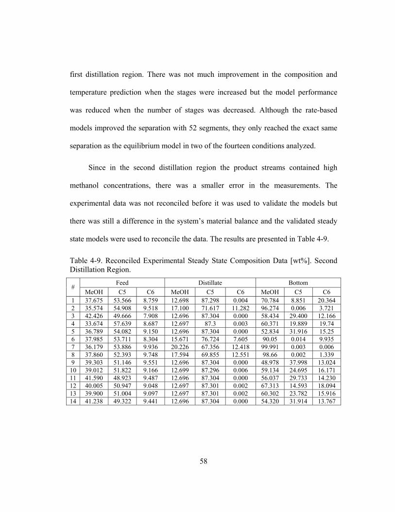
58

first distillation region. There was not much improvement in the composition and

temperature prediction when the stages were increased but the model performance

was reduced when the number of stages was decreased. Although the rate-based

models improved the separation with 52 segments, they only reached the exact same

separation as the equilibrium model in two of the fourteen conditions analyzed.

Since in the second distillation region the product streams contained high

methanol concentrations, there was a smaller error in the measurements. The

experimental data was not reconciled before it was used to validate the models but

there was still a difference in the system’s material balance and the validated steady

state models were used to reconcile the data. The results are presented in Table 4-9.

Table 4-9. Reconciled Experimental Steady State Composition Data [wt%]. Second Distillation Region.

Feed Distillate Bottom #

MeOH C5 C6 MeOH C5 C6 MeOH C5 C6 1 37.675 53.566 8.759 12.698 87.298 0.004 70.784 8.851 20.364 2 35.574 54.908 9.518 17.100 71.617 11.282 96.274 0.006 3.721 3 42.426 49.666 7.908 12.696 87.304 0.000 58.434 29.400 12.166 4 33.674 57.639 8.687 12.697 87.3 0.003 60.371 19.889 19.74 5 36.789 54.082 9.150 12.696 87.304 0.000 52.834 31.916 15.25 6 37.985 53.711 8.304 15.671 76.724 7.605 90.05 0.014 9.935 7 36.179 53.886 9.936 20.226 67.356 12.418 99.991 0.003 0.006 8 37.860 52.393 9.748 17.594 69.855 12.551 98.66 0.002 1.339 9 39.303 51.146 9.551 12.696 87.304 0.000 48.978 37.998 13.024

10 39.012 51.822 9.166 12.699 87.296 0.006 59.134 24.695 16.171 11 41.590 48.923 9.487 12.696 87.304 0.000 56.037 29.733 14.230 12 40.005 50.947 9.048 12.697 87.301 0.002 67.313 14.593 18.094 13 39.900 51.004 9.097 12.697 87.301 0.002 60.302 23.782 15.916 14 41.238 49.322 9.441 12.696 87.304 0.000 54.320 31.914 13.767

59

4.3 Model Responses Discussion and Comparison with

Experimental Data.

Although the equilibrium and non-equilibrium models gave different

temperature profiles in the first distillation region, the compositions predicted were

very similar. In the last set of conditions studied, the compositions were the same and,

in the first set of conditions, the difference was less than 0.1%. For this particular

region the non-equilibrium model failed to report the trace of cyclohexane present in

the distillate stream. The most important difference between the two models was

perhaps the temperature response for the stages with azeotropic conditions. Although

the rate-based model predicted the azeotropic composition in the distillate stream, the

temperature profile did not indicate azeotropic behavior.

The temperature profiles given by the non-equilibrium models and the

equilibrium model in the second distillation region were very similar. The models

also gave very similar compositions. There was not a visible difference between the

non-equilibrium models using the two different correlations for the mass transfer

coefficients. An experimental study for the particular packing used in the column is

needed to develop good correlations that could improve the non-equilibrium models.

However, there is very little room for improvement since for this particular system

the equilibrium models gave very good performance.

60

There are two important remarks related to the temperature response given by

the equilibrium and non-equilibrium models. First, the temperature difference

between the experimental data and the equilibrium model changed between

distillation regions but remained roughly constant to the predictions of the non-

equilibrium model. Second, the slope of the temperature profile obtained from the

experiments outside the azeotropic condition was closer to the slope in the profile

predicted by the non-equilibrium model than the one predicted by the equilibrium

model. The fact that the temperature profile from the equilibrium model in the

azeotropic region gave a better agreement with experimental data than with the non-

equilibrium model may suggest that more segments need to be added to the rectifying

section of the column in the non-equilibrium model. This is also concluded based on

the composition prediction in the first distillation region, where the non-equilibrium

model did not always predicted the separation obtained in the experiments.

The equilibrium approach was selected to study the system behavior and to

develop further work on online modeling reconciliation since it showed good

agreement with the experimental data, and less CPU resources were needed to

implement this simulation.

61

Chapter 5. Dynamic State Model for Azeotropic Distillation

The purpose of this part of the research was to develop a high fidelity dynamic

model for azeotropic distillation that could be maintained using online reconciliation

with process data and could be used to test control strategies before their

implementation in a real plant. In order to select the most suitable simulator to

develop the simulation, several process simulators capabilities were considered. The

most important considerations were strong model libraries, possible interface with the

experimental plant control software and dynamic capabilities.

5.1 Model description

The dynamic model configuration was the same as the steady state model

configuration described in the previous section in Table 4-1. The equilibrium steady

state model developed in HYSYS was used as a basis for the dynamic model. Besides

its dynamic capabilities and strong thermodynamic libraries, HYSYS was selected as

a dynamic simulation package because of its interface connection to DeltaV, the

control system used in the experimental plant, which facilitated the connection

between the model and the controller in the plant control system.

As concluded in the previous section, the steady state simulation indicated that

the equilibrium model provided close agreement between the predicted process

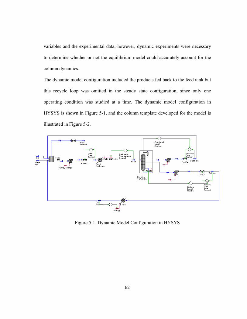
62

variables and the experimental data; however, dynamic experiments were necessary

to determine whether or not the equilibrium model could accurately account for the

column dynamics.

The dynamic model configuration included the products fed back to the feed tank but

this recycle loop was omitted in the steady state configuration, since only one

operating condition was studied at a time. The dynamic model configuration in

HYSYS is shown in Figure 5-1, and the column template developed for the model is

illustrated in Figure 5-2.

Figure 5-1. Dynamic Model Configuration in HYSYS

63

Figure 5-2. Column Template used in Dynamic Model.

The dynamic model included the product recycle loop because the feed

composition changed from the moment the step change was performed. After the data

from the experiments were collected, the operating conditions were recreated in the

simulation environment and the results compared with the experimental data. If the

feed composition between the simulation and the experiments was more than 5% off,

the same experimental conditions were used again to check repeatability. This

situation usually occurred when two step changes were performed in reduced

amounts of time and, as a consequence, the system was not in steady state when the

second change was performed.

64

5.1.1 HYSYS Pressure and Liquid Hold-up Model The column vapor pressure drop and liquid hold-up in the dynamic

equilibrium model developed in HYSYS are calculated using the Robbins correlation

[42] presented in Equation (5-1).

[ ]

54

83

1.05.05.0

5.05.0

423

1.02

3

107.2

104.7

204.62

20075.0

10000,20

4.010 44

−

−

×=

×=

⎥⎦

⎤⎢⎣

⎡⎥⎦

⎤⎢⎣

⎡=

⎥⎦

⎤⎢⎣

⎡

⎥⎥⎦

⎤

⎢⎢⎣

⎡=

⎥⎦

⎤⎢⎣

⎡+=Δ

C

C

FLL

FGG

GCL

GCP

pd

Lf

pd

gf

LCf

fLCf

ff

μρ

ρ

(5-1)

In Equation (5-1), G represents the gas loading and fG the gas loading factor.

L represents the liquid loading and fL the liquid loading factor. PΔ is the specific

pressure drop. The dry-bed packing factor, pdF , is directly related to the specific

pressure drop through dry bed, pbPΔ . The correlation is described by Equation (5-2).

228 278

075.0107.2

s

dbdbgpd F

PGPF Δ

=⎥⎦⎤

⎢⎣⎡Δ

⎥⎦

⎤⎢⎣

⎡×=

ρ

(5-2)

5.1.2 HYSYS Heat Transfer Coefficient

The column’s external surface heat transfer coefficient directly influences the

heat loss experienced by the column. HYSYS allows the user to specify a simple or a

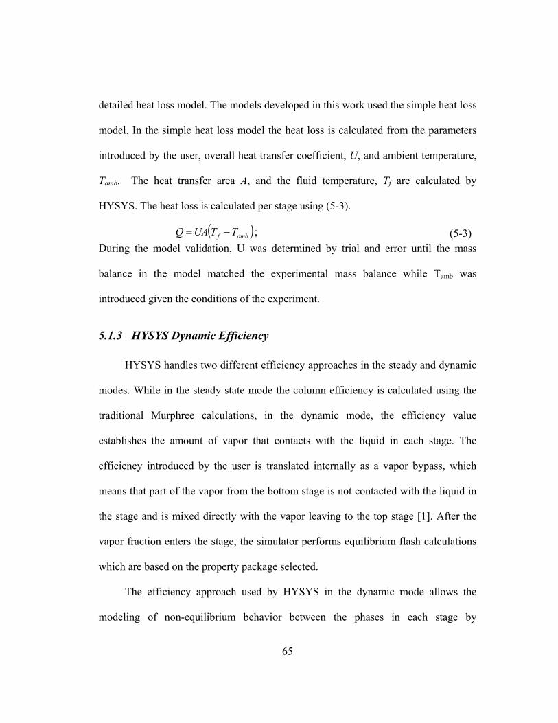
65

detailed heat loss model. The models developed in this work used the simple heat loss

model. In the simple heat loss model the heat loss is calculated from the parameters

introduced by the user, overall heat transfer coefficient, U, and ambient temperature,

Tamb. The heat transfer area A, and the fluid temperature, Tf are calculated by

HYSYS. The heat loss is calculated per stage using (5-3).

( )ambf TTUAQ −= ; (5-3)During the model validation, U was determined by trial and error until the mass

balance in the model matched the experimental mass balance while Tamb was

introduced given the conditions of the experiment.

5.1.3 HYSYS Dynamic Efficiency

HYSYS handles two different efficiency approaches in the steady and dynamic

modes. While in the steady state mode the column efficiency is calculated using the

traditional Murphree calculations, in the dynamic mode, the efficiency value

establishes the amount of vapor that contacts with the liquid in each stage. The

efficiency introduced by the user is translated internally as a vapor bypass, which

means that part of the vapor from the bottom stage is not contacted with the liquid in

the stage and is mixed directly with the vapor leaving to the top stage [1]. After the

vapor fraction enters the stage, the simulator performs equilibrium flash calculations

which are based on the property package selected.

The efficiency approach used by HYSYS in the dynamic mode allows the

modeling of non-equilibrium behavior between the phases in each stage by

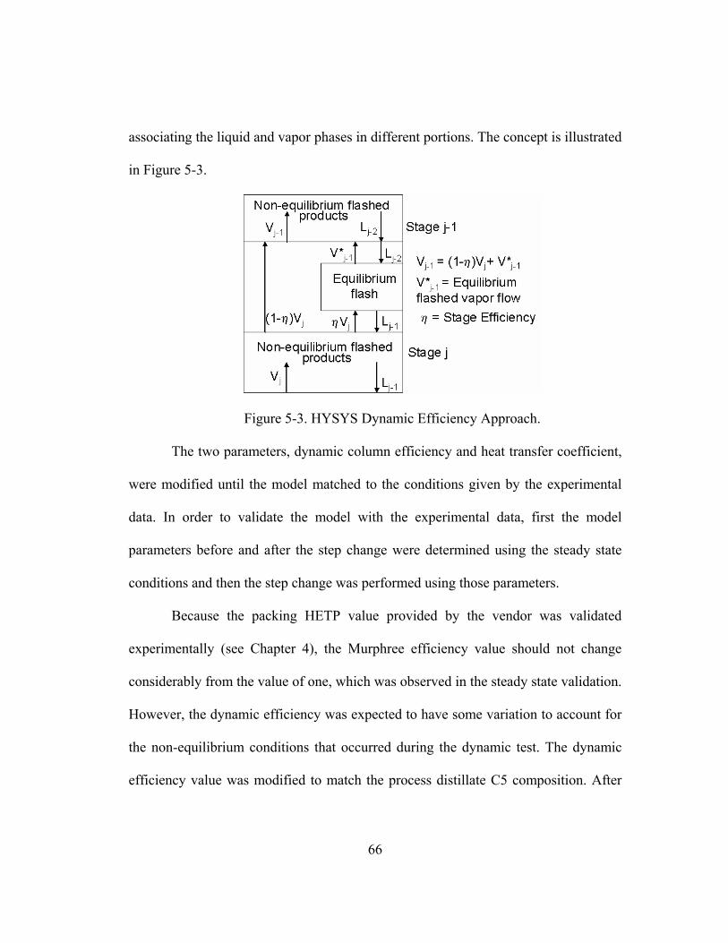
66

associating the liquid and vapor phases in different portions. The concept is illustrated

in Figure 5-3.

Figure 5-3. HYSYS Dynamic Efficiency Approach.

The two parameters, dynamic column efficiency and heat transfer coefficient,

were modified until the model matched to the conditions given by the experimental

data. In order to validate the model with the experimental data, first the model

parameters before and after the step change were determined using the steady state

conditions and then the step change was performed using those parameters.

Because the packing HETP value provided by the vendor was validated

experimentally (see Chapter 4), the Murphree efficiency value should not change

considerably from the value of one, which was observed in the steady state validation.

However, the dynamic efficiency was expected to have some variation to account for

the non-equilibrium conditions that occurred during the dynamic test. The dynamic

efficiency value was modified to match the process distillate C5 composition. After

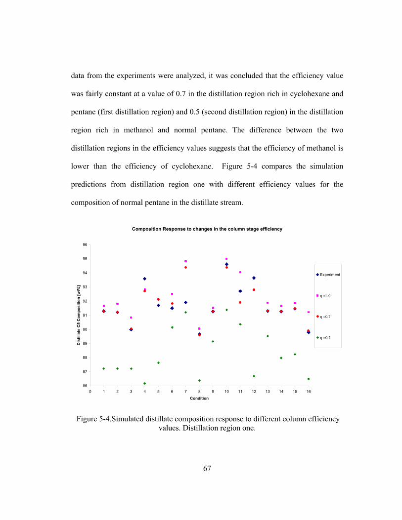
67

data from the experiments were analyzed, it was concluded that the efficiency value

was fairly constant at a value of 0.7 in the distillation region rich in cyclohexane and

pentane (first distillation region) and 0.5 (second distillation region) in the distillation

region rich in methanol and normal pentane. The difference between the two

distillation regions in the efficiency values suggests that the efficiency of methanol is

lower than the efficiency of cyclohexane. Figure 5-4 compares the simulation

predictions from distillation region one with different efficiency values for the

composition of normal pentane in the distillate stream.

Composition Response to changes in the column stage efficiency

86

87

88

89

90

91

92

93

94

95

96

0 1 2 3 4 5 6 7 8 9 10 11 12 13 14 15 16

Condition

Dis

tilla

te C

5 C

ompo

sitio

n [w

t%]

Experiment

η =1.0

η =0.7

η =0.2

Figure 5-4.Simulated distillate composition response to different column efficiency values. Distillation region one.

68

Figure 5-4 indicated two conditions (4 and 12) where the simulation did not

reach the experimental value, even with an efficiency of one. These conditions were

characterized by higher reboiler duties and therefore higher distillate flow rates than

the other conditions. The difference between the simulated composition at 0.7 column

efficiency and the composition obtained from the experiment is still lower than 3%.

The difference between predicted and experimental data is also due to the

error presented in the experimental data which is observed by the difference in the

material balance (see Table 5-1).

Table 5-1. Experimental data material balance error. First distillation region.

Condition #

Feed w%

MeOH

Feed w% C5

Feed w% C6

Distillate w%

MeOH

Distillate w% C5

Distillate w% C6

1 3.67 44.15 52.18 8.65 91.29 0.06 2 3.49 43.12 53.39 8.73 91.21 0.06 3 2.98 40.59 56.43 9.98 89.99 0.03 4 3.94 51.86 44.20 6.33 93.59 0.08 5 4.00 51.50 44.50 8.10 91.70 0.20 6 3.90 51.00 45.10 8.30 91.50 0.20 7 4.47 41.00 54.53 8.09 91.91 0.00 8 2.77 40.58 56.66 10.16 89.65 0.18 9 3.13 42.56 54.30 8.46 91.26 0.28

10 3.11 48.26 48.64 5.20 94.61 0.19 11 3.05 45.46 51.49 7.15 92.71 0.14 12 3.02 48.06 48.92 6.33 93.64 0.03 13 3.23 44.90 51.87 8.62 91.30 0.08 14 3.14 42.56 54.30 8.46 91.26 0.28 15 3.75 43.82 52.43 8.49 91.46 0.05 16 5.41 48.29 46.30 10.17 89.79 0.04

69

Mass Balance Difference MeOH C5 C6

Condition #

Bottom w%

MeOH

Bottom w% C5

Bottom w% C6 (PPH) (PPH) (PPH)

1 0.87 17.63 81.50 0.74 6.99 -7.73 2 0.02 22.69 77.29 2.76 1.12 -3.89 3 0.00 24.15 75.85 1.31 -1.01 -0.30 4 0.00 11.80 88.20 2.29 -2.92 0.62 5 0.00 12.70 87.30 0.05 -0.11 0.06 6 0.00 14.10 85.90 -0.18 -0.10 0.29 7 3.19 23.05 73.76 -0.26 -3.72 3.98 8 0.04 23.72 76.25 -0.61 -5.84 6.46 9 0.16 23.06 76.79 1.72 -0.67 -1.05

10 0.04 16.74 83.22 1.90 -0.82 -1.08 11 0.06 18.28 81.66 0.96 1.62 -2.57 12 0.00 15.06 84.94 1.05 -0.41 -0.64 13 0.15 19.87 79.98 1.08 6.27 -7.35 14 0.15 23.06 76.79 1.93 0.70 -2.62 15 0.00 22.28 77.72 3.71 3.20 -6.92 16 0.00 24.07 75.93 5.02 0.20 -5.22

The mass balance difference in Table 5-1 is calculated by subtracting from the

amount of each component in the feed the amounts of each component in the distillate

and bottom streams. The mass balance difference is explained by the error introduced

in the compositions analysis which was estimated to be ±3%. The error introduced by

the flow measurement was negligible.

During the model validation analysis it was determine that the different

combinations of heat transfer coefficient and efficiency values gave the same

composition outputs. For this reason the efficiency value was held constant at a value

of 0.7 in the first region and 0.5 in the second region, while the heat transfer

coefficient was modified to match the mass balance of the model with the process.

70

After heat transfer coefficient was modified it was held constant while the efficiency

value was modified to achieve the desire composition.

5.2 Control configuration.

The process was operated initially using a traditional control configuration

without advanced control implementation. Table 5-2 describes the pairing of

manipulated and control variables. This configuration was selected based on previous

experimentation [44].

Table 5-2. Pairing of Manipulated Variables with Controlled Variables.

Manipulated Variables Controlled Variables Control Strategy

Feed flow valve position Feed Flow PID

Reflux flow valve position Reflux Flow PID

Reboiler steam flow valve position Steam Flow PID

Preheater steam flow valve position Feed Temperature PID

Nitrogen flow valve position Pressure PID

Distillate flow Accumulator Level PID - Cascade

Bottom flow Bottom Level PID – Cascade

71

5.3 Step change responses.

Binary distillation of cyclohexane and normal heptane [44] was performed

previously to test the equipment. The results of this study indicated that temperature

measurements from stages 9 and 16 were the best fit for inferential control of

composition. However, after the first series of step changes were performed in the

azeotropic system, comparisons between experimental and simulated temperatures in

the column indicated that the temperature measurements from the overhead and stage

16 gave the best match with the simulation results for the temperature in the

rectifying section. The overhead temperature was the fastest temperature to arrive at

steady state. Likewise, the temperature measurement from stage 22 provided the best

match of the bottom temperatures.

Using the control configuration described in the previous section, a series of

closed loop step changes were performed in the system to validate the dynamic

model. The variables manipulated during the test were: feed flow rate, feed

temperature, reflux flow rate, and reboiler duty. Each variable was changed while all

the other variables in the system were held constant by their controllers. The hold-ups

in the bottom of the column and reflux drum as well as the pressure in the column

were maintained at a constant set-point by their individual control loops. The

manipulated variables set points for each condition in the test are listed in Table 5-3

for the first and Table 5-4 for the second distillation region. The data collected from

the experiments are included in the Appendix as well as the simulated data.

72

Table 5-3. Dynamic test process variables set points. First Distillation Region

Condition #

Feed Flow Rate

[lb/hr]

Bottom Flow Rate

[lb/hr]

Distillate flow Rate

[lb/hr]

Reflux Flow Rate

[lb/hr]

Feed Temp [F]

Steam Flow Rate

[lb/hr]

Reboiler Duty

[MMBTU/hr] 1 300 201.48 98.52 90 95 65 68.35 2 300 212.19 87.81 110 95 65 69.10 3 300 223.55 76.45 150 95 72 76.43 4 300 149.50 150.50 75 95 72 75.21 5 300 152.52 147.48 75 95 72 75.44 6 300 156.84 143.16 75 95 65 68.11 7 200 142.46 57.54 150 90 65 69.30 8 200 140.00 60.00 150 90 72 75.81 9 300 213.22 86.78 110 90 65 69.22

10 200 118.10 81.90 110 90 65 68.69 11 200 129.14 70.86 150 90 72 75.50 12 300 173.49 126.51 150 95 72 76.61 13 300 203.65 96.35 110 110 65 68.70 14 300 215.24 84.76 110 90 65 69.11 15 300 211.22 88.78 110 95 65 69.05 16 300 189.75 110.25 110 110 65 68.98

Table 5-4. Dynamic test process variables set points. Second Distillation Region

Condition #

Feed Flow Rate

[lb/hr]

Bottom Flow Rate

[lb/hr]


[lb/hr]

Reflux Flow Rate

[lb/hr]

Feed Temp [F]

Steam Flow Rate

[lb/hr]

Reboiler Duty

[MMBTU/hr]

1 300.00 89.55 210.45 150.00 95.00 105.00 111.56 2 300.00 62.56 237.44 100.00 95.00 105.00 111.64 3 300.00 169.27 130.73 75.00 95.00 58.00 62.51 4 300.00 200.09 99.91 100.00 95.00 58.00 62.80 5 300.00 71.47 228.53 100.00 95.00 100.00 105.88 6 300.00 199.88 100.12 100.00 95.00 55.00 60.98 7 300.00 199.88 100.12 100.00 95.00 55.00 60.98 8 300.00 127.20 172.80 100.00 95.00 75.00 80.09 9 300.00 184.59 115.41 100.00 95.00 58.00 62.76

10 200.00 90.41 109.59 100.00 95.00 58.00 61.99 11 200.00 90.15 109.85 100.00 95.00 58.00 62.04 12 200.00 136.97 63.03 100.00 95.00 58.00 62.06 13 350.00 199.92 150.08 100.00 110.00 58.00 62.89 14 350.00 239.95 110.05 100.00 95.00 58.00 62.38 15 300.00 188.46 111.54 100.00 95.00 58.00 62.88 16 300.00 149.97 150.03 100.00 115.00 58.00 62.31

Each condition in Tables 5-3 and 5-4 represents the steady state values from before

and after a step change was performed.

73

The following sections contain the most relevant experimental and simulated

data from the series of step changes performed on the system, other data are provided

in the Appendix. First, the experimental results for the temperature responses in the

column are presented. These results are divided into two plots, one with temperatures

from the rectifying section (overhead and stages 6, 8, 9 11, 13, 15 and 16) and the

other with the temperatures from the stripping section (stages 21 and 22 and column

bottoms and boilup stream). After presenting the experimental data, a temperature

measurement from the rectifying section and a temperature measurement from the

stripping section (temperatures from stages 16 and 22) are plotted separately with

their respective simulated value. Following the model validation a figure with the

simulated compositions is presented. A table with a summary of the experimental and

simulated conditions before and after the step change is included.

5.3.1 Changes in reflux flow rate:

5.3.1.1 First Distillation Region

Reflux flow changes were performed, seeking to move the operating point in

and out of the azeotropic region. The series of step changes in the reflux flow rate

started at low flow rates (75 lb/hr) and ended at high flow rates (150 lb/hr), where the

normal-pentane / methanol azeotrope was recovered in the distillate product. The

results from a positive step change in the reflux flow rate from 90 to 110 lb/hr are

presented below. Figure 5-5 illustrates the temperatures responses from the rectifying

74

section and Figure 5-6 illustrates the responses from the stripping section. Figure 5-7

presents a comparison between the predicted and experimental temperatures and

Figure 5-8 shows the predicted composition profile. Table 5-5 includes a summary of

the conditions before and after the test was performed.

Table 5-5. Step change in Reflux Flow Rate 90 to 110 lb/hr. Simulation and Process Results. First Distillation Region.

Before (90 lb/hr) After (110 lb/hr) FEED DISTILLATE BOTTOM FEED DISTILLATE BOTTOM

Mass Flow [lb/hr] 300.00 98.52 201.48 300.00 87.81 212.19

Experimental Mass Fraction Composition FEED DISTILLATE BOTTOM FEED DISTILLATE BOTTOM

Methanol 0.0367 0.0865 0.0087 0.0349 0.0873 0.0002 n-Pentane 0.4415 0.9129 0.1763 0.4312 0.9121 0.2269

Cyclohexane 0.5218 0.0006 0.8150 0.5339 0.0006 0.7729

Simulated Mass Fraction Composition FEED DISTILLATE BOTTOM FEED DISTILLATE BOTTOM


Cyclohexane 0.5218 0.0008 0.7776 0.5339 0.0009 0.7545

75

Figure 5-5. Rectifying Zone Temperature Response to a Positive Step Change (90 to 110 lb/hr) in the Reflux Flow Rate. First Distillation Region.

Rec

tifyi

ng Z

one

Tem

pera

ture

Res

pons

e to

Pos

itive

Ste

p C

hang

e in

Ref

lux

Flow

Rat

e

102

103

104

105

106

107

108

109

110

111

112

020

4060

8010

0

Tim

e [m

in]

Temperature [F]

708090100

110

120

130

140

150

160

Reflux Flow Rate [lb/hr]

Tem

pera

ture

Ove

rhea

d va

pTe

mpe

ratu

re T

op S

tage

6Te

mpe

ratu

re S

tage

8Te

mpe

ratu

re S

tage

9Te

mpe

ratu

re S

tage

11

Tem

pera

ture

Sta

ge 1

3Te

mpe

ratu

re S

tage

15

Tem

pera

ture

Sta

ge 1

6R

eflu

x Fl

ow R

ate

Feed

Flo

w =

300

lb/h

rR

eflu

x Fl

ow =

90-

110

lb/h

rS

team

Flo

w =

65

lb/h

rD

uty

= 69

KB

TU/h

r

76

Figure 5-6. Stripping Zone Temperature Response to a Positive Step Change (90 to 110 lb/hr) in the Reflux Flow Rate. First Distillation Region.

Strip

ping

Zon

e Te

mpe

ratu

re R

espo

nse

to P

ositi

ve S

tep

Cha

nge

in R

eflu

x Fl

ow R

ate

120

125

130

135

140

145

150

155

160

165

170

020

4060

8010

0

Tim

e [m

in]

Temperature [F]

708090100

110

120

130

140

150

160


Tem

pera

ture

Sta

ge 2

1Te

mpe

ratu

re S

tage

22

Tem

pera

ture

boi

l up

Tem

pera

ture

Bot

t col

Ref

lux

Flow

Rat

e

Feed

Flo

w =

300

lb/h

rR

eflu

x Fl

ow =

90-

110

lb/h

rS

team

Flo

w =

65

lb/h

rD

uty

= 69

KB

TU/h

r

77

Figure 5-7. Simulated and Experimental Temperature Responses to a Positive Step Change (90 to 110 lb/hr) in the Reflux Flow Rate. First Distillation Region.

Mod

el T

empe

ratu

re R

espo

nse

Valid

atio

n

020406080100

120

010

2030

4050

6070

8090

100

Tim

e (m

in)

Reflux Flow Rate (lb/hr)

100

110

120

130

140

150

160

170

180

190

200

Temperature (F)

Ref

lux

Flow

Rat

eSi

mul

ated

Ref

lux

Flow

Rat

e

Tem

pera

ture

Sta

ge 1

6Si

mul

atio

n Te

mpe

ratu

re S

tage

16

Tem

pera

ture

Sta

ge 2

2S

imul

atio

n Te

mpe

ratu

re S

tage

22

Col

umn

Effic

ienc

y =

0.7

Col

umn

Hea

t Tra

nsfe

r Coe

ffici

ent =

5.78

- 5.

48 B

TU/h

r*ft2

*FFe

ed F

low

Rat

e=30

0 lb

/hr

Ref

lux

Flow

Rat

e= 9

0-11

0 lb

/hr

Ste

am F

low

Rat

e =

65 lb

/hr

Dis

tilla

te F

low

Rat

e=98

.52

- 87.

81 lb

/hr

78

Figure 5-8. Composition Response to a Positive Step Change (90 to 110 lb/hr) in the Reflux Flow Rate. First Distillation Region.

Com

posi

tion

Res

pons

e to

a P

ositi

ve S

tep

Cha

nge

in th

e R

eflu

x Fl

ow R

ate

020406080100

120

010

2030

4050

6070

8090

100

Tim

e (m

in)


707580859095100

Composition (Weight % )

Sim

ulat

ed R

eflu

x Fl

ow R

ate

Dis

tilla

te C

5 C

ompo

sitio

nBo

ttom

C6

Com

posi

tion

Dis

tilla

te C

5 co

mpo

sitio

nE

xper

imen

tal

= 91

.29

- 91.

21 w

t%S

imul

ated

= 9

1.29

- 91

.20

wt%

Bot

tom

C6

Com

posi

tion

Exp

erim

enta

l = 8

1.50

- 77

.29

wt%

Sim

ulat

ed =

77.

77 -

75.5

wt%

Feed

Com

posi

tion

Bef

ore

Ste

p Te

stM

etha

nol =

3.6

7 w

t%N

orm

al p

enta

ne =

52.

18 w

t%C

yclo

hexa

ne =

44.

15 w

t%

Feed

Com

posi

tion

Afte

r Ste

p Te

stM

etha

nol =

3.4

9 w

t%N

orm

al p

enta

ne =

53.

39 w

t%C

yclo

hexa

ne =

43.

12 w

t%

Col

umn

Effic

ienc

y =

0.7

Col

umn

Hea

t Tra

nsfe

r Coe

ffici

ent =

5.78

- 5.

48 B

TU/h

r*ft2

*F

79

Temperatures from the rectifying section increased with the reflux flow rate.

This is not a typical response; in ordinary distillation, temperatures are expected to

decrease as the reflux flow rate is increased. The simulation was repeated without the

feed composition disturbance and it was determined that the increase in the

temperature response was introduced by the disturbance. Figure 5-9 illustrates the

simulation results after the step change was performed without introducing the feed

concentration disturbances.

The distillate compositions predicted by the model gave very close agreement

with the distillate compositions measured in the experiment. There is a 4% error in

the initial condition measured compositions in the bottom stream, which is reflected

in the experiments difference in the material balance. This was the largest difference

presented between the predicted simulation and the experimental data in the model

validation. The heat transfer coefficient was maintained fairly constant during the

experiment, it changed from 5.78 to 5.48 BTU/hr*ft2*F after the step change was

performed. The efficiency value was set at 0.7.

80

Figure 5-9. Simulation Temperature Response to a Positive Step Change (90 to 110 lb/hr) in the Reflux Flow Rate without feed composition disturbance. First Distillation

Region.

708090100

110

120

130

140

150 80

081

082

083

084

085

086

087

088

089

090

0

Tim

e [m

in]

Flow Rate [lb/hr]

9499104

109

114

119

Temperature [F]

Ref

lux

Flow

Sim

ulat

ion

Ove

rhea

d

Sim

ulat

ion

Stag

e 3

Sim

ulat

ion

Stag

e 4

Feed

Flo

w =

300

lb/h

rR

eflu

x Fl

ow =

90-

110

lb/h

rS

team

Flo

w =

65

lb/h

rD

uty

= 69

- 69

KB

TU/h

rFe

ed C

ompo

sitio

nM

etha

nol 2

.99%

n-P

enta

ne 4

0.59

%C

yclo

hexa

ne 5

6.43

%

81

5.3.1.2 Second Distillation Region

The experimental results for temperature responses in the column’s rectifying

and stripping sections to a negative step change in the reflux flow rate are presented

in Figure 5-10 and Figure 5-11 respectively. Figure 5-12 illustrates a comparison

between the predicted and the experimental responses and Figure 5-13 presents the

predicted composition profile. Table 5-6 includes a summary of the conditions before

and after the test.

The efficiency in the column was maintained at 0.5 during the test. The heat

transfer coefficient decreased from 5.5 to 5.53 BTU/hr*ft2*F after the reflux flow

rate was decreased. The difference between the compositions predicted by the model

and the compositions measured in the experiment were less than 1%.

Table 5-6. Step change in Reflux Flow Rate 150 to 100 lb/hr. Simulation and Process Results. Second Distillation Region.

Before (150 lb/hr) After (100 lb/hr) FEED DISTILLATE BOTTOM FEED DISTILLATE BOTTOM

Mass Flow [lb/hr] 300.00 210.45 89.55 300.00 237.44 62.56



Cyclohexane 0.0830 0.0835 0.1002 0.0994 0.1245 0.0012



Cyclohexane 0.0830 0.0743 0.1034 0.0994 0.1245 0.0039

82

Figure 5-10. Rectifying Zone Temperature Responses to a Negative Step Change (150-100 lb/hr) in the Reflux Flow Rate. Second Distillation Region.

Rec

tifyi

ng Z

one

Tem

pera

ture

Res

pons

e to

Neg

ativ

e St

ep C

hang

e in

Ref

lux

Flow

Rat

e

100.

00

105.

00

110.

00

115.

00

120.

00

125.

00

130.

00

135.

00

140.

00

020

4060

8010

012

014

016

018

020

0

Tim

e [m

in]

Temperature [F]

708090100

110

120

130

140

150

160


Tem

pera

ture

Ove

rhea

d va

pTe

mpe

ratu

re T

op S

tage

6Te

mpe

ratu

re S

tage

8Te

mpe

ratu

re S

tage

9Te

mpe

ratu

re S

tage

11

Tem

pera

ture

Sta

ge 1

3Te

mpe

ratu

re S

tage

15

Tem

pera

ture

Sta

ge 1

6R

eflu

x Fl

ow R

ate

Feed

Flo

w =

300

lb/h

rR

eflu

x Fl

ow =

150

-100

lb/h

rS

team

Flo

w =

105

lb/h

rD

uty

= 1

11 K

BTU

/hr

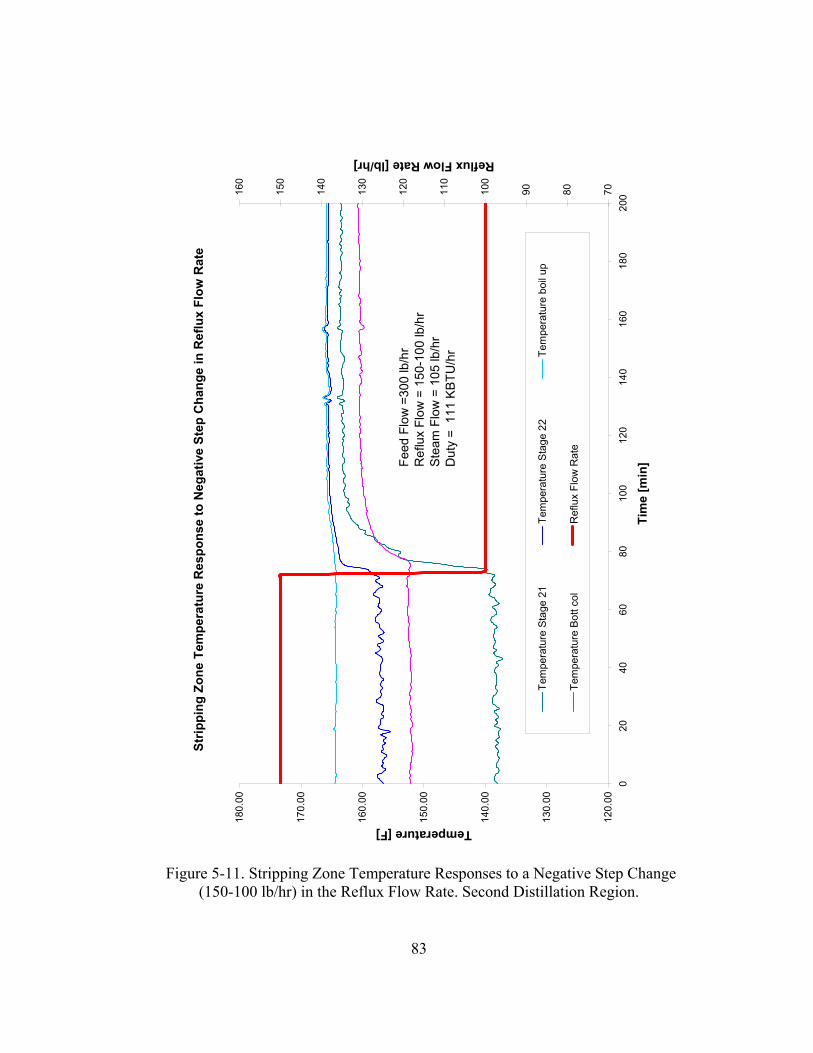
83

Figure 5-11. Stripping Zone Temperature Responses to a Negative Step Change (150-100 lb/hr) in the Reflux Flow Rate. Second Distillation Region.

Strip

ping

Zon

e Te

mpe

ratu

re R

espo

nse

to N

egat

ive

Step

Cha

nge

in R

eflu

x Fl

ow R

ate

120.

00

130.

00

140.

00

150.

00

160.

00

170.

00

180.

00

020

4060

8010

012

014

016

018

020

0

Tim

e [m

in]

Temperature [F]

708090100

110

120

130

140

150

160


Tem

pera

ture

Sta

ge 2

1Te

mpe

ratu

re S

tage

22

Tem

pera

ture

boi

l up

Tem

pera

ture

Bot

t col

Ref

lux

Flow

Rat

e

Feed

Flo

w =

300

lb/h

rR

eflu

x Fl

ow =

150

-100

lb/h

rS

team

Flo

w =

105

lb/h

rD

uty

= 1

11 K

BTU

/hr

84

Figure 5-12. Simulated and Experimental Temperature Responses to a Negative Step Change (150 to100 lb/hr) in the Reflux Flow Rate. Second Distillation Region.

Mod

el T

empe

ratu

re R

espo

nse

Valid

atio

n

80.0

0

90.0

0

100.

00

110.

00

120.

00

130.

00

140.

00

150.

00

160.

00

170.

00

180.

00

020

4060

8010

012

014

016

018

020

0

Tim

e (m

in)

Temperature (F)

90100

110

120

130

140

150

160


Tem

pera

ture

Sta

ge 1

6

Sim

ulat

ion

Tem

pera

ture

Sta

ge 1

6

Tem

pera

ture

Sta

ge 2

2

Sim

ulat

ion

Tem

pera

ture

Sta

ge 2

2

Ref

lux

Flow

Rat

e

Sim

ulat

ion

Ref

lux

Flow

Rat

e

Col

umn

Effic

ienc

y =

0.5

Col

umn

Hea

t Tra

nsfe

r Coe

ffici

ent =

5.5

- 5.5

3 B

TU/h

r*ft2

*F

Feed

Flo

w R

ate

=300

lb/h

rR

eflu

x Fl

ow R

ate

= 15

0-10

0 lb

/hr

Ste

am F

low

Rat

e =

105

lb/h

rR

eboi

ler D

uty

Rat

e =

111

KB

TU/h

r

85

Figure 5-13. Composition Responses to a Negative Step Change (150 to100 lb/hr) in the Reflux Flow Rate. Second Distillation Region.

Com

posi

tion

Res

pons

e to

a N

egat

ive

Step

Cha

nge

in th

e R

eflu

x Fl

ow R

ate

0102030405060708090100

020

4060

8010

012

014

0

Tim

e (m

in)

Composition (wt%)

6080100

120

140

160

180

200


Dis

tilla

te C

5 C

ompo

sitio

n

Botto

m C

6 C

ompo

sitio

n

Botto

m M

eOH

Com

posi

tion

Sim

ulat

ion

Ref

lux

Flow

Rat

e

Dis

tilla

te C

5 co

mpo

sitio

nE

xper

imen

tal

= 76

.09

- 68.

09 w

t%S

imul

ated

= 7

6.56

- 68

.00

wt%

Bot

tom

C6

Com

posi

tion

Exp

erim

enta

l = 1

0.20

- 0.

12 w

t%S

imul

ated

= 1

0.34

- 0.

39 w

t%

Feed

Com

posi

tion

Bef

ore

Ste

p Te

stM

etha

nol =

37.

99 w

t%N

orm

al p

enta

ne =

53.

71 w

t%C

yclo

hexa

ne =

8.3

0 w

t%Fe

ed C

ompo

sitio

n A

fter S

tep

Test

Met

hano

l = 3

6.18

wt%

Nor

mal

pen

tane

= 5

3.89

wt%

Cyc

lohe

xane

= 9

.94

wt%

Bot

tom

MeO

H C

ompo

sitio

n E

xper

imen

tal =

89.

70 -

99.5

7 w

t%S

imul

ated

= 8

9.64

- 99

.29

wt%

86

The reflux step change was performed at a high reboiler duty rate which

moved some of the methanol and all the normal pentane recovery to the top of the

column. These conditions were used to study the columns behavior when the

azeotropic composition is not recovered in the top of the column.

Temperature values decreased with the increase in the reflux flow rate. The

temperature response was not affected by the feed composition disturbance because

the gain is larger in the second region than in the first region.

5.3.2 Changes in reboiler duty rate:

The reboiler duty was manipulated in the experiments by changing the steam

flow rate through the reboiler. The results presented in this section indicate both

steam and duty values.


The results from a negative step change performed in the reboiler duty are

presented below. Temperatures from the rectifying and stripping zones of the column

are presented in Figures 5-14 and 5-15 respectively. Figure 5-16 illustrates a

comparison between the predicted and experimental results and Figure 5-17 shows

the predicted composition profile. Table 5-7 includes a summary of the conditions

before and after the test.

87

Table 5-7. Step change in Reboiler Duty Rate 75 to 68 kBTU/hr. Simulation and Process Results. First Distillation Region.

Before (75 kBTU/hr) After (68 kBTU/hr) FEED DISTILLATE BOTTOM FEED DISTILLATE BOTTOM

Mass Flow [lb/hr] 300.00 147.48 152.52 300.00 143.16 156.84



Cyclohexane 0.4450 0.0020 0.8730 0.4510 0.0020 0.8590



Cyclohexane 0.4452 0.0003 0.8753 0.4540 0.0004 0.8681

88

Figure 5-14. Rectifying Zone Temperature Response to a Negative Step Change (75 to 68 kBTU/hr) in the Reboiler Duty Rate. First Distillation Region.

Rec

tifyi

ng Z

one

Tem

pera

ture

Res

pons

e to

Pos

itive

Ste

p C

hang

e in

Reb

oile

r Dut

y

103

105

107

109

111

113

115

117

020

4060

8010

0

Tim

e [m

in]

Temperature [F]

6065707580859095100

Reboiler Duty [kBTU/hr]

Tem

pera

ture

Ove

rhea

d va

pTe

mpe

ratu

re T

op S

tage

6Te

mpe

ratu

re S

tage

8

Tem

pera

ture

Sta

ge 9

Tem

pera

ture

Sta

ge 1

1Te

mpe

ratu

re S

tage

13

Tem

pera

ture

Sta

ge 1

5Te

mpe

ratu

re S

tage

16

Reb

oile

r Dut

y

Feed

Flo

w =

300

lb/h

rR

eflu

x Fl

ow =

75

lb/h

rS

team

Flo

w =

72.

5-65

lb/h

r

89

Figure 5-15. Stripping Zone Temperature Response to a Negative Step Change (75 to 68 kBTU/hr) in the Reboiler Duty Rate. First Distillation Region.

Strip

ping

Zon

e Te

mpe

ratu

re R

espo

nse

to N

egat

ive

Step

Cha

nge

in R

eboi

ler D

uty

120

130

140

150

160

170

180

020

4060

8010

0

Tim

e [m

in]

Temperature [F]

6065707580859095100


Tem

pera

ture

Sta

ge 2

1Te

mpe

ratu

re S

tage

22

Tem

pera

ture

boi

l up

Tem

pera

ture

Bot

t col

Reb

oile

r Dut

y

Feed

Flo

w =

300

lb/h

rR

eflu

x Fl

ow =

75

lb/h

rS

team

Flo

w =

72.

5-65

lb/h

r

90

Figure 5-16. Simulated and Experimental Temperature Response to a Negative Step Change (75 to 68 kBTU/hr) in the Reboiler Duty Rate. First Distillation Region.

Mod

el T

empe

ratu

re R

espo

nse

Valid

atio

n

6065707580859095100

010

2030

4050

6070

8090

100

Tim

e (m

in)

Reboiler Duty (KBTU/hr)

8090100

110

120

130

140

Temperature (F)

Reb

oile

r Dut

ySi

mul

atio

n R

eboi

ler D

uty

Tem

pera

ture

Sta

ge 1

6Si

mul

atio

n Te

mpe

ratu

re S

tage

16

Tem

pera

ture

Sta

ge 2

2Si

mul

atio

n Te

mpe

ratu

re S

tage

22

Col

umn

Effic

ienc

y =

0.5

Col

umn

Hea

t Tra

nsfe

r Coe

ffici

ent =

5.1

0 B

TU/h

r*ft2

*F

Feed

Flo

w R

ate

=300

lb/h

rR

eflu

x Fl

ow R

ate

= 75

lb/h

rS

team

Flo

w R

ate

= 72

.5-6

5 lb

/hr

Dut

y R

ate

Rat

e =

75-6

8 K

BTU

/hr

91

Figure 5-17. Composition Response to a Negative Step Change (75 to 68 kBTU/hr) in the Reboiler Duty Rate. First Distillation Region.

Com

posi

tion

Res

pons

e to

a N

egat

ive

Step

Cha

nge

in th

e R

eboi

ler D

uty

6065707580859095100

010

2030

4050

6070

8090

100

Tim

e (m

in)

Reboiler Duty (KBTU/hr)

8384858687888990919293

Composition (wt%)

Sim

ulat

ion

Reb

oile

r Dut

yD

istil

late

C5

Com

posi

tion

Botto

m C

6 C

ompo

sitio

n

Dis

tilla

te C

5 co

mpo

sitio

nE

xper

imen

tal

= 91

.70

- 91.

50 w

t%S

imul

ated

= 9

1.91

- 91

.63

wt%

Bot

tom

C6

Com

posi

tion

Exp

erim

enta

l = 8

7.30

- 85

.90

wt%

Sim

ulat

ed =

87.

53 -

86.8

1 w

t%

Feed

Com

posi

tion

Bef

ore

Ste

p Te

stM

etha

nol =

3.9

7 w

t%N

orm

al p

enta

ne =

51.

52 w

t%C

yclo

hexa

ne =

44.

52 w

t%

Feed

Com

posi

tion

Afte

r Ste

p Te

stM

etha

nol =

3.9

9 w

t%N

orm

al p

enta

ne =

50.

61 w

t%C

yclo

hexa

ne =

45.

40 w

t%

Col

umn

Effic

ienc

y =

0.5

Col

umn

Hea

t Tra

nsfe

r Coe

ffici

ent =

5.1

0 B

TU/h

r*ft2

*F

92

The results obtained with the model were very close to the results from the

experiment. The error was less than 1% which is validated by the small material

balance difference in the experimental data. The heat transfer coefficient in the

column was held constant at 5.1 BTU/hr*ft2*F. The efficiency was set at a value of

0.5.


Results from a negative step change in the reboiler duty are presented below.

Figure 5-18 illustrates the temperature results from the column’s rectifying section

and Figure 5-19 illustrates the temperature results from the column’s stripping

section. Figure 5-20 presents a comparison between the predicted and experimental

results and Figure 5-21 shows the predicted composition profile. Table 5-8 includes a

summary of the variable before and after the step test.

Table 5-8. Step change in Reboiler Duty Rate 106 to 61 kBTU/hr. Simulation and Process Results. Second Distillation Region. Before (106 kBTU/hr) After (61 kBTU/hr)

FEED DISTILLATE BOTTOM FEED DISTILLATE BOTTOM

Mass Flow [lb/hr] 300.00 228.53 71.47 300.00 100.12 199.88



Cyclohexane 0.0952 0.1290 0.0069 0.0791 0.0002 0.1221



Cyclohexane 0.0952 0.1249 0.0002 0.0791 0.0052 0.1161

93

Figure 5-18. Rectifying Zone Temperature Responses to a Negative Step Change (106 to 61 kBTU/hr) in the Reboiler Duty Rate. Second Distillation Region.

Rec

tifyi

ng Z

one

Tem

pera

ture

Res

pons

e to

Neg

ativ

e St

ep C

hang

e in

Reb

oile

r Dut

y

100.

0

105.

0

110.

0

115.

0

120.

0

125.

0

020

4060

80

Tim

e [m

in]

Temperature [F]

20.0

40.0

60.0

80.0

100.

0

120.

0

140.

0


Tem

pera

ture

Ove

rhea

d va

pTe

mpe

ratu

re T

op S

tage

6Te

mpe

ratu

re S

tage

8

Tem

pera

ture

Sta

ge 9

Tem

pera

ture

Sta

ge 1

1Te

mpe

ratu

re S

tage

13

Tem

pera

ture

Sta

ge 1

5Te

mpe

ratu

re S

tage

16

Reb

oile

r Dut

y

Feed

Flo

w =

300

lb/h

rR

eflu

x Fl

ow =

100

lb/h

rS

team

Flo

w =

100

-55

lb/h

rD

uty

= 1

06 -

61 K

BTU

/hr

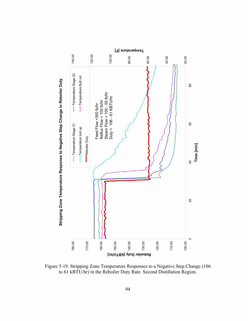
94

Figure 5-19. Stripping Zone Temperature Responses to a Negative Step Change (106 to 61 kBTU/hr) in the Reboiler Duty Rate. Second Distillation Region.

Strip

ping

Zon

e Te

mpe

ratu

re R

espo

nse

to N

egat

ive

Step

Cha

nge

in R

eboi

ler D

uty

100.

00

110.

00

120.

00

130.

00

140.

00

150.

00

160.

00

170.

00

180.

00

020

4060

80

Tim

e [m

in]


20.0

0

40.0

0

60.0

0

80.0

0

100.

00

120.

00

140.

00

Temperature [F]

Tem

pera

ture

Sta

ge 2

1Te

mpe

ratu

re S

tage

22

Tem

pera

ture

boi

l up

Tem

pera

ture

Bot

t col

Reb

oile

r Dut

y Feed

Flo

w =

300

lb/h

rR

eflu

x Fl

ow =

100

lb/h

rS

team

Flo

w =

100

- 55

lb/h

rD

uty

= 1

06 -

61 K

BTU

/hr

95

Figure 5-20. Simulated and Experimental Temperature Responses to a Negative Step Change (106 to 61 kBTU/hr) in the Reboiler Duty Rate. Second Distillation Region.

Mod

el T

empe

ratu

re R

espo

nse

Valid

atio

n

50.0

0

70.0

0

90.0

0

110.

00

130.

00

150.

00

170.

00

020

4060

8010

012

014

0

Tim

e (m

in)

Temperature (F)

0.00

20.0

0

40.0

0

60.0

0

80.0

0

100.

00

120.

00

140.

00

160.

00

180.

00

200.

00

Reboiler Duty (kBTU/hr)

Sim

ulat

ion

Tem

pera

ture

Sta

ge 2

2Te

mpe

ratu

re S

tage

22

Sim

ulat

ion

Tem

pera

ture

Sta

ge 1

6Te

mpe

ratu

re S

tage

16

Sim

ulat

ion

Reb

oile

r Dut

yR

eboi

ler D

uty

Col

umn

Effic

ienc

y =

0.6

Col

umn

Hea

t Tra

nsfe

r Coe

ffici

ent =

5.72

- 5.

63 B

TU/h

r*ft2

*F

Feed

Flo

w R

ate

=300

lb/h

rR

eflu

x Fl

ow R

ate

= 10

0 lb

/hr

Ste

am F

low

Rat

e =

100

- 55

lb/h

rR

eboi

ler D

uty

Rat

e =

106

- 61

KB

TU/h

r

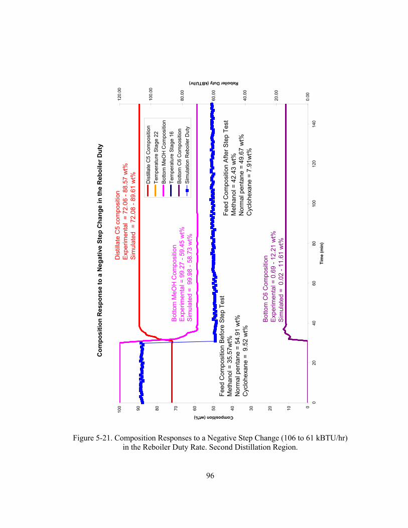
96

Figure 5-21. Composition Responses to a Negative Step Change (106 to 61 kBTU/hr) in the Reboiler Duty Rate. Second Distillation Region.

Com

posi

tion

Res

pons

e to

a N

egat

ive

Step

Cha

nge

in th

e R

eboi

ler D

uty

0102030405060708090100

020

4060

8010

012

014

0

Tim

e (m

in)

Composition (wt%)

0.00

20.0

0

40.0

0

60.0

0

80.0

0

100.

00

120.

00

Reboiler Duty (kBTU/hr)

Dis

tilla

te C

5 C

ompo

sitio

nTe

mpe

ratu

re S

tage

22

Botto

m M

eOH

Com

posi

tion

Tem

pera

ture

Sta

ge 1

6Bo

ttom

C6

Com

posi

tion

Sim

ulat

ion

Reb

oile

r Dut

y

Dis

tilla

te C

5 co

mpo

sitio

nE

xper

imen

tal

= 72

.06

- 88.

57 w

t%S

imul

ated

= 7

2.08

- 89

.61

wt%

Bot

tom

C6

Com

posi

tion

Exp

erim

enta

l = 0

.69

- 12.

21 w

t%S

imul

ated

= 0

.02

- 11.

61 w

t%

Bot

tom

MeO

H C

ompo

sitio

n E

xper

imen

tal =

99.

27 -

59.4

5 w

t%S

imul

ated

= 9

9.98

- 58

.73

wt%

Feed

Com

posi

tion

Bef

ore

Ste

p Te

stM

etha

nol =

35.

57w

t%N

orm

al p

enta

ne =

54.

91 w

t%C

yclo

hexa

ne =

9.5

2 w

t%

Feed

Com

posi

tion

Afte

r Ste

p Te

stM

etha

nol =

42.

43 w

t%N

orm

al p

enta

ne =

49.

67 w

t%C

yclo

hexa

ne =

7.9

1wt%

97

The results from the model gave a close agreement with the results from the

experimental data before the step test was performed. After the change in the reboiler

duty the difference between the predicted and actual data differed in 1% which was

obtained with a constant efficiency value of 0.6. The heat transfer coefficient before

the experiment was 5.72 BTU/hr*ft2*F and decreased with the reboiler duty to 5.63

BTU/hr*ft2*F.

5.3.3 Changes in feed flow rate:


Experimental results for temperatures from the top and bottom of the column

for a negative step change in the feed flow from 300 to 200 lb/hr are plotted in

Figures 5-22 and 5-23 respectively. From these figures, it was observed that the

overhead temperature response had an apparent first order response, and was less

affected by the process noise than were temperatures from the top stages. In the

stripping section temperatures from bottom, boil-up and stage 22 also displayed an

apparent first order response while temperature from stage 21 did not display a

noticeable response to the step change. Simulated and experimental results for

temperatures from stages 16 and 22 are presented in Figure 5-24. The composition

response from the model is presented in Figure 5-25. The heat transfer coefficient

before the step change was 6.1 BTU/hr*ft2*F and decreased to 5.6 BTU/hr*ft2*F

98

after the feed flow was reduced. The predicted composition before the step change

was the same composition given by the experiment but the composition after the step

test was off by 2%. The column efficiency was maintained at 0.7 to match the

simulated distillate composition with the experimental value. The difference between

the experiment and the model could be explained by the error in the measurement as

indicated by the material balance difference in the experiment.

Table 5-9. Step change in Feed Flow Rate 300 to 200 lb/hr. Simulation and Process Results. First Distillation Region. Before (300 lb/hr) After (200 lb/hr)

FEED DISTILLATE BOTTOM FEED DISTILLATE BOTTOM

Mass Flow [lb/hr] 300.00 86.78 213.22 200.00 81.90 118.10



Cyclohexane 0.5430 0.0028 0.7679 0.4864 0.0019 0.8322



Cyclohexane 0.5430 0.0011 0.7636 0.4864 0.0003 0.8234

99

Figure 5-22. Rectifying Zone Temperature Responses to a Negative Step Change (300 to 200 lb/hr) in the Feed Flow Rate. First Distillation Region.

Rec

tifyi

ng Z

one

Tem

pera

ture

Res

pons

e to

Neg

ativ

e St

ep C

hang

e in

Fee

d Fl

ow R

ate

100

105

110

115

120

125

020

4060

8010

012

014

0

Tim

e [m

in]

Temperature [F]

150

170

190

210

230

250

270

290

310

330

350

Feed Flow Rate [lb/hr]

Tem

pera

ture

Ove

rhea

d va

pTe

mpe

ratu

re T

op S

tage

6Te

mpe

ratu

re S

tage

8

Tem

pera

ture

Sta

ge 9

Tem

pera

ture

Sta

ge 1

1Te

mpe

ratu

re S

tage

13

Tem

pera

ture

Sta

ge 1

5Te

mpe

ratu

re S

tage

16

Feed

Flo

w R

ate

Feed

Flo

w =

300-

200

lb/h

rR

eflu

x Fl

ow =

110

lb/h

rS

team

Flo

w =

65

lb/h

rR

eboi

ler D

uty

= 69

kB

TU/h

r

100

Figure 5-23. Stripping Zone Temperature Responses to a Negative Step Change (300 to 200 lb/hr) in the Feed Flow Rate. First Distillation Region.

Strip

ping

Zon

e Te

mpe

ratu

re R

espo

nse

to N

egat

ive

Step

Cha

nge

in F

eed

Flow

Rat

e

120

130

140

150

160

170

180

190

020

4060

8010

012

014

0

Tim

e [m

in]

Temperature [F]

150

170

190

210

230

250

270

290

310

330

350


Tem

pera

ture

Sta

ge 2

1Te

mpe

ratu

re S

tage

22

Tem

pera

ture

boi

l up

Tem

pera

ture

Bot

t col

Feed

Flo

w R

ate

Feed

Flo

w =

300-

200

lb/h

rR

eflu

x Fl

ow =

110

lb/h

rS

team

Flo

w =

65

lb/h

rR

eboi

ler D

uty

= 69

kB

TU/h

r

101

Figure 5-24. Simulated and Experimental Temperature Responses to a Negative Step Change (300 to 200 lb/hr) in the Feed Flow Rate. First Distillation Region.

Mod

el T

empe

ratu

re R

espo

nse

Valid

atio

n

150

170

190

210

230

250

270

290

310

330

350

010

2030

4050

6070

8090

100

Tim

e (m

in)

Feed Flow Rate (lb/hr)

8090100

110

120

130

140

150

160

170

Temperature (F)

Feed

Flo

w R

ate

Sim

ulat

ion

Feed

Flo

w R

ate

Tem

pera

ture

Sta

ge 1

6Si

mul

atio

n Te

mpe

ratu

re S

tage

16

Tem

pera

ture

Sta

ge 2

2Si

mul

atio

n Te

mpe

ratu

re S

tage

22

Col

umn

Effic

ienc

y =

0.7

Col

umn

Hea

t Tra

nsfe

r Coe

ffici

ent =

6.1

- 5.

96 B

TU/h

r*ft2

*F

Feed

Flo

w R

ate

=300

-200

lb/h

rR

eflu

x Fl

ow R

ate

= 11

0 lb

/hr

Ste

am F

low

Rat

e =

65 lb

/hr

Reb

oile

r Dut

y R

ate

= 69

kB

TU/h

r

102

Figure 5-25. Composition Response to a Negative Step Change (300 to 200 lb/hr) in the Feed Flow Rate. First Distillation Region.

Com

posi

tion

Res

pons

e to

a N

egat

ive

Step

Cha

nge

in th

e Fe

ed F

low

Rat

e

150

170

190

210

230

250

270

290

310

330

350

010

2030

4050

6070

8090

100

Tim

e (m

in)


707580859095

Composition (wt%)

Sim

ulat

ion

Feed

Flo

w R

ate

Dis

tilla

te C

5 C

ompo

sitio

nBo

ttom

C6

Com

posi

tion

Dis

tilla

te C

5 co

mpo

sitio

nE

xper

imen

tal

= 91

.26

- 94.

61 w

t%S

imul

ated

= 9

1.26

- 92

.39

wt%

Bot

tom

C6

Com

posi

tion

Exp

erim

enta

l = 7

6.79

- 83

.22

wt%

Sim

ulat

ed =

76.

36 -

82.3

4 w

t%

Feed

Com

posi

tion

Bef

ore

Ste

p Te

stM

etha

nol =

3.1

3 w

t%N

orm

al p

enta

ne =

42.

56 w

t%C

yclo

hexa

ne =

54.

30 w

t%

Feed

Com

posi

tion

Afte

r Ste

p Te

stM

etha

nol =

3.1

1 w

t%N

orm

al p

enta

ne =

48.

26 w

t%C

yclo

hexa

ne =

48.

64 w

t%Fe

ed F

low

Rat

e =3

00-2

00 lb

/hr

Ref

lux

Flow

Rat

e =

110

lb/h

rS

team

Flo

w R

ate

= 65

lb/h

rR

eboi

ler D

uty

Rat

e =

69 k

BTU

/hr

103


Experimental results for temperatures from rectifying and stripping sections

for a negative step change in the feed flow from 300 to 200 lb/hr are plotted in

Figures 5-26 and 5-27 respectively. Simulated results for the temperatures from

stages 16 and 22 are compared with the experimental values in Figure 5-28. Figure

5-29 presents the simulation composition response. Table 5-10 summarizes the results

from the experiment and the simulation before and after the step change.

Table 5-10. Step change in Feed Flow Rate 300 to 200 lb/hr. Simulation and Process Results. Before (300 lb/hr) After (200 lb/hr)

FEED DISTILLATE BOTTOM FEED DISTILLATE BOTTOM Mass Flow

[lb/hr] 300.00 115.41 184.59 200.00 109.59 90.41



Cyclohexane 0.0957 0.0002 0.1419 0.0920 0.0004 0.1823



Cyclohexane 0.0957 0.0077 0.1507 0.0912 0.0161 0.1823

The heat transfer coefficient before the step test was 5.72 kBTU/hr and

increased with the decrease in feed flow to 5.80 kBTU/hr. The efficiency was

maintained constant at 0.5 during the test.

104

Figure 5-26. Rectifying Zone Temperature Responses to a Negative Step Change (300 to 200 lb/hr) in the Feed Flow Rate. Second Distillation Region.

Rec

tifyi

ng Z

one

Tem

pera

ture

Res

pons

e to

a N

egat

ive

Step

Cha

nge

in F

eed

Flow

Rat

e

102.

00

102.

50

103.

00

103.

50

104.

00

104.

50

105.

00

105.

50

106.

00

106.

50

107.

00

020

4060

8010

012

014

016

018

020

022

024

026

028

030

0

Tim

e [m

in]

Temperature [F]

150

200

250

300

350

400


Tem

pera

ture

Ove

rhea

d va

pTe

mpe

ratu

re T

op S

tage

6Te

mpe

ratu

re S

tage

9

Tem

pera

ture

Sta

ge 1

1Te

mpe

ratu

re S

tage

13

Tem

pera

ture

Sta

ge 1

5

Tem

pera

ture

Sta

ge 1

6Fe

ed F

low

Rat

eTe

mpe

ratu

re S

tage

8

Feed

Flo

w R

ate

=300

-200

lb/h

rR

eflu

x Fl

ow R

ate

= 10

0 lb

/hr

Ste

am F

low

Rat

e =

58 lb

/hr

Dut

y R

ate

= 6

3 K

BTU

/hr

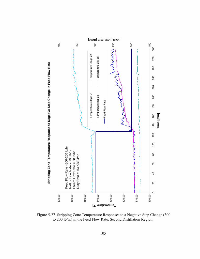
105

Figure 5-27. Stripping Zone Temperature Responses to a Negative Step Change (300 to 200 lb/hr) in the Feed Flow Rate. Second Distillation Region.

Strip

ping

Zon

e Te

mpe

ratu

re R

espo

nse

to N

egat

ive

Step

Cha

nge

in F

eed

Flow

Rat

e

100.

00

110.

00

120.

00

130.

00

140.

00

150.

00

160.

00

170.

00

020

4060

8010

012

014

016

018

020

022

024

026

028

030

0

Tim

e [m

in]

Temperature [F]

150

200

250

300

350

400


Tem

pera

ture

Sta

ge 2

1Te

mpe

ratu

re S

tage

22

Tem

pera

ture

boi

l up

Tem

pera

ture

Bot

t col

Feed

Flo

w R

ate

Feed

Flo

w R

ate

=300

-200

lb/h

rR

eflu

x Fl

ow R

ate

= 10

0 lb

/hr

Ste

am F

low

Rat

e =

58 lb

/hr

Dut

y R

ate

= 6

3 K

BTU

/hr

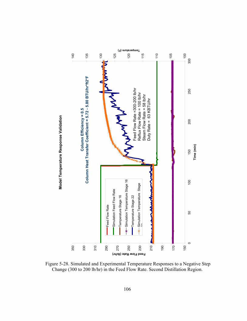
106

Figure 5-28. Simulated and Experimental Temperature Responses to a Negative Step Change (300 to 200 lb/hr) in the Feed Flow Rate. Second Distillation Region.

Mod

el T

empe

ratu

re R

espo

nse

Valid

atio

n

150

170

190

210

230

250

270

290

310

330

350

050

100

150

200

250

300

Tim

e (m

in)


100

105

110

115

120

125

130

135

140

Temperature (F)

Feed

Flo

w R

ate

Sim

ulat

ion

Feed

Flo

w R

ate

Tem

pera

ture

Sta

ge 1

6

Sim

ulat

ion

Tem

pera

ture

Sta

ge 1

6

Tem

pera

ture

Sta

ge 2

2

Sim

ulat

ion

Tem

pera

ture

Sta

ge22

Feed

Flo

w R

ate

=300

-200

lb/h

rR

eflu

x Fl

ow R

ate

= 10

0 lb

/hr

Ste

am F

low

Rat

e =

58 lb

/hr

Dut

y R

ate

= 6

3 K

BTU

/hr

Col

umn

Effic

ienc

y =

0.5

Col

umn

Hea

t Tra

nsfe

r Coe

ffici

ent =

5.7

2 - 5

.80

BTU

/hr*

ft2*F

107

Figure 5-29. Composition Response to a Negative Step Change (300 to 200 lb/hr) in the Feed Flow Rate. Second Distillation Region.

Com

posi

tion

Res

pons

e to

a N

egat

ive

Step

Cha

nge

in th

e Fe

ed F

low

Rat

e

150

170

190

210

230

250

270

290

310

330

350

050

100

150

200

250

300

Tim

e (m

in)


0102030405060708090100

Composition (wt%)

Sim

ulat

ion

Feed

Flo

w R

ate

Dis

tilla

te C

5 C

ompo

sitio

n

Botto

m C

6 C

ompo

sitio

n

Botto

m M

eOH

Com

posi

tion

Dis

tilla

te C

5 co

mpo

sitio

nE

xper

imen

tal

= 86

.55

- 86.

31 w

t%S

imul

ated

= 8

9.08

. - 8

7.41

wt%

Bot

tom

C6

Com

posi

tion

Exp

erim

enta

l = 1

4.19

- 18

.23

wt%

Sim

ulat

ed =

15.

02 -

18.2

7 w

t%

Feed

Com

posi

tion

Bef

ore

Ste

p Te

stM

etha

nol =

39.

28 w

t%N

orm

al p

enta

ne =

51.

16 w

t%C

yclo

hexa

ne =

9.5

7 w

t%Fe

ed C

ompo

sitio

n A

fter S

tep

Test

Met

hano

l = 3

9.20

wt%

Nor

mal

pen

tane

= 5

1.60

wt%

Cyc

lohe

xane

= 9

.12

wt%

Bot

tom

MeO

H C

ompo

sitio

n E

xper

imen

tal =

57.

35 -7

1.57

wt%

Sim

ulat

ed =

57.

53 -

73.5

5 w

t%

Feed

Flo

w R

ate

=300

-200

lb/h

rR

eflu

x Fl

ow R

ate

= 10

0 lb

/hr

Ste

am F

low

Rat

e =

58 lb

/hr

Dut

y R

ate

= 6

3 K

BTU

/hr

108

Although the responses in both distillation regions were symmetric for the

negative step changes in the feed flow, the top temperatures in the second region

increased when feed flow decreased but the gain was one order of magnitude smaller

than the gain in the first region. It was observed in both regions that the feed

temperature was disturbed with feed flow changes but the controller responded fast to

bring the temperature value back to the set point.

Temperatures from the very bottom in the second distillation region responded

with longer time constant than temperatures from the middle. Temperatures from

stages 15 and 16 were held almost constant. Compared with the first distillation

region, temperatures below stage 21 responded with higher gain to changes in the

feed flow in the second distillation region.

5.3.4 Feed Composition Step Test

A feed composition step test, which changed the operation from the second

distillation region (feed composition rich in methanol) to the first distillation region

(feed composition rich in cyclohexane), was performed in the experimental system

and the results used to validate the model dynamic predictions. The results from the

test and the predictions given by the simulation are presented in this section. Figure

5-30 illustrates the model validation using the temperature responses from the

experimental data and Figure 5-31 presents the predicted composition profile

obtained from the simulation.

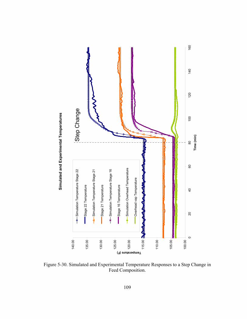
109

Figure 5-30. Simulated and Experimental Temperature Responses to a Step Change in Feed Composition.

Sim

ulat

ed a

nd E

xper

imen

tal T

empe

ratu

res

100.

00

105.

00

110.

00

115.

00

120.

00

125.

00

130.

00

135.

00

140.

00

020

4060

8010

012

014

016

0

Tim

e (m

in)

Temperature (F)

Sim

ulat

ion

Tem

pera

ture

Sta

ge 2

2

Stag

e 22

Tem

pera

ture

Sim

ulat

ion

Tem

pera

ture

Sta

ge 2

1

Stag

e 21

Tem

pera

ture

Sim

ulat

ion

Tem

pera

ture

Sta

ge 1

6

Stag

e 16

Tem

pera

ture

Sim

ulat

ion

Ove

rhea

d Te

mpe

ratu

re

Ove

rhea

d va

p Te

mpe

ratu

re

Step

Cha

nge

110

Figure 5-31. Composition Responses to a Step Change in Feed Composition.

Mod

el C

ompo

sitio

ns

0102030405060708090100

020

4060

8010

012

014

016

0

Tim

e (m

in)

Composition (Wt %)

MeO

H D

istil

late

Com

posi

tion

C5

Dis

tilla

te C

ompo

sitio

nC

6 D

istil

late

Com

posi

tion

MeO

H B

otto

m C

ompo

sitio

nC

5 Bo

ttom

Com

posi

tion

C6

Botto

m C

ompo

sitio

nM

eOH

Fee

d C

ompo

sitio

nC

5 Fe

ed C

ompo

sitio

nC

6 Fe

ed C

ompo

sitio

n

Ste

p C

hang

e

Exp

erim

enta

l Com

posi

tions

Bef

ore

Step

Tes

t.:

Dis

tilla

te:

MEO

H =

11.

250

C5

= 88

.682

C

6 =

0.06

8

Botto

mM

EOH

= 6

1.90

4 C

5 =

20.9

93

C6

= 17

.103

Feed

: M

EOH

= 4

1.43

1 C

5 =

48.5

19

C6

= 10

.05

Expe

rimen

tal C

ompo

sitio

ns A

fter S

tep

Test

.:

Dis

tilla

te:

MEO

H =

10.

664

C5

= 86

.151

C

6 =

3.15

4

Botto

mM

EOH

= 0

.882

C

5 =

18.1

7 C

6 =

80.9

48

Feed

: M

EOH

= 3

.55

C5

= 36

.711

C

6 =

59.7

39

Hea

t tra

nsfe

r coe

ffici

ent:

Befo

re: 7

.65

Afte

r: 8.

65

111

From the results it was observed that the model closely followed the experimental

data. The temperatures in the model followed the experimental data and the dynamic

response gave very good agreement, having very similar gains and time constants.

The composition predicted by the model was also accurate; however there was an

important difference in the time constants. The model reached the compositions

steady state values faster than the experiment.

5.4 Summary and Discussion

A dynamic simulation of an azeotropic distillation system was carried out and

the results compared with experimental data from a real plant. The model developed

was an equilibrium model. Although the results at steady state, before and after each

step change, had very good agreement with the experimental data, the model transient

response did not always follow the experimental transient response. This effect might

be a result of the equilibrium assumption, which is not a valid assumption when the

system is not at steady state.

Two model parameters, column’s heat transfer coefficient and dynamic

efficiency, were modified to match the model and experiment results. It was

concluded that the column behavior in each distillation region is different. This

behavior is produced by the different interactions between the system components.

Since the distillation regions have demonstrated a very different behavior among

112

them, each region could be considered as a separate system for operation and control

purposes.

The heat transfer coefficient is a good parameter to perform model

reconciliation, because by directly modifying the heat loss in the column adjusts the

material balance in the system. The efficiency in the column also demonstrated to be

a good parameter to fit the model with the experimental data. However, for this

particular system, where the error in the measurements is comparable with the range

of change in the output parameter, it may give the same result to keep the parameter

at a constant value. Based on the results from this work, it is concluded that the

efficiency is a very good parameter to perform model reconciliation in systems with

an accurate and fast measurement of composition.

The temperatures did not change significantly after the step changes were

performed while the compositions did. This behavior impedes the use of temperature

measurements as control variables; therefore other alternatives must be considered.

113

Chapter 6. Online Model Reconciliation and Control

Azeotropic distillation processes display a highly non-ideal behavior which, as

presented in previous chapters, is also reflected in their nonlinear dynamic responses.

Except for some studies that used PID controllers where the control structure does not

follow traditional distillation schemes, azeotropic distillation has been usually

controlled with similar configurations as ordinary distillation. A literature review of

control of azeotropic distillation was included in Chapter 2. In the absence of online

measurements of composition, temperature is the variable of choice for controlling

the separation in a distillation column. However, composition of multicomponent,

non-ideal mixtures can not be inferred only based on temperature measurements. This

chapter describes an online model reconciliation technique used to minimize the error

between the process and the model predictions. The model is used to obtain an

inferential control solution for control schemes for azeotropic distillation using PID

and model-based control algorithms.

6.1 Model Reconciliation Approach

Traditionally, model reconciliation is performed using a steady-state model and

the parameter estimates are obtained offline using an optimization algorithm, such as

the weighted least square (WLS) formulation, where the objective is to find estimates

114

that minimize the squared error in the measurements, normalized by the measurement

covariance. Usually before the parameters are estimated, the measurement data are

first validated with some conservation equations, and then adjusted such that the

model parameters and the adjusted data satisfy the process model equations.

Although the present work approach uses a reconciliation module to calculate

the model parameters that minimize the error between plant measurement and model

variables, it is not based on a traditional data reconciliation / parameter estimation

configuration. The method tunes a dynamic model seeking to match data from the

process while using traditional blocks presented in a process control software for a

computer control system.

a)

115

b)

Figure 6-1. a) Block diagram of a model-reference adaptive system. b) Block diagram of the current model reconciliation approach.

The algorithm used in the reconciliation module is based on the gradient

approach for model-reference adaptive control [2]. The objective is to modify the

parameters in the model so that the error between the outputs of process and reference

model is driven to zero (see Figure 6.1.a). In the gradient approach the parameter is

obtained as the output of an integrator. A potentially quicker adaptation could also be

achieved by adding a proportional adjustment to the integral action. The control law

then takes the form of (6-1), which can be implemented in the plant using PI

controller software where the constants 1γ and 2γ represent the proportional and

integral gains respectively [2].

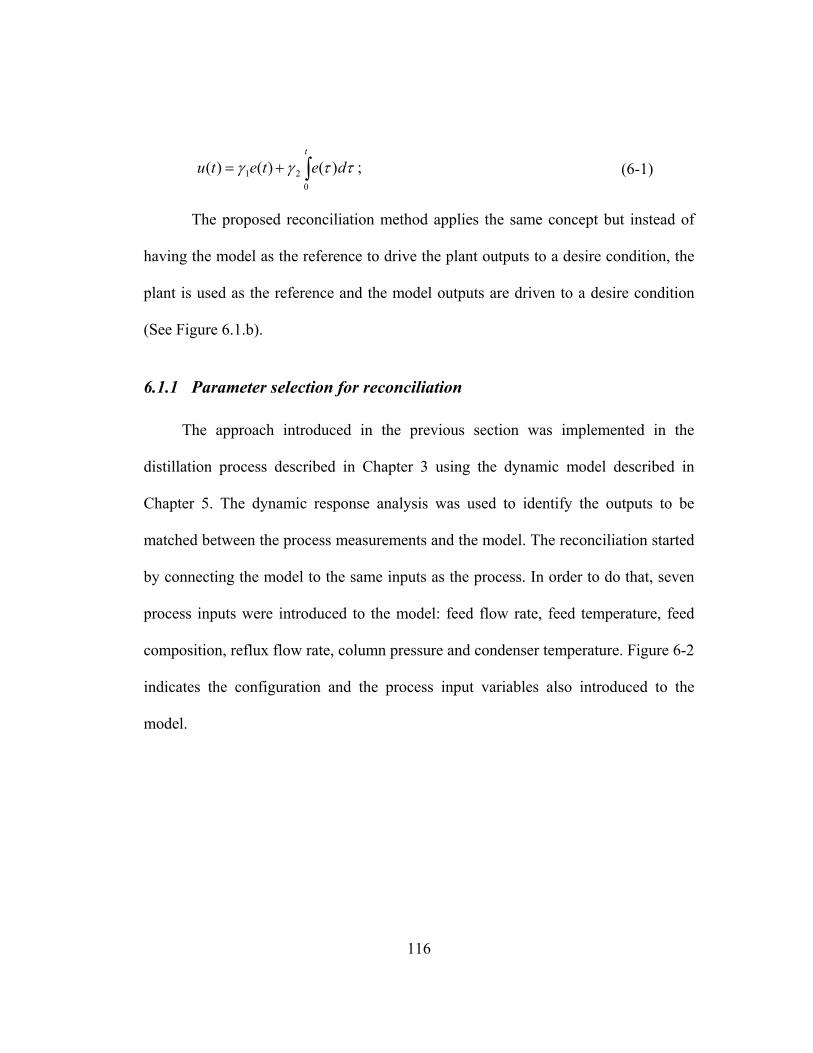
116

∫+=t

detetu0

21 )()()( ττγγ ; (6-1)

The proposed reconciliation method applies the same concept but instead of

having the model as the reference to drive the plant outputs to a desire condition, the

plant is used as the reference and the model outputs are driven to a desire condition

(See Figure 6.1.b).

6.1.1 Parameter selection for reconciliation

The approach introduced in the previous section was implemented in the

distillation process described in Chapter 3 using the dynamic model described in

Chapter 5. The dynamic response analysis was used to identify the outputs to be

matched between the process measurements and the model. The reconciliation started

by connecting the model to the same inputs as the process. In order to do that, seven

process inputs were introduced to the model: feed flow rate, feed temperature, feed

composition, reflux flow rate, column pressure and condenser temperature. Figure 6-2

indicates the configuration and the process input variables also introduced to the

model.

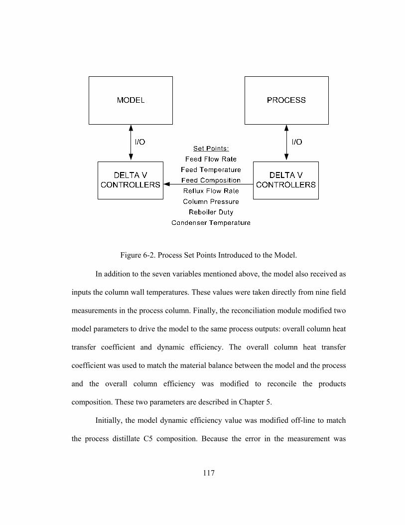
117

Figure 6-2. Process Set Points Introduced to the Model.

In addition to the seven variables mentioned above, the model also received as

inputs the column wall temperatures. These values were taken directly from nine field

measurements in the process column. Finally, the reconciliation module modified two

model parameters to drive the model to the same process outputs: overall column heat

transfer coefficient and dynamic efficiency. The overall column heat transfer

coefficient was used to match the material balance between the model and the process

and the overall column efficiency was modified to reconcile the products

composition. These two parameters are described in Chapter 5.

Initially, the model dynamic efficiency value was modified off-line to match

the process distillate C5 composition. Because the error in the measurement was

118

about 3%, the parameter was modified if the model output was off by more than 3%

from the process output. After data from the experiments were analyzed, it was

concluded that the efficiency value was best described by value of 0.7 in the

distillation region rich in cyclohexane and pentane and 0.5 in the distillation region

rich in methanol and normal pentane.

The column’s heat transfer coefficient directly influences the heat loss

experienced by the column. The model developed in this work used a simple heat loss

model described by Equation (5-3). The heat transfer coefficient was updated online

using the reconciliation module during the control experiments described in this

chapter. Its value increased up to 5% as the liquid flow in the column decreased and

vice versa. The heat transfer coefficient depends on the physical properties of the

fluid and the physical conditions of the experiment. As both fluid composition and

process conditions changed with the operation region, the heat transfer coefficient

also changed. In addition, the heat transfer coefficient reflects the variations in the

ambient temperature given that this value was not measured continuously nor

automatically upgraded during the experiments. Although, this variation was found to

be small, it shifted the model from the process outputs.

Since there was not an online measurement of composition, the reconciliation

module was only used online to modify the efficiency value during steady state

conditions, after the process samples were analyzed. The heat transfer coefficient was

continuously modified during the dynamic changes and reached a constant value at

119

steady state conditions. The average heat transfer coefficient value in the first

distillation region was 5.7 BTU/hr*ft2*F and 5.6 BTU/hr*ft2*F in the second

distillation region.

6.1.2 Implementation results During the experiments the model was set to follow the process set points

from the variables illustrated in Figure 6-3.

0

20

40

60

80

100

120

140

160

180

200

220

240

260

280

300

0 50 100 150 200

Time (min)

Flow

Rat

e (lb

/hr)

/ R

eboi

ler D

uty

(kB

TU/h

r)

Reboiler Duty Simulation Reboiler Duty

Feed Temperature Simulation Feed Temperature

Overhead Liquid Temperature Simulation Overhead Liquid Temperature

Reflux Flow Simulation Reflux Flow

Column Pressure Simulation Column Pressure

Feed Flow Simulation Feed Flow

Figure 6-3. Model Outputs Determined by the Process Set Points.

During the dynamic model validation presented in Chapter 5 it was observed

that different combinations of heat transfer coefficient and dynamic efficiency values

gave the same combination of composition and material balance in the column.

120

Although there should be a unique minimum in the squared error, the final parameter

values were influenced by the module initial conditions. It was determined that

limiting the parameter values to a tight range around the average value did not always

force the parameter values to their desired values. For these reasons the reconciliation

module algorithm was modified to perform the parameter reconciliation using a batch

data approach rather than a sequential approach. First the heat transfer coefficient was

modified until the model material balance was reconciled with the process data and

then the dynamic efficiency value was modified if necessary to obtain the desire

composition in the distillate stream. Figure 6-4 illustrates the approach. The operation

of each reconciliation module was determined by the logic block presented in Figure

6-5. The block works as follow: The error signal (e1(t)) from the material balance

activates module 1 through an AND gate (Gate 1) which drives the error to zero. The

other input to Gate 1 is the negation of the status of module 2; this assures that

module 1 is not activated while module 2 is active. After the material balance is

reconciled, module 2 is activated through Gate 2 which reconciles the composition in

the distillate stream. Module 2 is not activated if module 1 is active. After the

distillate composition is reconcile, module 1 could be activated again if necessary,

that is, if the material balance error is different from zero and the cycle starts again.

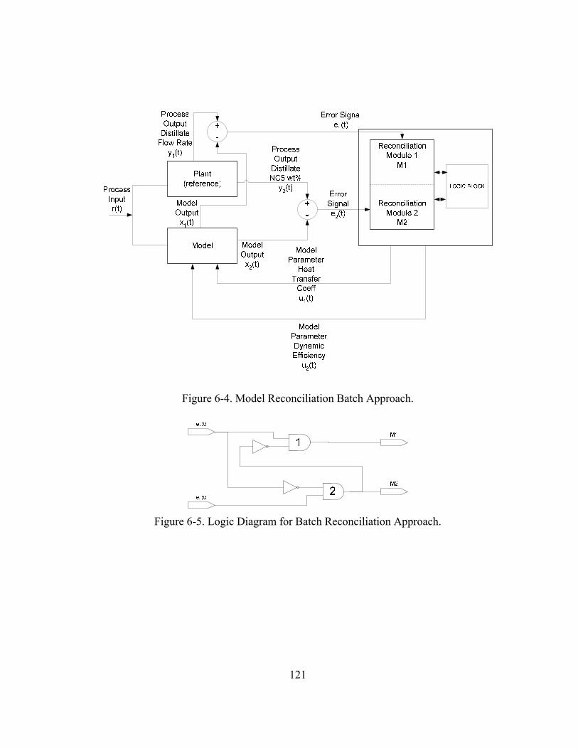
121

Figure 6-4. Model Reconciliation Batch Approach.

Figure 6-5. Logic Diagram for Batch Reconciliation Approach.

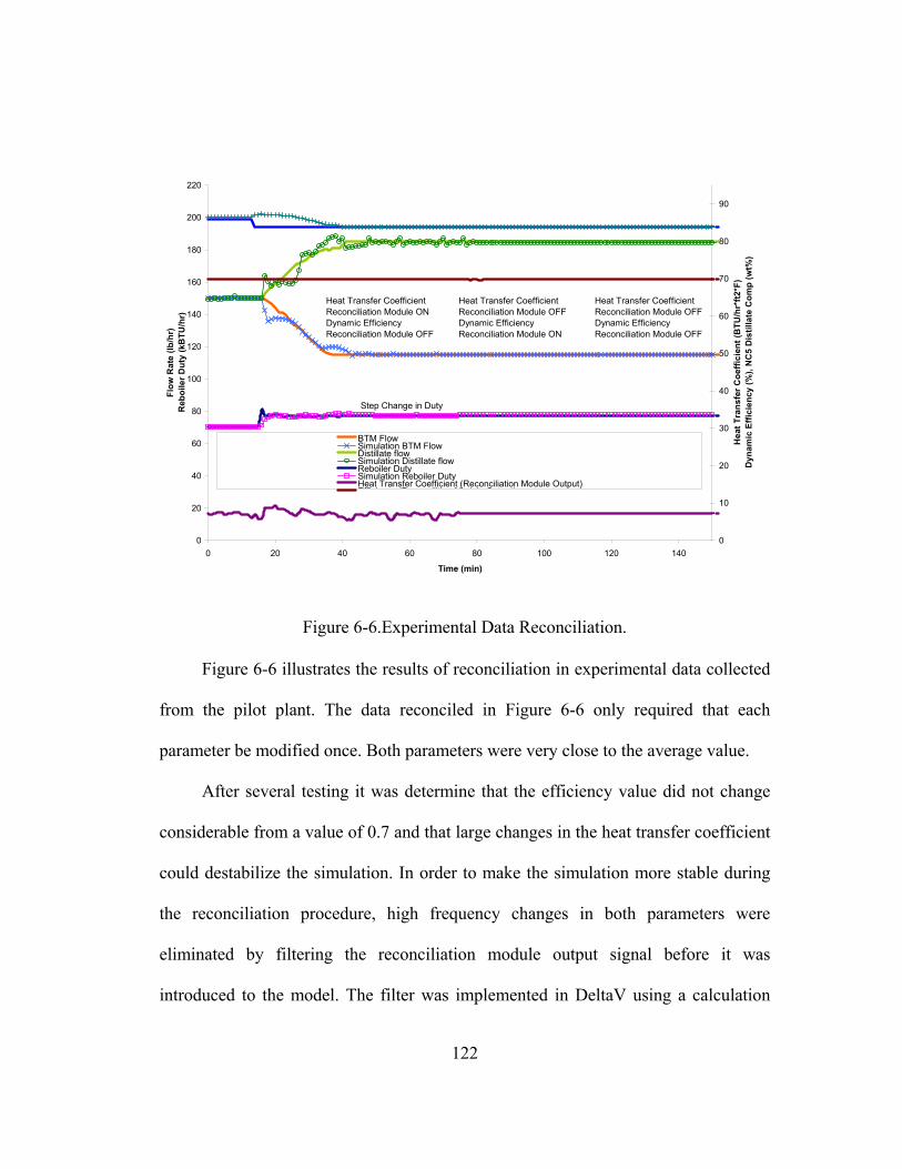
122

0

20

40

60

80

100

120

140

160

180

200

220

0 20 40 60 80 100 120 140

Time (min)

Flow

Rat

e (lb

/hr)

R

eboi

ler D

uty

(kB

TU/h

r)

0

10

20

30

40

50

60

70

80

90

Hea

t Tra

nsfe

r Coe

ffici

ent (

BTU

/hr*

ft2*F

)D

ynam

ic E

ffici

ency

(%),

NC

5 D

istil

late

Com

p (w

t%)

BTM FlowSimulation BTM FlowDistillate flowSimulation Distillate flowReboiler DutySimulation Reboiler DutyHeat Transfer Coefficient (Reconciliation Module Output)Effi i (R iliti M d l O t t)

Heat Transfer Coefficient Reconciliation Module ONDynamic Efficiency Reconciliation Module OFF

Step Change in Duty

Heat Transfer Coefficient Reconciliation Module OFFDynamic Efficiency Reconciliation Module ON

Heat Transfer Coefficient Reconciliation Module OFFDynamic Efficiency Reconciliation Module OFF

Figure 6-6.Experimental Data Reconciliation.

Figure 6-6 illustrates the results of reconciliation in experimental data collected

from the pilot plant. The data reconciled in Figure 6-6 only required that each

parameter be modified once. Both parameters were very close to the average value.

After several testing it was determine that the efficiency value did not change

considerable from a value of 0.7 and that large changes in the heat transfer coefficient

could destabilize the simulation. In order to make the simulation more stable during

the reconciliation procedure, high frequency changes in both parameters were

eliminated by filtering the reconciliation module output signal before it was

introduced to the model. The filter was implemented in DeltaV using a calculation

123

block that calculated and upgraded the parameter’s average value during time

intervals of two minutes. Each variable was sampled every second in DeltaV.

Figure 6-7 illustrates the results from model reconciliation with experimental

data, during the reconciliation the heat transfer coefficient was modified while the

dynamic efficiency was maintained at 0.7.

0

20

40

60

80

100

120

140

160

180

200

220

0 50 100 150 200 250

Time (min)

Flow

Rat

e (lb

/hr)

0

2

4

6

8

10

12

14

Hea

t Tra

nsfe

r Coe

ffici

ent (

BTU

/hr*

ft2*F

)

Experiment SP BTM Flow RateSimulation BTM Flow RateExperiment SP Distillate Flow RateSimulation Distillate Flow RateHeat Transfer Coefficient (Reconciliation Module Output)

Heat Transfer Coefficient Reconciliation Module ONDynamic Efficiency = 0.7

Heat Transfer Coefficient Reconciliation Module ONDynamic Efficiency = 0.7

Heat Transfer Coefficient Reconciliation Module OFF

Heat Transfer Coefficient Reconciliation Module OFF

Average ambient temperature 100 F Average ambient temperature 68 F

Figure 6-7.Experimental Data Reconciliation Filtering the Heat Transfer Coefficient Signal.

The experimental data used in Figure 6-7 was collected from two experiments

performed under different ambient conditions using a feed composition from the first

distillation region. Data from 0 to 150 min was collected during the summer where

124

the ambient temperature reached 100 F; the heat transfer coefficient during these

conditions was close to 5 Btu/hr*ft2*F. The first part of the plot (time 0 to 50 min)

illustrates the model behavior before the reconciliation module was turned ON. The

initial heat transfer coefficient value was set arbitrary at 9.8 Btu/hr*ft2*F. In this time

interval, the model distillate flow rate is 120 lb/hr while the experiment distillate flow

rate is 140 lb/hr. This means that the heat loss in the model is larger than the heat loss

in the process and the heat transfer coefficient value should be smaller. At time 50

min the reconciliation module is turned ON and the heat transfer coefficient is

decreased by the module to a steady state value of 4.8 Btu/hr*ft2*F. The filter in the

parameter estimation eliminated the oscillation after the change at time 65 min.

Before the filter was implemented, it was necessary to have a good initial guess for

the parameter value. The filter introduced a delay in the reconciliation module

response; this delay is proportional to the difference between the parameter’s initial

guess and final value. The second set of data (150 to 250 min) was collected with

average ambient temperature of 68 F. The initial heat transfer coefficient value was

set to 5 Btu/hr*ft2*F, which was close to the final value found with the reconciliation

module. The heat transfer coefficient at t=250 min was close to 6 Btu/hr*ft2*F. It was

observed that the reconciliation module followed very well the experimental data in

both data sets.

125

6.2 Controllability Analysis

Composition inferred by temperature measurements is a common practice in

distillation control. Although temperature has been the measurement of choice in

monitoring and controlling the separation due to its fast response and low cost, for

highly non-ideal systems holding the temperature constant does not imply that

composition will also be constant. In such cases direct measurements of composition

using online analyzers should be considered. However, online analyzers involve high

capital and maintenance cost and slow response, especially for multiplexed sample

points. In order to overcome these issues, this work introduced the use of a high

fidelity dynamic model as a soft sensor for product composition.

The process control strategy was configured in two levels:

1) Stabilize the basic operation of the column. This included inventory (level), flow

and pressure controls. The control loops in this level (see Table 6-1) were configured

with independent PID controllers.

Table 6-1. Basic Operation Process Variables

Manipulated Variable Controlled Variables Feed Flow Valve Position Feed Flow Rate Preheater Steam Flow Valve Position Feed Temperature Reflux Flow Valve Position Reflux Flow Rate Distillate Flow Valve Position Distillate Flow Rate Bottom Flow Valve Position Bottom Flow Rate Reboiler Steam Flow Valve Position Steam Flow Rate / Reboiler Duty Rate Nitrogen Flow Splitter Valve Position Column Pressure

126

In addition to the variables listed above, there were two controlled variables

that correspond to the first control level, accumulator and column bottom hold-up.

Their corresponding manipulated variables were selected among distillate, reflux,

steam, and bottom flow rates.

2) Control the product composition in the column. Two different configurations were

considered for this level. These configurations were selected based on the relative

gain array analysis (RGA).

6.2.1 Pairing of Controlled and manipulated variables

Although the relative gain array (RGA) method is a steady state analysis

based on a linearized system, it was used to pair variables in the inventory and

separation control. The gain matrix was calculated using the results from the dynamic

model developed in HYSYS. Different step changes were performed in the

manipulated variables, using different magnitudes and directions and finally the

results were averaged. These results are summarized in Table 6-2. The controlled

variables are normal pentane distillate composition (DC) and cyclohexane bottom

composition (BC). The possible manipulated variables are distillate, reflux, bottom,

and steam flow rate. The results of pairing manipulated and controlled variables using

the RGA method is summarized in Table 6-3.

127

Table 6-2. Gain Matrices for Different Combinations of Manipulated and Controlled Variables.

Manipulated Variable

Gain Matrix DC BC

0.0144 -0.2497 1

Reflux Flow Rate

Steam Flow Rate 0.0024 1.4333

0.0059 0.0024 2

Reflux Flow Rate

Bottom Flow Rate -0.0089 -0.2014

0.0072 0.3354 3


Steam Flow Rate 0.0878 0.0175

-0.0029 0.3441 4


Bottom Flow Rate 0.0030 -0.3432

Table 6-3. Pairing of Controlled and manipulated Variables Using RGA Manipulated Variable Controlled Variable RGA Suggested Pairing

Reflux Flow Rate (R) DC 0.972 0.028 DC – R 1

Steam Flow Rate (Q) BC 0.028 0.972 BC – Q

Reflux Flow Rate (R) DC 1.018 -0.018 DC – R 2

Bottom Flow Rate (B) BC -0.018 1.018 BC – B

Distillate Flow Rate (D) DC -0.004 1.004 DC – Q 3

Steam Flow Rate (Q) BC 1.004 -0.004 BC – D

Distillate Flow Rate (D) DC -26.885 27.885 DC – B 4

Bottom Flow Rate (B) BC 27.885 -26.885 BC – D

DC = Distillate composition; BC = Bottom Composition

128

Since the gains in the system varied with different step changes, the RGA

elements also changed. In spite of this the relative gains were maintained around the

values in Table 6-3. The first two variable pairings in the RGA analysis generated

relative gain numbers very close to one, which indicated that the composition in the

distillate should be paired with the reflux flow rate. The bottom composition could be

paired with either the bottom flow rate or the reboiler duty, but configuration #1 was

selected because the relative gain was higher (Table 6-3). The results from the third

pairing in the RGA analysis are consistent with the results from studies where the

opposite pairing gave less loop interaction than the traditional variable pairing used in

distillation [13], [57]. Although the condition numbers are negative, their values are

very close to zero; therefore no interaction between the two loops or only one way

interaction is expected. The last configuration, when the distillate and bottom flow

rates were used as the manipulated variables, gave very large and negative diagonal

elements of the RGA. Because serious interaction between the two control loops is

expected, this configuration was not considered. The analysis indicated that two

configurations were viable (see Table 6-4).

Table 6-4. Composition Manipulated and Controlled Variable Configurations.

Manipulated Variable Controlled Variables Reflux Flow Rate (R) DC – R 1 Steam Flow Rate (Q) BC – Q

Distillate Flow Rate (D) DC – Q 2 Steam Flow Rate (Q) BC – D DC = Distillate composition; BC = Bottom Composition

129

As mentioned previously, the process had two feasible distillation regions.

The data presented in this chapter includes experimental data only from region one

(feed composition with high concentration of cyclohexane and normal pentane). The

control objective was to maintain the pentane/methanol azeotrope in the distillate and

maximum recovery of cyclohexane in the bottom stream. For this reason the key

components selected for control were normal pentane for the distillate stream and

cyclohexane for the bottom stream. The manipulated variables were selected between

the same options as for inventory control: distillate, reflux, steam, and bottom flow

rate. The level in the reflux drum was paired with the distillate flow rate in the first

configuration (pairing 1) and with the reflux flow rate in the second configuration

(pairing 2). The column level was paired with the bottom flow in the two control

configurations.

6.2.2 Controller Configuration

The dynamic model was connected online to the DCS and provided estimates

for variables where instrumentation was not available. Since the plant did not have an

online measurement of composition, this configuration provided the controlled

variable estimates. During experimentation, samples of distillate and bottom products

were collected after mass balance was achieved in the process and compared with the

values provided by the simulation. The difference between measured and estimated

130

values was with ± 3% range. Samples of the feed were collected every half hour and

the values introduced in the model.

6.2.2.1 PID Controller

PID controllers were configured in the experimental plant to control the

composition in the distillate and bottom streams using the pairings described in Table

6-3. The tuning of the PID controller was performed using the advanced control

module DeltaV Tune, which implements a relay oscillation test based on the Aström-

Hägglund algorithm for calculating the tuning parameters of a process control loop.

The results are given in Table 6-5.

Table 6-5 . Composition Controller Tuning.

Pairing 1 Pairing 2

Distillate

Composition – Reflux Flow

Rate

Bottom Composition – Reboiler Duty

Distillate Composition – Reboiler Duty

Bottom Composition – Distillate Flow

Rate Ultimate

Gain 10.90 10.55 6.42 4.98

Ultimate Period 207.00 699.50 663.50 277.50

Process Dead Time

28.45 85.91 99.46 42.98

Process Gain 0.72 0.82 1.14 1.43

Process Time

Constant 257.42 957.85 766.61 311.92

131

Suggested Tuning Parameters:

PID P: 2.31 I: 191.1 D: 30.58

P: 1.66 I: 654.16 D: 104.67

P: 0.86 I: 369.39 D: 59.1

P: 1.15 I: 227.13 D: 36.34

Dead Time

Dominant

P: 2.72 I: 52.78

P: 2.64 I: 178.37

P: 0.79 I: 165.24

P: 1.25 I: 70.76

Implemented Tuning Parameters:

P: 2

I: 191 D: 30

P: 2 I: 654 D: 104

P: 0.5 I: 369 D: 59

P: 1 I: 227 D: 36

Although the steam loop exhibited a considerable dead time that could limit

the effectiveness of the controllers it was determined that the best PID tuning

parameters were close to values suggested in the literature. The response with the

dead time dominant configuration was more aggressive and exhibited oscillatory

behavior.

6.2.2.1.1 PID Controller Performance

Figure 6-8 illustrates the PID controller performance after a series of step

changes in the distillate and bottoms composition set points. It is observed from the

figure that both controllers drove the controlled variables to the desired set point.

Pairing 2 gave fast responses but presented poor rejection of the disturbances

introduced by the other loop. Figure 6-9 illustrates the closed-loop responses to

disturbances in the feed temperature.

132

70

717273747576

777879

8081

828384

8586

8788

89

9091

0 20 40 60 80 100 120 140 160 180

Time (min)

Nor

mal

Pen

tane

Dis

tilla

te C

ompo

sitio

n (w

t%)

58

60

62

64

66

68

70

72

74

76

78

80

Cyc

lohe

xane

Bot

tom

Com

posi

tion

[wt%

]

DC PID Pairing 1

DC PID Pairing 2

DC SP

BC PID Pairing 1

BC PID Pairing 2

BC SP

Figure 6-8. Closed-loop composition control using PID controllers. Controller

response to set point changes in the distillate and bottom composition.

70

7172

7374757677

7879

808182

8384

8586878889

9091

30 50 70 90 110 130 150

Time (min)

Com

posi

tion

(wt%

)

50

70

90

110

130

150

170

190

Feed

Tem

pera

ture

[F]

DC PID Pairing 1

DC PID Pairing 2

BC PID Pairing 1

BC PID Pairing 2

BC SP

DC SP

Feed Temperature

Figure 6-9. PID controller response to disturbances in the feed temperature.

133

6.2.2.2 Linear Model Predictive Control

Linear MPC was implemented using the commercial advanced control module

Predict Pro from DeltaV. The process model used by the controller was identified

online using the process model identification tool included in the module. Although

with DeltaV PredictPro it is possible to run an automated test on the process, a

manual test was performed for each input variable to generate the data for model

identification. DeltaV PredictPro uses step response modeling for the generation of

the MPCPro controller.

Table 6-6. Model Predictive Control Variables

Manipulated Variable

Controlled Variables

Measured Disturbances

Reflux Flow Rate Steam Flow Rate


Steam Flow Rate

Feed Temperature Feed Flow

The step responses are generated using two types of models: Finite Impulse

Response (FIR) and Auto-Regressive (ARX). The FIR model is used to identify the

process delay used in the ARX model. The initial variable configuration used in the

MPC controller is presented in Table 6-6 while the identified step responses are

presented in Table 6-7. The MPC variables were selected based on best result from

the PID study.

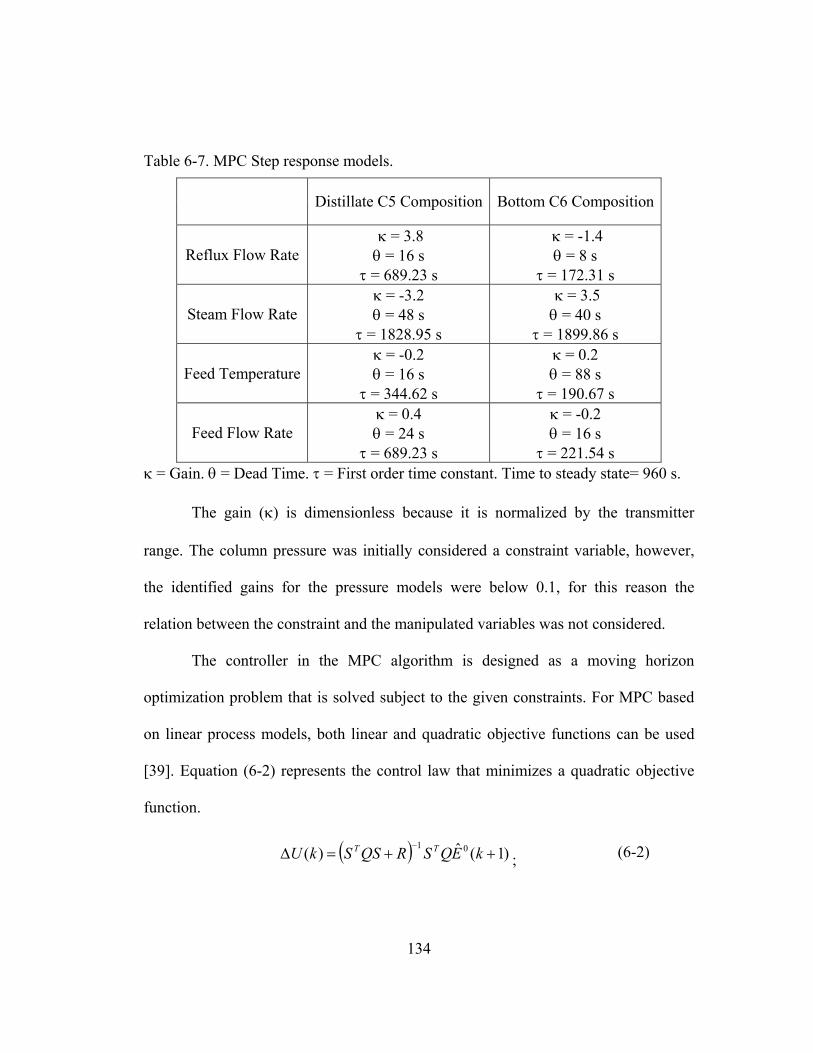
134

Table 6-7. MPC Step response models.

Distillate C5 Composition Bottom C6 Composition

Reflux Flow Rate κ = 3.8 θ = 16 s

τ = 689.23 s

κ = -1.4 θ = 8 s

τ = 172.31 s

Steam Flow Rate κ = -3.2 θ = 48 s

τ = 1828.95 s

κ = 3.5 θ = 40 s

τ = 1899.86 s

Feed Temperature κ = -0.2 θ = 16 s

τ = 344.62 s

κ = 0.2 θ = 88 s

τ = 190.67 s

Feed Flow Rate κ = 0.4 θ = 24 s

τ = 689.23 s

κ = -0.2 θ = 16 s

τ = 221.54 s κ = Gain. θ = Dead Time. τ = First order time constant. Time to steady state= 960 s.

The gain (κ) is dimensionless because it is normalized by the transmitter

range. The column pressure was initially considered a constraint variable, however,

the identified gains for the pressure models were below 0.1, for this reason the

relation between the constraint and the manipulated variables was not considered.

The controller in the MPC algorithm is designed as a moving horizon

optimization problem that is solved subject to the given constraints. For MPC based

on linear process models, both linear and quadratic objective functions can be used

[39]. Equation (6-2) represents the control law that minimizes a quadratic objective

function.

( ) )1(ˆ)( 01++=Δ

− kEQSRQSSkU TT; (6-2)

135

The vector )1(ˆ 0 +kE corresponds to the predicted deviations from the

reference trajectory when no further control action is taken; this vector is known as

the predicted unforced error vector. The matrices Q and R are weighting matrices

used to weight the most important components of the predicted error and control

move, vectors respectively [47]. In DeltaV Predict Pro the elements of Q are known

as penalty on error while the entries of R are the “penalty on move”. The MPC

controller is tuned by modifying the values of the matrices Q and R.

Q allows the output variables to be weighted according to their relative

importance. For implementation R offers convenient tuning parameters because

increasing the values of its elements reduces the magnitude of the input moves

providing a more conservative controller.

Figure 6-10 illustrates the linear MPC performance after a series of step

changes in the distillate and bottoms composition set points. Both output variables

were assigned a penalty on error of one. The penalty on move was set to 25 for the

steam flow rate and 20 for the reflux flow rate. In the experiment the optimizer was

also configured to maximize the concentration of C5 in the distillate. The SP was

allowed to change 0.5% for both controlled variables.

136

58

63

68

73

78

83

88

0 20 40 60 80 100 120 140 160 180 200

Time [min]

Com

posi

tion

[wt%

]

-40

10

60

110

160

210

260

310

360

Flow

Rat

e [lb

/hr]

. Dut

y [B

TU/h

r]

Distillate C5 Composition

Bottom C6 Composition

SP Bottom C6 Composition

SP Distillate C5 Composition

Reboiler Duty

Reflux Flow Rate

SP range = 0.5%

Optimization On Max C5. SP range = 0.5%

Figure 6-10. Composition control using linear MPC.

Given that the system is nonlinear, the tuning parameters in the multivariable

controller were set up to provide robustness and eliminate oscillation in the response.

The main difficulty occurred due to the different gains in the process. The gains

related to the distillate composition were smaller when the azeotropic composition

was reached in the distillate composition than in other regions with lower pentane

recovery in the overhead product. Figure 6-11 illustrates MPC responses inside and

outside the azeotropic region with different tuning parameters. Controller tuning 1 has

a higher penalty on move (PM) for both manipulated variables than controller tuning

2. The parameters used in controller tuning 2 were the values suggested by DeltaV

137

Predict Pro. These values are calculated based on the assumption that the system is

linear. A higher penalty on move improved system stability in the region with higher

gains. The penalty on error was set to 1 for both controlled variables.

68

73

78

83

88

0 20 40 60 80 100 120 140 160

Time [min]

Com

posi

tion

[wt%

]

250

270

290

310

330

350

370

390

Flow

Rat

e [lb

/hr]

. Dut

y [B

TU/h

r]

Distillate C5 Composition Tuning 1 Bottom C6 Composition Tuning 1

SP Bottom C6 Composition SP Distillate C5 Composition

Distillate C5 Composition Tuning 2 Bottom C6 Composition Tuning 2

Feed Flow Rate

Max. C6. SP range = 0.5%

Optimization On Max C5. SP range = 0.5%

PM Tuning 1 Duty=25Reflux=20

PM Tuning 2 Duty=12.5Reflux=9.5

Figure 6-11. MPC behavior using different tuning parameters.

6.2.2.2.1 MPC Response to Measured disturbances

Because instrumentation was available to measure feed temperature and feed

flow rate, these two variables were configured as measured disturbances in the MPC

controller (4X2 configuration). A similar disturbance to the one introduced in the PID

138

controller (see Figure 6-9) was used with the MPC controller under the same

conditions; the results are presented in Figure 6-12.

MPC Control Response to Disturbances in the Feed Temperature

70717273747576777879808182838485868788899091

0 20 40 60 80 100 120

Time (min)

Com

posi

tion

(wt%

)

50

70

90

110

130

150

170

190

Tem

pera

ture

(F)

SP BTT C6

SP BTT C6

Bottom C6

Distillate C5

Feed Temp

Figure 6-12. MPC closed loop response to changes in the feed temperature. PM Tuning: Duty=25, Reflux=20. Data collected from the experiment.

In order to have a fair comparison between the single loop and the

multivariable control strategies, the model predictive control was configured as a 2X2

system without the benefits of disturbance measurements, using reflux flow rate and

steam flow rate as manipulated variables and distillate pentane composition and

bottom’s cyclohexane composition as controlled variables. The MPC responses to

unmeasured disturbances in feed temperature are illustrated in Figure 6-13. The

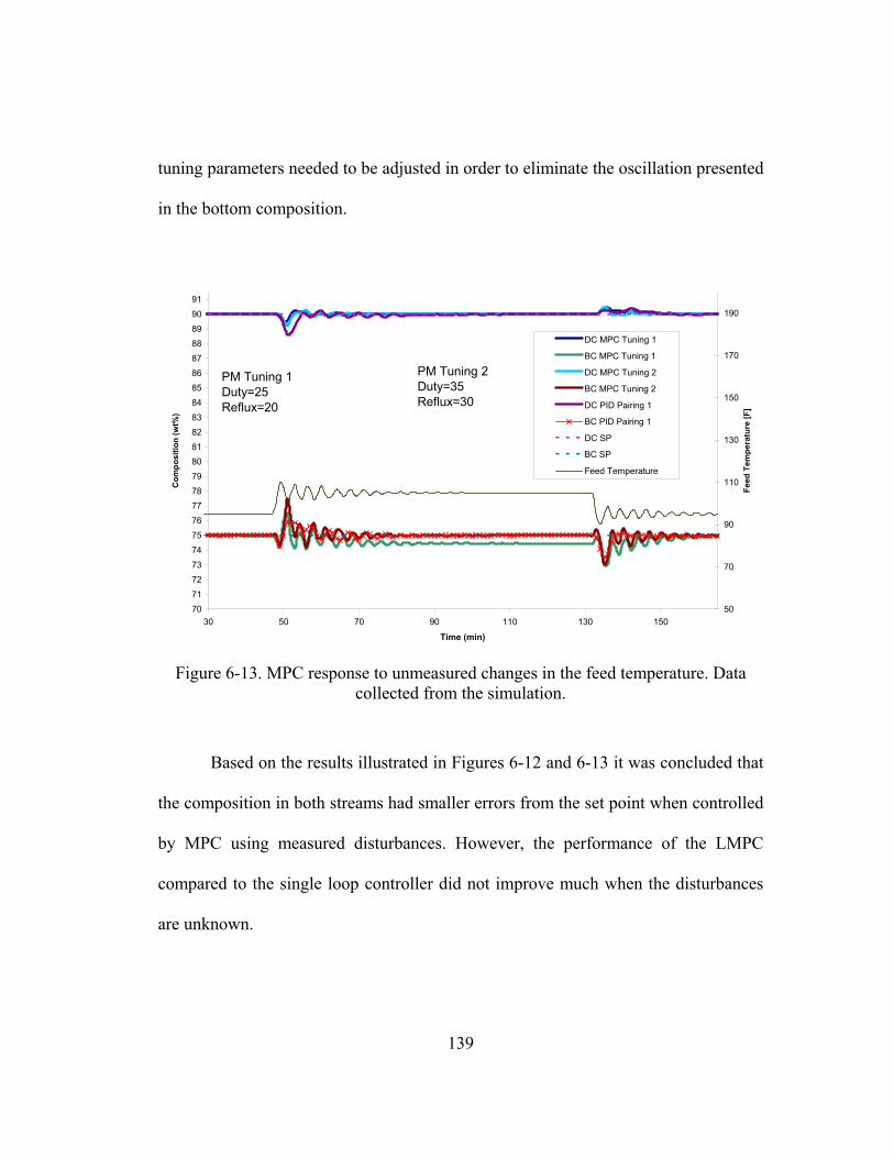
139

tuning parameters needed to be adjusted in order to eliminate the oscillation presented

in the bottom composition.

70717273

74757677787980818283

84858687888990

91

30 50 70 90 110 130 150

Time (min)

Com

posi

tion

(wt%

)

50

70

90

110

130

150

170

190

Feed

Tem

pera

ture

[F]

DC MPC Tuning 1

BC MPC Tuning 1

DC MPC Tuning 2

BC MPC Tuning 2

DC PID Pairing 1

BC PID Pairing 1

DC SP

BC SP

Feed Temperature



Figure 6-13. MPC response to unmeasured changes in the feed temperature. Data

collected from the simulation.

Based on the results illustrated in Figures 6-12 and 6-13 it was concluded that

the composition in both streams had smaller errors from the set point when controlled

by MPC using measured disturbances. However, the performance of the LMPC

compared to the single loop controller did not improve much when the disturbances

are unknown.

140

6.2.2.2.2 MPC Response to Unmeasured disturbances

Besides feed temperature and flow rate, there are other variables that

introduce perturbations to the process such as feed composition, ambient temperature,

steam pressure and temperature, etc. The plant does not have instruments to measure

these variables so they are included in the model predictive control nor are their

values upgraded online in the fundamental dynamic model used in the inferential

control strategy.

The effects of changes in ambient conditions and heating/cooling streams are

reflected in the material distribution in the column which directly affects the

throughput. The online model reconciliation is intended to maintain unaffected the

inferential composition configuration because the model material balance is matched

with the process outputs. For this reason the heat transfer coefficient was one of the

parameters selected for model reconciliation as explained earlier in the chapter.

Figure 6-14 illustrates the controller response under simulation conditions to ambient

temperature unmeasured disturbances. The ambient temperature was increased from

58 F to 77 F, which increased the distillate flow rate from 125lb/hr to 150lb/hr. In

the experiments abrupt changes in the temperature were observed but occurred during

a longer period of time as illustrated in Figure 6-15. The ramp input in the ambient

temperature reflects the actual conditions of the experiment. The controller corrected

very accurately the composition changes due to the temperature disturbances; the

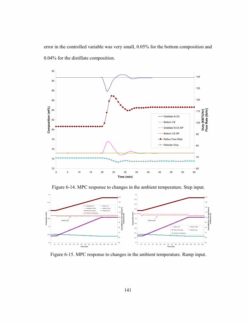
141

error in the controlled variable was very small, 0.05% for the bottom composition and

0.04% for the distillate composition.

72

74

76

78

80

82

84

86

88

90

92

0 5 10 15 20 25 30 35 40 45 50 55 60

Time (min)

Com

posi

tion

(wt%

)

65

75

85

95

105

115

125

135

145

Dut

y [K

BTU

/hr]

Flow

Rat

e [lb

/hr]

Distillate N-C5

Bottom C6

Distillate N-C5 SP

Bottom C6 SP

Reflux Flow Rate

Reboiler Duty

Figure 6-14. MPC response to changes in the ambient temperature. Step input.

89

89.5

90

90.5

91

91.5

92

0 20 40 60 80 100 120 140 160 180 200 220 240 260 280 300 320 340

Time (min)

Com

posi

tion

(wt%

)

55

65

75

85

95

105

115

125

135

145

Dut

y [K

BTU

/hr]

, Flo

w R

ate

[lb/h

r],

Tem

pera

ture

[F]

Distillate N-C5 Bottom C6

Distillate N-C5 SP Bottom C6 SP

Reflux Flow Rate Reboiler Duty

Ambient Temperature

0.04% Error

74

74.2

74.4

74.6

74.8

75

75.2

75.4

75.6

75.8

76

0 20 40 60 80 100 120 140 160 180 200 220 240 260 280 300 320 340

Time (min)

Com

posi

tion

(wt%

)

55

65

75

85

95

105

115

125

135

145

Dut

y [K

BTU

/hr]

, Flo

w R

ate

[lb/h

r],

Tem

pera

ture

[F]

Bottom C6 Bottom C6 SP

Reflux Flow Rate Reboiler Duty

Ambient Temperature

0.05% Error

Figure 6-15. MPC response to changes in the ambient temperature. Ramp input.

142

Changes in the feed composition are more difficult to handle not only because

the challenges imposed in the controller but also because these changes cannot be

upgraded instantaneously in the fundamental dynamic model used to infer

composition. In order to overcome this problem, the feedback loop that introduced the

feed composition disturbance was included in the fundamental model and feed

samples were collected every 20 minutes during the experiments. The controller

response to composition disturbance was studied in a simulation environment; the

results are presented in Figure 6-16. During the test the controller optimizer was set to

maximize the distillate n-pentane and the bottoms cyclohexane composition. This test

introduced larger step changes in the feed composition than the ones observed during

the experiments. The cyclohexane composition did not change more than 5% in the

experiments (see Chapter 5). In the second step change, the methanol composition in

the feed was increased; the controller cannot longer maintain the distillate

composition set point at 90 wt% so it is decreased by the optimizer to 89.5 wt%, in

the same way the set point for the cyclohexane composition in the bottom stream was

decreased from 74.86 wt% to 84.16 wt%.

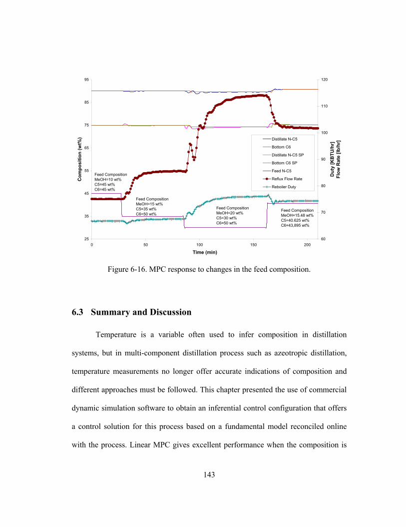
143

25

35

45

55

65

75

85

95

0 50 100 150 200

Time (min)

Com

posi

tion

(wt%

)

60

70

80

90

100

110

120

Dut

y [K

BTU

/hr]

Flow

Rat

e [lb

/hr]

Distillate N-C5

Bottom C6

Distillate N-C5 SP

Bottom C6 SP

Feed N-C5

Reflux Flow Rate

Reboiler Duty

Feed CompositionMeOH=10 wt%C5=45 wt%C6=45 wt%



Feed CompositionMeOH=15.48 wt%C5=40.625 wt%C6=43,895 wt%

Figure 6-16. MPC response to changes in the feed composition.

6.3 Summary and Discussion

Temperature is a variable often used to infer composition in distillation

systems, but in multi-component distillation process such as azeotropic distillation,

temperature measurements no longer offer accurate indications of composition and

different approaches must be followed. This chapter presented the use of commercial

dynamic simulation software to obtain an inferential control configuration that offers

a control solution for this process based on a fundamental model reconciled online

with the process. Linear MPC gives excellent performance when the composition is

144

used directly as a controlled variable and the appropriate tuning is used. A

multivariable controller gave better performance when compared with the traditional

single loop control configuration since there is less interaction between the control

loops.

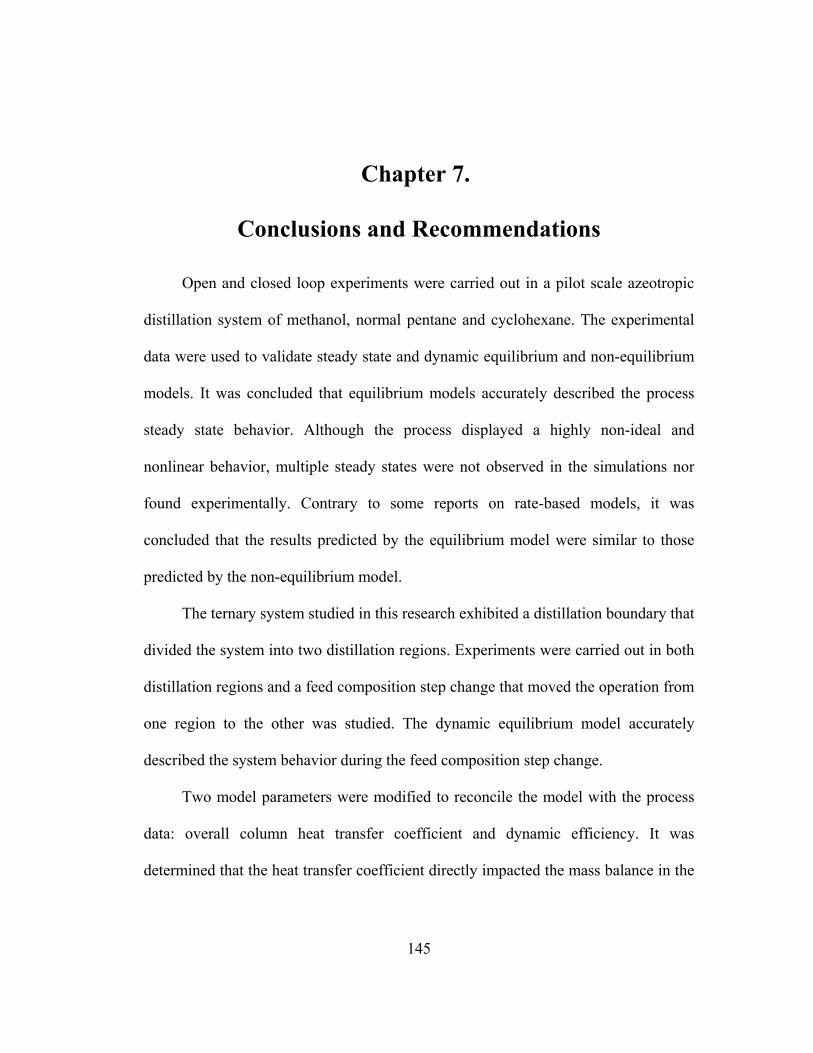
145

Chapter 7.

Conclusions and Recommendations

Open and closed loop experiments were carried out in a pilot scale azeotropic

distillation system of methanol, normal pentane and cyclohexane. The experimental

data were used to validate steady state and dynamic equilibrium and non-equilibrium

models. It was concluded that equilibrium models accurately described the process

steady state behavior. Although the process displayed a highly non-ideal and

nonlinear behavior, multiple steady states were not observed in the simulations nor

found experimentally. Contrary to some reports on rate-based models, it was

concluded that the results predicted by the equilibrium model were similar to those

predicted by the non-equilibrium model.

The ternary system studied in this research exhibited a distillation boundary that

divided the system into two distillation regions. Experiments were carried out in both

distillation regions and a feed composition step change that moved the operation from

one region to the other was studied. The dynamic equilibrium model accurately

described the system behavior during the feed composition step change.

Two model parameters were modified to reconcile the model with the process

data: overall column heat transfer coefficient and dynamic efficiency. It was

determined that the heat transfer coefficient directly impacted the mass balance in the

146

system since it modified the heat loss in the column. For these reason it was used to

reconcile the distillate flow rate in the model with process output. The dynamic

efficiency parameter used in HYSYS is defined differently from the Murphree

efficiency used in the steady state models and was used to account for the non-

equilibrium generated by the dynamic changes in the column. These two parameters

were found to have fairly similar values in the two distillation regions.

The dynamic model was used to obtain an inferential control solution based on

an online model reconciliation configuration that matched the model predictions with

the process outputs. Temperature has been the variable of choice when controlling

composition in a distillation column, but in multicomponent distillation temperature

measurements do not offer accurate indications of composition, hence commercial

dynamic simulation software was used to obtain an inferential control solution.

Multivariable control strategies were studied by analyzing the performance of

PID controllers using two different variable pairings and model-based control. Linear

MPC based on Emerson Process Management PredictPro achieved improves

performance when the composition was used directly as a controlled variable with the

appropriate tuning.

7.1 Contributions

The major contributions of this research are summarized below:

147

1. A large pilot-scale distillation column was configured with instrumentation and

automated control system to run multicomponent distillation experiments.

2. Dynamic and steady-state multicomponent distillation experiments were carried

out and experimental process data were collected using a pilot scale experimental

set-up. Available published distillation data predominantly comes from

experiments on lab scale equipment.

3. Equilibrium and non-equilibrium steady state models for azeotropic distillation

were developed and validated.

4. In comparing equilibrium and non-equilibrium models performance, it was

demonstrated that the results predicted by the equilibrium model were similar to

those of the non-equilibrium model. Equilibrium models accurately describe

azeotropic behavior and more research needs to be done in developing good mass

and heat transfer coefficient models for non-equilibrium models.

5. Fundamental dynamic model was validated based on dynamic testing of an

azeotropic distillation column.

6. An online model reconciliation module was designed and validated for dynamic

distillation models.

7. A new approach of inferential control of composition was proposed and validated

experimentally.

8. Different control approaches were studied and compared for the azeotropic

distillation process including different variable pairing with PID controllers.

148

9. Linear model predictive control with appropriate tuning provided excellent

experimental control of multicomponent distillation when the composition is used

directly as a controlled variable.

7.2 Future Work

The experimental system used in this research was a highly non-ideal

multicomponent system whose results could be applied to azeotropic distillation.

Published experimental data on industrial applications of azeotropic distillation is

scarce. By performing some modifications to the pilot plant an industrial application

using an entrainer and including phase separation using the accumulator as decanter

could be studied in the system.

The experimental set-up was originally designed as a reactive distillation

system and models developed for this system are still pending to be validated. During

this research it was determined that the recycle loop needs to be eliminated in order

for the reactive distillation experiments to be successful. The tools and configuration

developed in this research could be used in the validation of such models.

149

Appendix A. Analytical Procedure for Methanol, Normal Pentane

and Cyclohexane

An analytical procedure for the analysis of the samples collected from the

system was developed and implemented in two HP 5890 gas chromatographs. The

basic setup and calibration as well as the procedure to analyze the samples are

described in the following sections.

A.1 Basic Chromatograph Set Up The HP 5890 gas chromatographs used for the composition analysis operated

with a capillary column and a flame ion detector (FID). This type of detector only

identifies carbon molecules; it gives a voltage proportional to the flow of ions that are

formed when carbon molecules are combusted.

The analysis was developed using ultra high purity helium as the carrier gas,

and ultra high purity hydrogen and zero grade air for the combustion. The gas

chromatograph elements and operating conditions are listed in Table A- 1.

150

Table A- 1 Gas Chromatograph Conditions

GC column :

BP-PONA, 20m long, 0.15mm diameter,

film thickness: 0.25um

BP-PONA, 8m long, 0.15mm diameter,

film thickness: 0.25um

Carrier Gas Helium Flow: 0.75ml/min Cylinder regulator pressure: 40 psig

FID Gases Hydrogen Flow: 30ml/min Cylinder regulator pressure: 15 psig

Air Flow: 350ml/min Cylinder regulator pressure: 40 psig

Injector Split ratio 100:1 Septa purge 75ml/min

Detector Flame ion detector Column Pressure

#1 22 psig #2 5 psig

The readings from the instruments were collected digitally using the

EZChrom Elite data system from SCIENTIFIC Software. The gas chromatographs

were interfaced to a computer (EZserver) through a SS420X module designed to

collect the analog data from the instrument and to send it to the controlling computer

via a standard RS-232C serial interface.

The application in the computer was divided into two areas. One used to

access to the chromatographs real time data and the other used for offline processing.

151

One method was developed for each gas chromatograph using the response calculated

with linear curve fitting, and used for every data file acquired in the respective

instrument. The data files could be processed offline using different methods if desire.

A.2 Oven Program Six quantities must be introduced to the gas chromatograph in order to

configure the oven program: initial temperature, initial time, rate, final temperature,

final time, and injector temperature. The following procedure describes the oven

algorithm when a sample is analyzed:

1) Oven is at the initial temperature value. The sample is injected for the

analytical procedure to start.

2) The oven maintains the initial temperature for the amount of time given by

the initial time value.

3) The temperature in the oven is increased at the rate value; this value is given

in units of temperature per time unit (i.e. °C/min).

4) The oven temperature reaches the final temperature value.

5) The oven holds the final temperature value for a time interval given by the

final time value and the detection is terminated.

Secondary temperature ramps can be also configured to start and stop at specific

temperatures. The injector temperature should be set very high to ensure all the

components vaporize. The detector’s maximum temperature for the HP 5890 gas

chromatographs is 320°C. The oven program is summarized in Table A- 2.

152

Table A- 2. Oven Program

Initial Temperature 40oC

Initial Time 2 min

Rate 10 oC/min

Final Temperature 100 oC

Final Time 2 min

Detector Temperature FID set at 320oC

A.3 Calibration The procedure followed in the calibration of the instruments consisted in

standard preparation, sample detection, and linear calibration curve elaboration to

determine response factors. Every different component had its own response factor

that was calculated to give the component weigh percent after multiplied by the area

count collected from the gas chromatograph.

A.3.1 Preparation of Samples Since it was necessary to have single phase samples a solvent was used to

make homogeneous one phase solutions. The solvent was selected to ensure no

chemical reaction in the solution that would modify the original amount of materials

in the mixture. The samples were made based on weight percent because the

composition analysis needed was weight based.

153

Standards representing the total concentration range under evaluation were

developed by weighing out the components added to a vial on a high fidelity

laboratory scale. Vials were sealed with a septum and used within short periods of

time.

A.3.2 Shooting the Samples The injection size used was 1 micro liter. A syringe with a repeating adapter

was used to ensure repeatability. The following injection procedure was followed:

1) Insert the needle into the sample and pump the plunger a few times. Pumping

the plunger ensures no vapor is left in the syringe.

2) Insert the needle into the chromatograph’s injector and immediately inject the

sample and press start.

3) Leave the needle in the injection port for about two or three seconds after the

plunger has been pushed.

A.3.3 Determining the Response Factors

In order to determine the response factors the retention time of each

component was first identified by shutting samples containing only one pure

component into each gas chromatograph. This operation also provided the individual

components peak forms. After the retention times and peaks were determined three

test samples were analyzed five times each to obtain the instrument precision in the

area count measurement. It was concluded that the repeatability of the sample was

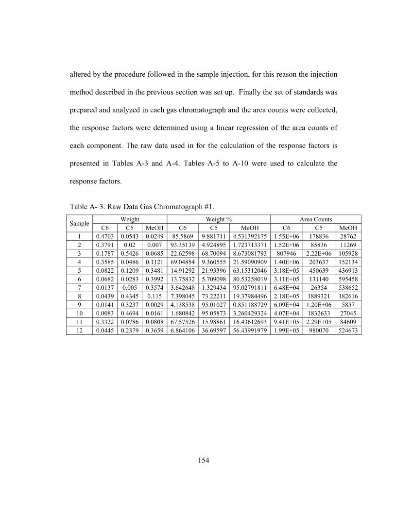
154

altered by the procedure followed in the sample injection, for this reason the injection

method described in the previous section was set up. Finally the set of standards was

prepared and analyzed in each gas chromatograph and the area counts were collected,

the response factors were determined using a linear regression of the area counts of

each component. The raw data used in for the calculation of the response factors is

presented in Tables A-3 and A-4. Tables A-5 to A-10 were used to calculate the

response factors.

Table A- 3. Raw Data Gas Chromatograph #1. Weight Weight % Area Counts Sample

C6 C5 MeOH C6 C5 MeOH C6 C5 MeOH 1 0.4703 0.0543 0.0249 85.5869 9.881711 4.531392175 1.55E+06 178836 28762 2 0.3791 0.02 0.007 93.35139 4.924895 1.723713371 1.52E+06 85836 11269 3 0.1787 0.5426 0.0685 22.62598 68.70094 8.673081793 807946 2.22E+06 105928 4 0.3585 0.0486 0.1121 69.04854 9.360555 21.59090909 1.40E+06 203637 152134 5 0.0822 0.1209 0.3481 14.91292 21.93396 63.15312046 3.18E+05 450639 436913 6 0.0682 0.0283 0.3992 13.75832 5.709098 80.53258019 3.11E+05 131140 595458 7 0.0137 0.005 0.3574 3.642648 1.329434 95.02791811 6.48E+04 26354 538652 8 0.0439 0.4345 0.115 7.398045 73.22211 19.37984496 2.18E+05 1889321 182616 9 0.0141 0.3237 0.0029 4.138538 95.01027 0.851188729 6.09E+04 1.20E+06 5857

10 0.0083 0.4694 0.0161 1.680842 95.05873 3.260429324 4.07E+04 1832633 27045 11 0.3322 0.0786 0.0808 67.57526 15.98861 16.43612693 9.41E+05 2.29E+05 84609 12 0.0445 0.2379 0.3659 6.864106 36.69597 56.43991979 1.99E+05 980070 524673

155

Table A- 4. Raw Data Gas Chromatograph #2. Weight Weight % Area Counts

Sample C6 C5 MeOH C6 C5 MeOH C6 C5 MeOH

1 0.4703 0.0543 0.0249 85.5869 9.881711 4.531392175 6.51E+05 75038 11549 2 0.3791 0.02 0.007 93.35139 4.924895 1.723713371 5.80E+05 32338 4216 3 0.1787 0.5426 0.0685 22.62598 68.70094 8.673081793 335640 9.41E+05 40729 4 0.3585 0.0486 0.1121 69.04854 9.360555 21.59090909 5.87E+05 85615 59509 5 0.0822 0.1209 0.3481 14.91292 21.93396 63.15312046 1.36E+05 192803 176658 6 0.0682 0.0283 0.3992 13.75832 5.709098 80.53258019 1.31E+05 55495 237504 7 0.0137 0.005 0.3574 3.642648 1.329434 95.02791811 2.49E+04 10022 190323 8 0.0439 0.4345 0.115 7.398045 73.22211 19.37984496 9.32E+04 809645 72272 9 0.0141 0.3237 0.0029 4.138538 95.01027 0.851188729 2.77E+04 5.44E+05 2401

10 0.0083 0.4694 0.0161 1.680842 95.05873 3.260429324 1.39E+04 754053 9924 11 0.3322 0.0786 0.0808 67.57526 15.98861 16.43612693 4.23E+05 1.03E+05 34607 12 0.0445 0.2379 0.3659 6.864106 36.69597 56.43991979 7.63E+04 377120 189915

Table A- 5. Linear Regression Analysis for Cyclohexane. GC #1.

Sample Actual wt. Actual area Calculated wt. 1 0.4703 1.55E+06 0.4323 2 0.3791 1.52E+06 0.4258 3 0.1787 8.08E+05 0.2256 4 0.3585 1.40E+06 0.3911 5 0.0822 3.18E+05 0.0889 6 0.0682 3.11E+05 0.0869 7 0.0137 6.48E+04 0.0181 8 0.0439 2.18E+05 0.0610 9 0.0141 6.09E+04 0.0170

10 0.0083 4.07E+04 0.0114 11 0.3322 9.41E+05 0.2627 12 0.0445 1.99E+05 0.0555

Linear Regression analysis (line slop) 3581723.1729

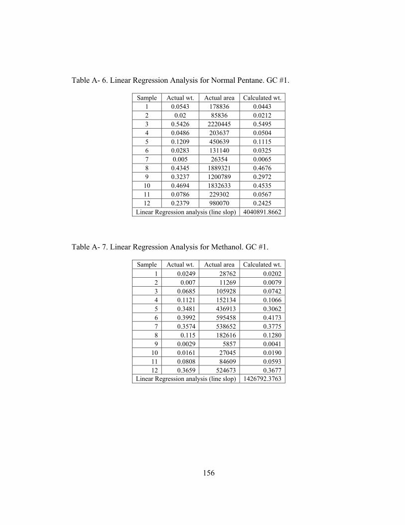
156

Table A- 6. Linear Regression Analysis for Normal Pentane. GC #1.

Sample Actual wt. Actual area Calculated wt. 1 0.0543 178836 0.0443 2 0.02 85836 0.0212 3 0.5426 2220445 0.5495 4 0.0486 203637 0.0504 5 0.1209 450639 0.1115 6 0.0283 131140 0.0325 7 0.005 26354 0.0065 8 0.4345 1889321 0.4676 9 0.3237 1200789 0.2972

10 0.4694 1832633 0.4535 11 0.0786 229302 0.0567 12 0.2379 980070 0.2425


Table A- 7. Linear Regression Analysis for Methanol. GC #1.


10 0.0161 27045 0.0190 11 0.0808 84609 0.0593 12 0.3659 524673 0.3677


157

Table A- 8. Linear Regression Analysis for Cyclohexane. GC #2.

Sample Actual wt. Actual area Calculated wt. 1 0.4703 6.51E+05 0.4392 2 0.3791 5.80E+05 0.3913 3 0.1787 3.36E+05 0.2264 4 0.3585 5.87E+05 0.3962 5 0.0822 1.36E+05 0.0918 6 0.0682 1.31E+05 0.0886 7 0.0137 2.49E+04 0.0168 8 0.0439 9.32E+04 0.0628 9 0.0141 2.77E+04 0.0187

10 0.0083 1.39E+04 0.0094 11 0.3322 4.23E+05 0.2856 12 0.0445 7.63E+04 0.0515


Table A- 9. Linear Regression Analysis for Pentane. GC #2.


10 0.4694 754053 0.4416 11 0.0786 102878 0.0602 12 0.2379 377120 0.2208


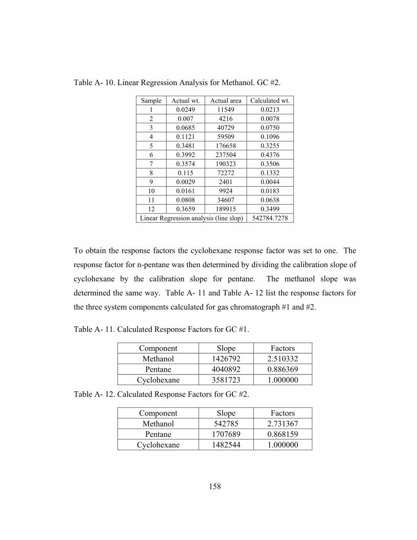
158

Table A- 10. Linear Regression Analysis for Methanol. GC #2.


10 0.0161 9924 0.0183 11 0.0808 34607 0.0638 12 0.3659 189915 0.3499


To obtain the response factors the cyclohexane response factor was set to one. The

response factor for n-pentane was then determined by dividing the calibration slope of

cyclohexane by the calibration slope for pentane. The methanol slope was

determined the same way. Table A- 11 and Table A- 12 list the response factors for

the three system components calculated for gas chromatograph #1 and #2.

Table A- 11. Calculated Response Factors for GC #1.

Component Slope Factors Methanol 1426792 2.510332 Pentane 4040892 0.886369

Cyclohexane 3581723 1.000000

Table A- 12. Calculated Response Factors for GC #2.

Component Slope Factors Methanol 542785 2.731367 Pentane 1707689 0.868159

Cyclohexane 1482544 1.000000

159

The calculated and actual data were compared with another linear regression to

validate the analytical procedure.

Methanol

y = 1.0266xR2 = 0.9994

0

20

40

60

80

100

120

0 10 20 30 40 50 60 70 80 90 100

Calculated wt%

Act

ual w

t%

wt% MethanolLinear (wt% Methanol)

Figure A- 1. Linear Regression Actual vs. Calculated Methanol Concentration in GC #1.

160

Pentane

y = 1.0245xR2 = 0.9994

0

20

40

60

80

100

120

0 10 20 30 40 50 60 70 80 90 100

Calculated wt%

Act

ual w

t%

wt% PentaneLinear (wt% Pentane)

Figure A- 2. Linear Regression Actual vs. Calculated Pentane Concentration in GC #1.

Cyclohexane

y = 0.9759xR2 = 0.9977

0

10

20

30

40

50

60

70

80

90

100

0 10 20 30 40 50 60 70 80 90 100

Calculated wt%

Act

ual w

t%

wt% CyclohexaneLinear (wt% Cyclohexane)

Figure A- 3. Linear Regression Actual vs. Calculated Cyclohexane Concentration in GC #1.

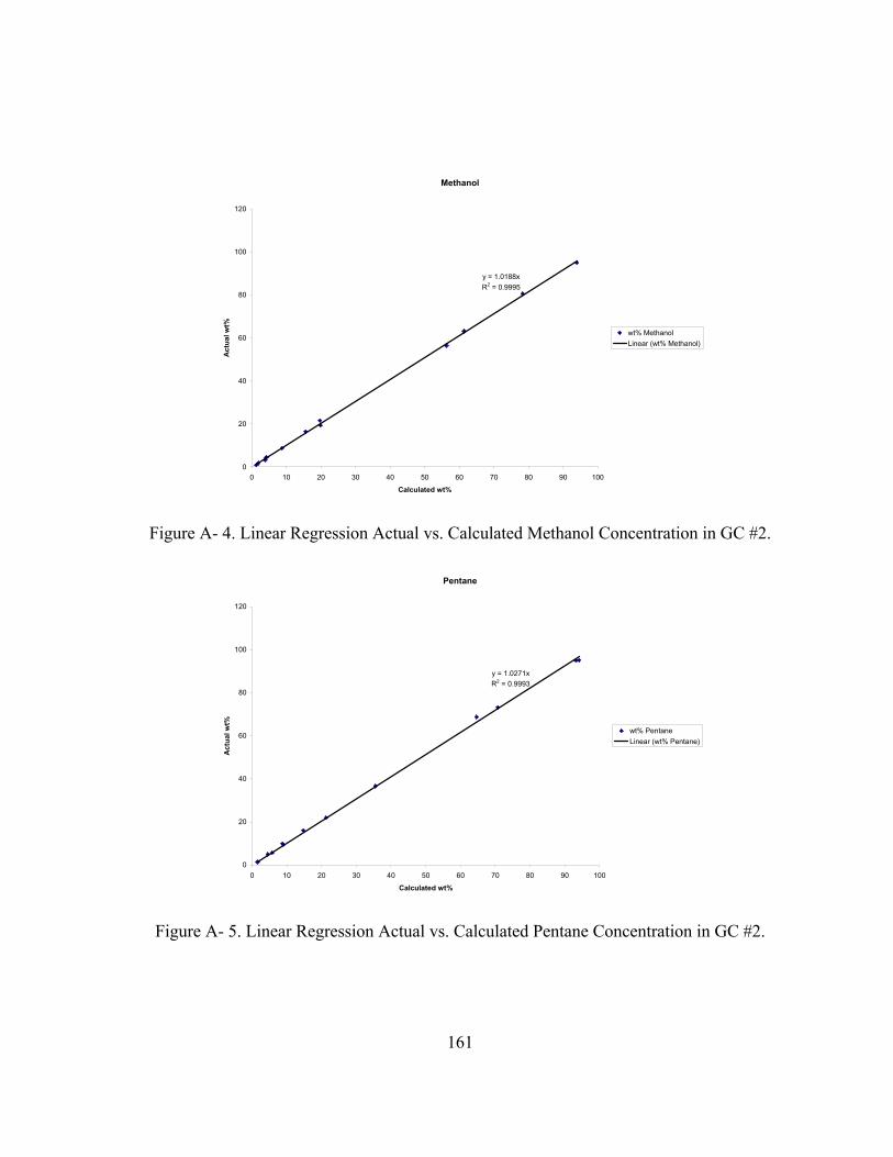
161

Methanol

y = 1.0188xR2 = 0.9995

0

20

40

60

80

100

120

0 10 20 30 40 50 60 70 80 90 100

Calculated wt%

Act

ual w

t%

wt% MethanolLinear (wt% Methanol)

Figure A- 4. Linear Regression Actual vs. Calculated Methanol Concentration in GC #2.

Pentane

y = 1.0271xR2 = 0.9993

0

20

40

60

80

100

120

0 10 20 30 40 50 60 70 80 90 100

Calculated wt%

Act

ual w

t%

wt% PentaneLinear (wt% Pentane)


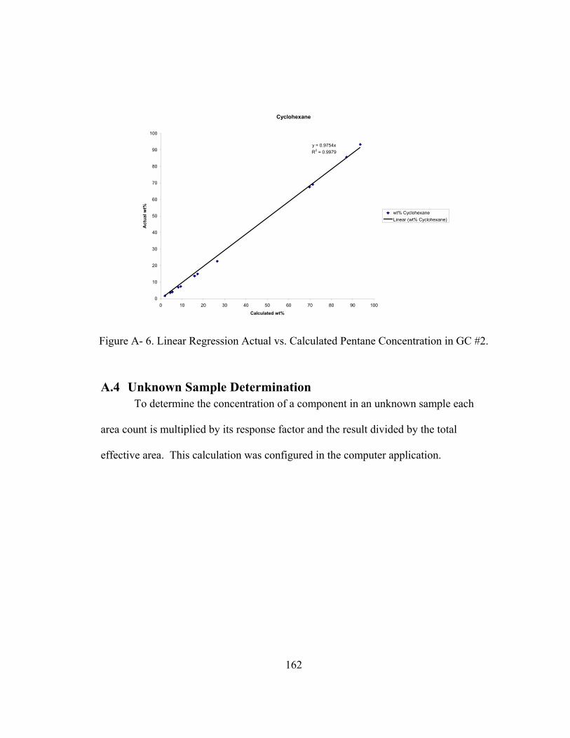
162

Cyclohexane

y = 0.9754xR2 = 0.9979

0

10

20

30

40

50

60

70

80

90

100

0 10 20 30 40 50 60 70 80 90 100

Calculated wt%

Act

ual w

t%

wt% CyclohexaneLinear (wt% Cyclohexane)


A.4 Unknown Sample Determination To determine the concentration of a component in an unknown sample each

area count is multiplied by its response factor and the result divided by the total

effective area. This calculation was configured in the computer application.

163

Appendix B. Data from Experiments and Models

B.1 Steady State Experimental Data

Table B- 1. Steady State First Distillation region.

# Overhead

Vapor Temp.

Stage 6 Temp.

Stage 8 Temp.

Stage 9 Tempe.

Stage 11 Temp.

Stage 13 Temp.

Stage 15 Temp.

Stage 16 Temp.

Stage 21 Temp.

Stage 22 Temp.

TT621 TT6079 TT6078 TT6077 TT6076 TT6075 TT6074 TT6073 TT6072 TT6071 (F) (F) (F) (F) (F) (F) (F) (F) (F) (F) 1 105.56 107.61 107.78 108.73 108.66 110.04 112.97 115.14 132.55 147.14 2 105.93 107.91 108.21 109.24 109.42 111.00 114.07 115.91 132.80 149.99 3 104.00 108.80 108.84 109.57 109.07 109.42 110.20 110.96 132.31 140.84 4 104.44 107.87 108.11 108.70 108.32 108.82 109.71 110.65 132.38 142.25 5 103.58 108.73 109.30 110.10 109.69 109.94 110.51 110.93 131.84 138.98 6 107.40 111.04 111.20 111.83 111.28 111.58 112.02 112.22 130.04 145.21 7 107.49 111.77 111.92 112.44 111.96 112.23 112.64 112.68 129.94 144.11 8 106.26 108.21 108.33 109.25 109.19 110.48 113.45 115.59 132.65 147.55

# Boil up Temp.

Column Bottom's Temp.

Feed Temp.

Overhead Liquid Temp.

Cold Water In

Cold Water Out

Steam Temp.

Steam Cond. Temp.

Level Column's Bottom

Level Reboiler

TT605 TT604 TT610 TT625 TT624 TT626 TT602 TT603 LT601 LT602 (F) (F) (F) (F) (F) (F) (F) (F) (in) (in) 1 172.96 165.87 94.79 90.16 62.13 76.11 326.18 179.90 15.00 11.80 2 175.24 173.47 94.79 95.33 63.70 78.41 325.99 182.77 15.23 11.56 3 162.06 158.43 95.25 89.70 63.78 77.02 326.85 169.45 14.67 11.65 4 164.56 160.00 95.60 86.42 63.15 76.16 334.03 171.89 14.67 11.74 5 158.64 157.91 90.28 73.86 52.87 66.16 343.58 168.89 15.45 11.78 6 173.03 171.41 89.55 74.68 53.36 66.95 343.41 168.55 15.12 11.94 7 171.39 169.43 89.89 79.40 54.71 69.98 338.15 177.86 15.49 11.69 8 172.48 171.28 94.98 79.02 56.19 70.16 337.88 180.23 14.83 11.17

# Reboiler Duty

Steam Pressure

Column Pressure

Column Pressure

Drop

Feed Flow Rate

Bottom Flow Rate

Steam Flow Rate

Reflux Flow Rate


Cold Water Flow Rate

QIC602 PT202 PT615 PDT610 FT600 FT601 FT602 FT603 FT604 FT605 (MMBTU/hr) (psia) (psi) (inH20) (PPH) (PPH) (PPH) (PPH) (PPH) (PPH) 1 69.04 106.05 6.00 2.97 299.96 156.03 67.26 74.87 144.05 4.86 2 77.42 106.22 5.97 3.36 299.74 139.42 75.14 75.41 160.62 4.86 3 68.84 107.05 5.97 2.74 300.02 201.28 65.21 100.14 99.13 4.86 4 68.50 116.15 5.99 2.80 299.30 191.97 64.75 90.82 107.65 4.86 5 69.33 129.97 6.00 2.80 300.12 220.35 65.07 109.74 79.32 4.86 6 69.00 129.79 5.98 2.69 200.39 100.00 65.18 120.64 100.00 4.86 7 75.49 121.77 5.88 4.01 200.60 111.88 71.75 149.90 88.46 4.86 8 69.78 120.79 5.97 2.88 300.83 148.70 66.76 75.56 151.42 4.86 # Feed Feed Feed Distillate Distillate Distillate Bottom Bottom Bottom Level Acc.

Weight Percent

Weight Percent

Weight Percent

Weight Percent

Weight Percent

Weight Percent

Weight Percent

Weight Percent

Weight Percent LT603

MeOH C5 C6 MeOH C5 C6 MeOH C5 C6 (in) 1 4.06 49.34 46.60 6.74 93.08 0.18 0.13 15.37 84.50 13.08 2 3.96 51.52 44.52 6.85 92.96 0.19 0.16 12.47 87.37 13.05 3 3.27 43.65 53.09 8.92 90.83 0.25 0.13 22.03 77.84 13.45 4 3.67 44.15 52.18 8.66 91.29 0.06 0.00 20.70 79.30 13.01 5 2.95 41.77 55.29 8.75 90.92 0.33 0.05 24.35 75.60 12.79 6 3.28 51.10 45.62 4.34 95.26 0.40 0.08 13.34 86.57 12.27 7 3.02 48.06 48.92 6.33 93.64 0.03 0.00 15.06 84.94 12.97 8 4.06 52.11 43.83 5.99 93.84 0.17 0.06 11.13 88.81 13.12

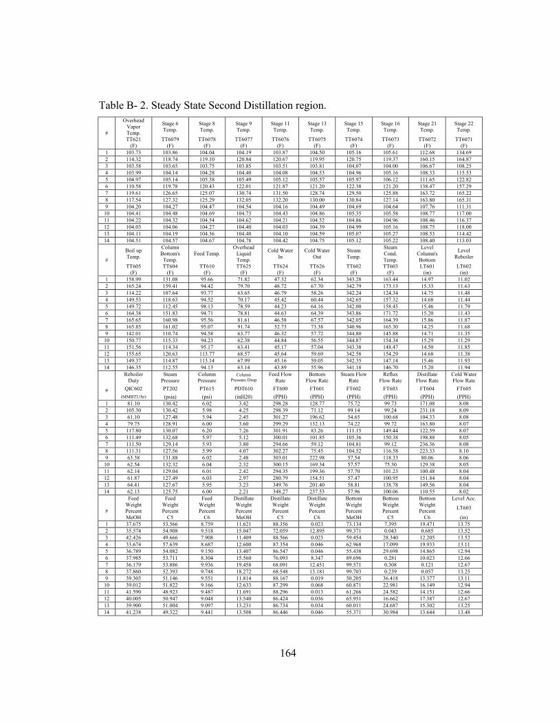
164

Table B- 2. Steady State Second Distillation region.

#

Overhead Vapor Temp.

Stage 6 Temp.

Stage 8 Temp.

Stage 9 Temp.

Stage 11 Temp.

Stage 13 Temp.

Stage 15 Temp.

Stage 16 Temp.

Stage 21 Temp.

Stage 22 Temp.

TT621 TT6079 TT6078 TT6077 TT6076 TT6075 TT6074 TT6073 TT6072 TT6071 (F) (F) (F) (F) (F) (F) (F) (F) (F) (F) 1 103.73 103.86 104.04 104.19 103.87 104.50 105.16 105.61 112.68 134.69 2 114.32 118.74 119.10 120.84 120.67 119.95 120.75 119.37 160.15 164.87 3 103.58 103.65 103.75 103.85 103.51 103.81 104.07 104.00 106.67 108.25 4 103.99 104.14 104.28 104.40 104.08 104.53 104.96 105.16 108.33 115.53 5 104.97 105.14 105.38 105.49 105.12 105.57 105.97 106.12 111.65 122.82 6 110.58 119.78 120.43 122.01 121.87 121.20 122.38 121.20 138.47 157.29 7 119.61 126.65 125.07 130.74 131.50 128.74 129.50 125.88 163.72 165.22 8 117.54 127.32 125.29 132.05 132.20 130.00 130.84 127.14 163.80 165.31 9 104.20 104.27 104.47 104.54 104.16 104.49 104.69 104.64 107.76 111.31 10 104.41 104.48 104.69 104.73 104.43 104.86 105.35 105.58 108.77 117.00 11 104.22 104.32 104.54 104.62 104.21 104.52 104.86 104.96 108.46 116.37 12 104.03 104.06 104.27 104.40 104.03 104.39 104.99 105.16 108.75 118.00 13 104.11 104.19 104.36 104.40 104.10 104.59 105.07 105.27 108.53 114.42 14 104.51 104.57 104.67 104.78 104.42 104.75 105.12 105.22 108.40 113.03

#

Boil up Temp.


Feed Temp. Overhead

Liquid Temp.

Cold Water In

Cold Water Out

Steam Temp.

Steam Cond. Temp.


Level Reboiler

TT605 TT604 TT610 TT625 TT624 TT626 TT602 TT603 LT601 LT602 (F) (F) (F) (F) (F) (F) (F) (F) (in) (in) 1 158.99 131.08 95.66 71.82 47.32 62.34 343.28 163.44 14.97 11.02 2 165.24 159.41 94.42 79.70 48.72 67.70 342.79 173.13 15.33 11.63 3 114.22 107.64 93.77 63.65 46.79 58.26 342.24 124.34 14.75 11.48 4 149.53 118.63 94.52 70.17 45.42 60.44 342.65 157.32 14.68 11.44 5 149.72 112.45 98.13 78.59 44.23 64.16 342.00 158.45 15.46 11.79 6 164.38 151.83 94.71 78.81 44.63 64.39 343.86 171.72 15.20 11.43 7 165.65 160.98 95.56 81.61 46.58 67.57 342.05 164.39 15.86 11.87 8 165.85 161.02 95.07 91.74 52.73 73.38 340.96 165.30 14.25 11.68 9 142.01 110.74 94.58 63.77 46.32 57.72 344.80 145.88 14.71 11.35 10 150.77 115.33 94.23 62.38 44.84 56.55 344.87 154.34 15.29 11.29 11 151.56 114.34 95.17 63.41 45.17 57.04 343.38 148.47 14.50 11.85 12 155.65 120.63 113.77 68.57 45.64 59.69 342.58 154.29 14.68 11.38 13 149.37 114.87 113.14 67.99 45.16 59.05 342.35 147.14 15.46 11.93 14 146.35 112.55 94.13 63.14 43.89 55.96 341.18 146.70 15.20 11.94

Reboiler

Duty Steam

Pressure Column Pressure

Column Pressure Drop

Feed Flow Rate

Bottom Flow Rate

Steam Flow Rate

Reflux Flow Rate



# QIC602 PT202 PT615 PDT610 FT600 FT601 FT602 FT603 FT604 FT605 (MMBTU/hr) (psia) (psi) (inH20) (PPH) (PPH) (PPH) (PPH) (PPH) (PPH) 1 81.10 130.42 6.02 3.42 298.28 128.77 75.72 99.73 171.08 8.08 2 105.30 130.42 5.98 4.25 298.39 71.12 99.14 99.24 231.18 8.09 3 61.10 127.48 5.94 2.45 301.27 196.62 54.65 100.68 104.33 8.08 4 79.75 128.91 6.00 3.60 299.29 132.13 74.22 99.72 163.80 8.07 5 117.80 130.07 6.20 7.26 301.91 83.26 111.15 149.44 122.59 8.07 6 111.49 132.68 5.97 5.12 300.01 101.85 105.36 150.38 198.88 8.05 7 111.50 129.14 5.93 3.80 294.66 59.12 104.81 99.12 236.36 8.08 8 111.31 127.56 5.99 4.07 302.27 75.45 104.52 116.58 223.33 8.10 9 63.38 131.88 6.02 2.48 303.01 222.98 57.54 118.33 80.06 8.06 10 62.54 132.32 6.04 2.32 300.15 169.34 57.57 75.30 129.38 8.05 11 62.14 129.04 6.01 2.42 294.35 199.36 57.70 101.23 100.48 8.04 12 61.87 127.49 6.03 2.97 280.79 154.51 57.47 100.95 151.84 8.04 13 64.41 127.67 5.95 3.23 349.76 201.40 58.81 138.78 149.56 8.04 14 62.13 125.75 6.00 2.21 348.27 237.53 57.96 100.06 110.55 8.02 Feed Feed Feed Distillate Distillate Distillate Bottom Bottom Bottom Level Acc.

# Weight Percent

Weight Percent

Weight Percent

Weight Percent

Weight Percent

Weight Percent

Weight Percent

Weight Percent

Weight Percent LT603

MeOH C5 C6 MeOH C5 C6 MeOH C5 C6 (in) 1 37.675 53.566 8.759 11.621 88.356 0.023 73.134 7.395 19.471 13.75 2 35.574 54.908 9.518 15.047 72.059 12.895 99.371 0.043 0.685 13.52 3 42.426 49.666 7.908 11.409 88.566 0.023 59.454 28.340 12.205 13.52 4 33.674 57.639 8.687 12.600 87.354 0.046 62.968 17.099 19.933 13.11 5 36.789 54.082 9.150 13.407 86.547 0.046 55.438 29.698 14.865 12.94 6 37.985 53.711 8.304 15.560 76.093 8.347 89.696 0.281 10.023 12.66 7 36.179 53.886 9.936 19.458 68.091 12.451 99.571 0.308 0.121 12.67 8 37.860 52.393 9.748 18.272 68.548 13.181 99.703 0.239 0.057 13.25 9 39.303 51.146 9.551 11.814 88.167 0.019 50.205 36.418 13.377 13.11 10 39.012 51.822 9.166 12.633 87.299 0.068 60.871 22.981 16.149 12.94 11 41.590 48.923 9.487 11.691 88.296 0.013 61.266 24.582 14.151 12.66 12 40.005 50.947 9.048 13.540 86.424 0.036 65.951 16.662 17.387 12.67 13 39.900 51.004 9.097 13.231 86.734 0.034 60.011 24.687 15.302 13.25 14 41.238 49.322 9.441 13.508 86.446 0.046 55.371 30.984 13.644 13.48

165

B.2 Steady State Simulated Data Table B-3. Composition data [wt%] from Aspen Plus equilibrium model. First distillation region.

# Distillate Bottom MeOH C5 C6 MeOH C5 C6 1 8.458 91.537 0.005 0.000 10.389 89.611 2 7.397 92.566 0.037 0.000 4.232 95.768 3 9.908 90.092 0.000 0.000 20.769 79.231 4 10.194 89.806 0.000 0.000 18.469 81.531 5 11.061 88.939 0.000 0.000 24.612 75.388 6 6.560 93.440 0.000 0.000 8.760 91.240 7 6.864 93.136 0.000 0.000 12.643 87.357 8 8.050 91.943 0.007 0.000 11.581 88.419

Average Error % -1.489 1.296 0.194 1.143 -0.994 -0.150 Error Standard Deviation 0.720 0.650 0.125 0.721 0.646 0.115

Table B-4. Composition data [Wt%] from Aspen Plus rate-based model. First distillation region. (26 segments – Onda et al. model)


Average Error % -1.741 2.528 -0.787 1.143 -3.353 2.209 Error Standard Deviation 0.588 1.412 1.316 0.721 3.991 4.054

Table B-5. Composition data [Wt%] from Aspen Plus rate-based model. First distillation region. (52 segments – Onda et al. model)



Table B- 6. Composition Data [Wt%] from Aspen Plus Rate-based Model. First Distillation Region. (52 segments – Billet & Schultes model)



166

B-7. Composition data [Wt%] from Aspen Plus non-equilibrium model. First distillation region. Onda et al. correlation. No interfacial heat transfer.



Table B-8. Composition data [Wt%] from Aspen Plus non-equilibrium model. First distillation region. Billet & Schultes correlation. No interfacial heat transfer.



Table B- 9. Composition data [Wt%] from Aspen Plus equilibrium model. Second distillation region.

# Distillate Bottom MeOH C5 C6 MeOH C5 C6 1 12.698 87.298 0.004 70.784 8.851 20.364 2 17.100 71.617 11.282 96.274 0.006 3.721 3 12.696 87.304 0.000 58.434 29.400 12.166 4 12.697 87.3 0.003 60.371 19.889 19.74 5 12.696 87.304 0.000 52.834 31.916 15.25 6 15.671 76.724 7.605 90.05 0.014 9.935 7 20.224 67.356 12.42 100.00 0.000 0.000 8 17.594 69.855 12.551 98.66 0.002 1.339 9 12.696 87.304 0.000 48.978 37.998 13.024 10 12.699 87.296 0.006 59.134 24.695 16.171 11 12.696 87.304 0.000 56.037 29.733 14.230 12 12.697 87.301 0.002 67.313 14.593 18.094 13 12.697 87.301 0.002 60.302 23.782 15.916 14 12.696 87.304 0.000 54.320 31.914 13.767


Table B- 10. Composition data [Wt%] from Aspen Plus rate-based model. Second distillation region, (26 segments – Onda et al. model)

# Distillate Bottom MeOH C5 C6 MeOH C5 C6 1 12.746 87.222 0.032 70.720 8.952 20.328 2 17.163 71.583 11.254 96.067 0.118 3.815 3 12.718 87.281 0.001 58.422 29.412 12.166 4 12.737 87.243 0.020 60.322 19.961 19.718 5 12.718 87.282 0.000 52.820 31.930 15.250 6 15.828 76.625 7.547 89.684 0.024 10.072 7 20.226 67.356 12.418 99.991 0.003 0.006 8 17.614 69.840 12.546 98.599 0.052 1.349 9 12.718 87.282 0.000 48.970 38.006 13.024 10 12.745 87.225 0.030 59.098 24.749 16.152 11 12.718 87.281 0.001 56.026 29.744 14.230 12 12.763 87.185 0.005 67.247 14.709 18.043

167

13 12.765 87.180 0.055 60.251 23.870 15.878 14 12.719 87.280 0.001 54.309 31.923 13.768


Table B- 11. Composition data [Wt%] from Aspen Plus rate-based model. Second distillation region, (26 segments – Billet & Schultes model)



Table B- 12. Composition data [Wt%] from Aspen Plus rate-based model. Second distillation region, (52 segments – Onda et al. model)


Average Error % -0.276 0.055 0.221 2.468 -2.510 0.049 Error Standard Deviation 0.916 0.866 0.438 4.776 6.579 2.028

Table B- 13. Composition data [Wt%] from Aspen Plus rate-based model. Second distillation region, (52 segments – Billet & Schultes model)



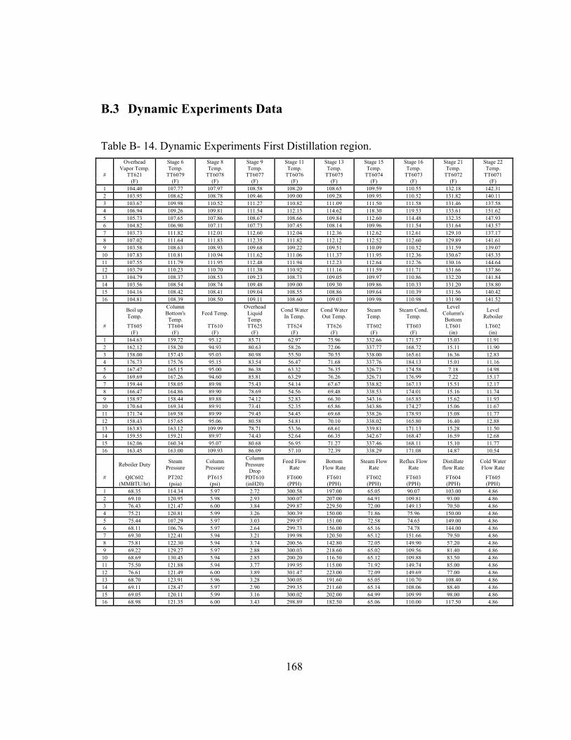
168

B.3 Dynamic Experiments Data

Table B- 14. Dynamic Experiments First Distillation region. Overhead

Vapor Temp. Stage 6 Temp.

Stage 8 Temp.

Stage 9 Temp.

Stage 11 Temp.

Stage 13 Temp.

Stage 15 Temp.

Stage 16 Temp.

Stage 21 Temp.

Stage 22 Temp.

# TT621 TT6079 TT6078 TT6077 TT6076 TT6075 TT6074 TT6073 TT6072 TT6071 (F) (F) (F) (F) (F) (F) (F) (F) (F) (F) 1 104.40 107.77 107.97 108.58 108.20 108.65 109.59 110.55 132.18 142.31 2 103.95 108.62 108.78 109.46 109.00 109.28 109.95 110.52 131.82 140.11 3 103.67 109.98 110.52 111.27 110.82 111.09 111.50 111.58 131.46 137.58 4 106.94 109.26 109.81 111.54 112.13 114.62 118.30 119.53 133.61 151.62 5 105.73 107.65 107.86 108.67 108.66 109.84 112.60 114.48 132.35 147.93 6 104.82 106.90 107.11 107.73 107.45 108.14 109.96 111.54 131.64 143.57 7 103.73 111.82 112.01 112.60 112.04 112.36 112.62 112.61 129.10 137.17 8 107.02 111.64 111.83 112.35 111.82 112.12 112.52 112.60 129.89 141.61 9 103.58 108.63 108.93 109.68 109.22 109.51 110.09 110.52 131.59 139.07 10 107.83 110.81 110.94 111.62 111.06 111.37 111.95 112.36 130.67 145.35 11 107.55 111.79 111.95 112.48 111.94 112.23 112.64 112.76 130.16 144.64 12 103.79 110.23 110.70 111.38 110.92 111.16 111.59 111.71 131.66 137.86 13 104.79 108.37 108.53 109.23 108.73 109.05 109.97 110.86 132.20 141.84 14 103.56 108.54 108.74 109.48 109.00 109.30 109.86 110.33 131.20 138.80 15 104.16 108.42 108.41 109.04 108.55 108.86 109.64 110.39 131.56 140.42 16 104.81 108.39 108.50 109.11 108.60 109.03 109.98 110.98 131.90 141.52

Boil up Temp.


Feed Temp. Overhead

Liquid Temp.

Cond Water In Temp.

Cond Water Out Temp.

Steam Temp.

Steam Cond. Temp.


Level Reboiler

# TT605 TT604 TT610 TT625 TT624 TT626 TT602 TT603 LT601 LT602 (F) (F) (F) (F) (F) (F) (F) (F) (in) (in) 1 164.63 159.72 95.12 85.71 62.97 75.96 332.66 171.57 15.03 11.91 2 162.12 158.20 94.93 80.63 58.26 72.06 337.77 168.72 15.11 11.90 3 158.00 157.43 95.03 80.98 55.50 70.55 338.00 165.61 16.36 12.83 4 176.73 175.76 95.15 83.54 56.47 71.68 337.76 184.13 15.01 11.16 5 167.47 165.15 95.00 86.38 63.32 76.35 326.73 174.58 7.18 14.98 6 169.69 167.26 94.60 85.81 63.29 76.26 326.71 176.99 7.22 15.17 7 159.44 158.05 89.98 75.43 54.14 67.67 338.82 167.13 15.51 12.17 8 166.47 164.86 89.90 78.69 54.56 69.48 338.53 174.01 15.16 11.74 9 158.97 158.44 89.88 74.12 52.83 66.30 343.16 165.85 15.62 11.93 10 170.64 169.34 89.91 73.41 52.35 65.86 343.86 174.27 15.06 11.67 11 171.74 169.58 89.99 79.45 54.45 69.68 338.26 178.93 15.08 11.77 12 158.43 157.65 95.06 80.58 54.81 70.10 338.02 165.80 16.40 12.88 13 163.83 163.12 109.99 78.71 53.36 68.61 339.81 171.13 15.28 11.50 14 159.55 159.21 89.97 74.43 52.64 66.35 342.67 168.47 16.59 12.68 15 162.06 160.34 95.07 80.68 56.95 71.27 337.46 168.11 15.10 11.77 16 163.45 163.00 109.93 86.09 57.10 72.39 338.29 171.08 14.87 10.54

Reboiler Duty Steam Pressure

Column Pressure

Column Pressure

Drop

Feed Flow Rate

Bottom Flow Rate

Steam Flow Rate

Reflux Flow Rate



# QIC602 PT202 PT615 PDT610 FT600 FT601 FT602 FT603 FT604 FT605 (MMBTU/hr) (psia) (psi) (inH20) (PPH) (PPH) (PPH) (PPH) (PPH) (PPH) 1 68.35 114.34 5.97 2.72 300.58 197.00 65.05 90.07 103.00 4.86 2 69.10 120.95 5.98 2.93 300.07 207.00 64.91 109.81 93.00 4.86 3 76.43 121.47 6.00 3.84 299.87 229.50 72.00 149.13 70.50 4.86 4 75.21 120.81 5.99 3.26 300.39 150.00 71.86 75.96 150.00 4.86 5 75.44 107.29 5.97 3.03 299.97 151.00 72.58 74.65 149.00 4.86 6 68.11 106.76 5.97 2.64 299.73 156.00 65.16 74.78 144.00 4.86 7 69.30 122.41 5.94 3.21 199.98 120.50 65.12 151.66 79.50 4.86 8 75.81 122.30 5.94 3.74 200.56 142.80 72.05 149.90 57.20 4.86 9 69.22 129.27 5.97 2.88 300.03 218.60 65.02 109.56 81.40 4.86 10 68.69 130.45 5.94 2.85 200.20 116.50 65.12 109.88 83.50 4.86 11 75.50 121.88 5.94 3.77 199.95 115.00 71.92 149.74 85.00 4.86 12 76.61 121.49 6.00 3.89 301.47 223.00 72.09 149.69 77.00 4.86 13 68.70 123.91 5.96 3.28 300.05 191.60 65.05 110.70 108.40 4.86 14 69.11 128.47 5.97 2.90 299.35 211.60 65.14 108.06 88.40 4.86 15 69.05 120.11 5.99 3.16 300.02 202.00 64.99 109.99 98.00 4.86 16 68.98 121.35 6.00 3.43 298.89 182.50 65.06 110.00 117.50 4.86

169

Feed Feed Feed Distillate Distillate Distillate Bottom Bottom Bottom Level Acc. # Weight Weight Weight Weight Weight Weight Weight Weight Weight LT603 Percent Percent Percent Percent Percent Percent Percent Percent Percent MeOH C5 C6 MeOH C5 C6 MeOH C5 C6 (in) 1 3.67 44.15 52.18 8.65 91.29 0.06 0.87 17.63 81.50 13.02 2 3.49 43.12 53.39 8.73 91.21 0.06 0.02 22.69 77.29 13.12 3 2.98 40.59 56.43 9.98 89.99 0.03 0.00 24.15 75.85 12.97 4 3.94 51.86 44.20 6.33 93.59 0.08 0.00 11.80 88.20 12.96 5 4.00 51.50 44.50 8.10 91.70 0.20 0.00 12.70 87.30 14.09 6 3.90 51.00 45.10 8.30 91.50 0.20 0.00 14.10 85.90 13.26 7 4.47 41.00 54.53 8.09 91.91 0.00 3.19 23.05 73.76 13.02 8 2.77 40.58 56.66 10.16 89.65 0.18 0.04 23.72 76.25 13.17 9 3.13 42.56 54.30 8.46 91.26 0.28 0.16 23.06 76.79 12.87 10 3.11 48.26 48.64 5.20 94.61 0.19 0.04 16.74 83.22 13.03 11 3.05 45.46 51.49 7.15 92.71 0.14 0.06 18.28 81.66 12.96 12 3.02 48.06 48.92 6.33 93.64 0.03 0.00 15.06 84.94 12.87 13 3.23 44.90 51.87 8.62 91.30 0.08 0.15 19.87 79.98 12.99 14 3.14 42.56 54.30 8.46 91.26 0.28 0.15 23.06 76.79 12.93 15 3.75 43.82 52.43 8.49 91.46 0.05 0.00 22.28 77.72 13.09 16 5.41 48.29 46.30 10.17 89.79 0.04 0.00 24.07 75.93 13.03

Table B- 15. Dynamic Experiments Second Distillation region.

Overhead Vapor Temp.

Stage 6 Temp.

Stage 8 Temp.

Stage 9 Temp.

Stage 11 Temp.

Stage 13 Temp.

Stage 15 Temp.

Stage 16 Temp.

Stage 21 Temp.

Stage 22 Temp.

# TT621 TT6079 TT6078 TT6077 TT6076 TT6075 TT6074 TT6073 TT6072 TT6071 (F) (F) (F) (F) (F) (F) (F) (F) (F) (F) 1 110.76 120.22 120.78 122.39 122.34 121.69 122.72 121.44 138.32 157.04 2 118.77 125.89 126.57 129.80 132.54 130.17 129.63 126.12 163.44 165.54 3 104.36 104.43 104.59 104.69 104.36 104.79 105.27 105.48 108.64 116.34 4 104.38 104.43 104.55 104.64 104.29 104.62 104.92 104.98 108.40 115.68 5 114.13 118.57 119.05 120.72 120.53 119.80 120.67 119.83 161.52 164.94 6 103.71 103.79 103.93 103.99 103.63 103.96 104.21 104.32 106.84 108.34 7 103.71 103.79 103.93 103.99 103.63 103.96 104.21 104.20 106.84 108.28 8 104.12 104.25 104.42 104.50 104.19 104.63 105.06 105.24 108.91 119.29 9 103.66 103.74 103.89 103.96 103.59 103.92 104.23 104.26 107.43 111.88 10 103.83 103.91 104.06 104.12 103.74 104.11 104.45 104.53 109.51 128.71 11 103.84 103.93 104.08 104.14 103.77 104.13 104.47 104.55 109.52 128.57 12 103.81 103.90 104.04 104.11 103.73 104.09 104.44 104.52 109.49 128.71 13 104.06 104.16 104.32 104.39 104.07 104.52 105.00 105.21 108.50 114.73 14 104.62 104.72 104.85 104.93 104.56 104.89 105.23 105.28 108.54 112.89 15 104.29 104.37 104.51 104.59 104.22 104.54 104.86 104.94 108.42 115.94 16 104.06 104.16 104.32 104.41 104.09 104.53 105.04 105.30 108.93 118.70

Boil up Temp.

Column Bottom's Temp. Feed Temp.

Overhead Liquid Temp. Reboiler Duty

Feed Flow Rate

Bottom Flow Rate


Reflux Flow Rate

Steam Flow Rate

# TT605 TT604 TT610 TT625 QIC602 FT600 FT601 FT604 FT603 FT602 (F) (F) (F) (F) (MMBTU/hr) (PPH) (PPH) (PPH) (PPH) (PPH) 1 164.35 152.25 94.90 78.89 111.56 300.00 89.55 210.45 148.91 105.07 2 165.85 160.65 94.83 78.20 111.64 300.00 62.56 237.44 99.90 105.07 3 149.96 115.49 94.92 63.15 62.51 300.00 169.27 130.73 74.36 58.05 4 151.10 114.27 95.02 63.02 62.80 300.00 200.09 99.91 100.09 57.99 5 165.28 159.29 95.02 172.96 105.88 300.00 71.47 228.53 99.46 99.99 6 114.10 107.65 94.90 125.10 60.98 300.00 199.88 100.12 99.97 55.01 7 114.10 107.65 94.90 125.10 60.98 300.00 199.88 100.12 99.97 55.01 8 155.12 120.53 94.89 66.24 80.09 300.00 127.20 172.80 112.98 75.02 9 144.35 112.10 95.04 66.44 62.76 300.00 184.59 115.41 99.80 57.96 10 158.63 126.11 94.91 67.43 61.99 200.00 90.41 109.59 98.60 57.90 11 158.46 125.64 94.97 67.46 62.04 200.00 90.15 109.85 99.54 57.89 12 158.64 126.30 94.92 67.41 62.06 200.00 136.97 63.03 97.67 57.74 13 149.74 115.03 111.71 68.00 62.89 350.00 199.92 150.08 100.64 58.02 14 146.23 112.44 94.96 62.98 62.38 350.00 239.95 110.05 100.22 57.61 15 151.60 114.46 95.10 63.21 62.88 300.00 188.46 111.54 100.07 57.99 16 154.96 120.11 113.13 68.68 62.31 300.00 149.97 150.03 100.41 57.93

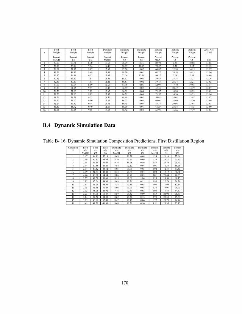
170

Feed Feed Feed Distillate Distillate Distillate Bottom Bottom Bottom Level Acc. # Weight Weight Weight Weight Weight Weight Weight Weight Weight LT603

Percent Percent Percent Percent Percent Percent Percent Percent Percent MeOH C5 C6 MeOH C5 C6 MeOH C5 C6 (in) 1 37.99 53.71 8.30 15.56 76.09 8.35 89.70 0.28 10.02 13.02 2 36.18 53.89 9.94 19.46 68.09 12.45 99.57 0.31 0.12 13.12 3 39.01 51.82 9.17 12.63 87.30 0.07 60.87 22.98 16.15 12.97 4 41.59 48.92 9.49 11.69 88.30 0.01 61.27 24.58 14.15 12.96 5 35.57 54.91 9.52 15.05 72.06 12.90 99.27 0.04 0.69 14.09 6 42.43 49.67 7.91 11.41 88.57 0.02 59.45 28.34 12.21 13.26 7 42.43 49.67 7.91 11.41 88.57 0.02 59.45 28.34 12.21 13.02 8 33.67 57.64 8.69 12.60 87.35 0.05 62.97 17.10 19.93 13.17 9 39.28 51.16 9.57 13.43 86.55 0.02 57.35 28.47 14.19 12.87 10 39.20 51.60 9.12 13.65 86.31 0.04 71.57 10.20 18.23 13.03 11 39.20 51.60 9.12 13.65 86.31 0.04 71.57 10.20 18.23 12.96 12 38.76 51.71 9.53 11.50 88.48 0.02 50.42 35.62 13.97 12.87 13 39.90 51.00 9.10 13.23 86.73 0.03 60.01 24.69 15.30 12.99 14 41.24 49.32 9.44 13.51 86.45 0.05 55.37 30.98 13.64 12.93 15 41.59 48.92 9.49 11.69 88.30 0.01 61.27 24.58 14.15 13.09 16 40.01 50.95 9.05 13.54 86.42 0.04 65.95 16.66 17.39 13.03

B.4 Dynamic Simulation Data

Table B- 16. Dynamic Simulation Composition Predictions. First Distillation Region Condition Feed Feed Feed Distillate Distillate Distillate Bottom Bottom Bottom

# w% w% w% w% w% w% w% w% w% MeOH C5 C6 MeOH C5 C6 MeOH C5 C6 1 3.67 44.15 52.18 8.63 91.29 0.08 1.24 21.10 77.66 2 3.49 43.12 53.39 8.70 91.21 0.09 1.33 23.22 75.45 3 2.98 40.59 56.43 9.16 89.98 0.86 0.87 23.70 75.43 4 3.94 51.86 44.20 7.84 92.12 0.04 0.01 11.33 88.66 5 3.97 51.52 44.52 8.05 91.91 0.03 0.02 12.45 87.53 6 3.99 50.61 45.40 8.33 91.63 0.04 0.02 13.17 86.81 7 4.46 41.00 54.54 8.06 91.91 0.03 3.01 20.44 76.55 8 2.77 40.58 56.66 8.55 89.61 1.84 0.29 19.56 80.15 9 3.13 42.56 54.30 8.63 91.26 0.11 0.90 22.74 76.36 10 3.11 48.26 48.64 7.58 92.39 0.03 0.00 17.66 82.34 11 3.05 45.46 51.49 8.06 91.91 0.03 0.30 19.97 79.73 12 3.02 48.06 48.92 7.16 92.81 0.03 0.00 15.43 84.57 13 3.23 44.90 51.87 8.59 91.32 0.09 0.69 22.94 76.37 14 3.14 42.56 54.30 8.62 91.26 0.12 0.98 23.38 75.64 15 3.75 43.82 52.43 8.47 91.47 0.06 1.77 23.79 74.44 16 5.41 48.29 46.30 8.69 91.21 0.10 3.51 23.35 73.15

171

Table B- 17. Dynamic Simulation Composition Predictions. Second Distillation Region

Condition Feed Feed Feed Distillate Distillate Distillate Bottom Bottom Bottom # w% w% w% w% w% w% w% w% w% MeOH C5 C6 MeOH C5 C6 MeOH C5 C6 1 37.99 53.71 8.30 16.01 76.56 7.43 89.64 0.02 10.34 2 36.18 53.89 9.94 19.55 68.00 12.45 99.29 0.32 0.39 3 39.01 51.82 9.17 10.76 87.99 1.25 60.83 23.88 15.29 4 41.59 48.92 9.49 9.97 89.39 0.63 57.38 28.71 13.91 5 35.57 54.91 9.52 15.43 72.08 12.49 99.98 0.00 0.02 6 42.43 49.67 7.91 9.87 89.61 0.52 58.73 29.66 11.61 7 42.43 49.67 7.91 9.87 89.61 0.52 58.73 29.66 11.61 8 33.67 57.64 8.69 11.12 87.20 1.68 64.31 17.48 18.21 9 39.27 51.16 9.57 10.15 89.08 0.77 57.48 27.45 15.07 10 39.28 51.60 9.12 10.97 87.42 1.61 73.59 8.18 18.23 11 39.28 51.60 9.12 10.97 87.42 1.61 73.59 8.18 18.23 12 38.76 51.71 9.53 9.97 89.39 0.63 52.01 34.37 13.62 13 41.60 48.90 9.50 10.94 87.60 1.46 64.61 19.85 15.54 14 41.24 49.32 9.44 10.64 89.31 0.05 55.27 30.98 13.75 15 41.59 48.92 9.49 10.20 89.00 0.80 60.17 25.20 14.63 16 40.00 50.95 9.05 11.12 87.20 1.68 68.89 14.69 16.43

Table B- 18. Experimental data material balance error. Second Distillation Region Mass Balance Difference

MeOH C5 C6 Condition

#

Feed w%

MeOH

Feed w% C5

Feed w% C6

Distillate w%

MeOH

Distillate w% C5

Distillate w% C6

Bottom w%

MeOH

Bottom w% C5

Bottom w% C6 (PPH) (PPH) (PPH)

1 37.99 53.71 8.30 15.56 76.09 8.35 89.70 0.28 10.02 0.88 0.75 -1.63 2 36.18 53.89 9.94 19.46 68.09 12.45 99.57 0.31 0.12 0.04 -0.21 0.17 3 39.01 51.82 9.17 12.63 87.30 0.07 60.87 22.98 16.15 -2.51 2.44 0.08 4 41.59 48.92 9.49 11.69 88.30 0.01 61.27 24.58 14.15 -9.50 9.36 0.13 5 35.57 54.91 9.52 15.05 72.06 12.89 99.27 0.04 0.69 1.39 0.02 -1.40 6 42.43 49.67 7.91 11.41 88.57 0.02 59.45 28.34 12.21 -2.98 3.68 -0.70 7 42.43 49.67 7.91 11.41 88.57 0.02 59.45 28.34 12.21 -2.98 3.68 -0.70 8 33.67 57.64 8.69 12.60 87.35 0.05 62.97 17.10 19.93 -0.84 0.22 0.63 9 39.28 51.16 9.57 13.43 86.55 0.02 57.35 28.47 14.19 -3.53 1.05 2.49 10 39.20 51.60 9.20 13.65 86.31 0.04 71.57 10.20 18.23 -1.26 -0.60 1.87 11 39.20 51.60 9.20 13.65 86.31 0.04 71.57 10.20 18.23 -1.11 -0.80 1.92 12 38.76 51.71 9.53 11.50 88.48 0.02 50.42 35.62 13.97 1.21 -1.13 -0.08 13 39.90 51.00 9.10 13.23 86.73 0.04 60.01 24.69 15.30 -0.18 -1.01 1.19 14 41.24 49.32 9.44 13.51 86.45 0.05 55.37 30.98 13.65 -3.39 3.15 0.25 15 41.59 48.92 9.49 11.69 88.30 0.01 61.27 24.58 14.15 -3.73 1.96 1.78 16 40.01 50.95 9.05 13.54 86.42 0.04 65.95 16.66 17.39 0.79 -1.81 1.01

172

Appendix C. NRTL Model for Multicomponent Systems

For multicomponent systems, the NRTL equation for the molar Excess Gibbs

energy is

∑

∑∑

=

=

=

= m

llli

m

jjjijim

ii

Em

xG

xGx

RTG

1

1

1

τ

( )ijijijG τα−= exp

The activity coefficient for a component i is given by

∑∑

∑

∑∑

∑=

=

=

==

=

⎟⎟⎟⎟

⎠

⎞

⎜⎜⎜⎜

⎝

⎛

−+=m

jm

llli

m

rririr

ijm

lllj

ijjm

llli

m

jjjiji

i

xG

Gx

xG

Gx

xG

xG

1

1

1

11

1lnτ

ττ

γ

There are three parameters for each pair of components, ijτ , jiτ , and jiij αα = ,

and no new parameters for interactions on three different species.

173

Appendix D. 6” Distillation Column Start-Up Standard Operation

Procedure

1. Enable the feed pump [P600] and start it manually. Be sure the gate valve for

the recycle back to the feed tank is open so the sampling system will work.

2. Put the sampling devices, to enable the recycle loop for the bottom. Take

sample to determine feed values.

3. Turn on chilled water pump [P-101CW] and make sure the chilled water flow

meter [FT605] reads between 5-7 gpm.

4. Determine whether 18” Distillation Column needs to be isolated from the

steam flow.

5. Set pressure control valve output [PC615] to 0 psig (to stop wasting nitrogen)

and put the controller in AUTO. The vent valve will open to its maximum

allowable point during startup.

6. Put all flow control loops in MANUAL and set the outputs to 0%.

a. FC600

b. FC601

c. FC602

d. FC603

e. FC604

174

f. TC610

7. Master loops for level control in the accumulator [LC603] and the column

[LC601] may be left in AUTO. LC603 should be set to 13 inches of level and

LC601 should be set to 15 inches of level.

8. Open ball valves around FCV600 and FCV601, bottom of the tank, two

bottoms valves (before the filter). Follow the flow path.

9. Open nitrogen line (ball valve) and set backpressure on feed tank to 20 psig.

10. Make sure the purges are set between 20 – 30.

11. Open the feed flow valve to 50 %. After reaching a stable flow, set the feed

flow controller [FC600] to AUTO and provide a set point of 300 lb/hr.

12. Observe the column level [LT601]. When it reaches 13 inches, check the

level in the glass. If it is above the middle, start the bottom pump [P601].

13. Open the bottom valve [FC601] a little, to make sure there is a flow, hence all

ball valves are open.

14. After this check, if there is a level of 15 inch in the column, close the valves

[FC600] and [FC601].

15. Recheck if the other columns need to be isolated. (Steve and Chris)

16. Check that the isolation valve is open.

17. Gradually open steam gate valve located on the wall outside the SRP Control

Room. Make sure the condensate return line is open as well (next to steam

line).

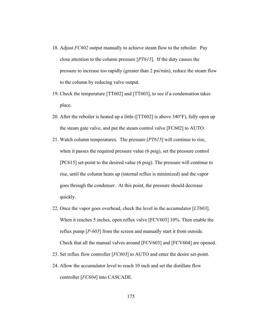
175

18. Adjust FC602 output manually to achieve steam flow to the reboiler. Pay

close attention to the column pressure [PT615]. If the duty causes the

pressure to increase too rapidly (greater than 2 psi/min), reduce the steam flow

to the column by reducing valve output.

19. Check the temperature [TT602] and [TT603], to see if a condensation takes

place.

20. After the reboiler is heated up a little ([TT602] is above 340°F), fully open up

the steam gate valve, and put the steam control valve [FC602] to AUTO.

21. Watch column temperatures. The pressure [PT615] will continue to rise,

when it passes the required pressure value (6 psig), set the pressure control

[PC615] set-point to the desired value (6 psig). The pressure will continue to

rise, until the column heats up (internal reflux is minimized) and the vapor

goes through the condenser. At this point, the pressure should decrease

quickly.

22. Once the vapor goes overhead, check the level in the accumulator [LT603].

When it reaches 5 inches, open reflux valve [FCV603] 10%. Then enable the

reflux pump [P-603] from the screen and manually start it from outside.

Check that all the manual valves around [FCV603] and [FCV604] are opened.

23. Set reflux flow controller [FC603] to AUTO and enter the desire set-point.

24. Allow the accumulator level to reach 10 inch and set the distillate flow

controller [FC604] into CASCADE.

176

25. Set the feed flow controller [FC600] to AUTO and set the set-point to 300

lb/hr.

26. Set the bottoms flow controller [FC601] to CASCADE and set the set-point

[LC602] to 15 inches. After the level set point for the bottom column is

reached, close the bottom sample loop, to achieve a greater flowrate in the

bottom.

27. Check the level of the column. If the bottom flow rate is not able to control

the level in the bottom of the column, the steam flow may need to be adjusted.

(increase if level is too high, decrease if level is too low).

28. Check the output limits for the pre-heater. Make sure the output high limit is

around 75%. Set the feed pre-heater controller [TC610] to AUTO and input

the desire set point.

29. Allow the column to reach a steady state (approximately 4 hours).

177

Appendix E. 6” Distillation Column Shut Down Standard

Operation Procedure

1. Set the steam flow controller [FC602] to MANUAL and set the valve position

to 0% [FV602]. Close the steam gate valve or isolate the column from the

steam-flow, if steam is needed in another process.

2. Set the feed flow controller [FC600] to MANUAL and set the valve position

to 0% [FV600].

3. Set the distillate flow controller [FC604] to MANUAL and set the valve

position to 0% [FV604].

4. Set the reflux flow controller [FC603] to MANUAL and set the valve position

to 50% [FV603].

5. Set the bottom flow controller [FC601] to MANUAL and set the valve

position to 100% [FV601].

6. Set the Column pressure controller to the set-point of 0 psig

7. Monitor the accumulator level and the reflux flow rate. When both are less

than zero turn off the overhead pump P603.

8. Monitor columns level and bottoms flow rate, when both indicate less than

zero turn the bottoms pump P601 off.

9. Turn off feed pump P600 .

178

10. Close manual valves after control valves (FV600, FV601, FV603, FV604).

11. Close manual valves in bottoms loop (pump recycle, column line, filter

isolation, feed tank return).

12. Stop cold water pump.

179

Bibliography [1] Abouelhassan M., Simard A. (2003). The Scoop on Tray Efficiency. Distillation

Series, Aspentech Documentation. [2] Åström K.J, Wittenmark B. Adaptive Control (1995). Addison-Wesley

Publishing Co. Boston, MA. [3] Baur, R., Taylor, R., Krishna, R. and Copati, J. A. (1999). Influence of mass

transfer in distillation of mixtures with a distillation boundary, Trans IchemE, Part A, Chem Eng Res Des. 77, 561–565.

[4] Bekiaris, N. and M. Morari (1996). Multiple Steady States in Distillation: 1=1 Predictions, Extensions, and Implications for Design, Synthesis, and Simulation. Ind. End. Chem. Res .35, 4264–4280.

[5] Bekiaris, N., G.A. Meski, G.A. Raudu and M.Morari (1993).Multiple Steady States in Homogeneous Azeotropic Distillation. Ind. Eng. Chem. Res. 32(9), 2023–2038.

[6] Bekiaris, N., G.A. Meski, G.A. Raudu and M.Morari (1996).Multiple Steady States in Heterogeneous Azeotropic Distillation. Ind. Eng. Chem. Res. 35(1), 207-27.

[7] Billet, R., Schultes, M. (1999). Prediction of mass transfer columns with dumped and arranged packings. Updated summary of the calculation method of Billet and Schultes. Chemical Engineering Research and Design, 77(A6), 498-504.

[8] Bequette B.W. and Edgar T.F. (1989), Non-interacting control system design methods in distillation. Computers Chem. Eng. 13, pp. 641–650.

[9] Bristol E. (1966). On a new measure of interaction for multivariable process control. IEEE Trans. Automat. Contr., vol. 11, p. 133.

[10] Bulletin DC-11. (1977). Norton Co., Akron, OH. [11] Buckley, Page S., Luyben, William L., and Shunta, Joseph P. (1985) Design of

Distillation Column Control Systems. Research Triangle Park, N.C., Edward Arnold, Instrument Society of America, 1985.

[12] Chien, I-Lung; Chao, Huan-Yi; Teng, Yao-Pin. Design and control of a complete heterogeneous azeotropic distillation column system. (2003) Computer-Aided Chemical Engineering, 15B (Process Systems Engineering 2003, Part B), 760-765.

[13] Chien, I-L.; Wang, C. J.; Wong, D. S. H.; Lee, C.-H.; Cheng, S.-H.; Shih, R. F.; Liu, W. T.; Tsai, C. S. (2000). Experimental investigation of conventional control strategies for a heterogeneous azeotropic distillation column. Journal of Process Control, 10(4), 333-340.

[14] Chien, I-Lung; Zeng, Kai-Luen; Chao, Huan-Yi. (2004). Design and Control of a Complete Heterogeneous Azeotropic Distillation Column System. Ind. Eng. Chem. Res. 43(9), 2160-2174.

180

[15] Doherty, Michael F.; Caldarola Glenn A. (1985). Sequencing of Columns for Azeotropic and Extractive Distillation. Ind. Eng. Chem. Fundam. 24, 474-485.

[16] Doherty, Michael F.; Malone M.F. (2001). Conceptual Design of Distilaltion Systems. McGraw-Hill, New York.

[17] De Villiers, Waldo E.; French, Raymond N.; Koplos, George J.. (2002). Navigate phase equilibria via residue curve maps. Chemical Engineering Progress. 98(11), 66-71.

[18] Elliott, Richard and Lira Carl T. (1999). Introductory Chemical Engineering Thermodynamics. Upper Saddle River, N.J.: Prentice Hall PTR.

[19] Hilmen, E.K. (2000). Separation of Azeotropic Mixtures: Tools for Analysis and Studies on Batch Distillation Operation. PhD thesis. Norwegian University of Science and Technology, Department of Chemical Engineering.

[20] Joseph, B.; Brosilow, C. B.; Howell, J. C.; Kerr, W. R. D. (1975) Multi-temps give better control. Hydrocarbon Processing (1966-2001), 55(3), 127-31.

[21] King, C. J. (1980). Separation Processes. McGraw-Hill Company. [22] Kiva V.N., Hilmen E.K. and Skogestad S. (2003). Azeotropic Phase Equilibrium

Diagrams: A Survey. Chemical Engineering Science, 58, 1903-1953. [23] Krishna, R and Taylor, R. (1985) A Nonequilibrium Stage Model of

Multicomponent Separation Processes. Part I: Model Description and Method of Solution, AIChE J., 31(3), 449.

[24] Krishna, R and Taylor, R. (1985) A Nonequilibrium Stage Model of Multicomponent Separation Processes. Part II: Comparison with Experiment, AIChE J., 31(3), 456.

[25] Krishna, R and Taylor, R. (1985) Simulation of Packed Distillation and Absorption Columns, Ind. Eng. Chem. Process Des. Dev., 24(3), 513.

[26] Kumar, S.; Wright, J. D.; Taylor, P. A. (1984). Modeling and dynamics of an extractive distillation column. Canadian Journal of Chemical Engineering. 62(6), 780-9.

[27] Kurooka, Taketoshi; Yamashita, Yuh; Nishitani, Hirokazu; Hashimoto, Yoshihiro; Yoshida, Masatoshi; Numata, Motoki.(2000).Dynamic simulation and nonlinear control system design of a heterogeneous azeotropic distillation column. Computers & Chemical Engineering 24(2-7), 887-892.

[28] Luyben, William L. (2005). Guides for the Selection of Control Structures for Ternary Distillation Columns. Industrial & Engineering Chemistry Research, 44(18), 7113-7119.

[29] Luyben, William L.; Vinante, Carols D. (1972). Experimental studies of distillation decoupling. Kemian Teollisuus, 29(8), 499-514.

[30] Maciel, M. R. Wolf; Brito, R. P. (1995). Evaluation of the dynamic behavior of an extractive distillation column for dehydration of aqueous ethanol mixtures. Computers & Chemical Engineering. 19(Suppl., European Symposium on Computer Aided Process Engineering--5), S405-S408.

181

[31] Mathijssen, A. (2005). Experimental validation of the steady-state simulation of an industry-sized distillation column, Studienarbeit, Lehrstuhl für Prozesstechnik, RWTH Aachen.

[32] McAvoy, T. (1983). Interaction Analysis, ISA, Research Triangle Park. [33] Müller, D.; Marquardt, W. (1997). Experimental Verification of Multiple Steady

States in Heterogeneous Azeotropic Distillation. Ind. Eng. Chem. Res. 36, 5410-5418

[34] Onda, K., Takeuchi, H., and Okumoto, Y.. (1968) "Mass Transfer Coefficients between Gas and Liquid Phases in Packed Columns," J. Chem. Eng., Japan. 1, 56.

[35] Parrish, J. R.; Brosilow, C. B. Nonlinear inferential control. (1982) AIChE Journal (1988), 34(4), 633-44.

[36] Patke, N. G.; Deshpande, P. B. (1982). Experimental evaluation of the inferential system for distillation control. Chemical Engineering Communications, 13(4-6), 343-59.

[37] Peng, JJ. (2003). Modeling and Control of Packed Reactive Distillation Columns. PhD thesis, University of Texas at Austin.

[38] Renon H., Prausnitz J. M. (1968). Local compositions in thermodynamics excess functions for liquid mixtures. AIChE J. 14, 135-144.

[39] Qin, S. J. and Badgwell, T. A. (1997). An overview of industrial model predictive control technology. In Proc. Chemical Process Control - V, 232–256.

[40] Redlich, O. and Kwong, J.N.S. (1949). On the Thermodynamics of Solutions. Chem. Rev. 44, 233-244.

[41] Repke, Jens-Uwe; Villain, Olivier; Wozny, Gunter. (2004). A nonequilibrium model for three-phase distillation in a packed column: modelling and experiments. Computers & Chemical Engineering. 28(5), 775-780.

[42] Robbins, Lanny A. (1991). Improve pressure-drop prediction with a new correlation. Dow Chem. Co., USA. Chemical Engineering Progress. 87(5), 87-91.

[43] Rovaglio, M.; Faravelli, T.; Gaffuri, P.; Di Palo, C.; Dorigo, A. (1995). Controllability and operability of azeotropic heterogeneous distillation systems. Computers & Chemical Engineering. 19(Suppl., European Symposium on Computer Aided Process Engineering--5), S525-S530.

[44] Rueda, L.M.; Edgar, T.F.; Eldridge R.B. (2004). On-line Parameter Estimation and Control for a Pilot Scale Distillation Column, AIChE Annual Meeting, Austin,TX.

[45] Seader, J. D. (1985). The B.C. (before computers) and A.D. of equilibrium-stage operations. Chemical Engineering Education, 19(2), 88-103.

[46] Seader, J. D. and Henley, E. J. (1998). Separation Process Principles. Wiley, New York.

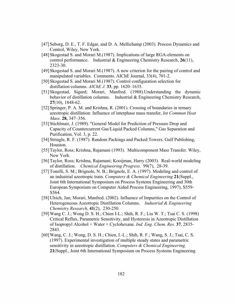
182

[47] Seborg, D. E., T. F. Edgar, and D. A. Mellichamp (2003). Process Dynamics and Control, Wiley, New York.

[48] Skogestad S. and Morari M.(1987). Implications of large RGA-elements on control performance. Industrial & Engineering Chemistry Research, 26(11), 2323-30.

[49] Skogestad S. and Morari M.(1987). A new criterion for the pairing of control and manipulated variables. Comments. AIChE Journal, 33(4), 701-2.

[50] Skogestad S. and Morari M.(1987). Control configuration selection for distillation columns. AIChE J. 33, pp. 1620–1635.

[51] Skogestad, Sigurd; Morari, Manfred. (1988).Understanding the dynamic behavior of distillation columns. Industrial & Engineering Chemistry Research, 27(10), 1848-62.

[52] Springer, P. A. M. and Krishna, R. (2001). Crossing of boundaries in ternary azeotropic distillation: Influence of interphase mass transfer, Int Commun Heat Mass. 28, 347–356.

[53] Stichlmair, J. (1989). "General Model for Prediction of Pressure Drop and Capacity of Countercurrent Gas/Liquid Packed Columns," Gas Separation and Purification, Vol. 3, p. 22.

[54] Stringle, R. F. (1987). Random Packings and Packed Towers. Gulf Publishing, Houston.

[55] Taylor, Ross; Krishna, Rajamani (1993). Multicomponent Mass Transfer. Wiley, New York.

[56] Taylor, Ross; Krishna, Rajamani; Kooijman, Harry (2003). Real-world modeling of distillation. Chemical Engineering Progress. 99(7), 28-39.

[57] Tonelli, S. M.; Brignole, N. B.; Brignole, E. A. (1997). Modeling and control of an industrial azeotropic train. Computers & Chemical Engineering 21(Suppl., Joint 6th International Symposium on Process Systems Engineering and 30th European Symposium on Computer Aided Process Engineering, 1997), S559-S564.

[58] Ulrich, Jan; Morari, Manfred. (2002). Influence of Impurities on the Control of Heterogeneous Azeotropic Distillation Columns. Industrial & Engineering Chemistry Research, 41(2), 230-250.

[59] Wang C. J.; Wong D. S. H.; Chien I-L.; Shih, R. F.; Liu W. T.; Tsai C. S. (1998) Critical Reflux, Parametric Sensitivity, and Hysteresis in Azeotropic Distillation of Isopropyl Alcohol + Water + Cyclohexane. Ind. Eng. Chem. Res. 37, 2835-2843.

[60] Wang, C. J.; Wong, D. S. H.; Chien, I.-L.; Shih, R. F.; Wang, S. J.; Tsai, C. S. (1997). Experimental investigation of multiple steady states and parametric sensitivity in azeotropic distillation. Computers & Chemical Engineering. 21(Suppl., Joint 6th International Symposium on Process Systems Engineering

183

and 30th European Symposium on Computer Aided Process Engineering, 1997), S535-S540.

[61] Weber, Richard; Mosler, Henry A. (1973) Temperature control of distillation. (Esso Research and Engineering Co.). U.S. 7 PP.

[62] Widagdo, S. and W.D. Seider (1990). Journal Review: Azeotropic Distillation. AIChE J. 42(1), 96–128.

[63] Witcher M.F., McAvoy T.J. (1977). Interacting control systems: steady-state and dynamic measurement of interaction. ISA Trans., 16 (3), 35-41.

[64] Yamamoto, Shoushi; Yoneda, Minoru; Yabuki, Yasuaki. (2003).The control of heterogeneous azeotropic distillation column in industry considering entrainer ratio in reflux. Computer-Aided Chemical Engineering. 15B(Process Systems Engineering 2003, Part B), 1094-1099.

[65] Yu, Cheng Ching; Luyben, William L. (1984). Use of multiple temperatures for the control of multicomponent distillation columns. Industrial & Engineering Chemistry Process Design and Development , 23(3), 590-7

184

Vita

Lina María Rueda Velandia was born on July 9, 1977 in Barrancabermeja,

Santander, Colombia as the youngest of four children of Gladys Velandia de Rueda

and Guillermo Rueda Rueda. Lina attended high school in her home town and

graduated from El Colegio El Rosario in December 1994 after receiving the national

prize Andrés Bello for being one of the best high school graduates in the country.

On January 1995, Lina began her engineering studies at Pontificia Universidad

Javeriana (PUJ) where she received her bachelor’s degree in Electrical Engineering in

May 2000. Her graduate project was nominee to best graduate project. In 1999 when

she was still attending school, Lina worked as support engineer for the Y2K transition

in the Colombian National Petroleum Company (ECOPETROL) and in 2000 she

worked as designed engineer for the Colombian-Italian company Tipiel S.A. Later

that year she enrolled PUJ as instructor of different Electrical Engineering courses

and laboratory assistant. In spring 2002, Lina moved to Austin, TX and entered the

graduate school at The University of Texas at Austin. She received a Master of

Science degree in Engineering from The University of Texas at Austin in May 2004.

Upon graduation with her PhD degree, she has accepted employment with Pavilion

Technologies in Austin, TX.

Permanent Address: 1632 W 6th St. Apt. K Austin, TX. 78703

This dissertation was typed by the author.

Date post:	01-Dec-2021
Category:	Documents
Upload:	others
View:	1 times
Download:	0 times

Copyright by Lina María Rueda 2005

Documents