Copyright By Phillip Wingate Vaughan 2009

Copyright

By

Phillip Wingate Vaughan

2009

The Dissertation Committee for Phillip Wingate Vaughan

certifies that this is the approved version of the following dissertation:

Confirmatory Factor Analysis with Ordinal Data:

Effects of Model Misspecification and Indicator Nonnormality on

Two Weighted Least Squares Estimators

Committee:

____________________________________

S. Natasha Beretvas, Supervisor

____________________________________

Samuel D. Gosling

____________________________________

William R. Koch

____________________________________

Keenan A. Pituch

____________________________________

Arthur Sakamoto




by

Phillip Wingate Vaughan, B.A., M.A.

Dissertation

Presented to the Faculty of the Graduate School of

The University of Texas at Austin

in Partial Fulfillment

of the Requirements

for the Degree of

Doctor of Philosophy

The University of Texas at Austin

August 2009

Dedicated to my parents,

who have always valued education immensely,

and my Basset hound Lucky,

who is pleasantly ineducable.

v

Acknowledgements

I find myself bumping up against the absolute deadline to upload the dissertation,

and I haven’t yet written the acknowledgments. My brain is tired and hurt. First, I’d like

to thank the members of my committee. I picked each of you because you taught at least

one course that I really liked, and my intuitions told me that you were solid people. I am

always right about these things. More specifically, thanks to Art Sakamoto for teaching a

great regression-intensive class that gave me a new appreciation for net effects at a time

when I really needed to know these things. Thanks to Bill Koch for teaching a lot of

foundational classes that I took, and also for employing me as a TA on many occasions.

Keenan Pituch very effectively taught a valuable and informative course on HLM that

was one of the capstones of my formal education. It has also been a pleasure to work with

him on the SeniorWISE project. Keenan, thanks also for your mentorship as I pursue an

academic career. I really appreciate it. Before Sam Gosling came to UT, there was no one

(that I’m aware of) to teach the Personality course I took from him. I am continually

inspired by his personal blend of industriousness and creativity, and he wrote a great

book, too. Sam, thanks also for pushing me to submit some papers and for inviting me to

the Social-Personality talks in the Psych Department. Tasha Beretvas, my dissertation

adviser, taught wonderful courses in both factor analysis and meta analysis. Tasha, thank

you also for insisting that I do an actual simulation study for my dissertation. I was cool

to the idea at first, but it has been a great experience. Thank you also for pushing me to

submit the APA poster a while back, and for being so effective at working with me.

vi

Thanks to Graham McDougall and Heather Becker in the UT-Austin School of

Nursing. Working with you guys, Taylor Acee, Carol Delville, and Keenan on the

SeniorWISE project has been fun, educational, and I really enjoy the camaraderie we

have established. All the pubs aren’t bad, either. Thanks also to Adama Brown in

Nursing. Working in the Cain Center gave me great experience in research and stats

consulting, and I had a great time too.

There’s not much of a theme to this paragraph: Grad school is nothing without

making some good buddies, and so I am happy to have met Rick Sperling and Taylor.

Diana, thanks for the stimulating talks over lunch. Thanks also to Virginia Stockwell, the

Graduate Coordinator for the UT-Austin Department of Educational Psychology, for

being so extremely competent and helpful. Virginia, you are very good at your job. I

would also like to acknowledge the well-taught Structural Equation Modeling course that

I took from the now-departed-from-UT Laura Stapleton. Well done.

My parents deserve special thanks. They have always valued education. For that

matter, thanks for having only one child. And thanks for not questioning me when I spent

a long time in grad school. It was worth it. Dad, thank you and Theresa for understanding

my pursuit of learning, and Mom, thanks for some very timely dog sitting as I worked on

this dissertation (not that you don’t also understand learning). Thanks also to my long-

time buddies Mark and Brad. My life is definitely richer for knowing you guys.

My brain is tired now. Sorry if I left you out. I will make it up to you. Thanks to

my kind dog Lucky. Thanks also to my future wife. You have great taste in men.

vii




Publication No. ____________

Phillip Wingate Vaughan, Ph.D.

The University of Texas at Austin, 2009

Supervisor: S. Natasha Beretvas

Full weighted least squares (full WLS) and robust weighted least squares (robust

WLS) are currently the two primary estimation methods designed for structural equation

modeling with ordinal observed variables. These methods assume that continuous latent

variables were coarsely categorized by the measurement process to yield the observed

ordinal variables, and that the model proposed by the researcher pertains to these latent

variables rather than to their ordinal manifestations.

Previous research has strongly suggested that robust WLS is superior to full WLS

when models are correctly specified. Given the realities of applied research, it was

critical to examine these methods with misspecified models. This Monte Carlo simulation

study examined the performance of full and robust WLS for two-factor, eight-indicator

viii

confirmatory factor analytic models that were either correctly specified, overspecified, or

misspecified in one of two ways. Seven conditions of five-category indicator distribution

shape at four sample sizes were simulated. These design factors were completely crossed

for a total of 224 cells.

Previously findings of the relative superiority of robust WLS with correctly

specified models were replicated, and robust WLS was also found to perform better than

full WLS given overspecification or misspecification. Robust WLS parameter estimates

were usually more accurate for correct and overspecified models, especially at the

smaller sample sizes. In the face of misspecification, full WLS better approximated the

correct loading values whereas robust estimates better approximated the correct factor

correlation. Robust WLS chi-square values discriminated between correct and

misspecified models much better than full WLS values at the two smaller sample sizes.

For all four model specifications, robust parameter estimates usually showed lower

variability and robust standard errors usually showed lower bias.

These findings suggest that robust WLS should likely remain the estimator of

choice for applied researchers. Additionally, highly leptokurtic distributions should be

avoided when possible. It should also be noted that robust WLS performance was

arguably adequate at the sample size of 100 when the indicators were not highly

leptokurtic.

ix

Table of Contents

Chapter I: Introduction…………………………………………………………………….1

Chapter II: Review of the Literature………………………………………………………5

Confirmatory Factor Analysis……………………………………………………13

Estimation Methods for Continuous Data………………………………………..15

Normal Theory Estimators…………………………………………….…15

The Asymptotically Distribution Free Estimator………………………...21

Satorra-Bentler Scaling…………………………………………………..25

Maximum Likelihood, Satorra-Bentler Scaling and Asymptotically

Distribution Free Estimation with Misspecified Models………………...27

Estimation Methods for Ordered Categorical Data……………………………...30

Normal Theory Estimators with Ordered Categorical Data……………..35

Satorra-Bentler Correction with Ordered Categorical Data……………...42

Polychoric Correlations………………………………………………….43

Polychoric Correlations with Normal Theory Estimators……………….47

Full Weighted Least Squares Estimation…………………………….…..51

Robust Weighted Least Squares Estimation……………………….…….60

Full WLS and Robust WLS Empirically Compared……………………..63

Chi-square statistics……………………………………………...65

Parameter estimates……………………………………………...69

Standard errors…………………………………………………...73

x

Empirical standard deviations of factor loadings………………...75

Summary of Flora and Curran (2004)……………………………78

Statement of the Problem………………………………………………………...78

Purpose of the Study……………………………………………………………..82

Chapter III: Method………………………………………..…………………………….83

Population Model………………………………………………………………...83

Design Factors…………………………………………………………………...85

Distributions of Observed Variables……………………………………..86

Model Specifications…………………………………………………….88

Design Summary…………………………………………………………90

Data Generation………………………………………………………………….90

Outcomes of Interest……………………………………………………………..92

Chi-Square Statistics………………………………………………….….93

Estimated Standard Errors……………………………………………….98

Empirical Standard Errors…………………………………….………….98

Chapter IV: Results………………………………………………………………………99

Nonconvergent and Inadmissible Solutions……………………………………...99

Expected Values of Chi-Square for Misspecified Models……………………...103

Model Chi-Square Values………………………………………………………106

Relative Bias of Chi-square Values…………………………………….106

Proportions of Statistically Significant Chi-Square Values…………….112

Relative Bias of Parameter Estimates…………………………………………..117

xi

Uncomplicated Loading λ1,1……………………………………………117

Complicated Loading λ1,4………………………………………………123

True Cross Loading λ1,5………………………………………………...129

Superfluous Cross Loading λ2,3………………………………………...132

Factor Correlation ψ…………………………………………………….135

Mean Absolute Value of Relative Bias for All Estimated Parameters…140

Precision of Parameter Estimates……………………………………………….145




Superfluous Cross Loading λ2,3………………………………………...158


Standard Errors of Parameter Estimates…………………….………………….166




Superfluous Cross Loading λ2,3………………………..……………….179


Chapter V: Discussion………………………………………………………………….187

Discussion and Summary of Results……………………………………………187

Rates of Nonconvergence and Inadmissible Solutions…………………187

Expected Values of the Full WLS Chi-Square…………………………188

xii

Performance of Chi-Square Statistics…………………………………..189

Relative Bias of Parameter Estimates…………………………………..194

Precision and Standard Errors of Parameter Estimates…………………200

Limitations and Directions for Future Research………………………………..202

Recommendations for Applied Researchers……………………………………204

References………………………………………………………………………………205

Vita……………………………………………………………………………………...211

1

Chapter I: Introduction

Ordered categorical data, also known as ordinal data, are common in the social

and psychological sciences. In many instances, ordinal data occur as a result of the

imperfect measurement of a continuous variable. One of the best examples of this

phenomenon is Likert measurement. An individual may be asked to rate the extent of his

or her agreement or disagreement with a particular statement, such as I am a cheerful

person. Response options might include agree strongly, agree somewhat, neutral,

disagree somewhat, and disagree strongly. The person’s unobserved, actual level of

agreement or disagreement with the statement is usually thought to reside along a true

continuum. That is, individuals’ levels of agreement or disagreement are not actually

thought to fall neatly into one of five categories. The use of a finite number of response

categories is merely a convenient measurement strategy.

Whether items are nominal, ordinal, continuous, or any combination thereof,

applied researchers sometimes have in mind a theory-based measurement model for a

collection of items. Based on the idea that one or more unobserved latent variables called

factors are partially responsible for observed scores on items, this measurement model

makes corresponding assumptions about the covariance structure of the items.

Confirmatory factor analysis (CFA) tests the fit of a measurement model for a group of

items, and provides parameter estimates for the factor loadings and factor

intercorrelations of the model as well as estimated standard errors of these parameter

estimates.

2

In general, measurement models pertaining to ordered categorical data are

actually defined as applying to the unobserved, continuous variables that have been

coarsely categorized in the process of measurement, rather than to the observed, discrete

ordinal distributions. This is in part because of the arbitrary nature of the ordinalization

that occurred during the measurement process. For example, the researcher could have

elected to use a Likert response format with three, four, five, or seven categories. In

principle, this decision should have no relevance to the soundness of the measurement

model that is proposed to account for covariation among the unobserved continuous

variables of interest.

In practice, several problems result when the distinction between ordinal variables

and their latent, continuous counterparts is ignored. When ordered categorical data are

simply treated as though they are continuous for purposes of CFA, estimates of factor

loadings are negatively biased, standard errors of parameter estimates are unreliable and

usually too small, and chi-square values associated with the test of the measurement

model are too large. These problems arise because of the lack of fidelity of the observed

ordinal variables as measures of the unobserved, continuous variables of interest, such as

the true attitudes of participants.

An important development in the search for solutions to the problems posed by

ordered categorical data came with the advent of the polychoric correlation. Given two

ordinal observed variables, the polychoric correlation provides an estimate of the

correlation of the two unobserved, continuous variables that have been coarsely

3

categorized to yield these ordinal variables. Calculation of the polychoric correlation

assumes that the unobserved continuous variables are normally distributed.

Muthén (1984) and, separately, Joreskög and Sörbom (1988, 1996) developed an

estimation strategy for conducting CFA and SEM in general with ordinal data. This

approach made use of polychoric correlations in order to attempt to estimate the model at

the level of the unobserved, continuous variables that had been coarsely categorized. This

strategy, referred to here as full weighted least squares (full WLS), is highly sound in

theory. Unfortunately, there are many practical problems associated with this approach.

Parameter estimates produced by this method tend to be inflated at smaller sample sizes,

with nonnormal indicators, and with larger models. Large sample sizes, simple models,

and ordinal indicator distributions with little skew and positive kurtosis are required in

order to avoid considerably deflated standard error estimates and considerably inflated

chi-square statistics. These problems have generally caused full WLS estimation to be an

impractical estimation strategy for applied researchers.

In an effort to address these problems, Muthén, du Toit, and Spisic (1997) made

three technical adjustments to the original full WLS approach. They called this new

approach robust weighted least squares (robust WLS). Muthén et al. reported that robust

WLS was very effective in ameliorating some of the drawbacks associated with full

WLS. Flora and Curran (2004) similarly found robust WLS to be clearly superior to full

WLS in terms of bias of parameter estimates, bias of standard errors of parameter

estimates, and bias of chi-square statistics. Robust WLS definitely did not require sample

sizes as large as full WLS in order to perform satisfactorily.

4

Importantly, the above studies were confined to correctly specified models. In

reality, most models specified by applied researchers are likely to be misspecified to

some extent (MacCallum, 1995). Because model misspecification might interact with one

or both of these estimation methods to yield performance differences and difficulties not

observed when models are correctly specified, it is important to examine the performance

of full WLS and robust WLS with misspecified models.

This study compares the performance of full WLS with that of robust WLS in

realistic scenarios of model misspecification. Experimental conditions representing

various sample sizes and distributional characteristics of the observed ordinal variables

are included. Five-category ordinal indicators are used across all simulations. Estimator

performance is evaluated according to several criteria, including bias of parameter

estimates, precision of parameter estimates apart from bias, bias of parameter standard

errors, and bias of chi-square tests of model fit.

At a minimum, this study provides a fairly strong indication of the extent to which

the superiority of robust WLS extends to situations in which models are misspecified.

The included conditions of nonnormality and sample size further allow an examination of

the ways in which these design factors interact with estimation method and model

misspecification in determining estimator performance.

5

Chapter II: Review of the Literature

Structural equation modeling (SEM), also known as covariance structure analysis,

refers to a family of techniques for testing hypotheses about causal relationships within a

set of variables. As such, model specification is of paramount importance in SEM. For

this reason Kline (1998) refers to SEM as an a priori endeavor. A researcher must

affirmatively specify a model before running an analysis. In specifying a model, the

researcher is formalizing hypotheses about the variables involved.

The hypotheses specified by a researcher may pertain to both the measured

variables that are observed by the researcher as well as latent variables that are not

directly observed, but instead are hypothesized to exist. These latent variables, sometimes

called factors, are thought of as being measured by one or more observed variables. That

is, a latent variable model that is imposed upon data reflects the assumption that changes

in the values of some observed variables are caused in part by changes in the value of one

or more latent variables. In this context, these observed variables are often called

indicator variables, factor indicators, or just indicators. The latent variable is only

“observed” via changes in the values of its indicators; it is only the observed variables

that are actually available for empirical scrutiny. The specification of the existence of

latent variables merely places restrictions on how the observed variables could be

empirically correlated while still being consistent with the hypothesized model. For this

reason, one could simply state that basic SEM tests hypotheses about covariation within a

set of measured variables.

6

The fundamental observation in basic SEM is the covariance. This is somewhat of

a departure from common statistical techniques, in which the fundamental observational

unit is the individual (Bollen, 1989). In SEM, the covariance matrix for a sample of data,

S, is thus the collection of all the observations for that sample.

The fundamental aim in basic SEM is to reproduce the sample covariance matrix

using a theoretically meaningful model composed of fewer parameters than the number

of unique elements in the covariance matrix. In specifying a particular model, whether it

is a confirmatory factor analysis, a path analysis, or a more complicated “full” structural

equation model, a researcher is essentially imposing restrictions on what patterns of

covariation may exist in the sample covariance matrix. This endeavor is simultaneously

about theory testing and parsimony (Kline, 1998). It is about theory testing in that the

adequacy of the fit of the hypothesized model to the sample data serves as a test of the

researcher’s theoretical model. SEM is an endeavor in parsimony in that the specified

model is simpler than an atheoretical, de facto model where each variable is allowed to

covary freely with every other variable. Such models are called saturated models or just-

identified models. Because there are as many estimated parameters as unique elements in

the sample covariance matrix, the sample covariance matrix will be exactly reproduced

with saturated models (Bollen, 1989).

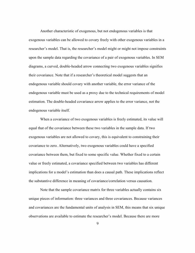
As a simple example to illustrate this idea, suppose that a researcher has a

hypothesis pertaining to three observed variables, x1, x2, and x3. The input covariance

matrix, S, would be formatted as in Figure 2.1. Each element along the main diagonal

represents the variance of an observed variable. Each off-diagonal element represents the

7

covariance of a pair of observed variables. Actual numerical estimates of these variances

and covariances would serve as the input data for analysis.

x1 x2 x3

x1

x2

x3

σσσσ x1

2

σσσσ x1x2σσσσ x2

2

σσσσ x1x3σσσσ x2x3

σσσσ x3

2

Figure 2.1. Format of a three variable covariance matrix.

Suppose the researcher’s hypothesis is that changes in variable x1 cause changes

in variable x2, and changes in x2 cause changes in x3, but changes in x1 do not directly

cause changes in x3. In other words, although x1 may or may not be related to x3 in terms

of the observed covariance of these two variables, any such relationship is hypothesized

to be fully accounted for by the mediating influence of x2. This is an example of a simple

path analysis, a type of SEM analysis that does not involve latent variables. This model is

diagrammed in Figure 2.2.

Figure 2.2. Path diagram for an example path analysis.

*x1

* *

x2 x3* *

8

Observed variables are represented by boxes. Asterisks represent parameters to be

estimated. The researcher’s hypotheses regarding the causal relationships among these

variables supposes the existence of five parameters: a causal path from x1 to x2, a causal

path from x2 to x3, the variance of x1, and two error variances; one for x2 and one for x3.

These parameters collectively comprise θθθθ, the vector of researcher-specified model

parameters. Notably, there is no parameter representing a direct connection between x1

and x3.

The directional nature of a causal path signifies that a change in the value of the

variable at the beginning of the arrow is thought to cause a change in the value of the

variable at the end of the arrow. That is, values of the variable at the end of the arrow are

thought to depend on values of the variable at the beginning of the arrow, but not vice-

versa. Variables with no incoming unidirectional arrows are known as exogenous

variables. Variables with at least one of these incoming causal paths are known as

endogenous variables. Variances of exogenous variables are usually estimated from the

sample data as model parameters, but may also be fixed at some specific value by the

researcher. Variances of endogenous variables may neither be estimated as model

parameters nor fixed. Instead, each endogenous variable has an associated error variance.

As shown in Figure 2.2, each error variance is essentially a separate exogenous variable,

complete with a causal path from this error variance to its associated endogenous

variable. Error variances are like other exogenous variables in that their specific

numerical value can be treated as a parameter to be estimated or fixed at some specific

value by the researcher.

9

Another characteristic of exogenous, but not endogenous variables is that

exogenous variables can be allowed to covary freely with other exogenous variables in a

researcher’s model. That is, the researcher’s model might or might not impose constraints

upon the sample data regarding the covariance of a pair of exogenous variables. In SEM

diagrams, a curved, double-headed arrow connecting two exogenous variables signifies

their covariance. Note that if a researcher’s theoretical model suggests that an

endogenous variable should covary with another variable, the error variance of the

endogenous variable must be used as a proxy due to the technical requirements of model

estimation. The double-headed covariance arrow applies to the error variance, not the

endogenous variable itself.

When a covariance of two exogenous variables is freely estimated, its value will

equal that of the covariance between these two variables in the sample data. If two

exogenous variables are not allowed to covary, this is equivalent to constraining their

covariance to zero. Alternatively, two exogenous variables could have a specified

covariance between them, but fixed to some specific value. Whether fixed to a certain

value or freely estimated, a covariance specified between two variables has different

implications for a model’s estimation than does a causal path. These implications reflect

the substantive difference in meaning of covariance/correlation versus causation.

Note that the sample covariance matrix for three variables actually contains six

unique pieces of information: three variances and three covariances. Because variances

and covariances are the fundamental units of analysis in SEM, this means that six unique

observations are available to estimate the researcher’s model. Because there are more

10

observations than model parameters, the model is described as overidentified. This is a

desirable property of models, and it is a necessary property for a model to be both

testable and parsimonious.

The full set of variances and covariances in the sample data may themselves be

regarded as a model of sorts. This model is saturated, because there are as many

parameter estimates as observations (Bollen, 1989). In this case, the parameter estimates

are also variances and covariances, i.e. the exact estimates that form the sample of data in

the context of SEM. Because of this, the observations will be replicated perfectly. If

diagrammed according to the conventions thus far presented, this model would show

every observed variable connected to every other observed variable by a double-headed

arrow. Models such as this one, with as many parameter estimates as observations, are

also known as just identified models. Just identified models do not posit the existence of

some simplifying causal process that is responsible for the observed variances and

covariances, and thus offer no falsifiable model in the SEM sense.

In many ways, overidentification is the heart of SEM. In specifying a model that

is comprised of fewer parameters than the total number of variances and covariances in

the sample data, the researcher has proposed an idea about the data that may or may not

be tenable. The overidentified model is more parsimonious than the just identified model,

because it seeks to account for the values of the observations using fewer parameters than

the total number of variances and covariances.

Estimates of the numerical values of the parameters are sought that reproduce the

sample variances and covariances as closely as possible given the restrictions imposed by

11

the researcher’s model. The degree of fit between the sample variance-covariance matrix

and its model-implied counterpart are the basis for a statistical test of the researcher’s

model.

Bollen (1989) gives the basic equation that formally expresses the fundamental

hypothesis of most structural equation models:

∑ = ∑(θθθθ) (2.1)

This equation, known as the covariance structure hypothesis, asserts that the population

covariance matrix (∑) is equal to a covariance matrix implied by model parameters in the

vector θθθθ. This equation thus represents the null hypothesis that the researcher has

specified a correct model. As Bollen notes, a vast array of statistical techniques such as

multiple regression, CFA, canonical correlation, ANOVA, ANCOVA, panel data analysis

and many others may be expressed in terms of this hypothesis. It should be noted

however that not all of these techniques (e.g., multiple regression) involve overidentified

models.

The hypothesis illustrated by Equation 2.1 is tested using the sample variance-

covariance matrix, S, in place of ∑. Estimated model parameters are used to form ∑( ˆ θ θ θ θ ),

the model-implied covariance matrix. This matrix is used as a substitute for ∑(θθθθ). The

specific numerical values of the parameter estimates comprising the vector ˆ θ θ θ θ are

obtained via one of several iterative estimation procedures. Three estimation procedures

for use with continuous observed variables are maximum likelihood (ML), generalized

least squares (GLS), and asymptotically distribution free (ADF). Each of these estimation

12

procedures is used to find a set of parameter estimates that minimizes simultaneously

each discrepancy between an element of S and the corresponding element of ∑( ˆ θ θ θ θ ). To

the extent that the estimation method functioned effectively, the resulting elements of ˆ θ θ θ θ

are the estimated parameter values that result in the least possible discrepancy between S

and ∑( ˆ θ θ θ θ ) given the specific form of the model specified by the researcher.

Let p equal the number of observed variables in a model. The number of unique

pieces of information present in S may then be defined as

2

)1(*

+=

ppp (2.2)

Because there are three observed variables, p* = 6 in the path analysis example above.

Degrees of freedom, v, for a model are defined as

v = p* - q (2.3)

where q is the number of parameters being estimated. Because there are only five

parameters to estimate, the model is overidentified with one degree of freedom. This

value of v forms the basis for a chi-square test of the model’s fit. The specific value of the

chi-square statistic is produced by the particular estimation method that is employed.

The magnitude of the chi-square statistic is negatively related to the

correspondence between the observed covariance matrix and the model-implied matrix.

When a model is correctly specified and assumptions associated with the use of a

particular estimation method are correct, the covariance structure null hypothesis is

correct and the expected value of the chi-square statistic is equal to its degrees of

freedom. In practice, the correctness of a researcher-specified model is not known.

13

Therefore, given that the chosen estimation method is appropriate for the sample data,

values of the chi-square statistic that are improbably large given their associated degrees

of freedom can be interpreted as evidence that the null hypothesis of a correct model is

not tenable.

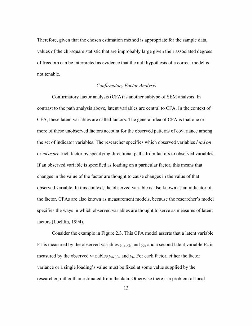
Confirmatory Factor Analysis

Confirmatory factor analysis (CFA) is another subtype of SEM analysis. In

contrast to the path analysis above, latent variables are central to CFA. In the context of

CFA, these latent variables are called factors. The general idea of CFA is that one or

more of these unobserved factors account for the observed patterns of covariance among

the set of indicator variables. The researcher specifies which observed variables load on

or measure each factor by specifying directional paths from factors to observed variables.

If an observed variable is specified as loading on a particular factor, this means that

changes in the value of the factor are thought to cause changes in the value of that

observed variable. In this context, the observed variable is also known as an indicator of

the factor. CFAs are also known as measurement models, because the researcher’s model

specifies the ways in which observed variables are thought to serve as measures of latent

factors (Loehlin, 1994).

Consider the example in Figure 2.3. This CFA model asserts that a latent variable

F1 is measured by the observed variables y1, y2, and y3, and a second latent variable F2 is

measured by the observed variables y4, y5, and y6. For each factor, either the factor

variance or a single loading’s value must be fixed at some value supplied by the

researcher, rather than estimated from the data. Otherwise there is a problem of local

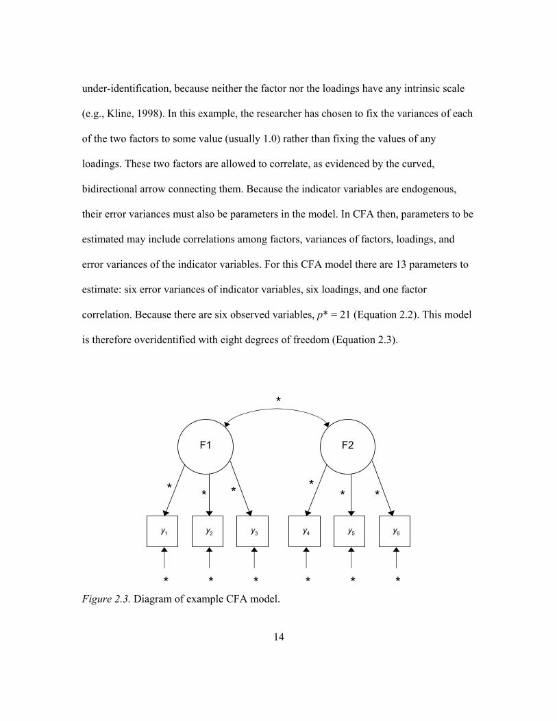
14

under-identification, because neither the factor nor the loadings have any intrinsic scale

(e.g., Kline, 1998). In this example, the researcher has chosen to fix the variances of each

of the two factors to some value (usually 1.0) rather than fixing the values of any

loadings. These two factors are allowed to correlate, as evidenced by the curved,

bidirectional arrow connecting them. Because the indicator variables are endogenous,

their error variances must also be parameters in the model. In CFA then, parameters to be

estimated may include correlations among factors, variances of factors, loadings, and

error variances of the indicator variables. For this CFA model there are 13 parameters to

estimate: six error variances of indicator variables, six loadings, and one factor

correlation. Because there are six observed variables, p* = 21 (Equation 2.2). This model

is therefore overidentified with eight degrees of freedom (Equation 2.3).

Figure 2.3. Diagram of example CFA model.

F1

y2

F2

** *

***

*

y3

y4

y1

y5

y6

* * ****

15

As with the example path analysis, the fact that v is greater than zero means that

the model is overidentified, and is thus placing restrictions on the pattern of

intercorrelation among the observed variables. For example, note that this model

accounts for observed covariances among variables y1, y2, and y3 via their loadings on the

factor F1. That is, this model asserts that any observed covariance between y1, y2, and y3

can be attributed to the latent variable F1’s causal effects on each of these variables. The

sample covariance of y1 with y3, for instance, will be reproduced by this model to the

extent that the estimates of these two variables’ loadings on F1 are jointly consistent with

σ13. Note, however, that the reproduction of σ13 is not the only criterion for the selection

of estimates of these loadings. For example, the loading of y1 on F1 is also involved in

the model’s reproduction of σ14, the covariance of y1 with y4. These are only two of the

competing demands placed on this loading by this particular model specification. An

optimal numerical estimate of this loading represents a compromise among these

demands. Competing demands of this nature are germane to the concept of overidentified

models. If the assumptions of the employed estimation method have been met, a

researcher-specified model is less tenable to the extent that parameter estimates that

closely reproduce the sample covariances cannot be found.

Estimation Methods for Continuous Data

Normal Theory Estimators

When observed variables are continuous, maximum likelihood (ML) and normal

theory generalized least squares (NTGLS) are common estimation methods, although ML

seems to have gained wider acceptance and is the default estimator in many SEM

16

software applications. These are known as normal theory (NT) estimators due to their

incorporation of the assumption of multivariate normality of the observed variables (e.g.,

Finney & DiStefano, 2006; West, Finch & Curran, 1995). Bollen (1989) gives the

following formula for the ML fit function:

FML = log|∑(θθθθ)| + tr(S∑-1

(θθθθ)) – log|S| - (p + q) (2.4)

where “tr” denotes the trace operator, which signifies the summation of the elements

along the main diagonal of the matrix to which it applies. The following is the generic

generalized least squares fit function:

FGLS = (1/2) tr({[S - ∑(θθθθ)]W-1

}2) (2.5)

Bollen (1989) notes that a variety of choices are available for W, the GLS weight

matrix, and that when S is used for W the version of GLS estimation found in LISREL

and EQS is reproduced:

FNTGLS = (1/2) tr{[I - ∑(θθθθ)]S-1

}2 (2.6)

This specific GLS estimator is referred to here as the normal theory generalized least

squares estimator, NTGLS, which is the particular version of the GLS estimator

discussed in West et al. (1995) and Muthén (1993).

When model specification is correct, the quantities FML(N – 1) and FNTGLS(N – 1)

are each asymptotically chi-square-distributed with degrees of freedom equal to the

number of observed variables minus the number of free parameters in the model (Bollen,

1989). With adequate sample size, the minimum of either the ML or the NTGLS fit

function may be therefore be multiplied by (N - 1) and evaluated as a chi-square statistic

17

with v degrees of freedom (see Equation 2.3). This chi-square statistic tests the null

hypothesis of correct model specification that is illustrated in Equation 2.1. Given that

assumptions for the use of this statistic are met, improbably large values given the

degrees of freedom signal a corresponding improbability that the specified model is

correct in the population from which the sample data were drawn. However, it must be

noted that small values of this statistic do not necessarily imply that a model is correctly

specified. It is possible for two or more models to make radically different claims about

cause and effect among the variables, yet exhibit identical fit to the data. Standard SEM

texts such as Bollen (1989) and Kline (1998) discuss this problem of equivalent models.

Bollen (1989) further notes that the ML fitting function is actually a special case

of the GLS fitting function where ∑( ˆ θ ), the model-implied covariance matrix as updated

at each iteration, is used as W. Similarly, Finney and DiStefano (2006) note that both the

ML fit function and the NTGLS fit function may be expressed as in Equation 2.6 above,

with the stipulation that NTGLS uses S as the weight matrix whereas ML uses ∑( ˆ θ θ θ θ ).

Finney and DiStefano cite Olsson, Troye, and Howell (1999) in noting that model

misspecification induces a critical performance difference in these two estimation

methods because of this difference in the weight matrix employed. When a model is

correctly specified, the ML weight matrix will tend to equal S at the last iteration,

resulting in equivalent results across these two methods. But given misspecification,

NTGLS exhibits biased chi-square statistics and parameter estimates due to its static

weight matrix. This is perhaps why ML has become the most common default estimator

in SEM software for models where observed variables are continuous.

18

Inspection of Equations 2.4 and 2.6 shows that both FML and FNTGLS are functions

of ∑(θθθθ), the model implied covariance matrix. The model implied covariance matrix,

∑(θθθθ), is a function of both the parameter estimates (the elements of θθθθ; paths, loadings,

and variances of exogenous variables including error variances) and the model that has

been specified. Basic SEM sources such as Bollen (1989) and Kline (1998) discuss the

path tracing rules that govern how the model implied covariance matrix is calculated for a

given researcher-specified model and a particular set of parameter estimates θθθθ.

What has yet to be explained is how structural equation modeling software

packages actually make use of fit functions such as FML and FNTGLS in order to arrive a

particular set of optimal model parameter estimates θθθθ. Most of the common SEM fit

functions including FML and FNTGLS achieve smaller values as the model implied

covariance matrix becomes more similar to the sample covariance matrix. For ML and

NTGLS estimation, this can be confirmed via an examination of Equations 2.4 and 2.6.

The software employs numerical techniques to simultaneously search for specific values

of each element of θθθθ that, as a set, minimize the value of the fit function. The search for

these elements usually must proceed iteratively, with the value of the fit function being

successively recalculated after small changes are made to the parameter estimates. When

the search algorithm is no longer able to effect meaningful decreases in the fit function,

the algorithm stops. The set of parameter estimates at this final iteration then serves as the

set of parameter estimates for the model given the sample data and the particular

estimation method. Bollen (1989) covers this process in more detail, including an

example of the numerical methods behind ML estimation.

19

Both ML and NTGLS make the same assumptions, and both possess the same

desirable properties when these assumptions are met (Bollen, 1989; Finney & DiStefano,

2006; Kline, 1998; West, Curran & Finch, 1995). These estimation methods assume

independence of observations, a sufficiently large sample size, correct model

specification, and continuous, multivariate normally distributed data. Bollen explains

more about the assumption of multivariate normality. Though the derivation of ML

estimation presupposes the multivariate normality of all observed variables, a less

restrictive condition is required for both ML and NTGLS to retain their desirable

properties. In practice, the assumption of multivariate normality applies only to the

endogenous observed variables conditional upon the exogenous observed variables. That

is, the multivariate normality of the endogenous variables must be tenable across the

multivariate distribution of the exogenous variables. Therefore, exogenous dummy

variables or interaction terms are not necessarily a problem for the normal theory

estimators. When these assumptions are met, ML and NTGLS provide asymptotically

unbiased, asymptotically normally distributed, asymptotically efficient, consistent

parameter estimates, as well as valid standard errors for these parameter estimates.

Unfortunately, the assumption of multivariate normality is likely to be incorrect in

practice. For example, Micceri (1989) analyzed several hundred real data sets from the

behavioral sciences and found that few variables were normally distributed at the

univariate level. Given that univariate normality of each variable in a set of variables is a

necessary but not sufficient condition for the multivariate normality of the set,

multivariate normality seems unlikely to occur in practice.

20

Perhaps in acknowledgement of this reality, the robustness of the normal theory

estimators to violations of this assumption has received considerable empirical attention

(e.g., Chou & Bentler, 1995; Chou, Bentler, & Satorra, 1991; Curran, West, & Finch,

1994; Finch, Curran, & West, 1994; Finch, West, & MacKinnon, 1997; Hoogland &

Boomsma, 1998; Hu, Bentler, & Kano, 1992). In general, parameter estimates provided

by the NT estimators retain their unbiasedness in the face of violations of this

assumption, though these estimates are likely no longer efficient (Bollen, 1989).

Unfortunately however, chi-square values for the test of model fit tend to become inflated

as observed variables depart from normality, especially if positive kurtosis is involved.

This inflation means that a correct model is more likely to be erroneously rejected as

nonnormality increases. The standard errors provided by the NT estimators tend to

become deflated with increasing nonnormality, with positive kurtosis again being an

especially aggravating factor (Finney & DiStefano, 2006).

The degree of nonnormality that should contraindicate the use of NT estimation is

undoubtedly a subjective issue dependent on one’s interpretation of existing literature in

the context of a given application. In reviewing relevant research, Finney and DiStefano

(2006) offer rough guidelines of 2 and 7 as maximum acceptable values for univariate

skewness and kurtosis, respectively, and a maximum acceptable value of 3 for Mardia’s

normalized multivariate kurtosis statistic. Somewhat more liberally, Kline (1998) arrived

at rough guidelines of 3 and 10 as values of univariate skewness and kurtosis that should

warn of problems for NT estimation.

21

The Asymptotically Distribution Free Estimator

Browne (1982, 1984) developed an estimator that did not require the burdensome

assumption of multivariate normality. Using a weight matrix calculated in part with

fourth order moments of the observed data, Browne’s estimator provides asymptotically

efficient parameter estimates as well as correct standard errors and model test statistics.

This estimator has been variously referred to as asymptotically distribution free (ADF),

full weighted least squares, and arbitrary generalized least squares (Bollen, 1989; Flora

& Curran, 2004; Finney & DiStefano, 2006; West, Curran & Finch, 1995). The ADF

estimator takes the following form:

FADF = s − σσσσ( ˆ θ θ θ θ )[ ]′W−1s − σσσσ( ˆ θ θ θ θ )[ ] (2.7)

Here s is a vector containing all of the non-redundant elements of the sample variance-

covariance matrix, and is thus of length p* (see Equation 2.2). σσσσ( ˆ θ θ θ θ ) is the model-implied

analog to s. As with the estimators previously discussed, an iterative search algorithm

arrives at parameter estimates (i.e., elements of ˆ θ ) that minimize the value of FADF.

Whereas the weight matrices in ML and NTGLS estimation are p × p in size, the

ADF weight matrix is p* × p*. This is because the ADF weight matrix is actually an

estimated variance-covariance matrix of the sample variances and covariances

themselves. The phrase asymptotic covariance matrix is often used to denote weight

matrices of this type, in which each element is an estimate of the asymptotic covariance

between a pair of covariance estimates, where each of these covariance estimates pertains

to a pair of observed variables (e.g., Bollen, 1989; Flora & Curran, 2004; Finney &

22

DiStefano, 2006; Muthén, 1984; West, Curran & Finch, 1995). Bollen illustrates the

calculation of the asymptotic covariance of two covariance estimates, sij and sgh, where sij

is the estimated covariance of variable Zi with variable Zj, and sgh is the estimated

covariance of variable Zg with variable Zh:

ACOV(sij,sgh ) = N

−1(sijgh

* − sij

*sgh

* ) (2.8)

where

))()(()(1

1

*hhtggtjjt

N

t

iitijgh ZZZZZZZZN

s −−−−= ∑=

(2.9)

)()(1

1

*jjt

N

t

iitij ZZZZN

s −−= ∑=

(2.10)

∑=

−−=N

t

hhtggtgh ZZZZN

s1

* ))((1

(2.11)

for N observations. The asterisks signify that N instead of (N – 1) is used for these

estimates. It is sijgh

* specifically that is the “fourth order moment around the mean”

(Bollen, 1989, p. 426).

The ADF estimator requires only that observed variables be continuous with finite

eighth-order moments. Given these conditions, parameter estimates produced by the ADF

estimator are asymptotically unbiased, consistent, and efficient, standard errors are

asymptotically correct, and the test of model fit provided by (N - 1)FADF is asymptotically

distributed as a chi-square statistic (Bollen, 1989; Browne, 1982, 1984; Finney &

DiStefano, 2006; West, Curran & Finch, 1995). In principle, the ADF estimator is

23

therefore a powerful, theoretically sound, almost all-encompassing solution to problems

posed by nonnormal continuous data.

It is the special form of the ADF weight matrix that gives this estimation method

its desirable properties. But this weight matrix is also the source of the shortcomings of

ADF. Because the weight matrix is of dimensions p* × p*, it increases in size

exponentially as the number of observed variables increases. For example, whereas there

are 784 elements in W when there are seven observed variables, there are 11,025

elements when there are 14 observed variables. Because W must be inverted,

computational burden is often cited as one practical problem of ADF estimation.

Although the problem of computational intensity might be less relevant with computers

becoming ever faster, there is a still more serious problem related to the size of W. Very

large sample sizes seem to be required to achieve stable estimates of all of its many

elements. With smaller sample sizes and more observed variables, the large W matrix is

increasingly likely to be nonpositive definite and therefore not invertible (Bentler,

1989,1995; Bollen, 1989; Finney & DiStefano, 2006; West, Finch, &, Curran, 1995). For

this reason Jöreskog and Sörbom (1996) recommend 1.5p(p + 1) as a minimum sample

size when using ADF. Finney and DiStefano (2006) note that considerably larger sample

sizes than this are often required in practice for ADF estimation to converge to a valid

solution. As will be discussed below, very large samples are usually required to achieve

acceptable performance of parameter standard error estimates and tests of model fit. The

desirable asymptotic properties of the ADF estimator are rarely realized in practice.

24

Even given that ADF estimation has converged on a valid solution, the inherent

problem of reliable estimation of the elements of W for realistically sized models at

realistic sample sizes manifests itself in the form of positive biases of chi-square and

negative biases of both parameter estimates and estimated standard errors (Finney &

DiStefano, 2006; West, Finch, & Curran, 1995). In their study of the performance of chi-

square statistics in the context of an oblique three-factor CFA model with five indicators

per factor, Hu, Bentler, and Kano (1992) found that the ADF chi-square statistic

performed “spectacularly badly” (p. 351) except when N was very large. Even at N =

5000, which was the largest sample size in the study, the ADF chi-square statistic

resulted in rejecting a correctly specified model roughly twice as often as expected.

Curran, West, and Finch (1996) examined the performance of chi-square statistics

produced by various estimation methods for models with three oblique factors and three

indicators per factor with some cross-loadings. They found that for correctly specified

models with both normal and nonnormal data, ADF tended to produce acceptable chi-

square statistics only when N equaled 1000. The second largest sample size in their study

was N = 500. Other studies have suggested that similarly large sample sizes are required

for ADF to provide acceptably accurate parameter estimates and standard errors (Chou &

Bentler, 1995; Chou, Bentler, & Satorra, 1991; Finch, West, & MacKinnon, 1998;

Hoogland & Boomsma, 1998; Yuan & Bentler, 1997).

In general, ADF estimation is unlikely to be of practical value to applied

researchers unless an extremely large sample size is available. However, ADF estimation

does hold a very special place in the world of SEM because of its theoretical soundness

25

and asymptotic correctness. Despite its practical problems, it is in principle a kind of

brute force, fully accommodating, correct solution to problems posed by nonnormal

continuous observed variables. Unfortunately, very large sample sizes are required to

realize these desirable asymptotic properties.

Satorra-Bentler Scaling

Given the inflated chi-square statistics and deflated standard errors associated

with the use of NT estimators with nonnormal continuous data, Satorra and Bentler

(1994) developed a corrective scaling procedure that can be applied with NT estimation

methods. This scaling procedure reduces chi-square values and enlarges standard errors

according to the degree of nonnormality of the observed variables. Whereas the positive

bias induced by nonnormality often renders NT chi-square values uninterpretable, the

Satorra-Bentler (S-B) scaled chi-square values are designed to again follow the expected

chi-square distribution given the null hypothesis of correct model fit. The corrected chi-

square value is given by

χS−B

2 = k-1χNT

2 , (2.12)

where χNT

2 is the value of the chi-square statistic resulting from either ML or NTGLS

estimation and k is a constant. Equation 2.12 shows that as k increases in value, χS−B

2

decreases. The value of k is related to the amount of multivariate kurtosis present in the

data. If no kurtosis is present, k = 1 and χS−B

2 = χNT

2 . More kurtosis results in higher

values of k, and thus lower values of χS−B

2 . While S-B scaling modifies chi-square

estimates downward if at all, it simultaneously scales estimated standard errors upward in

26

an analogous fashion, again in accordance with the level of multivariate kurtosis present

in the data. The calculation of k is technically complex, and the interested reader is

referred to Satorra (1990) and Satorra and Bentler (1994) for details. It should be

explicitly stated that Satorra-Bentler scaling does not involve any adjustment to the actual

parameter estimates resulting from NT estimation.

Simulation studies have shown S-B scaled chi-square statistics outperform their

NT counterparts given correctly specified models and nonnormal data (Chou & Bentler,

1995; Chou, Bentler, & Satorra, 1991; Curran, West, & Finch, 1996; Hu, Bentler, &

Kano, 1992; Yu & Muthén, 2002). Furthermore, the positive chi-square bias of ML

estimation with nonnormal data that was observed in many conditions of these studies

bolsters the contention that this method is clearly inadequate for many realistic

circumstances involving nonnormal data. Though the S-B scaling of the chi-square

generally failed to completely eliminate positive bias in the NT chi-square values across

all conditions, these studies generally suggest that S-B scaling is a viable method for

applied researchers. Similarly, S-B corrected chi-square statistics have been shown to be

clearly superior to corresponding ADF chi-square values at small to medium sample

sizes, and to retain a small margin of superiority even at N = 1000 (Curran, West, &

Finch) and N = 5000 (Hu, Bentler, & Kano). S-B scaled standard errors likewise show

similar improvement over their ML and ADF counterparts (Chou & Bentler; Chou,

Bentler, & Satorra). In general, the S-B scaling procedure performs well enough to be a

serviceable solution to the problem of nonnormal observed variables in many situations

where ADF and ML are inadequate.

27

Maximum Likelihood, Satorra-Bentler Scaling and Asymptotically Distribution Free

Estimation with Misspecified Models

Interestingly, Curran, West, and Finch (1996) also included two conditions of

model misspecification in their study of bias in chi-square statistics. Though one

challenge of this approach was the determination of expected values for the chi-square

estimates of each estimation method given the particular model misspecification, these

expected values are themselves of theoretical interest. Curran et al. elected to approach

this issue by considering bias as occurring as a result of finite sample size. The method

they used to calculate expected values of the ADF and S-B scaled chi-square for purposes

of determining bias will illustrate this point. Curran et al. generated three very large (N =

60,000) simulation data sets according to the population model used throughout their

study. While each of these data sets corresponded to this population model, each data set

differed in the distributions of the observed variables. Each simulated data set’s observed

distributions matched one of the three conditions of observed variable distribution that

was used in the study: normal, with skewness and kurtosis of 0 for each indicator;

moderately nonnormal, with skewness = 2 and kurtosis = 7 for each indicator; and

severely nonnormal, with skewness = 3 and kurtosis = 21. Curran et al. then fitted each of

the two misspecified models in their study to each these data sets using ADF estimation

and S-B scaling separately, for a total of 12 separate model estimations. They then

extracted the minimized fit function from the resulting chi-square estimates for each of

these 12 large sample estimations (see, e.g., Equation 2.7 for the case of ADF

estimation), and rescaled them according to each of the sample sizes of interest in their

28

study (N = 100, 200, 500, and 1000). The model degrees of freedom were added to each

of these values in order to obtain large sample empirical estimates of expected chi-square

values for each specific combination of sample size, misspecified model, estimation

method, and distribution of observed variables. A similar procedure (Satorra & Saris,

1985) was used to calculate the expected values for ML estimation. Curran et al. then

used these estimated expected values to determine biases in chi-square for each of the

conditions involving a model misspecification. For this reason, bias in this context refers

only to bias resulting from small sample sizes.

As Curran, West, and Finch (1996) discuss, the expected values of these chi-

square statistics for each estimation method across conditions are interesting in their own

right. Because the degrees of freedom are the same across estimation methods for a

particular model misspecification, greater expected values of chi-square suggest that an

estimation method is more sensitive to model misspecification given the particular

observed variable distribution under consideration, apart from any bias associated with

decreasing N. The expected values of the ML chi-square and S-B scaled ML chi-square

were approximately equal for the misspecified models when indicator variables were

normally distributed. This was expected, given that S-B scaling is designed to correct for

nonnormality of the observed variables. In the absence of nonnormality, values of the S-

B scaled ML chi-squares should be approximately equal to their unscaled ML

counterparts. The expected values of the ADF chi-square were clearly lower than those of

the other two methods across conditions. As nonnormality increased, the expected values

of both the ADF chi-square and the S-B scaled chi-square decreased, whereas the

29

expected value of the ML chi-square remained the same. Curran et al. note that this

implies a relative lack of power of ADF and S-B scaling to detect model

misspecifications given nonnormally distributed variables.

Smaller sample size was associated with greater positive bias for all estimators

across all distributional characteristics of observed variables. However, ADF statistics

were especially notable for their substantial positive biases at small sample sizes, even in

the case of normally distributed observed variables. Both the ML chi-square and S-B

scaled ML chi-square showed little bias relative to their expected values given normality

of the observed variables. Though bias was worse at smaller sample sizes, it was small in

magnitude. Given normal variables, the ADF estimator exhibited substantial positive bias

at the two smaller sample sizes (N = 100 and 200), but little at N = 500 or 1000. All

methods generally showed increasing positive bias with increasing nonnormality. The S-

B scaled chi-square showed the least of this bias, although it was notable. Plain ML

showed more of this bias, and ADF showed large positive biases due to nonnormality,

especially at smaller sample sizes.

In discussing the decreasing expected values of the ADF and S-B scaled statistics

with increasing nonnormality, Curran, West, and Finch (1996) consider the idea of

signal-to-noise ratio. In this context, a model misspecification is the signal to be detected.

Because the ADF and S-B methods explicitly recognize and account for nonnormality in

the observed variables, their expected chi square values reflect the burden of detecting the

signal of misspecification amidst the noise of nonnormal distributions, which is of course

greater than the noise of normal distributions. Stated in a somewhat different way, both

30

ADF and S-B scaling utilize a proportion of the total information contained in any sample

of data to estimate distributional characteristics of these data. Relative to NT estimators,

the ADF and S-B methods necessarily have less information remaining for purposes of

evaluating the plausibility of a particular model specification. Because they simply

assume multivariate normality, NT estimators are not similarly burdened. This

explanation similarly explains the greater positive bias shown by the NT estimators given

a correctly specified model and nonnormal data. Because NT estimation methods are

incapable of disentangling nonnormality from misspecification, bias in favor detecting

the “signal” of misspecification is observed.

Estimation Methods for Ordered Categorical Data

As Bollen (1989) points out, limitations of measurement instruments technically

result in ordered categorical measurement even for variables that are typically thought of

as continuous. For example, even the most precise electronic scale for measuring weight

must nevertheless have some limit to the decimal places of its output, although the

variable weight itself is a perfectly continuous variable. The minimum number of unique

values that are required to designate an observed variable as continuous as opposed to

ordinal seems to be a subjective matter. For example, LISREL automatically treats

observed variables with 15 or fewer categories as ordered categorical variables unless this

default is overridden (Jöreskog & Sörbom, 1996). Five to nine categories seems to be a

recommended minimum number in many contexts.

The ML, GLS, and ADF estimation algorithms are appropriate when observed

endogenous variables are continuous. But in many instances researchers make use of

31

ordered categorical variables in their analyses. For example, annual income could be

measured with responses such as less than $20,000, $20,001 to $40,000, $40,001 to

$60,000, more than $60,000, or some other group of categories that together provide less

information than a specific dollar amount for each respondent. In this case, income itself

is of course a continuous variable. But it is not uncommon that continuous variables such

as income in dollars are only available to applied researchers in discrete, ordered

categories as above.

Likert responses to questionnaire items are one of the most commonly cited

examples of ordered categorical variables. Research participants might be asked to

respond to a series of questions using a scale such that Strongly Agree = 1, Agree

Somewhat = 2, Disagree Somewhat = 3, and Disagree Strongly = 4. In principle, a

researcher could use only two categories (e.g., Agree = 0, Disagree = 1) or a much larger

number of categories. Thus the distribution of any particular observed variable of this

kind is in large part an artifact of the researcher’s decision regarding the number of

response alternatives for the Likert variable. Participants’ true levels of agreement or

disagreement with any particular statement would likely form a continuous distribution of

some type (Bollen, 1989; Finney & DiStefano, 2006; Muthén, 1984; West, Curran &

Finch, 1995). As with the annual income example above, the Likert question format is an

example of the artificial categorization of responses into a finite number of discrete,

ordered groups in order to facilitate measurement. In many instances, an ordered

categorical variable may be understood as the observed result of some measurement

32

process artificially grouping values of a continuous variable into a relatively small

number of discrete, ordered categories.

Modern approaches for statistical modeling with ordered categorical data consider

the distinction between the observed ordered categorical variable, y, and the hypothetical

underlying continuous variable that was coarsely categorized in the process of

measurement, y*. This approach is known as the latent response variable formulation,

and the y* variable is often referred to as a latent response variable (Finney & DiStefano,

2006; Muthén & Muthén, 2005).

There are at least three reasons for acknowledging the distinction between y and

y* when performing covariance structure analysis on ordered categorical data (Bollen,

1989; Finney & DiStefano, 2006; Muthén, 1984). First, while the distributions of the

ordered categorical y variables are always fundamentally nonnormal due to the non-

continuous nature of categorical data, these distributions are also likely to be nonnormal

as indexed by measures of skewness and kurtosis. When more than one y variable is

involved, multivariate distributions are also likely to be substantially nonnormal. Bollen

points out that although one could use ADF for estimation of the model in this case,

heteroscedastic errors can result from ordered categorical variables. That is, the variance

of the residuals of the y variables as predicted by the factors may differ across the y

variables. This violates an assumption of ADF estimation. Second, as stated by Finney

and DiStefano, “the standard linear measurement model specifies that a person’s score is

a function of the relation (b) between the variable (y*) and the factor (F) plus error (E):

33

y* = bF + E” (2006, p.309). But because y ≠ y*, it follows that y ≠ bF + E, and thus this

standard model is inappropriate for direct application to y (see also Bollen, 1989).

But according to Bollen (1989), a more severe consequence of treating ordered

categorical variables as though they are continuous is a violation of the covariance

structure hypothesis given in Equation 2.1. When observed variables are continuous, the

covariance structure hypothesis is usually formulated as in Equation 2.1. When observed

variables are ordinal however, we know that in most cases the specific form of the

ordinalization is arbitrary, and is of no intrinsic interest. Instead, we are interested in the

continuous variables that are assumed to have given rise to these observed ordinal

variables. Because we are interested in these latent y* variables, we now formulate the

covariance structure hypothesis as

∑* = ∑ (θθθθ) (2.13)

where ∑* is the population covariance matrix of the latent, continuous y* variables.

Because the covariance matrix of latent response variables is not equivalent to the

covariance matrix of the observed, ordered categorical variables, i.e. Σ* ≠ Σ, the

covariance structure hypothesis is not properly tested when ordinal data are directly

analyzed as though they were continuous.

The assertion that direct analysis of the observed ordered categorical variables

violates the covariance structure hypothesis presupposes that the covariance structure

hypothesis pertains to the latent response variables and not the ordered categorical

variables. That is, it is assumed that the covariance structure hypothesis is in fact

Equation 2.13 and not Equation 2.1. This formulation of the covariance structure

34

hypothesis seems to be universal among authors in this field (e.g., Bollen, 1989; Flora &

Curran, 2004; Finney & DiStefano, 2006; Jöreskog & Sörbom, 1996; Muthén, 1984;

West, Curran & Finch, 1995).

Simulation studies that have examined the effects of analyzing ordered categorical

data with estimators that are designed for continuous data have reflected this assumption

in their data generation procedures (e.g., Babakus, Ferguson, & Jöreskog, 1987; Dolan,

1994; Green, Akey, Fleming, Hershberger, & Marquis, 1997; Muthén & Kaplan, 1985;

Potthast, 1993). The population models that have been used in these studies, including

factor loadings, factor correlations, etc., typically were first defined in terms of a

covariance or correlation matrix of continuous, multivariate normal “observed” variables.

Population values (e.g., for factor loadings) that were to be used for purposes of

examining bias applied to the data generated at this stage. After sample data were

generated in this form, each value of a continuous variable was categorized according to

a set of thresholds in order to yield a value on a more coarse ordinal scale. The previously

observed continuous variables therefore became latent variables at this stage, with only

their observed ordinal counterparts available for analysis.

For example, scores for each simulated individual observation on each factor

indicator might have initially been randomly generated on a standard normal scale, i.e. M

= 0, SD = 1, according to an overall correlational structure consistent with a population

model of interest. Then, each value for the continuous indicator variables would be

transformed into a value on an ordinal scale according to the particular range in which the

value fell. For example, all generated values lower than z = -1.00 could be assigned a

35

value of 1, values between z = -1.00 and z = +1.00 could be assigned a value of 2, and all

values above z = 1.00 could be assigned a value of 3. This procedure would result in a

three-category ordinal symmetric factor indicator whose (now latent) parent continuous

distributions corresponded to the population model of interest. These z values serve as

thresholds that segment the originally continuous simulated data into ordered categorical

data. The thresholds, and thus the distributional properties of the observed variables, can

be arbitrarily varied just as any other design factor in a simulation study.

Normal Theory Estimators with Ordered Categorical Data

Problems associated with treating ordered categorical data as though they were

continuous result from the imperfection of the y variables as measures of the y* variables,

and thus of ∑ as a measure of ∑*. Intuitively then, categorical transformations of

previously continuous variables should cause greater problems to the extent that they

obscure the distributional shapes of the original variables. To the extent that the

distributional shape of the original variable has been obscured, more information has

been lost. For this reason, segmenting a continuous variable into an ordinal variable with

relatively few categories is likely to be a more corrupting transformation of the original

distribution than when the resulting ordinal variable has more categories. This is because

relatively more observations that were previously distinct from one another are now

treated identically. Categorical variables with fewer categories should therefore be

associated with poorer recovery of model parameters, which are defined at the level of

the continuous, unobserved y* variables. Standard errors and tests of overall model fit

should be similarly compromised.

36

Research on the robustness of the Pearson correlation coefficient to the coarse

categorization of continuous variables supports this idea and foreshadows some of the

problems associated with the application of NT estimators to ordinal data in SEM.

Several studies have compared the Pearson correlations of pairs of continuous variables

with the Pearson correlation of these variables after one or both have been transformed

into ordered categorical variables via the application of thresholds as described above.

Not surprisingly, correlations tend to be lower after continuous variables are segmented

into discrete categories, with fewer categories resulting in lower correlations. Segmenting

variables so that they have opposite skew particularly attenuates correlations (Bollen,

1989; Bollen & Barb, 1981; Olsson, Drasgow, & Dorans, 1982).

Not surprisingly then, simulation studies have in fact demonstrated that the

theoretical inappropriateness of using NT estimators on ordered categorical observed

variables is associated with real consequences in the context of SEM. The first

consequence is a tendency for chi-square statistics to be positively biased. For example,

Dolan (1994) examined various estimators including ML as they performed at sample

sizes of 200, 300, and 400 for a single factor CFA model with eight indicators. The

originally continuous indicators had been transformed into ordinal variables with 2, 3, 5,

or 7 categories. The distributions of these transformed variables were either near-normal

(rectangular in the 2 category case) or mildly skewed. Chi-square statistics showed

unacceptably high positive bias when the indicators had been transformed to have fewer

than five categories, and when the five- and seven-category indicators were skewed. Chi-

square bias was positive but marginally acceptable in the five-category normally shaped

37

condition, and acceptable in the seven-category normally shaped condition. In a study of

one factor, 20 indicator CFA models, Green, Akey, Fleming, Hershberger, and Marquis

(1997) similarly found that transformations of continuous indicators that resulted in fewer

categories led to greater inflation of chi-square. Chi-square performance was acceptable

with six-category indicators, but four-category indicators tended to result in unacceptable

levels of inflation. There was no five-category condition. In general, increased

nonnormality of the transformed indicators also resulted in greater chi-square bias.

Muthén and Kaplan (1985) looked at the effects of segmenting continuous factor

indicators into five-category ordinal variables for a one-factor, four-indicator model at a

sample size of 1000 per replication. As with the previously discussed studies, the model

was correctly specified when estimated apart from the fact that the ordinalization of the

originally continuous indicators was ignored during model estimation. Both ML and

NTGLS were among the estimators they examined. In one condition, the indicators were

categorized so that they were approximately normally shaped. Four other conditions

represented various types of nonnormality. Based on the expected value of 2, i.e. the

model degrees of freedom, chi-square was overestimated for both ML and NTGLS across

all indicator distributions. Skewness and negative kurtosis both generally caused more

bias. Interestingly, a positive-kurtosis-only condition exhibited the least bias at roughly

+14%. Bias of roughly +30% was associated with the normally shaped indicators.

A study by Babakus, Ferguson, and Jöreskog (1987) was similar in that the same

single factor model as in Muthén and Kaplan (1985) was considered, and the originally

continuous indicators had been segmented into five-category ordinal variables. These

38

authors considered normally shaped indicators as well as four different conditions of

nonnormal indicators at sample sizes of 100 and 500. Maximum likelihood estimation

applied to the Pearson correlation matrix resulted in little chi-square bias for the normally

shaped ordinal indicators. But bias was unacceptably high in the nonnormal conditions,

and was greater with greater nonnormality. Bias was roughly +15% given U-shaped

indicators with negative kurtosis, and was greater than or equal to this value given

indicators that were skewed but not U-shaped, or were mixes of different shapes of

nonnormal indicators. Bias was worst in the condition in which the four indicators had

the most skew, equaling roughly +40%.

As expected, factor loadings are generally underestimated when categorical data

are treated as continuous and analyzed with NT estimators. Dolan (1994) found that

underestimation was at roughly 5% in both the normal and skewed five-category

conditions given ML estimation, substantially worse in the two- and three-category

conditions, and somewhat better in the seven-category conditions. The normal versus

nonnormal distinction did not appear to have a consistent effect on parameter estimates

given ML estimation. Babakus et al. (1987) found that categorization induced an

underestimation of the loadings of slightly less than 5% given normally shaped

categorical indicators. Increasing nonnormality caused more severe underestimation such

that underestimation was at slightly worse than 15% in the most skewed condition. The

bias estimates of Babakus et al. came from direct comparisons of analyses of the same

samples of data with and without the categorization.

39

Muthén and Kaplan’s (1985) study was slightly unusual in that they fixed a

loading to the known population value in order to identify the model, rather than fixing

the factor variance. Because of this, the attenuation of the covariances among the

indicators was not manifested in downwardly biased loadings as it was in Dolan (1994)

and Babakus et al. (1987). Instead, attenuation was manifested in the form of

downwardly biased factor variance estimates and upwardly biased indicator error

variance estimates. Factor variance estimates showed highly similar levels of downward

bias for both ML and NTGLS estimation. In the case of normally shaped categorical

indicators, this bias was roughly –7%. Bias was more severe when the indicator variables

were more nonnormal, reaching a maximum of roughly 27% negative bias for the highly

skewed conditions. For the symmetrical, kurtosis-only condition, negative bias was

approximately 26%. In general, the estimated error variances showed levels of positive

bias that were slightly greater than the negative bias observed in the factor variance

estimates.

There is an interesting inconsistency among these studies regarding the

performance of the standard error estimates that are provided by normal theory estimators

when these estimators are applied to coarsely categorized data. Both Babakus et al.

(1987) and Dolan (1994) found that, relative to the empirical standard deviations of the

parameter estimates, ML estimated standard errors were inflated. In Babakus’s findings,

estimated standard errors were roughly 33% inflated given normally shaped indicators.

Greater skew led to larger empirical standard deviations of parameter estimates, but

somewhat less overestimation of the SEs. The empirical standard deviations of the

40

parameter estimates were the largest in the most nonnormal condition, but the estimated

standard errors were equal to the empirical SDs.

Standard errors from ML estimation were similarly inflated in Dolan (1994).

Recall that Dolan included 2-, 3-, 5-, and 7-category indicator conditions that were either

approximately normal or asymmetric in shape, whereas Babakus et al. (1987) examined

5-category indicators across five separate indicator distribution conditions. Dolan found

that the estimated standard errors from ML estimation were largely a function of the

sample size, showing little sensitivity to the number of categories or the distribution of

the indicators. In contrast, the empirical standard deviations showed sensitivity both to

sample size and to the number of categories: greater sample size led to less variation, and

fewer categories led to more variation. The combination of these patterns led to greater

inflation of the ML-provided standard errors when there were more categories. Inflation

tended to be about 100% in the seven-category conditions, but about 20% in the two-

category conditions. With fewer categories, greater sample size was associated with

relatively less overestimation. Sample size had little effect on overestimation when the

number of categories was large. Normality versus asymmetry of the indicators had no

consistent effect on the empirical standard deviations, the estimated standard errors, or

the degree of overestimation.

Muthén and Kaplan’s (1985) finding regarding ML standard errors are in contrast

to those documented above. Recall that Muthén and Kaplan examined five-category

indicator variables across five different distributional shapes of these ordinal indicators.

When indicators were approximately normally shaped, ML and NTGLS standard errors

41

for the loadings and indicator error variances were approximately correct, and standard

errors for the factor variance estimates tended to show inflation relative to the empirical

standard deviations of these estimates. But interestingly, as nonnormality increased, the

NT estimators tended to provide negatively biased standard errors relative to the

empirical standard deviations of the estimates of loadings and variances. These findings

echoed those of an earlier study by Boomsma (1983), who also found that estimated

standard errors became too small as nonnormality increased when ML estimation was

applied to coarsely categorized data.

This discrepancy in the performance of the standard errors could perhaps be

explained by the type of input data used in each of the studies. Whereas Muthén and

Kaplan (1985) and Boomsma (1983) applied the normal theory estimators to the raw data

(i.e., the unstandardized covariance matrix of the ordinalized variables), Babakus et al.

(1987) and Dolan (1994) applied ML to the Pearson product-moment correlation matrix

of the ordinal observed variables. Though they did not report analyses of unstandardized

data, Babakus et al. seemed to acknowledge the possibility that standardization affects

standard error estimates: “…when the input data were standardized [emphasis added],

LISREL overestimated the standard errors relative to the empirical estimates” (p. 225).

The overestimation also occurred when the continuous data were analyzed via Pearson

product-moment correlations. Although incongruent, the results of these studies

nevertheless show that the standard errors provided by NT estimators are likely to be

inaccurate when these estimators are applied to coarsely categorized data. One cannot

have confidence in these standard errors, even given approximately normally distributed

42

five-category indicators. Any nonnormality of the indicators is likely to exacerbate the

problem, whether it is inflation or deflation of the estimated standard errors relative to

their empirical variability.

The results discussed above might be interpreted as suggesting that the problems

of using NT estimators with categorical data might not be prohibitive, provided that

indicators are approximately normally distributed and have perhaps five or more

categories. However, it is probably unlikely that categorical indicators will uniformly

assume approximately normal shapes (Micceri, 1989). Furthermore, it is important to

note that relatively simple models were used in these studies. In many applied instances,

models will be more complicated than those discussed above. It is wise to suspect that

more complicated models, especially in interaction with smaller sample sizes and

nonnormally shaped indicators, might exacerbate the performance problems associated

with the normal theory estimators when they are applied to ordered categorical data. Even

under the best conditions, standard errors might be of unpredictable quality. In general, it

is probably unwise for applied researchers to use NT estimators with categorical data.

Satorra-Bentler Correction with Ordered Categorical Data

Recall that the Satorra-Bentler scaling procedure applies a correction to the chi-

square statistic and standard errors in an attempt to accommodate violations of the NT

estimators’ assumption of multivariate normality. Though the S-B correction is intended

for use with continuous data, a limited amount of empirical research has examined its

performance with coarsely categorized variables. It is important to note that because the

43

S-B correction makes no adjustment to the parameter estimates, any bias induced by

categorization will remain for these estimates.

Green, Akey, Fleming, Hershberger, and Marquis (1997) examined the effect of

S-B scaling on chi-square estimates, and DiStefano (2002, 2003) considered both chi-

square estimates and standard errors. In general, the S-B correction did in fact usefully

reduce bias in both the SEs and the chi-square estimates to a degree that should not be

particularly surprising given the performance of S-B scaling with nonnormal continuous

data. The most interesting finding, however, occurred in Green et al.’s mixed-skew

conditions. In these conditions, some factor indicators had negative skew and some had

positive skew. Unscaled chi-square estimates provided by ML under these circumstances

were vastly more inflated due to categorization than in other conditions. But in these

mixed-skew conditions, the improvements of S-B scaled chi-square estimates over their

unscaled counterparts virtually disappeared. Mixed skew with coarsely categorized data

apparently is not only a particular challenge for ML estimation, but also defeats the

improvements normally offered by the S-B scaling procedure.

Polychoric Correlations

If the covariance structure hypothesis is specified with regard to the covariances

of y* and not y, the aforementioned empirical failures of direct application of ML

estimation to correlation and covariance matrices calculated directly from the ordinal

variables suggest the necessity of having a sample estimator of Σ*, the covariance matrix

of the y*. A matrix that serves as ˆ ∑ * is formed by estimating polychoric correlation

coefficients for each of the p(p - 1)/2 pairwise combinations of the y variables. A

44

polychoric correlation coefficient estimates the Pearson correlation that would result for a

pair of ordered categorical variables if these variables’ unobserved y* distributions were

available (Jöreskog & Sörbom, 1996; Olsson, 1979).

For polychoric, polyserial, tetrachoric and biserial correlations to be estimated, it

is necessary to make assumptions regarding the distributional shapes of any y* variables

involved. The distributional shape of any particular latent response variable can of course

never be observed. These y* distributions are hypothetical only, and the specific

distributional form used to represent any particular y* is highly arguable and essentially

arbitrary. The standard normal distribution is commonly assumed as a matter of

convenience (Muthén, 1983, 1984).

Sources such as Bollen (1989), Finney and DiStefano (2006), Flora and Curran

(2004), Muthén and Kaplan (1985), and Finch, West, and Curran (1995) review the

procedure whereby the link between y and y* is operationalized. Equation 9.101 from

Bollen is a typical example of this operationalization. This equation illustrates the

mapping of responses on the observed variable y1 with the associated latent response

variable y1*:

y1 =

1, if y1* ≤ a1

2, if a1 < y1* ≤ a2

M M

c −1, if ac−2 < y1* ≤ ac−1

c, if ac−1< y1 *

(2.14)

The observed variable y1 has c categories (e.g., c separate levels of agreement or

disagreement for a Likert questionnaire response). The latent response variable y1* is

45

arbitrarily scaled as a standard normal distribution. The ais are thresholds that link

regions of y1* with the discrete values of y1.

Equation 9.102 from Bollen (1989) demonstrates one method of estimating the

thresholds when the latent response variable is assumed to follow a standard normal

distribution:

ai = Φ−1 Nk

Nk=1

i

∑

, i =1,2,K,c −1 (2.15)

“where Φ–1

(.) represents the inverse of the standard normal distribution function, Nk is the

number of observations which fall in the kth category, and c is the total number of

categories for y” (p.440).

This intuitively appealing procedure essentially provides the estimated thresholds

(ais) as z-scores on the latent response variable. For example, suppose we have a Likert

item to which 1000 total people responded. Suppose 75 of these 1000 people endorsed

the lowest or leftmost response on this item, e.g. strongly disagree. Because 75/1000 =

7.5%, and because –1.44 is the z-score that demarcates the bottom 7.5% of the standard

normal distribution, -1.44 is the first threshold. If 200 of the 1000 respondents endorsed

the second lowest/leftmost category (e.g., disagree somewhat), then a total of (75 +

200)/1000 = 27.5% of the sample scored at or below the second category. The second

threshold would thus be estimated as -.60, the z-score that demarcates the bottom 27.5%

of the standard normal distribution.

To estimate a particular polychoric correlation, more information than the

estimated univariate thresholds must of course be involved. The statistical association of

46

the variables in their original ordered categorical state must be considered. A contingency

table for a pair of ordinal variables contains information about the mutual association of

these two variables. This is the only available empirical information about the correlation

of the latent variables. Consider the following example in which 1000 hypothetical

respondents have provided answers to two Likert items. Item A has three categories. Item

B has four categories. The numbers of individuals who endorsed each combination of

responses to these two variables are shown in Table 2.1.

Table 2.1

Joint Frequency Distribution of Two Hypothetical Likert Variables

Item B

Strongly Agree Agree Disagree Strongly Disagree

Item A Agree 20 29 122 98

Neutral 64 134 111 55

Disagree 145 188 22 12

This joint frequency distribution provides information about the correlation of the

original ordered categorical y variables. The cell counts of this frequency distribution and

the set of thresholds for each variable are used to form a likelihood function. This

likelihood function also incorporates Φ2, the bivariate normal distribution function given

a particular Pearson correlation value, ρ. ρ is treated as an unknown along which the

function varies, and the likelihood function is maximized using maximum likelihood

estimation. The value of ρ that maximizes the likelihood of the function then serves as

47

the estimate of the polychoric correlation of variables A and B. Alternatively, the

thresholds for each of the two variables may also be treated as unknowns along which the

likelihood function may vary. The likelihood function is then maximized with respect to

the thresholds and ρ simultaneously. This procedure is more computationally intensive

however, and does not seem to be notably superior to treating the thresholds as fixed

values in the likelihood function (Bollen, 1989; Olsson, 1979).

Polychoric Correlations with Normal Theory Estimators

Given the theoretical appropriateness of the polychoric correlation as an estimate

of the correlation between two coarsely categorized variables, the use of a normal theory

estimator with a matrix of these correlations might seem like a very reasonable approach

to the problem of conducting SEM analyses with ordinal data. In fact, applying a normal

theory estimator to a matrix of polychoric correlations has been shown to be quite

effective in recovering the factor loadings for the latent y* variables that have been

coarsely categorized to form observed indicators. Unfortunately, simulation studies have

been unanimous in finding two serious problems with this approach. Estimated standard

errors have been found to be unpredictable and often quite biased, and chi-square values

tend to be wildly inflated.

Recall that Babakus, Ferguson, and Jöreskog (1987) studied a one factor CFA

model at sample sizes of 100 and 500 with four continuous indicators that had each been

coarsely categorized into indicators with five categories. Normally shaped categorical

indicator scores as well as four conditions of nonnormal categorical indicators were

considered. Among other estimation strategies, Babakus et al. applied the ML estimator

48

to a matrix of polychoric correlations calculated from the ordinal data. As is the case with

most CFA studies involving ordinal variables, interest was in the recovery of the

parameters for the continuous population factor model for the y* variables that were used

to generate the observed ordinal variables. Calculation of the polychoric correlations of

course represented an attempt to estimate the correlations among the original y*

variables. When ML estimation was applied to the polychoric matrix, parameter

estimates closely corresponded to those of the population model for the continuous y*

variables. There was essentially no bias in the estimated loadings, even for the most

nonnormal categorical indicators. Greater departures from normality did cause somewhat

greater variability in the loading estimates, however. Standard errors were somewhat

inflated relative to the empirical standard deviations of the estimates when the indicators

were normally shaped. But in some of the more extremely nonnormal conditions, the

standard errors actually showed considerable negative bias. Intermediate indicator

nonnormality produced approximately accurate standard errors.

For chi-square estimates, 50% inflation was the least amount observed and

occurred with the normally shaped indicators. Greater nonnormality resulted in greater

positive bias, reaching roughly 300% chi-square inflation in the most nonnormal case.

Additionally, the p-values associated with these chi-square estimates were not uniformly

distributed. It is worth noting that Babakus, Ferguson, and Jöreskog (1987) also

examined the performance of ML estimation with Pearson product-moment correlations

(as previously discussed), as well as Kendall’s tau-b and Spearman’s rho correlations and

found these approaches to also be generally inadequate.

49

Rigdon and Ferguson (1991) examined a variety of estimators including ML and

NTGLS as they performed with polychoric correlations for the estimation of two factor

CFA models with four indicators per factor. As in Babakus, Ferguson, and Jöreskog

(1987), the population factor model was generated with continuous indicators which were

then segmented into indicators with five categories. Again, interest was in recovering

parameters from the population factor models for the continuous indicators. Conditions

were included in which the categorical indicators had the same distributional

characteristics as in Babakus et al., but at sample sizes of 100, 300, and 500. Rigdon and

Ferguson did not present specific results for each cell of the study, but instead

summarized across design factors. Nevertheless, it was clear that chi-square values were

seriously inflated when either NTGLS or ML estimation was applied to a polychoric

correlation matrix. As with Babakus et al., parameter estimates were unbiased. In general,

standard errors were unacceptably biased. The specific type and amount of bias depended

on the shape of the distribution, but was not presented in detail.

Recall that Dolan (1994) studied one factor, eight indicator CFA models at

sample sizes of 200, 300, and 400 with indicator variables that had been categorized to

have 2, 3, 5, or 7 categories. The resulting categorical indicators were either roughly

normally shaped (rectangular in the 2-category condition) or somewhat skewed. Among

other estimation strategies, and like Babakus, Ferguson, and Jöreskog (1987) and Rigdon

and Ferguson (1991), Dolan included ML estimation applied to a polychoric correlation

matrix formed from the categorical indicators. This technique again yielded estimates of

the factor loadings for the population y* model that were extremely accurate, and far

50

more accurate than the other estimators he examined: Muthén’s CVM method, LISREL’s

WLS estimator (both to be discussed), and ML applied to the Pearson product-moment

correlation matrix (discussed previously). The superior accuracy of ML applied to

polychoric correlations is notable because both CVM and WLS also operate on

polychoric correlations, as will be discussed below.

When ML was applied to the polychoric matrix, Dolan (1994) found that SEs

were uniformly overestimated relative to the empirical standard deviations of the

parameter estimates. Apparently the levels of nonnormality in Dolan’s study were not

sufficient to elicit accurate or underestimated SEs, as was observed in some of the

nonnormal conditions of Babakus, Ferguson, and Jöreskog (1987) and Rigdon and

Ferguson (1991). Overestimation was more severe at larger N, sometimes surpassing

100% positive bias. And whereas the empirical SDs of the loadings showed some

sensitivity to the number of categories and the sample size, as well as some unpredictable

sensitivity to the normality-skewness distinction, estimated SEs were largely a function

of sample size. Dolan found that chi-square values resulting from this technique were

never biased less than the roughly 50% inflation that was observed in the seven-category

indicator conditions. Fewer categories resulted in more bias, such that chi-square

estimates were inflated by roughly 500% in the two-category conditions. Additionally,

observed chi-square distributions always significantly differed from the theoretical chi-

square distribution with this estimation method, despite the fact that models were

correctly specified.

51

The use of a polychoric correlation matrix estimated from the observed

categorical variables rather than a matrix of Pearson correlations calculated from these

variables was an important step in the development of a sound approach for covariance

structure analysis with ordinal data. Applying the ML or GLS estimation procedure to

such a matrix has been found to provide accurate estimates of model parameters.

Unfortunately the standard errors and test of model fit are incorrect.

Full Weighted Least Squares Estimation

Muthén (1984) attempted to provide a comprehensive, appropriate solution to the

problem of SEM with ordered categorical data by adapting the ADF estimator for use

with any combination of continuous and ordered categorical observed variables. He

called this approach Categorical Variable Methodology (CVM). Flora and Curran (2004)

refer to this approach as full weighted least squares (full WLS). The fit function may be

expressed as follows:

FWLS = [r − σσσσ(ˆ θ θ θ θ ) ′ ] W−1[r − σσσσ(ˆ θ θ θ θ )] (2.16)

Where r represents a sample vector of any combination of polychoric, polyserial, or

Pearson correlations, and )θσ( ˆ is the analogous model-implied vector, also of length p*

(see Equation 2.2). As with ordinary ADF estimation, W is a p* x p* asymptotic

covariance matrix of the elements of r. The inverse of W serves as the weight matrix

(Bollen, 1989; West, Finch & Curran, 1995). Full WLS estimation differs from ADF

estimation in that Muthén provided the appropriate estimates of the elements of W given

the presence of polychoric and polyserial correlations (Muthén, 1984; Muthén & Satorra,

1995). A chi-square test of model fit is calculated as

52

χ2

FWLS = 2NFWLS (2.17)

with v degrees of freedom (Muthén & Muthén, 2005).

Whereas Muthén’s version of full WLS is implemented in Mplus, a highly similar

but independently developed version is implemented in LISREL (Jöreskog & Sörbom,

1988, 1996). These two versions of full WLS differ slightly in their estimation of the

numerical values of the thresholds that segment the latent response variables into

observed ordered categorical variables (Joreskög, 1994). However, Dolan (1994;

discussed below) compared both methods across a variety of conditions and found

essentially no performance differences.

In theory, the parameter estimates of full WLS are asymptotically unbiased,

consistent, and efficient, and the chi-square test of the specified model is correct

(Muthén, 1984; Muthén & Satorra, 1995). In practice, full WLS estimation has tended to

exhibit considerable deficiencies when sample sizes are not large, as well as when models

are not small. Just as with ADF estimation, the practical problems of full WLS estimation

result from the large size of the asymptotic covariance matrix W. In order to achieve

reliable estimates of the elements of W, Joreskög and Sörbom (1996) recommend that N

be at least (p + 1)(p + 2)/2, where p is the number of observed variables. As with the

ADF estimator, however, much larger sample sizes are often required for adequate

performance.

Recall that Muthén and Kaplan (1985) considered a CFA model with one factor

and four indicators at sample sizes of 1000. In addition to the other conditions of their

study, Muthén and Kaplan applied Muthén’s version of full WLS to samples of data in

53

which the original, normally distributed, continuous y* indicators had been partitioned to

yield observed dichotomous indicators with a 25%-75% split. Virtually no parameter

estimate bias was evident. Standard errors of parameter estimates showed 10-15%

positive bias relative to the empirical standard deviations of the parameter estimates. Chi-

square estimates for this particular condition averaged to be 1.53, which is somewhat

lower than the expected value of 2.0. The variance of the chi-square estimates was 2.36,

which is somewhat lower than the expected variance of 4.0.

At sample sizes of 500 and 1000, Potthast (1993) studied Muthén’s version of full

WLS as it performed for the estimation of correctly specified CFA models with one, two,

three or four correlated factors. Each factor always had four indicators, and each indicator

was always segmented to have five categories. As in similar studies (e.g., Babakus,

Ferguson, & Jöreskog, 1987; DiStefano, 2002; Dolan, 1994; Muthén & Kaplan, 1985;

Rigdon & Ferguson, 1991), the true model was defined as the underlying factor model for

the continuous y*variables. Also as in similar studies, samples of observed categorical

data were generated by sampling first from continuous population data defined by the

true model and then applying thresholds to the sampled values of the continuous

variables. Potthast included conditions with thresholds that yielded approximately

normally shaped categorical indicators, indicators with negative kurtosis (nearly

rectangular), indicators with positive kurtosis but no skew, and indicators with high skew

and kurtosis (resembling a condition with a very strong ceiling or floor effect).

Again as with similar studies in which the ability of an estimation method to

recover parameters for the continuous population model in the face of coarse

54

categorizations of indicator variables was of interest, Potthast (1993) judged the accuracy

of the parameter estimates according to their correspondence with the population values

for the continuous variable model. She reports that bias was positive but always less than

5% for the loadings, and was not affected by study conditions. Bias for factor correlations

was somewhat higher, but still small enough in overall magnitude that it was not

discussed in detail.

Potthast (1993) found that full WLS tended to provide underestimated standard

errors relative to the observed standard deviations of both the loading estimates and the

factor correlation estimates. In general the negative-kurtosis indicators yielded the least

negative bias, followed by the normally shaped indicators. The highly kurtotic and

skewed indicators yielded the most biased standard errors of the loadings. Model size was

an important predictor of bias in the standard errors, with larger models causing greater

negative bias. Bias was worse at the smaller sample size of 500. In these conditions, bias

in the standard errors of the loadings was worse than -10% across all indicator

distributions for all models except the single-factor model, but less than 10% for all

indicator distributions for the single-factor model. The worst bias in the standard errors of

the loadings at this sample size was -46%, and occurred for the four-factor model with

highly skewed and kurtotic indictors. At N = 1000, bias was worse than –10% across all

indicator distributions for the four-factor model, and for all distributions except negative

kurtosis for the three-factor model. The worst bias at N = 1000 was –24%, and again

occurred for the most complex model with the least normal indicators. Bias of the

55

standard errors of the factor correlations followed patterns similar to those of the

loadings, but was somewhat worse with larger models and more kurtotic indicators.

In Potthast’s (1993) single-factor, 2 df model, chi-square statistics provided by

full WLS corresponded fairly closely to the expected mean of 2.0, expected SD of 2.0,

and expected rejection frequency of 5%. Problems began to emerge with the two-factor,

19 df model. For the sample size of 500, chi-square performance was acceptable when the

indicators were normally shaped. But there was greater than 5% positive chi-square bias

given the negative-kurtosis indicators, and greater than 15% bias given either of the two

positive-kurtosis conditions and the two-factor model at this N. At the sample size of

1000, performance was acceptable for both the negative-kurtosis and normal indicator

conditions given the two-factor model. However, chi-squares were inflated roughly 9% in

the positive kurtosis condition, and roughly 14% with the indicators that were both

skewed and kurtotic.

For the two larger models, chi-squares were unacceptably inflated across all

conditions. Bias was worse as a rule at the smaller sample size of 500 and for the largest

model. Performance of the negative kurtosis indicators did not substantially differ from

that of the normally shaped indicators, but performance was generally worse for the

positive kurtosis indicators and worse still for the indicators that were both skewed and

kurtotic.

In his previously mentioned 1994 study, Dolan also included both the LISREL

and Muthén implementations of full WLS among the estimators he examined. Recall that

Dolan examined a single-factor, eight-indicator CFA model at sample sizes of 200, 300,

56

and 400. Both versions of full WLS showed very similar levels of positive parameter

bias, which seemed to decrease with both increasing sample size and increasing numbers

of categories into which the original, continuous indicator variables had been segmented.

Average bias of the loadings for both of these estimators across all study conditions was

less than 4%. But unlike Potthast (1993), Dolan observed loading biases greater than 5%

in some cells, apparently as a result of including smaller sample sizes and fewer

categories. In any event, loadings were never biased as much as 10% in any cell of his

study for these two versions of full WLS estimation.

Dolan (1994) found little difference in the estimated standard errors produced by

the LISREL and the Muthén implementations of full WLS. Underestimation of the SEs

relative to the empirical SDs was the general rule. This underestimation was trivial at the

largest sample size of 400 with five- or seven-category indicators, and tended to be small

at any sample size with seven-category indicators. Smaller sample sizes and fewer

indicator categories tended to result in more underestimation. Even in the worst cases,

however, underestimation was usually less than 20%. The normality versus nonnormality

of the indicators used by Dolan did not appear to exert strong or consistent effects on

either the absolute variability of the parameter estimates or the amount of bias in the

estimated standard errors.

At the sample sizes of 300 and 400, chi-square statistics provided by both

versions of full WLS generally performed acceptably. Chi-square statistics were usually

close to their expected values and not distributed significantly differently from chi-square

distributions, and rejection rates were usually reasonably close to 5%. Performance was

57

less than adequate in some cells, but there didn’t appear to be a particular pattern to these

occasional poor performances. At the sample size of 200, there were enough problems

with the mean, distributional shape, and rejection rates of the chi-square statistics across

the cells of the design that performance was generally inadequate at this sample size.

Across all conditions, any problematic bias of the chi-square statistics tended to be

positive and not negative in direction.

Spurred by Muthén and Kaplan’s (1992) findings regarding the detrimental

impact of model size on the performance of the ADF and NTGLS estimators, Dolan

(1994) also reported the results of a much smaller simulation in which he examined the

performance of the LISREL full WLS estimator on larger models. He simulated data for

single factor models with 12 and 16 indicator models at sample sizes of 1000. Indicators

had either two or five categories, and were either mildly skewed or strongly skewed.

Twenty-four replications were carried out for each of the eight cells of the design.

Bias of the loadings was positive in every cell of this additional simulation, and

was generally worse given the larger model or the two-category indicators. The degree of

nonnormality of the indicators made a noticeable difference only with the two-category

indicators, with greater nonnormality leading to greater bias for both models. Bias was

trivial in all four of the five-category indicator conditions, but slightly worse given the

larger model. Bias reached a high of 7.75% for the larger model with two-category,

strongly skewed indicators.

For the 12-indicator, 54 df model, chi-square estimates showed only trivial bias

for each of the four cells representing an intersection of indicator shape and number of

58

categories. Bias was negative in three of the four cells and positive in one. For the larger

104 df model, bias was slightly greater in magnitude on average and was always positive.

Nevertheless, even in the worst-performing cell bias was still lower than 6%. Increasing

model size was thus more of a problem for full WLS parameter estimates than chi-square

estimates. In considering the often trivial levels of bias for both, it is important to

remember that sample size equaled 1000 for each replication.

A study by DiStefano (2002) was unusual in that relatively large CFA models

with heterogeneous loadings and different numbers of indicators per factor were

examined. She examined two-factor, 53 df models as well as three-factor, 101 df models

across high and moderate loadings conditions at simulated sample sizes of 350 and 700.

The originally continuous y* factor indicators were transformed into ordinal indicators

with five categories that were either approximately normally shaped or nonnormally

shaped. The nonnormally shaped indicators had proportions of .75, .15, .5, .3, and .2 for

categories 1 through 5. In the nonnormal indicator conditions, half of the indicators for

each factor remained approximately normally distributed because this was deemed

representative of real situations. DiStefano presented results only from the larger 101 df

model because the results from the two models did not differ substantially and because

large models are rare in the simulation literature.

As in other studies, full WLS estimates of the latent factor loadings showed little

bias. Bias was almost always positive, usually less than or equal to 5%, and never more

than 8%. Bias tended to be slightly higher when sample size was smaller and when the

true values of the loadings were moderate instead of high. Loading bias was essentially

59

unaffected by nonnormality of the indicators. Estimates of the factor intercorrelations

showed somewhat more positive bias, roughly 10% on average. Bias was slightly lower

in the moderate loadings conditions, and when nonnormal indicators were involved.

Standard errors of the loadings and the factor correlations showed considerable

negative bias, roughly 30% on average. Bias was generally worse at the smaller sample

size of 350, and bias also tended to be worse in the moderate loadings conditions than the

high loadings conditions. The worst observed bias of the standard errors was –60%, and

occurred for some of the loadings in the moderate-loading, N = 350, nonnormal

indicators condition. As little as 9% negative bias was observed for some of the loadings

in the moderate-loading, N = 700, nonnormal indicators cell and the high-loading, N =

700, normal indicators cell.

Full WLS chi-square statistics showed considerable inflation in DiStefano’s

(2002) study, ranging from roughly 17% with normally shaped indicators, moderate

loadings, and larger sample size, to more than 60% with nonnormally shaped indicators,

high loadings, and smaller sample size. Smaller sample size and the inclusion of the

nonnormal indicators each increased bias. The moderate- versus high-loadings distinction

interacted with sample size in causing bias. At the smaller sample size of 350, bias was

somewhat worse in the high loadings conditions. When sample size was 700, bias was

slightly worse in the moderate loadings conditions.

On the whole then, full WLS parameter estimates have been noted to be generally

unbiased as long as models are relatively small and sample sizes are relatively large. The

relative normality of the indicators appears to be a less important factor. When bias does

60

occur, it is in the form of inflation. Full WLS standard error estimates are likely to be too

small in most circumstances, though the results of Muthén & Kaplan (1985) curiously

found these standard error estimates to be too large. Increasing model size, increasing

indicator kurtosis, decreasing sample size, and decreasing numbers of categories of the

observed indicators all tend to exacerbate the problem. Model chi-square values from full

WLS estimation tend to perform as expected only when N is large, observed categorical

variables are approximately normally distributed, there are relatively few observed

variables, and models are not complex. To the extent that these latter three conditions are

not met, larger Ns are needed to achieve acceptable chi-square performance. Otherwise

full WLS chi-square values show considerable positive bias. For these reasons, full WLS

is generally regarded as a problematic estimation strategy for applied researchers in most

contexts (Finney & DiStefano, 2006).

Robust Weighted Least Squares Estimation

Muthén (1993; Muthén, du Toit, & Spisic, 1997) modified his full WLS/CVM

approach in an effort to address some of its aforementioned problems. In general he

sought to reduce reliance on the full asymptotic covariance matrix W and, especially, the

inversion of this matrix. In order to obtain parameter estimates, Muthén et al. (1997) used

a fitting function of the same form as Equation 2.16. However, instead of using the full

asymptotic covariance matrix for W, they set the off-diagonal elements to the value of 0

so that only the diagonal elements of asymptotic covariance matrix were represented.

This diagonal weight matrix will be referred to here as Wdiag, so that the robust fit

function of Muthén et al. can be differentiated from Equation 2.16 as

61

Frobust = [r − σσσσ(ˆ θ θ θ θ ) ′ ] Wdiag

−1 [r − σσσσ(ˆ θ θ θ θ )] (2.18)

In the original full WLS method, standard errors of parameter estimates were

obtained from aV(ˆ θ θ θ θ ) , the asymptotic covariance matrix of the estimated parameter

estimates:

aV(ˆ θ θ θ θ ) = n−1( ′ ∆ ∆ ∆ ∆ W−1111∆∆∆∆)−1

(2.19)

where

∆∆∆∆ = ∂σσσσ(θθθθ)/∂θ θ θ θ (2.20)

Muthén, du Toit, and Spisic (1997) noted that this covariance matrix could be

alternatively expressed as

aV ( ˆ θ θ θ θ ) = n−1( ′ ∆ ∆ ∆ ∆ W−1∆∆∆∆ )−1 ′ ∆ ∆ ∆ ∆ W−1ΓΓΓΓW

−1∆∆∆∆( ′ ∆ ∆ ∆ ∆ W−1∆∆∆∆)−1 (2.21)

which simplifies to Equation 2.19 when ΓΓΓΓ = W. But Muthén et al.’s new strategy for the

robust WLS approach was to use the full asymptotic covariance matrix only for ΓΓΓΓ, and to

substitute the identity matrix I for W in Equation 2.21. Thus, the problematic step of

inverting the asymptotic covariance matrix is avoided with the new robust method when

obtaining standard errors of parameter estimates.

Next, Muthén, du Toit, and Spisic (1997) drew on the work of Satorra (1992) in

supplying both a mean-adjusted and a mean- and variance-adjusted chi-square alternative

to the conventional CVM/ full WLS chi-square statistic. The mean adjusted chi-square is

anF /)ˆ(robust2 θ=Mχ (2.22)

where )ˆ(robust θF is the minimum of the fit function from Equation 2.18 and

a = tr(UΓΓΓΓ)/d (2.23)

62

where

U= [W−1 − W−1∆∆∆∆( ′ ∆ ∆ ∆ ∆ W−1∆∆∆∆)−1 ′ ∆ ∆ ∆ ∆ W−1] (2.24)

and d is the model degrees of freedom. Note that W = I as with the robust standard errors

of parameter estimates, and ΓΓΓΓ in Equation 2.23 is the full asymptotic covariance matrix.

Therefore inversion of the full asymptotic covariance matrix is again avoided. The mean-

and variance-adjusted chi-square alternative is

)ˆ(])(/[ robust22 θχ nFtrd Γ= UMV (2.25)

But in the case of the mean- and variance-adjusted chi-square alternative, d is no longer

the conventional model degrees of freedom, but is instead the integer closest to d*, where

d* = [tr(UΓΓΓΓ)]2 / tr[(UΓΓΓΓ)2] (2.26)

Preliminary evidence supports the use of the mean- and variance-adjusted chi-square

statistic over the mean-adjusted statistic (Muthén, 1999, 2003, as discussed in Finney &

DiStefano, 2006; Muthén et al., 1997). For this reason, the phrase robust weighted least

squares will here refer to the mean- and variance-adjusted version.

Muthén, du Toit, and Spisic (1997) report that the robust method performed

unambiguously better than full WLS in terms of parameter estimates, standard errors, and

chi-square statistics. Muthén et al.’s primary goal was not to directly compare full WLS

with robust WLS, and so a direct numerical comparison of the two methods was not

reported.

63

Full WLS and Robust WLS Empirically Compared

A literature search revealed only one study that directly compared full WLS with

robust WLS in detail. Flora and Curran (2004) examined these two methods in the

context of correctly specified CFA models for ordered categorical data. These authors

were interested in how violations of the latent normality assumption would affect these

estimation methods. They therefore included conditions in which the continuous, latent

factor indicator variables were nonnormal. That is, the y* variables of the population

model were themselves nonnormal, prior to their segmentation into categorical data via

the application of thresholds to these variables. This led to nonnormal categorical

observed variables, but the nonnormality of these observed variables was not extreme.

The authors were much more interested in the effects of nonnormality of the y* variables

than the effects of nonnormality of the y variables. Five different distributional shapes of

the latent response variables (y*) were considered. Four different population models and

their corresponding correct model specifications were considered: Model 1, in which one

factor was measured by five indicators; Model 2, which was one factor measured by ten

indicators; Model 3, which was two correlated factors measured by five indicators each;

and Model 4, with two correlated factors measured by ten indicators each. Sample sizes

of N = 100, 200, 500, or 1000 were represented. These design factors were crossed for a

total of 80 cells of interest (latent response variable distribution × model × sample size) in

which both full WLS and robust WLS were applied.

As an additional design factor in their research, Flora and Curran (2004) also

varied the number of categories into which the y* distributions were segmented. Both

64

five-category and two-category ordinal indicators were examined. But because the

substantive results regarding bias in chi-square statistics, parameter estimates, and

standard errors were highly similar in the two-category and five-category conditions, the

authors only reported findings from the five-category condition. The summary below

pertains to the five-category condition except where noted.

In general, their findings strongly favored robust WLS over full WLS. Full WLS

estimation produced vastly higher rates of improper solutions and failures to converge,

especially with smaller sample sizes, more observed variables, when the model had two

factors, and when there were only two categories for the observed ordinal variables. The

extent to which the latent y* distributions deviated from normality did not appear to

consistently predict rates of improper solutions.

The consideration of situations in which the latent response variables were

nonnormally distributed was a novel, theoretically important contribution of Flora and

Curran (2004). For the outcomes of interest, the influence of nonnormality in these y*

distributions proved to be generally small relative to other design factors of the study.

Furthermore, the present study is concerned only with circumstances in which normality

of the latent response variables is assumed. Therefore, Flora and Curran’s results for

outcomes of interest (e.g., relative bias of chi-square statistics) are graphically presented

here only for the conditions in which the y* were normal. Graphing these normal y*

conditions effectively conveys the key patterns in the outcomes while maintaining focus

on the normal y* conditions. Additional effects of nonnormality of the y* distributions

65

are discussed in the text rather than graphed, because this influence is generally small and

of less relevance to the present study.

Flora and Curran (2004) presented many of their results in the form of relative

bias (RB):

RB =ˆ θ − θ

θ

∗100 (2.27)

Where θ is the expected value of an outcome and ˆ θ is the observed value. Some authors

have suggested that RB may be considered trivial in magnitude when less than 5%,

moderate when ranging from 5 – 10%, and substantial when greater than 10% (Curran,

West, & Finch, 1996; Hoogland & Boomsma, 1998; Kaplan, 1989).

Chi-square statistics. In general, chi-square statistics were positively biased to

some extent across all conditions of Flora and Curran’s (2004) study. But the most salient

feature of the observed biases in chi-square statistics was the relative sensitivity to

sample size displayed by full WLS. Figures 5-8 display the relative bias of the chi-square

statistics reported by Flora and Curran for the normal y* condition as a function of

sample size for each of the four models. Nonnormality of the y* distributions introduced

additional variability into the quality of the chi-square statistics. However, Flora and

Curran noted that this variability appeared to be unrelated to other independent variables

and was relatively small in magnitude compared to the influences of sample size, the

number of indicators, and the number of factors.

66

Figure 2.4. Relative bias of chi-square statistics by sample size and estimation method

with normal y* variables for Model 1 of Flora and Curran (2004).



-10

0

10

20

30

40

50

60

70

80

90

100 200 500 1000

RB of Chi-square

N

Model 1

full

robust

-10

0

10

20

30

40

50

60

70

80

90

100 200 500 1000

RB of Chi-square

N

Model 2

full

robust

67



-10

0

10

20

30

40

50

60

70

80

90

100 200 500 1000

RB of Chi-square

N

Model 3

full

robust

0

100

200

300

400

500

600

700

100 200 500 1000

RB of Chi-square

N

Model 4

full

robust

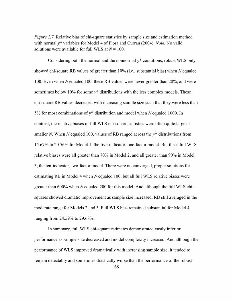
68


with normal y* variables for Model 4 of Flora and Curran (2004). Note. No valid

solutions were available for full WLS at N = 100.

Considering both the normal and the nonnormal y* conditions, robust WLS only

showed chi-square RB values of greater than 10% (i.e., substantial bias) when N equaled

100. Even when N equaled 100, these RB values were never greater than 20%, and were

sometimes below 10% for some y* distributions with the less complex models. These

chi-square RB values decreased with increasing sample size such that they were less than

5% for most combinations of y* distribution and model when N equaled 1000. In

contrast, the relative biases of full WLS chi-square statistics were often quite large at

smaller N. When N equaled 100, values of RB ranged across the y* distributions from

15.67% to 20.56% for Model 1, the five-indicator, one-factor model. But these full WLS

relative biases were all greater than 70% in Model 2, and all greater than 90% in Model

3, the ten-indicator, two-factor model. There were no converged, proper solutions for

estimating RB in Model 4 when N equaled 100, but all full WLS relative biases were

greater than 600% when N equaled 200 for this model. And although the full WLS chi-

squares showed dramatic improvement as sample size increased, RB still averaged in the

moderate range for Models 2 and 3. Full WLS bias remained substantial for Model 4,

ranging from 24.59% to 29.68%.

In summary, full WLS chi-square estimates demonstrated vastly inferior

performance as sample size decreased and model complexity increased. And although the

performance of WLS improved dramatically with increasing sample size, it tended to

remain detectably and sometimes drastically worse than the performance of the robust

69

WLS chi-square values. The complexity of the model being estimated was a major

determinant of relative bias, with the number of indicators appearing somewhat more

important than the number of factors.

Parameter estimates. Factor loadings and, when present, factor correlations

tended to be inflated in all cells of the study. As with the chi-square statistics, this bias

was generally worse for full WLS estimation, and the relative deficiency of full WLS

estimation was exacerbated as model size increased and sample size decreased. Figures

9-12 graphically depict Flora and Curran’s (2004) results for the normal y* conditions for

the RB of the factor loadings as a function of sample size. Increasing nonnormality of the

latent response variables generally resulted in increased positive bias of parameter

estimates, but these effects were relatively small in comparison to the effects of the other

independent variables. Figures 5-8 therefore convey the important aspects of the ways in

which model complexity and sample size differentially affected the performance of the

two estimation methods.

70

Figure 2.8. Relative bias of factor loadings by sample size and estimation method with

normal y* variables for Model 1 of Flora and Curran (2004).



0

2

4

6

8

10

12

100 200 500 1000

RB of Loadings

N

Model 1

full

robust

0

2

4

6

8

10

12

100 200 500 1000

RB of Loadings

N

Model 2

full

robust

71




normal y* variables for Model 4 of Flora and Curran (2004). Note. No valid solutions

were available for full WLS at N = 100.

0

2

4

6

8

10

12

100 200 500 1000

RB of Loadings

N

Model 3

full

robust

0

2

4

6

8

10

12

100 200 500 1000

RB of Loadings

N

Model 4

full

robust

72

Considering both the normal and the nonnormal y* distributions, the mean RB of

the factor loadings was in the trivial range for all cells given Model 1, although bias was

higher in general for full WLS. For Model 2, each robust WLS cell had a mean RB of

less than 3% across all sample sizes. Full WLS cells only had mean RB values in the

trivial range when N equaled 500 or 1000. When N equaled 200, all full WLS cells were

in the moderate range (6.43-8.57%) of RB for this one-factor, ten-indicator model. When

N equaled 100, all the Model 2 full WLS cells were in the substantial range of RB (10.71-

12.29%).

Given Model 3, RB of the loadings was still trivial for all robust WLS cells across

all sample sizes, in fact never rising above 3%. The average RB of the loadings was

always in the trivial range for full WLS when N equaled 500 or 1000. Full WLS cells

demonstrated trivial to moderate RB of loadings when N equaled 200, and solidly

moderate RB when N equaled 100 for this two-factor, ten-indicator model.

Robust WLS loadings still showed trivial bias across all sample sizes and y*

distributions for Model 4, the two-factor, twenty-indicator model. When N equaled 1000

for Model 4, one of the nonnormal y* distributions produced mean loadings barely into

the moderate range for full WLS, while the rest remained trivial. Full WLS biases for

loading estimates were squarely in the moderately biased range for all y* distributions

when N equaled 500. RB was substantial for the full WLS loadings of this largest model

when N equaled 200, ranging from 12.00% to 12.86%. No models had been successfully

estimated for this model with full WLS estimation when N equaled 100, and so no RB

information was available for this combination of conditions.

73

Standard errors. Flora and Curran (2004) also examined RB in the estimated

standard errors (SEs) of parameter estimates. SEs were negatively biased on average

across the entire study. As with chi-square statistics, more indicators, more factors, and

smaller sample sizes resulted in more bias. Also as with the chi-square statistics, robust

WLS showed far less bias than full WLS. Flora and Curran noted that the patterns of

independent variables that resulted in more bias of chi-square statistics were essentially

the same patterns that resulted in more bias for the SE estimates, and so they do not

present exhaustive results for this outcome. RB of the estimated standard errors for the

normal y* condition are shown in Figures 13-16. As with the chi-square statistics,

variability in y* distributions led to additional variability in bias of the SE estimates. But,

as with the chi-square statistics, there appeared to be no particular pattern to the influence

of nonnormality in y*.

Figure 2.12. Relative bias of standard errors by sample size and estimation method with


-90

-80

-70

-60

-50

-40

-30

-20

-10

0

10

100 200 500 1000

RB of SEs of Loadings

N

Model 1

full

robust

74





-90

-80

-70

-60

-50

-40

-30

-20

-10

0

10

100 200 500 1000


N

Model 2

full

robust

-90

-80

-70

-60

-50

-40

-30

-20

-10

0

10

100 200 500 1000


N

Model 3

full

robust

75


normal y* variables for Model 4 of Flora and Curran (2004). Note. No valid solutions

were available for full WLS at N = 100.

Empirical standard deviations of factor loadings. The empirical standard

deviations of parameter estimates, as opposed to their estimated standard errors or the

relative bias of these standard errors, are themselves of interest. Assuming equal bias

among competing estimators, the estimator that yields parameter estimates with the

lowest variability is preferred because it exhibits greater precision (Rigdon & Ferguson,

1991). Though not discussed by Flora and Curran (2004), figures 17-20 display the

within-cell empirical SDs of the factor loadings they obtained for the normal y*, five-

category conditions.

-90

-80

-70

-60

-50

-40

-30

-20

-10

0

10

100 200 500 1000


N

Model 4

full

robust

76

Figure 2.16. Empirical standard deviations of factor loadings by sample size and

estimation method with normal y* variables for Model 1 of Flora and Curran (2004).



0

0.02

0.04

0.06

0.08

0.1

0.12

100 200 500 1000

Empirical SD of Loadings

N

Model 1

full

robust

0

0.02

0.04

0.06

0.08

0.1

0.12

100 200 500 1000


N

Model 2

full

robust

77





Note. No valid solutions were available for full WLS at N = 100.

0

0.02

0.04

0.06

0.08

0.1

0.12

100 200 500 1000


N

Model 3

full

robust

0

0.02

0.04

0.06

0.08

0.1

0.12

100 200 500 1000


N

Model 4

full

robust

78

For Model 1, the least complex model, full WLS and robust WLS performed very

similarly. For both estimation methods, increasing sample size resulted in smaller

observed variability of the estimates of the factor loadings. Models 2 and 3 showed that

as model complexity increased, full WLS performed worse than robust WLS at the

smaller sample sizes. This difference at the smaller sample sizes was much more apparent

when Model 4, the most complex model, was estimated. When N = 500 or 1000, there

was little practical difference in the variability of the loading estimates provided by the

two methods regardless of model complexity.

Summary of Flora and Curran (2004). Flora and Curran (2004) compared the

performance of full WLS with that of robust WLS across a range of conditions of

correctly specified models. Robust WLS performed better than full WLS across all

conditions in terms of bias of chi-square statistics, bias of parameter estimates, bias of

standard errors estimates, and precision of parameter estimates. As sample size decreased

and model complexity increased, robust WLS was also much more likely to provide valid

model solutions. The superiority of the robust method was sometimes trivial with larger

sample sizes and simpler models, but was often dramatic at smaller sample sizes and with

more complex models. One limitation of Flora and Curran was that only correctly

specified models were considered. The performance of these two estimation methods

given model misspecification remains unknown.

Statement of the Problem

Ordinal data abound in applied research. Applied researchers frequently desire to

perform covariance structure analyses, including confirmatory factor analyses, using

79

these data. Robust WLS seems to have replaced full WLS as the estimation method of

choice when performing these analyses. For example, the Mplus User’s Guide

recommends the mean- and variance-adjusted robust method (known as WLSMV in

Mplus syntax) for basic applications involving categorical dependent variables other than

the testing of nested models, and the Mplus software defaults to this estimation method

for most of these analyses (Muthén & Muthén, 2005).

The performance of robust WLS has been unambiguously superior to that of full

WLS in the limited research that has been reported to date (Flora & Curran, 2004;

Muthén, du Toit, & Spisic, 1997). Robust WLS has shown significantly less inflation of

chi-square statistics, less inflation of parameter estimates, greater efficiency of parameter

estimates, and less deflation of standard error estimates. These overall performance

advantages are especially notable for smaller sample sizes and as models become more

complex.

Critically, the studies that have demonstrated the superior performance of robust

WLS have only examined correctly specified models. In fact, models might only be

perfectly specified in contrived situations such as simulation studies. As MacCallum

points out, “A critical principle in model specification and evaluation is the fact that all of

the models that we would be interested in specifying and evaluating are wrong to some

degree.” (1995, p. 17). In this context, MacCallum seems to be talking about the entire

class of threats to model validity. This includes those threats that are not necessarily

manifested by empirical failure to adequately reproduce the sample variance-covariance

matrix (e.g., wrongly specifying the direction of a causal arrow), and even those threats

80

that are not adequately addressable via any SEM technique (e.g., fundamentally nonlinear

relations among variables). But in any event, it is in many cases unlikely that a

reasonably parsimonious model specification will result in adequate reproduction of the

sample data as indexed by the chi-square statistic (e.g., Barrett, 2007; Bollen, 1989, 1993;

Kline, 1998; Mulaik, 2007). Though it is possible that a correct model may be rejected

with the chi-square statistic in applied settings due to, e.g., a type I error or a violation of

the assumptions associated with a particular estimation method, it is quite likely that in

many instances the correct model has simply not been specified.

It is therefore worthwhile to examine the performance of full WLS and robust

WLS given the specification of models that do not correspond to the population model

that yielded the sample data. This would be true even in the absence of any specific

reasons for suspecting differences in performance between these two methods in the

context of misspecification. However, there are at least two specific reasons to inquire

about the performance of these two estimation methods with misspecified models.

As previously discussed, Curran, West, and Finch (1996) examined the

performance of the S-B scaled chi-square and the ADF estimator given misspecified

models for continuous data. As nonnormality of the indicators increased, both methods

demonstrated decreasing expected values of chi-square, yet increasing levels of positive

bias. The extent to which the net effect of these dual influences resulted in increased or

decreased model rejection rates for each estimation method depended both on the

particular model estimated and on sample size.

81

As pointed out by Flora and Curran (2004), the corrections applied to the chi-

square statistics and standard error estimates in the robust WLS method are similar to the

corrections of the S-B chi-square. Similarly, it is obvious that ADF estimation is similar

to full WLS in that both methods share the burden of the large weight matrix. It is

possible then that the patterns of performance of full WLS and robust WLS estimation

will to some extent parallel the patterns exhibited by ADF and S-B scaling (respectively)

when models are misspecified. Therefore, it is desirable to elucidate the practical

consequences of nonnormality of the indicators on the power these methods have for the

rejection of misspecified models. In so doing, it is worthwhile to simultaneously consider

the tendencies of these estimators to incorrectly reject correctly specified models. Power

to reject misspecified models is only meaningful to the extent that correctly specified

models are not rejected.

A second reason to inquire about the possibility of a change in the relative

performance of these two estimation methods when models are misspecified is related to

the robust WLS innovation of using the diagonal weight matrix Wdiag in place of the full

weight matrix during parameter estimation. In the iterative process of attempting to

minimize the discrepancies between the sample polychoric correlations and their model-

implied counterparts, either estimation method is expected to encounter more difficulty in

converging on parameter estimates when a model is misspecified. The off-diagonal

elements of the full WLS asymptotic covariance matrix, Wfull, are generally unstable

regardless of model specification, and this has been shown to be a hindrance to accuracy

of parameter estimates when models are correctly specified. Nevertheless, the robust

82

WLS method of simply replacing these off-diagonal elements with zeros does discard

information. It is possible that these off-diagonal become either more harmful or more

useful when incorrect models are specified.

Purpose of the Study

This simulation study examined the extent to which the superior performance of

robust WLS over full WLS extended to situations in which models are misspecified. The

inclusion of misspecified models was an important, novel addition to previous research

on these estimation methods. Design factors with levels representing different sample

sizes and various relevant distributional characteristics of observed ordinal variables were

included in order to begin to qualify any observed differences in the performance of these

two methods. Bias in chi-square estimates, parameter estimates, and estimated standard

errors were outcomes of interest, as was the relative precision of the parameter estimates.

83

Chapter III: Method

A simulation study was performed in order to examine the extent to which the

superior performance of robust WLS over full WLS extended to situations in which a

model is misspecified. Distributional shape of scores on the ordinal indicator variables,

sample size, and model specification are the design factors that were manipulated in

addition to estimation method. The two estimation methods were compared in terms of

the bias of their chi-square values, their model rejection percentage, the bias of their

parameter estimates, the precision of their parameter estimates, and the bias of their

parameter estimates’ standard error estimates.

Population Model

The population model had two correlated factors and eight total indicators (Figure

3.1). This model was similar to the population model used by Curran, West, and Finch

(1996), except that there were two factors instead of three, and four indicators per factor

instead of three. The population variance of each factor was 1.0. Therefore the covariance

between the factors was the same as the correlation, which was .30. Each factor had three

latent, continuous y* indicators that loaded exclusively on that factor with a value of .70.

Two more latent, continuous y* indicators loaded .70 on one factor and cross loaded .35

on the other. These loadings and cross loadings were of the same size as those of Curran

et al. Loadings of .70 are moderate in size and frequently appear in other CFA simulation

studies (e.g., Flora & Curran, 2004; Potthast, 1993; Rigdon & Ferguson, 1991). Because

the population variance of each latent, continuous y* indicator set at 1.0 and the

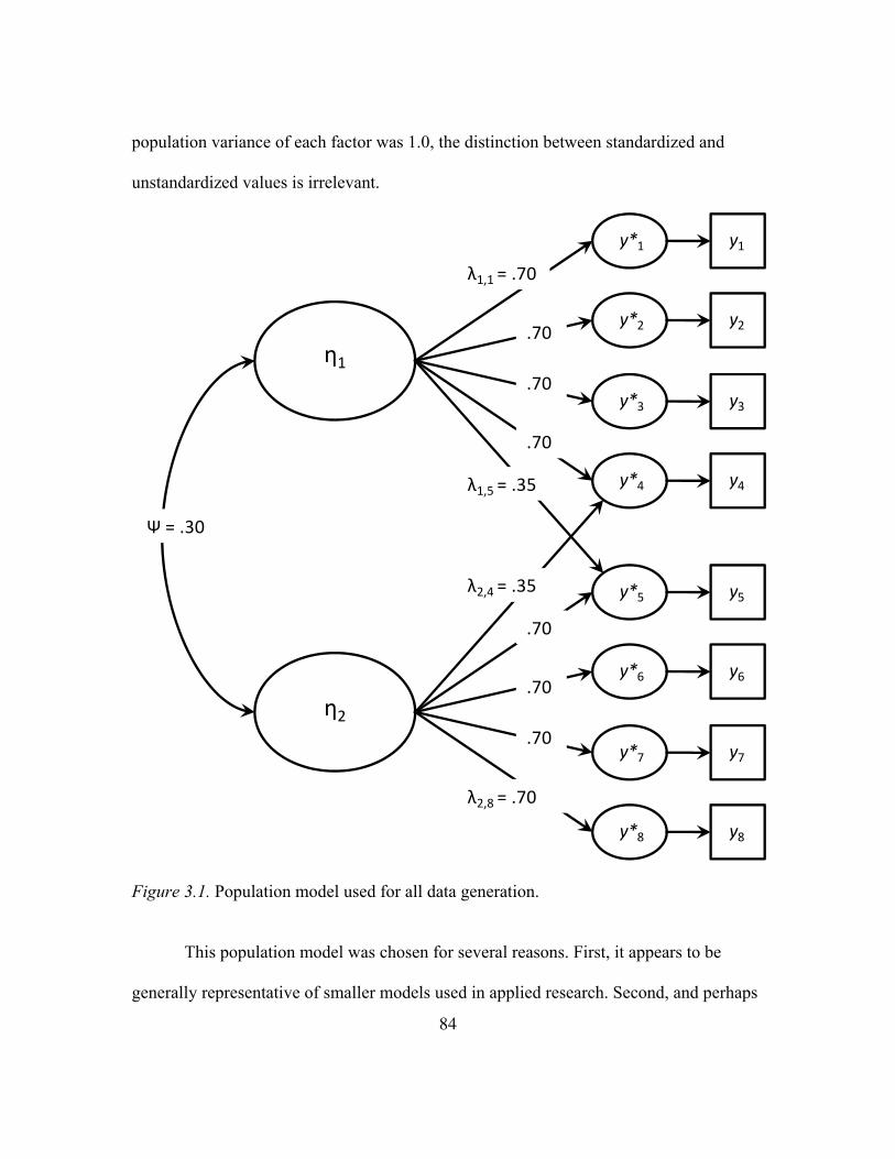
84

population variance of each factor was 1.0, the distinction between standardized and

unstandardized values is irrelevant.

Figure 3.1. Population model used for all data generation.

This population model was chosen for several reasons. First, it appears to be

generally representative of smaller models used in applied research. Second, and perhaps

y7y*7

y8y*8

y5y*5

y6y*6

y3y*3

y4y*4

y1y*1

y2y*2

η1

η2

Ψ = .30

λ2,8 = .70

λ1,1 = .70

λ1,5 = .35

λ2,4 = .35

.70

.70

.70

.70

.70

.70

85

due to the previous reason, this model shares features with many models in the existing

CFA simulation literature. Besides its aforementioned similarity to Curran, West, and

Finch (1996), its two-factor, eight-indicator form partially or completely overlaps with

models appearing in many notable CFA simulation studies (e.g., Babakus, Ferguson, &

Jöreskog, 1987; Chou, Bentler, & Satorra, 1991; Flora & Curran, 2004; Muthén &

Kaplan, 1985; Muthén & Kaplan, 1992; Potthast, 1993; and Rigdon & Ferguson, 1991).

A final reason for the selection of this model was that it provided opportunities for

realistic misspecification (i.e., the omission of true cross loadings and the inclusion of

false cross loadings) with minimal complication.

Design Factors

In addition to estimation method, for which the two levels were full WLS and

robust WLS, design factors of sample size, indicator distribution, and model specification

were also included.

Sample Sizes

Sample sizes should be selected not only so that results are useful to applied

researchers, but also so that results are comparable with prior research. Sample sizes of

100, 200, 500, and 1000 frequently appeared in simulation studies of CFA (e.g., Babakus,

Ferguson, & Jöreskog, 1987; Chou, Bentler, & Satorra, 1991; Curran, West, & Finch;

Flora & Curran, 2004; Hu, Bentler, & Kano, 1992; Muthén & Kaplan, 1985; Muthén &

Kaplan, 1992; Potthast, 1993; Rigdon & Ferguson, 1991) and also covered much of the

range of sample sizes likely to be found in applied work (e.g., Breckler, 1990). Though N

86

= 100 is likely to be inappropriately small in many applied contexts, especially if full

WLS is used, it met the two previous criteria and was therefore included.

Distributions of Observed Variables

Although ordered categorical variables are fundamentally nonnormal by virtue of

their discrete nature (Bollen, 1989; Muthén, 1984), these variables are also likely to be

nonnormal as measured by skewness and kurtosis (Kaplan, 2000; Muthén & Kaplan,

1985). Departures from the basic bell-curve shape of normality, particularly kurtosis,

accounted for much of the poor performance exhibited by estimators when categorical

observed variables were present (DiStefano, 2002; Finney & DiStefano, 2006; Muthén &

Kaplan, 1992; Potthast, 1993; see chapter II). For this reason it was important to include

conditions representing various levels of skewness and kurtosis of the ordered categorical

indicators. Note that skewness and kurtosis are to some extent dependent, and thus could

not be treated as two separate factors and then crossed with each other.

Conditions representing seven separate observed variable distributions were

included. All distributions had five categories. Both to retain comparability with previous

studies and because previous studies seemed to cover the spectrum of ordered categorical

variable distributions that are likely to be observed by applied researchers, six of these

seven distributions were drawn from prior research (Muthén & Kaplan, 1985; Muthén &

Kaplan, 1992; Potthast, 1993). The seventh distribution was of mixed skew. Two

indicators of each factor were shaped exactly like the moderate ceiling distribution. The

other two were the mirror image of this, i.e. shaped to have a moderate floor effect. For

each distribution, Table 3.1 displays the skew, kurtosis, and the four thresholds (t1 – t4)

87

that yield this distribution when these thresholds are used to segment the standard normal

distribution. Figure 3.2 displays the shape of each of the distributions as a histogram.

Table 3.1

Skew, Kurtosis, and Standard Normal Distribution Threshold Sets for Indicator

Distributions

Distribution Skew Kurtosis t1 t2 t3 t4

Normal 0.00 0.00 -1.645 -0.643 0.643 1.645

Rectangular 0.00 -1.30 -0.842 -0.253 0.253 0.842

Mild ceiling 0.74 -0.33 -1.645 -1.036 -0.385 0.385

Moderate ceiling 1.22 0.85 -1.881 -1.341 -0.772 0.050

Severe ceiling 2.03 2.90 -1.645 -1.282 -1.036 -0.674

Symmetric,

leptokurtic 0.00 2.70 -1.645 -1.150 1.150 1.645

Mixed skew ±1.22 0.85 ±1.881 ±1.341 ±0.772 ±0.050

88

Figure 3.2. Histograms of the six indicator distributions. Note. The mixed skew condition

utilizes the moderate ceiling distribution and its mirror image.

Model Specifications

Though a single population model was used to generate data, four different

models were estimated. Although the population model in this study differed somewhat

from that of Curran, West, and Finch (1996), these four specifications essentially

corresponded to the four model specifications chosen by Curran et al. For all estimations,

each factor was identified by fixing its variance to 1.0 instead of fixing a loading.

In the first condition, the population model was correctly specified. This

essentially allowed for an attempted replication of the findings for the normal y*

89

conditions of Flora and Curran (2004), but with a different population model. Including

this condition also allowed the establishment of “baseline” performance so that changes

in performance given misspecification could be observed.

The second model specification had the correct model nested within it, but

included two superfluous cross loadings. These cross loadings had a value of zero in the

population, and one such loading was estimated for each of the two factors. Curran et al.

(1996) noted that a misspecification involving this kind of inclusion should not bias

parameter estimates, and could therefore be considered to be technically correctly

specified. It is also possible to regard this model as incorrectly specified in that it is

overparameterized. In either case, parameters that are zero in the population should be

estimated as zero, and expected values of estimates of nonzero parameters should equal

the population values. The expected value of chi-square for this model is equal to its

degrees of freedom, 15.

The third and fourth specifications represented unambiguously misspecified

models. The third model specification differed from the correctly specified model in that

the two cross loadings were omitted. This condition simulated a situation in which a

researcher optimistically models each observed variable as an indicator of only one

factor, when in fact two of the indicators also measured the other factor to some extent.

The fourth specification also omitted these cross loadings, but included the two

superfluous cross loadings of the second model. This represented a situation in which a

researcher misjudged which two indicators cross load.

90

Design Summary

Conditions representing two estimators, four model specifications, four sample

sizes, and seven distributions of observed indicator variables were completely crossed.

Thus there were 2 × 4 × 4 × 7 = 224 individual combinations of conditions. From the

perspective of experimental design, each unique combination of conditions can be called

a cell, and each individual incidence of model estimation on simulated data is an

observation. The same simulated data were used for both full and robust WLS estimation.

Data Generation

The Mplus software package (Muthén & Muthén, 2005) was used to generate

observations from the overall population model for each replication of the study,

according to the specific distribution of observed variables and the specific sample size

required. Because the same population model was used across the entire design, the only

aspects of the data that changed across conditions were the indicator variable shape and

the sample size.

It is important to remember that population models for ordered categorical data

pertain to the y* variables, and not the observed ordered categorical variables (i.e., to ∑*

and not ∑; Bollen, 1989, Muthén, 1984; Muthén & Kaplan, 1985; Muthén & Muthén,

2005). As such, each simulated observation generated by the Mplus package first existed

in the form of values on each of the eight continuous y* variables. It is the population

covariance pattern of these eight y* variables that corresponded to the population CFA

model. Each of the latent y* variables in this study was generated from a population

91

where the variance of each y* is 1.0. This is consistent with the situation in which an

applied researcher is using full or robust WLS with ordered categorical data and is

expecting that a polychoric correlation matrix will be estimated from these data for

analysis. The simulated observed ordered categorical data values themselves were

determined at the last step of data generation by applying the appropriate set of thresholds

to the generated y* values.

As an example, consider any of the 32 design cells in which the ordinal y

indicator variables were approximately normally distributed. A single simulated sample

of data to which a model was fit first took the form of N z-like values for the eight y*

variables, where N was a level of the sample size factor; 100, 200, 500, or 1000. The four

thresholds for the rectangular condition were -0.842, -0.253, 0.253, and 0.842. The

corresponding eight y integer values could have ranged from 0 to 4, and were determined

by where y* fell in relation to the thresholds. For example, if y* happened to fall below

-0.842, then y would have been 0. If y* was above -0.842 but beneath -0.253, y would

have been 1, etc. In this way, the N groups of eight y* values were converted to N groups

of eight y values ranging from 0-4. This approach to data generation is consistent with

prior research involving SEM with ordered categorical data, and also with the concept of

the latent variable formulation (Muthén & Kaplan, 1985; Muthén & Muthén, 2005).

Within any particular combination of indicator distribution, sample size, and model

specified, the same random seed was used to generate data. This ensured that direct

comparisons of full WLS and robust WLS were always based on the same sample data.

92

The internal Monte Carlo analysis feature of Mplus (Muthén & Muthén, 2005)

allowed data to be generated according to the population model, ordinalized according to

the specific indicator distribution desired, and analyzed with the estimation method and

model specification appropriate to that cell of the design. Chi-square statistics, parameter

estimates, and estimated SEs were then automatically written to a text file. Though this

feature of Mplus greatly assisted in conducting this simulation study, it was still

necessary to produce the appropriate input document for each of the 224 cells of the

design. In order to accomplish this, the R programming environment (R Foundation for

Statistical Computing, 2007) was used to automatically write a separate Mplus input

document for each of the 224 conditions, as well as a DOS batch file that automatically

ran each of the files. The R environment was again used to aggregate the 224 separate

output files of chi-square estimates and sample statistics for analysis in Excel and SPSS.

Outcomes of Interest

Relative bias (RB; Hoogland & Boomsma, 1998) served as the dependent

measure for many outcomes of interest in this study:

RB =ˆ θ − θ

θ

∗100 , (3.1)

where θ is the expected value of an outcome. RB is generally interpreted to be trivial in

magnitude when less than 5%, moderate when ranging from 5 – 10%, and substantial

when greater than 10% (Bandalos, 2006; Curran, West, & Finch, 1996; Flora & Curran,

2004; Kaplan, 1989).

93

Chi-Square Statistics

For the conditions in which the model was correctly specified, θ in Equation 3.1

for chi-square was equal to the degrees of freedom for the chi-square statistic. Difficulties

arose, however, when a model was misspecified. In order to produce expected values for

full WLS chi-squares given model misspecification, it was necessary to adapt the

technique of Curran, West, and Finch (1996, Appendix) to this situation. It was necessary

to apply this technique 56 times; once for each combination of indicator thresholds,

sample size, and model misspecification. This technique, as adapted slightly for use with

ordinal variables, was as follows:

1) A very large (100,000 cases) sample of simulated, continuous data was

generated according to the population model for the latent y* variables. This same data

set was used for each of the 14 occasions where a model misspecification was applied

with a particular threshold set.

2) The thresholds of interest were applied in order to segment the continuous y*

variables into ordered categorical factor indicators.

3) Both of the incorrectly specified models were estimated with this sample of

simulated ordered categorical data using the full WLS estimator.

4) The minimum of the fit function (Equation 2.16) was extracted from the chi-

square value resulting from each of these model estimations (Equation 2.17). Because the

full WLS chi-square value equals 2NFWLS, the minimum of the fit function is therefore χ2

/2N. Because N = 100,000, the minimum of the fit function was thus χ2 /200,000.

94

Because there were two misspecifications of interest and seven indicator shapes of

interest, a total of 14 models were estimated and thus 14 minima were extracted.

5) For each of the four sample sizes of interest (100, 200, 500, and 1000), each fit

function minimum was re-scaled according to the sample size minus 1. For example,

when the expected value of chi-square was desired for an instance where N would equal

500, then the re-scaled value was 2 × 499 × FWLS (see Equation 2.17). This step was

performed 56 times; once for each combination of sample size, indicator shape, and

model misspecification.

6) These values were then added to the degrees of freedom for the appropriate

misspecified model. The resulting value was a large sample empirical estimate of the

expected value of chi-square given a particular model misspecification, estimation

method, and distributional shape of the observed variables.

It was of course desirable to compare full WLS directly with robust WLS in order

to evaluate the relative quality of their performances. Therefore, computing expected

values of chi-square separately for the two methods did not make sense. Because of the

theoretical soundness of full WLS with large samples, and because full WLS does in fact

begin to perform acceptably under many circumstances when N = 1000 (see chapter II),

the full WLS values resulting from the method described above were used as expected

values of chi-square. As discussed above, the large sample size of 100,000 was used to

generate expected values.

An additional, substantial difficulty in evaluating bias in chi-square statistics

arose because the degrees of freedom for robust WLS do not usually equal the

95

conventional model degrees of freedom, but instead are determined empirically from the

data (Muthén, du Toit, & Spisic, 1997). For this reason, degrees of freedom may vary

across estimations of the same model using robust WLS. The p-values and not the chi-

square values themselves are what are intended for interpretation by the applied

researcher, and chi-square difference testing of nested models is not possible with robust

WLS (Muthén & Muthén, 2005).

Direct comparison of the p-values from each method rather than the chi-square

statistics was an impractical alternative. Because p-values are nonlinearly related to chi-

square values, interpretable differences in chi-square often equate to p-values that differ

by many orders of magnitude. One alternative was to use the robust WLS p-values in

conjunction with the conventional model degrees of freedom, i.e. the same model degrees

of freedom that applied to full WLS estimations, in order to triangulate comparable chi-

square-scale values for robust WLS by using an inverse chi-square distribution function.

Unfortunately, the extremely low p-values that sometimes manifested at the larger sample

sizes could not always be represented in applications such as Excel and SPSS and/or

processed by the inverse chi-square distribution functions of these programs.

Instead, an imperfect method that made use of the mean and variance of the null

hypothesis chi-square distribution was used to rescale the robust values to the full WLS

scale. Ordinary chi-square distributions have a mean equal to their degrees of freedom

and a variance that is 2df. In general, when a model is estimated it is the relative rarity or

commonness of the particular chi-square value relative to the model degrees of freedom

that determines the plausibility of the model specification. While the p-value is

96

commonly used to index the commonness or rarity of this chi-square value, one could

also index the chi-square value according to the mean and variance of its ostensible

distribution given the null hypothesis of correct model specification. Robust WLS chi-

square values were thus transformed to apply to the conventional model degrees of

freedom by using a simple z-score procedure. For example, if a robust estimation

repetition provided a chi-square of 19 with 12 degrees of freedom, the value of 19 is at z

= 2.02 according to the mean and variance of the ostensible chi-square distribution given

the null hypothesis of model fit. If the ordinary degrees of freedom for the estimated

model equaled 17, then the value of 25.36 would served as the equivalent full WLS scale

value of chi-square.

This method is imperfect because chi-square distributions are asymmetrical, and

the degree of asymmetry depends on the degrees of freedom. For this reason, the p-value

for a chi-square of 19 with 12 degrees of freedom does not exactly equal the p-value of a

chi-square of 25.36 with 17 degrees of freedom. However, careful examination of the

performance of this procedure on data generated for this purpose suggested that only

minimal bias was introduced. It was also possible to use the previously mentioned inverse

chi-square function imputation technique to equate full and robust WLS chi-squares

based on p-values at the smaller sample sizes for most indicator distributions. When RB

values of chi-square were calculated for each method and viewed in the graphical formats

used in chapter IV, values appeared to be essentially the same. Additionally, results

regarding the proportion of significant chi-squares at p < .01 (presented in chapter IV)

were consistent with findings from the z-score procedure. Robust WLS chi-square values

97

were therefore transformed to the full WLS scale using this method. These transformed

values were used for the calculation of RB of chi-square statistics for the robust method.

Full WLS chi-squares required no transformation.

The more conventional approach of examining percentages of model rejections

was also utilized. The criterion of α = .01 was used instead of .05 because the chi-square

test is popularly regarded as a stringent criterion for model evaluation. Thus, a particular

repetition counted as a rejection if the associated p-value was less than .01. The

proportion of rejected models for each cell of the study is reported in chapter IV.

Parameter Estimates

Factor loadings and factor correlations were examined using RB. RB for factor

correlations and factor loadings are presented separately, and further distinctions are

made among factor loadings. One representative loading from each class of loadings is

examined. For example, when the model is correctly specified λ1,1 is indistinguishable in

terms of both expected value and function within the model from λ1,2, λ1,3, λ2,6, λ2,7, and

λ2,8 (see figure 3.1) but not λ1,4 and λ2,5. These two loadings share with the previous

loadings the expected value of .70, but the two indicator variables to which these loadings

apply are qualitatively different in that they measure both factors. Therefore, λ1,4 and λ2,5

are members of a different class. Similarly, the cross loadings λ1,5 and λ2,4 are members of

yet another class. Findings for one loading from each separate class are presented. Values

of θ used in Equation 3.1 for any particular parameter estimate were drawn directly from

the population model. Observed RB across conditions of the study for each of these types

of parameters is presented graphically and discussed in chapter IV.

98

Estimated Standard Errors

For any particular estimated parameter, the empirical standard deviation of the

parameter estimates was calculated within each cell. For each parameter estimate, this

value then served as the expected value for the calculation of RB of the estimated

standard errors (SEs). The mean of the standard errors provided by the estimation method

for that particular parameter for that particular cell then served as ˆ θ for use in Equation

3.1. As with the analyses of the parameter estimates themselves, RB of the SEs for each

type of parameter are considered separately in chapter IV.

Empirical Standard Errors

The values used as θ for evaluation of the estimated SEs are interesting in their

own right. In general, estimates with less variability are more desirable than estimates

with more variability, because the former are more precise. For this reason, these

empirical standard deviations are also graphed and discussed.

99

Chapter IV: Results

This chapter presents the results of the simulation study. Rates of nonconvergence

and improper solutions are first addressed. The expected values of chi-square resulting

from the large sample approximation method described in the previous chapter are then

presented for the two misspecified models. Next, the relative biases of chi-square values

for the two estimation methods across conditions of the study are presented for each

estimation method, followed by the corresponding proportions of model rejections at α =

.01. Relative biases of parameter estimates across conditions are then presented, followed

by the precision of these parameter estimates as indicated by their empirical standard

deviations. Finally, relative biases of estimated standard errors are given. The empirical

standard deviations within each cell served as the standards (i.e., as the values of θ in

Equation 3.1) by which RB of these estimated standard errors were evaluated.

Nonconvergent and Inadmissible Solutions

There were very few convergence failures across conditions of the study. The

highest rate of 3.48% occurred for the N = 100, severe ceiling cell where full WLS was

used to estimate the df = 17 misspecified model. The second highest rate of 1.21%

occurred for the N = 100, leptokurtic cell where full WLS was used to estimate the df =

17 misspecified model. Across conditions, rates of nonconvergence were usually zero at

N = 200, and always zero at N = 500 and N = 1000. In general, nonconvergence was more

likely with full WLS estimation, more kurtotic indicators, and either the df = 17

misspecified model or the overspecified model.

100

For most basic SEM applications involving categorical dependent variables and

full WLS or robust WLS estimation, including the single-group CFA models simulated in

this study, Mplus defaults to what the software authors refer to as the delta

parameterization (L. K. Muthén & B. O. Muthén, 2005). When models like those in the

present study are estimated with this parameterization, variances of the latent response

variables (y*s) are set to 1.0 (B. O. Muthén, 1998-2004; L. K. Muthén, personal

communication, August 8th

, 2009). Additionally, models in the present study were

identified for estimation by fixing each factor variance at 1.0 rather than fixing a factor

loading. Converged but inadmissible solutions were therefore recognized as those where

the factor correlation was greater than 1.0, an uncomplicated loading was greater than

1.0, or where values of a loading, cross loading, and the factor correlation together

suggested a negative error variance for a latent response variable. For each cell of the

study, Table 4.1 presents the percentage of solutions that not only converged, but were

also admissible.

101

Tab

le 4

.1

Per

centa

ges

of

Adm

issi

ble

Solu

tions

Acr

oss

Stu

dy

Condit

ions

Model

N

= 1

00

N

= 2

00

N

= 5

00

N

= 1

000

Full

WL

S

Robust

WL

S

Full

WL

S

Robust

WL

S

Full

WL

S

Robust

WL

S

Full

WL

S

Robust

WL

S

Corr

ect

N

orm

al

96.7

1

99.1

2

99.9

0

100

100

100

100

100

R

ecta

ngula

r 97.8

0

99.8

0

100

100

100

100

100

100

M

ild C

eili

ng

97.3

8

99.5

8

100

100

100

100

100

100

M

oder

ate

Cei

ling

94.4

3

98.2

9

100

100

100

100

100

100

S

ever

e C

eili

ng

70.0

3

88.7

3

96.8

9

98.9

0

100

100

100

100

L

epto

kurt

ic

74.4

2

90.1

9

98.3

0

99.8

0

100

100

100

100

M

ixed

Skew

91.3

7

96.7

1

99.2

9

99.7

0

100

100

100

100

Over

spec

ifie

d

N

orm

al

93.3

0

98.4

6

99.8

0

100

100

100

100

100

R

ecta

ngula

r 94.3

0

98.3

0

100.0

0

100

100

100

100

100

M

ild C

eili

ng

93.3

1

98.2

2

99.9

0

100

100

100

100

100

M

oder

ate

Cei

ling

89.8

6

96.0

0

99.2

9

99.8

0

100

100

100

100

S

ever

e C

eili

ng

58.4

2

81.3

0

91.9

8

97.3

9

99.9

0

100

100

100

L

epto

kurt

ic

66.3

7

82.8

0

96.0

0

98.6

0

100

100

100

100

M

ixed

Skew

86.3

0

93.2

9

98.9

9

99.6

0

100

100

100

100

102

Tab

le 4

.1 (

Conti

nued

)

Model

N

= 1

00

N

= 2

00

N

= 5

00

N

= 1

000

Full

WL

S

Robust

WL

S

Full

WL

S

Robust

WL

S

Full

WL

S

Robust

WL

S

Full

WL

S

Robust

WL

S

df

= 1

9

Mis

- N

orm

al

57.6

3

43.2

5

82.6

8

51.5

5

98.5

0

61.6

0

100

77.4

0

spec

ifie

d

Rec

tangula

r 65.5

0

48.5

0

89.5

0

52.3

0

99.4

0

65.9

0

100

78.9

0

M

ild C

eili

ng

61.7

2

46.4

4

85.2

9

52.1

5

99.4

0

63.7

0

100

78.3

0

M

oder

ate

Cei

ling

52.4

3

43.2

9

81.1

0

50.3

0

98.0

0

60.2

0

100

72.7

0

S

ever

e C

eili

ng

39.6

1

41.9

3

59.9

2

44.9

9

87.7

0

51.4

0

98.5

0

65.2

0

L

epto

kurt

ic

38.9

2

36.6

0

55.3

6

40.0

4

82.5

0

46.8

0

96.7

0

59.9

0

M

ixed

Skew

45.6

2

38.7

7

69.7

3

45.0

1

94.2

0

57.2

0

99.4

0

69.1

0

df

= 1

7

Mis

- N

orm

al

38.3

1

48.9

6

69.8

7

67.7

7

96.0

0

94.6

0

99.8

0

99.3

0

spec

ifie

d

Rec

tangula

r 41.2

0

52.2

0

75.1

0

73.3

0

96.2

0

96.0

0

99.8

0

100

M

ild C

eili

ng

38.9

1

50.0

0

71.5

7

71.7

7

95.4

0

94.2

0

99.6

0

99.7

0

M

oder

ate

Cei

ling

33.4

3

44.8

6

66.7

7

67.2

8

93.0

0

92.3

0

99.4

0

99.3

0

S

ever

e C

eili

ng

19.0

5

31.1

3

38.6

8

45.4

9

79.5

0

75.4

0

95.2

0

92.4

0

L

epto

kurt

ic

24.4

8

28.6

7

44.5

4

46.4

5

83.3

0

75.5

0

97.9

0

93.1

0

M

ixed

Skew

31.6

4

40.6

8

62.6

6

60.0

4

91.7

0

86.3

0

99.5

0

98.3

0

103

In general, larger sample sizes and indicators with less kurtosis and skew were

associated with higher rates of valid solutions. Rates of valid solutions were also clearly

higher when the model was correctly specified or overspecified. When differences

emerged between the two estimation methods given these two model specifications, it

was almost always robust WLS that yielded larger percentages of valid solutions at any

particular combination of sample size and indicator shape. Interestingly, robust WLS

tended to show lower convergence rates than full WLS for the df = 19 misspecification,

but often higher rates given the df = 17 misspecification.

Expected Values of Chi-Square for Misspecified Models

The expected values of the full WLS chi-square that were calculated according to

the adapted method of Curran, West, and Finch (1996; see Appendix) with a simulated

sample size of 100,000 are presented in figures 4.1 and 4.2 for the df = 19 and df = 17

misspecified models, respectively. In order to verify the performance of this method,

similar expected values were also calculated for the correctly specified model and the

overspecified model. Across all conditions of sample size and indicator distribution, these

calculated expected values were only trivially larger than the model degrees of freedom,

never by more than .18. The degree of this trivial overestimation was positively

associated with sample size, because N is directly involved in the computation of these

expected values (see Equation 2.17). For the same reason, the differences in expected

values across indicator distributions became more pronounced with increasing N while

their rank order within any particular N remained constant.

Figure 4.

WLS

misspecified model.

Figure 4.1. Expected values across sample sizes and indicator distributions of the full

WLS χ2 calculated using the large sample fit function extraction technique for the

misspecified model.

Expected values across sample sizes and indicator distributions of the full

calculated using the large sample fit function extraction technique for the

misspecified model.



104








calculated using the large sample fit function extraction technique for the df = 19

= 19

Figure 4.

WLS

misspecified model.

varian

of freedom equal to the model degrees of freedom to which these values apply might

allow a coarse frame of reference. Whereas the mean of a chi

to its degrees of freedom, the variance is 2

degrees of freedom therefore have standard deviations of 6.16 and 5.83, respectively. At

an alpha level of .05, critical values of the chi

17 are 30.14 and 27.59, respectively. If the full WLS chi

relative to these expected values, there would apparently be little power to consistently

reject these misspecified models when

Figure 4.2. Expected value

WLS χ2 calculated using the large sample fit function extraction technique for the

misspecified model.

These expected values are point estimates. Information about their expected

variance is not available. However, the variance of chi











misspecified model.


ce is not available. However, the variance of chi









s across sample sizes and indicator distributions of the full











reject these misspecified models when N

105







to its degrees of freedom, the variance is 2df. Chi-square distributions with 19 and 17


an alpha level of .05, critical values of the chi-square distribution when



N = 100. When




ce is not available. However, the variance of chi-square distributions with degrees


allow a coarse frame of reference. Whereas the mean of a chi-square distribution is equal

square distributions with 19 and 17


square distribution when

17 are 30.14 and 27.59, respectively. If the full WLS chi-square performed without bias


= 100. When N = 200, dif




square distributions with degrees


square distribution is equal



square distribution when df = 19 and

square performed without bias


= 200, differences among the


calculated using the large sample fit function extraction technique for the df = 17







= 19 and df =

square performed without bias


ferences among the

= 17




106

observed variable distributions become more relevant. Power to reject these models with

the leptokurtic indicators or the indicators with the severe ceiling effect appears suspect.

If the full WLS chi-square values were without bias, power to reject these models at N =

500 would likely be adequate even for these troublesome distributions.

Model Chi-Square Values

Relative Bias of Chi-square Values

For the correctly specified model and the overspecified model, the conventional

model degrees of freedom served as expected values for the calculation of RB of chi-

square values. For the two misspecified models, the large sample estimates of full WLS

expected chi-squares served as the expected values. As discussed in chapter III, degrees

of freedom supplied by the robust WLS model estimations were used to rescale the robust

chi-squares to the ordinary model degrees of freedom. This procedure produced chi-

square estimates on the scale of full WLS for each replication where robust WLS was the

estimator. These approximations then served as �� in equation 3.1 for the estimation of

chi-square bias for each robust replication. For robust WLS chi-square values, bias is a

term of convenience when used in regards to these misspecified models. The calculated

RB for robust WLS chi-square values is an indicator of performance relative to the full

WLS theoretical standard rather than bias in the strict sense of the word.

Figures 4.3, 4.4, 4.5, and 4.6 display mean RB of full WLS chi-square statistics

and the calculated RB of the rescaled robust chi-square values for the correctly specified

model, the overspecified model, the misspecified model with 19 degrees of freedom, and

the misspecified model with 17 degrees of freedom, respectively.

107

Fig

ure

4.3

. M

ean r

elat

ive

bia

s of

chi-

squar

e st

atis

tics

for

the

corr

ectl

y s

pec

ifie

d m

od

el.

-505

10

15

20

25

30

35

40

45

50

55

60

Fu

llR

ob

ust

Fu

llR

ob

ust

Fu

llR

ob

ust

Fu

llR

ob

ust

N =

10

0N

= 2

00

N =

50

0N

= 1

00

0

% Relative Bias

Sa

mp

le S

ize

by

Est

ima

tio

n M

eth

od

No

rma

lR

ect

an

gu

lar

Mil

d C

eil

ing

Mo

de

rate

Ce

ilin

gS

eve

re C

eil

ing

Lep

toku

rtic

Mix

ed

Ske

w

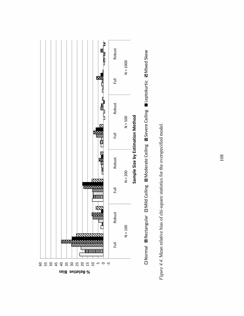
108

Fig

ure

4.4

. M

ean r

elat

ive

bia

s of

chi-

squar

e st

atis

tics

for

the

over

spec

ifie

d m

odel

.

-505

10

15

20

25

30

35

40

45

50

55

60

Fu

llR

ob

ust

Fu

llR

ob

ust

Fu

llR

ob

ust

Fu

llR

ob

ust

N =

10

0N

= 2

00

N =

50

0N

= 1

00

0

% Relative Bias

Sa

mp

le S

ize

by

Est

ima

tio

n M

eth

od

No

rma

lR

ect

an

gu

lar

Mil

d C

eil

ing

Mo

de

rate

Ce

ilin

gS

eve

re C

eil

ing

Lep

toku

rtic

Mix

ed

Ske

w

109

Fig

ure

4.5

. M

ean r

elat

ive

bia

s of

chi-

squar

e st

atis

tics

for

the

mis

spec

ifie

d m

odel

wit

h d

f =

19.

0

10

20

30

40

50

60

70

80

90

10

0

11

0

Fu

llR

ob

ust

Fu

llR

ob

ust

Fu

llR

ob

ust

Fu

llR

ob

ust

N =

10

0N

= 2

00

N =

50

0N

= 1

00

0

% Relative Bias

Sa

mp

le S

ize

by

Est

ima

tio

n M

eth

od

No

rma

lR

ect

an

gu

lar

Mil

d C

eil

ing

Mo

de

rate

Ce

ilin

gS

eve

re C

eil

ing

Lep

toku

rtic

Mix

ed

Ske

w

110

Fig

ure

4.6

. M

ean r

elat

ive

bia

s of

chi-

squar

e st

atis

tics

for

the

mis

spec

ifie

d m

odel

wit

h d

f =

17.

0

10

20

30

40

50

60

70

80

90

10

0

11

0

Fu

llR

ob

ust

Fu

llR

ob

ust

Fu

llR

ob

ust

Fu

llR

ob

ust

N =

10

0N

= 2

00

N =

50

0N

= 1

00

0

% Relative Bias

Sa

mp

le S

ize

by

Est

ima

tio

n M

eth

od

No

rma

lR

ect

an

gu

lar

Mil

d C

eil

ing

Mo

de

rate

Ce

ilin

gS

eve

re C

eil

ing

Lep

toku

rtic

Mix

ed

Ske

w

111

Given the correct or overspecified model, the performance difference between

these two estimation methods is clear. Patterns of bias are very similar for these two

model specifications, with less overall bias at smaller sample sizes for the overspecified

model. For both of these models at N = 200 and above, robust WLS chi-square values

showed inflation in the trivial range, except for the severe ceiling condition given the

correctly specified model at N = 200. Full WLS chi-square values were always

substantially inflated for these two models when N equaled 100 or 200. Across sample

sizes, peakedness of the indicator distributions was especially detrimental to the

performance of full WLS. The worst performances usually occurred with the severe

ceiling and leptokurtic distributions. Even when N equaled 1000, full WLS chi-squares

for both of these models were inflated above the trivial threshold given the severe ceiling

distributions. In contrast, asymmetry rather than peakedness caused the most problems

for robust WLS, although these problems were minor compared to those of full WLS.

The two misspecified models highlighted a very interesting performance

difference between these two estimation methods. With increasing sample size, positive

chi-square bias decreased for full WLS. This mirrored the pattern observed for the correct

and overspecified models. For robust WLS however, increasing N caused increasing bias

of chi-square values relative to the large sample full WLS standards for bias. It is again

worth noting that this is not actually bias in the literal sense. It is instead an index of the

power of robust WLS to reject misspecified models relative to the theoretically unbiased

approximated full WLS standard. This demonstrated that robust WLS chi-squares have

much greater specificity to the validity of the model. Robust WLS gave less inflation of

112

chi-square statistics when the model was correctly specified, yet more power to reject a

misspecified model. At N = 100, full WLS showed greater power to reject the

misspecified models for some indicator distributions. However, this seemingly desirable

property appeared to be the result of full WLS indiscriminately inflating chi-square at

smaller N, irrespective of the correctness of model specification. Relatedly, the power of

robust WLS was lowest across sample sizes for the two least normal distributions, severe

ceiling and leptokurtic. Full WLS had its highest power for these distributions, though

this must again be understood in light of the full WLS inflation of chi-square for these

distributions given the correctly specified and overspecified models.

Proportions of Statistically Significant Chi-Square Values

Figures 4.7, 4.8, 4.9, and 4.10 display the proportions of statistically significant

chi-squares for each of the four models across conditions. If the chi-square statistics were

performing as desired, the proportion of statistically significant results would be nearly

equal to .01 across conditions for both the correctly specified and the overspecified

models. The chi-square inflation demonstrated by full WLS for these two models at N =

100 and N = 200 corresponded to substantially greater numbers of model rejections, with

the severe ceiling and leptokurtic distributions correspondingly demonstrating the highest

rejection rates. In contrast, for these two models under these conditions, the chi-square

inflation demonstrated by robust WLS had fairly little practical significance even at N =

100.

113

Fig

ure

4.7

. P

roport

ion o

f st

atis

tica

lly s

ignif

ican

t ch

i-sq

uar

e st

atis

tics

at

α =

.01 a

cross

stu

dy c

ondit

ions

for

the

corr

ectl

y

spec

ifie

d m

odel

.

0

0.0

5

0.1

0.1

5

0.2

0.2

5

Fu

llR

ob

ust

Fu

llR

ob

ust

Fu

llR

ob

ust

Fu

llR

ob

ust

N =

10

0N

= 2

00

N =

50

0N

= 1

00

0

Proportion Significant at p = .01

Sa

mp

le S

ize

by

Est

ima

tio

n M

eth

od

No

rma

lR

ect

an

gu

lar

Mil

d C

eil

ing

Mo

de

rate

Ce

ilin

gS

eve

re C

eil

ing

Lep

toku

rtic

Mix

ed

Ske

w

114

Fig

ure

4.8

. P

roport

ion o

f st

atis

tica

lly s

ignif

ican

t ch

i-sq

uar

e st

atis

tics

at

α =

.01 a

cross

stu

dy c

ondit

ions

for

the

over

spec

ifie

d

model

.

0

0.0

5

0.1

0.1

5

0.2

0.2

5

Fu

llR

ob

ust

Fu

llR

ob

ust

Fu

llR

ob

ust

Fu

llR

ob

ust

N =

10

0N

= 2

00

N =

50

0N

= 1

00

0


Sa

mp

le S

ize

by

Est

ima

tio

n M

eth

od

No

rma

lR

ect

an

gu

lar

Mil

d C

eil

ing

Mo

de

rate

Ce

ilin

gS

eve

re C

eil

ing

Lep

toku

rtic

Mix

ed

Ske

w

115

Fig

ure

4.9

. P

roport

ion o

f st

atis

tica

lly s

ignif

ican

t ch

i-sq

uar

e st

atis

tics

at

α =

.01 a

cross

stu

dy c

ondit

ions

for

the

mis

spec

ifie

d

model

wit

h d

f =

19.

0

0.1

0.2

0.3

0.4

0.5

0.6

0.7

0.8

0.91

Fu

llR

ob

ust

Fu

llR

ob

ust

Fu

llR

ob

ust

Fu

llR

ob

ust

N =

10

0N

= 2

00

N =

50

0N

= 1

00

0


Sa

mp

le S

ize

by

Est

ima

tio

n M

eth

od

No

rma

lR

ect

an

gu

lar

Mil

d C

eil

ing

Mo

de

rate

Ce

ilin

gS

eve

re C

eil

ing

Lep

toku

rtic

Mix

ed

Ske

w

116

Fig

ure

4.1

0. P

roport

ion o

f st

atis

tica

lly s

ignif

ican

t ch

i-sq

uar

e st

atis

tics

at

α =

.01 a

cross

stu

dy c

ondit

ions

for

the

mis

spec

ifie

d

model

wit

h d

f =

17.

0

0.1

0.2

0.3

0.4

0.5

0.6

0.7

0.8

0.91

Fu

llR

ob

ust

Fu

llR

ob

ust

Fu

llR

ob

ust

Fu

llR

ob

ust

N =

10

0N

= 2

00

N =

50

0N

= 1

00

0


Sa

mp

le S

ize

by

Est

ima

tio

n M

eth

od

No

rma

lR

ect

an

gu

lar

Mil

d C

eil

ing

Mo

de

rate

Ce

ilin

gS

eve

re C

eil

ing

Lep

toku

rtic

Mix

ed

Ske

w

117

Given either of the two misspecified models, distinctions between these two

methods were largely nonexistent at the two larger sample sizes. Almost all chi-squares

were statistically significant. At the sample size of 100 however, robust WLS evinced a

relative lack of power for the two least normal distributions. This was true for both

estimation methods at the sample size of 200.

Relative Bias of Parameter Estimates

It is critical to note that all RB values for loadings and the factor correlation were

calculated based on the population values of the correctly specified model. For the

correctly specified and overspecified models, the mean with-cell RB values represent the

degree of inadequacy of the particular estimation in recovering the population parameter

in question. In contrast, when the model is misspecified, observed differences between

parameters and their estimates reflect bias related to the performance of the estimator as

well as bias inherent to model misspecification. Therefore, the relative bias that was

observed when models were correctly specified must be considered when evaluating RB

in the context of misspecified models. It should be additionally noted that given

misspecification, RB is not bias per se, but a more general index of effectiveness at

recovering population parameter values despite misspecification.

Uncomplicated Loading λ1,1

Figures 4.11, 4.12, 4.13 and 4.14 show the mean relative bias of estimates of λ1,1

across study conditions for each of the four models estimated. Given the correctly

specified or the overspecified model, RB of robust WLS estimates of λ1,1 was near or

below 1% across all sample sizes and indicator distributions. Full WLS estimates showed

118

more sensitivity to indicator nonnormality and sample size, but were still within or nearly

within the trivial range at N = 200 and above. The overspecified model showed slightly

more RB than the correct model at the smaller sample sizes.

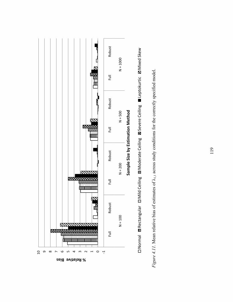
119

Fig

ure

4.1

1. M

ean r

elat

ive

bia

s of

esti

mat

es o

f λ

1,1 a

cross

stu

dy c

ondit

ions

for

the

corr

ectl

y s

pec

ifie

d m

odel

.

-10123456789

10

Fu

llR

ob

ust

Fu

llR

ob

ust

Fu

llR

ob

ust

Fu

llR

ob

ust

N =

10

0N

= 2

00

N =

50

0N

= 1

00

0

% Relative Bias

Sa

mp

le S

ize

by

Est

ima

tio

n M

eth

od

No

rma

lR

ect

an

gu

lar

Mil

d C

eil

ing

Mo

de

rate

Ce

ilin

gS

eve

re C

eil

ing

Lep

toku

rtic

Mix

ed

Ske

w

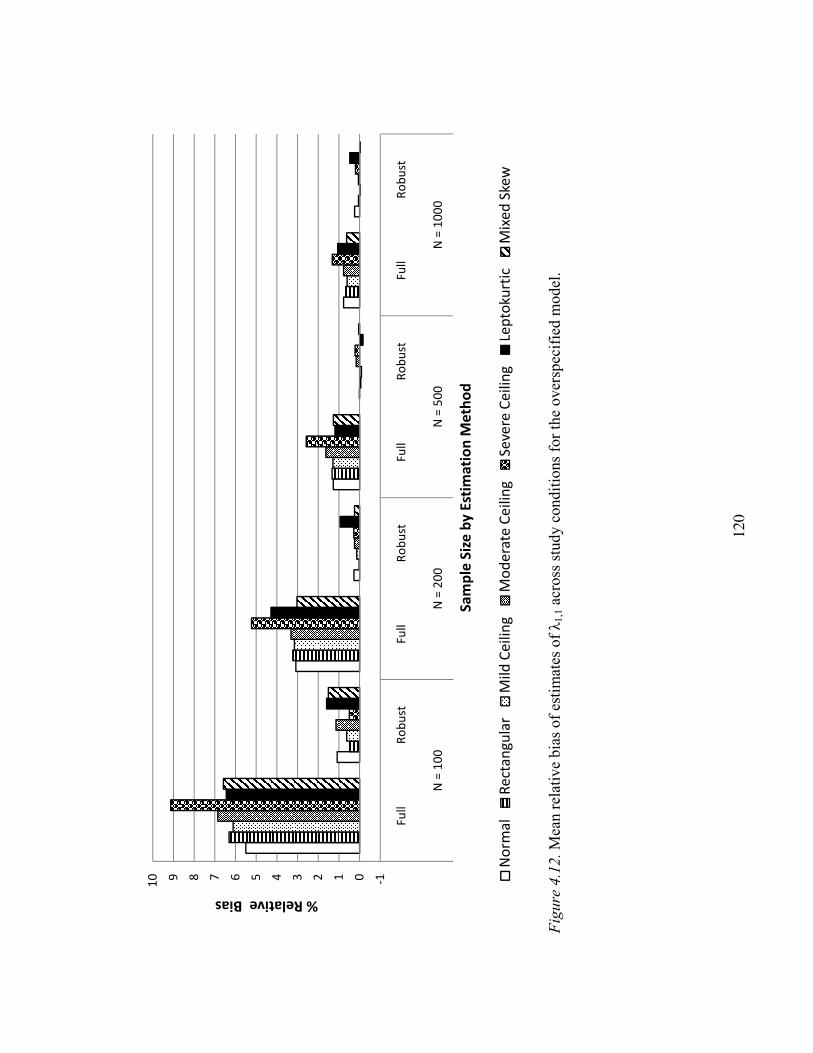
120

Fig

ure

4.1

2. M

ean r

elat

ive

bia

s of

esti

mat

es o

f λ

1,1 a

cross

stu

dy c

ondit

ions

for

the

over

spec

ifie

d m

odel

.

-10123456789

10

Fu

llR

ob

ust

Fu

llR

ob

ust

Fu

llR

ob

ust

Fu

llR

ob

ust

N =

10

0N

= 2

00

N =

50

0N

= 1

00

0

% Relative Bias

Sa

mp

le S

ize

by

Est

ima

tio

n M

eth

od

No

rma

lR

ect

an

gu

lar

Mil

d C

eil

ing

Mo

de

rate

Ce

ilin

gS

eve

re C

eil

ing

Lep

toku

rtic

Mix

ed

Ske

w

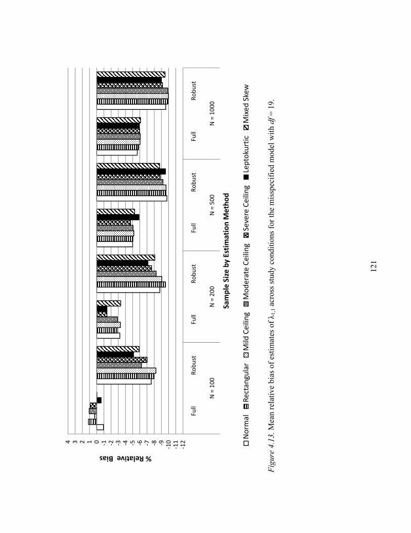
121

Fig

ure

4.1

3. M

ean r

elat

ive

bia

s of

esti

mat

es o

f λ

1,1 a

cross

stu

dy c

ondit

ions

for

the

mis

spec

ifie

d m

odel

wit

h d

f =

19.

-12

-11

-10-9-8-7-6-5-4-3-2-101234

Fu

llR

ob

ust

Fu

llR

ob

ust

Fu

llR

ob

ust

Fu

llR

ob

ust

N =

10

0N

= 2

00

N =

50

0N

= 1

00

0

% Relative Bias

Sa

mp

le S

ize

by

Est

ima

tio

n M

eth

od

No

rma

lR

ect

an

gu

lar

Mil

d C

eil

ing

Mo

de

rate

Ce

ilin

gS

eve

re C

eil

ing

Lep

toku

rtic

Mix

ed

Ske

w

122

Fig

ure

4.1

4. M

ean r

elat

ive

bia

s of

esti

mat

es o

f λ

1,1 a

cross

stu

dy c

ondit

ions

for

the

mis

spec

ifie

d m

odel

wit

h d

f =

17.

-12

-11

-10-9-8-7-6-5-4-3-2-101234

Fu

llR

ob

ust

Fu

llR

ob

ust

Fu

llR

ob

ust

Fu

llR

ob

ust

N =

10

0N

= 2

00

N =

50

0N

= 1

00

0

% Relative Bias

Sa

mp

le S

ize

by

Est

ima

tio

n M

eth

od

No

rma

lR

ect

an

gu

lar

Mil

d C

eil

ing

Mo

de

rate

Ce

ilin

gS

eve

re C

eil

ing

Lep

toku

rtic

Mix

ed

Ske

w

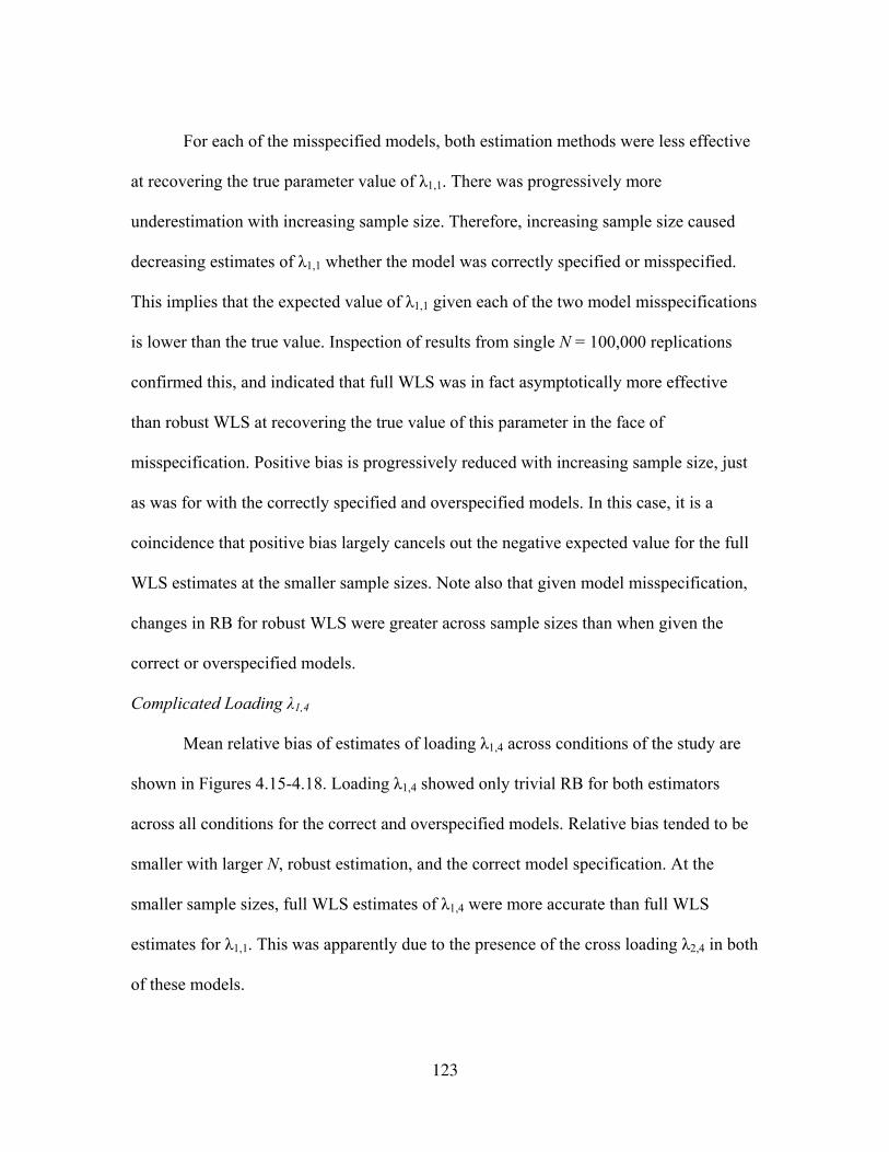
123

For each of the misspecified models, both estimation methods were less effective

at recovering the true parameter value of λ1,1. There was progressively more

underestimation with increasing sample size. Therefore, increasing sample size caused

decreasing estimates of λ1,1 whether the model was correctly specified or misspecified.

This implies that the expected value of λ1,1 given each of the two model misspecifications

is lower than the true value. Inspection of results from single N = 100,000 replications

confirmed this, and indicated that full WLS was in fact asymptotically more effective

than robust WLS at recovering the true value of this parameter in the face of

misspecification. Positive bias is progressively reduced with increasing sample size, just

as was for with the correctly specified and overspecified models. In this case, it is a

coincidence that positive bias largely cancels out the negative expected value for the full

WLS estimates at the smaller sample sizes. Note also that given model misspecification,

changes in RB for robust WLS were greater across sample sizes than when given the

correct or overspecified models.

Complicated Loading λ1,4

Mean relative bias of estimates of loading λ1,4 across conditions of the study are

shown in Figures 4.15-4.18. Loading λ1,4 showed only trivial RB for both estimators

across all conditions for the correct and overspecified models. Relative bias tended to be

smaller with larger N, robust estimation, and the correct model specification. At the

smaller sample sizes, full WLS estimates of λ1,4 were more accurate than full WLS

estimates for λ1,1. This was apparently due to the presence of the cross loading λ2,4 in both

of these models.

124

For each of the misspecified models, a large amount of overestimation was the

rule. This was due to the fact that this particular indicator variable measured both η1 and

η2 in the population model, but in each of the misspecifications the cross loading was

omitted. The estimators therefore generated higher estimates of λ1,4 to account for the

additional variance �� shared with η2. There was slightly less overestimation with the df

= 17 model, because the false cross loadings served as additional avenues through which

discrepancies between the initial polychoric correlation matrix and the reproduced matrix

could be reduced. Though the differences were small relative to the amount of overall

bias, bias increased with increasing N, and that bias was somewhat greater for robust

WLS. Inspection of N = 100,000 simulations confirmed that full WLS estimates were in

fact asymptotically more effective than robust estimates at recovering the true value of

this parameter in the face of misspecification. Note also that indicator distribution had a

greater effect at smaller N for both estimation methods with these misspecified models.

125

Fig

ure

4.1

5. M

ean r

elat

ive

bia

s of

esti

mat

es o

f λ

1,4 a

cross

stu

dy c

ondit

ions

for

the

corr

ectl

y s

pec

ifie

d m

odel

.

-1

-0.50

0.51

1.52

2.5

Fu

llR

ob

ust

Fu

llR

ob

ust

Fu

llR

ob

ust

Fu

llR

ob

ust

N =

10

0N

= 2

00

N =

50

0N

= 1

00

0

% Relative Bias

Sa

mp

le S

ize

by

Est

ima

tio

n M

eth

od

No

rma

lR

ect

an

gu

lar

Mil

d C

eil

ing

Mo

de

rate

Ce

ilin

gS

eve

re C

eil

ing

Lep

toku

rtic

Mix

ed

Ske

w

126

Fig

ure

4.1

6. M

ean r

elat

ive

bia

s of

esti

mat

es o

f λ

1,4 a

cross

stu

dy c

ondit

ions

for

the

over

spec

ifie

d m

odel

.

-1

-0.50

0.51

1.52

2.5

Fu

llR

ob

ust

Fu

llR

ob

ust

Fu

llR

ob

ust

Fu

llR

ob

ust

N =

10

0N

= 2

00

N =

50

0N

= 1

00

0

% Relative Bias

Sa

mp

le S

ize

by

Est

ima

tio

n M

eth

od

No

rma

lR

ect

an

gu

lar

Mil

d C

eil

ing

Mo

de

rate

Ce

ilin

gS

eve

re C

eil

ing

Lep

toku

rtic

Mix

ed

Ske

w

127

Fig

ure

4.1

7. M

ean r

elat

ive

bia

s of

esti

mat

es o

f λ

1,4 a

cross

stu

dy c

ondit

ions

for

the

mis

spec

ifie

d m

odel

wit

h d

f =

19.

05

10

15

20

25

30

35

40

Fu

llR

ob

ust

Fu

llR

ob

ust

Fu

llR

ob

ust

Fu

llR

ob

ust

N =

10

0N

= 2

00

N =

50

0N

= 1

00

0

% Relative Bias

Sa

mp

le S

ize

by

Est

ima

tio

n M

eth

od

No

rma

lR

ect

an

gu

lar

Mil

d C

eil

ing

Mo

de

rate

Ce

ilin

gS

eve

re C

eil

ing

Lep

toku

rtic

Mix

ed

Ske

w

128

Fig

ure

4.1

8. M

ean r

elat

ive

bia

s of

esti

mat

es o

f λ

1,4 a

cross

stu

dy c

ondit

ions

for

the

mis

spec

ifie

d m

odel

wit

h d

f =

17.

05

10

15

20

25

30

35

40

Fu

llR

ob

ust

Fu

llR

ob

ust

Fu

llR

ob

ust

Fu

llR

ob

ust

N =

10

0N

= 2

00

N =

50

0N

= 1

00

0

% Relative Bias

Sa

mp

le S

ize

by

Est

ima

tio

n M

eth

od

No

rma

lR

ect

an

gu

lar

Mil

d C

eil

ing

Mo

de

rate

Ce

ilin

gS

eve

re C

eil

ing

Lep

toku

rtic

Mix

ed

Ske

w

129

True Cross Loading λ1,5

Only the correctly specified and the overspecified model estimated the true cross

loadings λ1,5 and λ2,4. Figures 4.19 and 4.20 display the observed relative bias of

estimates of λ1,5 for these two model specifications. Although the absolute level of RB

was usually trivial, note that at the three larger sample sizes robust WLS estimates of λ1,5

tended to be roughly as biased or slightly more biased than the full WLS estimates.

Robust WLS bias was usually negative, whereas full WLS bias was usually positive.

130

Fig

ure

4.1

9. M

ean r

elat

ive

bia

s of

esti

mat

es o

f λ

1,5 a

cross

stu

dy c

ondit

ions

for

the

corr

ectl

y s

pec

ifie

d m

odel

.

-6-4-202468

Fu

llR

ob

ust

Fu

llR

ob

ust

Fu

llR

ob

ust

Fu

llR

ob

ust

N =

10

0N

= 2

00

N =

50

0N

= 1

00

0

% Relative Bias

Sa

mp

le S

ize

by

Est

ima

tio

n M

eth

od

No

rma

lR

ect

an

gu

lar

Mil

d C

eil

ing

Mo

de

rate

Ce

ilin

gS

eve

re C

eil

ing

Lep

toku

rtic

Mix

ed

Ske

w

131

Fig

ure

4.2

0. M

ean r

elat

ive

bia

s of

esti

mat

es o

f λ

1,5 a

cross

stu

dy c

ondit

ions

for

the

over

spec

ifie

d m

odel

.

-6-4-202468

Fu

llR

ob

ust

Fu

llR

ob

ust

Fu

llR

ob

ust

Fu

llR

ob

ust

N =

10

0N

= 2

00

N =

50

0N

= 1

00

0

% Relative Bias

Sa

mp

le S

ize

by

Est

ima

tio

n M

eth

od

No

rma

lR

ect

an

gu

lar

Mil

d C

eil

ing

Mo

de

rate

Ce

ilin

gS

eve

re C

eil

ing

Lep

toku

rtic

Mix

ed

Ske

w

132

Superfluous Cross Loading λ2,3

Only the overspecified model and the df = 17 misspecified model contained the

false crossloadings, λ1,6 and λ2,3. Figures 4.21 and 4.22 show mean estimates of λ2,3 for

each of these models, respectively. Because the true value of these paths was 0, a

consideration of relative bias for these estimates is not possible. However, note that for

the overspecified model robust WLS consistently estimated λ2,3 as more negative than

full WLS at any particular sample size. Both methods estimated negative values for this

path given the misspecification, but robust estimates were consistently lower (i.e., of

greater absolute value) than full WLS estimates.

133

Fig

ure

4.2

1. M

ean e

stim

ated

val

ue

of

λ2

,3 a

cross

stu

dy c

ondit

ions

for

the

over

spec

ifie

d m

odel

. N

ote

that

λ2

,3 =

0 i

n t

he

corr

ectl

y s

pec

ifie

d p

opula

tion m

odel

.

-0.0

10

0.0

1

0.0

2

0.0

3

0.0

4

0.0

5

Fu

llR

ob

ust

Fu

llR

ob

ust

Fu

llR

ob

ust

Fu

llR

ob

ust

N =

10

0N

= 2

00

N =

50

0N

= 1

00

0

Mean Loading Value

Sa

mp

le S

ize

by

Est

ima

tio

n M

eth

od

No

rma

lR

ect

an

gu

lar

Mil

d C

eil

ing

Mo

de

rate

Ce

ilin

gS

eve

re C

eil

ing

Lep

toku

rtic

Mix

ed

Ske

w

134

Fig

ure

4.2

2. M

ean e

stim

ated

val

ue

of

λ2

,3 a

cross

stu

dy c

ondit

ions

for

the

mis

spec

ifie

d m

odel

wit

h d

f =

17. N

ote

that

λ2

,3 =

0 i

n

the

corr

ectl

y s

pec

ifie

d p

opula

tion m

odel

.

-0.2

5

-0.2

-0.1

5

-0.1

-0.0

50

Fu

llR

ob

ust

Fu

llR

ob

ust

Fu

llR

ob

ust

Fu

llR

ob

ust

N =

10

0N

= 2

00

N =

50

0N

= 1

00

0

Mean Loading Value

Sa

mp

le S

ize

by

Est

ima

tio

n M

eth

od

No

rma

lR

ect

an

gu

lar

Mil

d C

eil

ing

Mo

de

rate

Ce

ilin

gS

eve

re C

eil

ing

Lep

toku

rtic

Mix

ed

Ske

w

135

Factor Correlation ψ

Mean relative bias of estimates of ψ is shown for each of the four model

specifications in Figures 4.23-4.26. When the model was correctly specified or

overspecified, robust WLS estimates of ψ showed bias near or below 5% across all

sample sizes and indicator distributions, with less bias at larger sample sizes. Full WLS

estimates of ψ for these two models were trivially biased at the sample sizes of 500 and

1000. At the two smaller sample sizes, full WLS estimates sometimes showed bias that

was moderate or substantial.

Note that robust estimates of ψ given the two misspecified models were largely

unaffected by both sample size and indicator distribution. Full WLS estimates of ψ

showed almost as little sensitivity to sample size, but somewhat more to indicator shape.

These estimates were usually more than 20% higher than robust estimates given the df =

17 misspecification and roughly 35% higher given the df = 19 misspecification. Much of

the positive bias present for both estimation methods with these models was clearly due

to the increased expected value of ψ given these misspecifications. The absence of the

true cross loadings resulted in increased estimated values of ψ in order to reconcile the

unmodeled covariance between η1 and ��, and also between η2 and ��

�.

136

Fig

ure

4.2

3. M

ean r

elat

ive

bia

s of

esti

mat

es o

f ψ

acr

oss

stu

dy c

ondit

ions

for

the

corr

ectl

y s

pec

ifie

d m

odel

.

-202468

10

12

14

16

Fu

llR

ob

ust

Fu

llR

ob

ust

Fu

llR

ob

ust

Fu

llR

ob

ust

N =

10

0N

= 2

00

N =

50

0N

= 1

00

0

% Relative Bias

Sa

mp

le S

ize

by

Est

ima

tio

n M

eth

od

No

rma

lR

ect

an

gu

lar

Mil

d C

eil

ing

Mo

de

rate

Ce

ilin

gS

eve

re C

eil

ing

Lep

toku

rtic

Mix

ed

Ske

w

137

Fig

ure

4.2

4. M

ean r

elat

ive

bia

s of

esti

mat

es o

f ψ

acr

oss

stu

dy c

ondit

ions

for

the

over

spec

ifie

d m

odel

.

-18

-16

-14

-12

-10-8-6-4-20246

Fu

llR

ob

ust

Fu

llR

ob

ust

Fu

llR

ob

ust

Fu

llR

ob

ust

N =

10

0N

= 2

00

N =

50

0N

= 1

00

0

% Relative Bias

Sa

mp

le S

ize

by

Est

ima

tio

n M

eth

od

No

rma

lR

ect

an

gu

lar

Mil

d C

eil

ing

Mo

de

rate

Ce

ilin

gS

eve

re C

eil

ing

Lep

toku

rtic

Mix

ed

Ske

w

138

Fig

ure

4.2

5. M

ean r

elat

ive

bia

s of

esti

mat

es o

f ψ

acr

oss

stu

dy c

ondit

ions

for

the

mis

spec

ifie

d m

od

el w

ith d

f =

19.

0

20

40

60

80

10

0

12

0

14

0

16

0

Fu

llR

ob

ust

Fu

llR

ob

ust

Fu

llR

ob

ust

Fu

llR

ob

ust

N =

10

0N

= 2

00

N =

50

0N

= 1

00

0

% Relative Bias

Sa

mp

le S

ize

by

Est

ima

tio

n M

eth

od

No

rma

lR

ect

an

gu

lar

Mil

d C

eil

ing

Mo

de

rate

Ce

ilin

gS

eve

re C

eil

ing

Lep

toku

rtic

Mix

ed

Ske

w

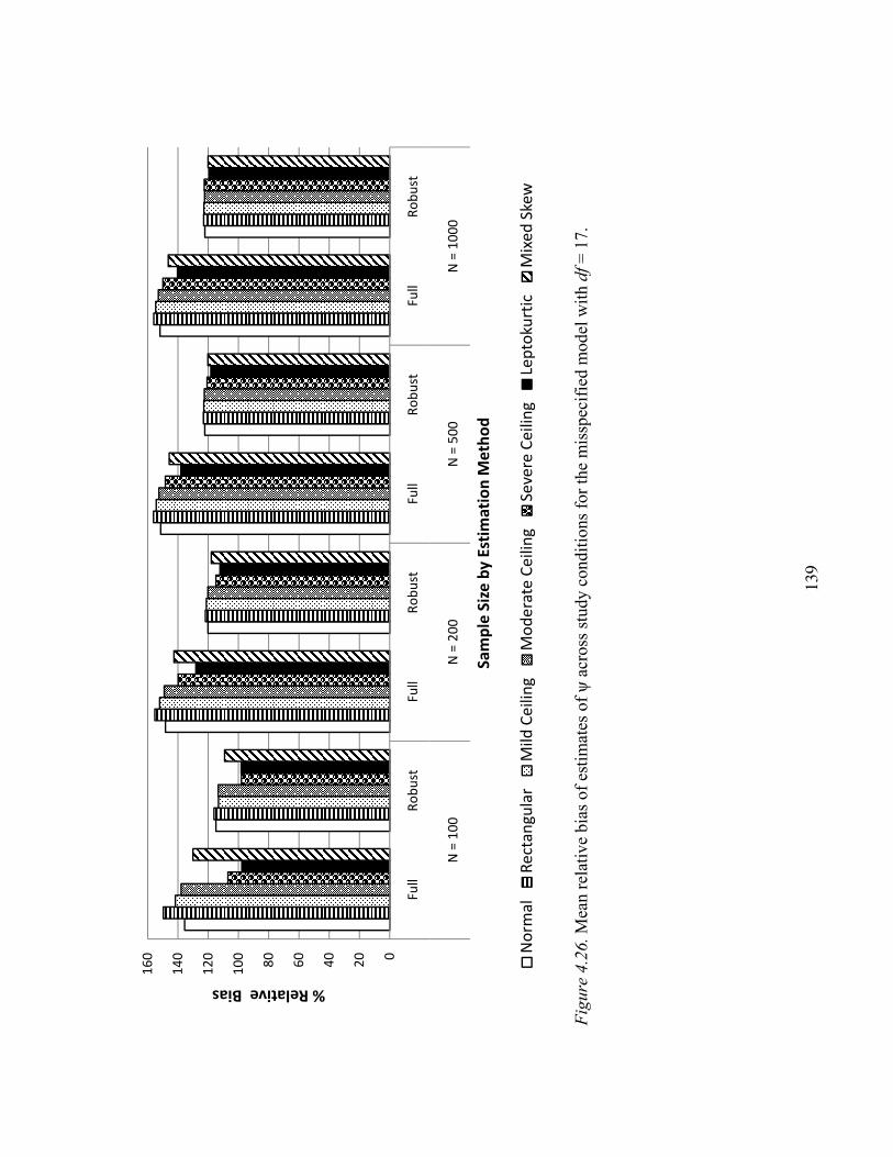
139

Fig

ure

4.2

6. M

ean r

elat

ive

bia

s of

esti

mat

es o

f ψ

acr

oss

stu

dy c

ondit

ions

for

the

mis

spec

ifie

d m

od

el w

ith d

f =

17.

0

20

40

60

80

10

0

12

0

14

0

16

0

Fu

llR

ob

ust

Fu

llR

ob

ust

Fu

llR

ob

ust

Fu

llR

ob

ust

N =

10

0N

= 2

00

N =

50

0N

= 1

00

0

% Relative Bias

Sa

mp

le S

ize

by

Est

ima

tio

n M

eth

od

No

rma

lR

ect

an

gu

lar

Mil

d C

eil

ing

Mo

de

rate

Ce

ilin

gS

eve

re C

eil

ing

Lep

toku

rtic

Mix

ed

Ske

w

140

Mean Absolute Value of Relative Bias for All Estimated Parameters

Figures 4.27-4.30 display mean averaged absolute values of RB for the factor

correlation and all estimated paths other than λ2,3 and λ1,6. Differences between the two

estimation methods for the correctly specified and overspecified models were generally

not large. Even when sample size equaled 100, differences between full and robust WLS

within any particular indicator distribution were less than 5% for these models. The most

peaked distributions, severe ceiling and leptokurtic, caused the most bias with these two

models. Also note that mean absolute relative bias was consistently greater than 5% for

these two models except when N equaled 1000.

Given either of the misspecified models, robust WLS showed a moderate

advantage in approximating the correct model parameter values at N = 100. However,

given the overall amount of inaccuracy for both methods with these misspecified models,

this is perhaps not particularly important. Figures 4.29 and 4.30 also show that there was

generally less variability across distributions under misspecification than given correct or

overspecification, and that both estimation methods were largely unaffected by indicator

distribution at larger N. Because of the patterns of RB observed for the individual

parameters, the mean absolute RB advantage of robust WLS for the misspecified models

is attributable to its superiority in recovering the factor correlation.

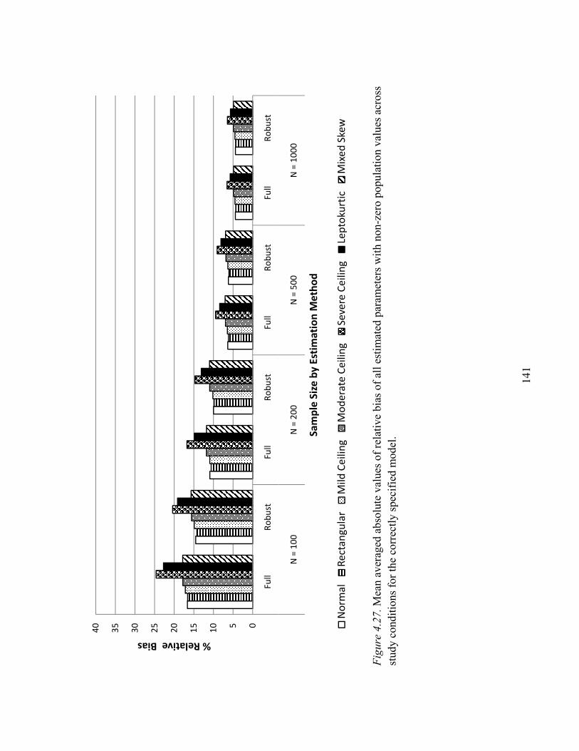
141

Fig

ure

4.2

7. M

ean a

ver

aged

abso

lute

val

ues

of

rela

tive

bia

s of

all

esti

mat

ed p

aram

eter

s w

ith n

on-z

ero p

opula

tion v

alues

acr

oss

study c

ondit

ions

for

the

corr

ectl

y s

pec

ifie

d m

od

el.

05

10

15

20

25

30

35

40

Fu

llR

ob

ust

Fu

llR

ob

ust

Fu

llR

ob

ust

Fu

llR

ob

ust

N =

10

0N

= 2

00

N =

50

0N

= 1

00

0

% Relative Bias

Sa

mp

le S

ize

by

Est

ima

tio

n M

eth

od

No

rma

lR

ect

an

gu

lar

Mil

d C

eil

ing

Mo

de

rate

Ce

ilin

gS

eve

re C

eil

ing

Lep

toku

rtic

Mix

ed

Ske

w

142

Fig

ure

4.2

8. M

ean a

ver

aged

abso

lute

val

ues

of

rela

tive

bia

s of

all

esti

mat

ed p

aram

eter

s w

ith n

on-z

ero p

opula

tion v

alues

acr

oss

study c

ondit

ions

for

the

over

spec

ifie

d m

odel

.

05

10

15

20

25

30

35

40

Fu

llR

ob

ust

Fu

llR

ob

ust

Fu

llR

ob

ust

Fu

llR

ob

ust

N =

10

0N

= 2

00

N =

50

0N

= 1

00

0

% Relative Bias

Sa

mp

le S

ize

by

Est

ima

tio

n M

eth

od

No

rma

lR

ect

an

gu

lar

Mil

d C

eil

ing

Mo

de

rate

Ce

ilin

gS

eve

re C

eil

ing

Lep

toku

rtic

Mix

ed

Ske

w

143

Fig

ure

4.2

9. M

ean a

ver

aged

abso

lute

val

ues

of

rela

tive

bia

s of

all

esti

mat

ed p

aram

eter

s w

ith n

on-z

ero p

opula

tion v

alues

acr

oss

study c

ondit

ions

for

the

mis

spec

ifie

d m

odel

wit

h d

f =

19.

05

10

15

20

25

30

35

40

Fu

llR

ob

ust

Fu

llR

ob

ust

Fu

llR

ob

ust

Fu

llR

ob

ust

N =

10

0N

= 2

00

N =

50

0N

= 1

00

0

% Relative Bias

Sa

mp

le S

ize

by

Est

ima

tio

n M

eth

od

No

rma

lR

ect

an

gu

lar

Mil

d C

eil

ing

Mo

de

rate

Ce

ilin

gS

eve

re C

eil

ing

Lep

toku

rtic

Mix

ed

Ske

w

144

Fig

ure

4.3

0. M

ean a

ver

aged

abso

lute

val

ues

of

rela

tive

bia

s of

all

esti

mat

ed p

aram

eter

s w

ith n

on-z

ero p

opula

tion v

alues

acr

oss

study c

ondit

ions

for

the

mis

spec

ifie

d m

odel

wit

h d

f =

17.

05

10

15

20

25

30

35

40

Fu

llR

ob

ust

Fu

llR

ob

ust

Fu

llR

ob

ust

Fu

llR

ob

ust

N =

10

0N

= 2

00

N =

50

0N

= 1

00

0

% Relative Bias

Sa

mp

le S

ize

by

Est

ima

tio

n M

eth

od

No

rma

lR

ect

an

gu

lar

Mil

d C

eil

ing

Mo

de

rate

Ce

ilin

gS

eve

re C

eil

ing

Lep

toku

rtic

Mix

ed

Ske

w

145

Precision of Parameter Estimates


The empirical standard deviations observed for λ1,1 within each combination of

indicator distribution, sample size, and estimation method are shown for each of the four

model specifications in figures 4.31-4.34. For each method, across all models and sample

sizes the leptokurtic and severe ceiling distributions caused more variability in the

estimates. This was most noticeable with smaller sample sizes. For the correct and

overspecified models at the sample size of 100, there was very little difference between

the two estimators except given the severe ceiling and leptokurtic distributions. At N =

500 and above, the two methods showed only very small differences across indicator

distributions. Differences between the estimators were more pronounced when models

were misspecified. Perhaps interestingly, this was mostly the result of full WLS estimates

of λ1,1 showing greater variability under these conditions; robust WLS variability

remained approximately the same as for the correct and overspecified models.

146

Fig

ure

4.3

1. W

ithin

-cel

l st

andar

d d

evia

tions

of

esti

mat

es o

f λ

1,1

acr

oss

stu

dy c

ondit

ions

for

the

corr

ectl

y s

pec

ifie

d m

odel

.

0

0.0

2

0.0

4

0.0

6

0.0

8

0.1

0.1

2

0.1

4

0.1

6

Fu

llR

ob

ust

Fu

llR

ob

ust

Fu

llR

ob

ust

Fu

llR

ob

ust

N =

10

0N

= 2

00

N =

50

0N

= 1

00

0

Within-Cell Standard Deviation

Sa

mp

le S

ize

by

Est

ima

tio

n M

eth

od

No

rma

lR

ect

an

gu

lar

Mil

d C

eil

ing

Mo

de

rate

Ce

ilin

gS

eve

re C

eil

ing

Lep

toku

rtic

Mix

ed

Ske

w

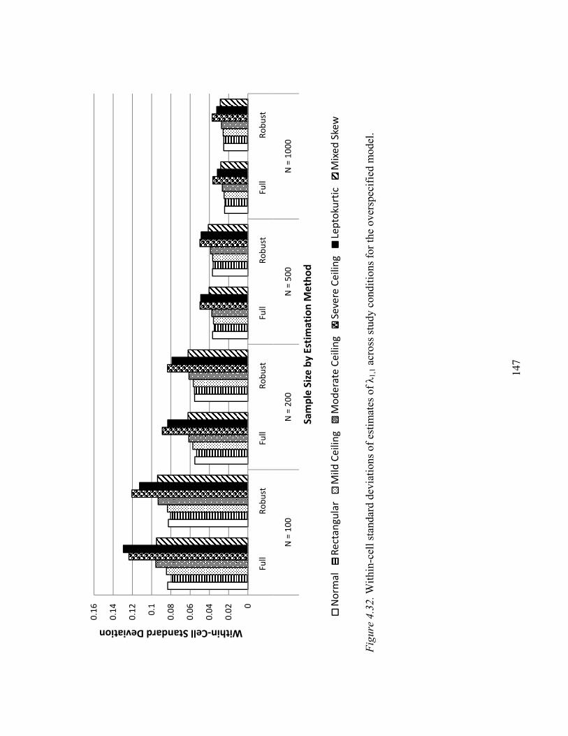
147

Fig

ure

4.3

2. W

ithin

-cel

l st

andar

d d

evia

tions

of

esti

mat

es o

f λ

1,1

acr

oss

stu

dy c

ondit

ions

for

the

over

spec

ifie

d m

odel

.

0

0.0

2

0.0

4

0.0

6

0.0

8

0.1

0.1

2

0.1

4

0.1

6

Fu

llR

ob

ust

Fu

llR

ob

ust

Fu

llR

ob

ust

Fu

llR

ob

ust

N =

10

0N

= 2

00

N =

50

0N

= 1

00

0


Sa

mp

le S

ize

by

Est

ima

tio

n M

eth

od

No

rma

lR

ect

an

gu

lar

Mil

d C

eil

ing

Mo

de

rate

Ce

ilin

gS

eve

re C

eil

ing

Lep

toku

rtic

Mix

ed

Ske

w

148

F

igure

4.3

3. W

ithin

-cel

l st

andar

d d

evia

tions

of

esti

mat

es o

f λ

1,1

acr

oss

stu

dy c

ondit

ions

for

the

mis

spec

ifie

d m

odel

wit

h d

f =

19.

0

0.0

2

0.0

4

0.0

6

0.0

8

0.1

0.1

2

0.1

4

0.1

6

Fu

llR

ob

ust

Fu

llR

ob

ust

Fu

llR

ob

ust

Fu

llR

ob

ust

N =

10

0N

= 2

00

N =

50

0N

= 1

00

0


Sa

mp

le S

ize

by

Est

ima

tio

n M

eth

od

No

rma

lR

ect

an

gu

lar

Mil

d C

eil

ing

Mo

de

rate

Ce

ilin

gS

eve

re C

eil

ing

Lep

toku

rtic

Mix

ed

Ske

w

149

Fig

ure

4.3

4. W

ithin

-cel

l st

andar

d d

evia

tions

of

esti

mat

es o

f λ

1,1

acr

oss

stu

dy c

ondit

ions

for

the

mis

spec

ifie

d m

odel

wit

h d

f =

17.

0

0.0

2

0.0

4

0.0

6

0.0

8

0.1

0.1

2

0.1

4

0.1

6

Fu

llR

ob

ust

Fu

llR

ob

ust

Fu

llR

ob

ust

Fu

llR

ob

ust

N =

10

0N

= 2

00

N =

50

0N

= 1

00

0


Sa

mp

le S

ize

by

Est

ima

tio

n M

eth

od

No

rma

lR

ect

an

gu

lar

Mil

d C

eil

ing

Mo

de

rate

Ce

ilin

gS

eve

re C

eil

ing

Lep

toku

rtic

Mix

ed

Ske

w

150


Figures 4.35-4.38 display variability in estimates of λ1,4 across the four model

specifications. When the model was correctly specified or overspecified, estimates of this

parameter generally showed the same patterns as were observed for λ1,1. That is, the only

notable between-method differences appeared at N = 100, and the two least normal

indicator distributions are the most problematic for each method.

Interestingly, overall variability in estimates of λ1,4 was clearly lower given model

misspecification. This lower variance was due to the fact that the estimates of this loading

were considerably overestimated relative to the population value of .70 (see Figures 4.17

and 4.18). Because all variances of factors and latent response variables were fixed at 1.0,

solutions with estimates of λ1,4 that are greater than 1.0 were rare and were among those

solutions removed as inadmissible. This resulted in a ceiling effect for estimates of λ1,4

for these misspecified models. Differences between full and robust WLS in the variability

of this parameter were negligible across all conditions for these misspecified models,

perhaps in part due to this restriction of range. This ceiling effect may also explain why

misspecification attenuated differences between the two estimation methods on this

outcome rather than enhanced them, as it has often been observed to do in the present

study. Many valid solutions estimated λ1,4 to be at or near 1.0 in value because of its role

in reconciling covariance between �� and η2.

151

Fig

ure

4.3

5. W

ithin

-cel

l st

andar

d d

evia

tions

of

esti

mat

es o

f λ

1,4

acr

oss

stu

dy c

ondit

ions

for

the

corr

ectl

y s

pec

ifie

d m

odel

.

0

0.0

2

0.0

4

0.0

6

0.0

8

0.1

0.1

2

0.1

4

0.1

6

Fu

llR

ob

ust

Fu

llR

ob

ust

Fu

llR

ob

ust

Fu

llR

ob

ust

N =

10

0N

= 2

00

N =

50

0N

= 1

00

0


Sa

mp

le S

ize

by

Est

ima

tio

n M

eth

od

No

rma

lR

ect

an

gu

lar

Mil

d C

eil

ing

Mo

de

rate

Ce

ilin

gS

eve

re C

eil

ing

Lep

toku

rtic

Mix

ed

Ske

w

152

Fig

ure

4.3

6. W

ithin

-cel

l st

andar

d d

evia

tions

of

esti

mat

es o

f λ

1,4

acr

oss

stu

dy c

ondit

ions

for

the

over

spec

ifie

d m

odel

.

0

0.0

2

0.0

4

0.0

6

0.0

8

0.1

0.1

2

0.1

4

0.1

6

Fu

llR

ob

ust

Fu

llR

ob

ust

Fu

llR

ob

ust

Fu

llR

ob

ust

N =

10

0N

= 2

00

N =

50

0N

= 1

00

0


Sa

mp

le S

ize

by

Est

ima

tio

n M

eth

od

No

rma

lR

ect

an

gu

lar

Mil

d C

eil

ing

Mo

de

rate

Ce

ilin

gS

eve

re C

eil

ing

Lep

toku

rtic

Mix

ed

Ske

w

153

Fig

ure

4.3

7. W

ithin

-cel

l st

andar

d d

evia

tions

of

esti

mat

es o

f λ

1,4

acr

oss

stu

dy c

ondit

ions

for

the

mis

spec

ifie

d m

odel

wit

h d

f =

19.

0

0.0

2

0.0

4

0.0

6

0.0

8

0.1

0.1

2

0.1

4

0.1

6

Fu

llR

ob

ust

Fu

llR

ob

ust

Fu

llR

ob

ust

Fu

llR

ob

ust

N =

10

0N

= 2

00

N =

50

0N

= 1

00

0


Sa

mp

le S

ize

by

Est

ima

tio

n M

eth

od

No

rma

lR

ect

an

gu

lar

Mil

d C

eil

ing

Mo

de

rate

Ce

ilin

gS

eve

re C

eil

ing

Lep

toku

rtic

Mix

ed

Ske

w

154

Fig

ure

4.3

8. W

ithin

-cel

l st

andar

d d

evia

tions

of

esti

mat

es o

f λ

1,4

acr

oss

stu

dy c

ondit

ions

for

the

mis

spec

ifie

d m

odel

wit

h d

f =

17.

0

0.0

2

0.0

4

0.0

6

0.0

8

0.1

0.1

2

0.1

4

0.1

6

Fu

llR

ob

ust

Fu

llR

ob

ust

Fu

llR

ob

ust

Fu

llR

ob

ust

N =

10

0N

= 2

00

N =

50

0N

= 1

00

0


Sa

mp

le S

ize

by

Est

ima

tio

n M

eth

od

No

rma

lR

ect

an

gu

lar

Mil

d C

eil

ing

Mo

de

rate

Ce

ilin

gS

eve

re C

eil

ing

Lep

toku

rtic

Mix

ed

Ske

w

155


The cross loading parameter λ1,5, which had a population value of .35, appeared

only in the correct and overspecified models. Observed variability in estimates of this

parameter for these models is displayed in Figures 4.39 and 4.40. As with the other

parameters, variability in estimates decreased with increasing N. For both estimation

methods there was somewhat more variability for the two most kurtotic distributions, and

this was especially true at smaller N. At the smaller sample sizes, full WLS estimates of

λ1,5 showed more variability that robust estimates. All of these patterns were somewhat

more noticeable for the overspecified model than the correctly specified model, and

variability in estimates of λ1,5 was slightly greater for the overspecified model.

156

Fig

ure

4.3

9. W

ithin

-cel

l st

andar

d d

evia

tions

of

esti

mat

es o

f λ

1,5

acr

oss

stu

dy c

ondit

ions

for

the

corr

ectl

y s

pec

ifie

d m

odel

.

0

0.0

2

0.0

4

0.0

6

0.0

8

0.1

0.1

2

0.1

4

0.1

6

0.1

8

0.2

Fu

llR

ob

ust

Fu

llR

ob

ust

Fu

llR

ob

ust

Fu

llR

ob

ust

N =

10

0N

= 2

00

N =

50

0N

= 1

00

0


Sa

mp

le S

ize

by

Est

ima

tio

n M

eth

od

No

rma

lR

ect

an

gu

lar

Mil

d C

eil

ing

Mo

de

rate

Ce

ilin

gS

eve

re C

eil

ing

Lep

toku

rtic

Mix

ed

Ske

w

157

Fig

ure

4.4

0. W

ithin

-cel

l st

andar

d d

evia

tions

of

esti

mat

es o

f λ

1,5

acr

oss

stu

dy c

ondit

ions

for

the

over

spec

ifie

d m

odel

.

0

0.0

2

0.0

4

0.0

6

0.0

8

0.1

0.1

2

0.1

4

0.1

6

0.1

8

0.2

Fu

llR

ob

ust

Fu

llR

ob

ust

Fu

llR

ob

ust

Fu

llR

ob

ust

N =

10

0N

= 2

00

N =

50

0N

= 1

00

0


Sa

mp

le S

ize

by

Est

ima

tio

n M

eth

od

No

rma

lR

ect

an

gu

lar

Mil

d C

eil

ing

Mo

de

rate

Ce

ilin

gS

eve

re C

eil

ing

Lep

toku

rtic

Mix

ed

Ske

w

158


Empirically observed standard deviations of estimates of λ2,3 for the overspecified

model and the misspecified model with 17 degrees of freedom are shown in Figures 4.41

and 4.42. For the overspecified model, variation in estimates of this false cross loading

decreased with increasing sample size, and was somewhat larger for the least normal

distributions. Relatively little difference between full and robust estimation was observed.

More overall variation in estimates of λ2,3 was observed for the misspecified model,

including larger differences between robust and full WLS estimation. With the

misspecified model, the severe ceiling distribution was seen to introduce disproportionate

variation into full WLS estimates at the two smaller sample sizes.

159

Fig

ure

4.4

1. W

ithin

-cel

l st

andar

d d

evia

tions

of

esti

mat

es o

f λ

2,3

acr

oss

stu

dy c

ondit

ions

for

the

over

spec

ifie

d m

odel

.

0

0.0

5

0.1

0.1

5

0.2

0.2

5

0.3

Fu

llR

ob

ust

Fu

llR

ob

ust

Fu

llR

ob

ust

Fu

llR

ob

ust

N =

10

0N

= 2

00

N =

50

0N

= 1

00

0


Sa

mp

le S

ize

by

Est

ima

tio

n M

eth

od

No

rma

lR

ect

an

gu

lar

Mil

d C

eil

ing

Mo

de

rate

Ce

ilin

gS

eve

re C

eil

ing

Lep

toku

rtic

Mix

ed

Ske

w

160

Fig

ure

4.4

2. W

ithin

-cel

l st

andar

d d

evia

tions

of

esti

mat

es o

f λ

2,3

acr

oss

stu

dy c

ondit

ions

for

the

mis

spec

ifie

d m

odel

wit

h d

f =

17.

0

0.0

5

0.1

0.1

5

0.2

0.2

5

0.3

Fu

llR

ob

ust

Fu

llR

ob

ust

Fu

llR

ob

ust

Fu

llR

ob

ust

N =

10

0N

= 2

00

N =

50

0N

= 1

00

0


Sa

mp

le S

ize

by

Est

ima

tio

n M

eth

od

No

rma

lR

ect

an

gu

lar

Mil

d C

eil

ing

Mo

de

rate

Ce

ilin

gS

eve

re C

eil

ing

Lep

toku

rtic

Mix

ed

Ske

w

161


Variation in estimates of ψ across the four models is displayed in Figures 4.43-

4.46. For the correctly specified and overspecified models, the pattern was largely

consistent with that observed for estimates of λ1,1 and λ1,4. Full WLS estimates showed

somewhat more variability than robust estimates at the smallest sample size. Variability

decreased with increasing sample size, and the severe ceiling and leptokurtic indicator

distributions caused the most variability in estimates for both methods. Differences in

variability caused by indicator distribution were most noticeable at the smallest sample

size.

There was less overall variation in estimates of ψ for the two incorrectly specified

models. Although the actual estimates of this parameter were inflated by around 100% in

even the best-performing conditions for these two models inspection of a histogram did

not reveal an obvious ceiling effect. As with other parameters, the two least normal

indicator distributions were associated with more variability in these estimates across all

four models.

162

Fig

ure

4.4

3. W

ithin

-cel

l st

andar

d d

evia

tions

of

esti

mat

es o

f ψ

acr

oss

stu

dy c

ondit

ions

for

the

corr

ectl

y s

pec

ifie

d m

odel

.

0

0.0

5

0.1

0.1

5

0.2

0.2

5

Fu

llR

ob

ust

Fu

llR

ob

ust

Fu

llR

ob

ust

Fu

llR

ob

ust

N =

10

0N

= 2

00

N =

50

0N

= 1

00

0


Sa

mp

le S

ize

by

Est

ima

tio

n M

eth

od

No

rma

lR

ect

an

gu

lar

Mil

d C

eil

ing

Mo

de

rate

Ce

ilin

gS

eve

re C

eil

ing

Lep

toku

rtic

Mix

ed

Ske

w

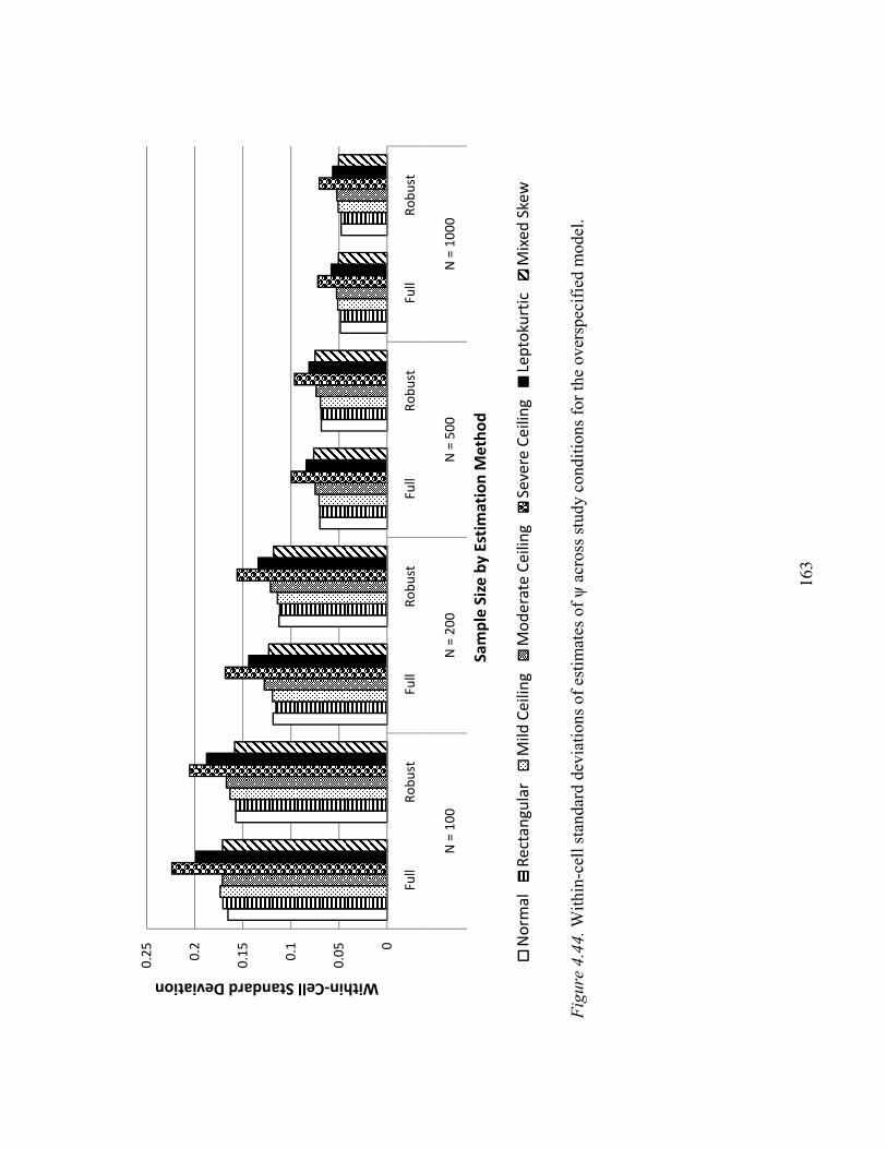
163

Fig

ure

4.4

4. W

ithin

-cel

l st

andar

d d

evia

tions

of

esti

mat

es o

f ψ

acr

oss

stu

dy c

ondit

ions

for

the

over

spec

ifie

d m

odel

.

0

0.0

5

0.1

0.1

5

0.2

0.2

5

Fu

llR

ob

ust

Fu

llR

ob

ust

Fu

llR

ob

ust

Fu

llR

ob

ust

N =

10

0N

= 2

00

N =

50

0N

= 1

00

0


Sa

mp

le S

ize

by

Est

ima

tio

n M

eth

od

No

rma

lR

ect

an

gu

lar

Mil

d C

eil

ing

Mo

de

rate

Ce

ilin

gS

eve

re C

eil

ing

Lep

toku

rtic

Mix

ed

Ske

w

164

Fig

ure

4.4

5. W

ithin

-cel

l st

andar

d d

evia

tions

of

esti

mat

es o

f ψ

acr

oss

stu

dy c

ondit

ions

for

the

mis

spec

ifie

d m

od

el w

ith d

f =

19.

0

0.0

5

0.1

0.1

5

0.2

0.2

5

Fu

llR

ob

ust

Fu

llR

ob

ust

Fu

llR

ob

ust

Fu

llR

ob

ust

N =

10

0N

= 2

00

N =

50

0N

= 1

00

0


Sa

mp

le S

ize

by

Est

ima

tio

n M

eth

od

No

rma

lR

ect

an

gu

lar

Mil

d C

eil

ing

Mo

de

rate

Ce

ilin

gS

eve

re C

eil

ing

Lep

toku

rtic

Mix

ed

Ske

w

165

Fig

ure

4.4

6. W

ithin

-cel

l st

andar

d d

evia

tions

of

esti

mat

es o

f ψ

acr

oss

stu

dy c

ondit

ions

for

the

mis

spec

ifie

d m

od

el w

ith d

f =

17.

0

0.0

5

0.1

0.1

5

0.2

0.2

5

Fu

llR

ob

ust

Fu

llR

ob

ust

Fu

llR

ob

ust

Fu

llR

ob

ust

N =

10

0N

= 2

00

N =

50

0N

= 1

00

0


Sa

mp

le S

ize

by

Est

ima

tio

n M

eth

od

No

rma

lR

ect

an

gu

lar

Mil

d C

eil

ing

Mo

de

rate

Ce

ilin

gS

eve

re C

eil

ing

Lep

toku

rtic

Mix

ed

Ske

w

166

Standard Errors of Parameter Estimates


Figures 4.47-4.50 show RB of the standard errors for estimates of λ1,1 supplied by

the two estimation methods for each of the four model specifications. For the correct and

overspecified models, robust estimates of standard errors clearly showed less bias at the

smaller sample sizes. At N = 500, all robust estimates were near or below the trivial

threshold, and all full WLS estimates were above this threshold. Robust estimates were

still generally smaller even at N = 1000, although full WLS estimates now showed less

than 5% RB except for the severe ceiling and mixed skew conditions.

Bias in standard errors of estimates of λ1,1 was worse for the two misspecified

models, although full WLS estimates clearly showed more of a decline in accuracy than

robust estimates. Full WLS standard errors were substantially biased at even the largest

sample size. And while the estimated SEs of both methods for the correct and

overspecified models appeared to suggest an asymptotic lack of bias or near lack of bias,

this was not obvious for the misspecified models.

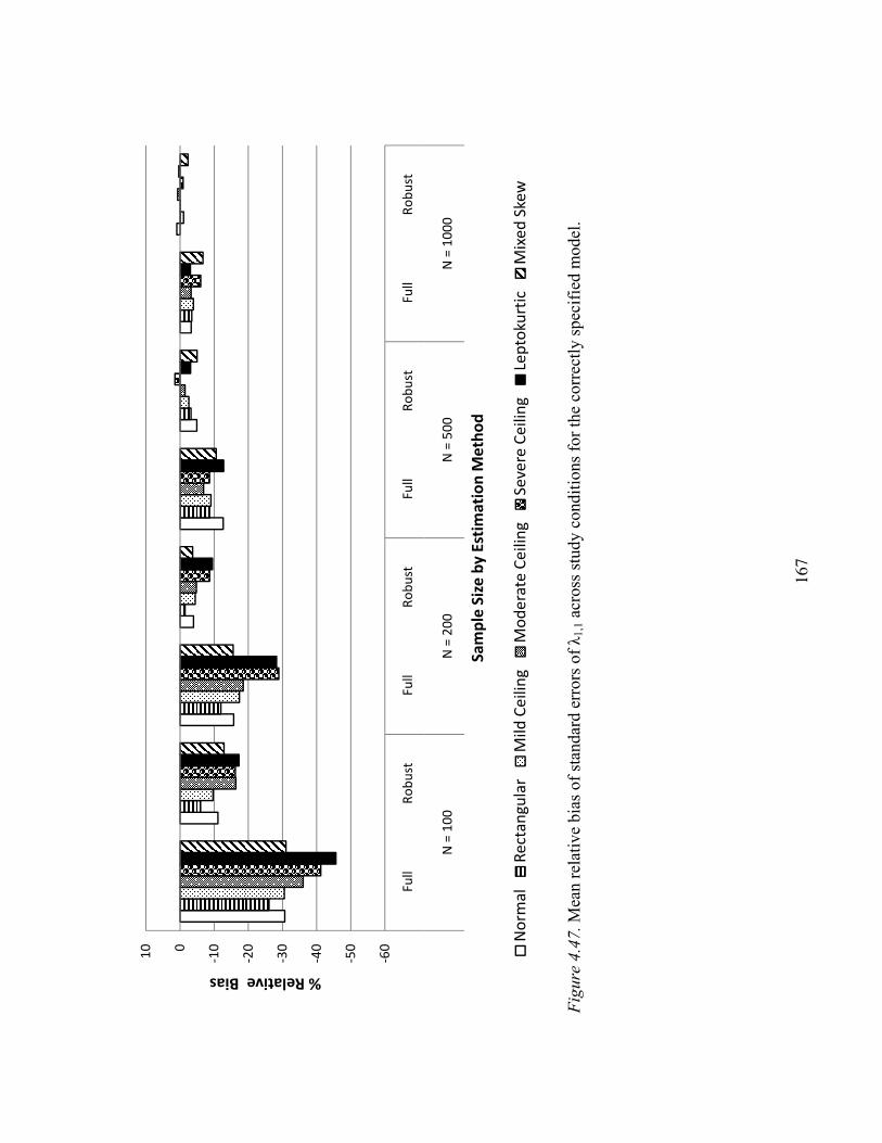
167

Fig

ure

4.4

7. M

ean r

elat

ive

bia

s of

stan

dar

d e

rrors

of

λ1

,1 a

cross

stu

dy c

ondit

ions

for

the

corr

ectl

y s

pec

ifie

d m

odel

.

-60

-50

-40

-30

-20

-100

10

Fu

llR

ob

ust

Fu

llR

ob

ust

Fu

llR

ob

ust

Fu

llR

ob

ust

N =

10

0N

= 2

00

N =

50

0N

= 1

00

0

% Relative Bias

Sa

mp

le S

ize

by

Est

ima

tio

n M

eth

od

No

rma

lR

ect

an

gu

lar

Mil

d C

eil

ing

Mo

de

rate

Ce

ilin

gS

eve

re C

eil

ing

Lep

toku

rtic

Mix

ed

Ske

w

168

Fig

ure

4.4

8. M

ean r

elat

ive

bia

s of

stan

dar

d e

rrors

of

λ1

,1 a

cross

stu

dy c

ondit

ions

for

the

over

spec

ifie

d m

odel

.

-60

-50

-40

-30

-20

-100

10

Fu

llR

ob

ust

Fu

llR

ob

ust

Fu

llR

ob

ust

Fu

llR

ob

ust

N =

10

0N

= 2

00

N =

50

0N

= 1

00

0

% Relative Bias

Sa

mp

le S

ize

by

Est

ima

tio

n M

eth

od

No

rma

lR

ect

an

gu

lar

Mil

d C

eil

ing

Mo

de

rate

Ce

ilin

gS

eve

re C

eil

ing

Lep

toku

rtic

Mix

ed

Ske

w

169

Fig

ure

4.4

9. M

ean r

elat

ive

bia

s of

stan

dar

d e

rrors

of

λ1

,1 a

cross

stu

dy c

ondit

ions

for

the

mis

spec

ifie

d m

odel

wit

h d

f =

19.

-60

-50

-40

-30

-20

-100

10

Fu

llR

ob

ust

Fu

llR

ob

ust

Fu

llR

ob

ust

Fu

llR

ob

ust

N =

10

0N

= 2

00

N =

50

0N

= 1

00

0

% Relative Bias

Sa

mp

le S

ize

by

Est

ima

tio

n M

eth

od

No

rma

lR

ect

an

gu

lar

Mil

d C

eil

ing

Mo

de

rate

Ce

ilin

gS

eve

re C

eil

ing

Lep

toku

rtic

Mix

ed

Ske

w

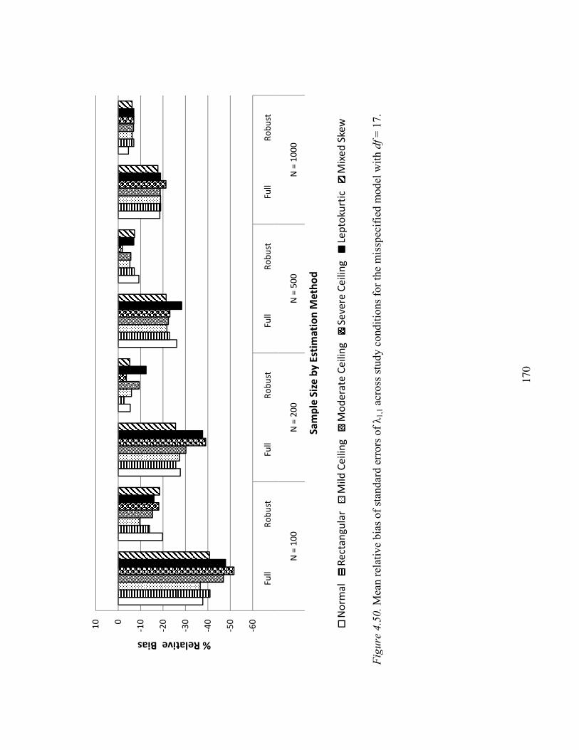
170

Fig

ure

4.5

0. M

ean r

elat

ive

bia

s of

stan

dar

d e

rrors

of

λ1

,1 a

cross

stu

dy c

ondit

ions

for

the

mis

spec

ifie

d m

odel

wit

h d

f =

17.

-60

-50

-40

-30

-20

-100

10

Fu

llR

ob

ust

Fu

llR

ob

ust

Fu

llR

ob

ust

Fu

llR

ob

ust

N =

10

0N

= 2

00

N =

50

0N

= 1

00

0

% Relative Bias

Sa

mp

le S

ize

by

Est

ima

tio

n M

eth

od

No

rma

lR

ect

an

gu

lar

Mil

d C

eil

ing

Mo

de

rate

Ce

ilin

gS

eve

re C

eil

ing

Lep

toku

rtic

Mix

ed

Ske

w

171


Relative biases of standard errors of estimates of λ1,4 across each of the four

modeling contexts are depicted in Figures 4.51-4.54. For the correctly specified and

overspecified models, robust WLS clearly outperformed full WLS, especially at smaller

sample sizes. Robust WLS estimates were relatively insensitive to sample size, in most

cases falling near or below the 5% cutoff for trivial bias. Bias in these estimated standard

errors tended to be negative rather than positive for both methods.

For the misspecified model with df = 19, robust WLS tended to substantially

overestimate standard errors, while full WLS underestimated them. Full WLS estimates

were generally more accurate than their robust counterparts, and sample size had little

effect on the accuracy of either method. For full WLS, the same pattern held for the

misspecified model with df = 17. For this model however, the estimated standard errors

provided by robust WLS did improve with increasing sample size. These robust

estimates showed trivial bias at N = 1000, surpassing the accuracy of full WLS estimates

at this sample size.

172

Fig

ure

4.5

1. M

ean r

elat

ive

bia

s of

stan

dar

d e

rrors

of

λ1

,4 a

cross

stu

dy c

ondit

ions

for

the

corr

ectl

y s

pec

ifie

d m

odel

.

-40

-30

-20

-100

10

20

30

40

Fu

llR

ob

ust

Fu

llR

ob

ust

Fu

llR

ob

ust

Fu

llR

ob

ust

N =

10

0N

= 2

00

N =

50

0N

= 1

00

0

% Relative Bias

Sa

mp

le S

ize

by

Est

ima

tio

n M

eth

od

No

rma

lR

ect

an

gu

lar

Mil

d C

eil

ing

Mo

de

rate

Ce

ilin

gS

eve

re C

eil

ing

Lep

toku

rtic

Mix

ed

Ske

w

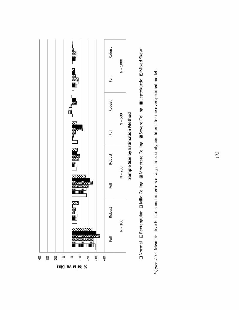
173

Fig

ure

4.5

2. M

ean r

elat

ive

bia

s of

stan

dar

d e

rrors

of

λ1

,4 a

cross

stu

dy c

ondit

ions

for

the

over

spec

ifie

d m

odel

.

-40

-30

-20

-100

10

20

30

40

Fu

llR

ob

ust

Fu

llR

ob

ust

Fu

llR

ob

ust

Fu

llR

ob

ust

N =

10

0N

= 2

00

N =

50

0N

= 1

00

0

% Relative Bias

Sa

mp

le S

ize

by

Est

ima

tio

n M

eth

od

No

rma

lR

ect

an

gu

lar

Mil

d C

eil

ing

Mo

de

rate

Ce

ilin

gS

eve

re C

eil

ing

Lep

toku

rtic

Mix

ed

Ske

w

174

Fig

ure

4.5

3. M

ean r

elat

ive

bia

s of

stan

dar

d e

rrors

of

λ1

,4 a

cross

stu

dy c

ondit

ions

for

the

mis

spec

ifie

d m

odel

wit

h d

f =

19.

-40

-30

-20

-100

10

20

30

40

Fu

llR

ob

ust

Fu

llR

ob

ust

Fu

llR

ob

ust

Fu

llR

ob

ust

N =

10

0N

= 2

00

N =

50

0N

= 1

00

0

% Relative Bias

Sa

mp

le S

ize

by

Est

ima

tio

n M

eth

od

No

rma

lR

ect

an

gu

lar

Mil

d C

eil

ing

Mo

de

rate

Ce

ilin

gS

eve

re C

eil

ing

Lep

toku

rtic

Mix

ed

Ske

w

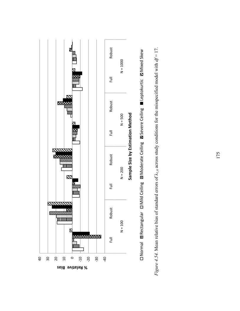
175

Fig

ure

4.5

4. M

ean r

elat

ive

bia

s of

stan

dar

d e

rrors

of

λ1

,4 a

cross

stu

dy c

ondit

ions

for

the

mis

spec

ifie

d m

odel

wit

h d

f =

17.

-40

-30

-20

-100

10

20

30

40

Fu

llR

ob

ust

Fu

llR

ob

ust

Fu

llR

ob

ust

Fu

llR

ob

ust

N =

10

0N

= 2

00

N =

50

0N

= 1

00

0

% Relative Bias

Sa

mp

le S

ize

by

Est

ima

tio

n M

eth

od

No

rma

lR

ect

an

gu

lar

Mil

d C

eil

ing

Mo

de

rate

Ce

ilin

gS

eve

re C

eil

ing

Lep

toku

rtic

Mix

ed

Ske

w

176


Relative biases of the standard errors of one of the true cross loadings, λ1,5, are

displayed in Figures 4.55 and 4.56 for the correctly specified and overspecified models,

respectively. The pattern of bias was roughly comparable for each model. Robust

standard errors were generally the most accurate, and were only trivially biased at the

sample sizes of 500 and 1000. Full WLS estimates were particularly inaccurate at smaller

sample sizes, and sometimes showed greater than trivial bias even at N = 1000. The two

least normal distributions, severe ceiling and leptokurtic, tended to cause the most bias.

This was especially true at smaller sample sizes and for full WLS.

177

Fig

ure

4.5

5. M

ean r

elat

ive

bia

s of

stan

dar

d e

rrors

of

λ1

,5 a

cross

stu

dy c

ondit

ions

for

the

corr

ectl

y s

pec

ifie

d m

odel

.

-45

-40

-35

-30

-25

-20

-15

-10-505

Fu

llR

ob

ust

Fu

llR

ob

ust

Fu

llR

ob

ust

Fu

llR

ob

ust

N =

10

0N

= 2

00

N =

50

0N

= 1

00

0

% Relative Bias

Sa

mp

le S

ize

by

Est

ima

tio

n M

eth

od

No

rma

lR

ect

an

gu

lar

Mil

d C

eil

ing

Mo

de

rate

Ce

ilin

gS

eve

re C

eil

ing

Lep

toku

rtic

Mix

ed

Ske

w

178

Fig

ure

4.5

6. M

ean r

elat

ive

bia

s of

stan

dar

d e

rrors

of

λ1

,5 a

cross

stu

dy c

ondit

ions

for

the

over

spec

ifie

d m

odel

.

-45

-40

-35

-30

-25

-20

-15

-10-505

Fu

llR

ob

ust

Fu

llR

ob

ust

Fu

llR

ob

ust

Fu

llR

ob

ust

N =

10

0N

= 2

00

N =

50

0N

= 1

00

0

% Relative Bias

Sa

mp

le S

ize

by

Est

ima

tio

n M

eth

od

No

rma

lR

ect

an

gu

lar

Mil

d C

eil

ing

Mo

de

rate

Ce

ilin

gS

eve

re C

eil

ing

Lep

toku

rtic

Mix

ed

Ske

w

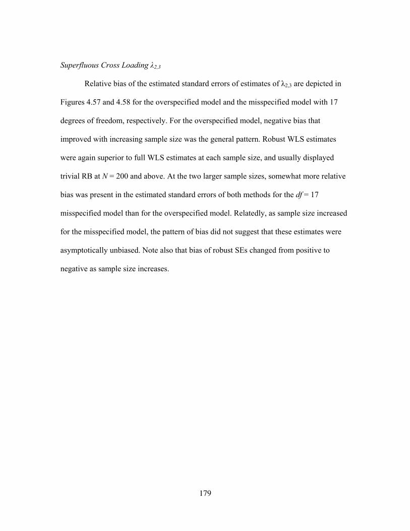
179


Relative bias of the estimated standard errors of estimates of λ2,3 are depicted in

Figures 4.57 and 4.58 for the overspecified model and the misspecified model with 17

degrees of freedom, respectively. For the overspecified model, negative bias that

improved with increasing sample size was the general pattern. Robust WLS estimates

were again superior to full WLS estimates at each sample size, and usually displayed

trivial RB at N = 200 and above. At the two larger sample sizes, somewhat more relative

bias was present in the estimated standard errors of both methods for the df = 17

misspecified model than for the overspecified model. Relatedly, as sample size increased

for the misspecified model, the pattern of bias did not suggest that these estimates were

asymptotically unbiased. Note also that bias of robust SEs changed from positive to

negative as sample size increases.

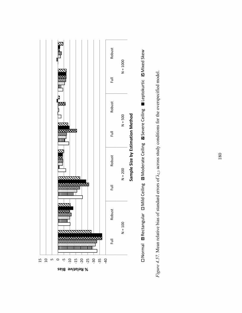
180

Fig

ure

4.5

7. M

ean r

elat

ive

bia

s of

stan

dar

d e

rrors

of

λ2

,3 a

cross

stu

dy c

ondit

ions

for

the

over

spec

ifie

d m

odel

.

-40

-35

-30

-25

-20

-15

-10-505

10

15

Fu

llR

ob

ust

Fu

llR

ob

ust

Fu

llR

ob

ust

Fu

llR

ob

ust

N =

10

0N

= 2

00

N =

50

0N

= 1

00

0

% Relative Bias

Sa

mp

le S

ize

by

Est

ima

tio

n M

eth

od

No

rma

lR

ect

an

gu

lar

Mil

d C

eil

ing

Mo

de

rate

Ce

ilin

gS

eve

re C

eil

ing

Lep

toku

rtic

Mix

ed

Ske

w

181

Fig

ure

4.5

8. M

ean r

elat

ive

bia

s of

stan

dar

d e

rrors

of

λ2

,3 a

cross

stu

dy c

ondit

ions

for

the

mis

spec

ifie

d m

odel

wit

h d

f =

17.

-40

-35

-30

-25

-20

-15

-10-505

10

15

Fu

llR

ob

ust

Fu

llR

ob

ust

Fu

llR

ob

ust

Fu

llR

ob

ust

N =

10

0N

= 2

00

N =

50

0N

= 1

00

0

% Relative Bias

Sa

mp

le S

ize

by

Est

ima

tio

n M

eth

od

No

rma

lR

ect

an

gu

lar

Mil

d C

eil

ing

Mo

de

rate

Ce

ilin

gS

eve

re C

eil

ing

Lep

toku

rtic

Mix

ed

Ske

w

182


Finally, figures 4.59-4.62 display the relative bias of standard error estimates for

ψ for each of the four model specifications. The correct and overspecified models showed

very similar patterns. Bias improved with increasing sample size for both methods, but

robust estimates consistently showed less bias at any particular sample size. For both

methods, estimates suggested asymptotic unbiasedness. At the smaller sample sizes, there

was slightly less bias for the overspecified model. The two must kurtotic distributions,

particularly the severe ceiling distribution, tended to be disproportionately troublesome

for full WLS. This was most notable at the smaller sample sizes.

Each misspecified model displayed a different pattern of bias. The df = 19

misspecified model was similar to the correctly specified model, except that overall

accuracy of estimated SEs was worse and the deleterious effects of the two most kurtotic

indicator distributions were amplified. Given the df = 17 misspecified model, robust

standard error estimates were near or below 5% absolute RB across all conditions except

the two most kurtotic distributions at N = 100. At sample sizes of 500 and 1000, full

WLS estimated SEs showed trivial RB except with the leptokurtic indicators. At the

sample sizes of 100 and 200, full WLS standard errors were generally more accurate than

given the previous three models, except for the leptokurtic and severe ceiling indicators.

183

Fig

ure

4.5

9. M

ean r

elat

ive

bia

s of

stan

dar

d e

rrors

of

ψ a

cross

stu

dy c

ondit

ions

for

the

corr

ectl

y s

pec

ifie

d m

od

el.

-70

-60

-50

-40

-30

-20

-100

10

Fu

llR

ob

ust

Fu

llR

ob

ust

Fu

llR

ob

ust

Fu

llR

ob

ust

N =

10

0N

= 2

00

N =

50

0N

= 1

00

0

% Relative Bias

Sa

mp

le S

ize

by

Est

ima

tio

n M

eth

od

No

rma

lR

ect

an

gu

lar

Mil

d C

eil

ing

Mo

de

rate

Ce

ilin

gS

eve

re C

eil

ing

Lep

toku

rtic

Mix

ed

Ske

w

184

Fig

ure

4.6

0. M

ean r

elat

ive

bia

s of

stan

dar

d e

rrors

of

ψ a

cross

stu

dy c

ondit

ions

for

the

over

spec

ifie

d m

odel

.

-70

-60

-50

-40

-30

-20

-100

10

Fu

llR

ob

ust

Fu

llR

ob

ust

Fu

llR

ob

ust

Fu

llR

ob

ust

N =

10

0N

= 2

00

N =

50

0N

= 1

00

0

% Relative Bias

Sa

mp

le S

ize

by

Est

ima

tio

n M

eth

od

No

rma

lR

ect

an

gu

lar

Mil

d C

eil

ing

Mo

de

rate

Ce

ilin

gS

eve

re C

eil

ing

Lep

toku

rtic

Mix

ed

Ske

w

185

Fig

ure

4.6

1. M

ean r

elat

ive

bia

s of

stan

dar

d e

rrors

of

ψ a

cross

stu

dy c

ondit

ions

for

the

mis

spec

ifie

d m

odel

wit

h d

f =

19.

-70

-60

-50

-40

-30

-20

-100

10

Fu

llR

ob

ust

Fu

llR

ob

ust

Fu

llR

ob

ust

Fu

llR

ob

ust

N =

10

0N

= 2

00

N =

50

0N

= 1

00

0

% Relative Bias

Sa

mp

le S

ize

by

Est

ima

tio

n M

eth

od

No

rma

lR

ect

an

gu

lar

Mil

d C

eil

ing

Mo

de

rate

Ce

ilin

gS

eve

re C

eil

ing

Lep

toku

rtic

Mix

ed

Ske

w

186

Fig

ure

4.6

2. M

ean r

elat

ive

bia

s of

stan

dar

d e

rrors

of

ψ a

cross

stu

dy c

ondit

ions

for

the

mis

spec

ifie

d m

odel

wit

h d

f =

17.

-70

-60

-50

-40

-30

-20

-100

10

Fu

llR

ob

ust

Fu

llR

ob

ust

Fu

llR

ob

ust

Fu

llR

ob

ust

N =

10

0N

= 2

00

N =

50

0N

= 1

00

0

% Relative Bias

Sa

mp

le S

ize

by

Est

ima

tio

n M

eth

od

No

rma

lR

ect

an

gu

lar

Mil

d C

eil

ing

Mo

de

rate

Ce

ilin

gS

eve

re C

eil

ing

Lep

toku

rtic

Mix

ed

Ske

w

187

Chapter V: Discussion

Full WLS and robust WLS are perhaps the only two potentially appropriate

estimators currently available for basic structural equation modeling applications

involving ordered categorical observed variables. Robust WLS had previously been

shown to outperform full WLS with correctly specified models (Flora & Curran, 2004;

Muthén, du Toit, & Spisic, 1997). A search of the literature revealed no studies that had

compared the performance of these estimators in the context of incorrectly specified

models. This study compared the performances of full WLS and robust WLS across

several conditions of sample size, distributional shape of indicators, and model

specification or misspecification. This chapter first summarizes and discusses the results,

relating them to prior research. Then, limitations of this study and avenues for future

work are discussed. Finally, recommendations are given for applied researchers.

Discussion and Summary of Results

Rates of Nonconvergence and Inadmissible Solutions

Given a significant model misspecification, failure to produce a valid solution

could perhaps be seen as a desirable property of an estimator. In general, nonconvergence

and invalid solutions were strongly indicative of model misspecification in the present

study. This was particularly true for robust WLS. The finding that robust WLS was less

likely than full WLS to produce and admissible solution given the df = 19 misspecified

model, yet often more likely to do so given the df = 17 model, was unexpected. The df =

19 misspecified model obviously entailed two fewer avenues for reconciling the sample

188

polychoric correlation matrix with the reproduced version. It is also interesting to note

that rates of valid solutions for both estimation methods were lower for the overspecified

model than for the correctly specified model. The causes of each of these patterns remain

unknown.

Expected Values of the Full WLS Chi-Square

The method described in Curran, West, and Finch (1996) was used to generate

expected values of the full WLS chi-square for the two misspecified models across

conditions of sample size and indicator distribution. The fact that the model degrees of

freedom were reproduced for the correctly specified and overspecified models indicated

that the method was appropriate for this context and was applied correctly. Recall that

Curran et al. examined continuous factor indicators with three different distributions. The

most marked distinction among these three distributions was positive kurtosis; one

distribution was normal, another had a skewness of 2.0 and a kurtosis of 7.0, and the third

indicator distribution had a skewness of 3.0 and a kurtosis of 21.0. Curran et al. found

that the expected values of the ADF chi-square decreased with increasing nonnormality,

suggesting decreased power to reject misspecified models. Because ADF and full WLS

each share the weakness of a large, unstable weight matrix, it is not surprising that the

present study found that full WLS expected values of chi-square also decreased with

increasing nonnormality. However, the present study showed that positive kurtosis

specifically was the most significant driver of low expected values. The lowest expected

values were observed with the severe ceiling and leptokurtic distributions, and the

189

decidedly nonnormal rectangular distribution actually showed the highest expected

values.

Performance of Chi-Square Statistics

This study largely replicated previous findings of excessive positive bias of the

full WLS chi-square for correctly specified models (Dolan, 1994; Potthast, 1993; Flora &

Curran, 2004). It is important to note that just as in Curran, West, and Finch (1996), the

overspecified model is essentially correctly specified in that it is expected on average to

correctly reproduce the input correlation matrix. A sample size of 500 was required for

marginally acceptable performance of the full WLS chi-square given the correct and

overspecified models. Performance of the full WLS chi-square with the two least normal

indicator distributions was still arguably inadequate at this sample size, in that rejection

rates were roughly three times greater than the expected rate of .01.

Recall that Potthast (1993) had examined full WLS with correctly specified

models at sample sizes of 500 and 1000. Her two factor model with 19 degrees of

freedom resembled the correctly specified models examined in the present study,

although it did not include cross loadings. At the sample size of 500, she found

acceptable performance of chi-square statistics for this model with the normal indicators.

With the negative kurtosis indicators, however, she found greater than 5% positive chi-

square bias. She found greater than 15% positive bias for each of the two positive

kurtosis conditions for this model at this sample size. For the same model at N = 1000,

she found chi-square to be inflated less than 5% for the negative kurtosis and normal

distribution indicators, but still moderately and substantially inflated with the positive

190

kurtosis and positive-kurtosis-and-skewed conditions, respectively. These patterns largely

match findings of the present study for the correct and overspecified models, though bias

was generally slightly lower in the present context. Performance was arguably acceptable

at N = 500 for the less kurtotic distributions. This is perhaps due to the presence of cross

loadings in the population model here utilized.

In his study of single-factor models, Dolan (1994) found the full WLS chi-square

to perform adequately at sample sizes of 300 and 400, with rejection rates close to the

expected 5% frequency. He found rejection rates to be too high at the sample size of 200.

Given the correct and overspecified models, the present study also found rejection rates

for the full WLS chi-square to be too high for all distributions of observed variables at the

sample size of 200. This was especially true for the severe ceiling and leptokurtic

distributions. The levels of nonnormality used by Dolan were milder than those of the

present study. Dolan used a simpler model however, although he also included conditions

with fewer than five categories of the ordinal indicators. Dolan’s use of the single-factor

model might explain why he found performance to be adequate at sample sizes of 300

and 400 while the present study found the full WLS chi-square to be arguably lacking at

N = 500.

DiStefano (2002), who used sample sizes of 350 and 700, had also found the full

WLS chi-square to be substantially positively biased with correctly specified models.

Nonnormal indicator distributions and smaller sample size increased bias, as in the

present study. The bias of the full WLS chi-square observed by DiStefano was perhaps

larger than would be expected based on the results of the present study. This is likely

191

attributable to the fact that DiStefano was reporting results for a three-factor model with

101 degrees of freedom; Dolan (1994), Potthast (1993), and Flora and Curran (2004)

found bias in this statistic to increase with increasing model size.

The previous studies revealed by the literature search did not include misspecified

models. The present study found that full WLS chi-squares showed similar patterns of

positive bias whether the model specification was correct or not. There was more bias

with increasing indicator kurtosis, and less bias with increasing sample size. The present

study used large sample estimates to produce expected chi-square values for full WLS

that also served as benchmarks for robust WLS. In principle, separate expected values

could have been produced for robust WLS by performing analogous large sample

estimations. The resulting robust WLS chi-square values could then be similarly

decomposed (see Equation 2.25) and rescaled according to sample size. The same chi-

square scaling procedure that was used to place robust chi-square estimates on par with

full WLS estimates for the purposes of calculating relative bias could then be applied as

necessary. This endeavor was not undertaken for three reasons. First, it was unknown

whether the more complex robust WLS fit function and associated chi-square mean- and

variance-adjustment was amenable to this scaling procedure. Second, Mplus simply did

not output a chi-square value for misspecified models estimated with robust WLS (known

as the WLSMV estimator in Mplus syntax) when N was extremely large. Third, the major

purpose of the study was to compare the performance of full WLS with that of robust

WLS. The use of a single standard for both methods is an effective way to evaluate their

relative performances.

192

Robust WLS showed far less positive bias than full WLS for correctly specified

and overspecified models in the present study. Robust WLS chi-squares were arguably

acceptable for these models even at the sample size of 100. At this sample size,

somewhat more bias was present for the indicator distributions with the most skew,

severe ceiling, moderate ceiling, and mixed skew. This observed superiority of robust

WLS chi-squares to those of full WLS given correctly specified models is consistent with

the results of Flora and Curran (2004) and the reports of Muthén, du Toit, and Spisic

(1997). However, the fact that the robust WLS chi-square exhibits any positive bias at all

for correctly specified models might add some support to the popular contention that the

chi-square test is generally too stringent a criterion for the evaluation of model fit.

Nevertheless, note the perhaps surprising lack of power of both estimation methods to

reject the two misspecified models at N = 200 given the 2 most peaked distributions (see

Figures 4.9 and 4.10).

For these misspecified models, the robust WLS chi-square demonstrated the

presumably desirable property of showing increasing observed values relative to full

WLS as sample size increased. That is, whereas positive bias in the full WLS chi-square

decreased with increasing sample size, robust WLS accrued more power to reject

misspecified models. Strictly speaking, these increasing values of chi-square are not

increasing bias per se for the robust method, because the expected values were

determined according to the full WLS large sample approximation. It is instead indicative

of the increasing power of robust WLS relative to full WLS with increasing sample size.

Because robust WLS also shows less positive bias at smaller sample sizes for correctly

193

specified models, this method appears to be generally better able to distinguish between

correct and misspecified models than the full WLS chi-square.

It is interesting to note that whereas the full WLS chi-squares show the most

positive bias for the severe ceiling and leptokurtic distributions regardless of model

specification, the robust chi-square values tend to be lowest for these two distributions

given model misspecification. This probably is caused by the Satorra-Bentler-type

scaling correction of robust WLS. As discussed by Curran, West, and Finch (1996),

scaling procedures of this type use some of the total available information in the data to

account for nonnormality. The tradeoff is that less total information is available for

detecting misspecification. This appears to be a worthwhile tradeoff in this context, given

the clearly inadequate performance of the full WLS chi-square. The large weight matrix

of full WLS is also supposed to trade power to detect misspecification for the ability to

account for nonnormality of the data. This is what was observed in Curran et al. for the

expected values of the ADF estimator, which shares with full WLS the large weight

matrix. By the standard of the calculated expected values, the full WLS estimator did

perform this tradeoff in the present study; for the two most kurtotic distributions,

expected values were lower. This lowering of expected values was not very noticeable at

the sample sizes of 100 and 200, however, and it was at these smaller sample sizes that

positive bias was most pronounced for the two distributions. Therefore, the full WLS

weight matrix is fundamentally inefficient, particularly at disentangling positive kurtosis

from misspecification.

194

As discussed in chapter II, Green, Akey, Fleming, Hershberger, and Marquis

(1997) found that the benefits of Satorra-Bentler scaling disappeared when factor

indicators were of opposite skew. Though Green et al. were applying ML estimation with

S-B scaling to ordered categorical data, this nevertheless suggested possible difficulties

for robust WLS when given mixed skew indicators. This is because the robust WLS

scaling correction is similar to the S-B correction. However, the present study found no

particular performance problem for the robust WLS chi-square with mixed skew

indicators in any condition.

Relative Bias of Parameter Estimates

Loading λ1,1 served as the representative example of the uncomplicated loadings

of any particular model specification. Here uncomplicated means that no other loading

applied to the same indicator in either the population model or the particular model

specified. Loadings like these are the most comparable with loadings from prior research

on full WLS, because cross loadings did not generally appear in that research. Findings

from the present study regarding estimates of λ1,1 largely replicated prior findings for full

WLS with correctly specified models. For example, Potthast (1993) found bias in

loadings was positive for full WLS, but less than 5% and not related to study conditions.

The smallest sample size used by Potthast was 500, and this is therefore entirely

consistent with the present research. When sample size was 500 and models were

correctly specified or overspecified in the present study, relative bias of estimates of λ1,1

was less than 3% across all indicator distributions. At sample sizes as small as 200, Dolan

(1994) found loading bias of both versions of full WLS to be positive but never greater

195

than 10% in any condition. Similarly, DiStefano (2002) found full WLS loadings to be

positively biased, but never greater than 8% in any condition. Even at N =100, the present

research never found the relative bias of λ1,1 to be greater than 9% for the correct and

overspecified models.

Consistent with prior research (Flora & Curran, 2004; Muthén, du Toit, & Spisic,

1997), robust estimates of λ1,1 showed very little bias for the correct and overspecified

models, in fact lower than 1.5% for all distributions at even the smallest sample size of

100. This is interesting because robust WLS makes use of less total information than full

WLS. Muthén’s (1993; Muthén et al., 1997) method of simply setting all off-diagonal

elements of the weight matrix to zero might seem to be a heavy handed approach.

Clearly, however, this method works well under these circumstances. The original off-

diagonal elements of WFull are apparently so unstable that it is best to dispense with them

completely.

For both full and robust WLS, relative bias in estimates of λ1,4 for the correctly

specified and overspecified models and relative bias in estimates of λ1,5, which only

appears in these models, was consistently within the trivial range. Though not practically

significant, it is perhaps surprising that full WLS consistently performs slightly better

than robust WLS for the cross loading, λ1,5. Accuracy for both methods probably results

substantially from the fact that λ1,5 is a cross loading, and the main loading for �� is

substantial in size.

Given the correct or overspecified model, the present research found more bias in

full WLS estimates of the factor correlation ψ than for estimates of λ1,1. This is consistent

196

with the findings of Potthast (1993) and DiStefano (2002), who each also found greater

bias for factor correlations than for loadings. Dolan considered only single factor models,

and so factor correlations were inapplicable. The present research found a similar pattern

for robust WLS. Though bias of these two parameters for these two models was in the

trivial range in all cases, bias in estimates of ψ was greater than bias in estimates of λ1,1 at

every sample size.

When models are misspecified, bias of parameter estimates becomes a more

complicated issue. Because the population value of the parameter for the correctly

specified model is used as the expected value, i.e. as θ in Equation 3.1, observed bias

given a misspecified model is the result of two separate influences. First, the asymptotic

value of the parameter may be different than the original θ that applies to the correctly

specified model. That is, regardless of the estimation method employed, the value of θ

that on average optimizes reproduction of the input matrix given misspecification may be

different than the original θ in the correctly specified model. Second, bias of the estimator

may perturb estimates of this new θ in the same general fashion that bias perturbed

estimates for correctly specified models. Alternatively, the nature of this perturbation

may be different for a misspecified model than it was for the correctly specified model.

When considering bias of parameter estimates for misspecified models, the present study

continued to use values of θ drawn from the correctly specified model as the standard of

comparison. This is because interest is generally in recovery of these values rather than

recovery of the asymptotic values of parameter estimates for incorrectly specified

197

models. Nevertheless, both influences on the bias of parameter estimates for misspecified

models must be considered when evaluating these estimates.

For either misspecified model, mean estimates of λ1,1 for both methods across all

distributions decreased with increasing sample size, incurring progressively more

negative bias. This is because the asymptotic value of λ1,1 was lower for these

misspecified models than for the correctly specified model. Both methods appeared to

show some leveling off of this negative bias, suggesting that further increases in sample

size would not have resulted in substantially lower estimates. It thus appeared that given

these two model misspecifications, full WLS estimates of this class of uncomplicated

loadings were closer to the correct values at small sample sizes as well as asymptotically.

This is perhaps practically significant in that the full WLS approximations of this loading

showed slightly more than trivial bias at the worst, whereas robust approximations were

often more than 5% worse than full WLS estimates.

Substantial overestimation of λ1,4 for both misspecified models was the rule for

both methods across all distributions. There was relatively little variation across method,

distribution, and sample size. This was because of the ceiling effect for estimates of this

loading. Estimates were constrained to be at or below 1.0, but very high values of this

loading were on average more effective for replicating the input polychoric correlation

matrix given these models. That is, given these misspecifications, the value of λ1,4 is

asymptotically higher than .70, the population value of interest. There was therefore

relatively little room for variation. Nevertheless, robust estimation consistently

demonstrated somewhat greater positive bias than full WLS estimation as sample size

198

increased. As with λ1,1, full WLS estimates seemed to be asymptotically closer to the

actual population value than those of robust WLS.

The parameter λ2,3 is a false cross loading, in that its true value is zero when the

model is correctly specified or overspecified. Given overspecification, both methods

estimated λ2,3 as near zero except when full WLS was used at the sample size of 100 with

the more skewed and/or kurtotic indicators. For both estimation methods, mean estimates

of λ2,3 given the misspecified model were substantially more negative and also larger in

absolute value. Due to the absence of the true cross loading, the expected value of this

parameter is less than zero. Increasing sample size showed that the estimates appeared to

stabilize for both methods at N = 1000, with robust WLS showing consistently more

negative bias across all indicator distributions. In the context of model misspecification,

robust WLS was more susceptible to foisting variance onto this parameter.

On the whole then, the advantages demonstrated by robust WLS for accuracy in

the estimation of loadings for correctly specified models were observed to reverse when

models were misspecified. Full WLS more effectively approximated the true parameters

in the face of misspecification at small sample sizes and was also more accurate

asymptotically. However, a different pattern was observed for estimates of ψ given

misspecification. While inflation was always very near 120% for robust WLS estimates,

full WLS consistently showed roughly 140-160% inflation in estimates of this parameter.

Indicator distribution generally had very little effect on either method, and bias changed

very little with increases in sample size. In this particular context of misspecification,

199

disposal of the off-diagonal of the full weight matrix seems to result in more accurate

approximation of correct factor correlations, but less accurate approximation of loadings.

In summary, the present research replicated previous research by showing that full

WLS trivially to moderately overestimates factor loadings for correctly specified models

when sample size is not large. Also as in prior research, slightly more overestimation was

observed for full WLS estimates of factor correlations for these models. Robust WLS

showed less bias for both types of parameters, just as Muthén, du Toit, and Spisic (1997)

and Flora and Curran (2004) reported. For misspecified models, a different pattern

emerged. For factor loadings, full WLS more effectively recovered values from the

correctly specified model in the face of misspecification. Bias for both methods was low

enough that this difference might be practically significant. For the factor correlation

however, robust WLS consistently showed less inflation. This difference in performance

might be less practically relevant, in that bias even for the robust estimates was around

+120%.

The mean absolute value of RB of all the estimated parameters for a particular

model specification with non-zero values in the population was calculated in an attempt

to provide an omnibus index of parameter estimate error in a meaningful metric. These

values included all estimated loadings other than the false cross loadings, as well as the

factor correlation. For example, absolute values of RB of estimates of λ1,1 λ1,2 λ1,3 λ1,4 λ1,5

λ2,4 λ2,5 λ2,6 λ2,7 λ2,8 and ψ were average to create this index for each repetition in which

the model was correctly specified or overspecified. Resulting values sometimes appeared

to be clearly higher than one would expect based on inspection of the RB of each of the

200

constituent parameters. This phenomenon results from the fact that, within any particular

set of parameter estimates, some of these estimates might in fact be negative. When this

is the case, the mean absolute value will be higher than the absolute value of the mean.

Mean values of RB rather than absolute values of RB have heretofore been presented in

order to preserve locational information about the bias of each parameter.

These mean absolute values of RB indicated that robust WLS had a slight overall

accuracy advantage for the correctly specified and overspecified models at the two

smaller sample sizes, and that accuracy was somewhat worse for both methods given the

two most kurtotic distributions. The previously discussed results indicate that it was

clearly the loadings rather than the factor correlations that drove this latter phenomenon.

At sample sizes of 500 and 1000 there was little difference between the two methods, and

the influence of the severe ceiling and leptokurtic distributions was not as great. Notably,

for either method this overall mean RB dipped below the 5% trivial bias threshold for

some distributions only when sample size equaled 1000 and the model was correctly

specified or overspecified. For this particular omnibus metric then, the robust WLS

advantage in estimating ψ for the misspecified models outweighed its disadvantages in

estimating the factor loadings. The overall level of inaccuracy with these misspecified

models was high enough that this advantage is likely of little practical consequence,

however.

Precision and Standard Errors of Parameter Estimates

For the correct and overspecified models, robust parameter estimates generally

showed significantly lower variability than full WLS estimates only at the sample size of

201

100. This was more true for the two most leptokurtic indicator distributions. At any

sample size, both methods showed the greatest variance in estimates given these

distributions, and decreasing sample size magnified this effect. For correctly specified

models, differences between the methods were usually very slight at the sample size of

200, and almost nonexistent at the two larger sample sizes. This precision advantage for

correctly specified models was consistent with the results of Flora and Curran (2004).

Differences between the methods were less predictable given misspecification.

Robust WLS demonstrated an advantage at the sample sizes of 100 and 200 for standard

errors of λ1,1. The two methods demonstrated roughly equivalent performance for

standard errors of λ1,4. For standard errors of ψ, the two methods were roughly equivalent

except at N = 100 given the two most kurtotic distributions. Perhaps interestingly,

variability in estimates of ψ and λ1,4 went down for both methods given misspecification,

whereas variability in estimates of λ1,1 went up.

The large amount of negative bias observed here for full WLS standard errors at

the smaller sample sizes with correctly specified models is quite consistent with the

findings of Dolan (1994), Flora and Curran (2004), and DiStefano (2002). Also as

documented by Flora and Curran, robust standard errors performed much better than their

full WLS counterparts for these models. Standard errors of both methods showed more

negative bias for the misspecified models, though the robust method retained its

superiority over full WLS for parameters other than λ1,4. For all model specifications and

both estimation methods, when performance differences were noted across distributional

shape it was the two most kurtotic distributions that usually showed the most bias.

202

Substantial differences among distributions were usually only noted at the two smaller

sample sizes.

Limitations and Directions for Future Research

This study was primarily concerned with making a comparison of the full WLS

and robust WLS estimators in the context of misspecified models. Prior research did not

suggest that the number of categories of the indicator variables was likely to strongly

qualify any conclusions in this regard. Additionally, the five-category indicators used

here allowed a variety of distributional shapes to be compared. However, future studies

could nevertheless examine performance with indicator variables having fewer

categories, and look for interactions of the number of categories with other design

factors.

The present study also only considered one population model, and this model was

relatively small. This model was chosen for its inclusion of a factor correlation, its

general comparability with models from prior research, and the fact that it was not so

complex as to require voluminous detailed analyses in interaction with other design

factors of the study. Future studies could nevertheless examine more complex models,

including full structural equation models, as well as models with more observed

variables.

This study found some surprising results regarding the relative accuracy of

parameter estimates for the two estimations given model misspecification. Prior research

could have been interpreted to suggest that the superiority of robust WLS in estimating

factor loadings would likely extend to cases of model misspecification. In fact, full WLS

203

estimates of these loadings in the face of misspecification were closer to the population

values for the correct models, and this appeared to be an asymptotic property. However,

robust WLS was better than full WLS at approximating the true factor correlation in

cases of misspecification. Again it should be noted that the relative superiority of one

method over the other in approximating the correct factor correlation is perhaps of minor

practical importance, because the overall level of approximation error was high.

However, the full WLS advantage for approximating true values of some loadings was

notable.

Future studies should examine these phenomena more closely. For example,

perhaps the signs of loadings and/or factor correlations could cause some of these

patterns to reverse. Perhaps smaller loadings or heterogeneous loadings might also result

in somewhat different results. Studies of larger models would also be helpful. In such

models, positive and negative factor correlations, loadings, and cross loadings could all

be examined simultaneously. Simulation studies involving full structural equation models

could further explore differences between these two estimation methods. For example,

given that the present research found that full WLS better approximates loadings under

misspecification whereas robust WLS better approximates factor correlations, it would be

interesting to see how structural (i.e., causal) relations among factors are affected.

In any case, it is the off diagonal elements of the full weight matrix, WFull, that are

responsible for differences in parameter estimates between these two methods. The robust

WLS approach of setting all off-diagonal elements to zero (Muthén, du Toit, & Spisic,

1997) is interesting in that it is clearly effective, yet could be considered coarse by some.

204

Perhaps an approach that retains some subset of the off-diagonal elements of WFull would

provide the benefits of the robust approach, yet allow for more effective recovery of

loadings given misspecification.

Perhaps another useful line of future research would be an examination of the

performance of modification indices such as those of Mplus (Muthén & Muthén, 2005)

that are related to the Lagrangian multiplier (e.g., Bollen, 1989; Jöreskog & Sörbom,

1986) and the Wald test (e.g., Bollen, 1989) for each of these two estimators when

models are misspecified. Though robust WLS clearly performed better than full WLS on

the outcomes examined in the present study, perhaps full WLS could nevertheless offer

some advantages in terms of identifying valid model modifications with these indices.

Recommendations for Applied Researchers

Recommendations for applied researchers are fairly straightforward. The results

of this study and the prior research suggest that robust WLS is to be preferred over full

WLS when observed variables are ordinal. Also, failure of an attempt at model estimation

to converge to a valid solution is a strong clue that the model is incorrectly specified.

This is especially true when sample size is not small and indicators are not highly skewed

or leptokurtic. Additionally, highly leptokurtic or skewed ordinal indicators should be

avoided when possible. These indicators were usually associated with poorer outcomes

on all dependent measures used in this study, sometimes even at the largest sample size.

Platykurtic indicators might often be beneficial, and indicators of opposite skew appear to

pose no undue problems for robust WLS.

205

References

Babakus, E., Ferguson, C. E., & Jöreskog, K. G. (1987). The sensitivity of confirmatory

maximum likelihood factor analysis to violations of measurement scale and

distributional assumptions. Journal of Marketing Research, 37, 72–141.

Bentler, P. M. (1995). EQS structural equations program manual. Los Angeles:

BMDP Statistical Software.

Bentler, P. M., & Dudgeon, P. (1996). Covariance structure analysis: Statistical practice,

theory, and directions. Annual Review of Psychology, 47, 563-592.

Bollen, K. A. (1989). Structural equations with latent variables. New York, NY:

John Wiley & Sons.

Browne, M. W. (1982). Covariance structures. In D. M. Hawkins (Ed.), Topics in applied

multivariate analysis (pp. 72–141). Cambridge, England: Cambridge University

Press.

Browne, M. W. (1984). Asymptotically distribution-free methods for the analysis of

covariance structures. British Journal of Mathematical and Statistical Psychology,

37, 62-83.

Chou, C., & Bentler, P. M. (1995). Estimates and tests in structural equation modeling.

In R. H. Hoyle (Ed.), Structural equation modeling: Concepts, issues, and

applications (pp. 37–54). Thousand Oaks, CA: Sage.

Chou, C., Bentler, P. M., & Satorra, A. (1991). Scaled test statistics and robust

206

standard errors for non-normal data in covariance structure analysis: A Monte

Carlo study. British Journal of Mathematical and Statistical Psychology, 44,

347-357.

Curran, P. J., West, S. G., & Finch, G. F. (1996). The robustness of test statistics to

nonnormality and specification error in confirmatory factor analysis.

Psychological Methods, 1, 16-29.

Dolan, C. V. (1994). Factor analysis of variables with 2, 3, 5 and 7 response categories: A

comparison of categorical variable estimators using simulated data. British

Journal of Mathematical and Statistical Psychology, 47, 309-326.

Finney, S. J., & DiStefano, C. (2006). Nonnormal and categorical data in structural

equation models. In G.R. Hancock & R.O. Mueller (Eds.). A second course in

structural equation modeling (pp. 269 - 314). Greenwich, CT: Information Age.

Flora, D. B., & Curran, J. P. (2004). An Empirical Evaluation of Alternative Methods of

Estimation for Confirmatory Factor Analysis With Ordinal Data. Psychological

Methods, 4, 466-491.

Green, S. B., Akey, T. M., Fleming, K. K., Hershberger, S. L., & Marquis, J. G. (1997).

Effect of the number of scale points on chi-square fit indices in confirmatory

factor analysis. Structural Equation Modeling, 4, 108–120.

Hoogland, J. J., & Boomsma, A. (1998). Robustness studies in covariance structure

modeling. Sociological Methods and Research, 26(3), 329-367.

207

Hutchinson, S. R. & Olmos, A. (1998). Behavior of descriptive fit indexes in

confirmatory factor analysis using ordered categorical data. Structural Equation

Modeling, 5, 344-364.

Hu, L., Bentler, P. M., & Kano, Y. (1992). Can test statistics in covariance structure

analysis be trusted? Psychological Bulletin, 112(2), 351-362.

Jöreskog, K. G. (1994). On the estimation of polychoric correlations and their asymptotic

covariance matrix. Psychometrika, 59, 381-389.

Jöreskog, K. G., & Sörbom, D. (1984). LISREL VI users guide (3rd ed.). Mooresville,

IN: Scientific Software.

Jöreskog, K. G., & Sörbom, D. (1986). LISREL VI: Analysis of linear structural

relationships by maximum likelihood and least squares methods. Mooresville, IN:

Scientific Software.

Jöreskog, K. G., & Sörbom, D. (1988). PRELIS: A program for multivariate data

screening and data summarization. A preprocessor for LISREL (2nd ed.).

Mooresville, IN: Scientific Software.

Jöreskog, K. G. & Sörbom, D. (1996). LISREL 8: User's reference guide. Chicago:

Scientific Software.

Kline, R. B. (1998). Principles and practice of structural equation modeling. New

York, NY: The Guilford Press.

Loehlin, J. C. (1998). Latent variable models (3rd ed.). Mahwah, NJ: Lawrence

Erlbaum.

208

MacCallum, R. C. (1995). Model specification: Procedures, strategies, and related issues.

In R. Hoyle (Ed.), Structural equation modeling: Concepts, issues, and

applications (pp. 16–36). Thousand Oaks, CA: Sage.

Micceri, T. (1989). The unicorn, the normal curve, and other improbable creatures.

Psychological Bulletin, 105(1), 156-166.

Muthén, B. (1983). Latent variable structural equation modeling with categorical data.

Journal of Econometrics, 22, 48-65.

Muthén, B. (1984). A general structural equation model with dichotomous, ordered

categorical, and continuous latent variable indicators. Psychometrika, 49, 115-

132.

Muthén, B., & Kaplan, D. (1985). A comparison of some methodologies for the

factor analysis of non-normal Likert variables. British Journal of

Mathematical and Statistical Psychology, 38, 171-189.

Muthén, B., & Kaplan, D. (1992). A comparison of some methodologies for the

factor analysis of non-normal Likert variables: A note on the size of the

model. British Journal of Mathematical and Statistical Psychology, 45, 19-30.

Muthén, L.K. and Muthén, B.O. (1998-2005). Mplus User’s Guide. Third Edition.

Los Angeles, CA: Muthén & Muthén.

Muthén, B., du Toit, S. H. C. & Spisic, D. (1997). Robust inference using weighted least

squares and quadratic estimating equations in latent variable modeling with

categorical and continuous outcomes. Unpublished manuscript. Muthén, L. K. &

209

Olsson, U. (1979). Maximum likelihood estimation of the polychoric correlation

coefficient. Psychometrika, 44, 443–460.

Olsson, U. H., Troye, S. V., & Howell, R. D. (1999). Theoretic fit and empirical fit: The

performance of maximum likelihood versus generalized least squares estimation

in structural equation models. Multivariate Behavioral Research, 34(1), 31-59.

Potthast, M. J. (1993). Confirmatory factor analysis of ordered categorical variables with

large models. British Journal of Mathematical and Statistical Psychology, 46,

273-286.

Rigdon, E. E., & Ferguson, C. E. (1991). The performance of the polychoric correlation

coefficient and selected fitting functions in confirmatory factor analysis with

ordinal data. Journal of Marketing Research, 28, 491–497.

Satorra, A. (1992). Asymptotic robust inferences in the analysis of mean and covariance

structures. In P. Marsden (Ed.), Sociological methodology 1992. Washington, DC:

American Sociological Association.

Satorra, A., & Bentler, P. M. (1986). Some robustness properties of goodness of fit

statistics in covariance structure analysis. 1986 ASA Proceedings of the Business

and Economic Section, 549–554.

Satorra, A., & Bentler, P. M. (1988). Scaling corrections for chi-square statistics in

covariance structure analysis. 1988 ASA Proceedings of the Business and

Economic Section, 308–313.

Satorra, A., & Bentler, P. M. (1990). Model conditions for asymptotic robustness in the

210

analysis of linear relations. Computational Statistics and Data Analysis, 10, 235–

249.

Satorra, A., & Bentler, P. M. (1994). Corrections to test statistics and standard errors

in covariance structure analysis. In A. Von Eye and C. C. Clogg (Eds.), Latent

variables analysis. Thousand Oaks, CA: Sage Publications.

West, S. G., Finch, J. F. & Curran, P. J. (1995). Structural equation models with non-

normal variables: Problems and remedies. In R. Hoyle (Ed.), Structural

equation modeling: Concepts, issues, and applications (pp. 56–75). Thousand

Oaks, CA: Sage.

211

Vita

Phillip Wingate Vaughan received the Bachelor of Arts degree with University

Honors and Special Honors in Psychology from the University of Texas at Austin in

1999. He then began doctoral study in the Department of Educational Psychology, also at

the University of Texas at Austin. In 2007 he obtained a Master of Arts degree with a

specialization in program evaluation. In addition to his graduate focus on quantitative

methods, he has spent considerable time studying and engaging in research in the areas of

personality, social psychology, and health psychology.

Permanent Address: 1403 Chicon, Austin, Texas, 78702

This manuscript was typed by the author.

Date post:	02-Dec-2021
Category:	Documents
Upload:	others
View:	1 times
Download:	0 times

Copyright By Phillip Wingate Vaughan 2009

Documents