Template B v3.0 (beta): Created by J. Nail 06/2015 Modeling micro-cracked, Salem limestone during monotonic impact in Abaqus Explicit By TITLE PAGE Samantha Frederick A Thesis Submitted to the Faculty of Mississippi State University in Partial Fulfillment of the Requirements for the Degree of Master of Science in Civil and Environmental Engineering in the Department of Civil and Environmental Engineering Mississippi State, Mississippi August 2017
Transcript
Template B v3.0 (beta): Created by J. Nail 06/2015
Modeling micro-cracked, Salem limestone during monotonic impact in Abaqus Explicit
By TITLE PAGE
Samantha Frederick
A Thesis Submitted to the Faculty of Mississippi State University
in Partial Fulfillment of the Requirements for the Degree of Master of Science
in Civil and Environmental Engineering in the Department of Civil and Environmental Engineering
Mississippi State, Mississippi
August 2017
Copyright by COPYRIGHT PAGE Samantha Frederick
2017
Modeling micro-cracked, Salem limestone during monotonic impact in Abaqus Explicit
By APPROVAL PAGE Samantha Frederick
Approved:
____________________________________ Philip M. Gullett (Major Professor)
____________________________________ Seamus F. Freyne
____________________________________ James L. Martin
(Graduate Coordinator)
____________________________________ Jason M. Keith
Dean Bagley College of Engineering
Name: Samantha Frederick ABSTRACT
Date of Degree: August 11, 2017
Institution: Mississippi State University
Major Field: Civil and Environmental Engineering
Major Professor: Philip M. Gullett
Title of Study: Modeling micro-cracked, Salem limestone during monotonic impact in Abaqus Explicit
Pages in Study: 58
Candidate for Degree of Master of Science
A finite element model is developed in Abaqus Explicit to determine the
resistance of Salem Limestone with three levels of initial micro-cracking to high-speed,
monotonic impact. A comprehensive description of the model development is included,
and the model is validated by comparing simulation impact results to known penetration
depths during a mesh refinement study. The uniaxial compression simulations were
performed to correlate the HJC damage parameter to the uniaxial compressive strengths
from mechanical test data. Then, the HJC damage parameter is compared to the
unconfined compression strengths to correlate the micro-crack damage levels.
Subsequently, the model was used to determine the correlation of the penetration depths
at the finite damage levels. In conclusion, the model described in the paper can
adequately predict the penetration depths of the projectiles for a range of micro-crack
damage levels. The micro-cracking did/did not affect the penetration depth.
ii
DEDICATION
I would like to dedicate my work to my treasured parents and sister because, with
them, everything is possible.
iii
ACKNOWLEDGEMENTS
A very heartfelt thanks to my friends and family that have supported and
encouraged me throughout the arduous process. I want to acknowledge Dr. Phillip
Gullett’s continued advisement and mentorship. Thanks are due to Dr. Seamus Freyne
and Dr. Zach Crosby for serving on my committee. I am very appreciative to Dr. Dennis
Truax, Dr. John Ramirez-Avila, Dr. Thomas White, and Dr. Isaac Martin for their
mentorship during my graduate studies. Additional thanks is due to remaining faculty
and staff of the Civil Engineering Department who have worked to answer questions and
help me along the way.
Thank you Bagley College of Engineering for supporting my research during its
beginning stages through its Bridge Funding Program. I am thankful for the 2016
Graduate Fellowship Award in the Southwest District provided by the Chi Epsilon, the
Civil Engineering Honor Society, toward my proposed research. Many thanks is due to
the Department of Civil and Environmental Engineering for the James Franklin Brownlee
Endowed Fellowship that helped me to fund the completion of my research. Finally, I
am thankful for the Structural Dynamics Test Branch at Marshall Space Flight Center
that served as my cooperative education employer during my graduate studies.
iv
TABLE OF CONTENTS
DEDICATION .................................................................................................................... ii
ACKNOWLEDGEMENTS ............................................................................................... iii
LIST OF TABLES ............................................................................................................. vi
LIST OF FIGURES .......................................................................................................... vii
CHAPTER
I. INTRODUCTION ................................................................................................1
II. QUASI-BRITTLE MATERIAL CHARACTERIZATION .................................5
Salem Limestone ...................................................................................................6
Impact Simulations and Material Modeling ....................................................7
III. FINITE ELEMENT MODEL DESIGN .............................................................10
Projectile Part Design ..........................................................................................11 Target Part Design ...............................................................................................14
Mesh and Element ...............................................................................................17 Elements ........................................................................................................18
Projectile Material Model ....................................................................................19
Concrete Material Models ...................................................................................19 Concrete Damaged Plasticity Material Model Setup in Abaqus ...................20
Brittle Cracking Material Model Setup in Abaqus ........................................22 Holmquist-Johnson-Cook for Concrete Material Model ...............................23
IV. MODEL DEVELOPMENT ................................................................................26
Concrete Constitutive Material Models ...............................................................27
Energy Comparison .......................................................................................27 Holmquist-Johnson-Cook ........................................................................29 Concrete Damaged Plasticity ..................................................................31
Brittle Cracking for Concrete ..................................................................32 Concrete penetration comparison ..................................................................34
3.2 Steel Material Parameters ................................................................................19
3.3 Martin [19] Concrete Damaged Plasticity Material Properties ........................21
3.4 Brittle Cracking for Concrete Material Parameters Martin [19] ......................23
3.5 Holmquist-Johnson-Cook for Concrete Vumat subroutine parameters ...........24
4.1 Model Development Simulations’ Run Name in Appendix 1 and descriptions ..........................................................................................27
4.2 Displacement from time 0 to 3.7334E-04 seconds, V = 608 m/s ....................35
4.3 Concrete penetration comparison at 608 meters per second ............................39
4.4 Concrete penetration comparison at 459 meters per second ............................40
4.5 Concrete penetration comparison at 853 meters per second ............................42
4.6 Problem size for finer mesh .............................................................................44
4.7 Problem size for quadratic, tetrahedral elements .............................................47
4.1 Holmquist-Johnson-Cook for concrete energy ................................................31
4.2 Concrete Damaged Plasticity energy ...............................................................32
4.3 Brittle Cracking for Concrete ALLAE, ALLSE, and ALLIE ..........................33
4.4 Brittle Cracking for Concrete ETOTAL and ALLKE plotting together ..........34
4.5 Brittle Cracking for Concrete penetration depth and Mises stress ..................36
4.6 Concrete Damaged Plasticity penetration depth and Mises stress ...................37
4.7 Holmquist-Johnson-Cook for Concrete penetration depth and Mises stress .....................................................................................................38
4.8 Penetration depth and Mises Stress for 608 meters per second .......................40
4.9 Penetration depth and Mises Stress for 459 meters per second .......................41
4.10 Penetration depth and Mises Stress for 853 meters per second .......................43
4.13 Finer mesh penetration V=608 m/s ..................................................................46
4.14 Quadratic, tetrahedral mesh V=608 m/s ..........................................................47
5.1 Stress versus Strain for Varying Damage Constants .......................................51
5.2 Damage Constant versus Unconfined Compressive Strength .........................52
viii
5.3 Initial Damage Values’ Linear Relationship to Micro-crack Damage ............53
1
CHAPTER I
INTRODUCTION
Understanding the mechanical behavior of quasi-brittle materials such as
ceramics, rock, and concrete while under monotonic impact is important for civilian and
military protective structures. The mechanical behavior of the quasi-brittle material that
is most important for this application is penetration resistance. The numerical analysis
method utilized in this study to compute the penetration resistances is the finite element
method which is solved by Abaqus Explicit software. Availability of complex, quasi-
brittle material models and the reduced computational time has enabled finite element
analysis to be a cost-effective method to approximate behavior of quasi-brittle materials
such as the penetration resistance and unconfined compressive strength. The unconfined
compressive strength simulations are used to quantify a continuous range of micro-crack
damage as a linear function of the HJC damage coefficient. Then, the damage levels
from Crosby [8] are used in the monotonic impact resistance simulations to determine
how the penetration resistance is affected by the levels of micro-cracking.
The material’s mechanical behavior needs to be defined on a microscopic level to
accurately compute the entire component’s mechanical behavior in response to
monotonic, single-point loading. Micro-cracks contribute to the loss of strength of a
quasi-brittle material under high-rate, monotonic loading. In addition, micro-cracks
shape the stress versus strain behavior of the material during quasi-static testing.
2
Specifically, micro-cracks decrease strength through the cross section of material, and the
concentrations of micro-cracks are a function of the strain rate. A quasi-brittle material
contains micro-cracks initially and obtains additional micro-cracks as soon as loading is
applied to the structure because little to no elastic behavior is exhibited. When models
have only considered material parameters without considering the effect of micro-cracks,
they do not accurately represent the strength because a decrease in uniaxial compressive
strength and a decrease in shear and bulk modulus is the result of increased damage from
micro-cracking.
Existing levels of micro-crack damage in quasi-brittle material are expected to
decrease resistance to monotonic, single-point impact. Crosby characterizes three finite
levels of micro-crack damaged Salem Limestone under single-point impact [8].
Understanding the effect that micro-cracking has on penetration depth will support the
development of a finite element model with the Modified Holmquist Johnson Cook
parameters presented in Crosby [8] which would account for damage as a variable that
changes as a function of pressure.
Existing literature on this quasi-brittle material and behavior is discussed in
Chapter 2. Material fracture behavior under the high strain rates, strains, and pressures of
impact loading will be different than the fracture behavior for quasi-static loading.
Material properties under loading also change as a result of the level of micro-cracking
present. In result, methods of quantifying micro-crack damage are discussed to
understand how the micro-cracking is effecting macroscale behavior.
An Abaqus finite element model is developed to simulate this single-point,
monotonic impact of a projectile into a concrete target. Finite element analysis and
3
Abaqus-Explicit considerations related to approximating this event are presented in
Chapter 3. The considerations include the part design for the projectile and target, mesh
refinement and method, element size and type, material models, and boundary conditions
such as time, velocity and position. The material models considered include: the
Holmquist-Johnson-Cook (HJC) Constitutive Material Model for Concrete, the Concrete
Damaged Plasticity Model, and the Brittle Cracking for Concrete Material Model. The
finite element model developed in Chapter 3 was validated from Frew [14] and Meyer’s
[20] results in Chapter 4. A final mesh refinement study was performed to determine the
needed refinement for accurate penetration depth and energy.
In Chapter 5, the validated model is used with the measured damage levels of the
Salem Limestone to predict the penetration depths. Crosby [6] primarily uses damage
quantified at a microscopic level using optical microscopy to quantify the entire sample’s
affected material parameters. Crosby [8] uniquely quantified micro-cracking of Salem
Limestone before and after inducing damage through increasing temperature to a
maximum temperature of 250 degrees for Low damage samples and 450 for high damage
samples. Inducing damage through heating allows for reproducible levels of micro-crack
density. In contrast, applying loading forms and coalesces micro-cracks to failure in
microseconds which can be hard to accurately quantify.
Crosby [8] used thermally induced micro-cracking, crack length, and orientation
measurement techniques to quantify the micro-crack damage. In contrast, Taylor [24]
uses a statistical method to account for a random distribution of micro-cracks in a brittle
material, shale. Taylor [24] develops the statistical parameters to account for damage by
performing laboratory experiments that measures fracture stress versus strain rate. Both
4
studies found that the material moduli decreased with increasing damage level after
conducting laboratory tests to determine damage. In result, Taylor correlates the trend of
decreasing moduli with increasing damage level. This trend is also seen in the Crosby’s
experimental values. In contrast, the quai-static and dynamic simulations in Chapter 5
contain a single value for the elastic moduli.
To verify that the model correlated on a quasi-static level, a uniaxial compression
test was simulated to obtain the stress-strain relationships of a uniaxial compression test
to compare with the experimental results in Crosby. The uniaxial compression tests are
then used to correlate the discrete damage levels in Crosby [8] to a trend that will
represent all damage levels of Salem Limestone in Abaqus using the Holmquist-Johnson-
Cook damage coefficient. Then, the coefficients representing the three tested micro-
crack levels are used to simulate how the micro-crack damage level affects the
penetration depth into concrete. All conclusions deduced from the results presented in
Chapter 4 are reported in the final chapter.
5
CHAPTER II
QUASI-BRITTLE MATERIAL CHARACTERIZATION
Quasi-brittle materials are composites of hard, brittle material such as rock and a
ductile material such as cement that serves as the binder. Quasi-brittle material fracture
behavior will be examined in this chapter. Salem limestone, also known as Bedford or
Indiana Limestone, is the specific quasi-brittle material further explored as the quasi-
brittle material modeled in this study. Characteristics relevant to monotonic, dynamic,
single-point loading events and damage quantification of Salem Limestone is studied to
support the selection of Salem Limestone.
Quasi-brittle material exhibits multiscale anisotropic and heterogeneous fracture
behavior. This failure behavior is characteristic of micro-cracks coalescing from the
natural heterogeneous composition of imperfections such as a composite’s porosity, weak
bonds, and micro-cracks when under loading conditions. Porosity refers to the presence
of pores in the Salem Limestone and represents an imperfection where there are local
stress concentrations. The percentage of voids for Salem Limestone reported by Crosby
[8] was approximately 14%. The weak bond constituents such as the aggregate and
natural binding material is inefficiently packed due to the shear stresses created by
neighboring aggregate particles during mixing; these zones of weaker strength are known
as the interfacial transition zone. Salem Limestone can have zones of weakness due to
clay and inorganic material present in the material. Natural micro-cracks form during the
6
hydration process of concrete. These microscopic imperfections create very large local
stresses in the material and ultimately on a macroscopic scale, a compromised strength.
Two fracture zones are present in a quasi-brittle material: the fracture process
zone and the non-softening nonlinear zone which together define the nonlinear zone [7]
and [6]. Quasi-brittle damage in the nonlinear zone is dominated by progressive damage
characteristic of the fracture process zone. Damage occurring in the non-softening
nonlinear zone is negligible because the material exhibits majority elastic behavior which
results almost immediately in damage while skipping plastic behavior. The main
defining characteristic of a quasi-brittle material is the large fracture process zone which,
due to its size, is an important factor to consider when running simulations.
Salem Limestone
Limestone is a sedimentary rock formed when calcium carbonate and other
sediment is evaporated and/or compacted by pressure. Salem limestone is found in
South-western Illinois along the Warsaw Formation underneath St. Louis limestone [5].
Salem Limestone does not contain clay particles [5]. Salem Limestone is composed of a
calcium medium containing fragmental macro-fossils, micro-fossils, and calcium
carbonate [5].
The Salem Limestone in the Frew [14] and Crosby [8] studies was taken from the
same quarry in Bedford, Indiana, Elliot Stone Company. Frew [14] reported uniaxial
compressive strengths of 60, 63, and 61 Mega-Pascal. However, Crosby [8] reported a
higher uniaxial compressive strength of 72 Mega-Pascal. This shows how Salem
Limestone material properties can vary even within the same quarry.
7
Salem limestone is utilized because it is among the most uniform, homogeneous,
isotropic, quasi-brittle materials. The greater replicability of results is attributed to the
high, almost pure calcium carbonate content in Salem Limestone. Salem-limestone is the
quasi-brittle material used to observe and model Salem Limestone behavior for both
penetration testing in Frew [14] and micro-crack, damage quantification in Crosby [8].
The penetration results for the damaged samples are comparable to other quasi-brittle
material such as ceramics, rock, and concrete.
Impact Simulations and Material Modeling
Examining the quasi-brittle, micro-cracked material’s response to monotonic
impact loading are instrumental in understanding the material damage being modeled.
The material model that Crosby examined for improved prediction of damage parameters
for quasi-brittle material was the Holmquist-Johnson-Cook Material Model for Concrete.
Crosby’s research allows implementation of material parameters into a widely-accepted
material model that can accurately calculate compressive behavior under a high strain
rate and stress, while accounting for pressure and volume interactions and damage. The
Crosby approach offers a material approach robust in compressive blast effects.
Meyer [20] also used the Holmquist Johnson Cook Material model for concrete to
simulate penetration depths into a quasi-brittle material. In contrast, Meyer [20] was
examining adobe instead of Salem Limestone. Meyer and this study both modify
Holmquist Johnson cook model for concrete parameters for a quasi-brittle material other
than concrete. The Meyer study simulated the adobe penetrations by using the CTH
Eulerian shock physics code. Meyer states that the CTH Eulerian simulation displays
relatively large error for the velocities less than 1200 meters per second and recommends
8
the use of a software with both Eulerian and Lagrangian space capabilities for contact.
The simulations conducted in this study at 893 meters per second or lower showed
accurate results.
This study takes the Salem limestone decreased strength and increased strain
determined in Crosby [8] to calculate the decreasing material moduli and simulate the
impact event to acquire penetration data for damaged Salem Limestone. The response of
Salem Limestone to impact will vary between static and dynamic loading. Under quasi-
static, monotonic, impact loading, the quasi-brittle material would have time for the
micro-cracks to begin at the material imperfections and increase in size until the cracks
become large enough to compromise the strength between groups of micro-cracks. This
process continues until there is a macroscopic failure of strength. This quasi-static
response will be exhibited in the uniaxial compression test performed in Chapter 4.
The majority of simulations discussed in this thesis will be monotonic dynamic
loading. In the instance of dynamic loading, the micro-cracks do not have time to form
from the weakest zones when under high rate strains characteristic of dynamic, single-
point loading. Under high strain rates, the Salem Limestone will see an increase in
strength because of failure through stronger material paths. This phenomenon of
increasing dynamic strength proportional to the strain rate is supported by limestone
dynamic test data by Fei Zou [25] and article by BAERA [2]. The extent to which the
limestone is rubblized is also directly related to the strain rate [25]. The cratering seen on
impact before deeper penetration can be seen in later simulations and reflects this
rubblization under higher strain rates. The increased dynamic strength should also be
characteristic of the monotonic loading simulations.
9
This study will use high strain rates in the range, 102 to 103 m/m s-1 [2] on
limestone with varying damage levels. The limestone will not see the large increase of
strength from dynamic loading due to the compromised shear strength from damage.
Intuitively, this indicates that the penetration depths into Salem Limestone incurred from
steel projectiles will be deeper than undamaged samples due to compromised material
properties. The simulations of damaged samples under single-point impact loading
indicates the need for characterization of these compromised material parameters.
10
CHAPTER III
FINITE ELEMENT MODEL DESIGN
Abaqus Explicit is the finite element analysis software package selected to
complete this study. Nordendale [22] lists two main approaches for dynamic fracture
simulations including finite element analysis which is a continuum mechanics based
approach and discrete element based analysis which is a smooth particle hydro-dynamics
based approach. Nordendale explained that the finite element model cannot compute
element fragmentation while traveling through another medium well [22]. The
Nordendale study supports the findings from Meyer that state that the higher velocities
are better characterized by the smooth particle hydrodynamics approach. In result, this
study will focus on velocities below 1200 meters per second.
An Abaqus-Explicit, finite-element model that best approximates the isotropic
penetration of a projectile into a Salem Limestone target is used to compare damaged and
undamaged material parameters with the corresponding penetration values. Experimental
data from the undamaged case was selected from Frew [14] to measure the accuracy
while developing the model. The Frew [14] study measures the penetration of 4340 steel,
ogive-nose projectile into a Salem-limestone target.
The projectiles in the Frew [14] experiment were launched from a powder gun
with a diameter of 32 millimeters. The striking velocities recorded in the studies were
used as the initial high speed velocity in the Finite Element Simulation. High speed
11
velocity is considered velocities in the range of 150 to 1000 meters per second [2].
Simulating a high-speed projectile impact requires high stress, strain rates, and pressures
to be calculated. The uniaxial compression parameters from Crosby [8] were the
damaged parameters implemented in this study. Performing finite element simulations
with these components will quantify the difference in penetration depth as a function of
varying levels of degraded material parameters.
Visually, the penetration was described by Frew [14] as a conical crater with a
depth of two or more diameters and a narrower tunnel of one diameter or smaller. All
units in this study are in terms of meters, kilograms, and seconds. This chapter describes
the model setup and considerations on the following subjects: model parts, mesh and
elements, boundary conditions, steel material design, and concrete material designs.
Total simulation time is 0 to 1.0668E-03 seconds. Twenty frames are calculated
at equally spaced increments of the total simulation time. This total time is large enough
to follow the impact event until completion. The time was reduced to the minimum
needed to capture the full event of the projectile slowing to a stop because of the large
amount of small time increments needed in an Abaqus Explicit simulation.
Projectile Part Design
The mass of the projectile used in the Frew [14] data is 0.117kg in contrast to the
0.10917 kilograms in the Chapter 4 simulations. The mass being close in weight should
add additional confidence to the results. The projectile diameter is 12.7 mm, and the
radius of the projectile nose arch is 0.04 m. The length of the projectile body is 0.11
meters. Below is the projectile depicted in the instance that the simulation will begin at
the velocity at impact, or striking velocity, recorded in Frew [14]. In Frew, each
12
projectile has a recorded striking velocity and attack angle, the angle at which the
projectile is oriented before impact. The velocities chosen for this study had
corresponding attack angles of approximately zero.
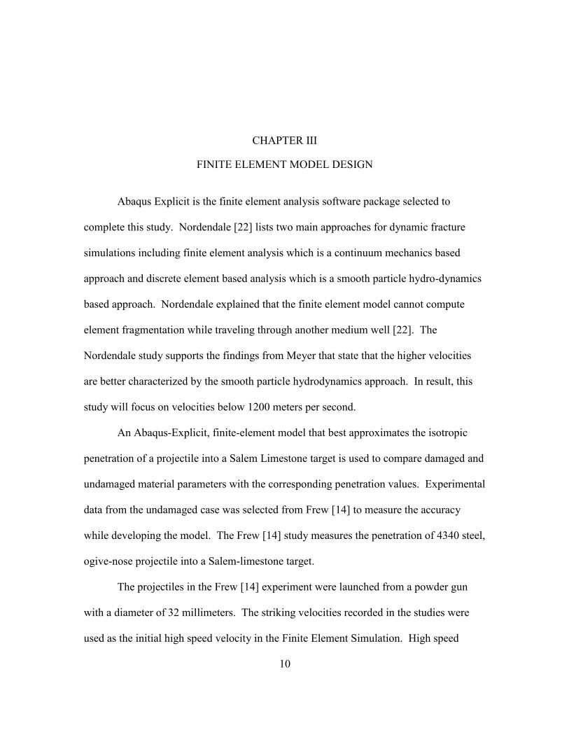
Figure 3.1 Abaqus Projectile Sketch
The projectile is cylindrical nosed with an ogive, edge constricts to a point,
shaped nose. Given the relatively small deformation, a rigid body was considered;
however, using a deformable projectile led to more realistic penetration depths in the
Martin [19] study. Martin [19] stated that the deformable projectile rapidly transfers its
kinetic energy into strain energy in the projectile and slab and viscous dissipation energy
13
in the concrete slab. In contrast, the rigid projectile keeps much of its kinetic energy
while penetrating the target.
Johnson, Chapman, Tsembelis, and Proud suggest tuning the mesh to where the
computational strain and result accuracy is acceptable [16]. For the comparison
simulations the mesh was performed with a coarser mesh. The penetration depth seen
with this mesh and compared with the penetration depth in Frew was acceptable. The
mesh study that occurred for the selection of the mesh for the final simulations of will be
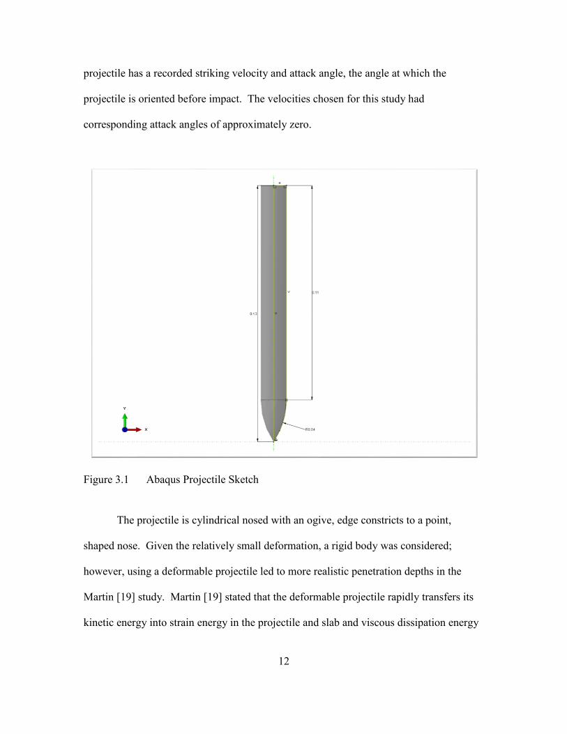
recorded in Chapter 5. The projectile mesh was created by sweeping the mesh around the
radius. No bias was used when creating the mesh. In result, elements of approximately
the same size were created.
The number of elements in the projectile is 1768. The number of nodes is 1998.
An initial velocity of 608 meters per second is assigned to the projectile at the beginning
of the simulation. The Abaqus C3D8R elements were used to discretize the projectile.
14
Figure 3.2 Projectile mesh
Target Part Design
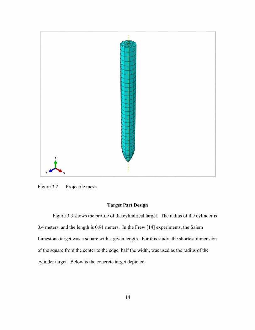
Figure 3.3 shows the profile of the cylindrical target. The radius of the cylinder is
0.4 meters, and the length is 0.91 meters. In the Frew [14] experiments, the Salem
Limestone target was a square with a given length. For this study, the shortest dimension
of the square from the center to the edge, half the width, was used as the radius of the
cylinder target. Below is the concrete target depicted.
15
Figure 3.3 Abaqus Concrete Sketch
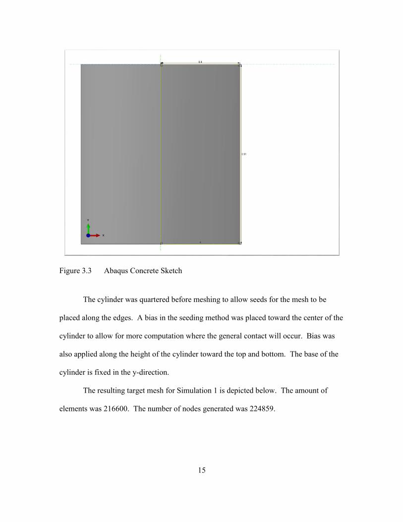
The cylinder was quartered before meshing to allow seeds for the mesh to be
placed along the edges. A bias in the seeding method was placed toward the center of the
cylinder to allow for more computation where the general contact will occur. Bias was
also applied along the height of the cylinder toward the top and bottom. The base of the
cylinder is fixed in the y-direction.
The resulting target mesh for Simulation 1 is depicted below. The amount of
elements was 216600. The number of nodes generated was 224859.
16
Figure 3.4 Target mesh
The Abaqus C3D8R elements were used to discretize the target. The large problem size is attributed more to the concrete slab than the projectile due to the focus on concrete damage.
The axisymmetric elements, CAX4R, was considered for this analysis. These
elements are solid, two-dimensional elements with four nodes. The same analysis that
was created for the three dimensional elements C3D8R and C3D10M was created using
the CAX4R elements for comparison. The entry crater shape for the axisymmetric
element was barely the diameter of the projectile itself. In addition, the resistance
17
through the concrete cylinder was substantially less than the three dimensional elements.
This lead to the hypothesis that the axisymmetric elements were not modeling the
confining stresses as well as the three dimensional elements. Consequentially, the
modeling space selected was three dimensional.
Mesh and Element
Abaqus Explicit uses the central difference or Forward Euler integration method
[1]. The Central Difference method of integration is calculated by the Trapezoidal Rule
which averages the beginning and ending solution for the time increment. The program
uses this method to calculate from the known boundary conditions to the unknown
values. The Central Difference integration method is often used for finite-element, non-
linear, dynamic analysis.
The main advantage of the central difference integration method is the mass
matrix. In the central difference method, the mass matrix is a diagonal matrix which
eliminates the need to perform a triangular factorization [4]. The main disadvantage of
this integration method is the time step being restricted to smaller than critical time step.
Error is introduced to every time step that becomes even slightly larger than the critical
time step for the system. Error can be accumulated during a few time steps; the error in
the solution would not be blatantly apparent.
The time step must also be adjusted to ensure that the delta time is never larger
than half the natural period [4]. Abaqus explicit analysis requires very small time
increments proportional to the time that the stress wave takes to cross the smallest mesh
element [19]. Abaqus determines the step size from the smallest element in the finite
element model. Therefore, a finer mesh and resulting element size for the target would
18
need to be selected to avoid the potential error. For the purpose of comparing material
models, a courser mesh was chosen for quicker simulation time for Chapter 4
simulations. To determine this allowable size for the final mesh simulations, a mesh
refinement study was conducted in Chapter 5.
Elements
Finite element analysis is the numerical approximation of a part by discretization
into elements that can be solved individually from known boundary values until the
whole system is solved. Linear and quadratic elements are used in this study to discretize
the parts. In Abaqus Explicit, the linear 3-D elements are cube shaped with nodes on the
corners. Quadratic elements in Abaqus Explicit are pyramid shaped with nodes at the
corners and mid-spans of the edges.
In finite element analysis, strain is constant for a linear element. Strain is
approximated as a linear function for a quadratic element. Martin [19] only uses the
Abaqus linear elements for analysis and comparison. In this study, linear and quadratic
elements are both used to determine the best numerical analysis method to approximate
the high rate compression occurring during monotonic impact.
Two element types, C3D8R and C3D10M, are selected. The Abaqus C3D8R
elements are continuum, 3-D, 8-node, reduced integration elements. Also, these linear,
hexahedral elements are compatible with Abaqus Explicit. The Abaqus C3D10M
elements are continuum, 3-D, 10-node, modified elements. This element type is also the
only three-dimensional element offered in Abaqus Explicit. Martin [19] uses only
C3D8R to determine stress, strain, and energy components.
19
Projectile Material Model
The classic metal plasticity model was used to model the steel, ogive projectile.
Material parameters were taken from Martin [15]. A simple model of density, elasticity,
and plasticity to reduce the computational time but still maintain the benefit of a
deformable projectile and its transfer of kinetic energy was selected for the steel material
model. The parameters used are tabularized below.
Table 3.2 Steel Material Parameters
Steel Properties Plastic
Density Yield Stress Plastic Strain
7850 Kg/m3 2.2e+08 Pa 0 m/m
Elastic 3.2e+08 Pa 0.25 m/m
Elastic Modulus Poisson’s Ratio 3.7e+08 Pa 0.5 m/m
1.99e+11 Pa 0.3 m/m 3.8e+08 Pa 1 m/m
Concrete Material Models
Three material models are options in Abaqus explicit for modeling
concrete/quasi-brittle materials: brittle cracking for concrete material model, concrete
damaged plasticity material model, and the Holmquist-Johnson-Cook for concrete
material model. All three material models were explored to provide confidence in the
developed finite element model. The energy balances during the simulation and their
ability to accurately predict penetration depth were examined. Previous studies have
compared the concrete damaged plasticity model and the brittle cracking model for their
applications, but none have compared them with the Holmquist Johnson Cook material
model for concrete while in this specific application.
20
Concrete Damaged Plasticity Material Model Setup in Abaqus
The concrete damaged plasticity material model assumes linear elastic behavior
under compression until the initial yield stress is obtained. Then, gradual stress
hardening occurs until the ultimate stress is reached. The strength then begins to
gradually decrease from the ultimate stress due to strain softening. Once the strain
softening strength is reached again, the strength begins to sharply decrease and level to
zero. Tension is linear elastic until the failure stress upon which the strength starts to
decrease first sharp and then gradually to zero. In addition, the model accounts for
tension after compressive damage has been incurred with user modifiable variables.
Strain rate and failure by crushing is also considered for this model. A factor
exists to account for the strain rate. This model has significant strain rate sensitivity that
results in an increase of the concrete’s peak strength. Failure occurs by the collapse and
consolidation of the voids in concrete when large hydrostatic pressures are present that
prevent crack propagation. A modeled part is expected to fail by tensile cracking or
crushing in compression when modeled using this material model. The concrete
damaged plasticity model is intended for use in problems with low confining pressures
and dynamic or cyclic loading conditions [10].
Both the concrete damaged plasticity and the brittle cracking for concrete material
constitutive models use Hillerborg's fracture energy proposal to define the energy
dissipated while forming a crack. Bazant [7] recommends analysis types based on the
dimension of the structure being analyzed. This paper analyzes the high rate penetration
of a Salem limestone target, and Bazant recommends nonlinear quasi-brittle fracture
mechanics for a concrete slab of a thickness equal to fifty centimeters [7]. Hillerborg’s
21
cohesive crack model is one such nonlinear quasi-brittle fracture mechanics analysis
method.
Taylor [24] also used a plasticity-based damage model to simulate high rate
monotonic loading corresponding to this model. Meyer [20] examined the performance
of the concrete damaged plasticity and brittle cracking for concrete model for initial
loading on concrete, but he did not examine the effectiveness of this model in simulating
deep penetration of a concrete target. The concrete damaged plasticity material model
parameters were selected from Martin [19]. The parameters are tabularized below.
Table 3.3 Martin [19] Concrete Damaged Plasticity Material Properties
Concrete Damaged Plasticity (CDP) Elastic
Elastic Modulus Poisson’s Ratio 3.1027E+10 Pa 0.2 m/m
Yield Stress Inelastic Strain 13.0E+6 Pa 0.0 m/m 24.1E+6 Pa 0.001 m/m
Concrete Tension Stiffening Displacement
Yield Stress Displacement 2.9E+6 Pa 0 m
1.94393E+6 Pa 0.000066185 m 1.30305E+6 Pa 0.00012286 m 0.873463E+6 Pa 0.000173427 m
0.5855E+6 Pa 0.00022019 m 0.392472E+6 Pa 0.000264718 m 0.263082E+6 Pa 0.000308088 m 0.176349E+6 Pa 0.00035105 m 0.11821E+6 Pa 0.000394138 m
22
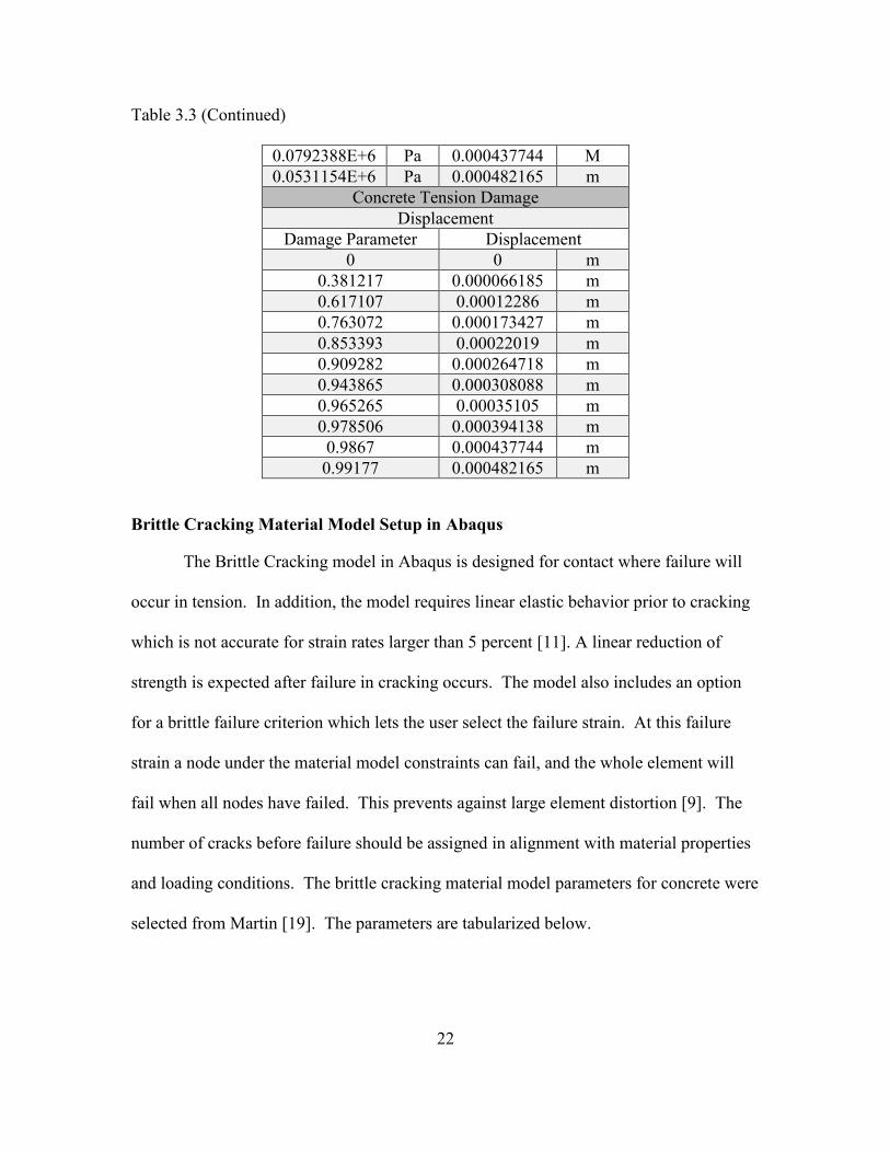
Table 3.3 (Continued)
0.0792388E+6 Pa 0.000437744 M 0.0531154E+6 Pa 0.000482165 m
Concrete Tension Damage Displacement
Damage Parameter Displacement 0 0 m
0.381217 0.000066185 m 0.617107 0.00012286 m 0.763072 0.000173427 m 0.853393 0.00022019 m 0.909282 0.000264718 m 0.943865 0.000308088 m 0.965265 0.00035105 m 0.978506 0.000394138 m 0.9867 0.000437744 m 0.99177 0.000482165 m
Brittle Cracking Material Model Setup in Abaqus
The Brittle Cracking model in Abaqus is designed for contact where failure will
occur in tension. In addition, the model requires linear elastic behavior prior to cracking
which is not accurate for strain rates larger than 5 percent [11]. A linear reduction of
strength is expected after failure in cracking occurs. The model also includes an option
for a brittle failure criterion which lets the user select the failure strain. At this failure
strain a node under the material model constraints can fail, and the whole element will
fail when all nodes have failed. This prevents against large element distortion [9]. The
number of cracks before failure should be assigned in alignment with material properties
and loading conditions. The brittle cracking material model parameters for concrete were
selected from Martin [19]. The parameters are tabularized below.
23
Table 3.4 Brittle Cracking for Concrete Material Parameters Martin [19]
Density 0.263082 Pa 0.0006 m/m 2.5650E-09 Kg/m3 0.176349 Pa 0.0007 m/m
ELASTIC, ISOTROPIC 0.11821 Pa 0.0008 m/m Elastic Modulus Poisson’s Ratio 0.0792388 Pa 0.0009 m/m 20800.0 Pa 0.175 m/m 0.0531154 Pa 0.001 m/m
BRITTLE CRACKING, Strain BRITTLE SHEAR Direct Stress
After Cracking Direct Cracking
Strain Shear Retention
Factor Crack Opening
Strain 2.9 Pa 0 m/m 1.0 0.0 m/m
1.94393 Pa 0.0001 m/m 0.5 0.001 m/m 1.30305 Pa 0.0002 m/m 0.25 0.002 m/m 0.873463 Pa 0.0003 m/m 0.125 0.003 m/m 0.5855 Pa 0.0004 m/m BRITTLE FAILURE, CRACKS=1
0.392472 Pa 0.0005 m/m 1.0E-6
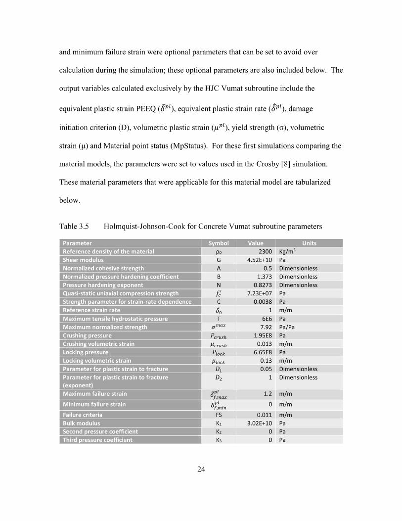
Holmquist-Johnson-Cook for Concrete Material Model
In Abaqus Explicit, the Holmquist-Johnson-Cook (HJC) Constitutive Material
Model for Concrete requires the following parameters in a, Dassault Systems [12], Vumat
subroutine: the reference density of the material (ρ0), shear modulus (G), normalized
ETOTAL, and ALLVD are measured during the Abaqus Explicit simulation. However,
after removing the energies that do not contribute, the following is equal to ETOTAL: the
sum of ALLIE, ALLVD, and ALLKE where ALLIE is equal to the sum of ALLAE,
ALLPD, and ALLSE. All further discussions of energy will be on this reduced energy
equation.
Holmquist-Johnson-Cook
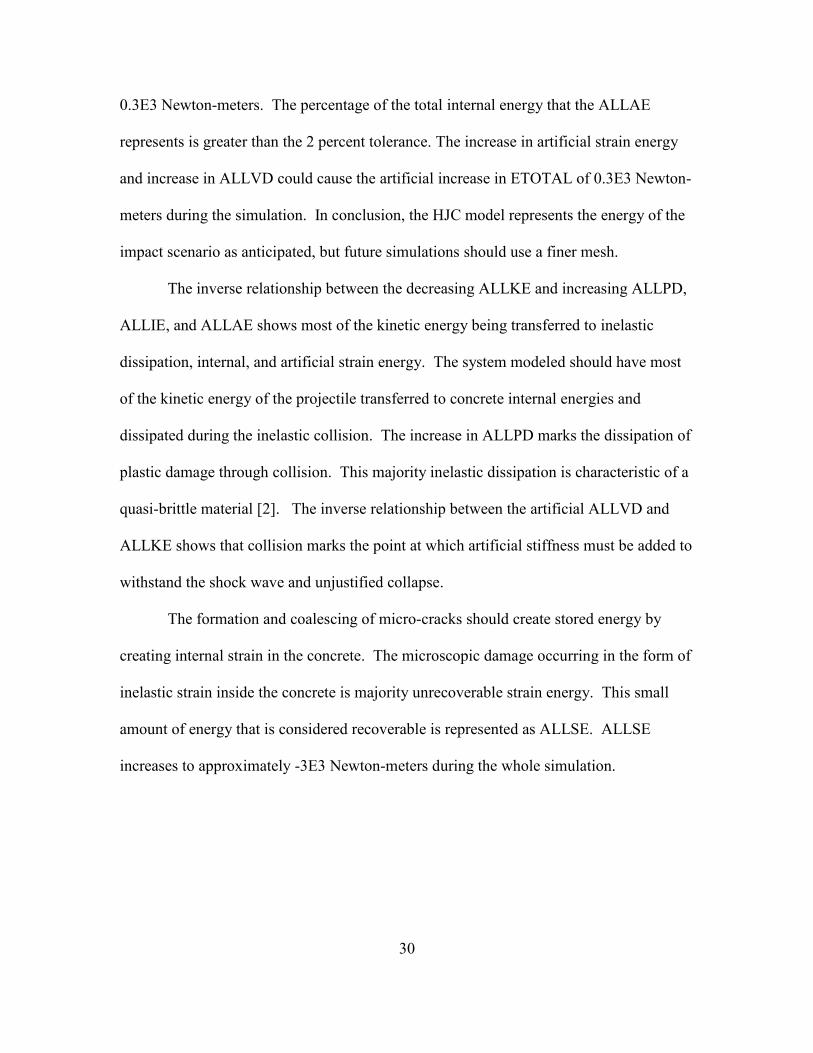
Figure 4.1 represents the changing energy distributions during monotonic impact.
The ALLKE is decreasing linearly from 20E3 to 4E3 Newton-meters as ALLPD and
ALLIE are increasing linearly from 0 to 12.5E3 Newton-meters and from 0 to 15E3
Newton-meters during a 0.25 milliseconds timespan. ALLPD continues to increase and
never reaches a maximum during the simulation timespan. The ALLIE increases to a
maximum of 18E3 Newton-meters at approximately 0.4 milliseconds. At completion, the
value for ALLPD is 19E3 Newton-meters. After 0.25 milliseconds, the ALLKE
continues to decrease until a minimum at 0.4 milliseconds and 2E3 Newton-meters.
The ALLAE increases to a maximum of 3E3 Newton-meters at approximately
0.23 milliseconds. The ALLVD increases during the full, time span to approximately
30
0.3E3 Newton-meters. The percentage of the total internal energy that the ALLAE
represents is greater than the 2 percent tolerance. The increase in artificial strain energy
and increase in ALLVD could cause the artificial increase in ETOTAL of 0.3E3 Newton-
meters during the simulation. In conclusion, the HJC model represents the energy of the
impact scenario as anticipated, but future simulations should use a finer mesh.
The inverse relationship between the decreasing ALLKE and increasing ALLPD,
ALLIE, and ALLAE shows most of the kinetic energy being transferred to inelastic
dissipation, internal, and artificial strain energy. The system modeled should have most
of the kinetic energy of the projectile transferred to concrete internal energies and
dissipated during the inelastic collision. The increase in ALLPD marks the dissipation of
plastic damage through collision. This majority inelastic dissipation is characteristic of a
quasi-brittle material [2]. The inverse relationship between the artificial ALLVD and
ALLKE shows that collision marks the point at which artificial stiffness must be added to
withstand the shock wave and unjustified collapse.
The formation and coalescing of micro-cracks should create stored energy by
creating internal strain in the concrete. The microscopic damage occurring in the form of
inelastic strain inside the concrete is majority unrecoverable strain energy. This small
amount of energy that is considered recoverable is represented as ALLSE. ALLSE
increases to approximately -3E3 Newton-meters during the whole simulation.
31
Figure 4.1 Holmquist-Johnson-Cook for concrete energy
Concrete Damaged Plasticity
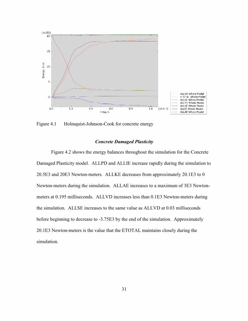
Figure 4.2 shows the energy balances throughout the simulation for the Concrete
Damaged Plasticity model. ALLPD and ALLIE increase rapidly during the simulation to
20.5E3 and 20E3 Newton-meters. ALLKE decreases from approximately 20.1E3 to 0
Newton-meters during the simulation. ALLAE increases to a maximum of 3E3 Newton-
meters at 0.195 milliseconds. ALLVD increases less than 0.1E3 Newton-meters during
the simulation. ALLSE increases to the same value as ALLVD at 0.03 milliseconds
before beginning to decrease to -3.75E3 by the end of the simulation. Approximately
20.1E3 Newton-meters is the value that the ETOTAL maintains closely during the
simulation.
32
Figure 4.2 Concrete Damaged Plasticity energy
The energy relationships behaved congruently to the Holmquist-Johnson-Cook
material model except when ALLKE decreases rapidly to zero. The whole simulation
ends more rapidly than for the Holmquist-Johnson-Cook model because the initial kinetic
energy is maintained more after 0.15 milliseconds with the HJC model. This is because
the concrete damaged plasticity model does not allow finite elements under significant
stresses and strains to fail which gives the structure increased artificial stiffness. In
result, an unrealistically low penetration depth is seen for this concrete material model.
Overall, the energy is well represented in initial impact, so the model would represent
concrete well for simulations other than penetration.
Brittle Cracking for Concrete
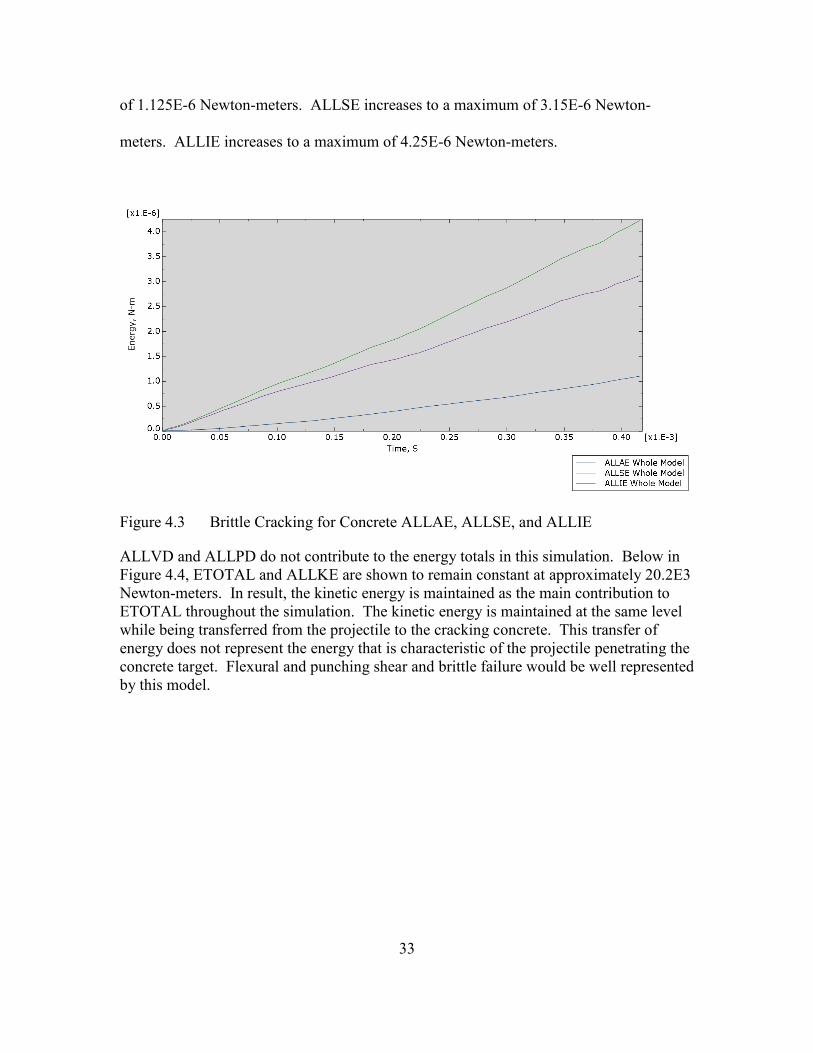
Figure 4.3 shows the ALLAE, ALLSE, and ALLIE energy distribution for the
penetration simulations using the Brittle Cracking for Concrete model. ALLAE, ALLSE,
and ALLIE increases minimally during the simulation. ALLAE increases to a maximum
33
of 1.125E-6 Newton-meters. ALLSE increases to a maximum of 3.15E-6 Newton-
meters. ALLIE increases to a maximum of 4.25E-6 Newton-meters.
Figure 4.3 Brittle Cracking for Concrete ALLAE, ALLSE, and ALLIE
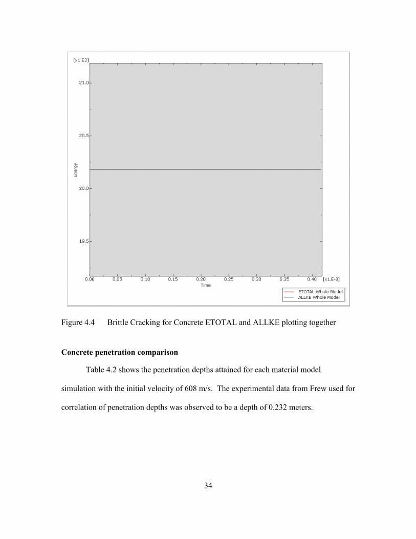
ALLVD and ALLPD do not contribute to the energy totals in this simulation. Below in Figure 4.4, ETOTAL and ALLKE are shown to remain constant at approximately 20.2E3 Newton-meters. In result, the kinetic energy is maintained as the main contribution to ETOTAL throughout the simulation. The kinetic energy is maintained at the same level while being transferred from the projectile to the cracking concrete. This transfer of energy does not represent the energy that is characteristic of the projectile penetrating the concrete target. Flexural and punching shear and brittle failure would be well represented by this model.
34
Figure 4.4 Brittle Cracking for Concrete ETOTAL and ALLKE plotting together
Concrete penetration comparison
Table 4.2 shows the penetration depths attained for each material model
simulation with the initial velocity of 608 m/s. The experimental data from Frew used for
correlation of penetration depths was observed to be a depth of 0.232 meters.
35
Table 4.2 Displacement from time 0 to 3.7334E-04 seconds, V = 608 m/s
HJC for Concrete Concrete Damage Plasticity
Brittle Cracking
m m m
0.160738 0.00280822 0.227525
The Holmquist Johnson Cook for concrete and Concrete Damage Plasticity models completed penetration during the simulation time. In contrast, the Brittle Cracking for Concrete material model does not complete penetration during the penetration time. Instead the projectile and punched-shear-failed concrete continues motion past the simulation time.
Figure 4.5 shows the penetration depth of the projectile at the end time using the
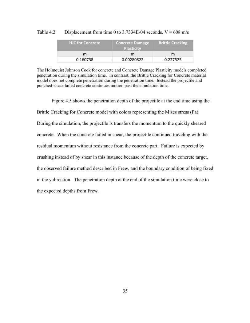
Brittle Cracking for Concrete model with colors representing the Mises stress (Pa).
During the simulation, the projectile is transfers the momentum to the quickly sheared
concrete. When the concrete failed in shear, the projectile continued traveling with the
residual momentum without resistance from the concrete part. Failure is expected by
crushing instead of by shear in this instance because of the depth of the concrete target,
the observed failure method described in Frew, and the boundary condition of being fixed
in the y direction. The penetration depth at the end of the simulation time were close to
the expected depths from Frew.
36
Figure 4.5 Brittle Cracking for Concrete penetration depth and Mises stress
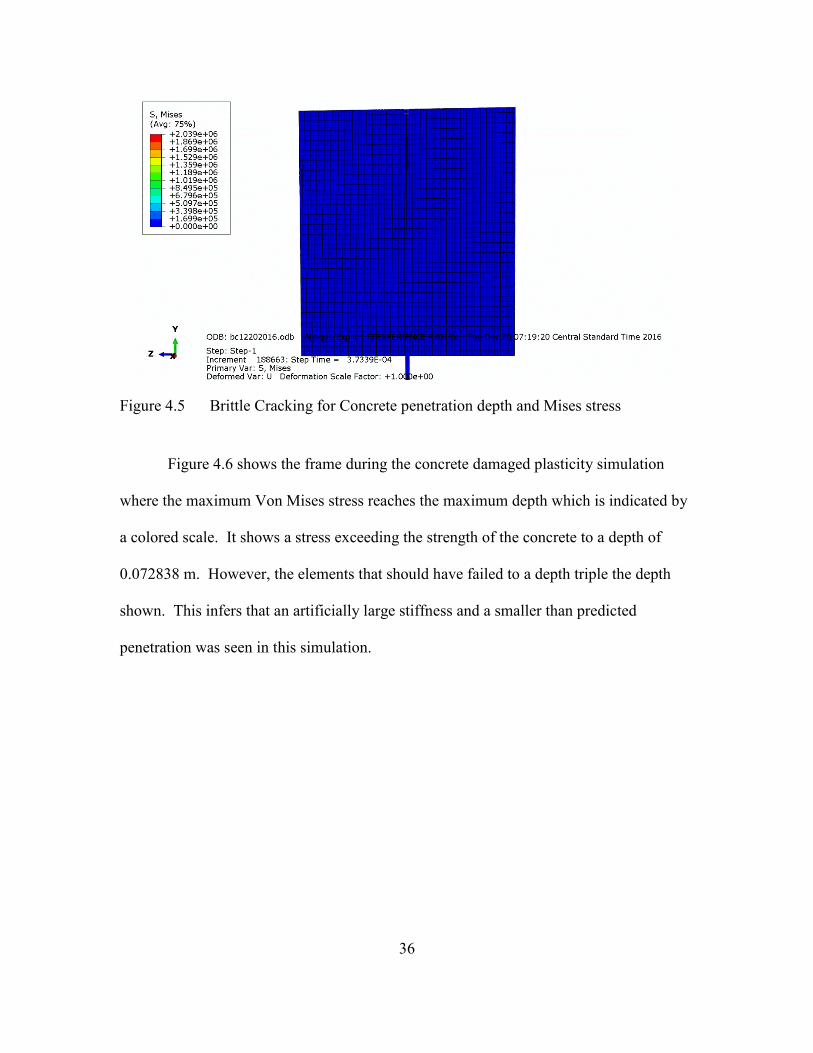
Figure 4.6 shows the frame during the concrete damaged plasticity simulation
where the maximum Von Mises stress reaches the maximum depth which is indicated by
a colored scale. It shows a stress exceeding the strength of the concrete to a depth of
0.072838 m. However, the elements that should have failed to a depth triple the depth
shown. This infers that an artificially large stiffness and a smaller than predicted
penetration was seen in this simulation.
37
Figure 4.6 Concrete Damaged Plasticity penetration depth and Mises stress
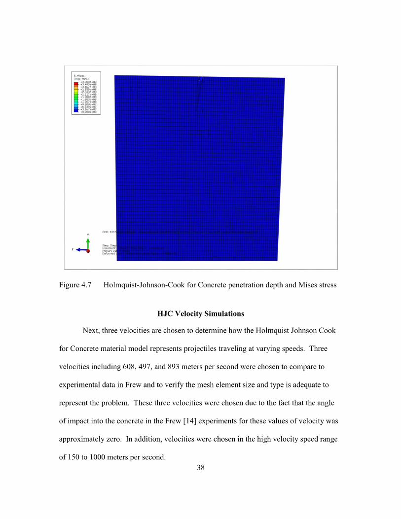
Figure 4.7 shows the last frame of the Holmquist Johnson Cook simulation with
colors representing Von Mises stresses (Pa). Of the three models, the HJC simulations’
penetration depth of the projectile best represents the experimental penetration depth.
This is due to the energy distribution corresponding to the boundary conditions and
quasi-brittle material behavior during the simulation. In addition, the penetration depth
was the closest match to the known experimental penetration depth from Frew. Thus, the
Holmquist Johnson Cook for Concrete material model is chosen to simulate future impact
events in this study.
38
Figure 4.7 Holmquist-Johnson-Cook for Concrete penetration depth and Mises stress
HJC Velocity Simulations
Next, three velocities are chosen to determine how the Holmquist Johnson Cook
for Concrete material model represents projectiles traveling at varying speeds. Three
velocities including 608, 497, and 893 meters per second were chosen to compare to
experimental data in Frew and to verify the mesh element size and type is adequate to
represent the problem. These three velocities were chosen due to the fact that the angle
of impact into the concrete in the Frew [14] experiments for these values of velocity was
approximately zero. In addition, velocities were chosen in the high velocity speed range
of 150 to 1000 meters per second.
39
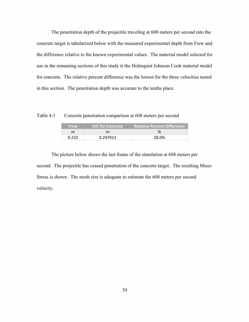
The penetration depth of the projectile traveling at 608 meters per second into the
concrete target is tabularized below with the measured experimental depth from Frew and
the difference relative to the known experimental values. The material model selected for
use in the remaining sections of this study is the Holmquist Johnson Cook material model
for concrete. The relative percent difference was the lowest for the three velocities tested
in this section. The penetration depth was accurate to the tenths place.
Table 4.3 Concrete penetration comparison at 608 meters per second
Frew HJC for Concrete Relative Percent Difference
m m %
0.232 0.297013 28.0%
The picture below shows the last frame of the simulation at 608 meters per
second. The projectile has ceased penetration of the concrete target. The resulting Mises
Stress is shown. The mesh size is adequate to estimate the 608 meters per second
velocity.
40
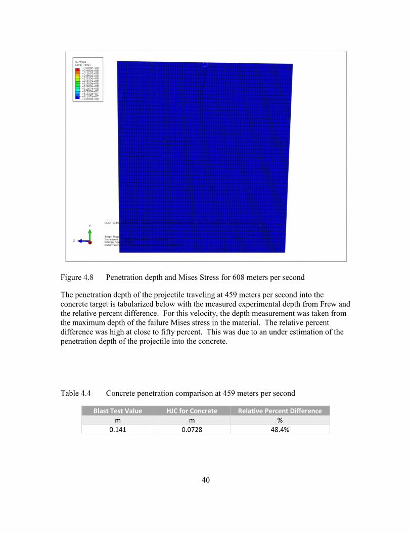
Figure 4.8 Penetration depth and Mises Stress for 608 meters per second
The penetration depth of the projectile traveling at 459 meters per second into the concrete target is tabularized below with the measured experimental depth from Frew and the relative percent difference. For this velocity, the depth measurement was taken from the maximum depth of the failure Mises stress in the material. The relative percent difference was high at close to fifty percent. This was due to an under estimation of the penetration depth of the projectile into the concrete.
Table 4.4 Concrete penetration comparison at 459 meters per second
Blast Test Value HJC for Concrete Relative Percent Difference
m m %
0.141 0.0728 48.4%
41
The picture below shows the frame of the simulation with the maximum depth of
Mises Stress above the material failure stress resulting from the projectile traveling at 459
meters per second. Visually the elements did not fail as expected at this velocity;
however, the failure Mises stress reflects depths accurate to the tenths which reflects
positively upon the mesh size for this velocity even though the relative percent difference
is high. The simulation completed with the full penetration of the projectile into the
concrete. The last frame of the simulation depicts that cessation.
Figure 4.9 Penetration depth and Mises Stress for 459 meters per second
42
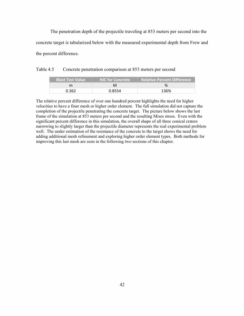
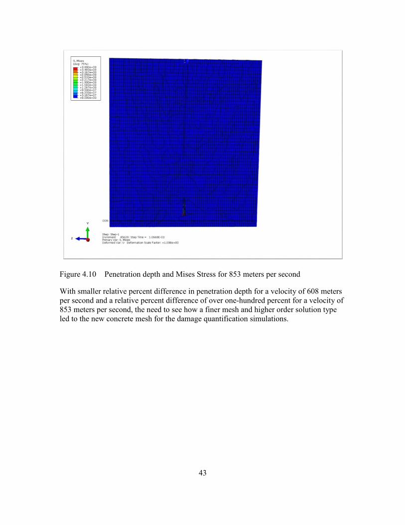
The penetration depth of the projectile traveling at 853 meters per second into the
concrete target is tabularized below with the measured experimental depth from Frew and
the percent difference.
Table 4.5 Concrete penetration comparison at 853 meters per second
Blast Test Value HJC for Concrete Relative Percent Difference
m M %
0.362 0.8554 136%
The relative percent difference of over one hundred percent highlights the need for higher velocities to have a finer mesh or higher order element. The full simulation did not capture the completion of the projectile penetrating the concrete target. The picture below shows the last frame of the simulation at 853 meters per second and the resulting Mises stress. Even with the significant percent difference in this simulation, the overall shape of all three conical craters narrowing to slightly larger than the projectile diameter represents the real experimental problem well. The under estimation of the resistance of the concrete to the target shows the need for adding additional mesh refinement and exploring higher order element types. Both methods for improving this last mesh are seen in the following two sections of this chapter.
43
Figure 4.10 Penetration depth and Mises Stress for 853 meters per second
With smaller relative percent difference in penetration depth for a velocity of 608 meters per second and a relative percent difference of over one-hundred percent for a velocity of 853 meters per second, the need to see how a finer mesh and higher order solution type led to the new concrete mesh for the damage quantification simulations.
44
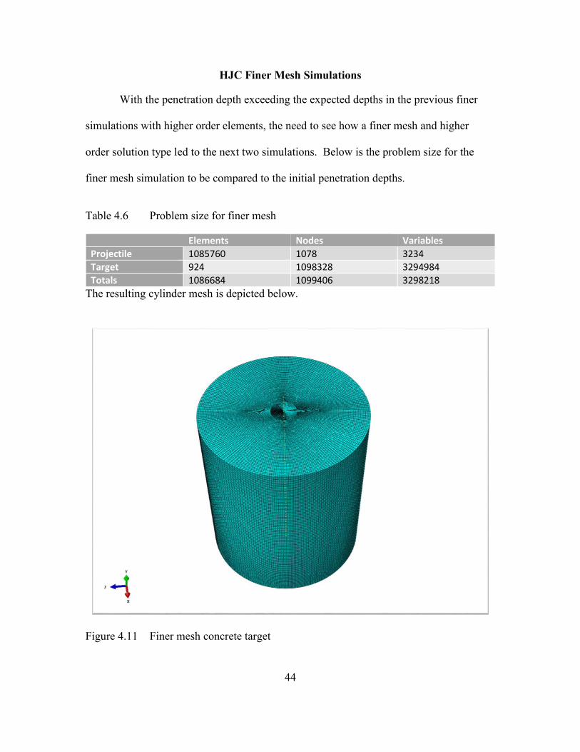
HJC Finer Mesh Simulations
With the penetration depth exceeding the expected depths in the previous finer
simulations with higher order elements, the need to see how a finer mesh and higher
order solution type led to the next two simulations. Below is the problem size for the
finer mesh simulation to be compared to the initial penetration depths.
Table 4.6 Problem size for finer mesh
Elements Nodes Variables
Projectile 1085760 1078 3234
Target 924 1098328 3294984
Totals 1086684 1099406 3298218
The resulting cylinder mesh is depicted below.
Figure 4.11 Finer mesh concrete target
45
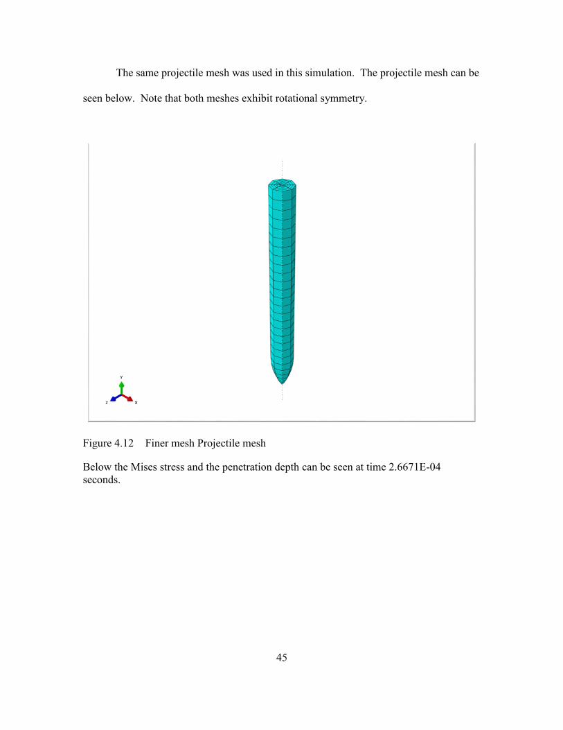
The same projectile mesh was used in this simulation. The projectile mesh can be
seen below. Note that both meshes exhibit rotational symmetry.
Figure 4.12 Finer mesh Projectile mesh
Below the Mises stress and the penetration depth can be seen at time 2.6671E-04 seconds.
46
Figure 4.13 Finer mesh penetration V=608 m/s
The depth at a time of 2.6671E-04 seconds for the original mesh for the material model comparisons for HJC was 0.09 meters. The new depth resulting from the finer mesh is 0.12 meters. The resulting increase of depth from the original mesh is approximately 33 percent. This indicates that the finer mesh will contribute to a small overestimation of the depth. The next variable to be checked is the effect of higher order elements.
HJC Quadratic, tetrahedral elements simulations
The same projectile mesh is used for this simulation with a cylinder composed of
quadratic, tetrahedral elements. The problem size is described below in the table in terms
of number of elements, nodes, and variables.
47
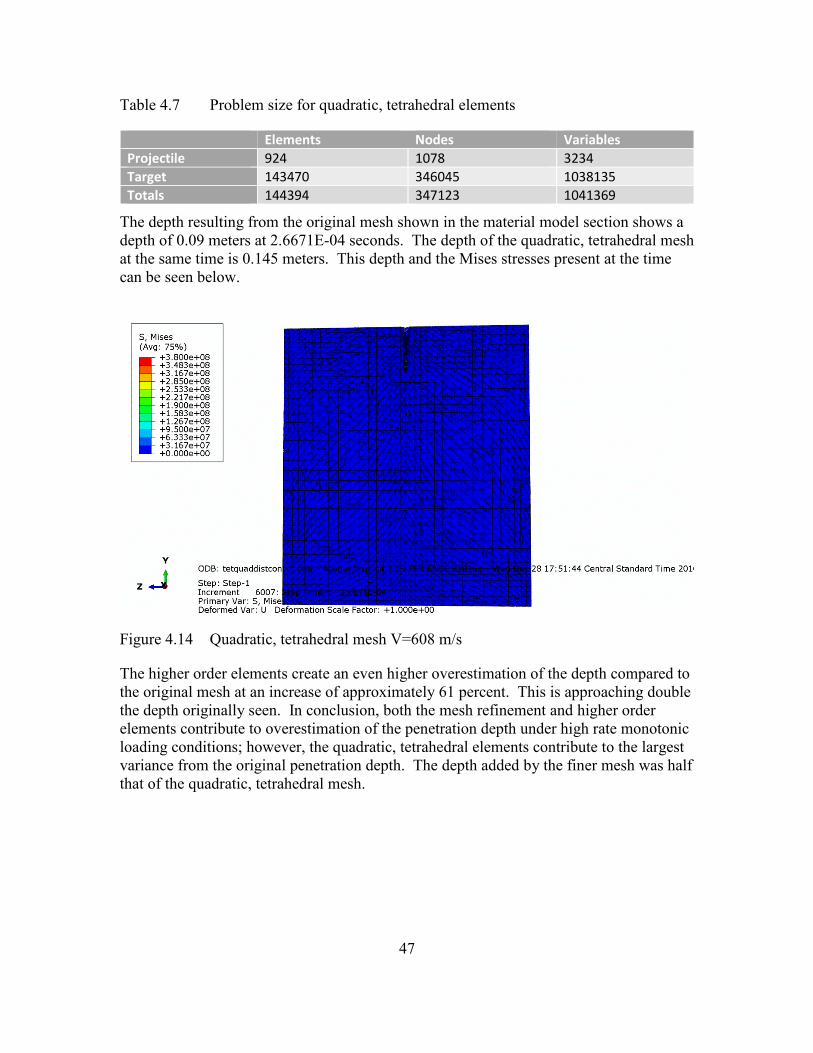
Table 4.7 Problem size for quadratic, tetrahedral elements
Elements Nodes Variables
Projectile 924 1078 3234
Target 143470 346045 1038135
Totals 144394 347123 1041369
The depth resulting from the original mesh shown in the material model section shows a depth of 0.09 meters at 2.6671E-04 seconds. The depth of the quadratic, tetrahedral mesh at the same time is 0.145 meters. This depth and the Mises stresses present at the time can be seen below.
Figure 4.14 Quadratic, tetrahedral mesh V=608 m/s
The higher order elements create an even higher overestimation of the depth compared to the original mesh at an increase of approximately 61 percent. This is approaching double the depth originally seen. In conclusion, both the mesh refinement and higher order elements contribute to overestimation of the penetration depth under high rate monotonic loading conditions; however, the quadratic, tetrahedral elements contribute to the largest variance from the original penetration depth. The depth added by the finer mesh was half that of the quadratic, tetrahedral mesh.
48
Mesh Refinement Study
The graph shown below shows how the mesh’s ability to predict the penetration
depth converges on blank value.
The energy can be seen to be.
49
CHAPTER V
HJC DAMAGED MATERIAL SIMULATIONS
The first simulations to perform with the developed finite element model is
uniaxial compression simulations. These quasi-static simulations were used to correlate
the unconfined compressive strengths seen in Crosby to the model and to determine the
correlation between the damage parameter and a continuous range of micro-crack
damage. Then, penetration simulations are run with three damage coefficients
corresponding to the finite levels of damage stated in Crosby [8].
Uniaxial Compression Simulation
Elements with varying material parameters and damage level can be compared for
strength to determine if the results show high mesh dependence. The mean peak
principle stress difference for no, low, and high damage is 72.3, 65.3, and 45.7 Mega
Pascal in Crosby [8]. The less complex uniaxial compression tests are intended to
eliminate the question of material parameter settings contributing to the deeper
penetration depths seen in the latest simulations. Changes in conclusions with regard to
the element type and size effect and damage levels effect on penetration resistance of
concrete will be presented in this section. In addition, methods to accelerate the
simulation time will be evaluated, and a method will be chosen and examined for
sensitivity.
50
The diameter of the concrete sample is 50.8 millimeters, and the height of the
sample is 114 millimeters. The cylinder has the same mesh seen in previous sections.
The pressure load is applied to the surface of the cylinder at a rate of 6000 Newtons per
Second. The loading rate is applied as a smooth step.
The limitation is that there are only finite levels of damage to be represented by
changing the material parameters found in Crosby [8]. Abaqus has the option of setting
an initial damage level by specifying an initial damage constant for elements in the
cylinder instance. To eliminate this limitation, a link between this damage constant and
the material characteristics seen in uniaxial compression tests needs to be established.
This is done by varying the damage constant by 0.1 from 0 to 0.9 in the same model
created above for undamaged Salem Limestone material parameters.
Figure 5.1 shows the stress versus strain relationship for damage levels from 0 to
0.9 incrementing by 0.1. The trend of linearly increasing unconfined compressive
strength can be seen. In addition, the slope of the stress versus strain remains constant.
Further simulations could be completed to incorporate varying moduli in the simulations
because the results would fit the experimental stress strain curve closer. This linear
relationship of the maximum unconfined compressive strength and damage coefficient
will be examined further in the next figure.
51
Figure 5.1 Stress versus Strain for Varying Damage Constants
In Figure 5.2, the relationship between the unconfined compressive strength and
the initial damage is shown. The scatter of points is linked by lines. The scatter is linear
in nature, so a linear fit will be applied to the data in the next graph. This is valuable
because the damage coefficient from the Holmquist-Johnson-Cook Constitutive model
can now be linked to an unconfined compressive strength.
52
Figure 5.2 Damage Constant versus Unconfined Compressive Strength
In Figure 5.3, the damage coefficient corresponding to the micro-crack damage
level from Crosby [8] can be determined. The value corresponding to no damage by
micro-cracking is 0.0331. 0.1326 represents the low damage level by micro-cracking,
and the high damage level can be represented by the damage coefficient 0.4223. With
this correlation method, a complete range micro-cracking can be represented for Salem
Limestone by picking the unconfined compressive strength, tracking it horizontally to the
linear fit line, and down to the damage coefficient.
53
Figure 5.3 Initial Damage Values’ Linear Relationship to Micro-crack Damage
Comparison of Damaged Level and Penetration Profile
This section shows the penetration depth profile for the total time span for 608
meters per second. The node at the projectile point was tracked during the simulation for
the penetration depth. In addition, twenty frames are calculated by Abaqus for each
penetration simulation.
54
CHAPTER VI
CONCLUSIONS
An Abaqus Explicit finite element model was developed to model a projectile and
target from Frew [14]. The model was developed by accessing the material model
options for the target and projectile, the element options, and mesh options. A classic
metal plasticity material model was selected for the projectile due to other material
models causing increased computation time. The HJC material model was selected as the
optimal material model for representing quasi-brittle material due to its accurate
representation of the penetration depth, crater shape, and energy balances throughout the
simulation. Due to the energy balances seen, additional mesh refinement was
recommended with linear elements for the subsequent simulations for high-speed
resistance to monotonic impact. This refinement was completed with a mesh refinement
study which compared the refinement versus penetration depth and the new energy
balances.
Quasi-static, uniaxial compression tests were performed to correlate the HJC
damage coefficient to tested levels of micro-cracking. The coefficients that were
determined to be representative of the damage level were then used in penetration
simulations. The penetration simulations helped to determine the different resistances of
concrete samples with high, low, and no micro-crack damage. The penetration depth
versus simulation time seen reflected these results
55
With tension or cyclic loading as an additional factor, micro cracks would exhibit
more of a hindrance in accurately modeling strength. Further research could be done to
develop a finite element material model to implement the Modified Holmquist Johnson
Cook Material Model developed in Crosby. Material characteristics for damaged
material would be more accurately predicted for an evolving, continuous range of
damage states instead of singularity no, low, and high damage.
56
REFERENCES
[1] ABAQUS, inc. (2005). Overview of Abaqus Explicit. Retrieved January 19, 2017, from http://imechanica.org/files/0-overview%20Explicit.pdf
[2] BAERA, C., SZILAGYI, H., MIRCEA, C., CRIEL, P., & De BELIE, N. (2016). CONCRETE STRUCTURES UNDER IMPACT LOADING: GENERAL ASPECTS. Urbanism. Architecture. Constructions / Urbanism. Arhitectura. Constructii, 7(3), 239-250.
[3] Banthia, N. P. (1987), Impact resistance of concrete, Doctoral Thesis, University of British Columbia, Vancouver, Canada.
[4] Bathe, K. J. (1982). Finite element procedures in engineering analysis.
[5] Baxter, J. W. (1960). Salem limestone in southwestern Illinois. Circular no. 284.
[6] Bazant, Z. P., & Planas, J. (1997). Fracture and size effect in concrete and other quasibrittle materials (Vol. 16). CRC press.
[7] Bažant, Z. P. (2002). Concrete fracture models: testing and practice. Engineering fracture mechanics, 69(2), 165-205.
[8] Crosby, Z. K. (2013). Effects of thermally-induced microcracking on the quasi-static and dynamic response of Salem limestone (Doctoral dissertation, MISSISSIPPI STATE UNIVERSITY).
[9] Dassault Systèmes Simulia Corp. (2010). 20.6.2 Cracking model for concrete. In Abaqus Analysis User's Manual (6.10 ed.). Retrieved from https://www.sharcnet.ca/Software/Abaqus610/Documentation/docs/v6.10/books/usb/default.htm?startat=pt05ch20s06abm37.html
[10] Dassault Systèmes Simulia Corp. (2014). 23.6.3 Concrete damaged plasticity. In Abaqus analysis user's guide (6.14 ed.). Retrieved from http://129.97.46.200:2080/v6.14/books/usb/default.htm?startat=pt05ch23s06abm39.html
[11] Dassault Systèmes Simulia Corp. (2010). 19.2.1 Linear elastic behavior. In Abaqus Analysis User's Manual (6.10 ed.). Retrieved from https://www.sharcnet.ca/Software/Abaqus610/Documentation/docs/v6.10/books/usb/default.htm?startat=pt05ch20s06abm37.html
57
[12] Dassault Systèmes Simulia. (2010). VUMAT for the HJC Concrete Model. Retrieved from www.3ds.com.
[13] Forrestal, M. J., Frew, D. J., Hanchak, S. J., & Brar, N. S. (1996). Penetration of grout and concrete targets with ogive-nose steel projectiles. International Journal of Impact Engineering, 18(5), 465-476.
[14] Frew, D. J. (2000). Dynamic response of brittle materials from penetration and split Hopkinson pressure bar experiments.
[15] Holmquist, T. J., Johnson, G. K., & Cook, W. (1993). A computational constitutive model for concrete subjected to large strains, high strain rate, and high pressures. In 14th international symposium on ballistics (Vol. 9, pp. 591-600).
[16] Johnson, D., Chapman, D. J., Tsembelis, K., & Proud, W. G. (2007). THE RESPONSE OF DRY LIMESTONE TO SHOCK-LOADING. AIP Conference Proceedings, 955(1), 1387-1390. doi:10.1063/1.2832984
[17]Khazraiyan, N., Liaghat, G. H., & Khodarahmi, H. (2013). Normal impact of hard projectiles on concrete targets. Structural Concrete, 14(2), 176-183.
[18] Logan, D. L. (2011). A first course in the finite element method. Cengage Learning.
[19] Martin, O. (2010). Comparison of different constitutive models for concrete in ABAQUS/explicit for missile impact analyses. JRC Scientific and Technical Reports.
[20] Meyer, C. S. (2013). Modeling experiments of hypervelocity penetration of adobe by spheres and rods. Procedia Engineering, 58, 138-146.
[21] Nazzal, M., Abu-Farsakh, M., & Mohammad, L. (2007). Laboratory Characterization of Reinforced Crushed Limestone under Monotonic and Cyclic Loading. Journal Of Materials In Civil Engineering, 19(9), 772-783. doi:10.1061/(ASCE)0899-1561(2007)19:9(772)
[22] Nordendale, N. A. (2013). Modeling and Simulation of Brittle Armors Under Impact and Blast Effects (Doctoral dissertation, Vanderbilt University).
[23] Surendranath, H., Oancea, V., & Subbarayalu, S. (2011). Full vehicle durability prediction using Co-Simulation between Implicit and Explicit finite element solvers. Tech. rep., Dassault Systémes Simulia Corp.
[24] Taylor, L. M., Chen, E. P., & Kuszmaul, J. S. (1986). Microcrack-induced damage accumulation in brittle rock under dynamic loading. Computer methods in applied mechanics and engineering, 55(3), 301-320.
58
[25] Zou, F., Fang, Z., & Xia, M. (2016). Study on Dynamic Mechanical Properties of Limestone under Uniaxial Impact Compressive Loads. Mathematical Problems In Engineering, 1-11. doi:10.1155/2016/5207457