103
Copyright by Soovadeep Bakshi 2017

Copyright
by
Soovadeep Bakshi
2017
The Thesis Committee for Soovadeep Bakshicertifies that this is the approved version of the following thesis:
Modeling and Control of Transition Dynamics in a
Two-Piston Toroidal Blood Pump
APPROVED BY
SUPERVISING COMMITTEE:
Raul G. Longoria, Supervisor
Joseph J. Beaman

Modeling and Control of Transition Dynamics in a
Two-Piston Toroidal Blood Pump
by
Soovadeep Bakshi, B.Tech.
Thesis
Presented to the Faculty of the Graduate School of
The University of Texas at Austin
in Partial Fulfillment
of the Requirements
for the Degree of
Master of Science in Engineering
The University of Texas at Austin
May 2017

Acknowledgments
I must first acknowledge my advisor, Prof. Raul Longoria, who has
guided me through my Master’s degree. I have truly learnt a lot from his years
of experience in bond graph-based modeling, which, I believe, has helped me
immensely in the understanding of physical systems. His support and feedback
have meant a lot to me.
Right from my childhood, my family has been extremely supportive of
every major decision that I have taken. As I move on to doctoral studies, I
consider them to be the pillars that prop me up.
Other than my family, I would like to thank the excellent teachers that I
have had at UT Austin, especially Professors Benito Fernandez, Dongmei Chen
and Joseph Beaman, all of whom have helped me understand the fundamentals
of dynamics and control.
New and old friends have helped me out a lot in life, especially those
with whom I have had numerous discussions, both technical and philosophical,
over the past years. Therefore, finally, I would like to thank them because
without them, my research efforts would have been unsuccessful.
iv

Modeling and Control of Transition Dynamics in a
Two-Piston Toroidal Blood Pump
Soovadeep Bakshi, MSE
The University of Texas at Austin, 2017
Supervisor: Raul G. Longoria
Ventricular Assist Devices (VADs) are becoming more and more popu-
lar as a treatment option for patients with weak or failing hearts, and this has
made research into the analysis and control of VADs more necessary. This the-
sis is a study of the modeling and control of transition dynamics of the pistons
in the TORVADTM, a toroidal VAD developed by Windmill Cardiovascular
Systems, Inc. (WCS, Inc., Austin, TX).
The main objective of this thesis is to design a model-based control
strategy for trajectory tracking in the transition phase of the TORVADTM with
minimal oscillations in the control voltages provided to the motors. A bond
graph-based hybrid model of the pump is designed for better understanding
of the fluid-mechanical coupling in the TORVADTM, as well as performance
comparison of the designed controllers. Using a simplified version of the pump
model as the nominal plant, a model-based cascaded controller is designed
and compared with an error-based PID control strategy. Results for specified
v

testing trajectories, and a preliminary robustness analysis of the two control
strategies are presented, and the cascaded control strategy is shown to generate
control voltages which are much less oscillatory than that of the PID control
strategy.
vi

Table of Contents
Acknowledgments iv
Abstract v
List of Tables ix
List of Figures x
Chapter 1. Introduction 1
Chapter 2. Multi-Energetic Pump Model 6
2.1 Components of the Multi-Energetic Model . . . . . . . . . . . 6
2.1.1 Modified Beaman-Breedveld Structure . . . . . . . . . . 7
2.1.2 Loss Models . . . . . . . . . . . . . . . . . . . . . . . . 12
2.1.3 Momentum Transfer Model . . . . . . . . . . . . . . . . 13
2.1.4 Actuator Model . . . . . . . . . . . . . . . . . . . . . . 15
2.2 Complete Fluid Model and State Equations . . . . . . . . . . . 17
2.2.1 Bond Graph Structure of the Pump . . . . . . . . . . . 17
2.2.2 Model States and Equations . . . . . . . . . . . . . . . . 19
2.3 Hybrid Model Modes . . . . . . . . . . . . . . . . . . . . . . . 23
2.3.1 Modes with Obstructed Ports . . . . . . . . . . . . . . . 25
2.3.2 Modes with Shunts . . . . . . . . . . . . . . . . . . . . . 27
2.4 Summary . . . . . . . . . . . . . . . . . . . . . . . . . . . . . . 31
Chapter 3. Control Strategies for Transition Dynamics 32
3.1 Simplified Model for Controller Design . . . . . . . . . . . . . 32
3.1.1 Nominal Models for Normal Operating Conditions . . . 32
3.1.2 Nominal Model for Shunt Cases . . . . . . . . . . . . . . 37
3.2 Controllability and Observability . . . . . . . . . . . . . . . . . 40
vii
3.2.1 Controllability . . . . . . . . . . . . . . . . . . . . . . . 40
3.2.2 Observability . . . . . . . . . . . . . . . . . . . . . . . . 43
3.3 Observer Design . . . . . . . . . . . . . . . . . . . . . . . . . . 45
3.4 Error-Based Methods – PID Control . . . . . . . . . . . . . . . 48
3.5 Model-Based Methods – Cascaded Control . . . . . . . . . . . 51
3.5.1 Outer Loop – Feedback-Linearized Control . . . . . . . 52
3.5.2 Inner Loop – Sliding Mode Control . . . . . . . . . . . . 54
3.6 Summary . . . . . . . . . . . . . . . . . . . . . . . . . . . . . . 59
Chapter 4. Simulation Results 60
4.1 Performance Comparison of Control Strategies . . . . . . . . . 60
4.2 Preliminary Robustness Testing . . . . . . . . . . . . . . . . . 66
4.3 Summary . . . . . . . . . . . . . . . . . . . . . . . . . . . . . . 73
Chapter 5. Conclusions and Future Work 74
5.1 Conclusions . . . . . . . . . . . . . . . . . . . . . . . . . . . . 74
5.2 Future Work . . . . . . . . . . . . . . . . . . . . . . . . . . . . 77
5.3 Summary . . . . . . . . . . . . . . . . . . . . . . . . . . . . . . 83
Appendices 85
Appendix A. Parameters of the TORVADTM 86
A.1 Pump Parameters . . . . . . . . . . . . . . . . . . . . . . . . . 86
A.2 Motor Parameters . . . . . . . . . . . . . . . . . . . . . . . . . 87
Bibliography 88
viii
List of Tables
2.1 Modes for hybrid model. . . . . . . . . . . . . . . . . . . . . . 25
4.1 Performances characteristics (normal operation). . . . . . . . . 63
4.2 Perturbation cases. . . . . . . . . . . . . . . . . . . . . . . . . 67
4.3 Performances characteristics (high-high). . . . . . . . . . . . . 68
4.4 Performances characteristics (high-low). . . . . . . . . . . . . . 68
4.5 Performances characteristics (low-high). . . . . . . . . . . . . . 68
4.6 Performances characteristics (low-low). . . . . . . . . . . . . . 68
5.1 Performances characteristics (normal operation under synchronouscurve). . . . . . . . . . . . . . . . . . . . . . . . . . . . . . . . 77
A.1 Pump Parameters. . . . . . . . . . . . . . . . . . . . . . . . . 86
ix

List of Figures
1.1 Working of the TORVADTM [8]. . . . . . . . . . . . . . . . . . 2
1.2 TORVADTM drawing blood from the left ventricle (right can-nula) and providing flow into the left aorta (left cannula) [8]. . 3
2.1 Schematic of the toroidal blood pump in the ‘approach’ phase(Mode I in Table 2.1). . . . . . . . . . . . . . . . . . . . . . . 7
2.2 Fluid modeled as multi-port I-junction [2]. . . . . . . . . . . . 8
2.3 Modified Beaman-Breedveld structure. . . . . . . . . . . . . . 11
2.4 Schematic of momentum transfer model. . . . . . . . . . . . . 14
2.5 Bond graph of momentum transfer model. . . . . . . . . . . . 15
2.6 Bond graph of actuator model with magnetic coupling. . . . . 16
2.7 Bond graph of pump in the ‘approach’ phase (Mode I in Table2.1). . . . . . . . . . . . . . . . . . . . . . . . . . . . . . . . . 18
2.8 Schematic of the toroidal blood pump with an obstructed port(Mode VIII in Table 2.1). . . . . . . . . . . . . . . . . . . . . 24
2.9 Schematic of the toroidal blood pump with an internal shunt(Mode VII in Table 2.1). . . . . . . . . . . . . . . . . . . . . . 24
2.10 Bond graph of the toroidal blood pump with external shunt. . 28
3.1 Bond graph of the nominal model in the ‘approach phase’ (ModeI in Table 2.1). . . . . . . . . . . . . . . . . . . . . . . . . . . 34
3.2 Bond graph of the nominal model with obstructed exit port(Mode II in Table 2.1). . . . . . . . . . . . . . . . . . . . . . . 35
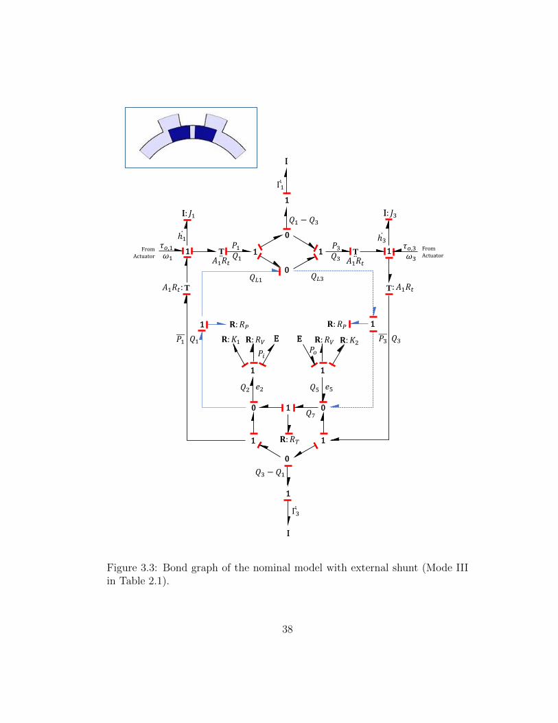
3.3 Bond graph of the nominal model with external shunt (ModeIII in Table 2.1). . . . . . . . . . . . . . . . . . . . . . . . . . 38
3.4 Block diagram for PID controller. . . . . . . . . . . . . . . . . 51
3.5 Block diagram for cascaded controller. . . . . . . . . . . . . . 58
4.1 Trajectories for control testing. . . . . . . . . . . . . . . . . . 61
4.2 First piston position and angular velocity states vs. time withPID control. . . . . . . . . . . . . . . . . . . . . . . . . . . . . 63
x
4.3 Second piston position and angular velocity states vs. time withPID control. . . . . . . . . . . . . . . . . . . . . . . . . . . . . 64
4.4 First piston position and angular velocity states vs. time withcascaded control. . . . . . . . . . . . . . . . . . . . . . . . . . 64
4.5 Second piston position and angular velocity states vs. time withcascaded control. . . . . . . . . . . . . . . . . . . . . . . . . . 65
4.6 Comparison of control inputs for the two control strategies. . . 65
4.7 Comparison of power consumed for the two control strategies. 66
4.8 Configuration space and phase plots for preliminary robustnesstesting (high-high). . . . . . . . . . . . . . . . . . . . . . . . . 69
4.9 Configuration space and phase plots for preliminary robustnesstesting (high-low). . . . . . . . . . . . . . . . . . . . . . . . . 69
4.10 Configuration space and phase plots for preliminary robustnesstesting (low-high). . . . . . . . . . . . . . . . . . . . . . . . . 70
4.11 Configuration space and phase plots for preliminary robustnesstesting (low-low). . . . . . . . . . . . . . . . . . . . . . . . . . 70
4.12 Comparison of control inputs for the two control strategies (high-high). . . . . . . . . . . . . . . . . . . . . . . . . . . . . . . . 71
4.13 Comparison of control inputs for the two control strategies (high-low). . . . . . . . . . . . . . . . . . . . . . . . . . . . . . . . . 71
4.14 Comparison of control inputs for the two control strategies (low-high). . . . . . . . . . . . . . . . . . . . . . . . . . . . . . . . 72
4.15 Comparison of control inputs for the two control strategies (low-low). . . . . . . . . . . . . . . . . . . . . . . . . . . . . . . . . 72
5.1 Synchronous trajectory provided by WCS [10]. . . . . . . . . . 76
5.2 States vs. time for first piston with PID control. . . . . . . . . 78
5.3 States vs. time for second piston with PID control. . . . . . . 78
5.4 States vs. time for first piston with cascaded control. . . . . . 79
5.5 States vs. time for second piston with cascaded control. . . . . 79
5.6 Comparison of control inputs for the two control strategies. . . 80
5.7 Comparison of power consumed for the two control strategies. 80
5.8 Configuration space design for optimal control formulation. . . 82
xi

Chapter 1
Introduction
Ventricular Assist Devices (VADs) are blood pumps that are designed
to support weak or failing hearts. The purpose of using VADs is to improve
blood circulation by creating an additional source of flow to the aorta from
the ventricle. VADs have increasingly become significant in bridge to recovery
or destination therapy considerations, with survival at about 80% at 1 year
and 70% at 2 years after implant. VADs have also been shown to be clinically
effective for patients waiting for a heart transplant, i.e., Bridge-to-Transplant
(BTT) [3, 15].
The Toroidal Ventricular Assist Device (TORVADTM) is a valveless,
positive-displacement pulsatile left-ventricular assist device (LVAD) designed
and developed by Windmill Cardiovascular Systems, Inc. (WCS, Inc., Austin,
TX). The TORVADTM can operate synchronized precisely to the timing of
the cardiac cycle using an epicardial ECG, and works by using two pistons
driven by independently controlled BLDC motors. Each piston is coupled to
each motor by a magnetic coupling across the titanium walls of the torus.
Pumping is then achieved by moving one piston within a toroidal pumping
chamber while the second piston is held between the inlet and the outlet ports
to occlude direct blood flow between the ports. As the first piston approaches
1

Figure 1.1: Working of the TORVADTM [8].
the completion of its cycle around the pumping chamber, the second piston
starts moving forward, thus inducing unidirectional pulsatile flow [8, 16, 26].
The working of the TORVADTM is shown in Fig. 1.1 [8]. The stages labeled
1–3 in Fig. 1.1 are the ‘driving’ phase, whereas 4–5 represent the ‘transition’
phase.
Fig. 1.2 [8] shows the connections between the left ventricle, the VAD
and the aorta. It should be noted that the pistons have the ability to travel
±3600 within the torus. For this reason, the motor positions must be precisely
monitored and controlled in order to prevent collisions and undesirable flow
conditions.
The control strategy currently used by WCS for controlling the posi-
tions of the pistons is to track a desired trajectory using a gain-scheduled PID
with feedforward terms. However, since a PID controller is purely based on
2

Figure 1.2: TORVADTM drawing blood from the left ventricle (right cannula)and providing flow into the left aorta (left cannula) [8].
the errors in the system, the controller for each motor is independent of the
other. The complex, non-linear fluid-mechanical coupling between the two
pistons must therefore be accounted for through judicious tuning of each set
of PID gains. It has been hypothesized that this fluid-mechanical coupling
is the cause of oscillations produced in the control voltages while the pistons
are controlled through the transition phase. A principal goal of this thesis
is to explore ways to model transition dynamics in the TORVADTM in order
to understand the aforementioned coupling effects and prove whether using
PID control leads to control oscillations, as well as explore other model-based
control methods and robustness of the same.
The modeling of the toroidal blood pump requires an understanding
3

of dynamics of the inertial fluid mass between the two pistons and changing
volumes. One way to deal with these effects is to treat the pump system as
an ‘open’ one, i.e., the fluid can enter and leave the system, and therefore, the
modeling of such systems is not trivial. Beaman and Breedveld [2] have shown
that it is possible to model such open systems without using active bonds,
controlled sources or other special artifacts. They proposed an energy analysis
to derive a bond graph model for open systems through the use of multiport
energy storage fields. The case studies presented by Beaman and Breedveld do
not investigate the scenario where there is a branch in the flow, as is the case
in the TORVADTM at the inlet and outlet ports. Similar analyses on open
systems have been presented by Redfield [22] and Cooke [4].
Margolis [19] presents an alternative method for modeling fluid systems
using bond graphs with a control volume analysis. However, this approach is
more applicable for compressible fluid dynamics, whereas the fluid flow in the
TORVADTM can be assumed to be incompressible. Margolis’ paper on the
modeling of two-stroke internal combustion engines using bond graphs [18]
also presents the model of a multi-energetic system, but does not incorporate
the simultaneous modeling of inertial variable-volume fluid elements and flow
branching effects. Shoureshi and McLaughlin [23] discuss the modeling of
incompressible fluid flow, but focus mainly on the thermodynamic aspects of
the systems.
The model of the blood pump presented in this thesis builds on the
framework proposed by Beaman and Breedveld [2] because their approach
4
takes into account the inertial variable-volume fluid elements as mentioned
before. Chapter 2 presents the model of the TORVADTM in detail by building
on the Beaman-Breedveld structure. Since the positions of the pistons relative
to the inlet/exit ports determine the direction of forces acting on the pistons, a
hybrid structure is proposed as it allows for efficient switching between modes
without introducing excessive complexity in the equations. Chapter 3 uses a
simplified nominal model and presents the design of a model-based cascaded
controller for the transition dynamics. The performance and preliminary ro-
bustness testing of this controller is compared with that of a PID controller
in Chapter 4. Conclusions drawn from this performance comparison are pre-
sented in Chapter 5, and areas for future work are also identified and presented
in that chapter.
5

Chapter 2
Multi-Energetic Pump Model
2.1 Components of the Multi-Energetic Model
The need for the development of a model of the two-piston toroidal
ventricular assist device has been discussed in Chapter 1. This chapter presents
the proposed model for characterizing transition dynamics in the pump.
Fig. 2.1 shows the pump under normal operating conditions during the
transition phase, which involves the two pistons exchanging their functional
roles. At the end of the transition phase, piston ‘1’ will be held in the ‘trap’, the
region between the inlet and outlet ports, whereas piston ‘2’ will be driven in
the torus according to a desired trajectory. A hybrid model is used to represent
the different modes of the pump according to the different relative positions
of the pistons. A hybrid model allows the system to be represented using
separate modes of operation of the pump as opposed to using a single complex
model, and therefore, the dynamic equations for each mode do not include
effects that are not active, i.e., the modes do not include model elements that
do not transfer, store or dissipate significant levels of energy. This allows the
equations representing the dynamics of each mode to take a simpler form when
compared to the single model. For a model-based control design, as presented
in Chapter 3, the hybrid structure is beneficial as the computational load is
6

2
𝑄2 𝑄5
𝜃3, 𝜔3, 𝑄3
Trap
Figure 2.1: Schematic of the toroidal blood pump in the ‘approach’ phase(Mode I in Table 2.1).
reduced due to the simpler hybrid model dynamics formulation mentioned
above.
In the schematic shown in Fig. 2.1, Q1 and Q3 are the volumetric flow
rates generated by the pistons, and Q2 and Q5 are the exit and entry flow
rates, respectively. The constituent components of the model of the pump are
discussed below, and a complete hybrid model is presented in the next section.
2.1.1 Modified Beaman-Breedveld Structure
The concepts and techniques used to develop the model are derived
from the ideal case studies presented by Beaman and Breedveld [2] in their
study to demonstrate the use of bond graphs for modeling open and closed
physical systems with incompressible fluid flow. In their paper, Beaman and
7
Figure 2.2: Fluid modeled as multi-port I-junction [2].
Breedveld use multi-port bond graph elements to capture the energy storage
properties of the fluid due to fluid flow and changing volume respectively. The
Beaman-Breedveld structure showing this multi-port I-junction [14] is shown
in Fig. 2.2. This multi-port formulation only represents the stored energy in
the fluid due to the kinetic energy of the contained fluid.
In the toroidal pump, there is inflow of fluid at the inlet port, and
outflow of fluid at the exit port, and hence, the fluid masses on either side of
a piston have to be treated as open systems, i.e., systems in which there is
an exchange of matter with the environment. Therefore, a similar structure
is used in the pump model for the fluid with changing volume. The Beaman-
Breedveld structure is extended here to model a division in fluid flow that
might occur if there is an exit flow coupled with a changing volume fluid mass.
Such a scenario can be observed at the ports of the pump if the fluid on either
side of a piston is considered to have inertial properties. In addition to the
assumptions made earlier, it is assumed that the energy stored in the fluid
8
depends on the relative fluid flow rate generated by the motion of the two
pistons, Q1 − Q3. This is because if one of the pistons is considered to be
fixed while the other is being driven around the torus, then the contained
fluid volume has a flow rate that is equal to the relative volumetric flow rate.
Note that when both the pistons are moving at the same velocity (Q1 = Q3),
it can be seen that any energy stored due to the momentum of the fluid
volume is zero as the relative volumetric flow rate is zero, Q1 −Q3 = 0. This
condition holds true in a steady state because the piston velocities are equal,
the corresponding volumetric flow rates are constant, and the inertial pressure
of the fluid would not affect the control voltages required to drive the pistons.
In such a steady state, only the resistive elements in the model affect these
control voltages. This model, however, would fail to include inertial effects
of the fluid volume when the relative volumetric flow rate is zero but the
system is not in steady state, i.e., both the pistons are accelerating but their
respective velocities are the same. Therefore, in such a case, the proposed
model would not completely capture the desired effects. However, such cases
occur rarely during the normal operation of the pump, because in the driving
phase, one of the pistons is held fixed in the ‘trap’, whereas in the transition
phase, the pistons are either driven in steady state or at different velocities,
and therefore, the time for which the unaccounted inertia affects the model
accuracy is minimal. It is to be noted that this hybrid model is designed for
the purpose of understanding the dynamics of the pump in its normal modes of
operation, during which the assumptions made above hold true, and therefore,
9

is not a general model. If such a model is to be constructed that can be used
to represent the pump irrespective of its mode of operation, the assumption
regarding the dependence of energy stored in the fluid masses on the relative
volumetric flow rates does not hold true for all cases, and therefore, separate
assumptions have to be made.
Since there is some power going out of the system from the exit port
because of the fluid flow, Q2, a parallel path is established that is used to
balance the flow at the junction. QL1 and QL3 are leakage flows across the
first and the second piston respectively. These flows exist because of the gap
between the torus walls and the pistons. The other elements attached to
this parallel path are the static pressure at the port, the dynamic pressure
generated due to the fluid flow [11] and the resistance due to valving, which
will be discussed later.
The modified Beaman-Breedveld structure for the outlet port is pre-
sented in bond graph form in Fig. 2.3. In this structure, the blue dotted bonds
represent the parallel leakage flow across the pistons, whereas the black solid
bonds represent power transfer through the primary fluid flow. The top half
of the branch in the primary flow shows the energy stored in the fluid, whereas
the bottom half represents the fluid flow balance equation at the junction.
The equations for the changing fluid inertia model can be derived from
10
T 𝐴1𝑅𝑡
𝑃1𝑄1
1
𝑒1
0
0
I
𝑄1 − 𝑄3
1
Γ1
1
0G 1
𝑉1
1 T 𝐴1𝑅𝑡
𝑃3𝑄3
1
𝐑:𝑅𝑉
𝑒2𝑄2
𝑃𝑜
E𝐑:𝐾1
𝑄𝐿1 𝑄𝐿3
Figure 2.3: Modified Beaman-Breedveld structure.
the bond graph as follows:
Γ1 =ρV1(Q1 −Q3)
A21
(2.1)
E1 =A2
1Γ21
2ρV1
(2.2)
eΓ1(Q1 −Q3) =∂E1
∂Γ1
Γ1 +∂E1
∂V1
V1 (2.3)
e1 =∂E1
∂V1
(2.4)
V1 = Q3 −Q1 (2.5)
Q1 +QL1 = Q2 +Q3 +QL3 (2.6)
where Γ1 is the generalized fluid momentum, ρ is the density of the fluid, V1
11

is the volume of the fluid mass, A1 is the flow area, Q1 and Q3 are volumetric
flow rates generated by the motion of the pistons, and E1 is the kinetic energy
stored in the fluid. Equation (2.6) shows the balance of fluid flow at the
junction.
2.1.2 Loss Models
The various loss effects that have been incorporated into the model
of the pump will now be described. For the leakage flow across the pistons,
the pressure drop across the pistons can be related to the flow through a
rectangular cross-section (annular), and therefore, a resistive element can be
used to represent this effect in the bond graph. Equations (2.7)–(2.8) show
the resistance model [27], where fD is the Darcy friction factor, L is the length
of the pipe, ∆P is the pressure drop, Q is the flow rate, D is the hydraulic
diameter, A is cross-section area and P is the wetted perimeter. The resistance
due to flow along the toroidal rectangular tube can also be modeled using the
same structure, but with a different hydraulic diameter. However, the pressure
difference due to resistance to flow in the torus is negligible compared to the
pressure difference generated due to leakage.
∆P
L= fD
ρ
2D
(Q
A
)2
(2.7)
D =4A
P(2.8)
The valving at the ports can also be modeled as flow through a rect-
angular orifice, and can similarly be represented in the bond graph as another
12
resistive element, characterized by the equation (2.9) [27]. However, it has to
be noted that the direction of pressure drop changes with the direction of flow.
In this case, ∆P is the generated pressure differential, A is the flow area, and
Q is the volumetric flow rate across the valve.
Q = gA√|∆P | (2.9)
g = 0.7
√2
ρ(2.10)
The resistance due to the shear of the fluid (solid-fluid interaction) is
also included in the model. It can be represented by equation (2.11) [27]. FR
is the resistive force acting on the piston if the fluid viscosity is µ, the face
area of the piston is Ap,s, the piston velocity is v, and the gap between the
piston and the tube wall is d.
FR =µAp,sv
d(2.11)
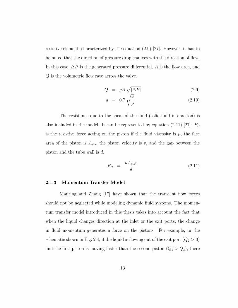
2.1.3 Momentum Transfer Model
Manring and Zhang [17] have shown that the transient flow forces
should not be neglected while modeling dynamic fluid systems. The momen-
tum transfer model introduced in this thesis takes into account the fact that
when the liquid changes direction at the inlet or the exit ports, the change
in fluid momentum generates a force on the pistons. For example, in the
schematic shown in Fig. 2.4, if the liquid is flowing out of the exit port (Q2 > 0)
and the first piston is moving faster than the second piston (Q1 > Q3), there
13
2
𝑄2 𝑄5
𝜃3, 𝜔3, 𝑄3
Change in fluid momentum
Tangential force acting on piston
Figure 2.4: Schematic of momentum transfer model.
is a force acting on the second piston in the positive direction due to the direc-
tional change in fluid momentum. However, this momentum transfer model
is not required if either port is closed, i.e., there is no liquid flowing in or out
of the system. This is justified by the fact that when there is no fluid flow
through the ports, there is no direction change in the fluid flow, thus making
the momentum transfer model unnecessary. The momentum transfer model
does not include the effect of flow due to leakage, which can be justified by the
fact that the leakage flow is generally negligible compared to the primary flow,
and that the leakage is symmetric, and therefore the forces generated cancel
each other.
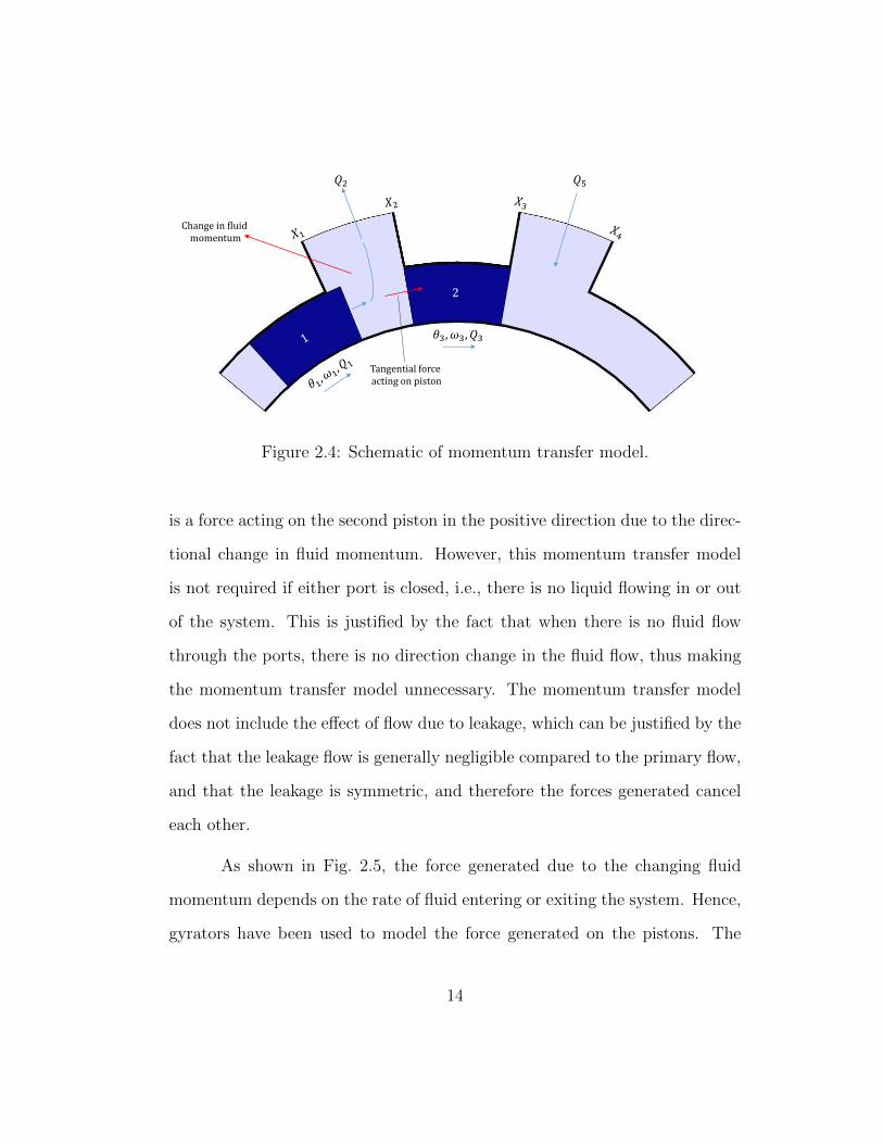
As shown in Fig. 2.5, the force generated due to the changing fluid
momentum depends on the rate of fluid entering or exiting the system. Hence,
gyrators have been used to model the force generated on the pistons. The
14
1𝜏𝑜,1𝜔1
I: 𝐽1
T 𝐴1𝑅𝑡
𝑃1𝑄1
1
0
0
𝑄1 − 𝑄3
ℎ1
1 T 𝐴1𝑅𝑡
𝑃3𝑄3
1
I: 𝐽3
𝜏𝑜,3𝜔3
From Actuator
FromActuator
TT𝐴1𝑅𝑡: : 𝐴1𝑅𝑡
1
𝐑:𝑅𝑉
𝑒2𝑄2
𝑃𝑜
E𝐑:𝐾1
G G∙∙∙∙
𝜐1𝛾2𝑅𝑡−𝜂1𝛾2𝑅𝑡
Inertial Fluid Model
Figure 2.5: Bond graph of momentum transfer model.
variable γ2 represents the fluid momentum per unit volume, and η1 and ν1 are
activation variables whose values are dependent on the direction of the flow
into or out of the port. It is to be noted that other components of the bond
graph have been removed from Fig. 2.5 for simplicity.
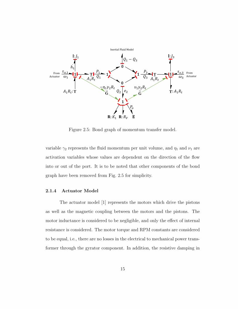
2.1.4 Actuator Model
The actuator model [1] represents the motors which drive the pistons
as well as the magnetic coupling between the motors and the pistons. The
motor inductance is considered to be negligible, and only the effect of internal
resistance is considered. The motor torque and RPM constants are considered
to be equal, i.e., there are no losses in the electrical to mechanical power trans-
former through the gyrator component. In addition, the resistive damping in
15
𝑉
𝐑:𝑅
𝑖
𝐾𝑇
1
I: 𝐽𝑚
𝑖
𝜏𝑚𝜔𝑚
0
C: 𝐾𝑐
𝜏𝑜𝜔𝑚 𝜔
ℎ𝑚To Piston1 GE
𝑉𝑏
Figure 2.6: Bond graph of actuator model with magnetic coupling.
the magnetic coupling between the motor and the piston is considered to be
negligible. The actuator bond graph structure is shown in Fig. 2.6.
The equations governing the actuator model are shown below:
E = iR + Vb (2.12)
τo = Kc(θm − θ) (2.13)
hm = τm − τ0 (2.14)
τm = KT i (2.15)
Vb = KTωm (2.16)
i =E −KTωm
R(2.17)
where E is the input voltage, KT is the motor torque constant (equal to the
RPM constant), Kc is the coupling stiffness, and i and R are the motor current
and internal resistance respectively. θ and θm are the positions of the centres
of the piston and the motor respectively, and hm is the angular momentum of
the motor.
16

2.2 Complete Fluid Model and State Equations
The various components discussed in Section 2.1 can be put together
to construct the bond graph model for the toroidal blood pump. This section
presents the bond graph and the corresponding state equations for the mode of
operation shown in Fig. 2.1, i.e., the ‘approach’ phase. In this mode, piston ‘1’
is approaching the trap and piston ‘2’ is held in the trap. Since a hybrid model
is proposed, the models for the other modes of operation will be discussed in
the next section.
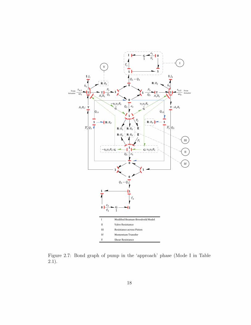
2.2.1 Bond Graph Structure of the Pump
The bond graph for the ‘approach’ phase is shown in Fig. 2.7. The
different constituent components are also labeled in Fig. 2.7.
17
1𝜏𝑜,1𝜔1
I: 𝐽1
T 𝐴1𝑅𝑡
𝑃1
𝑄1
1
𝑒1
0
0
I
𝑄1 − 𝑄3
1
Γ1
1
0G 1 𝑉1
ℎ1
1 T 𝐴1𝑅𝑡
𝑃3
𝑄3
1
I: 𝐽3
𝜏𝑜,3𝜔3
From Actuator
FromActuator
TT𝐴1𝑅𝑡: : 𝐴1𝑅𝑡
1
𝐑:𝑅𝑉
1
0
0
1
𝑃3 𝑄3
1
1
𝐑:𝑅𝑉
𝑃1 𝑄1
𝑄3 − 𝑄1
𝑒2
𝑒5
𝑄2
𝑄5
I
Γ3
1
0 G 1 𝑉3
𝑒3
1 1𝐑:𝑅𝑃𝐑:𝑅𝑃
𝑃𝑜
E
E
𝑃𝑖
𝐑:𝐾1
𝐑:𝐾2
𝐑:𝑅𝑆 𝐑:𝑅𝑆
II
I
III
GG : 𝜐2𝛾5𝑅𝑡−𝜂2𝛾5𝑅𝑡:
G
IV
V
G∙∙∙∙
𝜐1𝛾2𝑅𝑡−𝜂1𝛾2𝑅𝑡
𝑄𝐿3
ℎ3
𝑄𝐿1
I Modified Beaman-Breedveld Model
II Valve Resistance
III Resistance across Piston
IV Momentum Transfer
V Shear Resistance
Figure 2.7: Bond graph of pump in the ‘approach’ phase (Mode I in Table2.1).
18

2.2.2 Model States and Equations
From the bond graph, the intermediate equations governing the system
can be derived. These relations are shown below:
V1 = (θ3 − θ1 − θL)HtR2to −R2
ti
2(2.18)
V3 = (2π + θ1 − θ3 − θL)HtR2to −R2
ti
2(2.19)
Q1 = ω1A1Rt (2.20)
Q3 = ω3A1Rt (2.21)
e1 = −ρ2
(Q1 −Q3
A1
)2
(2.22)
e3 = −ρ2
(Q3 −Q1
A1
)2
(2.23)
QL3 = −QL1 (2.24)
Q5 = Q2 (2.25)
Pdiff = Pout − Pin +
(1 +
sgn(Q2)
0.49
)ρ
2(Q2/(A2f1))2 (2.26)
−(
1− sgn(Q2)
0.49
)ρ
2(Q2/(A2f2))2
QL1 = −PdiffKR,p
(2.27)
Q2 = Q1 −Q3 + 2QL1 (2.28)
γ2 = ρ|Q2|A2f1
(2.29)
γ5 = ρ|Q5|A2f2
(2.30)
e2 = Pout +
(1 +
sgn(Q2)
0.49
)ρ
2(Q2/(A2f1))2 (2.31)
e5 = Pin +
(1− sgn(Q2)
0.49
)ρ
2(Q2/(A2f2))2 (2.32)
19
where V1 and V3 are the volumes of the fluid blocks in the pump, θL is the
angle swept by the pistons, Rto and Rti are the outer and inner radii of the
torus, KR,p is the resistance across the pistons defined by equation (2.7), Ht is
the torus channel height, and f1 and f2 are the fractions of the exit and inlet
ports respectively, representing how much each port is open as a fraction of the
total area of the port, A2. It can be seen that due to an algebraic loop in the
equations, a set of non-linear equations have to be solved to find the values of
Q2 andQL1. This algebraic loop can be shown in the bond graph if the dynamic
pressure due to the exiting/entering kinetic energy of the fluid is modeled
as a constant effort source with a resistive element connected to it, which
makes the causal structure of the graph indeterminate. The contribution of the
momentum transfer forces is considered to be negligible in the aforementioned
non-linear equations for simplicity. As a result, the momentum transfer terms
are only present in the dynamic equations.
The fractions f1 and f2 can be written as:
f1 =
1 if θ1 < X1 − θL/2X2−θ1−θL/2
θ`if θ1 ≥ X1 − θL/2 and θ1 < X2 − θL/2
(2.33)
f2 =
1 if θ3 < X3 − θL/2X4−θ3−θL/2
θ`if θ3 ≥ X3 − θL/2 and θ3 < X4 − θL/2
(2.34)
where X2 and X4 are the positions of the ports on the pump as shown in Fig.
2.1, and θ` is the angle swept by the input/output ports.
Using equations (2.18)–(2.32), the differential dynamic equations gov-
20
erning the system can be defined as:
θ1 = h1/J (2.35)
θ3 = h3/J (2.36)
h1 = τo,1 −KR,sω1 − P1A1Rt + P1A1Rt + η1γ2Q2Rt (2.37)
−η2γ5Q5Rt
= τo,1 −KR,sω1 −(e2 + Γ1 − e1 + ν1γ2ω3Rt (2.38)
−η1γ2ω1Rt
)A1Rt +
(e5 + Γ3 − e3 + ν2γ5ω3Rt
−η2γ5ω1Rt
)A1Rt + η1γ2Q2Rt − η2γ5Q5Rt
h3 = τo,3 −KR,sω3 + P3A1Rt − P3A1Rt + ν1γ2Q2Rt (2.39)
−ν2γ5Q5Rt
= τo,3 −KR,sω3 +(e2 + Γ1 − e1 + ν1γ2ω3Rt (2.40)
−η1γ2ω1Rt
)A1Rt −
(e5 + Γ3 − e3 + ν2γ5ω3Rt
−η2γ5ω1Rt
)A1Rt + ν1γ2Q2Rt − ν2γ5Q5Rt
θ1m = h1m/Jm (2.41)
θ3m = h3m/Jm (2.42)
h1m = τ1m − τo,1 (2.43)
h3m = τ3m − τo,3 (2.44)
where τo,1 and τo,3 are the torque inputs coming into the system from the
actuator model, τ1m and τ3m can be determined from the actuator model with
voltage as input, and KR,s is the resistance due to shear (with the torque
conversion multiplier), as discussed in equation (2.11). The values of η (ν) are
21

activated only when Q2 < 0 (> 0). It is interesting to note that the terms
Γ1 and Γ3 contain both Q1 and Q3, and thus, a simultaneous equation has
to be solved to separate h1 and h3. This is because of the dependent causal
structure in the bond graph.
Hence, for the pump model with actuators, the different states can be
characterized by the state vector X ∈ R8:
X = [θ1 θ3 h1 h3 θ1m θ3m h1m h3m]T
The state variables are defined as follows:
• θ1: Angular position of the first piston [rad]
• θ3: Angular position of the second piston [rad]
• h1: Angular momentum of the first piston [kg-m2/s]
• h3: Angular momentum of the second piston [kg-m2/s]
• θ1m: Angular position of the first motor [rad]
• θ3m: Angular position of the second motor [rad]
• h1m: Angular momentum of the first motor [kg-m2/s]
• h3m: Angular momentum of the second motor [kg-m2/s]
The control inputs to the system are the two voltages provided to the
motors, and can be characterized by the state vector U ∈ R2:
U = [E1 E3]T
22
where E1 [V] and E3 [V] are the voltages supplied to the first and the second
motor respectively.
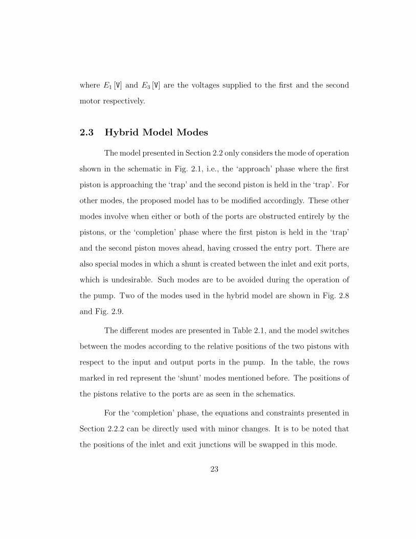
2.3 Hybrid Model Modes
The model presented in Section 2.2 only considers the mode of operation
shown in the schematic in Fig. 2.1, i.e., the ‘approach’ phase where the first
piston is approaching the ‘trap’ and the second piston is held in the ‘trap’. For
other modes, the proposed model has to be modified accordingly. These other
modes involve when either or both of the ports are obstructed entirely by the
pistons, or the ‘completion’ phase where the first piston is held in the ‘trap’
and the second piston moves ahead, having crossed the entry port. There are
also special modes in which a shunt is created between the inlet and exit ports,
which is undesirable. Such modes are to be avoided during the operation of
the pump. Two of the modes used in the hybrid model are shown in Fig. 2.8
and Fig. 2.9.
The different modes are presented in Table 2.1, and the model switches
between the modes according to the relative positions of the two pistons with
respect to the input and output ports in the pump. In the table, the rows
marked in red represent the ‘shunt’ modes mentioned before. The positions of
the pistons relative to the ports are as seen in the schematics.
For the ‘completion’ phase, the equations and constraints presented in
Section 2.2.2 can be directly used with minor changes. It is to be noted that
the positions of the inlet and exit junctions will be swapped in this mode.
23

Figure 2.8: Schematic of the toroidal blood pump with an obstructed port(Mode VIII in Table 2.1).
𝑄2 𝑄5
Bypass Path
Figure 2.9: Schematic of the toroidal blood pump with an internal shunt (ModeVII in Table 2.1).
24

Table 2.1: Modes for hybrid model.Mode Piston 1 Piston 2I (Approach) Left of Exit Port TrapII Blocking Exit Port TrapIII Trap TrapIV Left of Exit Port Blocking Entry PortV Blocking Exit Port Blocking Entry PortVI Trap Blocking Entry PortVII Left of Exit Port Right of Entry PortVIII Blocking Exit Port Right of Entry PortIX (Completion) Trap Right of Entry Port
The rationale behind choosing a hybrid model to represent the system
has been presented in Section 2.1. However, care has to be taken to ensure
the conservation of total energy contained in the system across modes. The
assumption made earlier that the kinetic energy stored in the fluid depends on
the relative flow rate generated by piston motion guarantees energy conserva-
tion across modes if the angular velocities of the pistons are consistent when
switching between modes.
2.3.1 Modes with Obstructed Ports
When either one of the ports is completely blocked off by a piston
(Fig. 2.8), the model becomes simpler because of many reasons. Firstly, the
algebraic loop in the kinematic equations is no longer present because there can
be no fluid exiting or entering the system in this state, and thus, the dynamic
pressures are not present. Secondly, the momentum transfer terms are also
absent since there is no fluid momentum entering or escaping the system.
25

Finally, the leakage flow rates can easily be calculated from the difference in
the primary flow rates generated by the pistons because of a change in causal
structure in the model. The modified equations can be written as follows:
QL3 = −QL1 (2.45)
Q5 = Q2 (2.46)
QL1 = −Q1 −Q3
2(2.47)
Q2 = Q1 −Q3 + 2QL1
= 0 (2.48)
e2 = −KR,pQL1 + Pin (2.49)
e5 = Pin (2.50)
θ1 = h1/J (2.51)
θ3 = h3/J (2.52)
h1 = τo,1 −KR,sω1 − P1A1Rt + P1A1Rt (2.53)
= τo,1 −KR,sω1 −(e2 + Γ1 − e1
)A1Rt (2.54)
+(e5 + Γ3 − e3
)A1Rt
h3 = τo,3 −KR,sω3 + P3A1Rt − P3A1Rt (2.55)
= τo,3 −KR,sω3 +(e2 + Γ1 − e1
)A1Rt (2.56)
−(e5 + Γ3 − e3
)A1Rt
θ1m = h1m/Jm (2.57)
θ3m = h3m/Jm (2.58)
26
h1m = τ1m − τo,1 (2.59)
h3m = τ3m − τo,3 (2.60)
It has to be noted that a part of the leakage flow may enter or exit the
pump, but this flow is minimal, and therefore, can be neglected. Hence, the
system is considered to be closed in these modes.
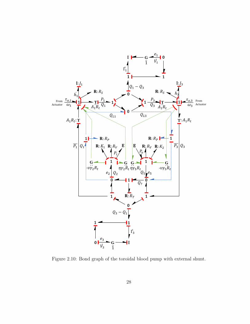
2.3.2 Modes with Shunts
As mentioned before, a shunt is not desirable as the fluid can flow back
from the high pressure output port to the low pressure input port if there is
no piston directly obstructing the backward flow path of the fluid. However,
the desired trajectory can force the system into such a position. This may
happen in two modes – when both the pistons are in the ‘trap’, leading to
shunt around the torus (external shunt), and when the pistons are outside the
‘trap’, leading to an internal shunt. Fig. 2.9 is a visual representation of the
internal shunt. These two modes are also presented in Table 2.1 (Modes III
and VII).
For these modes, the bond graph for the model has to be modified in
order to capture the change in effect. The modified bond graph for the external
shunt mode is shown in Fig. 2.10. The internal shunt mode can be similarly
modeled.
It has to be noted that if there is a shunt, the resistance due to the torus
flow, which was considered to be negligible in other modes, has to be accounted
27
1𝜏𝑜,1𝜔1
I: 𝐽1
T 𝐴1𝑅𝑡
𝑃1𝑄1
1
𝑒1
0
0
I
𝑄1 − 𝑄3
1
Γ1
1
0G 1
𝑉1
ℎ1
1 T 𝐴1𝑅𝑡
𝑃3𝑄3
1
I: 𝐽3
𝜏𝑜,3𝜔3
From Actuator
FromActuator
TT𝐴1𝑅𝑡: : 𝐴1𝑅𝑡
1
0
0
1
𝑃3 𝑄3
1
1
𝐑:𝑅𝑉𝑃1 𝑄1
𝑄3 − 𝑄1
𝑒5𝑄5
I
Γ3
1
0 G 1
𝑉3
𝑒3
1 1𝐑:𝑅𝑃𝐑:𝑅𝑃
E𝑃𝑜
𝐑:𝐾2
𝐑:𝑅𝑆 𝐑:𝑅𝑆
GG
-𝜐𝛾5𝑅𝑡-𝜐𝛾2𝑅𝑡
10
1
𝑒2 𝑄2
𝐑:𝑅𝑉 E𝐑:𝐾1
𝑃𝑖
𝑄7
𝑄𝐿3𝑄𝐿1
. . . .G
𝜂𝛾5𝑅𝑡. .G
𝜂𝛾2𝑅𝑡. .
𝐑: 𝑅𝑇
ℎ3
Figure 2.10: Bond graph of the toroidal blood pump with external shunt.
28

for in order for the model to have a proper causal structure. Therefore, an
extra resistance due to the torus, KR,t, has to be introduced. However, the
main resistive element is still that due to the valving effect created due to
the pistons obstructing the input/output ports. Additionally, the flow in the
torus is also represented by a new variable, Q7. As in equations (2.18)–(2.32),
the momentum transfer terms are considered to be negligible in the set of
non-linear constraint equations to solve for QL1, Q2 and Q7.
The equations governing the toroidal pump in such a mode can be
written as:
Pdiff = Pout − Pin +
(1 +
sgn(Q2)
0.49
)ρ
2(Q2/(A2f1))2 (2.61)
−(
1− sgn(Q2)
0.49
)ρ
2(Q2/(A2f2))2
QL1 =Q3 −Q1
2+Pdiff2KR,p
(2.62)
Q7 =PdiffKR,t
(2.63)
Q2 = Q7 −Q1 −QL1 (2.64)
QL3 = QL1 − (Q3 −Q1) (2.65)
Q5 = Q2 (2.66)
e2 = Pout +
(1 +
sgn(Q2)
0.49
)ρ
2(Q2/(A2f1))2 (2.67)
e5 = Pin +
(1− sgn(Q2)
0.49
)ρ
2(Q2/(A2f2))2 (2.68)
ej = e2 −KR,pQL1 (2.69)
29
θ1 = h1/J (2.70)
h1 = τo,1 −KR,sω1 − P1A1Rt + P1A1Rt (2.71)
= τo,1 −KR,sω1 −(ej + Γ1 − e1
)A1Rt (2.72)
+(e2 + Γ3 − e3 + (η + ν)γ2ω1Rt
)A1Rt + (η − ν)γ2Q2Rt
θ3 = h3/J (2.73)
h3 = τo,3 −KR,sω3 + P3A1Rt − P3A1Rt (2.74)
= τo,3 −KR,sω3 +(ej + Γ1 − e1
)A1Rt (2.75)
−(e5 + Γ3 − e3 + (η + ν)γ5ω3Rt)
)A1Rt − (η − ν)γ5Q5Rt
θ1m = h1m/Jm (2.76)
h1m = τ1m − τo,1 (2.77)
θ3m = h3m/Jm (2.78)
h3m = τ3m − τo,3 (2.79)
In the modes with shunts, the activation variables for the momentum
transfer model are different from those presented in Section 2.2.2, and can be
written as:
η =
1 if Q2 > 0 and Q7 > 0
0 otherwise(2.80)
ν =
1 if Q2 < 0 and Q7 < 0
0 otherwise(2.81)
30
2.4 Summary
This chapter focused on the construction of a hybrid model for the
toroidal blood pump for characterization of transition dynamics. Constituent
components of the model were discussed, and modes of operation of the pump
were also presented. The proposed model will be used in the following chapter
to design a control strategy for trajectory tracking during the transition phase.
The hybrid model for the pump will also be used in Chapter 4 to
generate simulation results to compare the performance of the designed model-
based control strategy against that of a PID control strategy.
31
Chapter 3
Control Strategies for Transition Dynamics
3.1 Simplified Model for Controller Design
Now that a hybrid model of the toroidal blood pump has been devel-
oped, this model can be used for testing various control strategies for trajectory
tracking. This chapter addresses the various requirements for control design
using both error-based and model-based approaches.
The first step towards designing the controller is the development of a
nominal plant model which simplifies the system without compromising on the
key elements in the dynamic model to allow for real-time computation. This
so-called ‘simplified’ nominal plant model can then be used for designing the
required observers for state feedback and model-based control applications.
This section presents the nominal plant models for different modes in the two-
piston toroidal blood pump.
3.1.1 Nominal Models for Normal Operating Conditions
The nominal plant model for the pump in the ‘approach’ phase (Mode I
in Table 2.1) is presented in Fig. 3.1. A similar nominal model can also be used
for the ‘completion’ phase with minor changes as shown in Chapter 2. The
nominal model for the pump when the exit port is obstructed by the piston
32
(Mode II in Table 2.1) is shown in Fig. 3.2. All other modes with obstructed
ports can be similarly modeled.
It is evident from Fig. 3.1 and Fig. 3.2 that the nominal models elimi-
nate any dynamic pressures present in the actual models, and therefore there
are no algebraic loops remaining as the causally indeterminate part of the
pump model is removed. It is also assumed that the momentum transfer effect
is not a significant contributing factor because of the small face area of the
pistons, and therefore, momentum transfer components are not included in the
nominal plant model. It is shown later, in Chapter 4, that the performance
of the model-based controller is not compromised in terms of tracking perfor-
mance in spite of this assumption. The effects of valving and shear resistances
are also considered to be negligible, and therefore, these resistances are also
eliminated. No additional assumptions are made in the actuator model.
The intermediate and state equations for each nominal plant model can
be derived from the bond graphs. For the ‘approach’ phase, the equations are
as follows:
V1 = (θ3 − θ1 − θL)HtR2to −R2
ti
2(3.1)
V3 = (2π + θ1 − θ3 − θL)HtR2to −R2
ti
2(3.2)
Q1 = ω1A1Rt (3.3)
Q3 = ω3A1Rt (3.4)
e2 = Pout (3.5)
e5 = Pin (3.6)
33
1𝜏𝑜,1𝜔1
I: 𝐽1
T 𝐴1𝑅𝑡
𝑃1𝑄1
1
0
0
I
𝑄1 − 𝑄3
1
Γ1
ℎ1
1 T 𝐴1𝑅𝑡
𝑃3𝑄3
1
I: 𝐽3
𝜏𝑜,3𝜔3
From Actuator
FromActuator
TT𝐴1𝑅𝑡: : 𝐴1𝑅𝑡
1
1
0
0
1
𝑃3 𝑄3
1
1
𝑃1 𝑄1
𝑄3 − 𝑄1
𝑒2
𝑒5
𝑄2
𝑄5
I
Γ3
1 1𝐑:𝑅𝑃𝐑:𝑅𝑃 𝑃𝑜
E
E𝑃𝑖
𝑄𝐿3𝑄𝐿1
ℎ3
Figure 3.1: Bond graph of the nominal model in the ‘approach phase’ (ModeI in Table 2.1).
34
1𝜏𝑜,1𝜔1
I: 𝐽1
T 𝐴1𝑅𝑡
𝑃1𝑄1
1
0
0
I
𝑄1 − 𝑄3
1
Γ1
ℎ1
1 T 𝐴1𝑅𝑡
𝑃3𝑄3
1
I: 𝐽3
𝜏𝑜,3𝜔3
From Actuator
FromActuator
TT𝐴1𝑅𝑡: : 𝐴1𝑅𝑡
1
0
0
1
𝑃3 𝑄3
1
1
𝑃1 𝑄1
𝑄3 − 𝑄1
𝑒5𝑄5
I
Γ3
1 1𝐑:𝑅𝑃𝐑:𝑅𝑃
E𝑃𝑖
𝑄𝐿3𝑄𝐿1
ℎ3
Figure 3.2: Bond graph of the nominal model with obstructed exit port (ModeII in Table 2.1).
35
θ1 = h1/J (3.7)
θ3 = h3/J (3.8)
h1 = τo,1 − P1A1Rt + P1A1Rt (3.9)
= τo,1 −(e2 + Γ1
)A1Rt +
(e5 + Γ3
)A1Rt (3.10)
h3 = τo,3 + P3A1Rt − P3A1Rt (3.11)
= τo,3 +(e2 + Γ1
)A1Rt −
(e5 + Γ3
)A1Rt (3.12)
θ1m = h1m/Jm (3.13)
θ3m = h3m/Jm (3.14)
h1m = τ1m − τo,1 (3.15)
h3m = τ3m − τo,3 (3.16)
The equations for the ‘completion’ phase can be similarly derived. For
the modes with obstructed ports, the state equations (3.7)–(3.16) hold, and
there are minor changes for the constraints as shown (with Mode II from Table
2.1 as example):
V1 = (θ3 − θ1 − θL)HtR2to −R2
ti
2(3.17)
V3 = (2π + θ1 − θ3 − θL)HtR2to −R2
ti
2(3.18)
Q1 = ω1A1Rt (3.19)
Q3 = ω3A1Rt (3.20)
QL1 =Q3 −Q1
2(3.21)
e2 = −KR,pQL1 + Pin (3.22)
e5 = Pin (3.23)
36

3.1.2 Nominal Model for Shunt Cases
The special cases with shunts have to be dealt with more carefully.
This is because the valving resistances and the dynamic pressures due to in-
put/output flow may be significant compared to other efforts in the model, and
therefore, cannot be neglected. The dynamic pressures due to the changing
volumes of the inertial fluid elements, the shear resistances, and the momen-
tum transfer effect are eliminated as in the other nominal models. The nominal
model for the external shunt case is shown in Fig. 3.3.
The dynamic pressures and the valving resistances in the nominal model
create an algebraic loop, as in the actual plant model. Assuming that there
will always be reversed flow in these modes (Q2 < 0) makes the non-linear
simultaneous equations easy to solve, as it removes the non-linearities due to
the signum function. The equations for the nominal model in the case of an
external shunt become:
Pdiff = Pout − Pin +
(1− 1
0.49
)ρ
2(Q2/(A2f1))2 (3.24)
−(
1 +1
0.49
)ρ
2(Q2/(A2f2))2
QL1 =Q3 −Q1
2+Pdiff2KR,p
(3.25)
Q7 =PdiffKR,t
(3.26)
Q2 = Q7 −Q1 −QL1 (3.27)
QL3 = QL1 − (Q3 −Q1) (3.28)
37
1𝜏𝑜,1𝜔1
I: 𝐽1
T 𝐴1𝑅𝑡
𝑃1𝑄1
1
0
0
I
𝑄1 − 𝑄3
1
Γ1
ℎ1
1 T 𝐴1𝑅𝑡
𝑃3𝑄3
1
I: 𝐽3
𝜏𝑜,3𝜔3
From Actuator
FromActuator
TT𝐴1𝑅𝑡: : 𝐴1𝑅𝑡
1
0
0
1
𝑃3 𝑄3
1
1
𝐑:𝑅𝑉𝑃1 𝑄1
𝑄3 − 𝑄1
𝑒5𝑄5
I
Γ3
1 1𝐑:𝑅𝑃𝐑:𝑅𝑃
E𝑃𝑜
𝐑:𝐾2
10
1
𝑒2𝑄2
𝐑:𝑅𝑉 E𝐑:𝐾1
𝑃𝑖
𝑄7
𝑄𝐿3𝑄𝐿1
𝐑:𝑅𝑇
ℎ3
Figure 3.3: Bond graph of the nominal model with external shunt (Mode IIIin Table 2.1).
38
Q5 = Q2 (3.29)
e2 = Pout +
(1− 1
0.49
)ρ
2(Q2/(A2f1))2 (3.30)
e5 = Pin +
(1 +
1
0.49
)ρ
2(Q2/(A2f2))2 (3.31)
ej = e2 −KR,pQL1 (3.32)
θ1 = h1/J (3.33)
h1 = τo,1 − P1A1Rt + P1A1Rt (3.34)
= τo,1 −(ej + Γ1
)A1Rt +
(e2 + Γ3
)A1Rt (3.35)
θ3 = h3/J (3.36)
h3 = τo,3 + P3A1Rt − P3A1Rt (3.37)
= τo,3 +(ej + Γ1
)A1Rt −
(e5 + Γ3
)A1Rt (3.38)
θ1m = h1m/Jm (3.39)
h1m = τ1m − τo,1 (3.40)
θ3m = h3m/Jm (3.41)
h3m = τ3m − τo,3 (3.42)
It can be seen from equations (3.24)–(3.27) that Q2 can be calculated
using the solution of a quadratic equation, which can then be used to derive
the values of QL1 and Q7.
The main reason behind the development of a nominal plant model is
the fact that the nominal model has to be simple enough to be used in real-
time control, but should also capture the dynamics accurately enough. All the
39
nominal models presented in this section eliminate the requirement for solving
a set of non-linear equations.
3.2 Controllability and Observability
Once the nominal models for the system have been designed, the next
step is to check the controllability and the observability of these models. The
controllability of the models will be examined first.
3.2.1 Controllability
The state equations for the system in the approach phase have been
presented in equations (3.7)–(3.16) and can be simplified as follows:
c = ρ(V1 + V3)R2t /J (3.43)
Z1 = (Pin − Pout)A1Rt (3.44)
Z3 = −Z1 (3.45)
θ1 = h1/J (3.46)
θ3 = h3/J (3.47)
h1 =(1 + c)Z1 + cZ3
1 + 2c+
(1 + c)Kc(θ1m − θ1) + cKc(θ3m − θ3)
1 + 2c(3.48)
h3 =(1 + c)Z3 + cZ1
1 + 2c+
(1 + c)Kc(θ3m − θ3) + cKc(θ1m − θ1)
1 + 2c(3.49)
θ1m = h1m/Jm (3.50)
θ3m = h3m/Jm (3.51)
40

h1m =KT
R
(E1 −KTh1m/Jm
)−Kc(θ1m − θ1) (3.52)
h3m =KT
R
(E3 −KTh3m/Jm
)−Kc(θ3m − θ3) (3.53)
From equations (3.43)–(3.53), it can be seen that the system is affine
(not linear). Thus, the controllability matrix for linear systems cannot be
directly applied to the system. The controllability condition for non-linear
systems is defined by Slotine and Li [24] as follows. A system is defined by
the state equations,
x = f(x) +G(x)u, (3.54)
where x is the nx1 state vector and u is the mx1 control input vector. For
this system to be controllable, the matrix defined by
[g1 g2 · · · adfg1 adfg2 · · · adf
n−1gm]
(3.55)
has to be full rank, i.e., the vector fields span the entire Rn space. Here, adfg
is the Lie bracket of the two vector fields f and g, defined by adfg = [f ,g] =
∇g · f −∇f · g, adfig = [f , adf
i−1g], and g1, · · ·gm are the constituent vector
fields of the matrix G(x). For the system under consideration, from equations
41
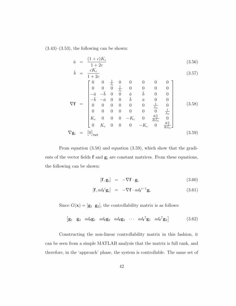
(3.43)–(3.53), the following can be shown:
a =(1 + c)Kc
1 + 2c(3.56)
b =cKc
1 + 2c(3.57)
∇f =
0 0 1J1
0 0 0 0 0
0 0 0 1J1
0 0 0 0
−a −b 0 0 a b 0 0−b −a 0 0 b a 0 00 0 0 0 0 0 1
Jm0
0 0 0 0 0 0 0 1Jm
Kc 0 0 0 −Kc 0K2
T
RJm0
0 Kc 0 0 0 −Kc 0K2
T
RJm
(3.58)
∇gi =[0]
8x8(3.59)
From equation (3.58) and equation (3.59), which show that the gradi-
ents of the vector fields f and gi are constant matrices. From these equations,
the following can be shown:
[f ,gi] = −∇f · gi (3.60)
[f , adfigi] = −∇f · adf i−1gi (3.61)
Since G(x) = [g1 g2], the controllability matrix is as follows:
[g1 g2 adfg1 adfg2 adfg2 · · · adf
7g1 adf7g2
](3.62)
Constructing the non-linear controllability matrix in this fashion, it
can be seen from a simple MATLAB analysis that the matrix is full rank, and
therefore, in the ‘approach’ phase, the system is controllable. The same set of
42

equations (with minor changes) can be used to prove that the system is also
controllable in the ‘completion’ phase. In the modes with obstructed ports or
shunts, the system can be shown to be controllable using a similar method.
3.2.2 Observability
For non-linear systems, the observability can be analyzed using Lie
derivatives [6], and this method is analogous to using the rank of the observ-
ability matrix to determine observability in the case of linear systems. Given
the output of a system,
y = Ψ(x) (3.63)
Also, since x = f(x,u), the direction of the vector field f can be changed
using u(t). Now, the directional derivative, or the Lie derivative, Lfi(ψj), is
defined as
Lfi(ψj) =∂ψj∂x· fi (3.64)
where fi is the state derivative vector when the only active element of the
control input, u, is ui = 1, and the other control input elements are zero. Let
G be the set of all possible linear combinations of these smooth functions, and
∂G∂x
be the set of all their gradients. If these set of vector fields span Rn, then
the system is weakly observable.
Using this analysis, the observability conditions are examined for the
nominal model of the pump during the ‘approach’ phase. A similar method
43

may be used to determine whether the system is observable in the other modes.
In the system model, there are two outputs, i.e., the two angular positions of
the motors, θ1m and θ3m. Therefore,
y =
[θ1m
θ3m
](3.65)
y =
[Lfi(ψ1)Lfi(ψ2)
](3.66)
=
[h1mJmh3mJm
](3.67)
y =
[Lfi
2(ψ1)Lfi
2(ψ2)
](3.68)
=
1Jm
(KT
R
(E1 − KT
Jmh1m
)−Kc(θ1m − θ1)
)1Jm
(KT
R
(E3 − KT
Jmh3m
)−Kc(θ3m − θ3)
) (3.69)
...y =
[Lfi
3(ψ1)Lfi
3(ψ2)
](3.70)
=
1Jm
(KT
R
(E1 − KT
Jmh1m
)−Kc(
h1mJm− h1
J))
1Jm
(KT
R
(E3 − KT
Jmh3m
)−Kc(
h3mJm− h3
J)) (3.71)
Defining G and ∂G∂x
as before, the following can be derived:
a =K4T
R2J3m
− Kc
J2m
(3.72)
∇G =
0 0 0 0 1 0 0 00 0 0 0 0 1 0 00 0 0 0 0 0 1
Jm0
0 0 0 0 0 0 0 1Jm
Kc
Jm0 0 0 −Kc
Jm0
−K2T
RJ2m
0
0 Kc
Jm0 0 0 −Kc
Jm0
−K2T
RJ2m
−K2TKc
RJ2m
0 Kc
JmJ0
K2TKc
RJ2m
0 a 0
0−K2
TKc
RJ2m
0 Kc
JmJ0
K2TKc
RJ2m
0 a
(3.73)
44
In the calculation of ∇G, it is assumed that the the first control input
is a constant, and the other is taken as zero. Therefore, the derivatives of
these control inputs with respect to the states are always zero. Repeating the
method with the second control input activated generates the same matrix,
and therefore, is not necessary. Since ∇G is a constant matrix and is full
rank, the system is observable in the ‘approach’ phase. For the other modes,
a similar analysis shows that the nominal plant model is always observable.
Equations (3.65)–(3.71) also show that the two relative orders of the system
associated with each of the outputs, r1 and r2, are both r1 = r2 = 2.
3.3 Observer Design
When a model-based controller has to be designed, a full-state feedback
may be required. However, since the system has only two outputs, the states
are not directly available. Since the nominal plant model is observable in all
modes, as shown in Section 3.2, a modified Luenberger Observer [6] can there-
fore be designed for full-state feedback. For a non-linear system represented
as
x = f(x) +G(x)u (3.74)
y = Ψ(x) (3.75)
If the estimated state vector is x, the observer dynamics can be repre-
45
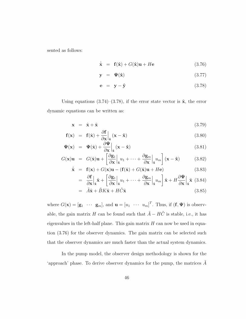
sented as follows:
˙x = f(x) +G(x)u +He (3.76)
y = Ψ(x) (3.77)
e = y − y (3.78)
Using equations (3.74)–(3.78), if the error state vector is x, the error
dynamic equations can be written as:
x = x + x (3.79)
f(x) = f(x) +∂f
∂x
∣∣∣x
(x− x) (3.80)
Ψ(x) = Ψ(x) +∂Ψ
∂x
∣∣∣x
(x− x) (3.81)
G(x)u = G(x)u +
[∂g1
∂x
∣∣∣xu1 + · · ·+ ∂gm
∂x
∣∣∣xum
](x− x) (3.82)
˙x = f(x) +G(x)u− (f(x) +G(x)u +He) (3.83)
=∂f
∂x
∣∣∣xx +
[∂g1
∂x
∣∣∣xu1 + · · ·+ ∂gm
∂x
∣∣∣xum
]x +H
∂Ψ
∂x
∣∣∣xx (3.84)
= Ax + BKx +HCx (3.85)
where G(x) = [g1 · · · gm], and u = [u1 · · · um]T . Thus, if (f ,Ψ) is observ-
able, the gain matrix H can be found such that A−HC is stable, i.e., it has
eigenvalues in the left-half plane. This gain matrix H can now be used in equa-
tion (3.76) for the observer dynamics. The gain matrix can be selected such
that the observer dynamics are much faster than the actual system dynamics.
In the pump model, the observer design methodology is shown for the
‘approach’ phase. To derive observer dynamics for the pump, the matrices A
46
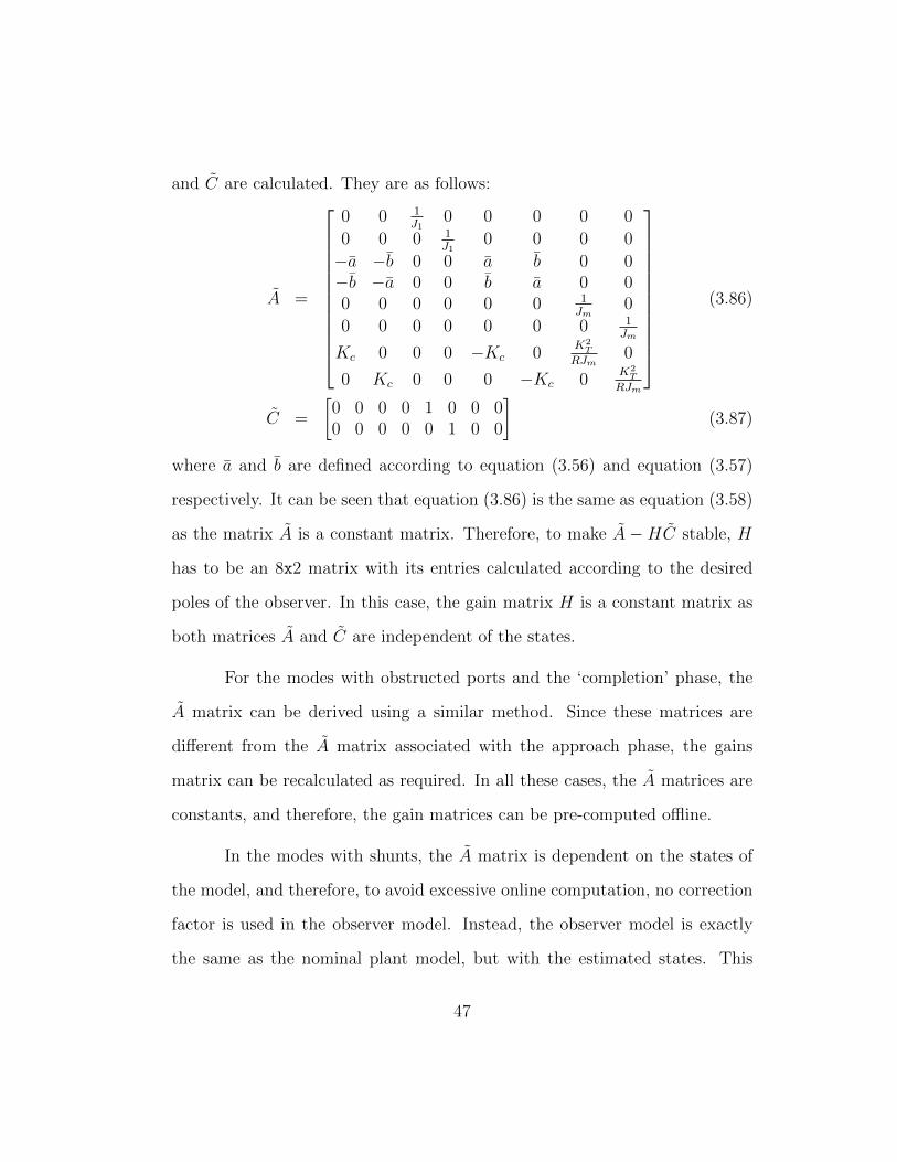
and C are calculated. They are as follows:
A =
0 0 1J1
0 0 0 0 0
0 0 0 1J1
0 0 0 0
−a −b 0 0 a b 0 0−b −a 0 0 b a 0 00 0 0 0 0 0 1
Jm0
0 0 0 0 0 0 0 1Jm
Kc 0 0 0 −Kc 0K2
T
RJm0
0 Kc 0 0 0 −Kc 0K2
T
RJm
(3.86)
C =
[0 0 0 0 1 0 0 00 0 0 0 0 1 0 0
](3.87)
where a and b are defined according to equation (3.56) and equation (3.57)
respectively. It can be seen that equation (3.86) is the same as equation (3.58)
as the matrix A is a constant matrix. Therefore, to make A −HC stable, H
has to be an 8x2 matrix with its entries calculated according to the desired
poles of the observer. In this case, the gain matrix H is a constant matrix as
both matrices A and C are independent of the states.
For the modes with obstructed ports and the ‘completion’ phase, the
A matrix can be derived using a similar method. Since these matrices are
different from the A matrix associated with the approach phase, the gains
matrix can be recalculated as required. In all these cases, the A matrices are
constants, and therefore, the gain matrices can be pre-computed offline.
In the modes with shunts, the A matrix is dependent on the states of
the model, and therefore, to avoid excessive online computation, no correction
factor is used in the observer model. Instead, the observer model is exactly
the same as the nominal plant model, but with the estimated states. This
47
can be justified in two ways. Firstly, the nominal plant models already re-
quire more computation in these modes because of the presence of algebraic
loops, and generating an extra gain matrix at each time step only adds to the
computational burden. Secondly, since these modes are to be avoided during
the transition phase, the time spent by the pistons in these modes will be
negligible.
Since the nominal model is hybrid, with the activation of the different
modes depending on the relative positions of the pistons with the ports, the
performance of the modified Luenberger observer becomes more critical to the
model. This is because the estimates of the piston positions are now used to
switch between modes in the controllers. The controllers will be described in
the following sections.
3.4 Error-Based Methods – PID Control
It has been established that the system is controllable, the first control
method used to make the two pistons track the respective desired trajectories
is the Proportional-Integral-Derivative (PID) controller. The PID controller
is an error-based controller which has been widely studied and implemented
in control systems [5, 25], and is used as the base controller for performance
comparisons in this thesis.
Given an error e = yref −y, where y is the output signal and yref is the
48
reference signal, the PID control input to the system is given as [25]:
u(t) = KP e+KDde
dt+KI
∫ t
0
e(τ)dτ (3.88)
Therefore, the control input is just the addition of three different ac-
tions: proportional gain, the integral term and derivative feedback. The gains
in the control input, KP , KD and KI , are the proportional, derivative and
integral gains respectively.
In the pump model, the outputs of the system are the angular positions
of the motors, θ1m and θ3m, as shown in equation (3.65). However, the desired
trajectories are specified as variation of angular positions of the pistons, θ1,des
and θ2,des, with respect to time. Therefore, the assumption is made that
the estimated states of the motors are approximately equal to those of the
estimated states of the pistons because of the high coupling stiffness and the
natural stability of the pistons under small displacements. Therefore, the
following equations can be written:
e1 = θ1,des − θ1 (3.89)
≈ θ1,des − θ1,est (3.90)
≈ θ1,des − θ1m,est (3.91)
e3 = θ3,des − θ3 (3.92)
≈ θ3,des − θ3,est (3.93)
≈ θ3,des − θ3m,est (3.94)
49
Using equations (3.89)–(3.94), the expressions for the control input can
now be derived for the PID controller. They are as follows:
E1 = KP e1 +KDde1
dt+KI
∫ t
0
e1dτ (3.95)
= KP (θ1,des − θ1m,est) +KD(θ1,des − θ1m,est) (3.96)
+KI
∫ t
0
(θ1,des − θ1m,est)dτ
= KP (θ1,des − θ1m,est) +KD(ω1,des − ω1m,est) (3.97)
+KI
∫ t
0
(θ1,des − θ1m,est)dτ
E3 = KP e3 +KDde3
dt+KI
∫ t
0
e3(τ)dτ (3.98)
= KP (θ3,des − θ3m,est) +KD(θ3,des − θ3m,est) (3.99)
+KI
∫ t
0
(θ3,des − θ3m,est)dτ
= KP (θ3,des − θ3m,est) +KD(ω3,des − ω3m,est) (3.100)
+KI
∫ t
0
(θ3,des − θ3m,est)dτ
This modified PID controller uses the angular velocities of the motors
for the derivative action. Since the derivative of the desired angular positions,
i.e., the desired angular velocities, ω1,des and ω3,des are also available, they can
be directly used in the control inputs, which are the voltages provided to the
motors, E1 and E3. In the actual implementation, an appropriately filtered
version of the estimated angular velocities of the motors can be used to avoid
issues due to noise in motor encoder data.
The block diagram for the PID controller is shown in Fig. 3.4. In the
PID controller, the control input to each actuator is dependent only on the
50

error variables of that piston, i.e., each control input is independent of the
dynamics and error states of the other piston. The output from the actuators
are the torques to the pistons, τ1 and τ3. It has to be noted that in the PID
controller, the coupling between the dynamics of the two pistons is ignored,
forcing the controller to compensate for those effects as disturbances.
𝜃1,𝑑𝑒𝑠
𝜔1,𝑑𝑒𝑠
Observer
Pump
Actuator 1
Actuator 2
𝜏1
𝜏3
𝜃3,𝑑𝑒𝑠
𝜔3,𝑑𝑒𝑠
Controller 1
Controller 2
𝜃1𝑚, 𝜃3𝑚
Σ
Σ
Σ
Σ
𝐸1
𝐸3
𝜃1𝑚,𝑒𝑠𝑡
𝜔1𝑚,𝑒𝑠𝑡
𝜃3𝑚,𝑒𝑠𝑡
𝜔3𝑚,𝑒𝑠𝑡
+
+
+
+
-
-
-
-
Figure 3.4: Block diagram for PID controller.
3.5 Model-Based Methods – Cascaded Control
Model-based controllers use the dynamics of the nominal model of the
plant in order to make the system follow a desired trajectory. The controller
presented in this section uses a cascaded model-based structure, consisting of
51
a feedback-linearized part to determine the desired torque, and a sliding mode
controller to track this desired torque. This controller, therefore, incorporates
inter-piston coupling unlike the PID controller, which accounts for these effects
as unmodeled disturbances.
3.5.1 Outer Loop – Feedback-Linearized Control
To design the outer loop, equations (3.43)–(3.53) for the ‘approach’
phase can be used after slight modification:
c = ρ(V1 + V3)R2t /J (3.101)
Z1 = (Pin − Pout)A1Rt (3.102)
Z3 = −Z1 (3.103)
θ1 = h1/J (3.104)
h1 =(1 + c)Z1 + cZ3
1 + 2c+
(1 + c)τ1 + cτ3
1 + 2c(3.105)
θ3 = h3/J (3.106)
h3 =(1 + c)Z3 + cZ1
1 + 2c+
(1 + c)τ3 + cτ1
1 + 2c(3.107)
θ1m = h1m/Jm (3.108)
h1m =KT
R
(E1 −KTh1m/Jm
)−Kc(θ1m − θ1) (3.109)
θ3m = h3m/Jm (3.110)
h3m =KT
R
(E3 −KTh3m/Jm
)−Kc(θ3m − θ3) (3.111)
The equations (3.104)–(3.111) are applicable to all the nominal models
with minor changes to equation (3.102) and equation (3.103) according to the
52
case currently activated. The actuator torque outputs have been represented
by τ1 and τ3 in these equations. The errors in the system can be defined as:
e1 = θ1,des − θ1 (3.112)
≈ θ1,des − θ1,est (3.113)
e3 = θ3,des − θ3 (3.114)
≈ θ3,des − θ3,est (3.115)
For the outer loop, only the pump model (without the actuators) is
considered, i.e., equations (3.104)–(3.107). If the estimated positions of the
pistons, θ1,est and θ3,est, are considered as virtual outputs of the the pump
model without actuators, and the torques, τ1 and τ3, are considered as inputs,
the relative order for each of these virtual outputs would be 2. Therefore, a
feedback-linearized control [24] for this reduced pump model can be derived
as:
e1 + λ1e1 + λ2e1 = 0 (3.116)
e3 + λ1e3 + λ2e3 = 0 (3.117)
Using the definitions of e1 and e3, these can be rewritten as:
(θ1,des − θ1,est) + λ1(θ1,des − θ1,est) + λ2(θ1,des − θ1,est) = 0 (3.118)
(θ3,des − θ3,est) + λ1(θ3,des − θ3,est) + λ2(θ3,des − θ3,est) = 0 (3.119)
Using the model dynamic equations, equation (3.118) and equation
53
(3.119), the following can be written:
Φ1 =
(θ1,des −
(1 + c)Z1 + cZ3
J(1 + 2c)
)+ λ1(ω1,des − ω1,est) (3.120)
+λ2(θ1,des − θ1,est)
Φ3 =
(θ3,des −
(1 + c)Z3 + cZ1
J(1 + 2c)
)+ λ1(ω3,des − ω3,est) (3.121)
+λ2(θ3,des − θ3,est)
τ1,des = J [(1 + c)Φ1 − cΦ3] (3.122)
τ3,des = J [(1 + c)Φ3 − cΦ1] (3.123)
where Φ1 and Φ2 are defined by substituting equations (3.104)–(3.107) in equa-
tion (3.118) and equation (3.119). Equation (3.122) and equation (3.123) are
expressions for the desired torque inputs to the pump such that the desired
trajectories, θ1,des and θ3,des, are tracked. Here, λ1 and λ3 are parameters that
determine the response of the feedback-linearized output. Once the desired
torques are determined, the inner loop of the controller can be designed.
3.5.2 Inner Loop – Sliding Mode Control
Sliding mode control is a type of robust control [7, 24] in which the
control problem is changed through introduction of notational simplifications
to be represented as a first-order system. This first-order dynamic variable is
referred to as the ‘sliding’ variable or surface, and the system is always forced
towards this surface. The behavior of the system on this surface is called the
‘sliding mode’.
A sliding mode controller design for the pump model is presented in this
54

section. The desired torques from Section 3.5.1 are used to generate desired
trajectories for the angular positions of the motors. The actuator model is
now treated as two separate reduced-order systems, one for each motor, with
the inputs as the motor voltages and the outputs as the angular positions of
the motors. Therefore, the errors are defined as:
e1m = θ1m,des − θ1m (3.124)
≈ θ1m,des − θ1m,est (3.125)
e3m = θ3m,des − θ3m (3.126)
≈ θ3m,des − θ3m,est (3.127)
Examining this reduced-order actuator system, it can be seen that the
relative order for each actuator is two. Therefore, to design the first-order
sliding surface, the following equations are used:
s1 = e1m + λ3e1m (3.128)
s3 = e3m + λ3e3m (3.129)
Using the surfaces defined in equations (3.128)–(3.129), the equations
defining the sliding mode controller are as follows:
s1 = −α · sgn(s1) (3.130)
s3 = −α · sgn(s3) (3.131)
55
e1m + λ3e1m = −α · sgn(s1) (3.132)
e3m + λ3e3m = −α · sgn(s3) (3.133)
(θ1m,des − θ1m,est) = −λ3(θ1m,des − θ1m,est)− α · sgn(
(θ1m,des (3.134)
−θ1m,est) + λ3(θ1m,des − θ1m,est))
(θ3m,des − θ3m,est) = −λ3(θ3m,des − θ3m,est)− α · sgn(
(θ3m,des (3.135)
−θ3m,est)+;λ3(θ3m,des − θ3m,est))
The parameters λ3 and α can be tuned for more robustness in control
[24]. Using the constitutive relation of the magnetic coupling in the actuators,
it is known that:
τ1,des = Kc(θ1m,des − θ1,est) (3.136)
τ3,des = Kc(θ3m,des − θ3,est) (3.137)
From equation (3.136) and equation (3.137), the desired angular po-
sitions of the motors can be derived. These expressions are substituted in
equations (3.134)–(3.135) as follows:(τ1,des
Kc
+ θ1,est − θ1m,est
)= −λ3
(τ1,des
Kc
+ θ1,est − θ1m,est
)(3.138)
−α · sgn((
τ1,des
Kc
+ θ1,est − θ1m,est
)+λ3
(τ1,des
Kc
+ θ1,est − θ1m,est
))
56
(τ3,des
Kc
+ θ3,est − θ3m,est
)= −λ3
(τ3,des
Kc
+ θ3,est − θ3m,est
)(3.139)
−α · sgn((
τ3,des
Kc
+ θ3,est − θ3m,est
)+λ3
(τ3,des
Kc
+ θ3,est − θ3m,est
))The terms in equation (3.138) and equation (3.139) can be substituted
to derive the control efforts required for this cascaded control strategy. For
simplicity and in order to avoid algebraic loops, the ideal torques, τdes, are
used in the expansion of the terms τdes, θest = ωest, θm,est = ωm,est and τdes.
The control efforts, E1 and E3, are as follows:
ω1,est =(1 + c)(τ1,des + Z1) + c(τ3,des + Z3)
J(1 + 2c)(3.140)
ω3,est =(1 + c)(τ3,des + Z3) + c(τ1,des + Z1)
J(1 + 2c)(3.141)
E1 =RJmKT
(τ1,des
Kc
+ ω1,est +
(K2
Tω1m,est
R+ τ1,des
)Jm
(3.142)
+λ3
(τ1,des
Kc
+ ω1,est − ω1m,est
)+α · sgn
(τ1,des
Kc
+ ω1,est − ω1m,est + λ3
(τ1,des
Kc
+ θ1,est − θ1m,est
)))
E3 =RJmKT
(τ3,des
Kc
+ ω3,est +
(K2
Tω3m,est
R+ τ3,des
)Jm
(3.143)
+λ3
(τ3,des
Kc
+ ω3,est − ω3m,est
)+α · sgn
(τ3,des
Kc
+ ω3,est − ω3m,est + λ3
(τ3,des
Kc
+ θ3,est − θ3m,est
)))It is important to note that this cascaded control strategy uses the
57
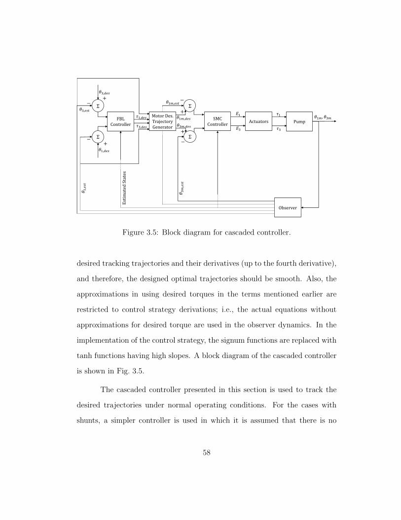
Pump𝜃1𝑚, 𝜃3𝑚
Σ
Σ
Estim
ated
States
𝜃1,𝑒𝑠𝑡
𝜃3,𝑑𝑒𝑠
𝜃1,𝑑𝑒𝑠
𝜃3,𝑒𝑠𝑡
+
+
−
−
𝜏1
𝜏3
Actuators
𝐸1
𝐸3
Σ
Σ
𝜏1,𝑑𝑒𝑠
𝜏3,𝑑𝑒𝑠
FBL Controller
𝜃1𝑚,𝑑𝑒𝑠
𝜃3𝑚,𝑑𝑒𝑠
+
+
Motor Des. Trajectory Generator
𝜃1𝑚,𝑒𝑠𝑡
𝜃3𝑚,𝑒𝑠𝑡
−
−
Observer
SMC Controller
Figure 3.5: Block diagram for cascaded controller.
desired tracking trajectories and their derivatives (up to the fourth derivative),
and therefore, the designed optimal trajectories should be smooth. Also, the
approximations in using desired torques in the terms mentioned earlier are
restricted to control strategy derivations; i.e., the actual equations without
approximations for desired torque are used in the observer dynamics. In the
implementation of the control strategy, the signum functions are replaced with
tanh functions having high slopes. A block diagram of the cascaded controller
is shown in Fig. 3.5.
The cascaded controller presented in this section is used to track the
desired trajectories under normal operating conditions. For the cases with
shunts, a simpler controller is used in which it is assumed that there is no
58
magnetic coupling in the actuators; i.e., the coupling is infinitely rigid. There-
fore, once the desired torques are derived using the feedback-linearized outer
loop, the voltages to be supplied to the actuators can be directly calculated.
A simpler control strategy is used for these modes for the same reasons as
presented in Section 3.3. Alternatively, a PID control strategy can also be
used for tracking in these modes to reduce computational load.
3.6 Summary
This chapter presented two control strategies for desired trajectory
tracking – the PID controller, which is error-based and treats the coupling be-
tween the pistons as unmodeled dynamics, and the cascaded controller, which
is based on the nominal plant model presented in this chapter and accounts for
the coupling in piston dynamics. The controllability and observability of the
nominal plant model were also verified, and an Extended Luenberger Observer
was designed for full-state feedback.
These two control strategies will be tested on the complete pump model
in Chapter 4 for performance and robustness characterization.
59
Chapter 4
Simulation Results
The comparison between the control strategies that have been pre-
sented in Chapter 3 are presented in this chapter. The control strategies are
implemented on the TORVADTM pump model with parameters defined in Ap-
pendix A. The results are presented in two parts: first, the performances of
these control strategies are compared under ideal operating conditions, and
second, the robustness of each controller is tested.
4.1 Performance Comparison of Control Strategies
The performances of the control strategies are evaluated under ideal
operating conditions with constant inlet/outlet pressures. A set of testing
trajectories are defined as follows:
θ1,des(t) =A
2sin
(πt
2T
)(4.1)
θ3,des(t) = A− A
2cos
(πt
2T
)(4.2)
where T is the time period for the transition phase, and A is the angular width
of the transition phase. These testing trajectories have been designed to force
the system into the shunt mode to enable performance of the control strategies
for these modes to also be evaluated. In the normal operation of the pump, the
60
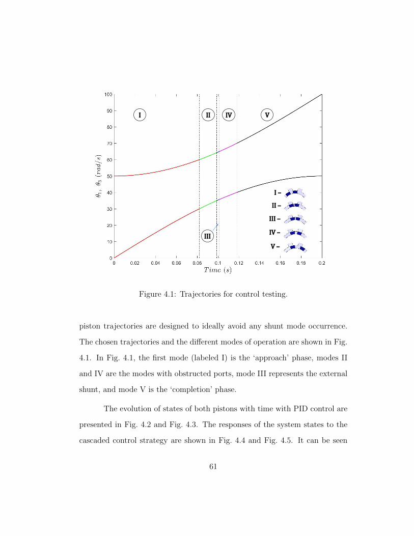
I II IV V
I –
II –
III –
IV –
V –
III
Figure 4.1: Trajectories for control testing.
piston trajectories are designed to ideally avoid any shunt mode occurrence.
The chosen trajectories and the different modes of operation are shown in Fig.
4.1. In Fig. 4.1, the first mode (labeled I) is the ‘approach’ phase, modes II
and IV are the modes with obstructed ports, mode III represents the external
shunt, and mode V is the ‘completion’ phase.
The evolution of states of both pistons with time with PID control are
presented in Fig. 4.2 and Fig. 4.3. The responses of the system states to the
cascaded control strategy are shown in Fig. 4.4 and Fig. 4.5. It can be seen
61
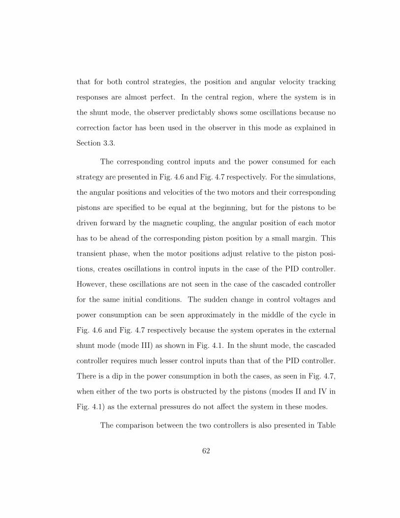
that for both control strategies, the position and angular velocity tracking
responses are almost perfect. In the central region, where the system is in
the shunt mode, the observer predictably shows some oscillations because no
correction factor has been used in the observer in this mode as explained in
Section 3.3.
The corresponding control inputs and the power consumed for each
strategy are presented in Fig. 4.6 and Fig. 4.7 respectively. For the simulations,
the angular positions and velocities of the two motors and their corresponding
pistons are specified to be equal at the beginning, but for the pistons to be
driven forward by the magnetic coupling, the angular position of each motor
has to be ahead of the corresponding piston position by a small margin. This
transient phase, when the motor positions adjust relative to the piston posi-
tions, creates oscillations in control inputs in the case of the PID controller.
However, these oscillations are not seen in the case of the cascaded controller
for the same initial conditions. The sudden change in control voltages and
power consumption can be seen approximately in the middle of the cycle in
Fig. 4.6 and Fig. 4.7 respectively because the system operates in the external
shunt mode (mode III) as shown in Fig. 4.1. In the shunt mode, the cascaded
controller requires much lesser control inputs than that of the PID controller.
There is a dip in the power consumption in both the cases, as seen in Fig. 4.7,
when either of the two ports is obstructed by the pistons (modes II and IV in
Fig. 4.1) as the external pressures do not affect the system in these modes.
The comparison between the two controllers is also presented in Table
62
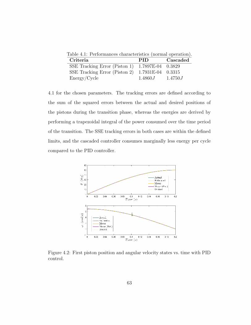
Table 4.1: Performances characteristics (normal operation).Criteria PID CascadedSSE Tracking Error (Piston 1) 1.7897E-04 0.3829SSE Tracking Error (Piston 2) 1.7931E-04 0.3315Energy/Cycle 1.4860J 1.4750J
4.1 for the chosen parameters. The tracking errors are defined according to
the sum of the squared errors between the actual and desired positions of
the pistons during the transition phase, whereas the energies are derived by
performing a trapezoidal integral of the power consumed over the time period
of the transition. The SSE tracking errors in both cases are within the defined
limits, and the cascaded controller consumes marginally less energy per cycle
compared to the PID controller.
Figure 4.2: First piston position and angular velocity states vs. time with PIDcontrol.
63
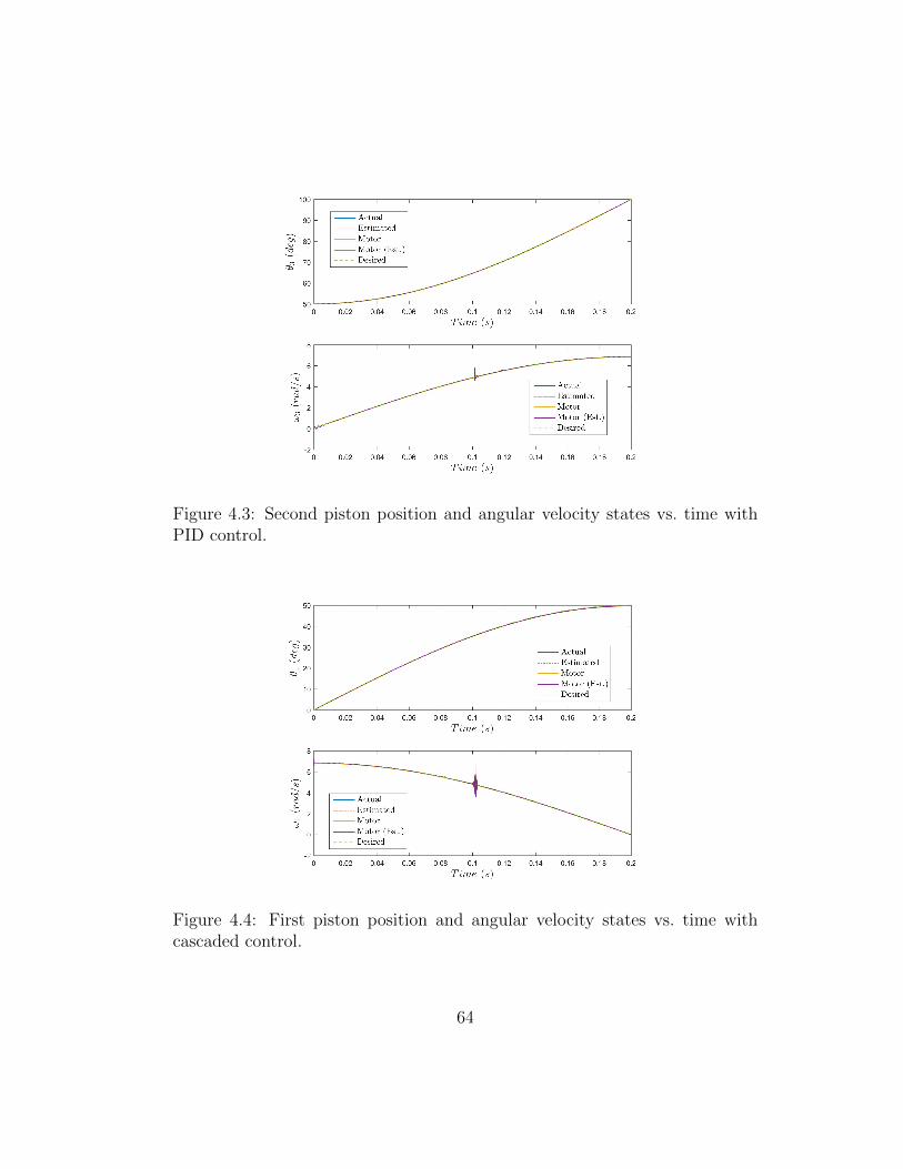
Figure 4.3: Second piston position and angular velocity states vs. time withPID control.
Figure 4.4: First piston position and angular velocity states vs. time withcascaded control.
64

Figure 4.5: Second piston position and angular velocity states vs. time withcascaded control.
Figure 4.6: Comparison of control inputs for the two control strategies.
65
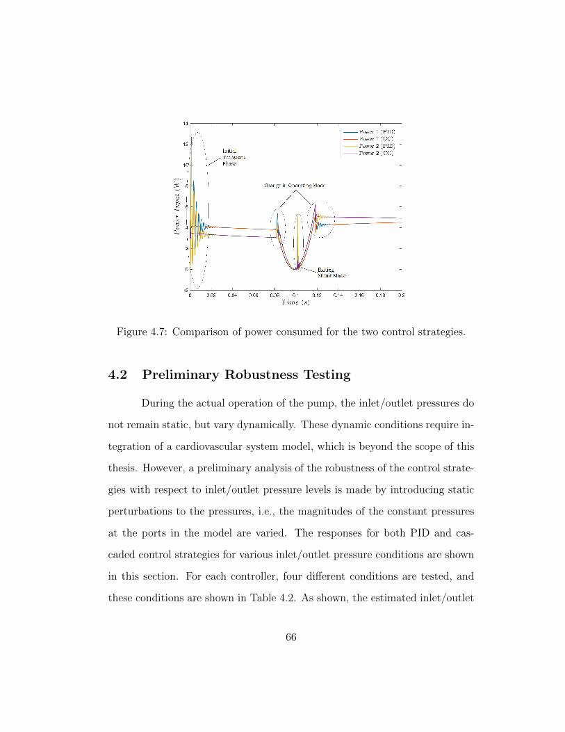
Figure 4.7: Comparison of power consumed for the two control strategies.
4.2 Preliminary Robustness Testing
During the actual operation of the pump, the inlet/outlet pressures do
not remain static, but vary dynamically. These dynamic conditions require in-
tegration of a cardiovascular system model, which is beyond the scope of this
thesis. However, a preliminary analysis of the robustness of the control strate-
gies with respect to inlet/outlet pressure levels is made by introducing static
perturbations to the pressures, i.e., the magnitudes of the constant pressures
at the ports in the model are varied. The responses for both PID and cas-
caded control strategies for various inlet/outlet pressure conditions are shown
in this section. For each controller, four different conditions are tested, and
these conditions are shown in Table 4.2. As shown, the estimated inlet/outlet
66
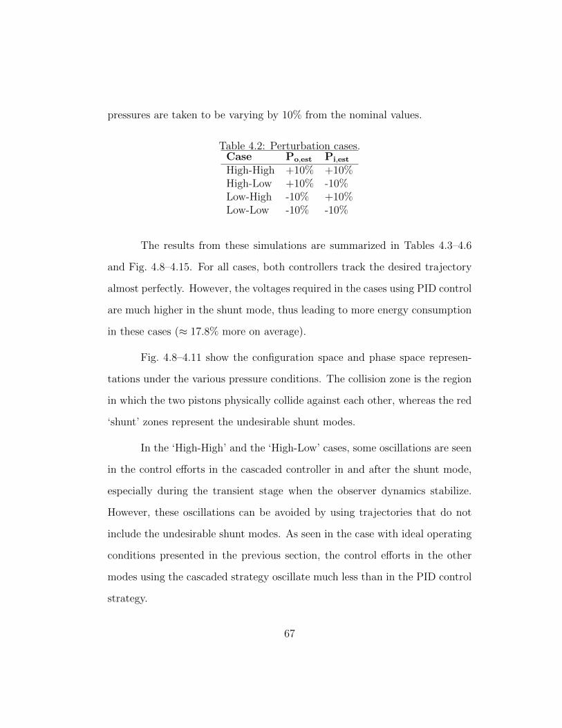
pressures are taken to be varying by 10% from the nominal values.
Table 4.2: Perturbation cases.Case Po,est Pi,est
High-High +10% +10%High-Low +10% -10%Low-High -10% +10%Low-Low -10% -10%
The results from these simulations are summarized in Tables 4.3–4.6
and Fig. 4.8–4.15. For all cases, both controllers track the desired trajectory
almost perfectly. However, the voltages required in the cases using PID control
are much higher in the shunt mode, thus leading to more energy consumption
in these cases (≈ 17.8% more on average).
Fig. 4.8–4.11 show the configuration space and phase space represen-
tations under the various pressure conditions. The collision zone is the region
in which the two pistons physically collide against each other, whereas the red
‘shunt’ zones represent the undesirable shunt modes.
In the ‘High-High’ and the ‘High-Low’ cases, some oscillations are seen
in the control efforts in the cascaded controller in and after the shunt mode,
especially during the transient stage when the observer dynamics stabilize.
However, these oscillations can be avoided by using trajectories that do not
include the undesirable shunt modes. As seen in the case with ideal operating
conditions presented in the previous section, the control efforts in the other
modes using the cascaded strategy oscillate much less than in the PID control
strategy.
67
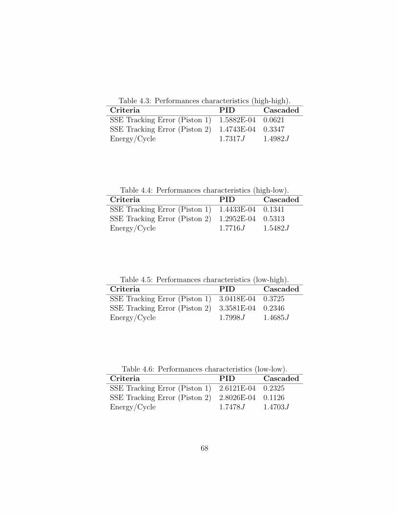
Table 4.3: Performances characteristics (high-high).Criteria PID CascadedSSE Tracking Error (Piston 1) 1.5882E-04 0.0621SSE Tracking Error (Piston 2) 1.4743E-04 0.3347Energy/Cycle 1.7317J 1.4982J
Table 4.4: Performances characteristics (high-low).Criteria PID CascadedSSE Tracking Error (Piston 1) 1.4433E-04 0.1341SSE Tracking Error (Piston 2) 1.2952E-04 0.5313Energy/Cycle 1.7716J 1.5482J
Table 4.5: Performances characteristics (low-high).Criteria PID CascadedSSE Tracking Error (Piston 1) 3.0418E-04 0.3725SSE Tracking Error (Piston 2) 3.3581E-04 0.2346Energy/Cycle 1.7998J 1.4685J
Table 4.6: Performances characteristics (low-low).Criteria PID CascadedSSE Tracking Error (Piston 1) 2.6121E-04 0.2325SSE Tracking Error (Piston 2) 2.8026E-04 0.1126Energy/Cycle 1.7478J 1.4703J
68
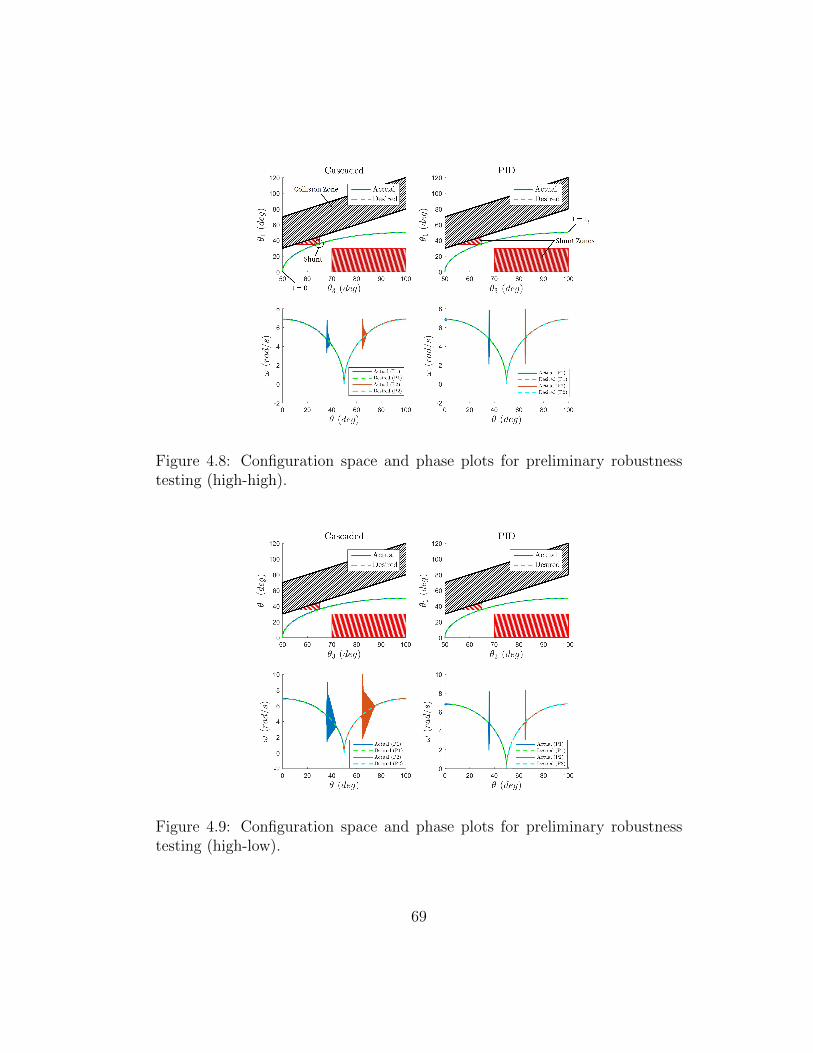
Figure 4.8: Configuration space and phase plots for preliminary robustnesstesting (high-high).
Figure 4.9: Configuration space and phase plots for preliminary robustnesstesting (high-low).
69
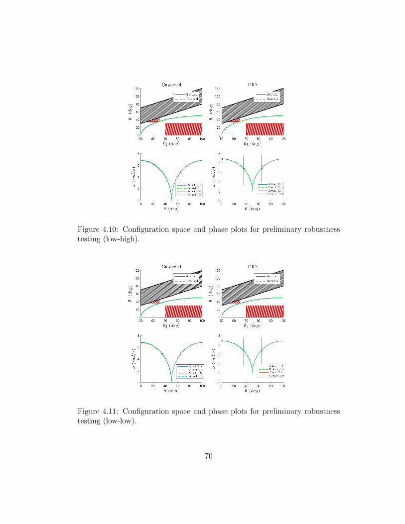
Figure 4.10: Configuration space and phase plots for preliminary robustnesstesting (low-high).
Figure 4.11: Configuration space and phase plots for preliminary robustnesstesting (low-low).
70

Figure 4.12: Comparison of control inputs for the two control strategies (high-high).
Figure 4.13: Comparison of control inputs for the two control strategies (high-low).
71
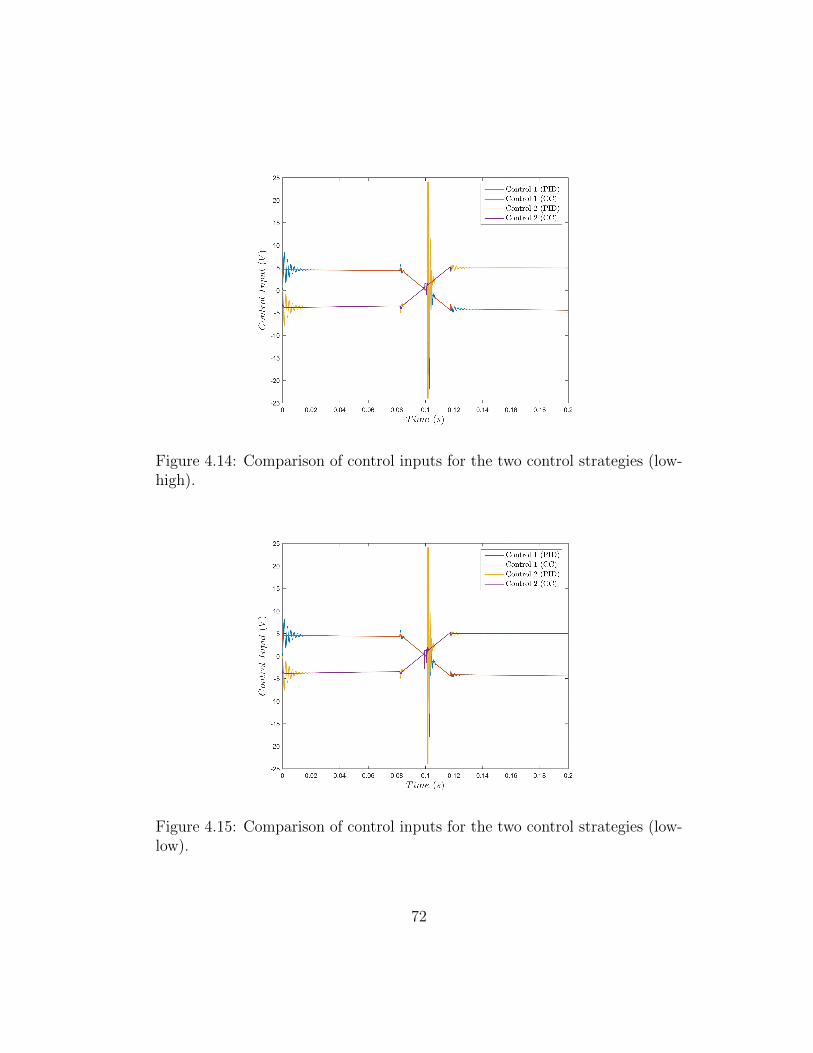
Figure 4.14: Comparison of control inputs for the two control strategies (low-high).
Figure 4.15: Comparison of control inputs for the two control strategies (low-low).
72
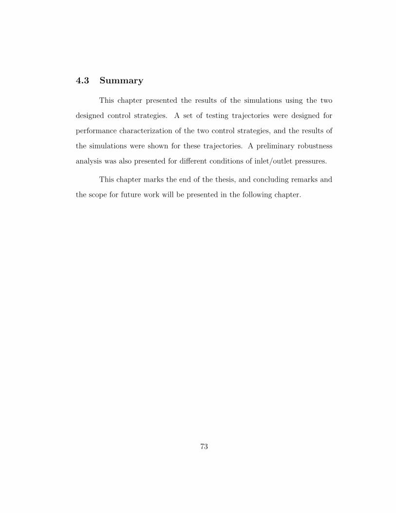
4.3 Summary
This chapter presented the results of the simulations using the two
designed control strategies. A set of testing trajectories were designed for
performance characterization of the two control strategies, and the results of
the simulations were shown for these trajectories. A preliminary robustness
analysis was also presented for different conditions of inlet/outlet pressures.
This chapter marks the end of the thesis, and concluding remarks and
the scope for future work will be presented in the following chapter.
73

Chapter 5
Conclusions and Future Work
5.1 Conclusions
The goal of this thesis was to create a working multi-energetic model
for simulating the transition dynamics in the two-piston toroidal blood pump
developed by WCS, called the TORVADTM, and to test different control strate-
gies for desired trajectory tracking in order to try to minimize oscillations in
control effort by accounting for coupling effects.
The first part of the thesis presented a model of the pump, which
accounts for the lumped energy storage properties of the variable-volume fluid
elements using a bond graph structure based on a formulation first presented
by Beaman and Breedveld [2]. The model also includes various resistive efforts;
e.g., the valving effects and the fluid shear. A momentum transfer model was
introduced to account for forces acting on the pistons in the pump due to the
changing direction of the fluid flow at the inlet and the outlet ports. Finally, an
actuator model was also added to the complete pump model, and the magnetic
coupling between the motor rotors and the pistons was modeled as a linear
spring. To account for different operating conditions of the pump, a hybrid
model design is used, with different modes activated according to the relative
positions of the two pistons with the inlet and the exit ports. An alternative
74
approach, not investigated here, would be to used coupled and non-linear
valves that would enable a single comprehensive model, as shown by Karnopp
[12].
The second part of the thesis presented a methodology for control de-
sign to track a desired trajectory. A simplified nominal plant model was pre-
sented that captures the essential components of the dynamics of the pistons
during the transition phase. This simplified model was developed specifically
for control design in the real system in which all the algebraic loops present
in the pump model were eliminated. Once the simplified plant model was
tested for controllability and observability, an observer was designed to esti-
mate the states of the system using an extended Luenberger method. This is
essential because the TORVADTM does not directly measure piston motion.
Using model-based techniques, a cascaded controller, consisting of a feedback-
linearized part to determine the desired torque and a sliding mode controller
to track this desired torque, was designed. The designed controller was then
tested for performance and robustness against a standard PID controller, and
was found to substantially reduce oscillations in the control voltages provided
to the motor when compared to the PID controller, especially when there is a
change in the operation mode of a piston.
The results for the two control strategies can now be examined using
a synchronous tracking trajectory designed by WCS [10]. To accomplish di-
astolic pulses during diastole, one of the pistons is held in the trap, while the
other is held at the primary static position. In synchronous pumping, these
75
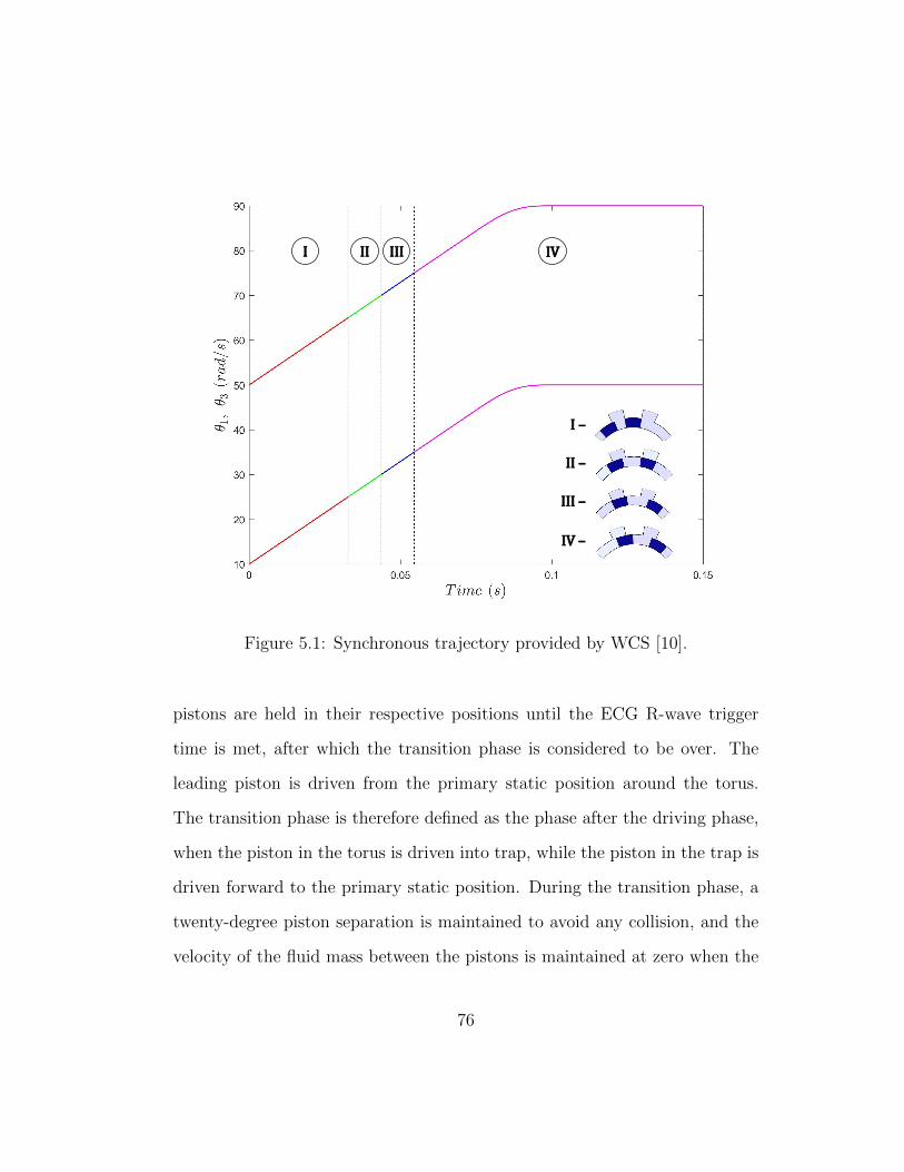
I II III IV
I –
II –
III –
IV –
Figure 5.1: Synchronous trajectory provided by WCS [10].
pistons are held in their respective positions until the ECG R-wave trigger
time is met, after which the transition phase is considered to be over. The
leading piston is driven from the primary static position around the torus.
The transition phase is therefore defined as the phase after the driving phase,
when the piston in the torus is driven into trap, while the piston in the trap is
driven forward to the primary static position. During the transition phase, a
twenty-degree piston separation is maintained to avoid any collision, and the
velocity of the fluid mass between the pistons is maintained at zero when the
76
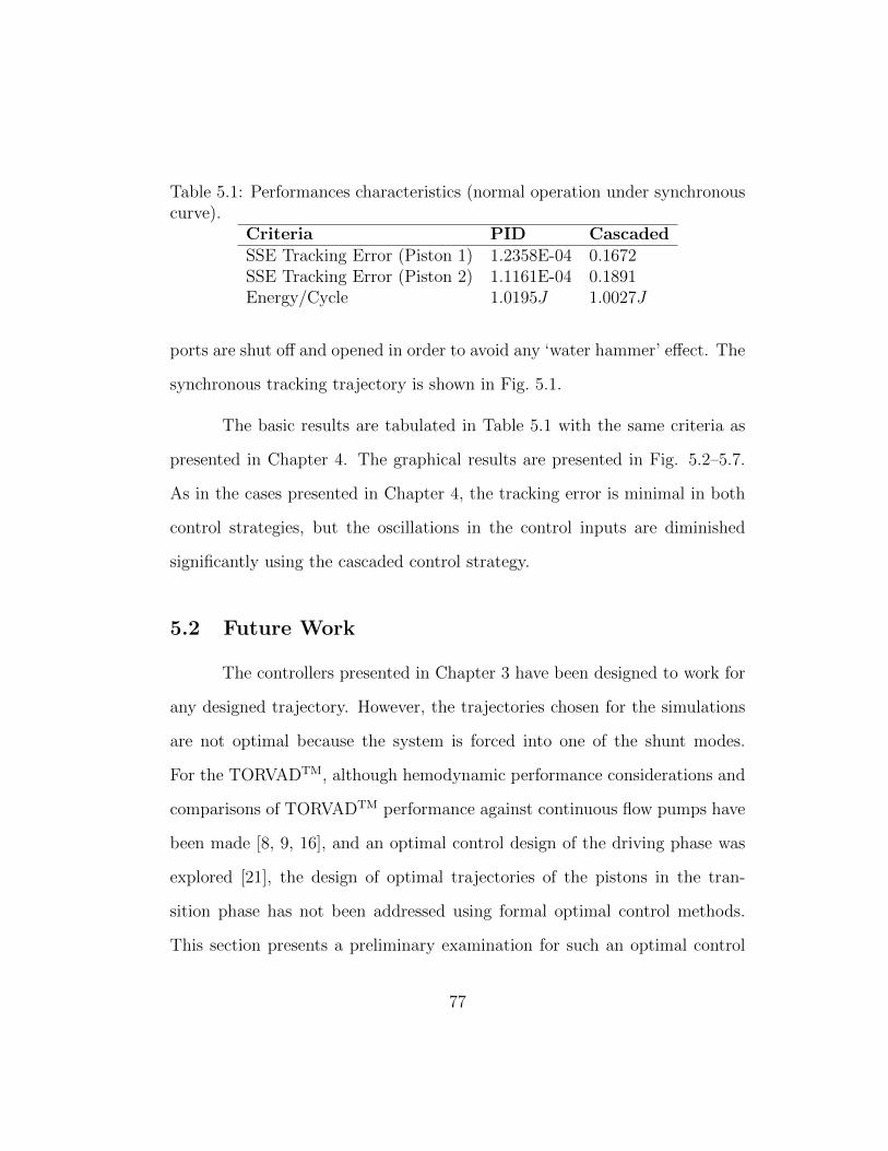
Table 5.1: Performances characteristics (normal operation under synchronouscurve).
Criteria PID CascadedSSE Tracking Error (Piston 1) 1.2358E-04 0.1672SSE Tracking Error (Piston 2) 1.1161E-04 0.1891Energy/Cycle 1.0195J 1.0027J
ports are shut off and opened in order to avoid any ‘water hammer’ effect. The
synchronous tracking trajectory is shown in Fig. 5.1.
The basic results are tabulated in Table 5.1 with the same criteria as
presented in Chapter 4. The graphical results are presented in Fig. 5.2–5.7.
As in the cases presented in Chapter 4, the tracking error is minimal in both
control strategies, but the oscillations in the control inputs are diminished
significantly using the cascaded control strategy.
5.2 Future Work
The controllers presented in Chapter 3 have been designed to work for
any designed trajectory. However, the trajectories chosen for the simulations
are not optimal because the system is forced into one of the shunt modes.
For the TORVADTM, although hemodynamic performance considerations and
comparisons of TORVADTM performance against continuous flow pumps have
been made [8, 9, 16], and an optimal control design of the driving phase was
explored [21], the design of optimal trajectories of the pistons in the tran-
sition phase has not been addressed using formal optimal control methods.
This section presents a preliminary examination for such an optimal control
77
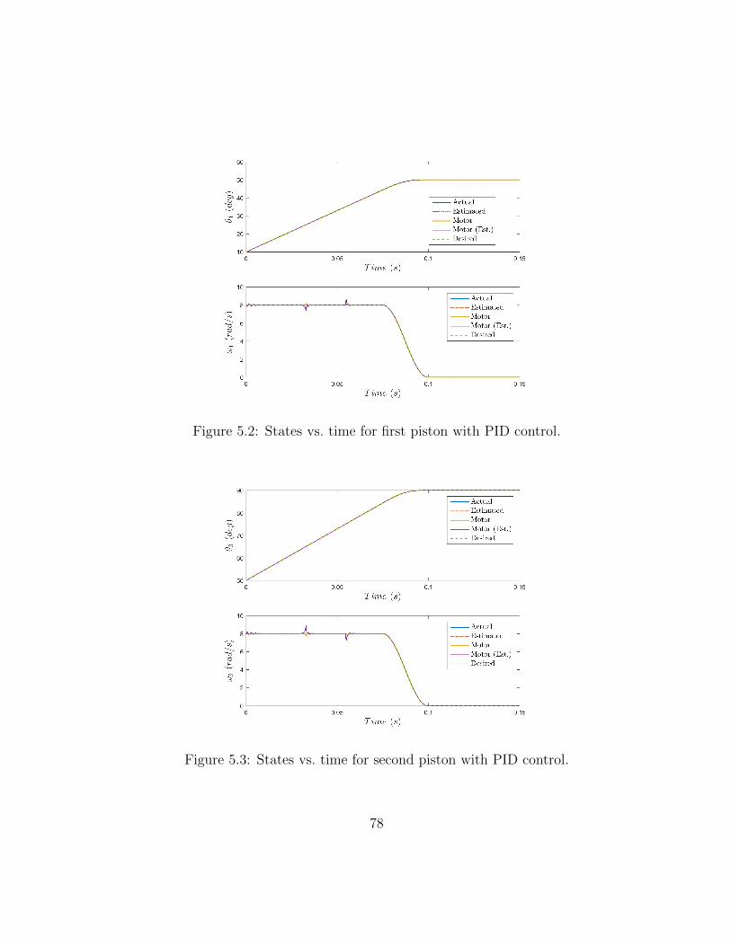
Figure 5.2: States vs. time for first piston with PID control.
Figure 5.3: States vs. time for second piston with PID control.
78

Figure 5.4: States vs. time for first piston with cascaded control.
Figure 5.5: States vs. time for second piston with cascaded control.
79
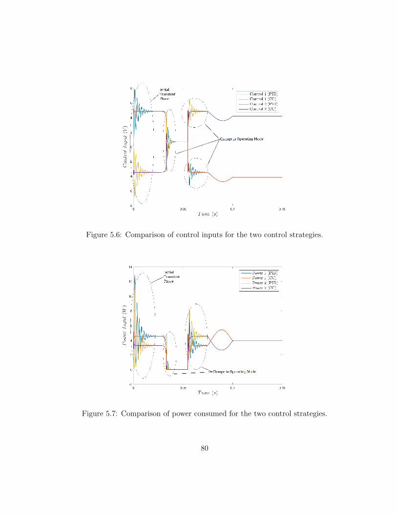
Figure 5.6: Comparison of control inputs for the two control strategies.
Figure 5.7: Comparison of power consumed for the two control strategies.
80

formulation. One objective of the optimal control approach is to find a path
for transition that requires the least energy so that battery power could be
conserved. It is also desired that the pump never operates in the shunt modes
during the transition phase, and that the pistons are only driven in the forward
direction. An approach is proposed here using the configuration space method
first presented by Lozano-Perez in his seminal paper on spatial planning [20].
Given the constraints for operation, the configuration space for the two
piston centers is shown in Fig. 5.8. In this space, the regions marked in red
are the bypass zones, and therefore, are considered to be out of bounds. The
green regions are the ‘approach’ (bottom left) and the ‘completion’ (top right)
phases, when one of the pistons is in the trap while the other travels along
the torus. The blue regions represent the modes where one or both of the two
ports, the inlet and the outlet, are covered by the pistons. The acceptable
regions are separated into different zones because of the hybrid model design,
which means that the system has different sets of equations describing the
dynamics in the different regions. The label on the X and Y-axes are the
angular positions at which the modes of operation change, and are dependent
on the positions of the inlet and the outlet ports. C and E are the center and
end positions of the transition phase respectively.
One approach to optimal control design and path planning is to de-
sign separate consequent trajectories in the ‘approach’, ‘transition’ and ‘com-
pletion’ phases separately, with matched boundary conditions. For example,
first, the optimal control path for the ‘approach’ phase is separately designed,
81
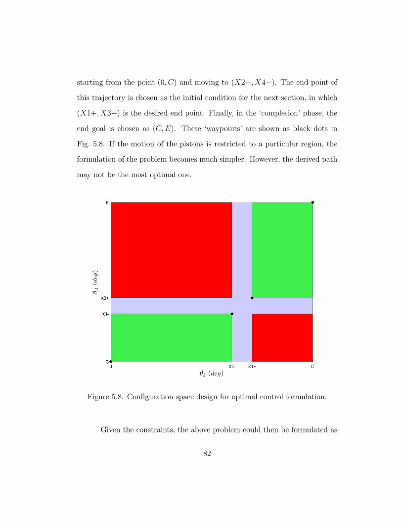
starting from the point (0, C) and moving to (X2−, X4−). The end point of
this trajectory is chosen as the initial condition for the next section, in which
(X1+, X3+) is the desired end point. Finally, in the ‘completion’ phase, the
end goal is chosen as (C,E). These ‘waypoints’ are shown as black dots in
Fig. 5.8. If the motion of the pistons is restricted to a particular region, the
formulation of the problem becomes much simpler. However, the derived path
may not be the most optimal one.
Figure 5.8: Configuration space design for optimal control formulation.
Given the constraints, the above problem could then be formulated as
82
an optimal control problem as follows:
J =
∫ tf
t0
(i1E1 + i3E3 + UTQU + S1(r1 − θ1)2 + S2(r3 − θ3)2
)dt (5.1)
+M1(r1f − θ1f )2 +M2(r3f − θ3f )
2
subject to the constraints imposed by the model dynamics as well as those
discussed earlier. In equation 5.1, E1 and E3 are the control inputs (voltages),
i1 and i3 are the corresponding currents, U is the control input vector, r1
and r3 are the reference trajectories, θ1 and θ3 are the current pistons center
positions, r1f , r3f , θ1f and θ3f are the corresponding values at time tf , Q is
a positive definite matrix, and S1, S2, M1 and M2 are positive constants. It
is to be noted that this is only a preliminary discussion, and therefore, the
discussion on the constraints is not exhaustive, e.g., constraints relating to the
‘water-hammer’ effect or the collision of pistons as presented in the design of
the synchronous trajectory design. It is also desirable to optimize relative to
the human cardiovascular hemodynamics.
If this optimal control problem is solved, paths for least energy con-
sumption can be generated, and these trajectories can then be used in the
control structure.
5.3 Summary
This thesis presented the design of a model-based control strategy for
trajectory tracking in the transition phase of the TORVADTM in order to
minimize oscillations in control voltage. A bond graph-based hybrid model
83
of the pump was designed for better understanding of the fluid-mechanical
coupling in the TORVADTM, as well as for performance comparison of the
designed controllers. Using a simplified version of the pump model as the
nominal plant, a model-based cascaded controller was designed and compared
with an error-based PID control strategy. Results for specified testing trajec-
tories, and a preliminary robustness analysis of the two control strategies were
presented, and the cascaded control strategy was shown to generate control
voltages which are much less oscillatory than that of the PID control strat-
egy. Finally, a preliminary examination of optimal path planning strategies for
transition trajectories was made in order to motivate application of formalized
optimal path planning methods in the TORVADTM.
84

Appendices
85
Appendix A
Parameters of the TORVADTM
The parameters used for simulations in Chapters 4 and 5 are derived
from parameters provided by WCS for the TORVADTM. These parameters
are listed below.
A.1 Pump Parameters
The parameters for the pump which have been used for simulation are
as follows:
Table A.1: Pump Parameters.Parameter Value Parameter ValueTorus Channel Height 1.015 in Torus Outer Radius 1.635 inTorus Inner Radius 1.335 in Mean Radius 1.485 inMean Torus Circ. 9.331 in Piston Swept Angle 200
Piston Circ. Length 0.518 in Outlet Swept Angle 150
Density, Blood 1060 kg/m3 Trap Swept Angle 200
Viscosity, Blood 1.5 mPa.s Pressure, Inlet 20 mmHgPiston Gap 0.004 in Pressure, Outlet 100 mmHgPiston Mass 0.0203 kg Piston Inertia 2.918x10⁻⁵ kg.m2
86
A.2 Motor Parameters
The two motors are modeled as permanent magnet DC motors as de-
scribed in Chapter 2. The rotor inertia of the motors is taken to be 4.18x10⁻⁶
kg.m2. The internal resistance of the motors is 4.4Ω. The torque and back-
EMF constants for the motors, KT and KV respectively, are taken to be equal
in magnitude, i.e., KT = 0.0826 N.m/A and KV = 0.0826 V.s/rad. The mag-
netic coupling is set to be 10000 N.m/rad as an approximate value, and can
be adjusted as required.
87
Bibliography
[1] DC motor speed: System modeling, Control Tutorials for MATLAB and
Simulink.
[2] J. J. Beaman and P. C. Breedveld. Physical modeling with Eulerian
frames and bond graphs. Journal of Dynamic Systems, Measurement,
and Control, 110(2):182–188, 1988.
[3] A. J. Clegg, D. A. Scott, E. Loveman, J. Colquitt, J. Hutchinson, P. Royle,
and J. Bryant. The clinical and cost-effectiveness of left ventricular assist
devices for end-stage heart failure: a systematic review and economic
evaluation. Health Technology Assessment, 45(9):1–132, 2005.
[4] J. G. Cooke. Incorporating thruster dynamics in the control of an un-
derwater vehicle. Master’s thesis, Massachusetts Institute of Technology,
September 1989.
[5] L. Desborough and R. Miller. Increasing customer value of industrial
control performance monitoring - Honeywell’s experience. In Sixth In-
ternational Conference on Chemical Process Control. AIChE Symposium
Series Number 326 (Vol. 98), 2002.
[6] E. Ergueta, R. Seifried, R. Horowitz, and M. Tomizuka. Extended Lu-
enberger observer for a MIMO nonlinear nonholonomic system. In Pro-
88
ceedings of the 17th World Congress, Seoul, Korea, July 2008. The Inter-
national Federation of Automatic Control.
[7] B. R. Fernandez and J. K. Hedrick. Control of multivariable non-linear
systems by the sliding mode method. International Journal of Control,
46(3):1019–1040, 1987.
[8] J. R. Gohean, M. J. George, K. W. Chang, E. R. Larson, T. D. Pate,
M. Kurusz, R. G. Longoria, L. Kaiser, and R. W. Smalling. Preservation
of native aortic valve flow and full hemodynamic support with the TOR-
VAD using a computational model of the cardiovascular system. ASAIO
Journal, 61(3):259–265, 2015.
[9] J. R. Gohean, M. J. George, T. D. Pate, M. Kurusz, R. G. Longoria, and
R. W. Smalling. Verification of a computational cardiovascular system
model comparing the hemodynamics of a continuous flow to a synchronous
valveless pulsatile flow left ventricular assist device. ASAIO Journal,
59(2):107–116, 2013.
[10] J.R. Gohean. TORVADTM tracking curves. Technical report, Windmill
Cardiovascular Systems, Inc., February 2008.
[11] D. Karnopp. Bond graph models for fluid dynamics systems. Journal of
Dynamic Systems, Measurement, and Control, 94(3):222–229, 1972.
[12] D. Karnopp. General method for including rapidly switching devices
in dynamic simulation system models. Trans. Society for Computer
89
Simulation, 2(1):155–168, 1985.
[13] D. Karnopp, D. Margolis, and R. Rosenberg. System Dynamics: Mod-
eling, Simulation, and Control of Mechatronic Systems. Wiley, fifth edi-
tion, 2012.
[14] D. Karnopp and R. Rosenberg. System Dynamics: A Unified Approach.
Wiley, 1975.
[15] J. Kirklin, D. C. Naftel, F. D. Pagani, R. L. Kormos, L. W. Stevenson,
E. D. Blume, M. A. Miller, J. T. Baldwin, and J. B. Young. Sixth
INTERMACS annual report: A 10,000-patient database. The Journal of
Heart and Lung Transplantation, 33(6):555–564, 2014.
[16] G. V. Letsou, T. D. Pate, J. R. Gohean, M. Kurusz, R. G. Longoria,
L. Kaiser, and R. W. Smalling. Improved left ventricular unloading
and circulatory support with synchronized pulsatile left ventricular as-
sistance compared with continuous-flow left ventricular assistance in an
acute porcine left ventricular failure model. The Journal of Thoracic and
Cardiovascular Surgery, 140(5):1181–1188, 2010.
[17] N. D. Manring and S. Zhang. Pressure transient flow forces for hydraulic
spool valves. Journal of Dynamic Systems, Measurement, and Control,
134(3):034501, 2012.
[18] D. L. Margolis. Modeling of two-stroke internal combustion engine dy-
namics using the bond graph technique. SAE Technical Paper, 750860,
90
1975.
[19] D. L. Margolis. Bond graph fluid line models for inclusion with dynamic
systems simulations. Journal of the Franklin Institute, 308(3):255–268,
1979.
[20] T. Lozano Perez. Spatial planning: A configuration space approach.
IEEE Transactions on Computing, C-32(2):108–120, 1983.
[21] E. S. Rapp. Brushless DC motor modeling and optimal control: A cardio-
vascular application. Master’s thesis, The University of Texas at Austin,
August 2016.
[22] R. C. Redfield. Bond graphs of open systems: A water rocket example.
Proceedings of the Institution of Mechanical Engineers, Part I: Journal of
Systems and Control Engineering, 220(7):607–615, 2006.
[23] R. Shoureshi and K. McLaughlin. Application of bond graphs to ther-
mofluid processes and systems. Journal of Dynamic Systems, Measure-
ment, and Control, 107(4):241–245, 1985.
[24] J. J. Slotine and W. Li. Applied Nonlinear Control. Prentice Hall, 1991.
[25] Karl J. Astrom and Richard M. Murray. Feedback Systems: An Intro-
duction for Scientists and Engineers. Princeton University Press, 2008.
[26] J. Wappenschmidt, R. Autschbach, T. Schmitz-Rode U. Steinseifer, R. Mar-
greiter, G. Klima, and A. Goetzenich. Rotary piston blood pumps: Past
91

developments and future potential of a unique pump type. Expert Review
of Medical Devices, 13(8):759–771, 2016.
[27] Frank M. White. Fluid Mechanics. McGraw-Hill, seventh edition, 2011.
92


