183
Copyright c by Ravishankar Ajjanagadde Shivarama 2002

Copyright c©
by
Ravishankar Ajjanagadde Shivarama
2002
The dissertation committee for Ravishankar Ajjanagadde Shivarama
Certifies that this is the approved version of the following dissertation:
Hamilton’s equations with Euler parameters for hybrid
particle-finite element simulation
of hypervelocity impact
Committee:
Eric P. Fahrenthold, Supervisor
Anthony Bedford
Richard H. Crawford
Raul G. Longoria
Alfred E. Traver

Hamilton’s equations with Euler parameters for hybrid
particle-finite element simulation
of hypervelocity impact
by
Ravishankar Ajjanagadde Shivarama, B.E, M.Sc (Engg)
Dissertation
Presented to the Faculty of the Graduate School of
The University of Texas at Austin
in Partial Fulfillment
of the Requirements
for the Degree of
DOCTOR OF PHILOSOPHY
The University of Texas at Austin
August 2002

UMI Number: 3108510
Copyright 2002 by
Shivarama, Ravishankar Ajanagadde
All rights reserved.
________________________________________________________
UMI Microform 3108510
Copyright 2004 ProQuest Information and Learning Company.
All rights reserved. This microform edition is protected against
unauthorized copying under Title 17, United States Code.
____________________________________________________________
ProQuest Information and Learning Company 300 North Zeeb Road
PO Box 1346 Ann Arbor, MI 48106-1346

To my parents
Acknowledgments
At the outset I would like to thank my advisor, Dr. Eric P. Fahrenthold. I
consider myself fortunate to work with him. He has been very encouraging through-
out this work. Thank you. I would like to thank Dr. Raul Longoria, firstly for
serving on my committee and secondly for providing me an opportunity to be a
teaching assistant for ME 244L. I had the privilege of being a teaching assistant for
six semesters including Fall 1997, Fall 1998, Spring 1999, Fall 1999 and Spring 2000
and Spring 2002. I have truly enjoyed it. I would also like to thank Dr. Anthony
Bedford, Dr. Richard Crawford and Dr. Alfred Traver for serving as my advisory
committee members.
My parents, my brother and sister have always stood by me and its beyond
words to quantify their love and support. Thanks to the almighty God for he has
always provided me with the inner strength to overcome in what appeared to be
an insurmountable task. I would like to thank my old buddy, my name sake friend
Ravishankar Mahadevappa who has painstakingly listened to all my frustrations
and constant cribbing. I also thank my Korean friends Kwan-Woong Gwak, Young-
Hoon Han, Donghyun Kim and Young-Keun Park for providing me good company.
Thanks to Horacio and Marc Compere for all the interesting discussions and to
Cengiz Vural, the computer geek for being there to answer my silly questions. I
would also like to thank all my current and former roommates too many to list
here, for making me feel at home away from home.
Finally, I would like to thank NASA Johnson Space Center (NAG 9-1244),
National Science Foundation (CMS 9912475), the Texas Advanced Technology Pro-
v

gram (project number 003658-0709-1999) for the research support and NASA Ames
Research Center and Texas Advanced Computing Center for their computer time.
Ravishankar Ajjanagadde Shivarama
The University of Texas at Austin
August 2002
vi

Hamilton’s equations with Euler parameters for hybrid
particle-finite element simulation
of hypervelocity impact
Publication No.
Ravishankar Ajjanagadde Shivarama, Ph.D.
The University of Texas at Austin, 2002
Supervisor: Eric P. Fahrenthold
Hypervelocity impact studies (impact velocities > 1 km/sec) encompass a wide
range of applications including development of anti-terrorist defense and orbital de-
bris shield for the International Space Station (ISS). The focus of this work is on
the development of a hybrid particle-finite element method for orbital debris shield
simulations. The problem is characterized by finite strain kinematics, strong energy
domain coupling, contact-impact, shock wave propagation and history dependent
material damage effects. A novel hybrid particle finite element method based on
Hamilton’s equations is presented. The model discretizes the continuum of inter-
est simultaneously (but not redundantly) into particles and finite elements. The
particles are ellipsoidal in shape and can translate and rotate in three dimensional
space. Rotation is described using Euler parameters. Volumetric and contact impact
effects are modeled using particles, while strength is modeled using conventional La-
grangian finite elements. The model is general enough to accommodate a wide range
of material models and equations of state.
vii

Contents
Acknowledgments v
Abstract vii
List of Tables xii
List of Figures xiv
Chapter 1 Introduction 1
1.1 Introduction . . . . . . . . . . . . . . . . . . . . . . . . . . . . . . . . 1
1.2 The problem . . . . . . . . . . . . . . . . . . . . . . . . . . . . . . . 2
1.3 Solution . . . . . . . . . . . . . . . . . . . . . . . . . . . . . . . . . . 3
1.4 Sequence of events . . . . . . . . . . . . . . . . . . . . . . . . . . . . 3
1.5 Ballistic limit curves . . . . . . . . . . . . . . . . . . . . . . . . . . . 4
1.6 Literature Review . . . . . . . . . . . . . . . . . . . . . . . . . . . . 6
1.6.1 Mesh based techniques . . . . . . . . . . . . . . . . . . . . . . 6
1.6.2 Particle methods . . . . . . . . . . . . . . . . . . . . . . . . . 7
1.6.3 Element free Galerkin and other meshless methods . . . . . . 8
1.6.4 Coupled methods . . . . . . . . . . . . . . . . . . . . . . . . . 8
1.7 Motivation and scope of research . . . . . . . . . . . . . . . . . . . . 8
viii
1.8 Dissertation Organization . . . . . . . . . . . . . . . . . . . . . . . . 9
Chapter 2 Hamiltonian formulation of three dimensional rigid body
dynamics using Euler parameters 11
2.1 Introduction . . . . . . . . . . . . . . . . . . . . . . . . . . . . . . . . 11
2.2 Preliminaries . . . . . . . . . . . . . . . . . . . . . . . . . . . . . . . 12
2.3 Euler parameters . . . . . . . . . . . . . . . . . . . . . . . . . . . . . 15
2.4 Rigid body kinematics . . . . . . . . . . . . . . . . . . . . . . . . . . 18
2.5 Equations of motion . . . . . . . . . . . . . . . . . . . . . . . . . . . 20
2.5.1 Kinetic energy . . . . . . . . . . . . . . . . . . . . . . . . . . 20
2.5.2 Potential energy . . . . . . . . . . . . . . . . . . . . . . . . . 24
2.5.3 Non-conservative forces . . . . . . . . . . . . . . . . . . . . . 24
2.5.4 Hamilton’s equations . . . . . . . . . . . . . . . . . . . . . . . 25
2.6 Thermo-mechanical coupling . . . . . . . . . . . . . . . . . . . . . . 28
2.6.1 Hamilton’s equations . . . . . . . . . . . . . . . . . . . . . . . 29
2.7 Numerical examples . . . . . . . . . . . . . . . . . . . . . . . . . . . 30
2.7.1 Single degree of freedom system . . . . . . . . . . . . . . . . . 30
2.7.2 Equations of motion . . . . . . . . . . . . . . . . . . . . . . . 31
2.7.3 Torque free motion of a rigid body . . . . . . . . . . . . . . . 35
2.7.4 Motion of a spinning top in a gravitational field . . . . . . . . 42
2.8 Conclusions . . . . . . . . . . . . . . . . . . . . . . . . . . . . . . . . 50
Chapter 3 A general hybrid particle-finite element modeling method-
ology for hypervelocity impact 51
3.1 Introduction . . . . . . . . . . . . . . . . . . . . . . . . . . . . . . . . 51
3.2 Overview of the modeling methodology . . . . . . . . . . . . . . . . . 52
3.3 Kinematics . . . . . . . . . . . . . . . . . . . . . . . . . . . . . . . . 54
ix

3.3.1 Particle kinematics . . . . . . . . . . . . . . . . . . . . . . . . 54
3.3.2 Element kinematics . . . . . . . . . . . . . . . . . . . . . . . 55
3.3.3 Density Interpolation . . . . . . . . . . . . . . . . . . . . . . 56
3.4 Kinetic Energy . . . . . . . . . . . . . . . . . . . . . . . . . . . . . . 59
3.5 Internal Energy . . . . . . . . . . . . . . . . . . . . . . . . . . . . . . 60
3.6 Conservative forces . . . . . . . . . . . . . . . . . . . . . . . . . . . . 62
3.7 Plasticity model . . . . . . . . . . . . . . . . . . . . . . . . . . . . . 63
3.7.1 Flow rule . . . . . . . . . . . . . . . . . . . . . . . . . . . . . 65
3.8 Damage evolution . . . . . . . . . . . . . . . . . . . . . . . . . . . . 66
3.9 Artificial viscosity . . . . . . . . . . . . . . . . . . . . . . . . . . . . 68
3.10 Artificial heat flux . . . . . . . . . . . . . . . . . . . . . . . . . . . . 69
3.11 Entropy as a state . . . . . . . . . . . . . . . . . . . . . . . . . . . . 69
3.12 State equations . . . . . . . . . . . . . . . . . . . . . . . . . . . . . . 71
3.13 Computational Issues . . . . . . . . . . . . . . . . . . . . . . . . . . 74
3.13.1 Integration routine . . . . . . . . . . . . . . . . . . . . . . . . 74
3.13.2 Neighbor search . . . . . . . . . . . . . . . . . . . . . . . . . 75
3.13.3 Parallel Implementation . . . . . . . . . . . . . . . . . . . . . 75
3.14 Examples . . . . . . . . . . . . . . . . . . . . . . . . . . . . . . . . . 75
3.14.1 Initial validation . . . . . . . . . . . . . . . . . . . . . . . . . 75
3.14.2 Simulation with spherical particles . . . . . . . . . . . . . . . 80
3.14.3 Simulation using ellipsoidal particles . . . . . . . . . . . . . . 106
3.15 Conclusions . . . . . . . . . . . . . . . . . . . . . . . . . . . . . . . . 123
Chapter 4 Advanced numerical simulations 124
4.1 Numerical method . . . . . . . . . . . . . . . . . . . . . . . . . . . . 125
4.2 Inhibited Shape charge(ISC) Launcher Simulations . . . . . . . . . . 127
4.2.1 Material properties . . . . . . . . . . . . . . . . . . . . . . . . 128
x
4.2.2 Whipple shield with a stand off distance 7.62 cm . . . . . . . 128
4.2.3 Whipple shield with stand off distance 11.43 cm . . . . . . . 133
4.2.4 Normal impact on dual plate aluminum shield . . . . . . . . 137
4.2.5 Multi-layer Aluminum-Nextel-Kevlar shield . . . . . . . . . . 141
4.3 Projectile shape effect . . . . . . . . . . . . . . . . . . . . . . . . . . 145
4.4 Parallel speedup . . . . . . . . . . . . . . . . . . . . . . . . . . . . . 149
4.5 Conclusion . . . . . . . . . . . . . . . . . . . . . . . . . . . . . . . . 152
Chapter 5 Summary and Future work 153
Bibliography 155
Vita 164
xi

List of Tables
2.1 Simulation parameters . . . . . . . . . . . . . . . . . . . . . . . . . . 33
2.2 Simulation parameters . . . . . . . . . . . . . . . . . . . . . . . . . . 36
2.3 Comparison between experimental and simulation results . . . . . . 39
2.4 Simulation parameters and initial conditions . . . . . . . . . . . . . . 44
2.5 Comparison between analytical and simulation results . . . . . . . . 44
3.1 Wall shock problem: simulation parameters . . . . . . . . . . . . . . 77
3.2 Depleted Uranium(DU) 0.75% Ti long rod impact on a steel plate . 81
3.3 Multi-plate shield impact, ESA benchmark case #4 . . . . . . . . . . 88
3.4 Tungsten long rod impact on a steel plate at 1.833 km/s . . . . . . . 97
3.5 Comparison between experimental and simulation results . . . . . . 97
3.6 Oblique sphere impact . . . . . . . . . . . . . . . . . . . . . . . . . . 106
3.7 DU 0.75% Ti long rod impact on a steel plate . . . . . . . . . . . . . 109
3.8 Tungsten long rod impact on a steel plate at 1.833 km/s . . . . . . . 114
3.9 Comparison between experimental and simulation results . . . . . . 114
3.10 Whipple shield impact, inhibited shaped charge projectile (SWRI test
number 7139-19) . . . . . . . . . . . . . . . . . . . . . . . . . . . . . 119
4.1 Material properties for the example simulations . . . . . . . . . . . . 128
xii

4.2 Simulation parameters for Aluminum Whipple shield, stand off 7.62
cm . . . . . . . . . . . . . . . . . . . . . . . . . . . . . . . . . . . . . 129
4.3 Simulation parameters for Aluminum Whipple shield, stand off 11.43
cm . . . . . . . . . . . . . . . . . . . . . . . . . . . . . . . . . . . . . 133
4.4 Parameters for the example simulations . . . . . . . . . . . . . . . . 137
4.5 Parameters for the example simulations . . . . . . . . . . . . . . . . 141
xiii

List of Figures
1.1 Typical orbital debris shield configuration . . . . . . . . . . . . . . . 4
1.2 Ballistic limit curves for a Whipple shield configuration, areal density
= 1.25g/cm2, 0.127cm Al 6061-T6 bumper, 10.2 cm spacing, 0.32 cm
Al 2219-T87 rear wall (labels in degrees) . . . . . . . . . . . . . . . . 5
2.1 Euler parameter representation . . . . . . . . . . . . . . . . . . . . . 16
2.2 Circular disk with a spring . . . . . . . . . . . . . . . . . . . . . . . 31
2.3 Angular momenta versus time . . . . . . . . . . . . . . . . . . . . . . 33
2.4 Total energy and percentage error in energy versus time . . . . . . . 34
2.5 Euler parameters versus time . . . . . . . . . . . . . . . . . . . . . . 34
2.6 Percentage error in euler parameter constraint time . . . . . . . . . . 35
2.7 Angular momenta versus time . . . . . . . . . . . . . . . . . . . . . . 39
2.8 Total energy versus time . . . . . . . . . . . . . . . . . . . . . . . . . 40
2.9 Percentage error in total energy versus time . . . . . . . . . . . . . . 40
2.10 Euler parameters versus time . . . . . . . . . . . . . . . . . . . . . . 41
2.11 Percentage error in euler parameter constraint versus time . . . . . . 41
2.12 Euler angles versus time . . . . . . . . . . . . . . . . . . . . . . . . . 42
2.13 Spinning top . . . . . . . . . . . . . . . . . . . . . . . . . . . . . . . 43
2.14 Energy versus time . . . . . . . . . . . . . . . . . . . . . . . . . . . . 45
xiv

2.15 Norm of the angular momenta versus time . . . . . . . . . . . . . . . 45
2.16 Spatial components of the angular momentum . . . . . . . . . . . . . 46
2.17 Center of mass location . . . . . . . . . . . . . . . . . . . . . . . . . 46
2.18 Euler parameter e0 versus time . . . . . . . . . . . . . . . . . . . . . 47
2.19 Euler parameter e1 versus time . . . . . . . . . . . . . . . . . . . . . 47
2.20 Euler parameter e2 versus time . . . . . . . . . . . . . . . . . . . . . 48
2.21 Euler parameter e3 versus time . . . . . . . . . . . . . . . . . . . . . 48
2.22 Motion of the center of mass of the top . . . . . . . . . . . . . . . . 49
3.1 Generalized forces between particles . . . . . . . . . . . . . . . . . . 62
3.2 Exact and numerical density distribution at t = 0.4µs . . . . . . . . 78
3.3 Exact and numerical velocity distribution at t = 0.4µs . . . . . . . . 78
3.4 Exact and numerical pressure distribution at t = 0.4µs . . . . . . . . 79
3.5 Exact and numerical temperature distribution at t = 0.4µs . . . . . 79
3.6 Exact and numerical entropy distribution at t = 0.4µs . . . . . . . . 80
3.7 DU 0.75% Ti long rod impact on steel plate: initial configuration,
particle plot . . . . . . . . . . . . . . . . . . . . . . . . . . . . . . . 82
3.8 DU 0.75% Ti long rod impact on steel plate: initial configuration,
element plot . . . . . . . . . . . . . . . . . . . . . . . . . . . . . . . 83
3.9 DU 0.75% Ti long rod impact on steel plate: final configuration,
particle plot . . . . . . . . . . . . . . . . . . . . . . . . . . . . . . . . 84
3.10 DU 0.75% Ti long rod impact on steel plate: final configuration,
element plot . . . . . . . . . . . . . . . . . . . . . . . . . . . . . . . 85
3.11 DU 0.75% Ti long rod impact on steel plate: projectile at the end of
the simulation . . . . . . . . . . . . . . . . . . . . . . . . . . . . . . 86
3.12 DU 0.75% Ti long rod impact on steel plate: target at the end of the
simulation . . . . . . . . . . . . . . . . . . . . . . . . . . . . . . . . . 87
xv
3.13 ESA4: initial configuration, element plot . . . . . . . . . . . . . . . . 89
3.14 ESA4: element plot at t = 67 µ secs . . . . . . . . . . . . . . . . . . 90
3.15 ESA4: element plot at t = 94 µ secs . . . . . . . . . . . . . . . . . . 91
3.16 ESA4: element plot at t = 133 µ secs . . . . . . . . . . . . . . . . . . 92
3.17 ESA4: element plot at t = 150 µ secs . . . . . . . . . . . . . . . . . . 93
3.18 ESA4: particle plot at t = 150 µ secs . . . . . . . . . . . . . . . . . . 94
3.19 ESA4: close up element plot at t = 150 µ secs . . . . . . . . . . . . . 95
3.20 ESA4: close up element plot at t = 150 µ secs . . . . . . . . . . . . . 96
3.21 Tungsten long rod on a steel plate: initial configuration, element plot 98
3.22 Tungsten long rod on a steel plate: initial configuration, particle plot 99
3.23 Tungsten long rod on a steel plate at t = 150 µ secs, element plot,
view 1 . . . . . . . . . . . . . . . . . . . . . . . . . . . . . . . . . . . 100
3.24 Tungsten long rod on a steel plate at t = 150 µ secs, element plot,
view 2 . . . . . . . . . . . . . . . . . . . . . . . . . . . . . . . . . . . 101
3.25 Tungsten long rod on a steel plate at t = 150 µ secs, particle plot . . 102
3.26 Tungsten long rod on a steel plate: target at t = 150 µ secs, element
plot . . . . . . . . . . . . . . . . . . . . . . . . . . . . . . . . . . . . 103
3.27 Tungsten long rod on a steel plate: projectile at t = 150 µ secs . . . 104
3.28 Tungsten long rod on a steel plate: target at t = 150 µ secs, color on
plastic strain . . . . . . . . . . . . . . . . . . . . . . . . . . . . . . . 105
3.29 DU 0.75% Ti long rod impact on a steel plate: Initial configuration . 107
3.30 DU 0.75% Ti long rod impact on a steel plate: Initial configuration . 108
3.31 DU 0.75% Ti long rod impact on a steel plate: Initial configuration . 111
3.32 DU 0.75% Ti long rod impact on a steel plate at t = 100µ secs . . . 112
3.33 DU 0.75% Ti long rod impact on a steel plate: wall plate at t = 100µ
secs, color on plastic strain . . . . . . . . . . . . . . . . . . . . . . . 113
xvi

3.34 Tungsten long rod on a steel plate: initial configuration, element plot 115
3.35 Tungsten long rod on a steel plate at t = 150µ secs, particle plot . . 116
3.36 Tungsten long rod on a steel plate at t = 150µ secs, element plot . . 117
3.37 Tungsten long rod on a steel plate: projectile at t = 150µ secs . . . . 118
3.38 Whipple shield impact, inhibited shaped charge projectile (SWRI test
number 7139-19) : initial configuration . . . . . . . . . . . . . . . . . 120
3.39 Whipple shield impact, inhibited shaped charge projectile (SWRI test
number 7139-19) : wall plate at t = 30.2µ secs, particle plot . . . . . 121
3.40 Whipple shield impact, inhibited shaped charge projectile (SWRI test
number 7139-19) : wall plate at t = 30.2µ secs, element plot . . . . . 122
4.1 Whipple shield impact simulation: 7.62cm stand off distance, initial
configuration, particle plot . . . . . . . . . . . . . . . . . . . . . . . . 130
4.2 Whipple shield impact simulation: 7.62cm stand off distance, particle
plot at t = 46.6 µsec with color on temperature . . . . . . . . . . . 131
4.3 Whipple shield impact simulation: 7.62cm stand off distance, element
plot at t = 46.6 µsec . . . . . . . . . . . . . . . . . . . . . . . . . . . 132
4.4 Whipple shield impact simulation: 11.43cm stand off distance, initial
configuration, particle plot . . . . . . . . . . . . . . . . . . . . . . . 134
4.5 Whipple shield impact simulation: 11.43 cm stand off distance, par-
ticle plot at 45.0 µsec with color on temperature . . . . . . . . . . . 135
4.6 Whipple shield impact simulation: 11.43 cm stand off distance, ele-
ment plot at t = 45.0 µsec . . . . . . . . . . . . . . . . . . . . . . . . 136
4.7 Aluminum dual plate shield: 8.636 cm stand off distance, initial con-
figuration, particle plot . . . . . . . . . . . . . . . . . . . . . . . . . . 138
4.8 Aluminum dual plate shield: 8.636 cm stand off distance,particle plot
at 30.7 µsec with color on temperature . . . . . . . . . . . . . . . . . 139
xvii
4.9 Aluminum dual plate shield: 8.636 cm maximum stand off distance,
element plot at 30.7 µsec . . . . . . . . . . . . . . . . . . . . . . . . 140
4.10 Aluminum Nextel Kevlar shield: 7.62 cm maximum stand off dis-
tance, initial configuration, particle plot . . . . . . . . . . . . . . . . 142
4.11 Aluminum Nextel Kevlar shield: 7.62 cm maximum stand off dis-
tance, particle plot at 46.2 µsec with color on temperature . . . . . . 143
4.12 Aluminum Nextel Kevlar shield: 7.62 cm maximum stand off dis-
tance, element plot at 46.2 µsec . . . . . . . . . . . . . . . . . . . . . 144
4.13 Wall damage for ISC projectile, Whipple shield 7.62cm stand off . . 146
4.14 Wall damage for spherical projectile, Whipple shield 7.62cm stand off 146
4.15 Wall damage for ISC projectile, Whipple shield 11.43cm stand off . 147
4.16 Wall damage for spherical projectile, Whipple shield 11.43cm stand
off . . . . . . . . . . . . . . . . . . . . . . . . . . . . . . . . . . . . . 147
4.17 Wall damage for ISC projectile, dual plate aluminum shield 8.636cm
stand off . . . . . . . . . . . . . . . . . . . . . . . . . . . . . . . . . 148
4.18 Wall damage for spherical projectile, dual plate aluminum shield
8.636cm stand off . . . . . . . . . . . . . . . . . . . . . . . . . . . . 148
4.19 Absolute speedup for a 1GB size problem on Origin2000 . . . . . . . 150
4.20 Relative speedup for a 1GB size problem on Origin2000 . . . . . . . 152
xviii

Chapter 1
Introduction
1.1 Introduction
Impact phenomena is common to many situations in engineering, like in
collision of vehicles intentionally or unintentionally, impact of a printer head against
paper as in dot matrix printers, the impact of a dropped weight on a work piece as
in forging operation, impact of a bullet against a target or impact of a meteorite on
a satellite. Although these are joined together under the broad umbrella of impact
dynamics, it is not difficult to see that the impact of a meteorite on a space craft
for example is not the same as the impact of a printer head against the paper,
the primary distinguishing factor between the two being the velocity of impact.
Materials behave differently at different velocities of impact. The effects of inertia,
wave propagation and phase transformation become increasingly important as the
impact velocity increases.
There is no general agreement on what constitutes a hypervelocity impact,
although majority of the researchers in this area would consider impact velocities in
the range of 5-15km/sec as hypervelocity impact. Studies in hypervelocity impact
1

encompass a multitude of applications including the study of meteorite impacts on
earth, development of anti-terrorist defence and orbital debris shielding of space
structures, the last one being the focus of this dissertation.
The advancement in computational science over the last several decades has
established simulation based approach as a powerful tool for analysis along with
analytical and experimental techniques. Hypervelocity impact studies have not been
immune to this development. In addition, the following factors have provided added
encouragement to look at simulation based approach as a viable tool of analysis:
• The solid materials involved in hypervelocity impact undergo elastic plastic
deformation in a multi-energy framework. Finite strain kinematics, large tem-
perature and stress gradients in the materials almost completely rule out the
use of only analytical techniques as a modeling tool.
• The limitations of existing light gas guns (LGG) to shoot projectiles at kinetic
energies in the entire range of interest has provided ample motivation for shield
design studies based on simulation.
• Simulation based approach can provide low cost and faster turn around time.
1.2 The problem
The dawn of space age has seen several countries launch space structures
into orbit. However the life of these structures are finite and once found non-
functional they are abandoned. These objects disintegrate over time into smaller
mass fragments, collectively addressed today by the term “orbital debris”. This
chunk of matter travel at extremely high velocities, posing a serious risk to orbiting
space structures such as the International Space Station (ISS) and astronauts on
2
them. The gravity of this problem has been studied in detail. The reader is referred
to [56] [38] [63] and the references there in.
1.3 Solution
F.L. Whipple [73], first mooted the idea of placing a thin sacrificial sheet
of metal ahead of the wall of an orbiting space structure. This geometrical ar-
rangement, excites the incoming debris to higher thermal energy states, causing a
partial/complete vaporization of the debris, resulting in less damage to the wall
of the space structure. A single bumper shield is also referred to as a “Whipple
shield” for obvious reasons in the literature. The concept was extended to multi-
shock shields [13] where a series of thin bumpers convert the kinetic energy of the
in-coming debris into thermal energy sufficient enough to cause melting and vapor-
ization for a large range of velocities. This results in low weight and better protection
of space structures. A typical debris shield configuration is shown in figure (1.1).
1.4 Sequence of events
An orbital debris impact can be visualized as a three phase event. In the
first phase the debris impacts onto a shield resulting in one or more of the following,
depending on the materials and other parameters involved in impact.
• Perforation of the shield
• Fragmentation of the debris
• Complete or partial vaporization of the debris
In the second phase, the solid-liquid cloud of debris expands radially before it im-
pacts the second shield or the wall plate as the case may be, which forms the third
3

d1
d2
θ
I bumper
II bumper
Projectile (Orbital debris)
Wall of thespace craft
Figure 1.1: Typical orbital debris shield configuration
phase of this whole process. The numerical simulation of this multi-energy event
requires high fidelity techniques which can handle all the three phases with ease.
1.5 Ballistic limit curves
The performance of a shield is mainly characterized by the extent of protec-
tion it offers against “damage” to the wall of the space craft. In orbital debris shield
application, the term “damage” implies perforation or a detached spall of the rear
wall. The sheer number of shield and impact parameters involved in quantifying the
ability of the shield to defeat an incoming projectile/debris has forced researchers
to take recourse to empirical techniques [11]. These empirical equations, developed
based on a number of experiments, define the ballistic limit for a shield. Figure (1.2)
4

shows ballistic limit curves for a Whipple shield, for different impact angles (in de-
grees) plotted using the ballistic limit equations developed by Eric Christiansen [11].
2 4 6 8 10 12 140
0.5
1
1.5
2
2.5
3
Impact velocity in km/s
Critica
l p
art
icle
dia
me
ter
cm
60
45
30
0
No perforation or detatched spall below the curves
Figure 1.2: Ballistic limit curves for a Whipple shield configuration, areal density= 1.25g/cm2, 0.127cm Al 6061-T6 bumper, 10.2 cm spacing, 0.32 cmAl 2219-T87 rear wall (labels in degrees)
The ballistic limit of a shield depends on a number of parameters including
but not limited to material properties, shield geometry, impact velocities, impact
obliquity and projectile shape. This has tremendously complicated the use of only
experimental based techniques in orbital debris shield design studies. Numerical
based techniques offer a low cost and faster turn around time for such problems.
In the following section, a brief discussion about the various numerical modeling
5

techniques available in the literature and their strengths and weaknesses to model
hypervelocity impact of orbital debris on space structures is presented.
1.6 Literature Review
1.6.1 Mesh based techniques
Simulation studies in hypervelocity impact have traditionally relied on mesh
based techniques like the Lagrangian finite difference [74], Lagrangian finite ele-
ment [76] and the Eulerian finite element methods [76]. Finite difference based
methods approximate the governing partial differential equations by finite difference
equations. In contrast, finite element based methods take recourse to discretizing
the domain under study by a set of sub-domains. The field variable is then ap-
proximated piece wise by a suitable choice of an interpolating polynomial. The
coefficients of the polynomial represent the nodal values which are treated as un-
knowns. Over the last several years finite element procedures have matured and
today it has reached a stage where it is probably the most widely used technique in
computational mechanics. The details of this method can be found in any standard
finite element texts [5] [34] [4].
In general, Lagrangian mesh based methods are efficient in modeling struc-
tural response of materials. However large mesh distortion and complexity in mod-
eling contact-impact hinders the use of this method alone in modeling hypervelocity
impact. Eulerian mesh based techniques avoid the mesh distortion problem faced by
Lagrangian codes, but material diffusion across material interfaces and the inability
to track true material time history, severely restricts the use of this technique [39].
The aforementioned draw backs of mesh based techniques has spurred research in
alternative modeling techniques.
6
For a more comprehensive discussion on mesh based techniques for model-
ing hypervelocity impact phenomena, the reader is referred to the works of David
Benson [7] or Charles Anderson [39].
1.6.2 Particle methods
Particle in cell methods
Particle in cell (PIC) [28] and its variants FLIP [8] [9] and material-point
method [2] use moving particles to carry mass, momentum and thermal energy
and a space fixed grid to compute non-advective terms in the equations of motion.
Though simple and robust the method involves transfer of information back and
forth between the fixed grid and the particles resulting in diffusion.
SPH methods
The smooth particle hydrodynamics (SPH) method [47] makes use of an
interpolating function instead of an Eulerian type grid, as in PIC. Continuum laws
including continuity equation, balance of momentum, conservation of energy are
used in discrete form. Shocks are modeled by incorporating artificial viscosity and
heat conduction into the model. Although the method is elegant in principle, a
large number of deficiencies of this method have been a subject of concern amongst
researchers. Some of the problems associated with SPH are
(i) Tensile instability
(ii) Poor accuracy
(iii) Complications in implementation of boundary conditions
In order to overcome these problems several “fixes” have been and are still being
proposed [31] [61] [58] [14] [60] [72] [71] [49] [48] [36] [37].
7
1.6.3 Element free Galerkin and other meshless methods
Element free Galerkin methods [6], Reproducing kernel particle methods [45]
and Multi-scale methods [44], specifically address the issue of consistency in ap-
proximating a function. Although significant progress has been made, the efficacy
of these methods to solve significantly complicated problems (like orbital debris
impact) have not been demonstrated.
1.6.4 Coupled methods
Particle based methods are typically used where strength effects are negli-
gible. However, coupling particle methods with standard finite element methods,
results in the ability to model structural response retaining all the advantages of us-
ing particle methods. G.R. Johnson [35] and S.W. Attaway et al. [1] have separately
tried to couple SPH with finite element using a contact algorithm. A drawback of
this method is that one needs to have an apriori knowledge of the region of impact
in the target where the projectile strikes.
1.7 Motivation and scope of research
The pitfalls of the afore mentioned modeling methodologies to provide high
fidelity simulation of hypervelocity impact of orbital debris on space structures has
provided ample motivation for the development of alternate techniques.
In the present work a general hybrid particle finite element model to sim-
ulate hypervelocity impact of orbital debris on space structures is developed. The
model development relies on energy principles. The continuum is discretized simul-
taneously into particles and finite elements. The center of mass of the particles
serve as nodes of the finite element. Although the particles and elements are used
8
simultaneously, they are not used redundantly. Particles are used to model kinetic
energy effects and contact impact while Lagrangian finite elements are used to model
strength effects. In the present formulation, particles are in general ellipsoidal in
shape. This choice of shape enables modeling of structural members (such as shields)
with significant aspect ratio with a relatively fewer particles resulting in significant
savings in memory requirements. Shapiro et al. [64] and Owen et al. [57] have used
ellipsoidal kernels in their development of adaptive smooth particle hydrodynamics
(ASPH). A similar attempt using spheroidal kernels was proposed by Fulbright et
al. [22]. These formulations in addition to carrying over the problems of SPH have
added a significant share of their own. This is evident from the authors observa-
tion that ASPH fails to satisfy fundamental principles such as balance of angular
momentum. In addition the use of Euler angles can only aggravate the problem
due to the inherent singularities associated with this parameterization of rotation.
By contrast model development here is devoid of these problems since it relies on
energy principles and uses a four parameter, non-singular representation of rotation
based on Euler parameters.
1.8 Dissertation Organization
The rest of the dissertation is organized as follows. In chapter (2) singu-
larity free equations to model rotational dynamics of a rigid body are developed.
Euler parameters are used as coordinates of orientation. Although the use of Eu-
ler parameters enables a better kinematic description, the presence of an algebraic
constraint increases the complexity of modeling the dynamics. Lagrange multipliers
are commonly used to handle this problem. Alternatively, the constraint can be
differentiated twice and tied together with the dynamics at the acceleration level,
an approach commonly found in differential algebraic equations (DAEs) literature.
9

In chapter (2) we develop Hamilton’s equations of rigid body rotational dynam-
ics devoid of any explicit lagrange multiplier. This reduces the solution procedure
from solving DAEs to solving a system of first order nonlinear differential equations.
Once the initial conditions are specified, these equations can be integrated using a
standard numerical integration routine. Numerical examples are solved to test the
efficacy of this solution procedure.
In chapter (3), a hybrid particle finite element model to simulate hyperveloc-
ity impact is developed. The classical weighted residual approach is abandoned in
favor of a system dynamics approach. The energy of the system defines the Hamilto-
nian from which Hamilton’s equations are derived. The introduction of an entropy
variable provides the necessary frame work to couple mechanical and thermal energy
domains. Hamilton’s equations are a set of first order ordinary differential equations
which can be integrated using a standard integration routine. The simulations are
compared with available experimental results, based on which conclusions are drawn.
Chapter (4) presents advanced simulation results on projectile shape effects
and the performance of different shielding geometries and materials. The simulation
results are compared with experimental results.
Finally a summary of the present work and scope for future work are pre-
sented in chapter (5).
10
Chapter 2
Hamiltonian formulation of
three dimensional rigid body
dynamics using Euler
parameters
2.1 Introduction
There are many sets of parameters to represent the rotation of a rigid body
with respect to a reference coordinate system in three dimensional space [65]. Amongst
them, Euler angles are most extensively studied in the literature. They are easy
to visualize and are a non-redundant representation of rotation. However, they
are plagued with singularities [3] [40]. Although there are other three parameter
representations, such as Laning-Bortz-Stuelpnagel parameters [54], and Rodriguez
parameters [65], they are all inherently singular. In fact, it appears that no three
parameter representation of rotation is singularity free.
11

2.2 Preliminaries
The singularity issue associated with Euler angles is well known. However a
brief discussion is provided here to introduce notation that will be used in this disser-
tation. The reader is referred to classical texts by Goldstein [24] or Greenwood [25]
for a comprehensive discussion.
Let x,y, z represent a set of orthogonal unit vectors of a co-ordinate system
(also called frame) A and x′,y
′, z′
represent a set of orthogonal unit vectors of
another co-ordinate system A′. Let O and O′
represent the origins of the two
co-ordinate systems respectively.
Suppose the points O and O′
are fixed and co-incident in space so that
there is no relative translation between the two frames, the rotation of frame A′with respect to frame A can be represented by means of three successive rotations
about non-parallel space fixed or body fixed axes. The three angles φ, θ and ψ which
are rotations about three non-parallel body fixed axes are known as Euler angles.
Depending on the axes of rotation, there are twelve possible different sequences of
Euler angles [3]. For the purpose of illustration a 3-1-3 transformation is chosen. In
this transformation, the frame A is rotated counterclockwise about the z axis by
an angle φ. The resulting co-ordinate system (x′′′
,y′′′
, z′′′
) labeled A′′′ is rotated
counterclockwise about x′′′
by an angle θ to obtain (x′′,y
′′, z′′) labeled A′′. The
frame A′′ is then rotated counterclockwise about z′′
to obtain frame A′. The
transformation R that relates frame A with frame A′ can be written as a
product of the three rotation matrices.
12

R =
cos(φ) − sin(φ) 0
sin(φ) cos(φ) 0
0 0 1
×
1 0 0
0 cos(θ) − sin(θ)
0 sin(θ) cos(θ)
×
cos(ψ) − sin(ψ) 0
sin(ψ) cos(ψ) 0
0 0 1
(2.1)
Representing cos( ) as C( ) and sin( ) as S( ), and multiplying the matrices,
equation(2.1) can be simplified to
R =
C(φ)C(ψ)− S(φ)C(θ)S(ψ) −C(φ)S(ψ)− S(φ)C(θ)C(ψ) S(φ)S(θ)
S(φ)C(ψ) + C(φ)C(θ)S(ψ) −S(φ)S(ψ) + C(φ)C(θ)C(ψ) −C(φ)S(θ)
S(θ)S(ψ) S(θ)C(ψ) C(θ)
(2.2)
R is a proper orthogonal matrix, i.e it has the following properties
• RT = R−1
• det(R)=+1
A vector ‘ a′’ represented in frame A′ can be represented in frame A by the
transformation
a = R a′
(2.3)
The angular velocity of frame A′ with respect to frame A represented in the
frame A′ can be obtained from the chain rule
13

ωA′
A = ωA′′′
A + ωA′′
A′′′ + ωA′
A′′ or
= φz + θx′′′
+ ψz′′
(2.4)
The vectors z,x′′′
and z′′
can be expressed in frame A′ by the following orthogonal
relations
z = S(ψ)S(θ)x′+ C(ψ)S(θ)y
′+ C(θ)z
′(2.5)
x′′′
= C(ψ)x′ − S(ψ)y
′(2.6)
z′′
= z′
(2.7)
Substituting equations (2.5), (2.6), (2.7) into equation (2.4), the following
relation can be obtained for the angular velocity components in the body fixed frame
ωx′
ωy′
ωz′
=
sin(θ) sin(ψ) cos(ψ) 0
sin(θ) cos(ψ) − sin(ψ) 0
cos(θ) 0 1
φ
θ
ψ
(2.8)
The matrix in equation (2.8) can be inverted to express the Euler angle rates
in terms of the angular velocity.
φ
θ
ψ
=1
sin(θ)
sin(ψ) cos(ψ) 0
cos(ψ) sin(θ) − sin(ψ) sin(θ) 0
− sin(ψ) cos(θ) − cos(ψ) cos(θ) sin(θ)
ωx′
ωy′
ωz′
(2.9)
The integration of the above equations results in numerical problems if sin(θ)
is close to zero or when θ = nπ, n = 0,±1,±2 . . .. This can be circumvented by
14

switching to a different Euler angle representation. However, this approach does
not get rid of the inherent singularity, instead it merely shifts it away from the
configuration of interest.
2.3 Euler parameters
There are a number of redundant representations of rotation including the
Euler parameters, Cayley-Klien parameters, Hopf parameters, quaternion, direc-
tion cosines and others [54]. Amongst them Euler parameters seems to be most
favorable [67] for the following reasons.
• They are easily related to the rotation matrix
• They are well behaved
• They are computationally efficient.
The motivation for a four parameter representation comes from the Euler’s
theorem which can be stated as follows [25]
“ The most general displacement of a rigid body is equivalent to
a translation of some point in the body plus a rotation about an axis
through that point.”
A set of four quantities e0, e1, e2, e3 defined as follows:
e0 = cos(φ2 ), ei = ci sin(φ
2 ), i = 1, 2, 3
are called Euler parameters. ci, = cos(θi) i = 1, 2, 3 are the direction cosines of the
axis and φ is the rotation about the axis. Since any non-redundant representation of
rotation must have only three independent parameters, the Euler parameters must
15

Y
X
Z
O
θ1
θ2
θ3
φ
Figure 2.1: Euler parameter representation
satisfy a (holonomic) constraint
3∑
i=0
ei2 = 1. (2.10)
Although the kinematics turns out to be simple, the presence of an algebraic
constraint (equation(2.10)) complicates the representation of rotational dynamics
of a rigid body. Lagrange multipliers are most commonly used to handle algebraic
constraints leading to set of differential algebraic equations (DAE) [3]. The solu-
tion of such equations requires sophisticated DAE solvers and forms a whole area
of research in itself. In the works of Nikravesh and his co-workers [50] [52] [51],
Lagrangian formulations for constrained multi-body mechanical systems are devel-
oped. The formulation makes uses of a Lagrange multiplier (obtained in a closed
form) to enforce the Euler parameter constraint. However the formulation does not
include any potential function in the Lagrangian. Similar results have been shown
16

by other researchers using a different approach [70]. Morton [40] derives the Hamil-
ton’s equations of rotational rigid body dynamics by extending the momenta space
by one. In other words, the equations of rotational dynamics are formulated using
four generalized momenta and four Euler parameters. This makes the algebra easier
as one has to deal with only square matrices. However it involves the introduction of
an arbitrary positive definite parameter into the formulation. Chang and Chou [10]
present a Lagrangian based formulation of rigid body rotational dynamics. The
formulation is devoid of any Lagrange multiplier to impose the Euler parameter
constraint.
In the following sections, an elegant Hamiltonian based formulation of rigid
body dynamics using Euler parameters is presented. By a suitable manipulation of
terms and using the chain rule of calculus a system of first order differential equations
governing the unconstrained dynamics of a rigid body is derived. This system of first
order nonlinear differential equations can be numerically integrated using a standard
integration routine. Unlike Morton [40] this formulation uses three angular momenta
and four euler parameters as state variables. The present formulation does not carry
the constraint as an auxiliary differential equation, as has been described by some
authors [62].
Symplectic integrators [66] provide robustness, strict energy conservation and
structure preserving properties, for Hamiltonian (non-dissipative) systems. Sym-
plectic integrators has been a subject of active interest in recent times. The present
work however does not focus on this subject.
The rest of the chapter is organized as follows. First, the kinematics of
rigid body motion are established. In the subsequent sections, the equations of
unconstrained rigid body dynamics are developed. Three example problems are
solved to show the efficacy of the solution procedure. The first problem is a simple
17
harmonic motion of a rotating disk. The second problem is a torque free motion
of an unconstrained three dimensional rigid body. The third problem is a classic
problem of the motion of a spinning top in a gravitational field. Finally conclusions
are drawn based on the results.
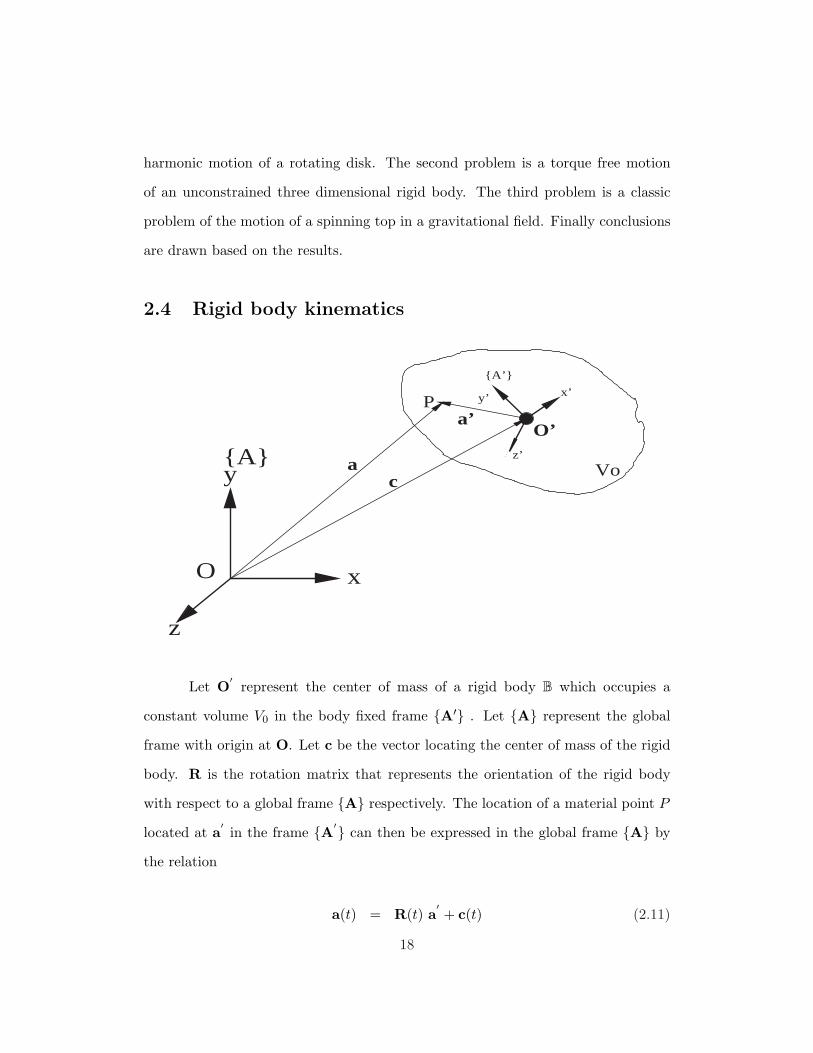
2.4 Rigid body kinematics
O x
y
z
A
A’
x’y’
z’
P
Voc
a
a’O’
Let O′
represent the center of mass of a rigid body B which occupies a
constant volume V0 in the body fixed frame A′ . Let A represent the global
frame with origin at O. Let c be the vector locating the center of mass of the rigid
body. R is the rotation matrix that represents the orientation of the rigid body
with respect to a global frame A respectively. The location of a material point P
located at a′in the frame A′ can then be expressed in the global frame A by
the relation
a(t) = R(t) a′+ c(t) (2.11)
18

where R(t) is a 3×3 rotation matrix which represents the rotation of the rigid body
(frame A′) with respect to the global frame. With the understanding that the
rotation is a function of time, unless otherwise mentioned, the explicit indication of
time dependence shall be abandoned in favor of a more compact notation R. The
vector c(t) locates the center of mass position of the rigid body in the global frame
A. The rotation matrix is expressed in terms of four Euler parameters. Specifi-
cally, R(e0, e1, e2, e3) can be decomposed as a product two rectangular matrices [53]
R = E GT where (2.12)
E =
−e1 e0 −e3 e2
−e2 e3 e0 −e1
−e3 −e2 e1 e0
and (2.13)
G =
−e1 e0 e3 −e2
−e2 −e3 e0 e1
−e3 e2 −e1 e0
(2.14)
Let the angular velocity of the rigid body expressed in the frame A′ be ω0
=[ωx′ , ωy′ , ωz′
]T. Let e = [e0, e1, e2, e3]
T represent a 4×1 vector of Euler parameters.
The angular velocity is related to the Euler parameters by the following identity [53]:
ω′= 2 G e = −2 Ge (2.15)
19
2.5 Equations of motion
2.5.1 Kinetic energy
The kinetic co-energy T ∗ can in general be expressed as
T ∗ =12
∫
Vρ a
′ · a′ dV (2.16)
Substituting equation (2.11) into (2.16), the kinetic energy can be divided into
three contributions.
T ∗ = T ∗1 + T ∗2 + T ∗3 (2.17)
where
T ∗1 =12
∫
V0
cT cρdV (2.18)
T ∗2 =∫
V0
cTRa′ρdV (2.19)
T ∗3 =12
∫
V0
(Ra
′)T (Ra
′)ρdV (2.20)
Equation (2.18) represents the translational kinetic energy and can be simplified as
T ∗1 =12m cT c (2.21)
where ‘ m ’ is the total mass of the rigid body defined as
m =∫
V0
ρdV (2.22)
20

T ∗2 represents the kinetic energy due to coupling between translation and
rotational motions. From the definition of the center of mass, the body fixed coor-
dinates of the rigid body can be computed as
a′cg =
1m
∫
V0
a′ρ dV (2.23)
The coupling kinetic energy can then be expressed in terms of the center of mass
coordinates as
T ∗2 = m cT R a′cg (2.24)
Note that
R = Rω′
(2.25)
where ω′is 3x3 skew symmetric form of the three component vector ω
′. Substituting
equation (2.25) into equation (2.24),
T ∗2 = m cT R ω′a′cg (2.26)
If the center of mass of the rigid body is chosen as a reference point (i.e the origin
of the body fixed frame coincides with the center of mass of the rigid body) then
the coupling energy T ∗2 vanishes.
T ∗2 = 0 (2.27)
T ∗3 represents the rotational kinetic energy of the rigid body about point O′. Substi-
21

tuting equation (2.25) into equation (2.20), the expression for the rotational kinetic
energy can be written as
T ∗3 =12
∫
V0
ρa′T (
Rω′)T (
Rω′)
a′dV (2.28)
=12
∫
V0
ρ(ω′a′)T (
ω′a′)
dV (2.29)
=12
∫
V0
ρ(−ω
′a′)T (
−ω′a′)
dV (2.30)
=12ω′T
(∫
V0
ρa′T a
′dV
)ω′
(2.31)
=12ω′T
J′ω′
(2.32)
where a′
is the skew symmetric matrix of the three component vector a′. The
symmetric matrix J′
is the inertia tensor of the rigid body expressed in the body
fixed frame and is defined as
J′
=∫
V0
ρa′ ⊗ a
′dV (2.33)
or
J′
=
Jx′x′ Jx′y′ Jx′z′
Jy′x′ Jy
′y′ Jy
′z′
Jz′x′ Jz
′y′ Jz
′z′
(2.34)
Substituting equation (2.15) into equation (2.32), the kinetic co-energy can be ex-
22
pressed as
T ∗3 = 2 eT GT J G e (2.35)
Using the identity
G e = −G e (2.36)
equation (2.35) can be rewritten as
T ∗3 = 2 eT GT J G e (2.37)
Let the four component angular momenta he be defined as
he =∂T ∗3∂e
(2.38)
= 4 GT J G e (2.39)
Let h′be the three component angular momenta defined in the standard form
h′= J ω
′(2.40)
Substituting equation (2.40) into equation (2.39)
he = 2 GT h′
(2.41)
Multiplying both sides of the above equation by G and noting that GTG = I
23
(identity matrix), the inverse relation can be written as
h′
=12G he (2.42)
Legendre transformation of equation (2.17), then yields kinetic energy in terms of
the center of mass momenta p and the distributed momenta h′
T =[p · c + h
′ · ω′]− T ∗ (2.43)
=12
[m−1pTp + h
′TJ′−T
h′]
(2.44)
Substituting equation (2.42) into equation (2.44), equation (2.44) can be rewritten
as
=12m−1pTp +
18he
T GTJ′−T
Ghe (2.45)
2.5.2 Potential energy
The potential energy is a function of the position and orientation of the rigid
body and can be written in functional form as
V = V (c, e0, e1, e2, e3) (2.46)
2.5.3 Non-conservative forces
Any generalized force that cannot be derived from a potential function ap-
pears explicitly on the right hand side in the equations of motion. Forces due to
friction, time varying forcing functions, and forces arising due to nonholonomic con-
straints are some examples of non-conservative forces.
24

2.5.4 Hamilton’s equations
The Hamiltonian of the system is the sum of kinetic and potential energies.
Π = T + V = Π(p,h′e, c, e) (2.47)
The Hamilton’s equations in canonical form are
p = −∂Π∂c
+ Qpnc (2.48)
c =∂Π∂p
(2.49)
he = −∂Π∂e
+ Qnc (2.50)
e =∂Π∂he
(2.51)
Next, we introduce a Lagrange multiplier λ to satisfy the following equality con-
straint,
eTe = 0 (2.52)
The term ∂Π∂e on the right hand side of equation (2.50) can be simplified as follows
∂Π∂e
=∂T
∂e+
∂V
∂e(2.53)
= −4 GT J Ge +∂V
∂e(2.54)
25

= −2 GT J(−ω
′)+
∂V
∂e(2.55)
= 2 GT h′+
∂V
∂e(2.56)
Differentiating equation (2.42) with respect to time on both sides one obtains
h′
=12
Ghe + Ghe
(2.57)
=12
4 G GT J G e + Ghe
(2.58)
=12
2 G GT h
′+ Ghe
(2.59)
Substituting equation (2.50) into equation (2.59), equation (2.59) can be rewritten
as
h′
=12
[2 G GT h
′+ G
−∂Π
∂e+ λe + Qext
](2.60)
where
Qext = Qnc − λ e (2.61)
Substituting equation (2.56) into equation (2.60) results in
h′
=12
[2 G GT h
′+ G
−2 GT h
′ − ∂V
∂e+ λe + Qext
](2.62)
Using the identities
26

(i)
G e = 0 (2.63)
(ii)
Ω′
= 2GGT = −2GGT (2.64)
where Ω′is the skew symmetric matrix
Ω′
=
0 −ωz′ ωy′
ωz′ 0 −ωx
′
−ωy′ ωx′ 0
(2.65)
equation (2.62) can be simplified as
h′
= −Ω′h′ − 1
2G
∂V
∂e+
12GQext (2.66)
Simplification of equation (2.51) results in
e =12
GT ω′
(2.67)
Summarizing, the Hamilton’s equations of motion can be written as
p = −g + Qpnc (2.68)
c = m−1p (2.69)
27

h′
= −Ω′h′ − 1
2G
∂V
∂e+
12GQext (2.70)
e =12
GT ω′
(2.71)
2.6 Thermo-mechanical coupling
Most literature on analytical dynamics includes an extensive discussion of
Hamilton’s principle and Lagrange’s and Hamilton’s equations for general three di-
mensional motion of rigid bodies. However the model development typically ignores
any thermo-mechanical coupling. The Hamilton’s equations derived in the previous
section can be extended to include thermal effects.
For a thermo-mechanical system, the appropriate stored energy potential
is the internal energy U . The stored energy function is in general a function of
the mass density ρ and entropy of density the system s. The Hamiltonian for a
thermo-mechanical system is
Π = T + U = Π(p,h′, c, ρ, s) (2.72)
Entropy evolution equations of the form
S = Sirr (2.73)
can be introduced, where Sirr is the rate of irreversible entropy production, calcu-
lated from the energy dissipation rate (W )
Sirr =(
1Θ
)W (2.74)
28

where Θ is the temperature of the rigid body.
For viscous damping effects, the energy dissipation rate is given by
W = fp · c + τh′· ω′
(2.75)
where fp and τ h′define the viscous force due to translation and rotation respectively.
2.6.1 Hamilton’s equations
The canonical form of Hamilton’s equations can be written as
p = −∂Π∂c
+ Qpnc (2.76)
c =∂Π∂p
(2.77)
he = −∂Π∂e
+ Qnc (2.78)
e =∂Π∂he
(2.79)
0 = −∂Π∂S
+ Qs (2.80)
Note that equations (2.76-2.79) are the same as equations (2.48-2.51). Let γ be the
Lagrange multiplier associated with equation (2.73), then
Qs = γ (2.81)
Qpnc = −
( γ
Θ
)fp + f c (2.82)
Qnc = −( γ
Θ
)τ h
′+ λ e + τ c (2.83)
29
In the above equations, f c and τ c arise from the mechanical constraints. Equa-
tion (2.80) requires that Θ = Qs. In other words, the Lagrange multiplier corre-
sponding to equation (2.73) is the thermodynamic temperature. Finally Hamilton’s
equations for a thermo-mechanical system can be written as
p = −g + fp + f c (2.84)
c = m−1p (2.85)
h′ = −12
G τ −Ω′h′+
12
G
τ h′+ τ c
(2.86)
e =12
GT ω′
(2.87)
S = Sirr (2.88)
2.7 Numerical examples
The preceding results are used to solve the following example problems.
2.7.1 Single degree of freedom system
Consider a rigid circular disk of radius ‘ r ’ rotating about a fixed point ‘ O ’.
Let x′, y
′and z
′form a right handed coordinate system in the body fixed frame
A′ with its origin at ‘ O ’. A linear spring is connected between point ‘ P ’ on the
disk and ground, as shown in the figure (2.2). The coordinates of the point ‘ P ’ in
the body fixed frame and global frame are (x′, y
′, z′) and (x, y, z) respectively. The
30

Pr
φ
Figure 2.2: Circular disk with a spring
orientation of the disk with respect to the global frame A is given by
[x y z
]T
= R[
x′
y′
z′
]T
(2.89)
where R is the rotation matrix. Although the use of Euler parameters seems to be
unnecessary for this problem, their use serves to verify the formulation.
2.7.2 Equations of motion
The coordinates of the point ‘ P ’ in the global frame are related to the
coordinates in the body fixed frame by the relation
[xp yp zp
]T
= R[
x′p y
′p z
′p
]T
(2.90)
31
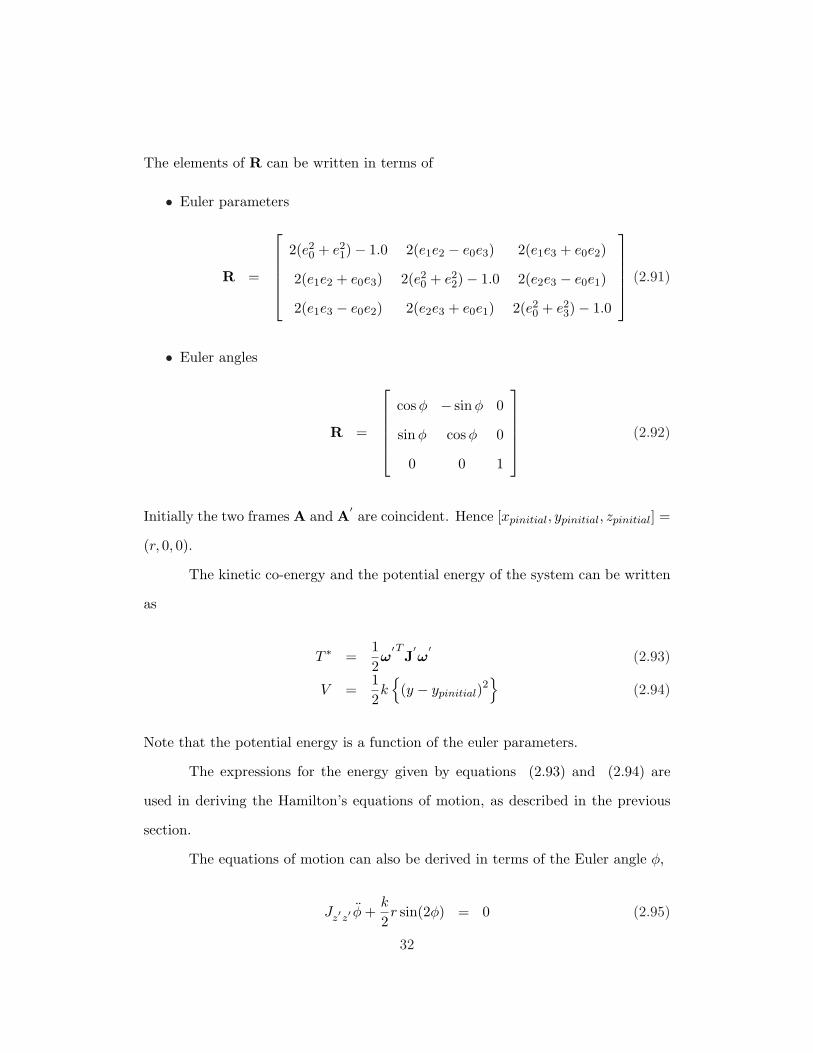
The elements of R can be written in terms of
• Euler parameters
R =
2(e20 + e2
1)− 1.0 2(e1e2 − e0e3) 2(e1e3 + e0e2)
2(e1e2 + e0e3) 2(e20 + e2
2)− 1.0 2(e2e3 − e0e1)
2(e1e3 − e0e2) 2(e2e3 + e0e1) 2(e20 + e2
3)− 1.0
(2.91)
• Euler angles
R =
cosφ − sinφ 0
sinφ cosφ 0
0 0 1
(2.92)
Initially the two frames A and A′are coincident. Hence [xpinitial, ypinitial, zpinitial] =
(r, 0, 0).
The kinetic co-energy and the potential energy of the system can be written
as
T ∗ =12ω′T
J′ω′
(2.93)
V =12k
(y − ypinitial)
2
(2.94)
Note that the potential energy is a function of the euler parameters.
The expressions for the energy given by equations (2.93) and (2.94) are
used in deriving the Hamilton’s equations of motion, as described in the previous
section.
The equations of motion can also be derived in terms of the Euler angle φ,
Jz′z′ φ +k
2r sin(2φ) = 0 (2.95)
32
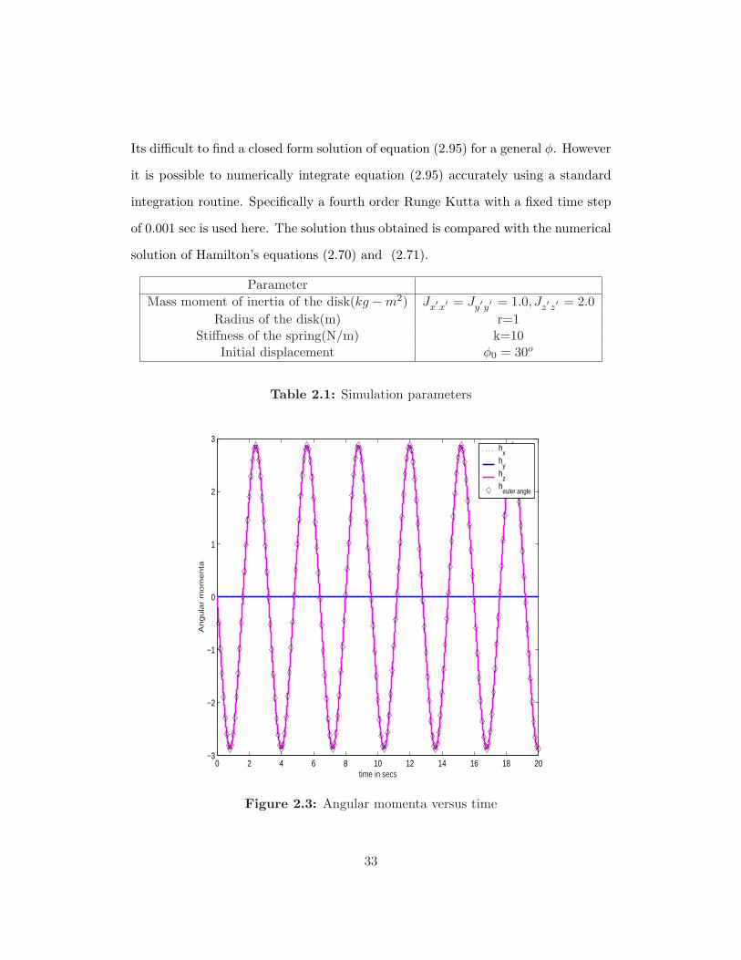
Its difficult to find a closed form solution of equation (2.95) for a general φ. However
it is possible to numerically integrate equation (2.95) accurately using a standard
integration routine. Specifically a fourth order Runge Kutta with a fixed time step
of 0.001 sec is used here. The solution thus obtained is compared with the numerical
solution of Hamilton’s equations (2.70) and (2.71).
ParameterMass moment of inertia of the disk(kg −m2) Jx′x′ = Jy′y′ = 1.0, Jz′z′ = 2.0
Radius of the disk(m) r=1Stiffness of the spring(N/m) k=10
Initial displacement φ0 = 30o
Table 2.1: Simulation parameters
0 2 4 6 8 10 12 14 16 18 20−3
−2
−1
0
1
2
3
time in secs
An
gu
lar
mo
me
nta
hx
hy
hz
heuler angle
Figure 2.3: Angular momenta versus time
33

0 2 4 6 8 10 12 14 16 18 200
0.5
1
1.5
2
2.5
time
PEKEPE
euler angleKE
euler angle
0 2 4 6 8 10 12 14 16 18 20−1
0
1x 10
−11
time
Pe
rce
nta
ge
err
or
in E
ne
rgy
Figure 2.4: Total energy and percentage error in energy versus time
0 2 4 6 8 10 12 14 16 18 20−0.5
0
0.5
1
time in secs
Eu
ler
pa
ram
ete
rs
e0e1e2e3
Figure 2.5: Euler parameters versus time
34

0 2 4 6 8 10 12 14 16 18 20−1
0
1
2
3
4
5x 10
−12
time
Perc
enta
ge e
rror
in e
ule
r para
mete
r constr
ain
t
Figure 2.6: Percentage error in euler parameter constraint time
Simulation results shown in figures (2.3) and (2.4) show good agreement
between the numerical solution of equation (2.95) and the numerical solution of
Hamilton’s equations using Euler parameters developed in this chapter.
2.7.3 Torque free motion of a rigid body
The specific problem selected here is the one analyzed by Morton [40]. The
equations of rotational motion of a torque free rigid body are simulated using the
Hamiltonian equations derived earlier. The model is conservative. The simulation
parameters are shown in table (2.2).
It is well known that the analytical solution for the torque free motion of
rigid body can be expressed in terms of Jacobian elliptic functions [69] [40].
Given the initial angular velocity (at time t=0) of the system, the angular
35

ParametersMass moment of inertia (Jx′x′ , Jy′y′ , Jz′z′ ) = (400, 307.808385, 200) kg −m2
Initial conditions Euler parameters e = (1, 0, 0, 0)
h′= (346.4101616, 0,−200) kg −m2rad/s
Table 2.2: Simulation parameters
momenta at any time t > 0 can be shown to be [69]
ωx′ (t) = ωmx
′Dn(T , k) (2.96)
ωy′ (t) = ωmy′Sn(T , k) (2.97)
ωz′ (t) = −ωmz′Cn(T , k) (2.98)
where the terms used in the above equations are defined as
•
ωmx′ =
√h′
2 − 2 TJz′z′
Jx′x′ (Jx′x′ − Jz′z′ )(2.99)
ωmy′ =
√√√√ h′2 − 2 TJz′z′
Jy′y′ (Jy′y′ − Jz′z′ )(2.100)
ωmz′ =
√2 TJx
′x′ − h′
2
Jz′z′ (Jx′x′ − Jz′z′ )(2.101)
• h′= ||h′ || = ||J′ω′ || represents the constant angular momentum. || || is the
standard Euclidean norm
36

• T = ω′T
J′ω′is the constant kinetic energy of the rigid body
• Let Γ and Γ′be defined as
Γ =
√√√√(h′
2 − 2 T Jz′z′)(
Jx′x′ − Jy′y′)
Jx′x′Jy′y′Jz′z′(2.102)
Γ′
=
√√√√(2 T Jx′x′ − h′
2)(
Jy′y′ − Jz′z′)
Jx′x′Jy
′y′Jz
′z′
(2.103)
The elliptic modulus ‘ k ’ in equations (2.96) through (2.98) is defined as
k =Γ′
Γ(2.104)
• T is defined as
T = Γ t (2.105)
• Sn, Cn and Dn are Jacobian elliptic functions. Note that
Sn2(T , k) + Cn2(T , k) = 1 (2.106)
Dn2(T , k) + k2Sn2(T , k) = 1 (2.107)
For the parameters defined in the table (2.2), the amplitudes of the angular momenta
and the elliptic modulus expressed in equations (2.96 - 2.98) can be computed to be
•[hmx′ , hmy′ , hmz′
]= [346.4102, 365.447, 200] kg-m2 rad/s
• k = 0.882948
37

The period parameter K(k) can be computed as
K(k) =∫ π
2
0
1√(1− k2 sin2 θ
) dθ (2.108)
= 2.213195 (2.109)
The period of Sn(T , k) and Cn(T , k) is
(4 K
Γ
)= 18.6786 sec (2.110)
and that of Dn(T , k) is
(2 K
Γ
)= 9.3393 sec. (2.111)
Also the minimum value of hx′ can be computed to be
min
h′x
= hmx′
(1− k2
) 12 (2.112)
= 162.6296 kg m2 rad/s (2.113)
The torque-free motion of a rigid body is calculated numerically using a fourth order
Runge Kutta integrator with a fixed time step of 0.0625 sec. Table (2.3) shows a
comparison between numerical and exact values. It can be seen that the simulation
results are in good agreement with the derived analytical results.
38

exact numericalhmx′ 346.4102 kg −m2rad/s 346.38 kg −m2rad/shmy
′ 365.447 kg −m2rad/s 365.44 kg −m2rad/s
hmz′ 200.0 kg −m2rad/s 199.975 kg −m2rad/sPeriod of hx′ 9.3393 sec 9.35 secPeriod of hy′ 18.6786 sec 18.68 secPeriod of hz′ 18.6786 sec 18.68 sec
Minimum value of h′x 162.6296 kg m2 rad/s 162.6342 kg m2 rad/s
Table 2.3: Comparison between experimental and simulation results
0 2 4 6 8 10 12 14 16 18 20−400
−300
−200
−100
0
100
200
300
400
time in secs
An
gu
lar
mo
me
nta
hx h
y a
nd
hz
hxhyhz
Figure 2.7: Angular momenta versus time
39

2 4 6 8 10 12 14 16 18 20
249.996
249.998
250
250.002
250.004
250.006
time
Kinetic Energy
Figure 2.8: Total energy versus time
0 2 4 6 8 10 12 14 16 18 20−4.5
−4
−3.5
−3
−2.5
−2
−1.5
−1
−0.5
0x 10
−5
time
Perc
enta
ge e
rror
in E
nerg
y
Figure 2.9: Percentage error in total energy versus time
40

0 2 4 6 8 10 12 14 16 18 20−1
−0.8
−0.6
−0.4
−0.2
0
0.2
0.4
0.6
0.8
1
time in secs
Eu
ler
pa
ram
ete
rs
e0
e1
e2
e3
Figure 2.10: Euler parameters versus time
0 2 4 6 8 10 12 14 16 18 20−2
−1.5
−1
−0.5
0
0.5
1
1.5
2x 10
−6
time
Perc
enta
ge e
rror
in c
onst
rain
t
Figure 2.11: Percentage error in euler parameter constraint versus time
41

0 2 4 6 8 10 12 14 16 18 200
20
40
60
80
100
120
140
160
180
time
Eu
ler
an
gle
s φo
θo a
nd
ψo
φθψ
Figure 2.12: Euler angles versus time
2.7.4 Motion of a spinning top in a gravitational field
In this example numerical simulation of the motion of a symmetrical top
spinning in a uniform gravitational field is performed using the formulation derived
earlier in this chapter. Specifically, this problem is presented as a numerical example
by Simo and Wong [66].
This is a classical problem, a description of which can be found in many
standard advanced dynamics texts [25] [24] [23] [3]. Consider a symmetrical top of
total weight ‘ W ’ rotating about its apex ‘ O ’ on a horizontal plane. Let a represent
the global frame and a′be a body fixed frame with its origin located at the center
of mass G of the top as shown in figure (2.13).
The angular velocity of the top represented in the frame of the body is ω′.
Let ‘ l ’ be the distance to the center of mass from ‘ O ’ along axis z′. The distributed
mass moment of inertia of the top about the center of mass is J′. The apex does
42

z’
y’
x’
y
z
x
O
G
a
a’
Figure 2.13: Spinning top
not translate and is in continuous contact with the horizontal plane. The kinetic
and potential energies of the system can be written as
T =12
ω′T
J′ω′
(2.114)
V = W Zg (2.115)
In the equation (2.115) ‘ W ’ is the weight of the top and Zg is the Z coordinate
of the point ‘ g ’ in the global frame. The body fixed frame is related to the global
frame by a rotation matrix. Specifically,
a = Ra′
(2.116)
43
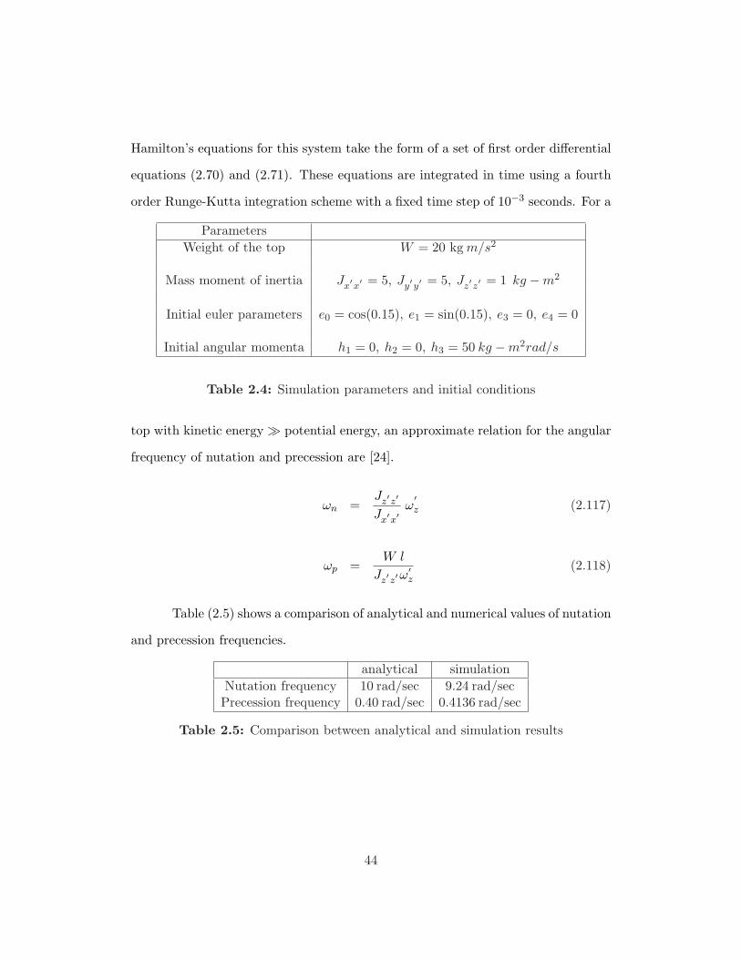
Hamilton’s equations for this system take the form of a set of first order differential
equations (2.70) and (2.71). These equations are integrated in time using a fourth
order Runge-Kutta integration scheme with a fixed time step of 10−3 seconds. For a
ParametersWeight of the top W = 20 kg m/s2
Mass moment of inertia Jx′x′ = 5, Jy′y′ = 5, Jz′z′ = 1 kg −m2
Initial euler parameters e0 = cos(0.15), e1 = sin(0.15), e3 = 0, e4 = 0
Initial angular momenta h1 = 0, h2 = 0, h3 = 50 kg −m2rad/s
Table 2.4: Simulation parameters and initial conditions
top with kinetic energy À potential energy, an approximate relation for the angular
frequency of nutation and precession are [24].
ωn =Jz′z′
Jx′x′
ω′z (2.117)
ωp =W l
Jz′z′ω′z
(2.118)
Table (2.5) shows a comparison of analytical and numerical values of nutation
and precession frequencies.
analytical simulationNutation frequency 10 rad/sec 9.24 rad/secPrecession frequency 0.40 rad/sec 0.4136 rad/sec
Table 2.5: Comparison between analytical and simulation results
44

0 2 4 6 8 10 12 14 16 18 201250
1250.1
1250.2
1250.3
time
kin
etic e
ne
rgy
0 2 4 6 8 10 12 14 16 18 201269.1066
1269.1067
1269.1067
1269.1067
1269.1068
time
tota
l e
ne
rgy
0 2 4 6 8 10 12 14 16 18 2018.8
18.9
19
19.1
19.2
time
po
ten
tia
l e
ne
rgy
Figure 2.14: Energy versus time
0 2 4 6 8 10 12 14 16 18 2050
50.02
50.04
time
||h
||
Angular momenta norm
Figure 2.15: Norm of the angular momenta versus time
45

0 2 4 6 8 10 12 14 16 18 20−0.5
0
0.5
1
time
h/||h
||
X componentY componentZ component
Figure 2.16: Spatial components of the angular momentum
0 2 4 6 8 10 12 14 16 18 20−0.5
0
0.5
1
time
Ce
nte
r o
f m
ass lo
ca
tio
n
X componentY componentZ component
Figure 2.17: Center of mass location
46

0 2 4 6 8 10 12 14 16 18 20−1
−0.5
0
0.5
1
time in secs
Eu
ler
pa
ram
ete
r e
0
0.5 1 1.5 2 2.5 3 3.5 4−1
−0.5
0
0.5
time in secs
Eu
ler
pa
ram
ete
r e
0
Figure 2.18: Euler parameter e0 versus time
0 2 4 6 8 10 12 14 16 18 20−0.5
0
0.5
time in secs
Eu
ler
pa
ram
ete
r e
1
0.5 1 1.5 2 2.5 3 3.5 4
−0.4
−0.2
0
0.2
0.4
time in secs
Eu
ler
pa
ram
ete
r e
1
Figure 2.19: Euler parameter e1 versus time
47

0 2 4 6 8 10 12 14 16 18 20−0.5
0
0.5
time in secs
Eu
ler
pa
ram
ete
r e
2
0.5 1 1.5 2 2.5 3 3.5 4−0.4
−0.3
−0.2
−0.1
0
0.1
0.2
time in secs
Eu
ler
pa
ram
ete
r e
2
Figure 2.20: Euler parameter e2 versus time
0 2 4 6 8 10 12 14 16 18 20−1
−0.5
0
0.5
1
time in secs
Eu
ler
pa
ram
ete
r e
3
0.5 1 1.5 2 2.5 3 3.5 4
−0.5
0
0.5
time in secs
Eu
ler
pa
ram
ete
r e
3
Figure 2.21: Euler parameter e3 versus time
48

−0.4−0.2
00.2
0.4
−0.4−0.2
00.2
0.40.94
0.95
0.96
X position of the center of massY position of the center of mass
Z p
ositio
n o
f th
e c
en
ter
of
ma
ss
−0.4 −0.3 −0.2 −0.1 0 0.1 0.2 0.3 0.4−0.4
−0.2
0
0.2
0.4
X position of the center of mass
Y p
ositio
n o
f th
e c
en
ter
of
ma
ss Initial position of the center
of mass of the top[0 −0.2955 0.9553]
Figure 2.22: Motion of the center of mass of the top
49
2.8 Conclusions
In this chapter, a robust Hamiltonian formulation to model rigid body dy-
namics is developed. The present formulation makes use of Euler parameters to
parameterize rotation, eliminating singularity problems associated with many three
parameter representations of rotation. Unlike previous work [40], [52], [51] the dy-
namic equations of rotational motion are devoid of any explicit Lagrange multiplier
used to enforce the Euler parameter constraint. This results in a set of first order
nonlinear ordinary differential equations which can be integrated using a standard
integration routine. The results from the numerical simulations show good agree-
ment with analytical results.
50

Chapter 3
A general hybrid particle-finite
element modeling methodology
for hypervelocity impact
3.1 Introduction
The drawbacks of a pure particle or a pure mesh based method to model
hypervelocity impact have been described in chapter (1). In this chapter a hybrid
model, which combines the strengths of both particle and standard Lagrangian
finite elements to model hypervelocity impact of orbital debris on space structures
is developed.
Most particle methods including smooth particle hydrodynamics(SPH) and
the particle in cell method (PIC) treat particles as moving interpolation points.
Fahrenthold and Koo [17] proposed an alternative particle model based on Hamil-
ton’s equations. The continuum is discretized into physical particles which trans-
late, deform and interact with each other thermo-mechanically. Fahrenthold and
51

Horban [20] extended this work by coupling the aforementioned particle model with
Lagrangian finite elements. This provided the ability to model strength effects while
retaining all the advantages of a particle based model. Further the model was en-
hanced to capture plasticity and continuum damage and fragmentation behavior
commonly seen in hypervelocity impact. A thermodynamically consistent contin-
uum damage and fragmentation model [15] was developed for this purpose. The
formulation was implemented in a three dimensional computer code. A disadvan-
tage of the above formulation is the use of a penalty method to model contact-
impact. Recognizing this fact Fahrenthold and Koo [18] developed a hybrid particle
finite element model, using a kernel function for density interpolation. An explicit
distinction is made between nearest and non-nearest neighbors. This distinction
is reflected in the use of two different kernels to compute density. The continuum
is discretized into particles and elements simultaneously with all the mass lumped
into particles. This results in an inconsistent mass matrix [46]. Fahrenthold and
Horban [19] extended the above formulation by incorporating plasticity, continuum
damage and a fragmentation model.
3.2 Overview of the modeling methodology
The current work generalizes the hybrid particle-finite element work of Fahren-
thold and Horban [19]. The continuum is discretized simultaneously but not re-
dundantly into particles and finite elements. Particles are used to model inertia
effects and thermo-mechanical volumetric response. Elements are used to model
inter-particle tensile forces and elastic-plastic shear. Thus particles and elements
are used to model different physical effects in the same continuum. The particles
can translate and rotate in three dimensional space and interact with each other
thermo-mechanically. The three dimensional rotational motion of the particles are
52
described in terms of the Euler parameters. The use of ellipsoidal particles gives the
modeling methodology a unique feature, modeling geometries with a high aspect ra-
tio. In addition, this offers a possibility of reducing computer resource requirements
in some hypervelocity simulations. A kernel function is used for density interpola-
tion, eliminating the need to explicitly impose any mass conservation properties on
the kernel. The chosen kernel function is singular and satisfies exact Lagrangian
kinematics. Unlike previous work [20] the density kernel is a function of the particle
separation distance and the rotational parameters. Rotational dynamics developed
in chapter (2) are used to model three dimensional rotational dynamics of the par-
ticles. The large deformation finite element kinematics used by Fahrenthold and
Horban [20] are extended to include hexahedra with arbitrary aspect ratios.
The model uses the plasticity formulation developed by Fahrenthold and
Horban [15]. Damage to the continuum is modeled with the introduction of two
scalar damage variables. Standard to many hydrocodes, the model introduces arti-
ficial viscosity and artificial heat flux to model shocks and to damp the translational
mode of the particles.
The model development presented here adopts an energy based approach.
The classical approach of using a weighted residual scheme is abandoned in favor
of a system dynamics method. Hamiltonian mechanics forms the basis for model
development. The Hamiltonian for the thermo-mechanical system can be obtained
from the kinetic and internal energy expressions for the system. The Hamiltonian of
the system is a function of the generalized coordinates and the generalized momenta,
commonly referred to as states. Simple differentiation operations of the Hamiltonian
function, with respect to the state variables, yield the governing equations for the
dynamics of the system. The rate equations for the internal state variables result in a
set of nonholonomic constraints. Lagrange multipliers (determined in closed form)
53
are used to embed these constraints, resulting in a set of first order differential
equations. Once a set of initial conditions are specified, these equations can be
integrated numerically using a standard integration scheme.
The rest of the chapter is organized as follows. First the particle and element
kinematics are established, following which the interpolation function for density is
developed. Expressions for kinetic and internal energy are developed subsequently.
The kinetic and internal energy define the Hamiltonian for the thermo-mechanical
system. Conservative forces are obtained by differentiating the Hamiltonian with
respect to the generalized displacements. A plasticity model is developed which
introduces the plastic deformation as a state variable. Damage variables are intro-
duced to model loss of strength of the continuum. Artificial viscosity and artificial
heat flux expressions are developed to model shocks. The coupling of mechanical
and thermal domains is achieved with the introduction of entropy as a state variable.
Using the aforementioned development the state equations are derived, which are
a set of first order nonlinear ordinary differential equations. Other computational
issues such as neighbor finding and time step calculations are discussed. Initial
validation of the model is performed by simulating a one dimensional wall shock
problem. Comparison of numerical and exact solutions are presented. The vali-
dated model is used to solve more complex impact problems. A discussion of results
from these simulations concludes the chapter.
3.3 Kinematics
3.3.1 Particle kinematics
The system being modeled here is discretized into a set of ‘ n ’ non-deforming
ellipsoidal particles, each with a fixed mass m(i), (i = 1, 2, 3, . . . , n) and a distributed
54

mass moment of inertia expressed in the body fixed frame of J′(i). The particles
translate and rotate in three dimensional space and interact with each other thermo-
mechanically. The translational velocity of the center of mass of a particle is c(i)
and the angular velocity of a particle represented in the frame of the particle is ω′(i).
The total particle entropy is S(i).
Particles are used to model contact-impact and volumetric effects while La-
grangian finite elements are used to model tension, elastic shear forces and plasticity
effects. Elements are formed by connecting the nodal coordinates of the particles.
Though particles and elements are used simultaneously, they are used to model
different physical effects in the same continuum.
3.3.2 Element kinematics
The center of mass coordinates of the particles serve as nodes of the finite
elements. In three dimensional simulations, the particles are packed according to a
body centered cubic packing scheme. The eight corner nodes define hexahedra. The
body centered node is associated with six sets of four particles (representing the
faces of the hexahedra) to form sub-elements. The Jacobians of the sub-elements
are used to determine inter-particle tensile forces, while shear forces are calculated
using the hexahedra. The deviatoric strain tensor E(j) of an element ‘ j ’ is defined
as
E(j) =12
C(j) − I
where (3.1)
C(j) = J (j)− 23 C(j) and (3.2)
J (j) =
det(C(j)
) 12 (3.3)
55

‘ J (j) ’ is the Jacobian of the hexahedron, ‘ C(j) ’ is the right Cauchy-Green strain
tensor and ‘ I ’ is the second order identity tensor.
Although the current model uses body centered packing scheme, the mod-
eling framework is general enough to allow alternate packing schemes and finite
element interpolation functions.
3.3.3 Density Interpolation
The mass density of a particle is obtained by using a density interpolation
of the form
ρ(i) = ρ0(i) + ρ(i) (3.4)
where ‘ ρ0(i) ’ is the constant reference density of the particle and ‘ ρ(i) ’ is the density
contribution from all other particles
ρ(i) =n∑
j=1
j 6=i
ρ0(j)W (i,j) (3.5)
with ‘ n ’ the total number of particles in the system.
Kernel function
The kernel function W (i,j) in equation (3.5) is chosen to be a positive semi-
definite function such that it models the exact Lagrangian kinematics of the particles
under uniform compression. This interpolation scheme for the density ensures that
the density of an isolated particle cannot drop below its reference density ‘ ρ0 ’.
W (i,j) =
(1
ζ(i, j)
)3
− 1
H
α
(ρ(i)0
ρ(i)
) 13
− ζ(i, j)
(3.6)
56

where H[x− δ] represents the standard heaviside function defined as
H[x− δ] = 1 if x ≥ δ and
= 0 otherwise (3.7)
‘ α ’ is a scalar constant which depends on the dimension of the problem and the
packing scheme chosen. For three dimensional problems with body centered cubic
packing, α = 12
(1 + 2
√3
3
). Note that the kernel function defined by equation (3.6)
is implicit, in that the argument of the heaviside function in equation (3.6) depends
on the density ratio. This dependence mimics the true physical behavior in the
sense that a particle which is highly compressed due to its immediate neighbors is
partially screened from interacting with other particles. ζ(i, j) in equation (3.6) is
defined as follows.
Let the effective interaction distances along the three principal axes be de-
fined as
heff1 = 2 β(j) h(j)1 (3.8)
heff2 = 2 β(j) h(j)2 (3.9)
heff3 = 2 β(j) h(j)3 (3.10)
where h(j)1 , h
(j)2 and h
(j)3 are the semi-axes lengths of the ellipsoid centered at c(j).
β(j) is a constant packing factor. Let A(j) be a 3× 3 diagonal matrix defined as
A(j) =
h2eff1 0 0
0 h2eff2 0
0 0 h2eff3
−1
(3.11)
57

Let R(j) be the rotation matrix that transforms global components of a vector
into components in the frame of the particle ‘ j ’. As discussed in chapter (2),
the elements of the rotation matrix R(j) can be represented in terms of the Euler
parameters of the jth particle.
R(j) =
e0(j)2 + e1
(j)2 − e2(j)2 − e3
(j)2 2(e1(j)e2
(j) + e0(j)e3
(j))
2(e1(j)e2
(j) − e0(j)e3
(j)) e0(j)2 − e1
(j)2 + e2(j)2 − e3
(j)2
2(e1(j)e3
(j) + e0(j)e2
(j)) 2(e2(j)e3
(j) − e0(j)e1
(j))
2(e1(j)e3
(j) − e0(j)e2
(j))
2(e2(j)e3
(j) + e0(j)e1
(j))
e0(j)2 − e1
(j)2 − e2(j)2 + e3
(j)2
(3.12)
ζ(i, j) is can then be defined by the following equation
ζ(i,j) =(
c(i) − c(j))T
R(j)TA(j)R(j)(c(i) − c(j)
) 12
(3.13)
Unlike density kernels used in smooth particle hydrodynamics [47], the den-
sity interpolation function described here is non-dimensional and has compact sup-
port. Fahrenthold and Koo [18] and Fahrenthold and Horban [20] distinguish be-
tween the density contributions from nearest and non-nearest neighbors by using
two different non-dimensional kernels. A singular kernel was used for density con-
tributions from nearest neighbors. The form of this kernel function was chosen such
that it modeled exact Lagrangian kinematics under uniform compression of the par-
ticles. A second density kernel was used for density contributions from non-nearest
neighbors. In chapter (4) advanced simulation and validation results based on these
kernels is presented.
58

In the present formulation no explicit distinction is made between nearest and
non-nearest neighbors. One singular non-dimensional kernel with adaptive support
given by equation (3.6) is used for all the particles.
3.4 Kinetic Energy
The kinetic co-energy T ∗ of the system is given by
T ∗ =n∑
i=1
T ∗(i) (3.14)
where
T ∗(i) =12m(i)c(i)T c(i) +
12ω′(i)TJ
′(i)ω′(i) (3.15)
The linear and angular momenta can be defined as
p(i) =∂T ∗
∂c(i)= m(i)c(i) (3.16)
h′(i) =
∂T ∗
∂ω′(i) = J′(i)ω
′(i) (3.17)
A standard Legendre transformation of equation (3.14) results in an expression for
kinetic energy which depends on the center of mass momenta p(i) and the distributed
momenta h′(i)
T =
n∑
i=1
[p(i) · c(i) + h
′(i) · ω′(i)]
− T ∗ or (3.18)
T =12
n∑
i=1
[p(i)T m(i)−1
p(i) + h′(i)TJ
′(i)−Th′(i)
](3.19)
59

Using equation (2.45), equation (3.19) can be rewritten as
T =n∑
i=1
[12
p(i)T m(i)−1p(i) +
18
he(i)T G(i)T J(i)′−T
G(i) he(i)
](3.20)
3.5 Internal Energy
The appropriate stored potential function for the thermo-mechanical system
considered here is the internal energy. The internal energy depends in general on
the kinematics and the chosen equation of state.
U =∫
Vρ u (ρ, s, c, d, D,Ee) dV (3.21)
where ‘ ρ ’ and ‘ s ’ are the density and the entropy per unit mass previously defined,
computed at the center of mass ‘ c ’ of the particle. The scalars ‘ D ’ and ‘ d ’
represent volumetric and deviatoric damage variables. The exact evaluation of the
integral in equation (3.21) is in general not possible. In a later part of this section,
a discrete form of the equation (3.21) is developed.
The internal energy can be decomposed into two primary parts.
U = Uparticles + Uelements (3.22)
The energy stored in the particles depends on the chosen equation of state and can
be written in functional form as
Uparticles =n∑
i=1
m(i)u(i)(ρ(i), s(i)
)(3.23)
where ‘ u ’ is the internal energy per unit mass and ‘ s ’ is the entropy per unit mass.
The present formulation is general enough to incorporate various equations of state.
60
Uelements can be written as
Uelements =
ne∑
j=1
ns∑
k=1
12
(1−D(j)
)V
(j,k)0 κ(j)
(J (j,k) − 1
)2
H
[J (j,k) − 1
]
+
ne∑
j=1
(1− d(j)
)V
(j)0 µ(j)Ee(j):Ee(j)
(3.24)
where ‘ ne ’ is the number of elements, ‘ ns ’ is the number of sub-elements per
element, ‘ κ(j) ’ is the element bulk modulus, ‘ J (j) ’ and ‘ J (j,k) ’ are the element
and sub-element Jacobians and ‘ V(j)0 ’ and ‘ V
(j,k)0 ’ are the reference volumes of
the element and the subelements. Also ‘ µ(j) ’ is the element shear modulus and
‘ : ’ is a double contraction operator. The elements are used to model inter-particle
tensile and elastic shear forces. Although the present model assumes a linear elastic
response, the modelling frame work is general enough to accommodate more complex
non-linear elastic material behavior.
‘ D(j) ’ and ‘ d(j) ’ are normal and deviatoric scalar damage variables respec-
tively, associated with element ‘ j ’. The damage variables vary from zero to one,
with zero representing an intact element and one representing a complete failure of
the element. The evolution equations for damage will be discussed in section (3.8).
The element Jacobian and the elastic strain tensor are a function of the
nodal coordinates of the finite element. The nodal coordinates are the center of
mass coordinates of the particles. Hence
J (j,k) = J (j,k)(c(i)) (3.25)
Ee(j) = Ee(j)(c(i),Ep(j)) (3.26)
61
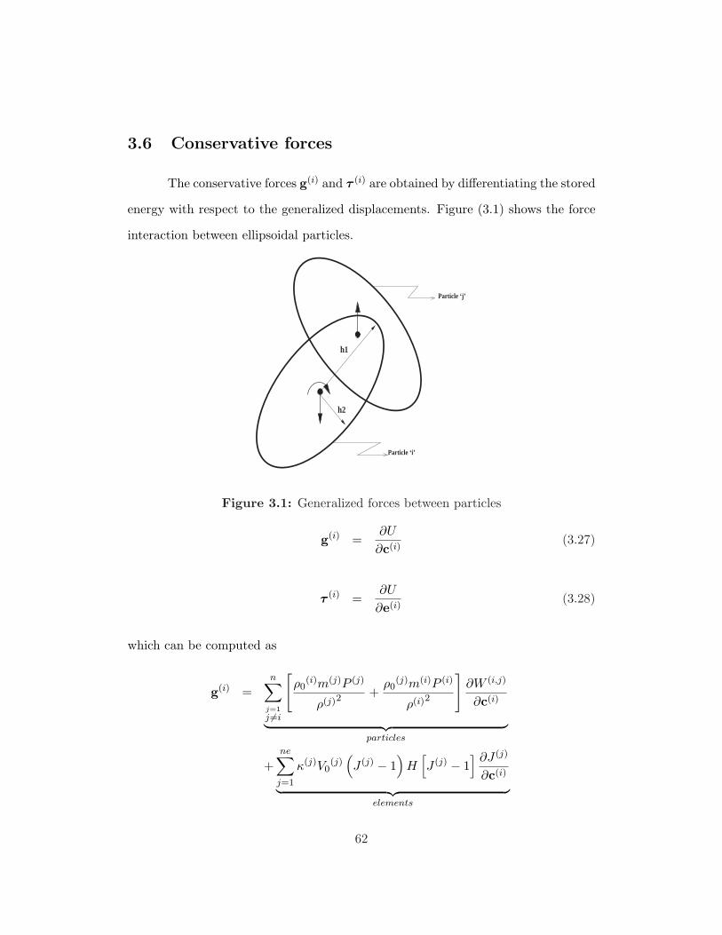
3.6 Conservative forces
The conservative forces g(i) and τ (i) are obtained by differentiating the stored
energy with respect to the generalized displacements. Figure (3.1) shows the force
interaction between ellipsoidal particles.
h1
h2
Particle ‘j’
Particle ‘i’
Figure 3.1: Generalized forces between particles
g(i) =∂U
∂c(i)(3.27)
τ (i) =∂U
∂e(i)(3.28)
which can be computed as
g(i) =n∑
j=1
j 6=i
[ρ0
(i)m(j)P (j)
ρ(j)2+
ρ0(j)m(i)P (i)
ρ(i)2
]∂W (i,j)
∂c(i)
︸ ︷︷ ︸particles
+ne∑
j=1
κ(j)V0(j)
(J (j) − 1
)H
[J (j) − 1
] ∂J (j)
∂c(i)
︸ ︷︷ ︸elements
62

+ne∑
j=1
2µ(j)V0(j)E(j) :
∂E(j)
∂c(i)
︸ ︷︷ ︸elements
(3.29)
τ (i) =n∑
j=1
j 6=i
[ρ0
(i)m(j)P (j)
ρ(j)2
]∂W (j,i)
∂e(i)(3.30)
The first term in equation (3.29) is the contribution by all other ‘ n − 1 ’ particles
on particle ‘ i ’. The thermodynamic pressure ‘ P ’ and temperature ‘ Θ ’ depend on
the chosen equation of state and are defined as
P (i) = ρ(i)2 ∂u(i)
∂ρ(i)(3.31)
Θ(i) =∂u(i)
∂s(i)(3.32)
The second and last terms in equation (3.29) are contributions from the elements.
Equation (3.30) represents a 4× 1 generalized torque vector.
3.7 Plasticity model
The present formulation uses the plasticity model developed by Fahrenthold
and Horban [15]. Plastic deformation is assumed to take place at constant vol-
ume. The model assumes an additive decomposition of elastic and plastic deviatoric
strains.
E(j) = Ee(j) + Ep(j) (3.33)
63

The right Cauchy-Green plastic deformation tensor Cp is related to the plastic strain
tensor Ep by the expression
Cp(j) = I + 2 Ep(j) (3.34)
or
Ep(j) =12C
p(j)(3.35)
The assumption of isochoric plastic deformation and the fact that “plastic
dissipation” has to be a positive semi-definite quantity (which follows from second
law of thermodynamics) imposes the constraints
For the isochoric constraint
det(Cp(j)
)= 1 (3.36)
or
det(Cp(j)
)(Cp(j)
)−1: Cp(j)
= 0 (3.37)
Substituting equation (3.35) into the above equation yields,
(Cp(j)
)−1: Ep(j) = 0 (3.38)
For positive dissipation
− ∂U
∂Ep(j): Ep(j) ≥ 0 (3.39)
64
The partial derivative in equation (3.39) defines the energy conjugate to the
plastic strain Ep(j), a second order stress tensor S(j).
S(j) = − 1V0
(j)
∂U
∂Ep(j)(3.40)
= 2µ(j)(1− d(j))[E(j) −Ep(j)
](3.41)
3.7.1 Flow rule
The plasticity model used here is based on an incremental plastic strain
formulation and makes use of a non-associative flow rule.
∆Ep(j) = ∆λ(j)W(j) (3.42)
The stress term W(j) in equation (3.42) is so chosen that the flow law satisfies the
isochoric constraint represented by equation (3.36)
W(j) = Cp(j)S(j) + S(j)Cp(j) − 13
tr [Cp(j)S(j) + S(j)Cp(j)] I (3.43)
S(j) is the second order stress tensor defined previously in equation (3.40) and Cp(j)
is the right Cauchy-Green deformation tensor defined by equation (3.34). ‘ tr ’
denotes the trace operator. ∆λ is a scalar which will be defined later.
Let τ (j) be a scalar measure of the effective stress defined as
τ (j) =[12
(S(j) : S(j)
)] 12
(3.44)
The yield stress Y (j) is in general a function of the initial yield stress, thermal
65
softening, and kinematic hardening and can be expressed as
Y (j) = (1− d(j))
Y(j)0 (1 + β
(j)0 εp(j))n(j)
1− β
(j)2 ΘH(j)
(3.45)
In the equation (3.45), Y(j)0 is the initial yield stress, εp(j) is the effective plastic
strain computed by integrating
εp(j) =[12
(Ep(j) : Ep(j))] 1
2
(3.46)
β(j)0 is the (constant) hardening modulus and n(j) is the (constant) hardening ex-
ponent. The temperature ΘH(j) is defined by the relation
ΘH(j) =
(Θ(j)
max −Θ(j)0
)(Θ(j)
m −Θ(j)0
) (3.47)
where
Θ(j)0 = Reference temperature,
Θ(j)m = Melt temperature and
Θ(j)max = Maximum temperature
∆λ(j) in equation 3.42 is a positive scalar quantity defined by
∆λ(j) =(τ (j) − Y (j)) H(τ (j) − Y (j))
(1− d(j)) 2 µ(j)o
(3.48)
3.8 Damage evolution
Damage mechanics and classical fracture mechanics provide the necessary
tools to model the loss of strength of materials and other non-continuum effects, like
66

fracture and fragmentation. However the complexity of using fracture mechanics
concepts like the J-integral or the crack opening displacement in a finite strain
plasticity setting has favored the use of damage mechanics [42].
Central to the theory of damage mechanics is the concept of a “damage vari-
able”. The use of damage variables provides a mechanism to progressively degrade
material properties. The damage variable can be a scalar or an appropriate higher
order tensor.
In this formulation, two scalar damage variables ‘ D ’ and ‘ d ’ are used to
model the loss of strength of the material, in tension and shear respectively. The
damage values are initially set to zero, which represents an intact material. The
modeling methodology is general enough to incorporate both rate dependent (e.g
Grady-Kipp) and rate independent damage evolution schemes. The present work
uses a rate independent damage evolution model given by
∆D(j) = Λ maxH[σ(j) − σsp(j)],H[εp(j) − εf(j)],
H[P (j) − P c(j)],H[τ (j) − Y (j)] (3.49)
∆d(j) = Λ maxH[σ(j) − σsp(j)],H[εp(j) − εf(j)],
H[P (j) − P c(j)],H[τ (j) − Y (j)] (3.50)
Λ is a constant chosen to be 0.1. This means that damage variables are evolved over
ten time steps, after the element has failed due to any of the following
• The tensile pressure P (j) drops below a specified value P c(j)
• Effective shear stress τ (j) exceeds a predefined value Y (j)
• The maximum eigenvalue of the deviatoric stress σ(j)exceeds a specified value
σsp(j)
67
• The accumulated plastic strain εp(j)has reached a specified value εf(j)
When the damage value reaches 1.0 the element has lost strength and Λ is reset to
zero.
Unlike some finite element based codes, the energy released due to dam-
age evolution goes into irreversible entropy production. This provides a means to
rigorously conserve energy.
3.9 Artificial viscosity
Consistent with the general practice in shock physics, the present modeling
methodology introduces artificial viscosity to
• Model shocks
• Damp the translational mode of the particles
The viscous damping force due to the relative particle velocity is
f (i) =n∑
j=1
γ(i,j)(c(i) − c(j)
)H
[−
(c(i) − c(j)
)·(c(i) − c(j)
)](3.51)
where the damping coefficient γ(i,j) is given by
γ(i,j) =12co
(ρ(i)cs
(i)A(i) + ρ(j)cs(j)A(j)
)×
[1.0− ζ(i, j)] H [1.0− ζ(i, j)] (3.52)
‘ co ’ is a dimensionless numerical damping coefficient, c(i)s is the local speed of the
sound in the material and A(i) is the cross-sectional area of the particle. The heav-
iside functions in equation (3.51) and (3.52) ensure that viscous force acts only on
particles which are moving towards each other.
68

3.10 Artificial heat flux
Most hydrocodes use a conduction model to allow heat (generated due to
viscous effects) to diffuse through the material. Consistent with this practice, the
present formulation makes use of an entropy based heat conduction model of the
form
Scon(i) =1
Θ(i)
n∑
j=1
Υ(i,j)(Θ(i) −Θ(j)
)(3.53)
where the heat conduction coefficient Υ(i,j) is defined as
Υ(i,j) =12k0
ρ(i)cs
(i)cv(i)A(i) + ρ(j)cs
(j)cv(j)A(j)
×
[1.0− ζ(i, j)] H [1.0− ζ(i, j)]
‘ k0 ’ is the constant coefficient of heat conduction of the material and ‘ cv ’ is the
specific heat capacity. The heaviside function ensures that conduction occurs only
between contacting particles.
3.11 Entropy as a state
The use of an entropy variable couples the mechanical and thermal energy
domains. Since entropy is introduced here as a state it is essential to specify an
evolution equation that determines the entropy of the system at any instant in
time. A general entropy evolution equation for particle ‘ i ’ is written in the form
S(i) = Sirr(i) − Scon(i) (3.54)
69

where Sirr(i) is the irreversible entropy evolution due to energy dissipation and
Scon(i) is the entropy evolution due to heat conduction. The irreversible entropy
evolution rate is given by the expression
Sirr(i) =1
Θ(i)ν(i) (3.55)
The dissipative power ν(i) in equation (3.55) can be decomposed into contributions
from three main sources
ν(i) = ν(i)viscous + ν
(i)plastic + ν
(i)damage (3.56)
The viscous power ν(i)viscous in equation (3.56) is due to energy dissipation via artificial
viscosity, described in section (3.9), and can be expressed as
ν(i)viscous = f (i) · c(i) (3.57)
The power dissipated in damage evolution ν(i)damage is given by
ν(i)damage =
n(i)e∑
j=1
1np
Γd(k(i,j))d(k(i,j)) + ΓD(k(i,j))D(k(i,j))
(3.58)
where ‘ np ’ is the number of particles per element, ‘ n(i)e ’ is the number of elements
associated with particle ‘ i ’ and k(i,j) is the element associated with the ith particle.
ΓD(j) and Γd(j) are the rate at which energy is released during damage evolution,
given by
ΓD(j) = − ∂U
∂D(j)(3.59)
70

Γd(j) = − ∂U
∂d(j)(3.60)
The power dissipated in plastic flow is given by
ν(i)plastic =
n(i)e∑
j=1
1npS(k(i,j)) : Ep(k(i,j)) V
(j)0 (3.61)
S(k(i,j)) is the second Kirchoff-Piola deviatoric stress tensor defined by equation (3.40).
3.12 State equations
In the earlier sections, expressions for the internal energy and kinetic energy
were developed. The Hamiltonian for the thermo-mechanical system is defined as
the sum of the kinetic and internal energies.
Π = T + U = Π(p(i), c(i),he
(i), e(i), S(i), d(j), D(j),Ep(j))
(3.62)
Hamilton’s canonical equations can then be written as
p(i) = − ∂Π∂c(i)
+ qc(i)(3.63)
c(i) =∂Π
∂p(i)(3.64)
he(i)
= − ∂Π∂e(i)
+ qe(i)(3.65)
e(i) =∂Π
∂he(i)
(3.66)
71

0 = − ∂Π∂S(i)
+ qS(i)(3.67)
0 = − ∂Π∂D(j)
+ qD(j)(3.68)
0 = − ∂Π∂d(j)
+ qd(j)(3.69)
0 = − ∂Π∂Ep(j)
+ qp(j)(3.70)
Equations (3.63) and (3.64) represent the translational state equations, (3.65) through
(3.66) represent the rotational motion of the particles, (3.67) represents entropy
evolution, (3.68) and (3.69) represent damage evolution and (3.70) represents the
equation for the evolution of plastic strain.
qc(i), qS(i)
, qD(j), qd(j)
, qp(j)are the generalized nonconservative forces which
are determined by the nonholonomic constraints (3.57), (3.58) and (3.61). The
above equations are supplemented by the evolution equations for S(i), d(j), D(j)
and Ep(j). Lagrange multipliers are introduced to apply the nonholonomic con-
straints (3.54). Specifically,
qc(i)= −
(γS(i)
ΘS(i)
)f (i) (3.71)
qS(i)= γS(i)
(3.72)
qD(j)= γD(j) − ΓD(j) 1
np
np∑
i=1
(γS(k(j,i))
Θk(j,i)
)(3.73)
72

qd(j)= γd(j) − Γd(j) 1
np
np∑
i=1
(γS(k(j,i))
Θk(j,i)
)(3.74)
qp(j)= Gp(j) − V0
(j)S(j)
np∑
i=1
(γS(k(j,i))
Θk(j,i)
)(3.75)
Equation (3.67) forces the Lagrangian multiplier qS(i) to be equal to the temperature
Θ(i). This results in a simplification of equations (3.71) through (3.75).
Equations (3.65) and (3.66) model the rotational dynamics of the particles.
Simplification of these equations follow from the results in section (2.5.4) of chap-
ter (2).
The aforementioned simplifications result in the final form Hamilton’s equa-
tions
p(i) = −g(i) − f (i) (3.76)
c(i) =1
m(i)p(i) (3.77)
h′(i) = −Ω
′(i)h′(i) − 1
2G(i)τ (i) (3.78)
e(i) =12G(i)T ω
′(i) (3.79)
S(i) = Sirr(i) − Scon(i) (3.80)
D(j) = D(ρ(i), s(i), c(i), D(j), d(j),Ep(j)
)(3.81)
73

d(j) = d(ρ(i), s(i), c(i), D(j), d(j),Ep(j)
)(3.82)
Ep(j) = λ(j)
12W(j)T : W(j)
− 12
W(j) (3.83)
3.13 Computational Issues
3.13.1 Integration routine
Hamilton’s equations are a set of first order differential equations, which can
be integrated using a standard integration routine. In the present work an explicit,
variable time step, second order Runge-Kutta routine is used. The time step is
computed from the system characteristic frequencies. Specifically
∆t =(
1c4
)1√
wmaxwhere (3.84)
wmax = max
w(i)k , k = 1, 2, . . . , 5 and i = 1, 2, 3, . . . , np
(3.85)
c4, is a dimensionless constant, w(i)k are the squared frequencies given by
w(i)k = |pnet
k |/(m(i)hmin); k = 1, 2, 3 (3.86)
w(i)4 = p(i)2/(m(i)hmin) (3.87)
w(i)5 = |Snet|/(m(i)c(i)
v )2
(3.88)
pnetk is the net rate of change of linear momenta and is given by the right hand side
of equation (3.76), and Snet is the net rate of change of entropy evolution given by
equation (3.80). hmin is the minimum of the semi-major lengths of the ellipsoidal
74
particles, given by
hmin = min
h(i)1 , h
(i)2 , h
(i)3 , i = 1, 2, 3, . . . , n
(3.89)
3.13.2 Neighbor search
Equations (3.5), (3.29), (3.30), (3.51) and (3.53) involve summations over
‘ (n− 1) ’ particles and in general require an O(n2) computational effort. However,
an efficient nearest neighbor finding algorithm provides a significant saving in com-
putational cost. The current formulation uses linked lists [33] to reduce the number
of particles which contribute to the summation. Alternative techniques based on
tree search methods can also be used.
3.13.3 Parallel Implementation
Three dimensional simulation of hypervelocity impact phenomena requires
large amounts of memory and CPU time. With the emergence of massively parallel
computers, there has been a significant change in the way in which hypervelocity
impact computations are performed. The model developed here is implemented in
parallel using OpenMP compiler directives. A more detailed discussion is provided
in section (4.4) of chapter (4)
3.14 Examples
3.14.1 Initial validation
One dimensional wall shock problem
Initial validation of the model is done by solving a one dimensional wall shock
problem [55] using an ideal gas equation of state with density shift. The expressions
75

for the internal energy u(i), pressure P (i) and temperature Θ(i) of particle ‘ i ’ are
u(i) = cv
(Θ(i) −Θ0
)(3.90)
P (i) = (γ − 1)cvΘ(i)(ρ(i) − ρ0
)(3.91)
Θ(i) = Θ0 exp
[(s(i) − s0
)
cv
][ρ(i)
ρ0
](γ−1)
exp[(γ − 1)
(ρ0
ρ(i)− 1
)](3.92)
where cv is the specific heat at constant volume, γ is the ratio of specific heats, s0 is
the reference entropy, ρ0 is the reference density, and Θ0 is the reference temperature.
This problem can be treated as a benchmark problem to test codes in shock
physics. In this problem, response of a stream of particles (ideal gas) to shock
compression is studied. The shock is generated by impact of the particles with a
rigid wall, located at x = 1.25 cm. The system consists of ‘ 201 ’ particles uniformly
distributed over the region 0 < x < 2.5 cm. The number of finite elements is ‘ 200 ’.
The initial conditions for the simulation i.e at ‘ t = 0 ’ are,
ρ(i) = 1.0 g/cm3 (3.93)
s(i) = 1.0 Mb− cm3/(g − oK) (3.94)
c(i) =
+1.0 cm/µs for x < 0
−1.0 cm/µs for x > 0(3.95)
Since this example problem is one dimensional, there is no rotation of the particles.
Equations (3.76) through (3.83) are integrated using a second order Runge-Kutta
algorithm. The simulation parameters are given in table (3.1).
The exact post-shock solution [12] for this problem can be obtained by application
76
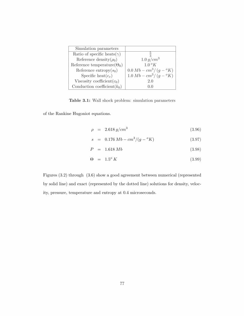
Simulation parametersRatio of specific heats(γ) 5
3Reference density(ρ0) 1.0 g/cm3
Reference temperature(Θ0) 1.0 oKReference entropy(s0) 0.0 Mb− cm3/ (g − oK)
Specific heat(cv) 1.0 Mb− cm3/ (g − oK)Viscosity coefficient(c0) 2.0
Conduction coefficient(k0) 0.0
Table 3.1: Wall shock problem: simulation parameters
of the Rankine Hugoniot equations.
ρ = 2.618 g/cm3 (3.96)
s = 0.176 Mb− cm3/(g − oK) (3.97)
P = 1.618 Mb (3.98)
Θ = 1.5o K (3.99)
Figures (3.2) through (3.6) show a good agreement between numerical (represented
by solid line) and exact (represented by the dotted line) solutions for density, veloc-
ity, pressure, temperature and entropy at 0.4 microseconds.
77

0 0.5 1 1.5 2 2.5x
1
1.25
1.5
1.75
2
2.25
2.5
densi
ty
Figure 3.2: Exact and numerical density distribution at t = 0.4µs
0 0.5 1 1.5 2 2.5x
-1
-0.5
0
0.5
1
velo
cit
y
Figure 3.3: Exact and numerical velocity distribution at t = 0.4µs
78

0 0.5 1 1.5 2 2.5x
0
0.25
0.5
0.75
1
1.25
1.5
pre
ssure
Figure 3.4: Exact and numerical pressure distribution at t = 0.4µs
0 0.5 1 1.5 2 2.5x
1
1.1
1.2
1.3
1.4
1.5
tem
pera
ture
Figure 3.5: Exact and numerical temperature distribution at t = 0.4µs
79

0 0.5 1 1.5 2 2.5x
0
0.025
0.05
0.075
0.1
0.125
0.15
0.175
entr
opy
Figure 3.6: Exact and numerical entropy distribution at t = 0.4µs
3.14.2 Simulation with spherical particles
The model developed earlier in this chapter was numerically implemented
in the three dimensional parallel code EXOS. In this section, numerical simulations
of problems involving thermo-mechanics, elastic-plastic effects and significant dam-
age to the continuum are presented. The simulation results presented here involve
spherical particles, which are a special case of the more general model developed
earlier. Because of the inherent symmetry involved with spherical particles, there
is no rotational motion of the particles. Three simulation examples are presented,
with velocities ranging from 1 km/s to 11 km/s.
1. EXOS simulation: Depleted Uranium(DU) 0.75% Ti long rod im-
pact on a steel plate
The first example is a depleted Uranium, 0.75% Titanium long rod impacting
a steel plate. Table (3.2) shows the simulation parameters. Figures (3.7) and
80
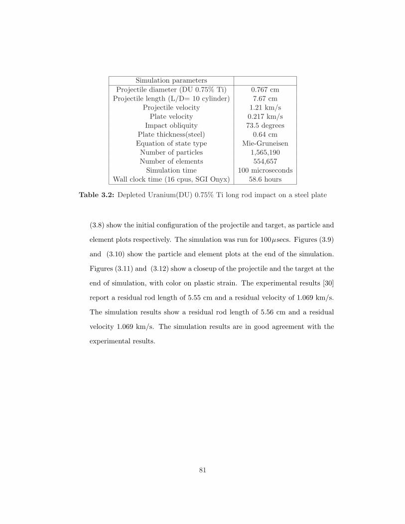
Simulation parametersProjectile diameter (DU 0.75% Ti) 0.767 cm
Projectile length (L/D= 10 cylinder) 7.67 cmProjectile velocity 1.21 km/s
Plate velocity 0.217 km/sImpact obliquity 73.5 degrees
Plate thickness(steel) 0.64 cmEquation of state type Mie-GruneisenNumber of particles 1,565,190Number of elements 554,657
Simulation time 100 microsecondsWall clock time (16 cpus, SGI Onyx) 58.6 hours
Table 3.2: Depleted Uranium(DU) 0.75% Ti long rod impact on a steel plate
(3.8) show the initial configuration of the projectile and target, as particle and
element plots respectively. The simulation was run for 100µsecs. Figures (3.9)
and (3.10) show the particle and element plots at the end of the simulation.
Figures (3.11) and (3.12) show a closeup of the projectile and the target at the
end of simulation, with color on plastic strain. The experimental results [30]
report a residual rod length of 5.55 cm and a residual velocity of 1.069 km/s.
The simulation results show a residual rod length of 5.56 cm and a residual
velocity 1.069 km/s. The simulation results are in good agreement with the
experimental results.
81
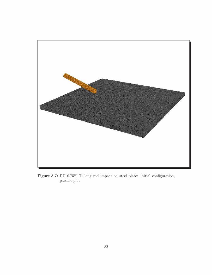
Figure 3.7: DU 0.75% Ti long rod impact on steel plate: initial configuration,particle plot
82

Figure 3.8: DU 0.75% Ti long rod impact on steel plate: initial configuration,element plot
83

Figure 3.9: DU 0.75% Ti long rod impact on steel plate: final configuration, par-ticle plot
84

Figure 3.10: DU 0.75% Ti long rod impact on steel plate: final configuration,element plot
85
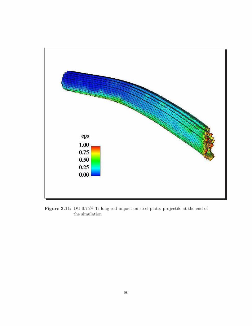
Figure 3.11: DU 0.75% Ti long rod impact on steel plate: projectile at the end ofthe simulation
86

Figure 3.12: DU 0.75% Ti long rod impact on steel plate: target at the end of thesimulation
87

2. EXOS simulation: Multi-plate shield impact, ESA benchmark case
#4
In this example, simulation of the oblique impact of a projectile on an alu-
minum double bumper system is performed. Simulation studies attempted us-
ing SPH based codes have resulted in a poor match up with the experimental
results [21]. The simulation parameters are shown in table (3.3). Figure (3.13)
Simulation parametersProjectile diameter (aluminum cylinder) 0.5062 cm
Projectile length 2.2046 cmFirst bumper thickness (aluminum plate) 0.25 cm
Second bumper thickness (aluminum plate) 0.25 cmWall thickness (aluminum plate) 0.50 cm
Bumper-to-bumper spacing 6.00 cmBumper-to-wall spacing 6.00 cm
Impact velocity 11.0 km/secImpact obliquity 45 degrees
Equation of state type SESAME 3719Number of particles 4,269,067
Total simulation time 150 microsecondsWall clock time 53.8 hours
Number of processors (SGI Origin) 256
Table 3.3: Multi-plate shield impact, ESA benchmark case #4
shows an element plot of the initial configuration. The model employed four
elements across each shield plate, eight elements across the diameter of the
cylindrical projectile and eight elements across the wall plate. The wall plate
dimensions are approximately 30 × 30 cm. Figures (3.14), (3.15) and (3.16)
show element plots at the end of 67µ secs, 94µ secs and 133µ secs. Consistent
with the experiment results, the simulation showed no wall plate perforation.
The simulation was carried further, to end at 150 µ secs. Figures (3.17) and
(3.18) show the element and particle plots at 150µsecs. The simulation showed
88

only a bulge in the wall plate.
Figure 3.13: ESA4: initial configuration, element plot
89

Figure 3.14: ESA4: element plot at t = 67 µ secs
90
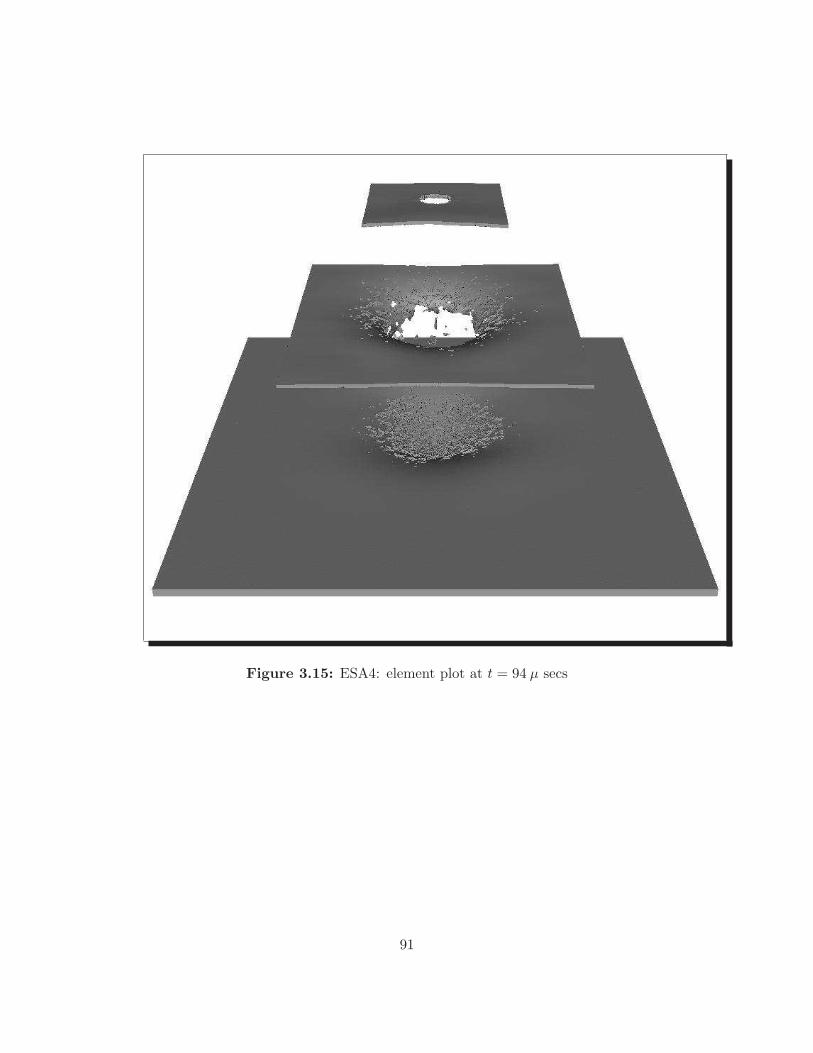
Figure 3.15: ESA4: element plot at t = 94 µ secs
91
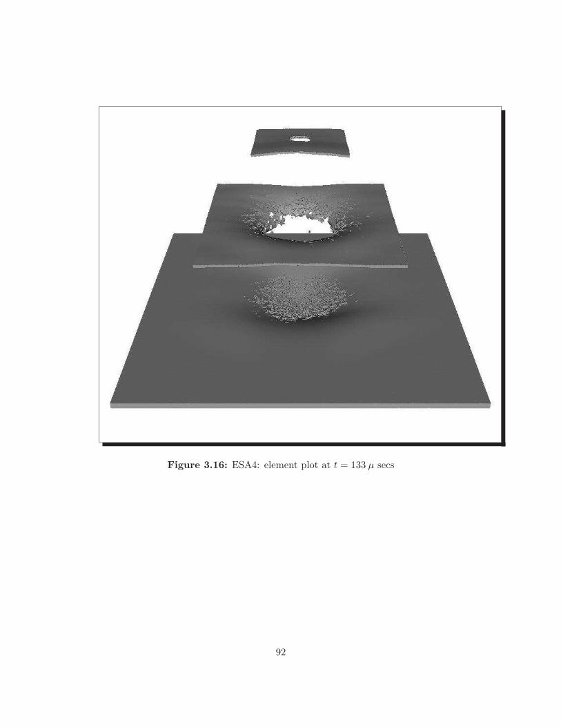
Figure 3.16: ESA4: element plot at t = 133 µ secs
92

Figure 3.17: ESA4: element plot at t = 150 µ secs
93

Figure 3.18: ESA4: particle plot at t = 150 µ secs
94

Figure 3.19: ESA4: close up element plot at t = 150 µ secs
95

Figure 3.20: ESA4: close up element plot at t = 150 µ secs
96

3. EXOS simulation: Tungsten long rod impact on a steel plate at
1.833 km/s
This example simulation involved a long cylindrical tungsten rod, LD ratio
of 20, impacting a steel plate at 1.833 km/sec. The simulation parameters
are given in table (3.4). Figure (3.21) and (3.22) show element and particle
Simulation parametersProjectile diameter (tungsten, L/D=20 cylinder) 0.475cm
Impact velocity 1.833 km/sImpact obliquity 75 degrees
Plate thickness (steel) 0.95 cmEquation of state type Mie-GruneisenNumber of particles 1,484,294Number of elements 519,009
Simulation time 150 microseconds
Table 3.4: Tungsten long rod impact on a steel plate at 1.833 km/s
plots of the initial configuration. The simulation was performed for 150µ secs.
Figures (3.23), (3.24) and (3.26) show different views of the element plot at the
end of simulation. Figure (3.25) shows a particle plot at the end of simulation.
Figures (3.27) and (3.28) show element plots, with color on plastic strain,
at the end of simulation. A comparison of the simulation and experimental
results is shown in table (3.5). The simulation results are in good agreement
with the experimental results [75].
experimental simulationRod erosion 40% 37.4%
Residual velocity 1.784 km/s 1.60 km/sPlate hole size 1.23 cm× 3.05 cm 1.67 cm (average)× 3.53 cm
Table 3.5: Comparison between experimental and simulation results
97

Figure 3.21: Tungsten long rod on a steel plate: initial configuration, element plot
98
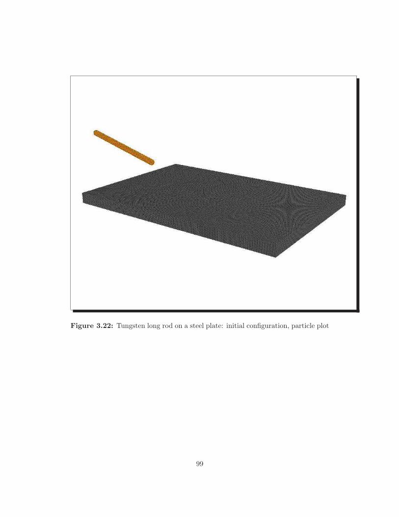
Figure 3.22: Tungsten long rod on a steel plate: initial configuration, particle plot
99
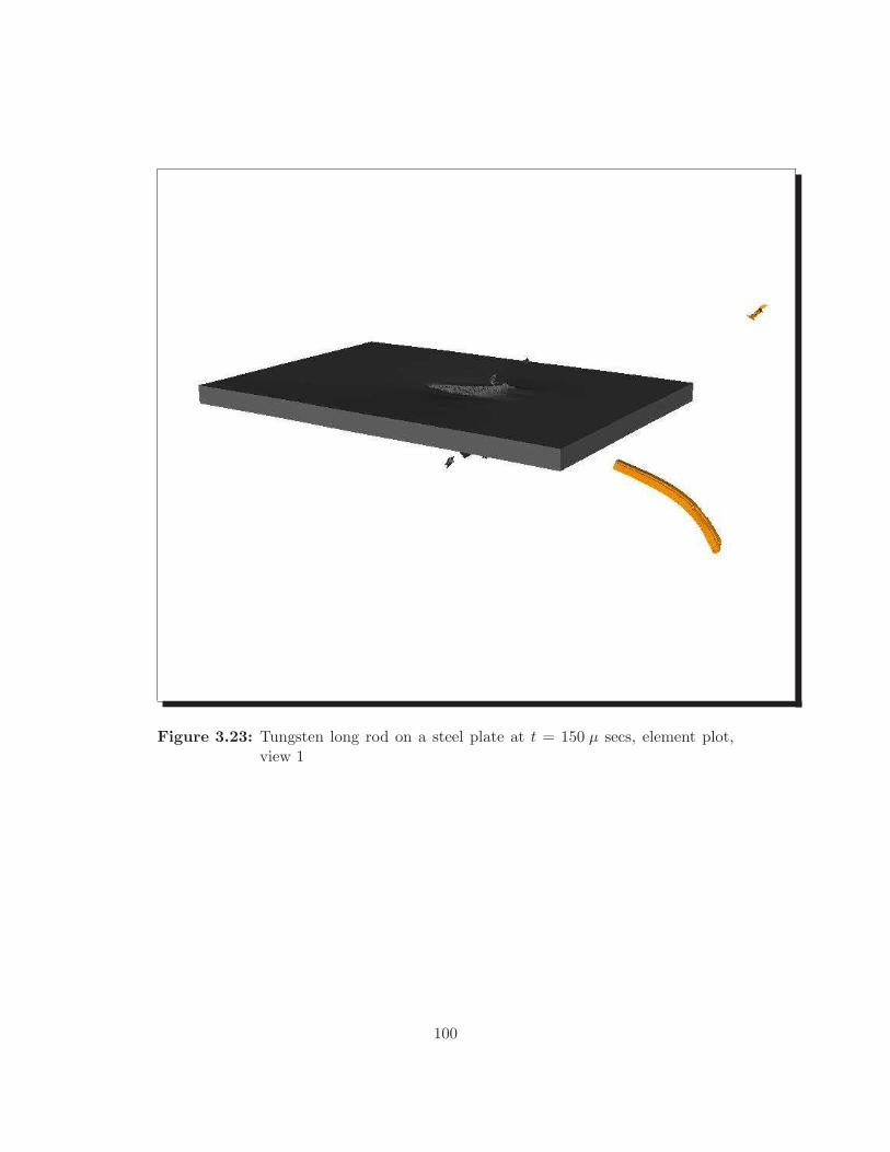
Figure 3.23: Tungsten long rod on a steel plate at t = 150 µ secs, element plot,view 1
100

Figure 3.24: Tungsten long rod on a steel plate at t = 150 µ secs, element plot,view 2
101

Figure 3.25: Tungsten long rod on a steel plate at t = 150 µ secs, particle plot
102

Figure 3.26: Tungsten long rod on a steel plate: target at t = 150 µ secs, elementplot
103
Figure 3.27: Tungsten long rod on a steel plate: projectile at t = 150 µ secs
104
Figure 3.28: Tungsten long rod on a steel plate: target at t = 150 µ secs, color onplastic strain
105

3.14.3 Simulation using ellipsoidal particles
In this section, simulation results performed using ellipsoidal particles are
presented. Four simulation examples are presented. The examples of a depleted
titanium long rod impact and tungsten long rod impact were described earlier,
using spherical particles.
1. EXOS simulation: Oblique sphere impact
The first example simulation using ellipsoidal particles involves an aluminum
sphere impacting on an aluminum plate. The parameters for the simulation
are shown in table (3.6). Ellipsoidal particles with aspect ratio of (2 : 2 : 1)
Simulation parametersProjectile diameter(sphere) 0.953 cm
Projectile velocity 6.56 km/sImpact obliquity 45 degreesPlate thickness 0.1143 cm
Equation of state type Mie-GruneisenNumber of particles 194,728
Simulation time 6.6 microseconds
Table 3.6: Oblique sphere impact
are used for the plate. Figure (3.29) and (3.30) show the initial and final
configuration. The simulation stop time is 6.6 µ secs. The simulation result is
in good agreement with the experimental radiograph [59].
106
Figure 3.29: DU 0.75% Ti long rod impact on a steel plate: Initial configuration
107
Figure 3.30: DU 0.75% Ti long rod impact on a steel plate: Initial configuration
108
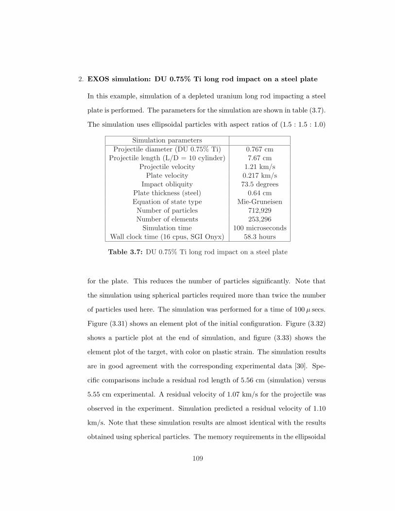
2. EXOS simulation: DU 0.75% Ti long rod impact on a steel plate
In this example, simulation of a depleted uranium long rod impacting a steel
plate is performed. The parameters for the simulation are shown in table (3.7).
The simulation uses ellipsoidal particles with aspect ratios of (1.5 : 1.5 : 1.0)
Simulation parametersProjectile diameter (DU 0.75% Ti) 0.767 cm
Projectile length (L/D = 10 cylinder) 7.67 cmProjectile velocity 1.21 km/s
Plate velocity 0.217 km/sImpact obliquity 73.5 degrees
Plate thickness (steel) 0.64 cmEquation of state type Mie-GruneisenNumber of particles 712,929Number of elements 253,296
Simulation time 100 microsecondsWall clock time (16 cpus, SGI Onyx) 58.3 hours
Table 3.7: DU 0.75% Ti long rod impact on a steel plate
for the plate. This reduces the number of particles significantly. Note that
the simulation using spherical particles required more than twice the number
of particles used here. The simulation was performed for a time of 100 µ secs.
Figure (3.31) shows an element plot of the initial configuration. Figure (3.32)
shows a particle plot at the end of simulation, and figure (3.33) shows the
element plot of the target, with color on plastic strain. The simulation results
are in good agreement with the corresponding experimental data [30]. Spe-
cific comparisons include a residual rod length of 5.56 cm (simulation) versus
5.55 cm experimental. A residual velocity of 1.07 km/s for the projectile was
observed in the experiment. Simulation predicted a residual velocity of 1.10
km/s. Note that these simulation results are almost identical with the results
obtained using spherical particles. The memory requirements in the ellipsoidal
109
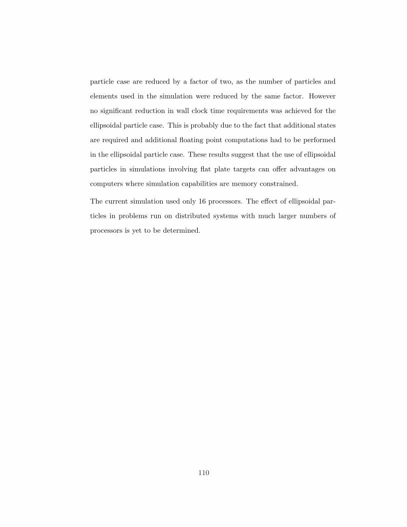
particle case are reduced by a factor of two, as the number of particles and
elements used in the simulation were reduced by the same factor. However
no significant reduction in wall clock time requirements was achieved for the
ellipsoidal particle case. This is probably due to the fact that additional states
are required and additional floating point computations had to be performed
in the ellipsoidal particle case. These results suggest that the use of ellipsoidal
particles in simulations involving flat plate targets can offer advantages on
computers where simulation capabilities are memory constrained.
The current simulation used only 16 processors. The effect of ellipsoidal par-
ticles in problems run on distributed systems with much larger numbers of
processors is yet to be determined.
110

Figure 3.31: DU 0.75% Ti long rod impact on a steel plate: Initial configuration
111

Figure 3.32: DU 0.75% Ti long rod impact on a steel plate at t = 100µ secs
112
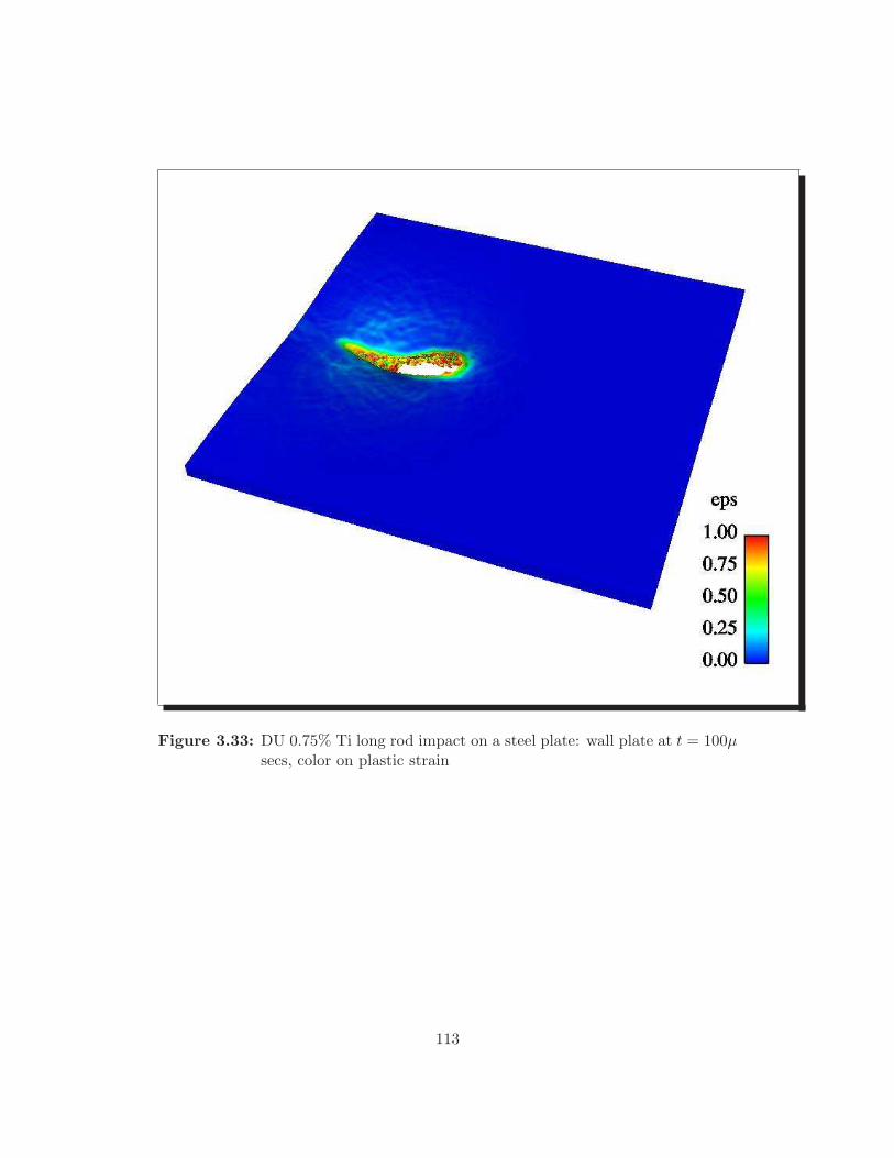
Figure 3.33: DU 0.75% Ti long rod impact on a steel plate: wall plate at t = 100µsecs, color on plastic strain
113

3. EXOS simulation: Tungsten long rod impact on a steel plate at
1.833 km/s
In this example, simulation of a tungsten long rod impacting a steel plate
is performed. Note that simulation results for this problem, using spherical
particles were presented earlier as example (3) of subsection (3.14.2). In this
section, the simulation is performed using ellipsoidal particles with an aspect
ratio of (1.5 : 1.5 : 1.0) in the plate. The simulation parameters are shown
in table (3.8). Figure (3.34) shows an element plot of the initial configura-
Projectile diameter (tungsten, L/D=20 cylinder) 0.475cmImpact velocity 1.833 km/sImpact obliquity 75 degrees
Plate thickness (steel) 0.95 cmEquation of state type Mie-GruneisenNumber of particles 671,176Number of elements 235,389
Simulation time 150 microsecondsNumber of processors (average) 12.45
Wall clock time (SGI Onyx) 87.06 hours
Table 3.8: Tungsten long rod impact on a steel plate at 1.833 km/s
tion. Figures (3.35) and (3.36) show particle and element plots respectively
at the end of simulation. The simulation stop time is 150 µ secs. The simula-
tions results are in good agreement with the experimental radiograph [75]. A
comparison of experimental and simulation results are presented in table (3.9)
experimental simulationRod erosion 40% 37.9%
Residual velocity 1.784 km/s 1.60 km/sPlate hole size 1.23 cm× 3.05 cm 1.84 cm (average)× 3.36 cm
Table 3.9: Comparison between experimental and simulation results
114

Figure 3.34: Tungsten long rod on a steel plate: initial configuration, element plot
115

Figure 3.35: Tungsten long rod on a steel plate at t = 150µ secs, particle plot
116

Figure 3.36: Tungsten long rod on a steel plate at t = 150µ secs, element plot
117

Figure 3.37: Tungsten long rod on a steel plate: projectile at t = 150µ secs
118

4. EXOS simulation: Whipple shield impact, inhibited shaped charge
projectile (SWRI test number 7139-19)
In this example problem, simulation of the impact of an inhibited shape charge
projectile on a Whipple shield is performed. This problem was run as a test
case for ellipsoidal particles. A (1.5:1.5:1.0) aspect ratio was chosen for the
particles. The simulation parameters are shown in table (3.10). Figure (3.38)
Simulation ParametersProjectile mass (aluminum cylinder) 1.38 gProjectile length-to-diameter ratio 1.4
Projectile pitch 0.0 degreesProjectile yaw 9.4 degrees
Bumper thickness (aluminum plate) 0.127 cmWall thickness (aluminum plate) 0.4826 cm
Bumper-to-wall spacing 7.62 cmImpact velocity 11.41 km/secImpact obliquity 45 degrees
Equation of state type Mie-GruneisenNumber of particles 297,372
Simulation time 30.2 microsecondsWall clock time 58.8 hours
Number of processors (SGI Onyx) 7
Table 3.10: Whipple shield impact, inhibited shaped charge projectile (SWRI testnumber 7139-19)
shows an element plot of the initial configuration, while figures (3.39) and
(3.40) show the particle and element plots respectively at the end of simula-
tion. The simulation was run for 30.2 µ secs. The simulation used only one
element across the shield plate and 10 elements across the wall plate. The
wall plate dimensions are approximately 25× 25cm. The simulation predicted
a wall plate hole dimension of 72× 62mm, versus 60× 20mm observed in the
experiment [27] [26]. This coarse model seems to overpredict the wall damage.
Moreover, the model used a Mie-Gruniesen equation of state, which might not
119

be appropriate at this high velocity.
Figure 3.38: Whipple shield impact, inhibited shaped charge projectile (SWRI test
number 7139-19) : initial configuration
120
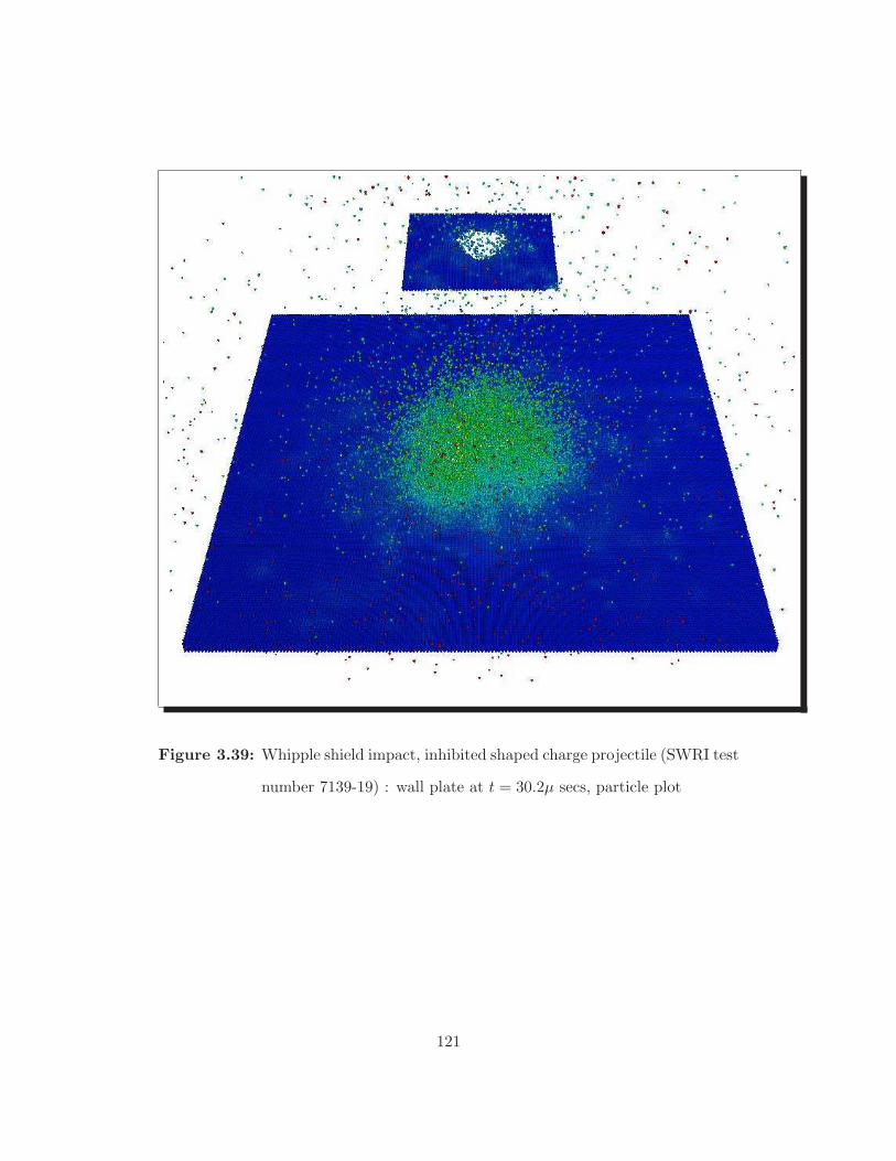
Figure 3.39: Whipple shield impact, inhibited shaped charge projectile (SWRI test
number 7139-19) : wall plate at t = 30.2µ secs, particle plot
121

Figure 3.40: Whipple shield impact, inhibited shaped charge projectile (SWRI test
number 7139-19) : wall plate at t = 30.2µ secs, element plot
122

3.15 Conclusions
In this chapter, a general hybrid particle-finite element method has been
developed to simulate high velocity impact dynamics. The following are some of the
salient features of the method.
(i) The model developed does not make use of penalty methods, diffusive grid-
particle mapping schemes (like the ones used in PIC methods), and slide-
line algorithms. Contact-impact is modeled using a non-dimensional kernel
function.
(ii) Strength is modeled using Lagrangian finite elements. No particle-element
coupling algorithm is necessary, since the finite element is embedded in the
continuum, with the centers of mass of the particles serving as nodes of the
finite elements.
(iii) A general particle model has been developed. This enables modeling of struc-
tures with aspect ratios (such as plates), resulting in significant savings in
memory requirements.
(iv) The introduction of entropy as a state variable, in an energy based frame-
work, provides an efficient way to couple thermal and mechanical domains
and provides the framework to represent energy conservation relations.
(v) The introduction of damage models ensures a smooth transition from solid
material to solid-fluid mixture, without discarding energy or mass, and without
resorting to any rezoning.
123

Chapter 4
Advanced numerical simulations
Most recent work simulating orbital debris impact effects has employed either
pure particle or mixed particle-continuum methods [29] [20] since only particle-based
kinematic schemes offer both an efficient solution to the debris propagation prob-
lem and an entirely general representation of contact-impact. Work based on pure
particle methods has encountered difficulties with accurate modelling of material
strength effects [21], and other complications [43]. It appears that some mixed or
hybrid particle-continuum method will prove most effective in meeting the need for
fundamental improvements in simulation-based design of orbital debris shielding.
This chapter describes work performed to evaluate a particular new hybrid
particle-continuum method [18], developed to simulate orbital debris impact prob-
lems. The numerical method is evaluated here, via simulation of a set of ISC launcher
experiments, the latter conducted by Grosch [27] [26] to investigate the perfor-
mance of International Space Station(ISS) shielding in oblique impacts at a velocity
of eleven kilometers per second. The simulations discussed include
• Both Whipple and multi-plate shield designs
• Both aluminum and composite shielding materials and
124
• Both hollow cylindrical projectiles (produced by the ISC launchers) and mass
equivalent spherical projectiles (for comparison to lower velocity LGG tests).
The simulations were performed using a parallel code. In addition to the
simulation results, speedup data are presented for test problems run on up to 128
processors, on an Origin 2000 system operated by the Numerical Aerospace Simu-
lation facility at NASA Ames Research Center.
4.1 Numerical method
The model used here is slightly different from the one developed in the pre-
vious chapter.
• Inertia is represented by point masses. These particles have no distributed
mass moment of inertia. The particles can only translate and interact with
each other thermo-mechanically. This is a special case of a more general model
developed in chapter (3).
• The mass density of at a particle ‘ i ’ is expressed as
ρ(i) = ρ0(i) + ρ(i) + ρ(i) (4.1)
where ρ0(i) is the constant reference density of particle ‘i’.
ρ(i) =n0∑j=1
j 6=i
ρ0(j)W0
(i,j) (4.2)
ρ(i) =n1∑j=1
j 6=i
ρ0(j)W1
(i,j) (4.3)
125
and ‘n0’ is the (fixed) number of nearest neighbors of particle ‘ i ’ in the ref-
erence configuration. The number of nearest neighbors in the reference con-
figuration in general depends on the dimension of the problem and the chosen
particle packing scheme. For a body centered cubic packing scheme, it is 2σ
where σ = 1, 2 or 3, depending on the dimension of the problem. The sum-
mation in equation (4.3) is over all other particles. Thus the total number of
particles in the system is
n = 1 + n0 + n1 (4.4)
The kernel function W(i,j)0 in equation (4.2) is chosen to reflect exact La-
grangian kinematics under uniform compression with the fixed set of nearest
neighbors.
W0(i,j) =
1n0
[(h(i) + h(j)
)
rij
]σ
− 1
H
[(h(i) + h(j)
)− rij
](4.5)
(4.6)
In the above equation, rij = |c(i) − c(j)| is the distance between the particle
centers of mass and h(i) is the effective particle radius of particle ‘ i ’, which
may differ from the particle radius at the reference density h(i)0 by a factor
β(i). This allows for closed packing of particles at the reference density.
To model collisions with non-nearest neighbors, a simple linear kernel W1(i,j)
is chosen.
W(i,j)1 =
[α(j)
β(j)σ
]1− rij
2h(j)
H
2h(j)
(ρ0
(i)
(ρ0
(i) + ρ(i))) 1
σ
− rij
(4.7)
where α is determined by forcing the kernel W1(i,j) to satisfy the following
126

relation
m(i) = ρ(i)0
∫
VW1
(i)(x− c(i), 2h(i)
)dV (4.8)
For three dimensional calculations, α(j) = 12 . Note that the argument in
the step function has a dependence on the density calculation from the nearest
neighbors. This ensures that a particle that is highly compressed due to the
nearest neighbors set is partially screened from other collisions.
4.2 Inhibited Shape charge(ISC) Launcher Simulations
This section describes simulations of four different ISC launcher experiments,
the latter performed by Grosch [27] [26] on several different debris shield configu-
rations. All of the simulations involved a projectile velocity of slightly over eleven
kilometers per second, and all but one involved a velocity vector obliquity of 45
degrees. The ISC projectiles were hollow aluminum cylinders with a length-to-
diameter ratio less than two, and had a mass of approximately one gram. Since
the projectile description was obtained from flash radiograph measurements, there
is some uncertainty in the projectile mass and geometry data.
In general the ISC projectiles exhibited both pitch and yaw with respect
to the velocity vector, hence all of the simulations reported here are fully three
dimensional. The models were composed of 100,000-500,000 particles and required
as much as four days to simulate 30-50 microseconds in physical time. The models
were run in parallel on either 7 processors of an SGI Onyx or 32 processors of an SGI
Origin, requiring up to 1GB of RAM. Computer resource constraints of course placed
limits on the simulation times and the spatial resolutions of the models. Note that
reducing the particle size by a factor of two would require a factor of eight increase
127
in the number of particles and a factor of sixteen increase in the required wall clock
time.
4.2.1 Material properties
The simulated experiments are described in detail by Grosch [27] [26]. Mate-
rial properties were estimated using data from Steinberg [68], [41], and Hiermaier
et al. [32]. Material models for the composites are the subject of current research.
Table (4.1) shows the material properties used in the simulations.
Material propertiesParameter Aluminum Nextel Kevlar
Equation of state type Mie-Gruneisen Linear LinearShear modulus (Mbar) 0.271 0.164 0.100
Reference bulk density (g/cc) 2.7 0.82021 0.741084Reference bulk modulus (Mbar) 0.7832 0.66633 0.415389
Initial yield stress (Mbar) 0.0029 0.008 0.008Maximum yield stress (Mbar) 0.0058 0.008 0.008
Strain hardening exponent 0.1 0 0Strain hardening modulus 125.0 0 0Thermal softening modulus 0.5 1.0 1.0
Melt temperature (kilodegrees Kelvin) 1.22 1.22 0.70Specific heat
(Mbar-cm3 per g-kilodegrees Kelvin) 0.00884 0.00884 0.01420Spall stress (Mbar) 0.012 0.100 0.100Plastic failure strain 2.0 0.2 0.2
First order numerical viscosity coefficient 0.01 0.01 0.01Second order numerical viscosity coefficient 1.0 1.0 1.0
Numerical conduction coefficient 0.1 0.1 0.1
Table 4.1: Material properties for the example simulations
4.2.2 Whipple shield with a stand off distance 7.62 cm
The first simulation involved a 45 degree oblique impact on an aluminum
Whipple shield at a standoff distance of 7.62 cm. The parameters for simulation are
128

shown in the table (4.2).
Simulation ParametersSWRI Test Number 7139-19
Shield type Al WhippleFirst aluminum plate thickness (cm) 0.127
Second aluminum plate thickness (cm) 0.0Wall plate thickness (aluminum, cm) 0.4826
Maximum standoff (cm) 7.62Impact velocity (km/sec) 11.41
Impact obliquity (velocity vector, deg) 45Projectile mass (aluminum, g) 1.38
Projectile length-to-diameter ratio 1.4Projectile pitch (wrt velocity vector, deg) 0Projectile yaw (wrt velocity vector, deg) 9.4
Number of particles 142,867Simulation time (µsec) 46.6Wall clock time (hours) 28.1
Average number of processors 6.9System Onyx
Table 4.2: Simulation parameters for Aluminum Whipple shield, stand off 7.62 cm
Figures (4.1) and (4.2) show particle plots at impact and at 46.6 microsec-
onds after impact, while figure (4.3) shows an element plot of intact material at the
simulation stop time. The simulation predicts a wall plate hole size (71 × 44 mm)
somewhat greater than that observed in the experiment (60 × 20 mm).
129

Figure 4.1: Whipple shield impact simulation: 7.62cm stand off distance, initialconfiguration, particle plot
130
Figure 4.2: Whipple shield impact simulation: 7.62cm stand off distance, particleplot at t = 46.6 µsec with color on temperature
131

Figure 4.3: Whipple shield impact simulation: 7.62cm stand off distance, elementplot at t = 46.6 µsec
132
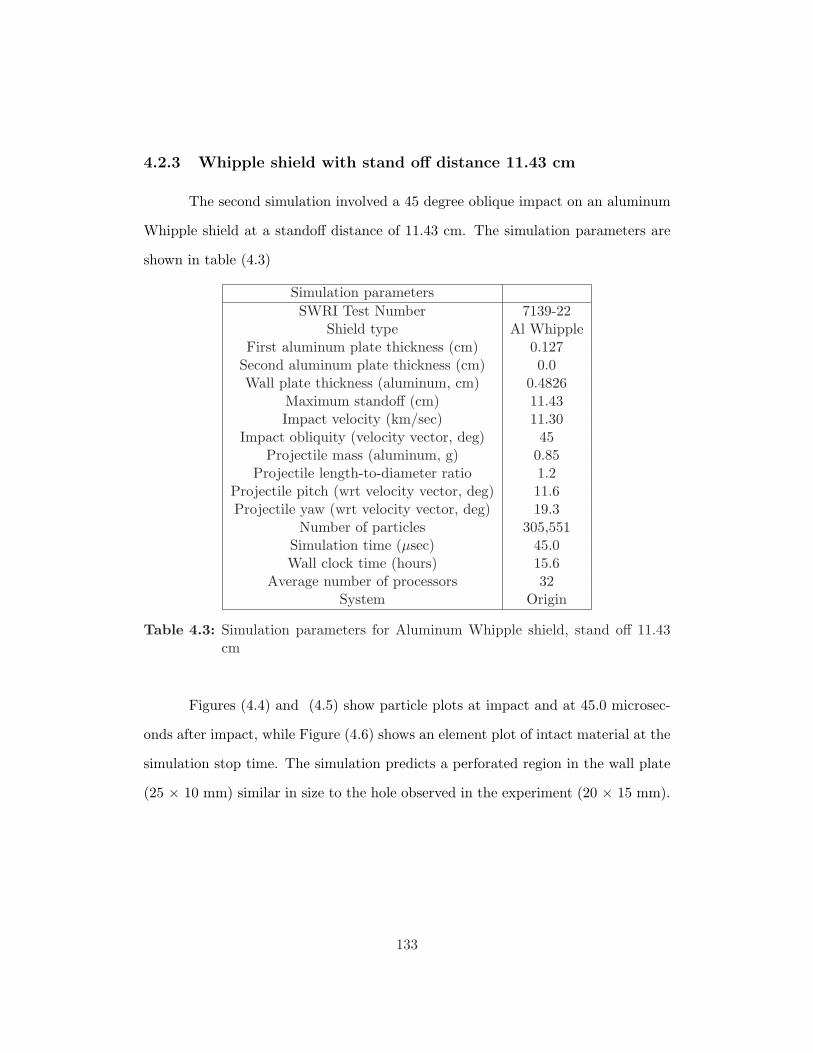
4.2.3 Whipple shield with stand off distance 11.43 cm
The second simulation involved a 45 degree oblique impact on an aluminum
Whipple shield at a standoff distance of 11.43 cm. The simulation parameters are
shown in table (4.3)
Simulation parametersSWRI Test Number 7139-22
Shield type Al WhippleFirst aluminum plate thickness (cm) 0.127
Second aluminum plate thickness (cm) 0.0Wall plate thickness (aluminum, cm) 0.4826
Maximum standoff (cm) 11.43Impact velocity (km/sec) 11.30
Impact obliquity (velocity vector, deg) 45Projectile mass (aluminum, g) 0.85
Projectile length-to-diameter ratio 1.2Projectile pitch (wrt velocity vector, deg) 11.6Projectile yaw (wrt velocity vector, deg) 19.3
Number of particles 305,551Simulation time (µsec) 45.0Wall clock time (hours) 15.6
Average number of processors 32System Origin
Table 4.3: Simulation parameters for Aluminum Whipple shield, stand off 11.43cm
Figures (4.4) and (4.5) show particle plots at impact and at 45.0 microsec-
onds after impact, while Figure (4.6) shows an element plot of intact material at the
simulation stop time. The simulation predicts a perforated region in the wall plate
(25 × 10 mm) similar in size to the hole observed in the experiment (20 × 15 mm).
133

Figure 4.4: Whipple shield impact simulation: 11.43cm stand off distance, initialconfiguration, particle plot
134
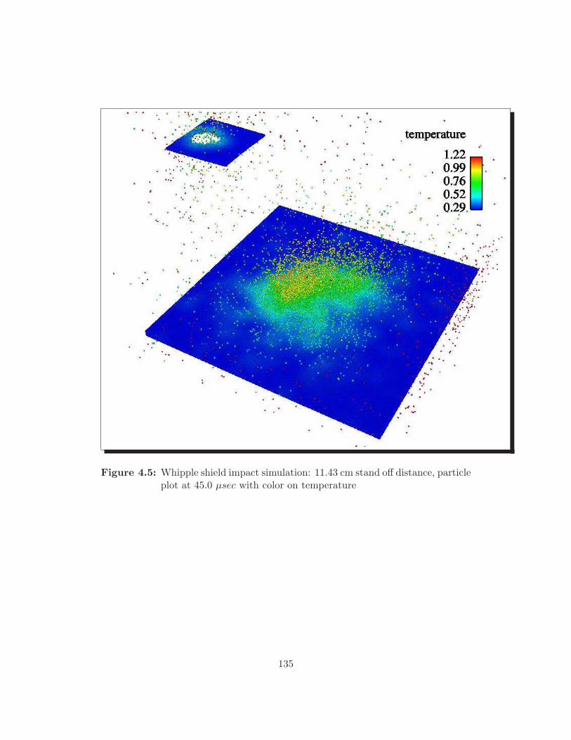
Figure 4.5: Whipple shield impact simulation: 11.43 cm stand off distance, particleplot at 45.0 µsec with color on temperature
135
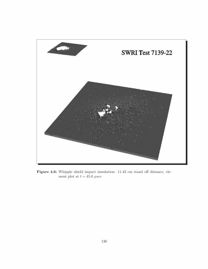
Figure 4.6: Whipple shield impact simulation: 11.43 cm stand off distance, ele-ment plot at t = 45.0 µsec
136

4.2.4 Normal impact on dual plate aluminum shield
The third simulation involved a normal impact on a dual plate aluminum
shield at a standoff distance of 8.636 cm. In this case the axis of the cylindrical
projectile and the velocity vector were significantly misaligned, again calling for a
three dimensional simulation. The simulation parameters are shown in table (4.4).
Simulation parametersSWRI Test Number 7139-03
Shield type Al dual plateFirst aluminum plate thickness (cm) 0.16002
Second aluminum plate thickness (cm) 0.3175Nextel areal density (g/cm2) 0.0Kevlar areal density (g/cm2) 0.0
Wall plate thickness (aluminum, cm) 0.2032Maximum standoff (cm) 8.636Impact velocity (km/sec) 11.16
Impact obliquity (velocity vector, deg) 0Projectile mass (aluminum, g) 1.30
Projectile length-to-diameter ratio 1.84Projectile pitch (wrt velocity vector, deg) 12.6Projectile yaw (wrt velocity vector, deg) 6.9
Number of particles 265,251Simulation time (µsec) 30.7Wall clock time (hours) 15.6
Average number of processors 32System Origin
Table 4.4: Parameters for the example simulations
Figures (4.7) and (4.8) show particle plots at impact and at 30.7 microseconds
after impact, while Figure (4.9) shows an element plot of intact material at the
simulation stop time. The simulation predicts a wall plate hole diameter (55 mm)
somewhat greater than that observed in the experiment (44 mm).
137
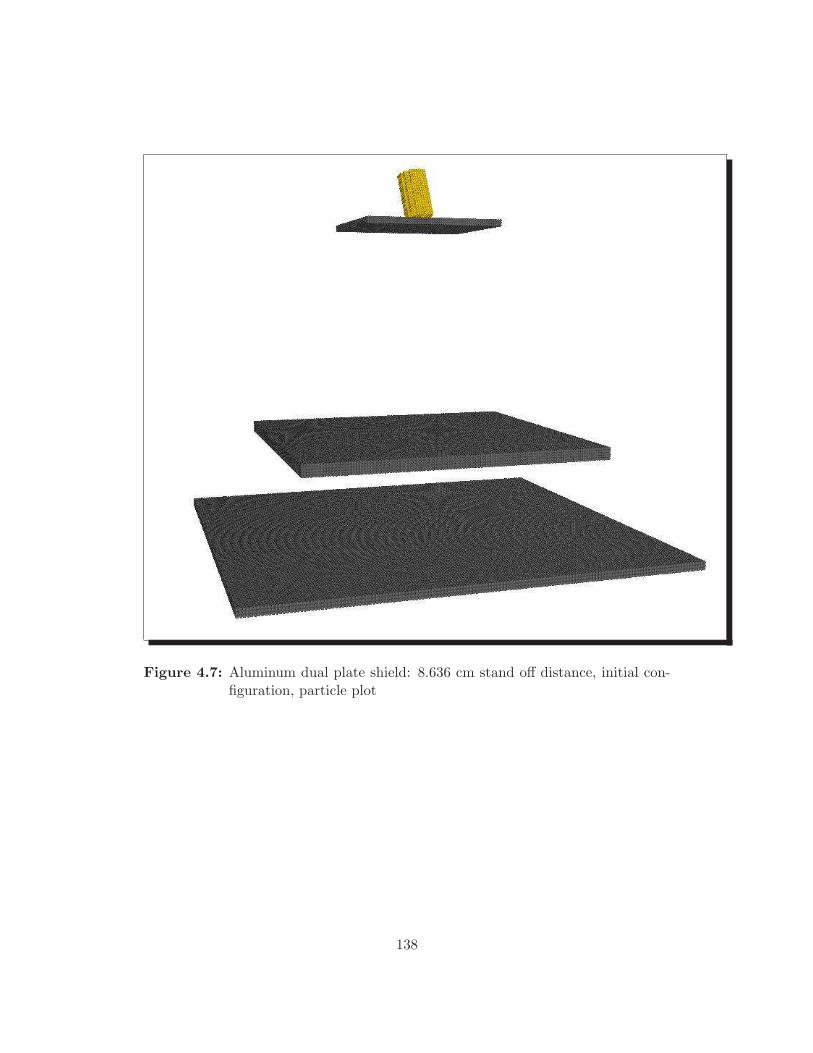
Figure 4.7: Aluminum dual plate shield: 8.636 cm stand off distance, initial con-figuration, particle plot
138

Figure 4.8: Aluminum dual plate shield: 8.636 cm stand off distance,particle plotat 30.7 µsec with color on temperature
139

Figure 4.9: Aluminum dual plate shield: 8.636 cm maximum stand off distance,element plot at 30.7 µsec
140

4.2.5 Multi-layer Aluminum-Nextel-Kevlar shield
The fourth simulation involved a 45 degree oblique impact on a multi-layer
aluminum-Nextel-Kevlar shield at a standoff distance of 7.62 cm. The simulation
parameters are shown in table (4.5).
ParametersSWRI Test Number 7139-24
Shield type Al-compositeFirst aluminum plate thickness (cm) 0.127
Second aluminum plate thickness (cm) 0.0Nextel areal density (g/cm2) 0.4Kevlar areal density (g/cm2) 0.128
Wall plate thickness (aluminum, cm) 0.3175Maximum standoff (cm) 7.62Impact velocity (km/sec) 11.25
Impact obliquity (velocity vector, deg) 45Projectile mass (aluminum, g) 1.07
Projectile length-to-diameter ratio 1.1Projectile pitch (wrt velocity vector, deg) 0Projectile yaw (wrt velocity vector, deg) 0
Number of particles 415,413Simulation time (µsec) 46.2Wall clock time (hours) 109.3
Average number of processors 7.3System Onyx
Table 4.5: Parameters for the example simulations
Figures (4.10) and (4.11) show particle plots at impact and at 46.2 microsec-
onds after impact, while Figure (4.12) shows an element plot of intact material at
the simulation stop time. Consistent with the experimental results, the simulation
predicts bulging but not perforation of the wall plate. It should be noted that
some relevant material properties of Nextel and Kevlar are not well known, and are
currently under study [32]. Although the linear elastic response of many composite
materials has been well characterized, information on thermomechanical equation of
141

state properties and plasticity properties is limited. Although the latter information
is normally of secondary interest in structural design calculations, it is certainly of
major interest in hypervelocity impact applications.
Figure 4.10: Aluminum Nextel Kevlar shield: 7.62 cm maximum stand off dis-
tance, initial configuration, particle plot
142

Figure 4.11: Aluminum Nextel Kevlar shield: 7.62 cm maximum stand off dis-
tance, particle plot at 46.2 µsec with color on temperature
143

Figure 4.12: Aluminum Nextel Kevlar shield: 7.62 cm maximum stand off dis-
tance, element plot at 46.2 µsec
The results just described show in general good agreement of the simulations
with the experimental data. They do suggest a need for higher resolution models,
longer physical simulation times, and better composite material models in future
simulation work.
144
4.3 Projectile shape effect
As noted in the last section, the geometry of projectiles produced by ISC
experiments differs markedly from the solid spherical shape normally used in LGG
tests. Since light gas guns operate in a lower velocity regime, correlating the results
of ISC launcher and LGG tests is complicated by an unknown projectile shape ef-
fect. In an attempt to investigate the significance of this projectile shape effect, the
first three ISC simulations described in the last section were repeated, with mass
equivalent spherical projectiles replacing the actual hollow cylindrical ISC projec-
tiles. Figures (4.13), (4.15), and (4.17) show element plots of the wall plate damage
predictions obtained from simulations using hollow cylindrical ISC projectiles and
mass equivalent spherical projectiles, run in each case to the same simulation stop
time.
145

Figure 4.13: Wall damage for ISC projectile, Whipple shield 7.62cm stand off
Figure 4.14: Wall damage for spherical projectile, Whipple shield 7.62cm standoff
146
Figure 4.15: Wall damage for ISC projectile, Whipple shield 11.43cm stand off
Figure 4.16: Wall damage for spherical projectile, Whipple shield 11.43cm standoff
147

Figure 4.17: Wall damage for ISC projectile, dual plate aluminum shield 8.636cmstand off
Figure 4.18: Wall damage for spherical projectile, dual plate aluminum shield8.636cm stand off
148

The results suggest that ISC projectiles are more damaging than mass equiv-
alent spheres, although the magnitude of the difference is difficult to quantify. In
the first and third cases the projectile mass exceeds significantly the ballistic limit
mass, and in all cases higher resolution models of the impact problems are needed
in order to draw more definitive conclusions. However it should be noted that since
the ISC projectiles:
(1) are hollow
(2) exhibit pitch and yaw with respect to their velocity vector, and
(3) involve rather low length-to-diameter ratios,
one might expect to observe a modest projectile shape effect. Considering the com-
plex nature of these highly oblique hypervelocity impact problems, it appears that
more experimental and computational work is needed to address the question of
projectile shape effects.
4.4 Parallel speedup
Three dimensional impact simulations require large memory and CPU time
allocations. Previous work on orbital debris shielding design [21] has reported wall
clock times as high as eighteen days for single processor simulations of three di-
mensional problems. Such turnaround times effectively preclude the use computer
simulation in many engineering design projects. Parallel processing offers an oppor-
tunity to greatly reduce turnaround time and make three dimensional simulation a
more practical design tool.
The code used in the present work [16] was written for parallel execution
on Onyx and Origin systems, using loop level compiler directives based on the
149
OpenMP standard. Alternative parallel implementations based on MPI constructs
are in general more portable and presumably more efficient, although more difficult
to implement. It should be emphasized that a high degree of parallelism must be
present in the basic numerical algorithm in order to achieve good speedup under
any coding scheme.
To evaluate parallel performance of the numerical algorithm and the code
implementation used here, speedup tests were run on Origin systems with up to 128
processors. The test problems were large (300,000 - 500,000 particles), to insure
that a meaningful load was maintained on each CPU as the processor allocation
increased. Figure (4.19) shows the absolute speedup measured for a 500,000 particle
test problem, based on the wall clock time required for ten time steps at various
CPU allocations.
20 40 60 80 100 120number of processors
20
40
60
80
100
120
speedup
System: Origin 2000
Implementation: OpenMP
Problem size: 514,046 particles
Figure 4.19: Absolute speedup for a 1GB size problem on Origin2000
The dotted line shows the maximum theoretical speedup, while the data
points indicate the test results. At a CPU allocation of 64, the measured speedup
150

is approximately two thirds of the theoretical maximum, indicating good parallel
performance. At the maximum CPU allocation of 128, the efficiency drops to fifty
percent. However the latter data point represents a factor of 64 reduction in wall
clock time, indicating that a simulation which runs for over two months on one CPU
can be run in one day on 128 processors.
Massively parallel systems are characterized by distributed memory archi-
tectures, complicating somewhat the practical interpretation of speedup test data.
The Origin system discussed here is composed of a collection of compute nodes,
each of which consists of two processors and 512 MB of RAM. An individual user
is allocated a discrete number of nodes for each particular job, that is allocations
consisting of arbitrary combinations of processors and RAM are not permitted. As
a result, a particular job which requires 1 GB of RAM will be allocated a mini-
mum of four processors, and the meaningful speedup curve for such a problem is
one measured relative to a CPU allocation of four. Figure (4.20) shows the results
of a relative speedup test run on an Origin system, for ten time steps of a 300,000
particle test problem, using the code discussed in the present work. The solid line
represents the maximum theoretical relative speedup, while the data points show
the test results. Again the data show good speedup for processor allocations as high
as 64.
High performance parallel computer systems are not yet commonplace in
engineering design work. However the preceding results demonstrate that the nu-
merical method used here can effectively exploit such resources, an important con-
sideration as low cost, high performance parallel hardware becomes more widely
available.
151

10 20 30 40 50 60 70number of cpus
2.5
5
7.5
10
12.5
15
17.5Speedup relative to 4 cpus
Figure 4.20: Relative speedup for a 1GB size problem on Origin2000
4.5 Conclusion
A systematic test of the use of parallel computation and a hybrid particle-
element algorithm to simulate a range of three dimensional orbital debris impact
experiments has been performed. The numerical method appears to offer certain
advantages in addressing the three dimensional, multi-plate shield design problem.
Additional work is needed to investigate model resolution, simulation time, projectile
shape, and material property effects (including for example the use of the SESAME
equation of state models). However developments to date suggest that massively
parallel computation using some type of mixed particle-continuum scheme offers
excellent opportunities for significant advances in simulation-based debris shield
design.
152

Chapter 5
Summary and Future work
In this chapter a summary of the work done and a discussion of future work
is presented. Note that conclusions were presented at the end of each chapter.
Most of existing particle methods use spherical particles, the use of which to
model structures such as thin plates results in an exorbitant number of particles.
The present work has developed a general hybrid particle finite element method to
model hypervelocity impact. The model development uses thermo-mechanically in-
teracting ellipsoidal particles, resulting in reduced computer resource requirements
for hypervelocity impact simulations. Foreseeing the requirement to model the ro-
tational dynamics of ellipsoidal particles, an efficient, singularity free rigid body ro-
tational dynamics model was developed in chapter (2). Rotation was parameterized
using four Euler parameters. The use of these parameters simplified the kinematic
description, with a moderate increase in complexity of the dynamics. Previous work
using Euler parameters for parameterizing rotation uses Lagrange multipliers, an
additional momentum variable, or adds the constraint as an auxiliary differential
equation. In contrast the model developed in here uses three angular momenta and
four Euler parameters to describe the rotational dynamics. The model does not
153

make use of any unknown Lagrange multiplier, to implement the Euler parameter
constraint.
Although the use of both particles and finite elements results in increased
computational cost, it provides the ability to model the disintegration of a solid into
comminuted fluid, with ease. In addition, the use of particles simplifies problems
involved in modeling contact-impact with pure finite elements. A classical weighted
residual solution technique is rejected in favor of a system dynamics development.
The benefits of such an approach are seen in the results of numerical simulations,
presented in chapters (3) and (4). It is suggested that future work should intro-
duce more complex material models, such as composites. Future shield design will
increasingly rely on the use of such materials, due to their high strength to weight
ratio.
154

Bibliography
[1] S.W. Attaway, M.W. Heinstein, J.W. Swegle. Coupling of smooth particle hy-
drodynamics with the finite element method. Nuclear Engineering and Design,
150:199–205, 1994.
[2] S.G. Bardenhagen, J.U. Brackbill, Deborah Sulsky. The material-point method
for granular materials. Computer methods in applied mechanics and engineer-
ing, 187:529–541, 2000.
[3] Haim Baruh. Analytical Dynamics. WCB/McGraw Hill, 1999.
[4] Klaus-Jurgen Bathe. Finite element Procedures. Prentice Hall, Englewood
Cliffs, New Jersey, 1996.
[5] Eric E. Becker, Graham F. Carey, J.Tinsley Oden. Finite elements: An intro-
duction. Prentice Hall, Inc, Englewood Cliffs, New Jersey, 1983.
[6] T. Belytschko, Y. Krongauz, D. Organ, M.Fleming, P.Krysl. Meshless methods:
An overview and recent developments. Computer methods in applied mechanics
and engineering, 139:3–47, 1996.
[7] David J. Benson. Computational methods in Lagrangian and Eulerian hy-
drocodes. Computer methods in Applied mechanics and Engineering, 99:235–
394, 1992.
155

[8] J.U. Brackbill, H.M. Ruppel. FLIP: a method for adaptivley zoned, particle
in cell calcualtions of fluid flows in two dimensions. Journal of Computational
Physics, 65:314–343, 1986.
[9] D. Burgess, D. Sulsky, J.U. Brackbill. Mass matrix formulation of the FLIP
particle-in-cell method. Journal of Computational Physics, 103:1–15, 1992.
[10] C. O. Chang, C.S. Chou. Design of a viscous ring nutation damper for a freely
precessing body. Journal of Guidance, Control and Dynamics, 14:1136–1144,
1991.
[11] Eric L. Christiansen. Design and performance equations for advanced meteoroid
and debris shields. International Journal of Impact Engineering, 14:145–156,
1993.
[12] R.H. Cole. Underwater Explosions. Dover Publications, New York, 1948.
[13] Burton G. Cour-Palais. A multi-shock concept for spacecraft shielding. Inter-
national Journal of Impact Engineering, 10:135–146, 1990.
[14] C.T. Dyka, R.P. Ingel. An approach for tension instability in smoothed particle
hydrodynamics. Computers and Structures, 57:573–580, 1995.
[15] E. P. Fahrenthold, B.A. Horban. Thermodynamics of continuum damage and
fragmentation models for hypervelocity impact. International Journal of Impact
Engineering, 20:241–252, 1997.
[16] E.P. Fahrenthold. User’s guide for EXOS. Technical report, University of Texas,
Austin, 1999.
[17] E.P. Fahrenthold, J.C. Koo. Hamiltonian particle hydrodynamics. Computer
methods in Applied Mechanics and Engineering, 146:43–52, 1997.
156

[18] E.P. Fahrenthold, J.C. Koo. Hybrid particle-element bond graphs for impact
dynamics simulation. Journal of Dynamic Systems, Measurement, and Control,
122:306–313, 2000.
[19] Eric Fahrenthold, Blaise Horban. An improved particle-element method for
hypervelocity impact simulation. International Journal of Impact Engineering,
26:169–178, 2001.
[20] Eric P. Fahrenthold, Blaise A. Horban. A hybrid particle-finite element method
for hypervelocity impact simulation. International Journal of Impact Engineer-
ing, 23:237–248, 1999.
[21] Moreno Faraud, Roberto Destefanis, David Palmieri, Mario Marchetti. SPH
simulations of debris impacts using two different computer codes. International
Journal of Impact Engineering, 23:249–260, 1999.
[22] Michael S. Fulbright, Willy Benz, Melvyn B. Davies. A method of smoothed
particle hydrodynamics using spheroidal kernels. The Astrophysical Journal,
440:254–262, 1995.
[23] J.H Ginsberg. Advanced Engineering Dynamics. Harper & Row, 1988.
[24] Herbert Goldstein. Classical Mechanics. Addison-Wesley Publishing Company,
Inc, 1965.
[25] Donald T. Greenwood. Principles of Dynamics. Prentice Hall, Inc., Englewood
Cliffs, New Jersey 07632, 1988.
[26] D.J. Grosch. Inhibited shaped charge launcher testing of spacecraft shield de-
signs. Technical report, Southwest Research Institute, San Antonio, TX, April
1997.
157
[27] D.J. Grosch. Inhibited shaped charge launcher testing of spacecraft shield
designs. Technical report, Southwest Research Institute, San Antonio, TX,
November 1996.
[28] Francis H. Harlow. The particle-in-cell method for fluid dynamics. Methods in
Computational Physics, 3:319–343, 1964.
[29] C.J. Hayhurst, I.H. Livingstone, R.A. Clegg, G.E. Fairlie, S.H. Hier-
maier,M. Lambert. Numerical simulation of hypervelocity impacts on aluminum
and Nextel/Kevlar whipple shields. In Proceedings of the Hypervelocity Shield-
ing Workshop, pages 61–72, Galvestion, TX, USA, 1998.
[30] E.S. Hertel. Sandia report sand92-1879. Technical report, Sandia National
Labs, Sep 1992.
[31] D.L. Hicks, L.M. Liebrock. SPH hydrocodes can be stablized with shape-lifting.
Computers and Mathematics with Applications, 38:1–16, 1999.
[32] S. Hiermaier, W. Riedel, C.J. Hayhurst, R.A. Clegg, C.M. Wentzel. Advanced
material models for hypervelocity impact simulations. Technical report, EMI-
Report Number E 43/99, Freiburg, Germany, 1999.
[33] R.W. Hockney, J.W. Eastwood. Computer Simulation using particles. McGraw
Hill Inc.,, New York, 1981.
[34] T.J.R. Hughes. The Finite Element method–Linear Static and Dynamic Finite
Element Analysis. Dover Publishers, New York, 2000.
[35] Gordon Johnson. Linking of Lagrangian particle methods to standard finite
element methods for high velocity computations. Nuclear Engineering and
Design, 150:265–274, 1994.
158

[36] Gordon R. Johnson. Artificial viscosity effects for SPH impact computations.
International Journal of Impact Engineering, 18:477–488, 1996.
[37] Gordon R. Johnson, Stephen R. Beissel. Normalized smoothing functions for
sph impact computations. International Journal of Numerical methods in En-
gineering, 39:2725–2741, 1996.
[38] Nicholas L. Johnson, Darren S. Mcknight. Artificial Space debris. Krieger
Publishing Company, Malabar, Florida, 1991.
[39] Charles E. Anderson Jr. An overview of the theory of hydrocodes. In Hyper-
velocity Impact, Proceedings of the 1986 Symposium, 1986.
[40] Harold S. Morton Jr. Hamiltonian and Lagrangian formulations of rigid body
rotational dynamics based on euler parameters. The Journal of Astronautical
Sciences, 41(4):561–591, 1993.
[41] S.L. Lee. Reference book for composites technology. Technomic Publishing,
Lancaster, Pennsylvania, 1989.
[42] J. Lemaitre. Local approach of fracture. Engineering Fracture mechanics,
25:523–537, 1986.
[43] L.D. Libersky, P.W. Randles, T.C. Carney, D.L. Dickinson. Recent improve-
ments in SPH modelling of hypervelocity impact. International Journal of
Impact Engineering, 20:525–532, 1997.
[44] Wing Kam Liu, Su Hao, Ted Belytschko, Shofan Li, Chin Tang Chang. Mul-
tiscale methods. International Journal of Numerical methods in Engineering,
47:1343–1361, 2000.
159

[45] W.K. Liu, Y.Chen, S. Jun, J.S. Chen, T. Belytschko, C. Pan, R.A. Uras, C.T.
Chang. Overview and applications of the Reproducing kernel particle methods.
Archives of Computational Methods in Engineering: State of the art reviews,
3:3–80, 1996.
[46] Leonard Meirovitch. Elements of Vibration Analysis. McGraw-Hill Book Com-
pany, 1986.
[47] J.J. Monoghan. Particle methods for hydrodynamics. Computer Physics Re-
ports, 3:71–124, 1985.
[48] J.J. Monoghan. On the problem of penetration in particle methods. Journal
of Computational Physics, 82:1–15, 1989.
[49] J.J. Monoghan. SPH without tensile instability. Journal of Computational
Physics, 159:290–311, 2000.
[50] P.E. Nikravesh, I.S. Chung. Application of Euler parametes to the dynamic
analysis of three dimensional constrained mechanical systems. Journal of Me-
chanical Design, 104:785–791, October 1982.
[51] P.E. Nikravesh, O.K. Kwon, R.A. Wehage. Euler parameters in computational
kinematics and dynamics. part 2. Journal of Mechanisms, Transmissions and
Automation Design, 107:366–369, September 1985.
[52] P.E. Nikravesh, R.A. Wehage, O.K. Kwon. Euler parameters in computational
kinematics and dynamics. part 1. Journal of Mechanisms, Transmissions and
Automation Design, 107:358–365, September 1985.
[53] Praviz E. Nikravesh. Computer aided analysis of Mechanical Systems. Prentice
Hall, 1988.
160

[54] Martin Nitschke, Ernst Heinrich Knickmeyer. Rotation parameters- a survey
of techniques. Journal of Surveying Engineering, 126(3):83–105, August 2000.
[55] W.F. Noh. Errors for calculations of strong shocks using an artificial viscosity
and an artificial heat flux. Journal of Computational Physics, 72:78–120, 1978.
[56] Committee on Space debris, Aeronautics and Space Engineering board, Comis-
sion of Engineering, Technical systems, National Research Council. Orbital
debris, A technical assessment. National Academy Press, Washington, D.C.,
1995.
[57] J. Michael Owen, Jens V. Villumsen, Paul R. Shapiro, Hugo Martel. Adaptive
smoothed particle hydrodynamics: methodology II. The Astrophysical Journal
Supplement Series, 116:155–209, June 1998.
[58] Anatoly N. Parshikov, Stanislav A. Medin, Igor I. Laukashenko, Valery A.
Milekhin. Improvements of SPH method by means of interparticle contact
algorithm and analysis of perforation tests at moderate projectile velocities.
International Journal of Impact Engineering, 24:779–796, 2000.
[59] Piekutowski, A.J. Formation and description of debris clouds produced by
hypervelocity impact. NASA contractor report 4707, 1996
[60] P.W. Randles, L.D. Libersky. Smoothed particle hydrodynamics: Some recent
improvements and applications. Computer methods in Applied mechanics and
Engineering, 139:375–408, 1996.
[61] P.W. Randles, L.D. Libersky. Normalized SPH with stress points. International
Journal of Impact Engineering, 48:1445–1462, 2000.
[62] D. C. Rapaport. Molecular dynamics simulation using quaternions. Journal of
Computational Physics, 60:306–314, 1985.
161
[63] Dietrich Rex. Will space run out of space? the orbital debris problem and its
mitigation. Space Policy, 14:95–105, 1998.
[64] Paul R. Shapiro, Hugo Martel, Jens V. Villumsen,J. Michael Owen. Adaptive
smoothed particle hydrodynamics with application to cosmology: methodology
I. The Astrophysical Journal Supplement Series, 103:269–330, April 1996.
[65] M.D Shuster. A survey of attitude representations. Journal of Astronautical
Sciences, 41:531–543, 1993.
[66] J.C. Simo, K.K. Wong. Unconditionally stable algorithms for rigid body dy-
namics that exactly preserve energy and momentum. International Journal of
Numerical methods in Engineering, 31:19–52, 1991.
[67] Kerry W. Spring. Euler parameters and the use of quaternion algebra in the
manipulation of finite rotations: A review. Mechanism and Machine Theory,
21(5):365–373, 1991.
[68] D.J. Steinberg. Equation of state and strength properties of selected materials.
Technical report, Lawrence Livermore National Laboratory,UCRL-MA-106439,
1996.
[69] William Tyrrell Thompson. Introduction to Space Dynamics. John Wiley &
Sons, Inc, 1961.
[70] Srinivas R. Vadali. On the Euler parameter constraint. The Journal of Astro-
nautical Sciences, 36(3):259–265, 1988.
[71] R. Vignjevic, J. Campbell. A penalty approach for contact in smooth particle
hydrodynamics. ijie, 23:945–956, 1999.
162
[72] R. Vignjevic, J. Campbell, L.Libersky. A treatment of zero energy modes in
smooth particle hydrodynamics. Computer methods in Applied mechanics and
Engineering, 184:67–85, 2000.
[73] F.L. Whipple. Meteorites and space travel. The Astronomical Journal, 52:131,
1947.
[74] Mark L. Wilkins. Computer Simulation of Dynamics Phenomena. Springer,
1999.
[75] Jerome D. Yatteau, Gunnar W. Recht, Karl T. Edquist. Transverse loading
and response of long road penetrators during high velocity plate perforation.
International Journal of Impact Engineering, 23:967–980, 1999.
[76] Jonas A. Zukas. High velocity impact dynamics, chapter 9, pages 593–709. John
Wiley and Sons, Inc., 1990.
163

Vita
Ravishankar Ajjanagadde Shivarama is the eldest son of Sarojini and A.V.
Shivarama was born on June 22, 1972. He grew up in the city of Bangalore, the cap-
ital of the southern state Karnataka, India. After completing his schooling at Vijaya
High school and St. Joseph’s college, Bangalore, he entered Bangalore University
from where he graduated with a Bachelor of Engineering in Mechanical Engineering
in 1994. In the same year he joined the Mechanical Engineering Department at the
Indian Institute of Science (IISc), Bangalore. At IISc, he was a research scholar and
worked in the area of robot dynamics and control. In 1997 he received a Master of
Science in Engineering degree for his research on “Possible chaos in robot control
equations ”. From January 1997 to July 1997, he worked as a software engineer at
Altair Software India Limited. In the fall of 1997, he joined the doctoral program at
the University of Texas at Austin to continue his studies in Mechanical Engineering.
He received the Bruton fellowship (2000-2001) and Alfred and Nellie King fellowship
(2001-2002) for his scholastic accomplishments. After completing his Ph.D studies,
Ravishankar will join the servo-mechanics group at Seagate Technology Inc.
Permanent Address: #256, AECS Layout I stage, 4th main cross,
Geddalahalli, Bangalore-560094
This dissertation was typeset with LATEX2ε1 by the author.
1LATEX2ε is an extension of LATEX. LATEX is a collection of macros for TEX. TEX is a trademarkof the American Mathematical Society.
164


