35
Copyright © Cengage Learning. All rights reserved. 12 Further Applications of the Derivative
| Date post: | 19-Dec-2015 |
| Category: |
Documents |
| View: | 215 times |
| Download: | 0 times |

Copyright © Cengage Learning. All rights reserved.
12 Further Applicationsof the Derivative

Copyright © Cengage Learning. All rights reserved.
12.3 Higher Order Derivatives: Acceleration and Concavity

33
Higher Order Derivatives: Acceleration and Concavity
The second derivative is simply the derivative of the
derivative function.

44
Acceleration

55
Acceleration
Recall that if s(t) represents the position of a car at time t, then its velocity is given by the derivative: v(t) = s(t). But one rarely drives a car at a constant speed; the velocity itself is changing.
The rate at which the velocity is changing is the acceleration. Because the derivative measures the rate of change, acceleration is the derivative of velocity: a(t) = v(t).
Because v is the derivative of s, we can express the acceleration in terms of s:
a(t) = v(t) = (s)(t) = s(t)

66
Acceleration
That is, a is the derivative of the derivative of s, in other words, the second derivative of s, which we write as s. (In this context you will often hear the derivative s referred toas the first derivative.)
Second Derivative, Acceleration
If a function f has a derivative that is in turn differentiable, then its second derivative is the derivative of the derivative of f, written as f .
If f (a) exists, we say that f is twice differentiable at x = a.

77
Acceleration
Quick Example
If f (x) = x3 – x, then f (x) = 3x2 – 1, so f (x) = 6x and f (–2) = –12.
The acceleration of a moving object is the derivative of its velocity—that is, the second derivative of the position function.
Quick ExampleIf t is time in hours and the position of a car at time t is s(t) = t3 + 2t2 miles, then the car’s velocity is v(t) = s(t) = 3t2 + 4t miles per hour and its acceleration is a(t) = s(t) = v(t) = 6t + 4 miles per hour per hour.

88
Differential Notation for the Second Derivative

99
Differential Notation for the Second Derivative
We have written the second derivative of f (x) as f (x).
We could also use differential notation:
This notation comes from writing the second derivative as
the derivative of the derivative in differential notation:

1010
Differential Notation for the Second Derivative
Similarly, if y = f (x), we write f (x) as
For example, if y = x3, then
An important example of acceleration is the acceleration due to gravity.

1111
Example 1 – Acceleration Due to Gravity
According to the laws of physics, the height of an object near the surface of the earth falling in a vacuum from an initial rest position 100 feet above the ground under theinfluence of gravity is approximately
s(t) = 100 – 16t2 feet
in t seconds. Find its acceleration.
Solution:
The velocity of the object is
v(t) = s(t) = –32t ft/s.

1212
Example 1 – Solution
The reason for the negative sign is that the height of the object is decreasing with time, so its velocity is negative.
Hence, the acceleration is
a(t) = s(t) = –32 ft/s2.
(We write ft/s2 as an abbreviation for feet/second/second—that is, feet per second per second. It is often read “feet per second squared.”)
Thus, the downward velocity is increasing by 32 ft/s every second.
cont’d

1313
Example 1 – Solution
We say that 32 ft/s2 is the acceleration due to gravity.
If we ignore air resistance, all falling bodies near the surface of the earth, no matter what their weight, will fall with this acceleration.
cont’d

1414
Geometric Interpretation of Second Derivative: Concavity

1515
Geometric Interpretation of Second Derivative: Concavity
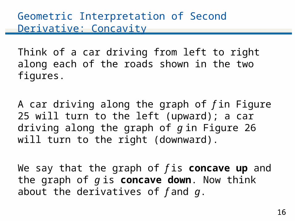
The first derivative of f tells us where the graph of f is rising [where f (x) > 0] and where it is falling [where f (x) < 0]. The second derivative tells in what direction the graph of f curves or bends.
Consider the graphs in Figures 25 and 26.
Figure 25 Figure 26
1616
Geometric Interpretation of Second Derivative: Concavity
Think of a car driving from left to right along each of the roads shown in the two figures.
A car driving along the graph of f in Figure 25 will turn to the left (upward); a car driving along the graph of g in Figure 26 will turn to the right (downward).
We say that the graph of f is concave up and the graph of g is concave down. Now think about the derivatives of f and g.

1717
Geometric Interpretation of Second Derivative: Concavity
The derivative f (x) starts small but increases as the graph gets steeper. Because f (x) is increasing, its derivative f (x) must be positive.
On the other hand, g(x) decreases as we go to the right. Because g(x) is decreasing, its derivative g(x) must be negative.
1818
Geometric Interpretation of Second Derivative: Concavity
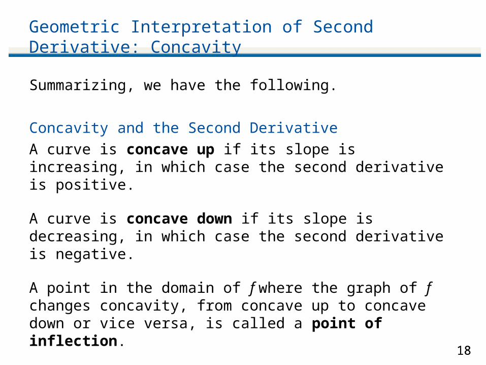
Summarizing, we have the following.
Concavity and the Second Derivative
A curve is concave up if its slope is increasing, in which case the second derivative is positive.
A curve is concave down if its slope is decreasing, in which case the second derivative is negative.
A point in the domain of f where the graph of f changes concavity, from concave up to concave down or vice versa, is called a point of inflection.

1919
Geometric Interpretation of Second Derivative: Concavity
At a point of inflection, the second derivative is either zero
or undefined.
Locating Points of Inflection
To locate possible points of inflection, list points where
f (x) = 0 and also points where f (x) is not defined.

2020
Geometric Interpretation of Second Derivative: Concavity
Quick Example
The graph of the function f shown in Figure 27 is concave up when 1 < x < 3, so f (x) > 0 for 1 < x < 3. It is concave down when x < 1 and x > 3, so f (x) < 0 when x < 1 and x > 3. It has points of inflection at x = 1 and x = 3.
Figure 27

2121
Example 3 – Inflation
Figure 29 shows the value of the U.S. Consumer Price Index (CPI) from January 2007 through June 2008.
Figure 29

2222
Example 3 – Inflation
The approximating curve shown on the figure is given by
I(t) = 0.0075t3 – 0.2t2 + 2.2t + 200 (1 ≤ t ≤ 19)
where t is time in months (t = 1 represents January 2007). When the CPI is increasing, the U.S. economy is experiencing inflation. In terms of the model, this means that the derivative is positive: I(t) > 0. Notice that I(t) > 0 for the entire period shown (the graph is sloping upward), so the U.S. economy experienced inflation for 1 ≤ t ≤ 19.
cont’d

2323
Example 3 – Inflation
We could measure inflation by the first derivative I(t) of the CPI, but we traditionally measure it as a ratio:
expressed as a percentage per unit time (per month in this case).
a. Use the model to estimate the inflation rate in January
2008.
b. Was inflation slowing or speeding up in January 2008?
c. When was inflation slowing? When was inflation speeding up? When was inflation slowest?
cont’d
Relative rate of change of the CPI

2424
Example 3(a) – Solution
We need to compute I(t) :I(t) = 0.0225t2 – 0.4t + 2.2
Thus, the inflation rate in January 2008 was given by
or 0.38% per month.

2525
Example 3(b) – Solution
We say that inflation is “slowing” when the CPI is decelerating (I(t) < 0; the index rises at a slower rate).
Similarly, inflation is “speeding up” when the CPI isaccelerating (I(t) > 0; the index rises at a faster rate).
From the formula for I(t), the second derivative is
I(t) = 0.045t – 0.4
I(13) = 0.045(13) – 0.4 = 0.185.
Because this quantity is positive, we conclude that inflation was speeding up in January 2008.
cont’d

2626
Example 3(c) – Solution
When inflation is slowing, I(t) is negative, so the graph of the CPI is concave down. When inflation is speeding up, it is concave up. At the point at which it switches, there is point of inflection (Figure 30).
cont’d
Figure 30

2727
The point of inflection occurs when I(t) = 0; that is,
0.045t – 0.4 = 0
Thus, inflation was slowing when t < 8.9 (that is, until the end of August), and speeding up when t > 8.9 (after that time).
Inflation was slowest at the point when it stopped slowing down and began to speed up, t ≈ 8.9; notice that the graph has the least slope at that point.
Example 3(c) – Solution cont’d

2828
The Second Derivative Test for Relative Extrema

2929
The Second Derivative Test for Relative Extrema
The second derivative often gives us a way of knowing whether or not a stationary point is a relative extremum.
Figure 33 shows a graph with two stationary points: a relative maximum at x = a and a relative minimum at x = b.
Figure 33

3030
The Second Derivative Test for Relative Extrema
Notice that the curve is concave down at the relative maximum (x = a), so that f (a) < 0, and concave up at the relative minimum (x = b), so that f (b) > 0.
Second Derivative Test for Relative Extrema
Suppose that the function f has a stationary point at x = c, and that f (c) exists.
Determine the sign of f (c).
1. If f (c) > 0 then f has a relative minimum at x = c.
2. If f (c) < 0 then f has a relative maximum at x = c.

3131
The Second Derivative Test for Relative Extrema
If f (c) = 0 then the test is inconclusive. You have to use
the first derivative test to determine whether or not f has a
relative extremum at x = c.
Quick Example
f (x) = x2 – 2x has f (x) = 2x – 2 and hence a stationary point
at x = 1. f (x) = 2, and so f (1) = 2, which is positive, so
f has a relative minimum at x = 1.

3232
Higher Order Derivatives

3333
Higher Order Derivatives
There is no reason to stop at the second derivative; we could once again take the derivative of the second derivative to obtain the third derivative, f , and we could take the derivative once again to obtain the fourth derivative, written f
(4), and then continue to obtain f (5), f
(6), and so on (assuming we get a differentiable function at each stage).
Higher Order Derivatives
We define

3434
Higher Order Derivatives
and so on, assuming all these derivatives exist.
Different Notations

3535
Higher Order Derivatives
Quick Example
If f (x) = x3 – x, then f (x) = 3x2 – 1, f (x) = 6x, f (x) = 6,
f (4)(x) = f
(5)(x) = ··· = 0.


