22
Copyright © Cengage Learning. All rights reserved. 14.3 Partial Derivatives
| Date post: | 02-Jan-2016 |
| Category: |
Documents |
| Upload: | mariah-foster |
| View: | 223 times |
| Download: | 4 times |

Copyright © Cengage Learning. All rights reserved.
14.3 Partial Derivatives
22
Partial Derivatives
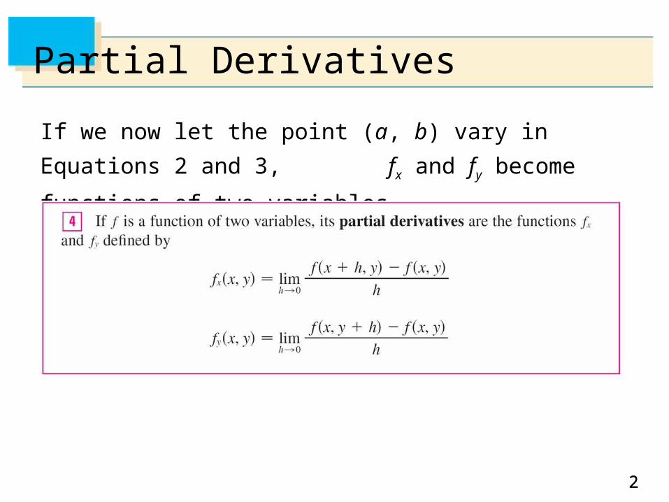
If we now let the point (a, b) vary in Equations 2 and 3,
fx and fy become functions of two variables.

33
Partial Derivatives
There are many alternative notations for partial derivatives.
For instance, instead of fx we can write f1 or D1f (to indicate differentiation with respect to the first variable) or ∂f / ∂x.
But here ∂f / ∂x can’t be interpreted as a ratio of differentials.
44
Partial Derivatives
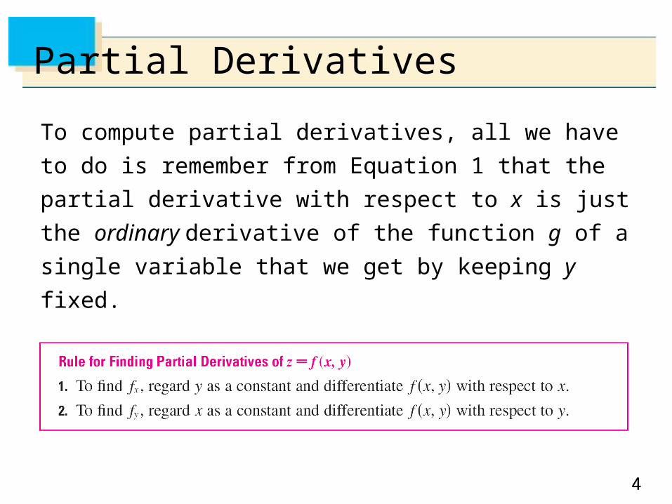
To compute partial derivatives, all we have to do is
remember from Equation 1 that the partial derivative with
respect to x is just the ordinary derivative of the function g
of a single variable that we get by keeping y fixed.
Thus we have the following rule.

55
Example 1
If f (x, y) = x3 + x2y3 – 2y2, find fx(2, 1) and fy(2, 1).
Solution:Holding y constant and differentiating with respect to x, we get
fx(x, y) = 3x2 + 2xy3
and so fx(2, 1) = 3 22 + 2 2 13
Holding x constant and differentiating with respect to y, we get
fy(x, y) = 3x2y2 – 4y
fy(2, 1) = 3 22 12 – 4 1
= 16
= 8

66
Interpretations of Partial Derivatives

77
Example 2
If f (x, y) = 4 – x2 – 2y2, find fx(1, 1) and fy(1, 1) and interpret
these numbers as slopes.
Solution:
We have
fx(x, y) = –2x fy(x, y) = –4y
fx(1, 1) = –2 fy(1, 1) = –4

88
Example 2 – Solution
The graph of f is the paraboloid z = 4 – x2 – 2y2 and the vertical plane y = 1 intersects it in the parabola z = 2 – x2, y = 1. (As in the preceding discussion, we label it C1 in Figure 2.)
The slope of the tangent line to this parabola at the point(1, 1, 1) is fx(1, 1) = –2.
Figure 2
cont’d
99
Example 2 – Solution
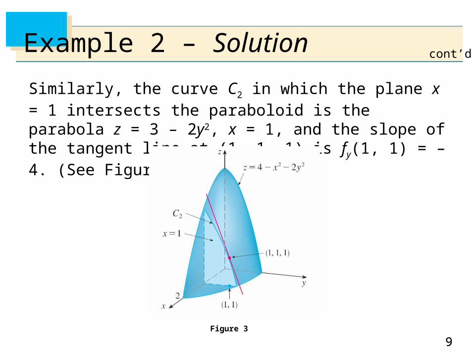
Similarly, the curve C2 in which the plane x = 1 intersects the paraboloid is the parabola z = 3 – 2y2, x = 1, and the slope of the tangent line at (1, 1, 1) is fy(1, 1) = –4. (See Figure 3.)
Figure 3
cont’d

1010
Functions of More Than Two Variables
1111
Functions of More Than Two Variables
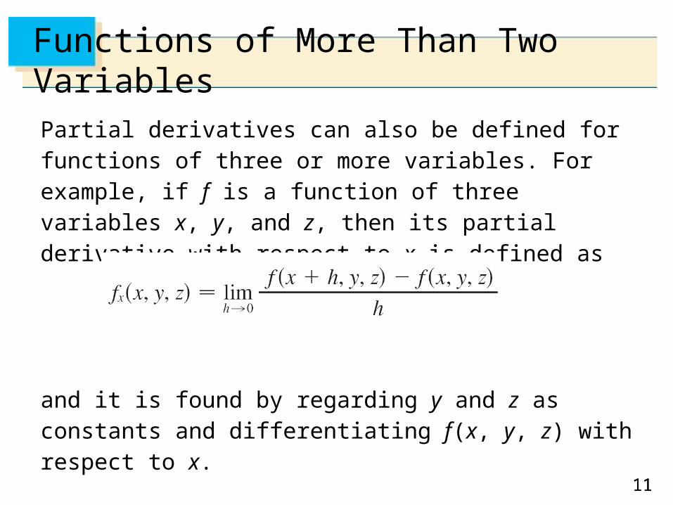
Partial derivatives can also be defined for functions of three or more variables. For example, if f is a function of three variables x, y, and z, then its partial derivative with respect to x is defined as
and it is found by regarding y and z as constants and differentiating f (x, y, z) with respect to x.
1212
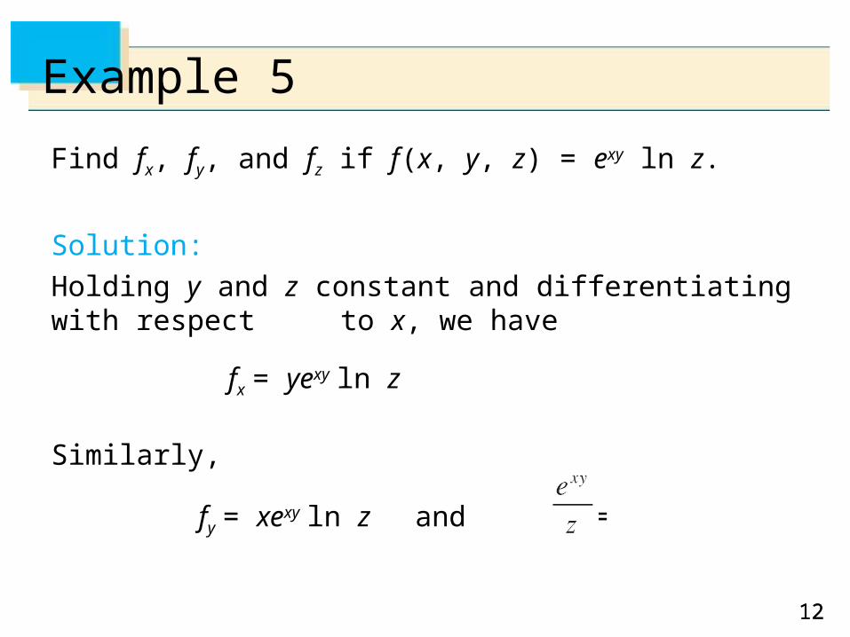
Example 5
Find fx, fy, and fz if f (x, y, z) = exy ln z.
Solution:
Holding y and z constant and differentiating with respect to x, we have
fx = yexy ln z
Similarly,
fy = xexy ln z and fz =
1313
Higher Derivatives

1414
Higher Derivatives
If f is a function of two variables, then its partial derivatives
fx and fy are also functions of two variables, so we can
consider their partial derivatives (fx)x, (fx)y, (fy)x, and (fy)y,
which are called the second partial derivatives of f.
If z = f (x, y), we use the following notation:

1515
Higher Derivatives
Thus the notation fxy (or ∂2f / ∂y ∂x) means that we first
differentiate with respect to x and then with respect to y,
whereas in computing fyx the order is reversed.

1616
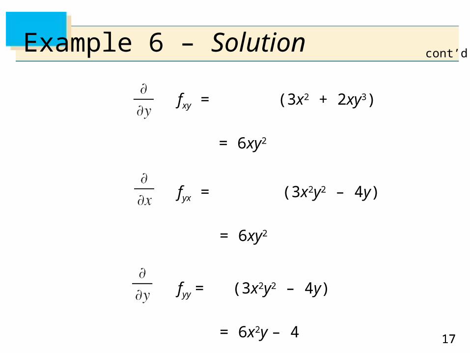
Example 6
Find the second partial derivatives of
f (x, y) = x3 + x2y3 – 2y2
Solution:
In Example 1 we found that
fx(x, y) = 3x2 + 2xy3 fy(x, y) = 3x2y2 – 4y
Therefore
fxx = (3x2 + 2xy3)
= 6x + 2y3
1717
Example 6 – Solution
fxy = (3x2 + 2xy3)
= 6xy2
fyx = (3x2y2 – 4y)
= 6xy2
fyy = (3x2y2 – 4y)
= 6x2y – 4
cont’d

1818
Higher Derivatives
Notice that fxy = fyx in Example 6. This is not just a coincidence.
It turns out that the mixed partial derivatives fxy and fyx are equal for most functions that one meets in practice.
The following theorem, which was discovered by the French mathematician Alexis Clairaut (1713–1765), gives conditions under which we can assert that fxy = fyx.

1919
Higher Derivatives
Partial derivatives of order 3 or higher can also be defined.
For instance,
and using Clairaut’s Theorem it can be shown that
fxyy = fyxy = fyyx if these functions are continuous.
2020
Partial Differential Equations

2121
Partial Differential Equations
Partial derivatives occur in partial differential equations that express certain physical laws.
For instance, the partial differential equation
is called Laplace’s equation after Pierre Laplace (1749–1827).
Solutions of this equation are called harmonic functions; they play a role in problems of heat conduction, fluid flow, and electric potential.
2222
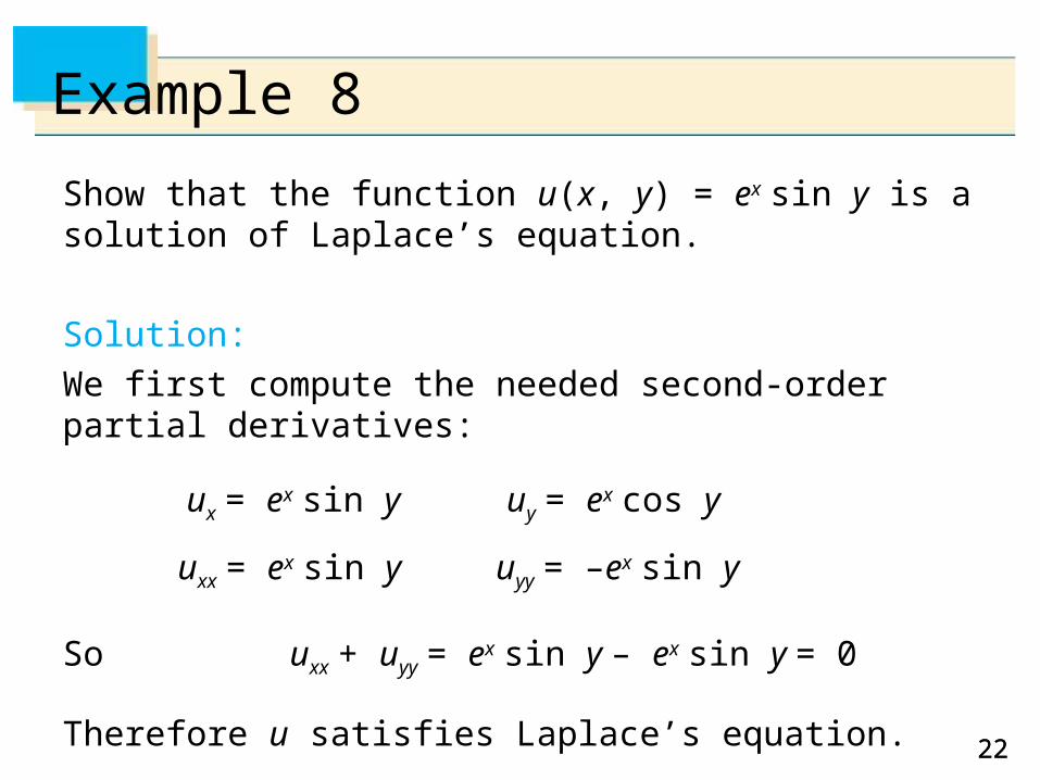
Example 8
Show that the function u(x, y) = ex sin y is a solution of Laplace’s equation.
Solution:
We first compute the needed second-order partial derivatives:
ux = ex sin y uy = ex cos y
uxx = ex sin y uyy = –ex sin y
So uxx + uyy = ex sin y – ex sin y = 0
Therefore u satisfies Laplace’s equation.


