33
Copyright © Cengage Learning. All rights reserved. Polar Coordinates and Parametric Equations
| Date post: | 17-Dec-2015 |
| Category: |
Documents |
| Upload: | chad-wells |
| View: | 222 times |
| Download: | 1 times |

Copyright © Cengage Learning. All rights reserved.
Polar Coordinates and Parametric Equations

Copyright © Cengage Learning. All rights reserved.
8.4 Plane Curves and Parametric Equations

3
Objectives
► Plane Curves and Parametric Equations
► Eliminating the Parameter
► Finding Parametric Equations for a Curve
► Using Graphing Devices to Graph Parametric Curves

4
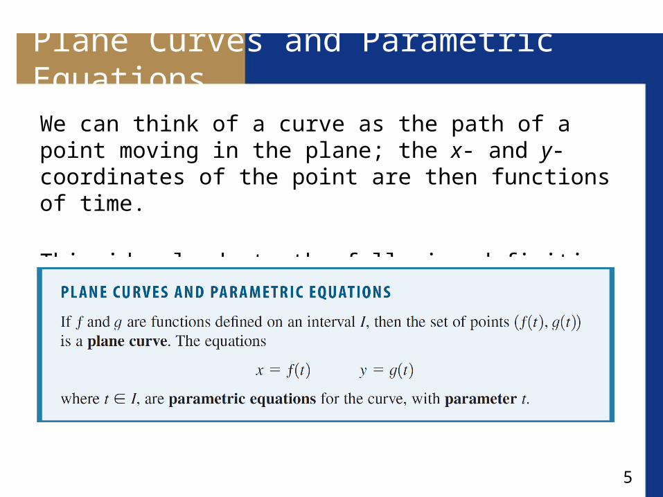
Plane Curves and Parametric Equations
In this section we study parametric equations, which are a general method for describing any curve.
5
Plane Curves and Parametric Equations
We can think of a curve as the path of a point moving in the plane; the x- and y-coordinates of the point are then functions of time.
This idea leads to the following definition.

6
Example 1 – Sketching a Plane Curve
Sketch the curve defined by the parametric equations
x = t2 – 3t y = t – 1
Solution:For every value of t, we get a point on the curve. For example, if t = 0, then x = 0 and y = –1, so the corresponding point is (0, –1).

7
Example 1 – Solution
In Figure 1 we plot the points (x, y) determined by the values of t shown in the following table.
Figure 1
cont’d

8
Example 1 – Solution
As t increases, a particle whose position is given by the parametric equations moves along the curve in the direction of the arrows.
cont’d
9
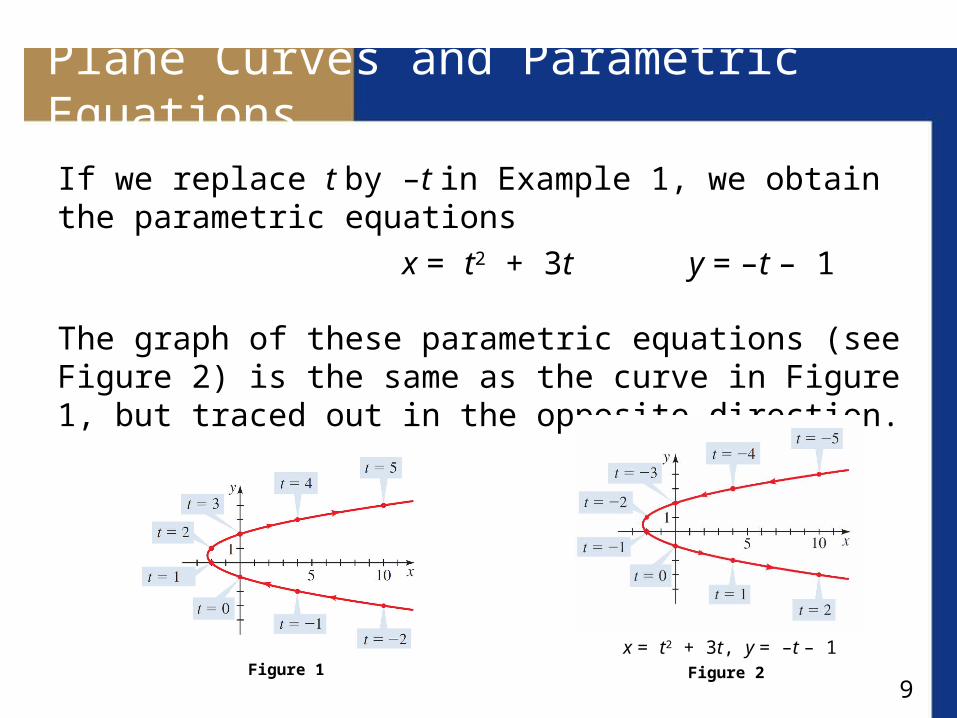
Plane Curves and Parametric Equations
If we replace t by –t in Example 1, we obtain the parametric equations
x = t2 + 3t y = –t – 1
The graph of these parametric equations (see Figure 2) is the same as the curve in Figure 1, but traced out in the opposite direction.
Figure 2
x = t2 + 3t, y = –t – 1Figure 1
10
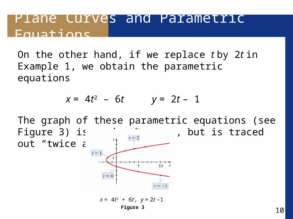
Plane Curves and Parametric Equations
On the other hand, if we replace t by 2t in Example 1, we obtain the parametric equations
x = 4t2 – 6t y = 2t – 1
The graph of these parametric equations (see Figure 3) is again the same, but is traced out “twice as fast.”
Figure 3
x = 4t2 + 6t, y = 2t –1

11
Plane Curves and Parametric Equations
Thus, a parametrization contains more information than just the shape of the curve; it also indicates how the curve is being traced out.

12
Eliminating the Parameter

13
Eliminating the Parameter
Often a curve given by parametric equations can also be represented by a single rectangular equation in x and y.
The process of finding this equation is called eliminating the parameter.
One way to do this is to solve for t in one equation, then substitute into the other.

14
Example 2 – Eliminating the Parameter
Eliminate the parameter in the parametric equations of Example 1.
Solution:First we solve for t in the simpler equation, then we substitute into the other equation.
From the equation y = t – 1, we get t = y + 1.

15
Example 2 – Solution
Substituting into the equation for x, we get
x = t2 – 3t = (y + 1)2 – 3(y + 1) = y2 – y – 2
Thus the curve in Example 1 has the rectangular equation x = y2 – y – 2, so it is a parabola.
cont’d

16
Finding Parametric Equations for a Curve

17
Example 5 – Finding Parametric Equations for a Graph
Find parametric equations for the line of slope 3 that passes through the point (2, 6).
Solution:Let’s start at the point (2, 6) and move up and to the right along this line.
Because the line has slope 3, for every 1 unit we move to the right, we must move up 3 units. In other words, if we increase the x-coordinate by t units, we must correspondingly increase the y-coordinate by 3t units.

18
Example 5 – Solution
This leads to the parametric equations
x = 2 + t y = 6 + 3t
To confirm that these equations give the desired line, we eliminate the parameter.
We solve for t in the first equation and substitute into the second to get
y = 6 + 3(x – 2) = 3x
cont’d

19
Example 5 – Solution
Thus the slope-intercept form of the equation of this line is y = 3x, which is a line of slope 3 that does pass through (2, 6) as required. The graph is shown in Figure 6.
Figure 6
cont’d

20
Example 6 – Parametric Equations for the Cycloid
As a circle rolls along a straight line, the curve traced out by a fixed point P on the circumference of the circle is called a cycloid (see Figure 7).
If the circle has radius a and rolls along the x-axis, with one position of the point P being at the origin, find parametric equations for the cycloid.
Figure 7

21
Example 6 – Solution
Figure 8 shows the circle and the point P after the circle has rolled through an angle (in radians).
The distance d(O, T ) that the circle has rolled must be the same as the length of the arc PT, which, by the arc length formula, is a.
Figure 8

22
Example 6 – Solution
This means that the center of the circle is C(a, a).
Let the coordinates of P be (x, y). Then from Figure 8 (which illustrates the case 0 < < /2), we see that
x = d(O, T) – d(P, Q) = a – a sin = a( – sin )
y = d(T, C) – d(Q, C) = a – a cos = a(1 – cos )
so parametric equations for the cycloid are
x = a( – sin ) y = a(1 – cos )
cont’d

23
Using Graphing Devices to Graph Parametric Curves

24
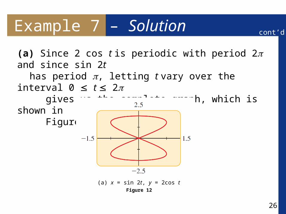
Example 7 – Graphing Parametric Curves
Use a graphing device to draw the following parametric curves. Discuss their similarities and differences.
(a) x = sin 2t
y = 2 cos t
(b) x = sin 3t
y = 2 cos t

25
Example 7 – Solution
In both parts (a) and (b) the graph will lie inside the rectangle given by –1 x 1, –2 y 2, since both the sine and the cosine of any number will be between –1 and 1.
Thus, we may use the viewing rectangle [–1.5, 1.5] by
[–2.5, 2.5].
26
Example 7 – Solution
(a) Since 2 cos t is periodic with period 2 and since sin 2t has period , letting t vary over the interval 0 t 2 gives us the complete graph, which is shown in Figure 12(a).
Figure 12
(a) x = sin 2t, y = 2cos t
cont’d

27
Example 7 – Solution
(b) Again, letting t take on values between 0 and 2 gives the complete graph shown in Figure 12(b).
Figure 12
(b) x = sin 3t, y = 2cos t
cont’d

28
Example 7 – Solution
Both graphs are closed curves, which means they form loops with the same starting and ending point; also, both graphs cross over themselves.
However, the graph in Figure 12(a) has two loops, like a figure eight, whereas the graph in Figure 12(b) has three loops.
cont’d

29
Using Graphing Devices to Graph Parametric Curves
The curves graphed in Example 7 are called Lissajous figures. A Lissajous figure is the graph of a pair of parametric equations of the form
x = A sin ω1t y = B cos ω2t
where A, B, ω1, and ω2 are real constants. Since sin ω1t and cos ω2t are both between –1 and 1, a Lissajous figure will lie inside the rectangle determined by –A x A, –B y B.

30
Using Graphing Devices to Graph Parametric Curves
This fact can be used to choose a viewing rectangle when graphing a Lissajous figure, as in Example 7.
We know that rectangular coordinates (x, y) and polar coordinates (r, ) are related by the equations x = r cos , y = r sin .
Thus we can graph the polar equation r = f() by changing it to parametric form as follows:
x = r cos = f() cos Since r = f()

31
Using Graphing Devices to Graph Parametric Curves
y = r sin = f() sin
Replacing by the standard parametric variable t, we have the following result.
32
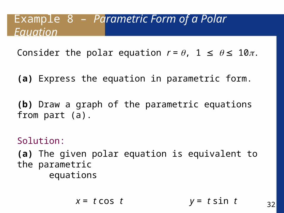
Example 8 – Parametric Form of a Polar Equation
Consider the polar equation r = , 1 10.
(a) Express the equation in parametric form.
(b) Draw a graph of the parametric equations from part (a).
Solution:
(a) The given polar equation is equivalent to the parametric equations
x = t cos t y = t sin t
33
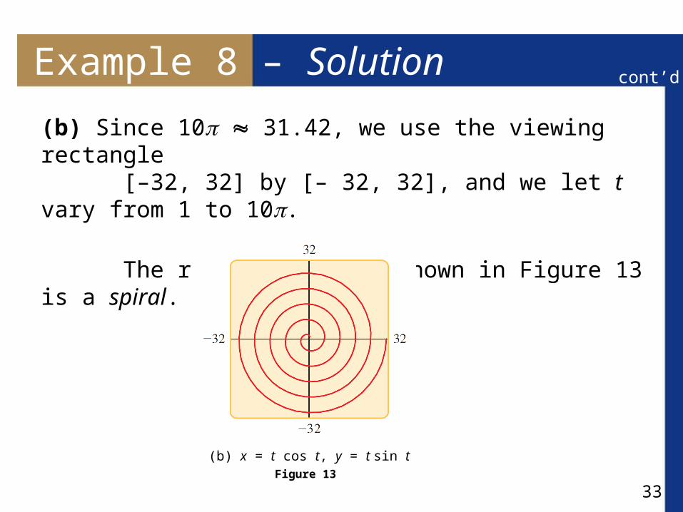
Example 8 – Solution
(b) Since 10 31.42, we use the viewing rectangle [–32, 32] by [– 32, 32], and we let t vary from 1 to 10.
The resulting graph shown in Figure 13 is a spiral.
Figure 13
(b) x = t cos t, y = t sin t
cont’d


