*Research Professor and Director Surveys of Consumers, University of Michigan. E-mail: [email protected]National Bank of Poland December 2005 Warsaw, Poland Inflation Expectations: Theoretical Models and Empirical Tests Richard Curtin 1 * The University of Michigan data on consumers’ inflation expectations has been analyzed by a wide range of scholars for nearly fifty years. The empirical evidence has been mixed about the extent to which inflation expectations are consistent with the rational expectations hypothesis of traditional economic models or with the bounded rationality postulate of the newer behavioral models. Even if expectation were rational, judgements about the costs and benefits of continuously updating inflation expectations may result in sticky or staggered information flows that may make expectations appear non-rational. Importantly, sticky expectations, like sticky wages and sticky prices, can have a significant impact on optimal monetary policy. The Michigan data on inflation expectations is used to test a wide range of hypothesis surrounding these basic issues, utilizing cross-section, panel, and time-series data. The analysis indicates that there exists considerable heterogeneity in inflation expectations, that inflation expectations are forward looking, that consumers do not efficiently utilize all available information, that negative changes in the inflation rate have about twice the impact as positive changes, that there is evidence of staggered updating, and that these findings do not result from offsetting errors across demographic groups. Realism and Relevance John Muth began his classic article on rational expectations by noting that survey data on expectations were as accurate as the elaborate models of economists, and he noted that there were considerable differences of opinion in the cross-sectional survey data (Muth, 1961). His basic insight was that economic agents form their expectations so that they are essentially the same as the predictions of the relevant economic theory. The assumption that expectations were formed rationally was for Muth the natural extension of economic theory which already held that firms rationally maximize profits and consumers rationally maximize utility. Nonetheless, Muth noted that rationality was an assumption that could be tested by its systematic comparison with alternative theories in explaining observed expectations. Muth’s hypothesis has indeed sparked an enormous amount of research as well as wide divisions between disciplines in how rationality should be conceptualized and how the hypothesis should be tested. Economics views rationality in terms of the choices it produces (substantive or full rationality), whereas other social sciences view rationality in terms of the process that is used to make choices (procedural or bounded rationality). It was Friedman’s (1953) celebrated essay on methodology that declared the validity of economic theories to be independent of their psychological assumptions. Economists have accordingly focused on whether the postulate of
Transcript
*Research Professor and Director Surveys of Consumers, University of Michigan. E-mail: [email protected]
National Bank of Poland December 2005Warsaw, Poland
Inflation Expectations: Theoretical Models and Empirical Tests
Richard Curtin1*
The University of Michigan data on consumers’ inflation expectations has beenanalyzed by a wide range of scholars for nearly fifty years. The empirical evidence has beenmixed about the extent to which inflation expectations are consistent with the rationalexpectations hypothesis of traditional economic models or with the bounded rationalitypostulate of the newer behavioral models. Even if expectation were rational, judgementsabout the costs and benefits of continuously updating inflation expectations may result insticky or staggered information flows that may make expectations appear non-rational.Importantly, sticky expectations, like sticky wages and sticky prices, can have a significantimpact on optimal monetary policy. The Michigan data on inflation expectations is used totest a wide range of hypothesis surrounding these basic issues, utilizing cross-section, panel,and time-series data. The analysis indicates that there exists considerable heterogeneity ininflation expectations, that inflation expectations are forward looking, that consumers do notefficiently utilize all available information, that negative changes in the inflation rate haveabout twice the impact as positive changes, that there is evidence of staggered updating, andthat these findings do not result from offsetting errors across demographic groups.
Realism and Relevance
John Muth began his classic article on rational expectations by noting that survey data onexpectations were as accurate as the elaborate models of economists, and he noted that therewere considerable differences of opinion in the cross-sectional survey data (Muth, 1961). His basicinsight was that economic agents form their expectations so that they are essentially the same asthe predictions of the relevant economic theory. The assumption that expectations were formedrationally was for Muth the natural extension of economic theory which already held that firmsrationally maximize profits and consumers rationally maximize utility. Nonetheless, Muth noted thatrationality was an assumption that could be tested by its systematic comparison with alternativetheories in explaining observed expectations.
Muth’s hypothesis has indeed sparked an enormous amount of research as well as widedivisions between disciplines in how rationality should be conceptualized and how the hypothesisshould be tested. Economics views rationality in terms of the choices it produces (substantive orfull rationality), whereas other social sciences view rationality in terms of the process that is usedto make choices (procedural or bounded rationality). It was Friedman’s (1953) celebrated essayon methodology that declared the validity of economic theories to be independent of theirpsychological assumptions. Economists have accordingly focused on whether the postulate of
2Many economists have now reinterpreted Muth’s original hypothesis to apply at the micro rather than an the aggregate level(Begg, 1982). They reasoned that given that utility maximization is assumed to be true for each individual, why shouldrational expectations be exempted from micro testing? Some analysts have even claimed that the only appropriate test ofthe rational expectations hypothesis would be based on panel data. Some have also argued that the aggregation involvedin time-series tests result in inconsistent estimates and masks offsetting individual differences (Figlewski and Wachtel, 1983;Keane and Runkle, 1990).
2
unbounded or bounded rationality was the more productive theoretical construct in terms of itspredictive accuracy.
Compared with tests of utility maximization, expectations have the unique advantage thatthey could be measured and subjected to empirical tests.2 The rigor of the tests of the rationalexpectations hypothesis ranges from tests of bias and predictive accuracy to how efficiently everypossible piece of relevant information was used in forming the expectations. There is a virtualabsence of empirical tests of the assumptions surrounding utility maximization, including tests onwhether agents gather and process the relevant economic information and to use it efficiently tomaximize utility, and whether consumers know all the relevant facts at any given time or if thereexits informational heterogeneity.
There are some economist that take seriously the implicit assumptions that there arenegligible costs associated with collecting and processing all the relevant information and that allagents know the correct dynamic model. When asked about the stringent assumptions surroundingutility maximization, economists quickly allow that what those simplifying assumptions lack inrealism they make up for in predictive performance. The lack of such a recognition of Friedman’sbasic methodological points in the discussion of rational expectations is quite amazing.
It should not be surprising that the debate about the rational expectations hypothesis hascontinued unabated in the nearly fifty years since Muth first published his theory. Perhaps it is asLovell (1986) lamented two decades ago in his review of empirical tests of the rational expectationshypothesis, “...why should data spoil such a good story.” Indeed, the clear advantage of the rationalexpectations hypothesis is its theoretical strength. The hypothesis has proved to be enormouslyproductive in transforming macroeconomic theory given that the rationality assumption enables thepowerful tools of optimization to systematically expand the depth and breath of economic theories.
While the empirical tests have generally not fully supported the hypothesis, the criteria foracceptance are rigorous and the lack of evidence is comparable to that found in tests of the fullrationality postulate in many other aspects of economic theory. In contrast, while boundedrationality has frequently been confirmed in empirical studies, research on bounded rationality hasnot led to an integrated theoretical structure that could spark further theoretical advances. Indeed,the findings attributable to bounded rationality have been generally classified as “anomalies” ratherthan being incorporated into mainstream theory. The list of such anomalies includes the impact offraming, asymmetry of gains and losses, relative reference points, anchoring, and confirmatory bias,among other findings (Tversky & Kahneman, 1982; Earl, 1990; Thaler, 1991; Thaler, 1992; Rabin,1998; Rabin & Schrag, 1999). Only recently has there been a concerted effort to incorporate amore realistic account of expectations into mainstream economic theory rather than relegating themto anomaly status.
3
Costs and Benefits ofRational Expectations
Like most economic phenomena, inflation expectations can be integrated into mainstreamtheory by the systematic recognition of the costs and benefits associated with rational expectations.Rational expectations are costly to form and their benefits are derived from their use in economicdecisions. As long as there is any positive cost involved in collecting and processing informationusing the relevant dynamic model, some agents will choose to sometimes hold less accurateexpectations. The terms “sticky information” or “rational inattention” have been used to describethe impact of costs on the formation process (Mankiw and Reis, 2002; Sims 2003; Bacchetta andWincoop, 2005). These theories postulate that rational consumers may find the costs associatedwith updating their expectations to exceed the benefits. At any given time some people will find itworthwhile to incur the costs, especially if that information is critical to a pending decision. Mostof the time, however, rational inattention is the optimal course. Alternatively, agents may base theirexpectations on imperfect information, which can be conceptualized as less costly than perfectinformation. Whatever the cause, the process creates staggered changes in expectations, wherebyat any given time expectations reflect a combination of current and past information across differentpeople.
Disagreement across people in their expectations at any given time is taken as an indicationof such a process (Mankiw, Reis and Wolfers, 2004). Some have modeled the disagreements asthe result of factors other than costs, such as an epidemiological process in which “expert opinion”spreads slowly through a population like the spread of a disease (Carroll, 2003) . Costs can alsobe assumed to vary across demographic subgroups, as some encounter lower costs for acquiringand using information, and other more economically active subgroups derive greater benefits fromupdating their expectations more frequently. This interpretation of disagreements or inaccuraciesin expectations stands in contrast to the older and still more common interpretation that the veryexistence of differences across demographic subgroups indicate non-rational expectations (Bryanand Venkatu, 2001; Souleles, 2001).
Staggered changes could be created by a wide range of processes that either encourageor discourage agents from updating their expectations. A common hypothesis hold that it is dueto asymmetric responses to economic information, with agents updating their expectations muchmore quickly in response to bad news about inflation. Akerloff, Dickens and Perry (2001) suggestthat bad economic news is perceived by consumers to contain more potentially relevant informationabout their financial situation. The volume of news also matters, especially the volume of badnews, as well as news that represent a sharp and negative break from the past (Carroll, 2003).Sims (2003) shows that based on information theory the tone and volume of economic reportingaffects expectations beyond the information contained in the reports. This added impact of news,however, may be short-lived, usually lasting less than a few months (Doms and Morin, 2004).
It is not clear when the news media creates expectations and when its reporting simplyresponds to ongoing changes in expectations. Like any other business, the news media caters toconsumers’ preferences (Hamilton, 2004). For example, large shifts in expectations for futurechanges in the unemployment rate were found to change in advance of shifts in media reportsabout unemployment (Curtin, 2003).
The same staggered information flows have been hypothesized to result from uncertaintyabout the correct structural model of the economy. Since model uncertainty is costly to resolve, it
4
results in less frequent updating of expectations (Branch, 2005). Although the data that indicatesdisagreement in expectations is similar to what could be expected to result from model uncertainty,these two concepts are distinct. More importantly, the prevalence of disagreement may be muchmore variable over time than uncertainty.
The models developed to capture the impact of staggered information are similar toconsumption models that incorporate the division between “rule of thumb” and rational consumers.In this context, the switching models capture the difference between those that update theirexpectations regularly and those that base their expectations on pre-existing information. Mankiwand Reis (2003), Carroll (2003), and Khan and Zhu (2002) estimated that rather than continuouslyupdating their expectations, most people update their expectations only a few times a year.
Sticky information theories result in differences in inflation expectations across agents.There are, however, other reasons to expect heterogeneity that represent more fundamental issues.Conventional economic theory assumes that the same information is available to all agents and thesame models are used to generate expectations about the future. The result is that there is onlyone rational expectation at any given time for a given information set. Thus, while staggeredinformation and model uncertainty may result in heterogeneity of expectations, there is notheoretical basis for expecting heterogeneity among those that have recently updated theirexpectations. The allowance of private information in addition to public and official information toinfluence the formation of expectations would provide a theoretical reason for heterogeneity inexpectations. For example, the impact of private information has been found to be pivotal in theformation of unemployment expectations (Curtin 2003).
Monetary Policy ImplicationsOf Staggered Information Flows
Whatever the cause, the presence of sticky information is hypothesized to be the key tounderstanding dynamics of the macro economy. Sticky information has a long history in researchon forward-looking Phillips curves (Woodford, 2003). The sticky information has ranged fromstaggered wage contracts, to staggered pricing models, and to staggered information flows.Whatever the source, the existence of sticky information indicates the non-neutrality of monetarypolicy.
While there is now a widespread belief that monetary policy can influence output andemployment, there is no consensus on the mechanisms that produce the impact. To be sure, ifinflation expectations were fully rational and the central bank was fully committed to price stability,there would be no impact on output and employment. Non-neutrality derives from non-rationalityin expectations or from a lack of commitment to price stability on the part of the central bank.
The optimal situation is when the central bank enjoys widespread credibility andexpectations are fully rational, allowing the central bank to reduce inflation without any loss inoutput or employment. Although central banks differ widely in the credibility they enjoy, evenamong those that have the highest credibility economic losses cannot be completely avoided.
When those optimal conditions are not present, expected inflation can become self-fulfillingdue to what has been termed the “expectations trap” (Chari, Christiano and Eichenbaum, 1998;Albanesi, Chari and Christiano, 2002; Leduc, Sill and Stark, 2003). The enticement into the trap
3Plato wrote that “...each man possesses opinions about the future, which go by the general name of expectations...” (Plato,Laws 644c, 360 BC).
5
is the higher cost in terms of output and employment that would result following the choices alreadymade by households and firms in anticipation of higher inflation: consumers typically favor debtwhose repayment will be eroded by higher inflation, and firms typically raise prices in advance toprotect the real value of their profits. These actions would imply relatively larger future losses inoutput and employment if the central bank adopted a policy aimed at price stability. Since theactions already taken by both consumers and firms act to lower the costs of inflation, the centralbank is “trapped” into an accommodative policy that confirms the higher inflation expectations.
While full rationality and a fully committed central bank may seem too much to expect,Woodford (2005) advanced the notion that the main conclusions for optimal monetary policy alsopertain to the assumption of near-rational expectations. While there is no accepted standard tojudge whether expectations are “near-rational,” the analysis of inflation expectations can help to sortout the various properties of expectations.
This paper investigates a broad range of these issues, including whether inflationexpectations are backward or forward looking, whether there is any support for the staggeredinformation hypothesis, the interpretation of disagreement data, and some other methodologicalissues. Prior to the analytic sections, the rational expectations model as well as the adaptationmodels are defined. The analysis then turns to the analysis of household inflation expectationscollected by the University of Michigan, variously based on cross-section data, panel data, andtimes-series data. Finally, the analytic results are discussed along with their implication formonetary policies.
Theoretical Models of Expectations
Expectations are beliefs about the future. This definition was cited by Plato more than twothousand years ago, and it remains to this day the generally accepted meaning of the term.3 Theformation of expectations depends on two factors: informational inputs (I) and the model or processof transforming information into expectations (f). Let the expectation of the inflation rate (Pe) formedby the ith individual be defined as:
where the subscript t on Pe indicates the period for which the expectation applies, and theexpectation formed based on the information that was available in a prior period, denoted by et-1.The two dominant specifications of this equation are the rational expectations hypothesis and theextrapolative, adaptive, and error learning models, which I will refer to collectively as “adaptive”expectations.
The format of the appropriate empirical tests of these two models is just as distinctive astheir assumptions about rationality. The adaptive expectations models define what information isused and how it is used in the formation of expectations, including the availability and cost ofinformation as well as the capacity of individuals to effectively utilize the information. The empirical
P f Ite
tt − = −
11( )
6
tests were designed to determine whether variations in expectations are related to thesehypothesized factors. In contrast, tests of the rational expectations hypothesis focus on whetherthe observed expectations are unbiased future forecasts and whether all of the information wasused efficiently and optimally. In the former case, expectations are analyzed as the dependentvariable, while in the latter case expectations are viewed as an independent variable in the analysis.
This difference makes the comparison of the relative merits of the two models difficult. Forthe adaptive expectations models, confirmation essentially entails finding a significant empiricalrelationship between expectations and some informational inputs. Confirmation of the rationalexpectations hypothesis, in contrast, requires the finding of unbiased and efficient futurepredictions. In tests of adaptive expectations, any statistically significant finding is taken asconfirmation even if it accounts for a trivial proportion of the variance, whereas anything short of fullrationality requires the rejection of the rational expectations hypothesis. This asymmetry in theevaluation of empirical evidence has stunted theoretical developments.
This situation is nowhere more important than in the assessment of the forward-lookingcontent of expectations. Adaptive expectations models are inherently bound to the past. Asidefrom the special case where future outcomes are extrapolations of the past, no method is usuallyhypothesized to test the forward-looking content of expectations. Indeed, by their very construction,adaptive expectations models portray the formation process as a relatively transparent function ofpast outcomes where individuals never fully learn from their past errors. Rational expectationsmodels, in contrast, place their entire emphasis on assessing the forward-looking information, butdo not posit any specific process for the formation of expectations. When empirically rejected, therational expectations framework provides no insight into which limitations on rationality proved tobe most important.
Adaptive Expectations. The various adaptive, extrapolative, and error learning models canbe summarized by the following autoregressive distributive lag representation:
where Pe is inflation expectations, P is the actual inflation rate, j is the lag length, and ε is the errorterm, with the i subscript dropped for convenience. Variables other than the inflation rate that arepart of the relevant information could also be included in the equation. Defining the uniquecharacteristics of the various models involves the specification of coefficients β, γ, and ε.
Perhaps the most basic hypothesis is that expectations essentially represent randomresponses to the survey questions, unrelated to either the past realizations of the variable or evenpast expectations. In this case, the β, and γ coefficients would be hypothesized to be equal to zero,so that variations in expectations about its mean (α) are simply equal to the error term.
The pure extrapolative model is obtained by setting the coefficients β equal to zero, so thatexpectations solely depend on the lagged inflation rate. The most restricted version of this modelcan be characterized as “static expectations,” where expectations simply depend on the mostrecent realization. The more general version holds that expectations represent a weighted averageof past realizations. Under the extrapolative hypothesis, the γ coefficients are hypothesized to beany positive fraction between zero and one.
P P Pte
j t je
jj
jt j t= + + +− −∑ ∑α β γ ε
7
The adaptive or error learning hypothesis posits that consumers revise their expectationsfor the following period based on the error in their expectations in the current period (Fisher 1930,Cagan 1956, Friedman 1957, Nerlove 1958). In terms of the above equation, this implies that onlyone lag of the actual and expectation variables are used, with the coefficient on the differencebetween the expected and actual outcomes (the speed of the learning adjustment) hypothesizedas being positive with an upper bound of 1.0. By use of the Koyck (1954) transformation, however,the adaptive expectations model can be shown to be equivalent to a weighted average of pastrealizations.
Another approach has been to utilize error correction models, which postulate equality inequilibrium between inflation expectations and the inflation rate. The basic error correction modelcan be expressed by using one lag of the expectations variable and two lags of the actual inflationrate, and fixing these coefficients at 1.0 to express the notion that the equilibrium rate of inflationis equal to its expectation. The error correction equation thus relates the change in expectationsto past changes in the actual inflation rate as well as the error in the prior period’s expectation.
The reliance on information about past changes in inflation is the source of the mostimportant disadvantage of all adaptive expectations models because systematic prediction errorsresult since expectations tend to underestimate (overestimate) the true change whenever theunderlying variable is trending upward (downward). In response to this deficiency, augmentedmodels have been proposed, which incorporate information on other variables that are assumedto influence the formation of expectations. The use of this additional information can help to offsetthe tendency toward systematic prediction errors.
Rational Expectations. The strong appeal of the rational expectations hypothesis is thatit avoids the bias toward systematic prediction errors by shifting its focus from the variable’s historyto its future realizations. The rational expectations hypothesis equates the expectation with theexpected value of the actual subsequent realization, conditional on all available information (Muth,1961). Unbiased expectations under the rational expectations hypothesis require that thecoefficients α and β are zero and one, respectively, in the equation:
The strong test of rationality also requires that all of the available information has been efficientlyand optimally used in forming the expectation. This involves tests on the statistical properties of theprediction errors to determine if they are consistent with those stipulated by the hypothesis(orthogonality, efficiency, consistency, as well as unbiasedness). Tests of this assumption take theform:
where ζ is the prediction error, the coefficients β and γ are expected to be zero, and the predictionerrors are serially uncorrelated. This expresses the notion that if any of the available informationwas systematically related to the prediction errors, the information was not efficiently and optimallyincorporated into the formation of the original expectation.
P Pt te
tt= + +−α β ε1
ζ α β γ εt j t j j t j tP Z= + + +∑ ∑− −
8
Reification of Economic DataIn Tests of Expectations
Some economists seem to believe the only source of information about the actual inflationrate is the official announcements by the government’s statistical agency. The assumption thatconsumers only utilize official sources of economic information reflects the widespread tendencytoward the reification of economic data—that is, treating conceptual measures as if they had aconcrete existence. All economic data represent estimates of the underlying concepts, and someprice indexes are measured with more error than others. There is no evidence that consumersrevise their inflation expectations each time the government issues new monthly estimates, revisesold figures or revises its measurement methodology. More importantly, aside for those who havetheir incomes or pensions indexed to official indexes, theory suggests that consumers will usewhatever measure that best reflects their own expenditures. It would make no sense for consumersto take into account future prices that they will not face when making decisions.
The recent debate about whether tests on inflation expectations should be based on realtime data or revised data reflects this tendency toward the reification of data (Mehra, 2002;Croushore and Stark, 1999; Keane and Runcle, 1989; Zarnowitz, 1985). The information set at anygiven time is usually assumed to only include past data on the official inflation rate, usually outdatedby at least one month (the official release of U.S. data on the Consumer Price Index (CPI) for anygiven month is by the middle of the following month). While economist may condition their forecastsonly on official data, consumers can be expected to actively use all the information available tothem to gauge ongoing changes in price trends. Rather than relying on official information,consumers more often report and depend on private information.
If anything, consumers suffer from an overload of private information about prices. Incomparison to the official information which has been released once a month in nearly the sameformat for decades, private information has increased substantially. The media has beenrepeatedly reinvented to provide expanded information, from newspapers, to television, to 24/7operations of cable news, the internet, and the self-proclaimed experts that now inhabit all media.More importantly, people gain information on prices in every daily transaction in the marketplace.This personal collection of information is typically reported by consumers to be the most critical tothe formation of their expectations.
One way of exploring the impact of private versus official information is to compare changesin expectations with the official release dates. The key analytic issue is how to devise a proxymeasure of the unobserved inflation rate prior to the official announcement. This issue is easy tosolve: the best estimate of the current month’s inflation is the official inflation rate. And thehypothesis could be easily tested: the current month’s price index should be dominated by lastmonth’s inflation index for the official information hypothesis to hold, and the current month’s priceindex should dominate last month’s official release if private information dominates. As youprobably already know, such a test provides little support for the notion that consumers base theirexpectations on the official announcement.
The last issue is which inflation rate is the most appropriate to use to model consumerexpectations? The inflation index most often favored by economists is a core rate that excludesenergy and food prices, and is either based on the consumer price index or the personalconsumption deflator. Consumers generally identify inflation with the overall consumer price indexor personal consumption deflator as they best capture the prices of the goods and services that
9
they actually purchase. This analyses included in this paper focus on changes in the overallConsumer Price Index (CPI-u).
Data on Inflation Expectations
The University of Michigan has collected data on the inflation expectations of consumersfor more than fifty years. Two questions are now asked of all consumers about expected pricechanges: the expected direction of change in prices and the expected extent of change. Thequestion on the expected direction of change has been asked in a comparable format since 1946,while the question on the extent of change has been modified several times. In the 1940's and1950's, the question simply asked whether prices would go up a little or go up a lot; from the 1960'sto the mid 1970's, the question included a series of fixed percentage intervals from which therespondent was asked to choose; and from the mid 1970's to present, the question simply askedthe percent rate of inflation that the consumer expected. This paper focuses only on the monthlydata collected since 1978 for the open-ended question on inflation expectations.
There is a considerable degree of cross-section as well as time-series variation inconsumers’ responses. The variation in responses is due to a number of factors, includingdifferences in information and computational capacities, uncertainty about the correct dynamicmodel, and measurement errors. These differences are discussed from several perspectivesbased on cross-section, time-series, and panel data.
Cross-Section Variation in Responses
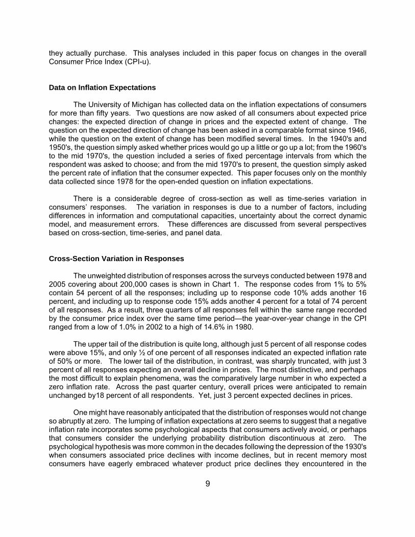
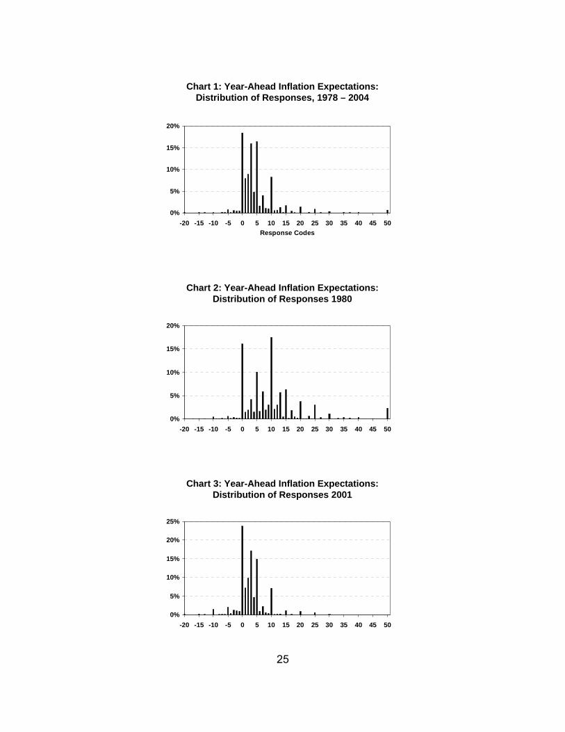
The unweighted distribution of responses across the surveys conducted between 1978 and2005 covering about 200,000 cases is shown in Chart 1. The response codes from 1% to 5%contain 54 percent of all the responses; including up to response code 10% adds another 16percent, and including up to response code 15% adds another 4 percent for a total of 74 percentof all responses. As a result, three quarters of all responses fell within the same range recordedby the consumer price index over the same time period—the year-over-year change in the CPIranged from a low of 1.0% in 2002 to a high of 14.6% in 1980.
The upper tail of the distribution is quite long, although just 5 percent of all response codeswere above 15%, and only ½ of one percent of all responses indicated an expected inflation rateof 50% or more. The lower tail of the distribution, in contrast, was sharply truncated, with just 3percent of all responses expecting an overall decline in prices. The most distinctive, and perhapsthe most difficult to explain phenomena, was the comparatively large number in who expected azero inflation rate. Across the past quarter century, overall prices were anticipated to remainunchanged by18 percent of all respondents. Yet, just 3 percent expected declines in prices.
One might have reasonably anticipated that the distribution of responses would not changeso abruptly at zero. The lumping of inflation expectations at zero seems to suggest that a negativeinflation rate incorporates some psychological aspects that consumers actively avoid, or perhapsthat consumers consider the underlying probability distribution discontinuous at zero. Thepsychological hypothesis was more common in the decades following the depression of the 1930'swhen consumers associated price declines with income declines, but in recent memory mostconsumers have eagerly embraced whatever product price declines they encountered in the
4The larger variance that has often been associated with higher expected inflation rates in the literature, may be partially dueto the truncation of the distribution at zero.
5Transforming the qualitative expectations into quantitative estimates has been done for inflation expectations with mixedsuccess. Different methods have been used to “quantify” qualitative measures of expectations, with the Carlson-Parkin(1975) technique the most widely known. These techniques involve an assumption about the underlying and unobserveddistribution of expectations (typically assumed normal, but other distributional assumptions have been used) combined withan assumption that across the entire time-series expectations are unbiased and equal realizations (although other identifyingassumptions are possible). See Batchelor (1986) and Pesaran (1987) for a review of these techniques.
10
marketplace. The single, and important, exception being home prices. Rather than a kink in theunderlying probability distribution, the lumping at zero may simply reflect rounding, with consumersactually expecting a very low rate of inflation and not price declines.
The truncation does not reflect the averaging of a few surveys where expectations ofdeclines were common with the many more surveys where they were uncommon. Chart 2 showsthe response distribution for 1980, when inflation expectations were at their highest levels; Chart3 shows the response distribution for 2001, when inflation expectations were at their lowest levels.The same truncation in response is evident in both cases. The major difference is that the 1980distribution is shifted to the right and has a greater dispersion of responses.4
Whatever the cause, the data clearly indicate a truncated lower tail rather than a normaldistribution. Importantly, the extent of the truncation provides important information for thoseutilizing distribution assumptions to calculate a numerical estimate from qualitative response scaleson inflation expectations, as is commonly done among EU countries.5
Digit Preference
A close examination of the response distribution indicates the prevalence of certain digits,namely 0, 5, 10, 15, 20, and so on up to 50. This tendency to favor certain digits has been termed“digit preference.” Digit preference is a widespread phenomena, exhibited in nearly all responsesto open-ended numeric questions (Baker, 1992; Edouard and Senthilselvan, 1997). The questionscould ask about dollar amounts of income, assets, debts, product prices, or questions aboutprobabilities of the occurrence of certain events, from the weather to a variety of economic orpolitical outcomes, and even in response to attributes of the person such as weight. The typicalexplanation of digit preference is that it represents “rounded” answers based on considerations ofthe cost of providing more exact responses. Economists may favor a “near rationality”interpretation whereby the rounding represents the level of precision that is associated withdifferences that matter to the respondent.
An even closer inspection will reveal the prevalence of 3, 7, 13, 17, and so on. This reflectscoding rules implemented by the survey organization to provide a consistent means to code rangeresponses. All responses are recorded as integers, and the very few decimal responses arerounded and coded as integers without any fractional values. The key part of the rule states thatcoders should round .5 to the nearest odd number, e.g. 3.5 would be rounded to 3 and 4.5 roundedto 5. This rule in combination of the prevalence of range responses produces the high prevalenceof the coded values 3, 7, 13 and so forth: for example, a response of 5% to 10% would be coded7%, a response of 10% to 15% would be coded 13%. Overall, the number of range responses arequite rare. Whenever a respondent would give a range response, it was always probed for a more
6There is a long standing debate about whether large estimates (say, five or more times the median or mean) should bedeleted and thus treated as missing data, or whether some information can be retained, namely that the respondent expecteda large increase, and the data should simply be truncated.
7The correlation between the interquartile range and the variance of the mean was 0.82.
11
exact point estimate in the Michigan surveys, but some respondents insisted that they could notnarrow the range to a single best integer estimate.
Digit preference and the frequency of range responses are usually considered surveymeasurement errors, given that they result in less precise measures. Experiments have beenconducted with the data before rounding (from one decimal) and the characteristics of the responsedistribution have been nearly identical to the rounded figures, as one would expect. Rangeresponses are likely to reflect uncertainty about the future course of inflation, or the lack ofinformation that a more precise answer would require (presumably due to its high cost).
Some have misinterpreted digit preferences as “focal points” in the distribution, and suggestthat this indicates that inflation expectations are more qualitative than quantitative in nature (Bryanand Palmqvist, 2005). The near universal presence of digit preferences would mean that the sameconclusion would be equally as valid for measures of income, assets, prices, and so forth, meaningthat surveys could measure only qualitative variables. The stability of the same integers as “focalpoints” in the distribution over time has been misinterpreted as indicating that the distribution ofresponses was not responsive to changes in the inflation or policies pursued by the central bank.
Time Series Variation
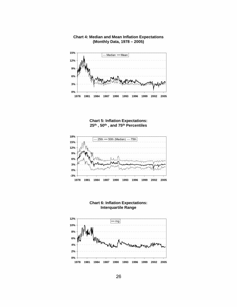
Rather than focusing on cross-section data, most economists are more interested in howthe distribution changes from month-to-month. Given the pronounced skew in the distribution ofinflation expectations, it is no surprise that the mean of the distribution always exceeds the median.Moreover, given that the long upper tail of the distribution is likely to represent measurement errors,the median rather than the mean of the distribution may provide the better measure of centraltendency.6 Indeed, the difference between the mean and median was substantial, with the meanbeing about 25% higher than the median, or 1.0 percentage points higher (see Chart 4). Over theperiod from January 1978 to August 2005, the mean of the monthly distributions was 4.8% whilethe median was 3.8%. Despite the difference in the levels, the time series correlation between themean and median was 0.98, indicating that either measure provided nearly identical time-seriesinformation. The median inflation expectation is typically the measure of choice, and I will restrictmy focus to the median in this paper.
The interquartile difference, defined as the difference between the 25th and 75th percentiles,can be used as an estimate of the variance in the monthly data.7 Over the 1978 to 2005 period,the interquartile range averaged 4.7 percentage points, with the 25th percentile averaging 1.5percentage points and the 75th percentile averaging 6.2 percentage points, meaning that half of allrespondents held expectations within that range. The time-series correlations were quite high, asthe correlation between the 25th percentile and the median was 0.91 and the correlation betweenthe 75th percentile and the median was 0.97 (see Chart 5).
12
The interquartile range provides some interesting information about trends in inflationexpectations. Increases in the variance occur abruptly, but decreases take place over an extendedtime period. Perhaps the clearest example in the sudden increase in variance at the time of the firstwar with Iraq in 1991. Following that increase, the variance of inflation expectation decreasedgradually over the next decade (see Chart 6). Central banks have interpreted this to indicate thattheir credibility can be lost suddenly, which then takes a considerable period of time to re-establish.
What do the cross-section as well as time-series variations in inflation expectationsindicate? There have been some that have used these variations as a strong indicator of vastmeasurement error, making the data worthless. Others, as I have already noted, interpret thevariations as a reflection of the costs of collecting and processing information which result in astaggered updating across respondents. While the more extreme responses may well reflectmeasurement errors, most of the disagreement or heterogeneity reflects the balancing of costs andbenefits of updating expectations. To explore these issues in more detail, repeated measures onthe same individuals is needed.
Panel Data on Expectations
The sample design of the monthly Surveys of Consumers includes a rotating panel. In therotating panel design, each monthly sample is composed of a new representative subsample aswell as a re-interview subsample of all respondents who were first interviewed six months earlier.The design was chosen to enhance the study of change in expectations and behavior. In thepresent context, the sample design means that for each respondent two measures of inflationexpectations were collected six months apart. In each interview, respondents were asked aboutthe expected inflation rate during the following twelve months. As a result, the two instances of thequestion do not ask about identical time periods but do contain overlapping periods of six months.
This design enables a partial test of the hypothesis of staggered information flows. Thestaggered information hypothesis suggests that in any given monthly survey only some of therespondents would have updated their expectations. For this analysis, the sample was restrictedto range from January 1993 to August 2005, when the inflation rate was more stable, averaging2.5%. More importantly, the average change in the actual inflation rate over all six month intervalswithin this time period was nearly zero, or more exactly 0.0005 percentage points. In comparison,the average change in inflation expectations among identical individuals was -0.247, or a decreaseof one-quarter of a percentage point. The negative change in inflation expectations probablyreflects the persistent declines in the inflation rate over the 1993 to 2005 period. Overall, given thatthe consumer data on inflation expectations is collected as rounded integers, the two sources wereremarkably close.
The average absolute differences, however, clearly indicate much greater change in theinflation expectations data among panel members. The average absolute differences was 0.48percentage points for the change in the actual inflation rate and 2.8 percentage points for thechange in inflation expectations. This amounted to absolute changes in expectations that weremore than five times the change in the actual inflation rate.
A simple regression indicated that for each percentage point change in the actualannualized rate of inflation during the prior six months, consumers changed their inflationexpectations by about half of a percentage point. This response indicates that consumers did not
8Persistent differences in inflation expectations between men and women have been documented in the past (Bryan andVenkatu, 2001).
13
fully update their inflation expectations, as would be suggested by the staggered informationhypothesis. Indeed, across all respondents from 1993 to 2005, 27 percent reported the sameinflation expectation in the two surveys. Among the 73 percent that updated their expectations, 35percent reported a higher inflation expectation in the second interview and 38 percent reported alower inflation expectation.
Costs of Updating Expectations
Any observed change in inflation expectations over the six month period cannot be takenas proof that inflation expectations were updated. The observed change may simply indicatemeasurement error rather than true change. A noted advantage of panel surveys is that stablesources of measurement error can be eliminated by taking the difference between the two interviewmeasures. Since it is usually assumed that measurement error reflects specific questions andspecific subgroups, by asking the same person the same question on two occasions, themeasurement error would be eliminated by taking the difference of the two responses.
This by no means eliminates all measurement error, but it does eliminate errors that arelikely to be associated with systematic bias. Random error in measurement remains, whichincreases the variance of the measures. For example, if expectations were not updated,measurement errors could create a difference where none had existed. Such random variationsincreases the proportion of unexplained variance, but does not created biased estimates.
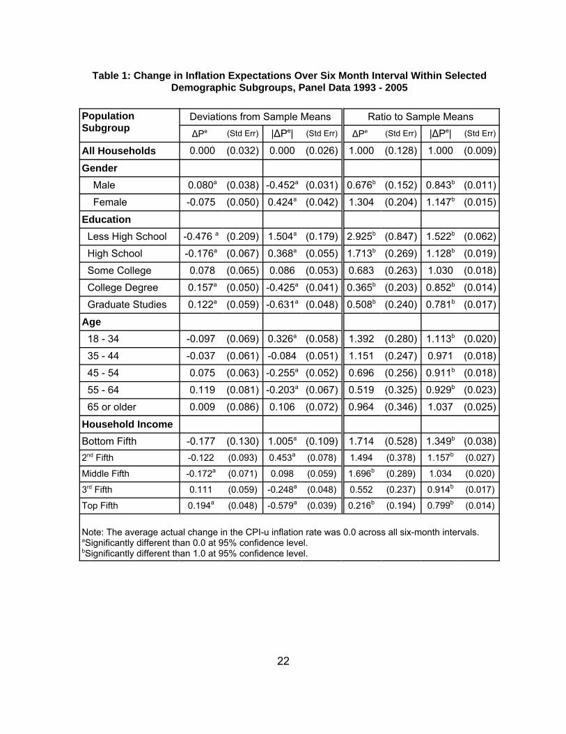
Based on the six-month differences, comparisons were made across selected demographicsubgroups that could be reasonably expected to differ in the costs of updating inflationexpectations. Education was selected given that the formation of inflation expectations is assumedto critically depend on the ability of the respondents to gather and interpret information; gender wasselected since information gathered from personal shopping experience may provide an informationadvantage to women8; age and income were selected since the economic situation andexperiences are likely to differ over the life cycle.
Given the purpose of the analysis is to identify groups with relatively high or lowheterogeneity, the overall sample mean was subtracted, with the analysis focused on the deviationsfrom the mean. Recall that the observed change in inflation expectations was one-quarter of apercentage point, compared with the change in the actual CPI across all six-month intervals of zeroin the 1993 to 2005 period.
A second measure of relative heterogeneity is the ratio of individual differences to thesample difference. Thus, whenever the ratio was above 1.0 for a particular subgroup, it wouldindicate that they had proportionately higher heterogeneity than other members of the panel duringthe same six-month interval. The sample consisted of 26,611 cases that had complete data onboth measures with the interviews conducted from 1993 to 2005.
Consider the results for gender as shown in Table 1. Men raised their inflation expectationsby +0.080 percentage points over the six month interval on average, nearly the exact opposite of
14
the -0.075 decline recorded by women. Recall that the overall sample mean was -0.247, so thatthe positive deviation of +0.080 for men was closer to the average actual change in the CPI of 0.0.The absolute differences were also offsetting, although the average absolute differences weremuch larger: men recorded a smaller than average absolute error of -0.452 and women a largererror of +0.424. The ratio data indicated that the error among men was 67.6% of the average andfor women it was 130.4% of the sample average. The difference was somewhat narrower with theratio of the absolute errors.
The differences by education level conform to the hypothesis that the costs of collecting andprocessing relevant data decline as education increases. In the lowest education subgroup, theaverage change in inflation expectations was 2.9 times as large as the average, while among thehighest education subgroup the change was just about half the average. The effects acrosseducation subgroups was nearly linear and significant, with higher education groups exhibiting lessheterogeneity.
The results by age group indicated that both the youngest and oldest age groups exhibitedgreater heterogeneity in expectations. The results, however, were not as large nor as consistentas those recorded by education. Indeed, none of the average deviations were significant, and onlysome of the absolute deviations proved to be significant. The results by income groups indicatethat the least heterogeneity among the top forty percent of the income distribution, and the largestheterogeneity was among those in the lowest fifth of the income distribution.
Overall, the data provide some support for the hypothesis that the costs involved incollecting and procession information play a role in the decision to update inflation expectations.Among groups that faced higher costs, the level of heterogeneity was greater indicating lessfrequent updating, most notably among the least educated; correspondingly, groups that facedlower costs and higher benefits exhibited more frequent updating and less heterogeneity, moststrongly shown by upper income subgroups.
Staggered Information Flows
Although the two-wave panel data can not rigorously test theories of staggered informationflows, it can provide some guidance. The theory is typically expressed in terms of the delayedresponse in updating expectations. Since the panel includes a measure of only one change inexpectations, an analysis of the timing of the updating of expectations over time is not possible.Instead, the process can conceptualize in reverse: rather than postulating that a given change inthe actual inflation rate has a staggered impact on a series of future changes in expectations, it ispostulated that a given change in inflation expectations resulted from the staggered impact of aseries of past changes in the actual inflation rate.
Past changes in the actual inflation rate were used as predictors in a regression analysisof the change in inflation expectations. For this analysis, the past change in the inflation rate wasdefined as the difference between the monthly change in the CPI (at annual rates) at time t and t-1.Since the measured change in inflation expectations occurred over a six month interval, changesin the actual inflation rate within that six month interval would not unambiguously support thehypothesis of staggered information flows. Changes in the actual inflation rate that occurred morethan six months ago could more reasonably be anticipated to support the hypothesis. As a result
15
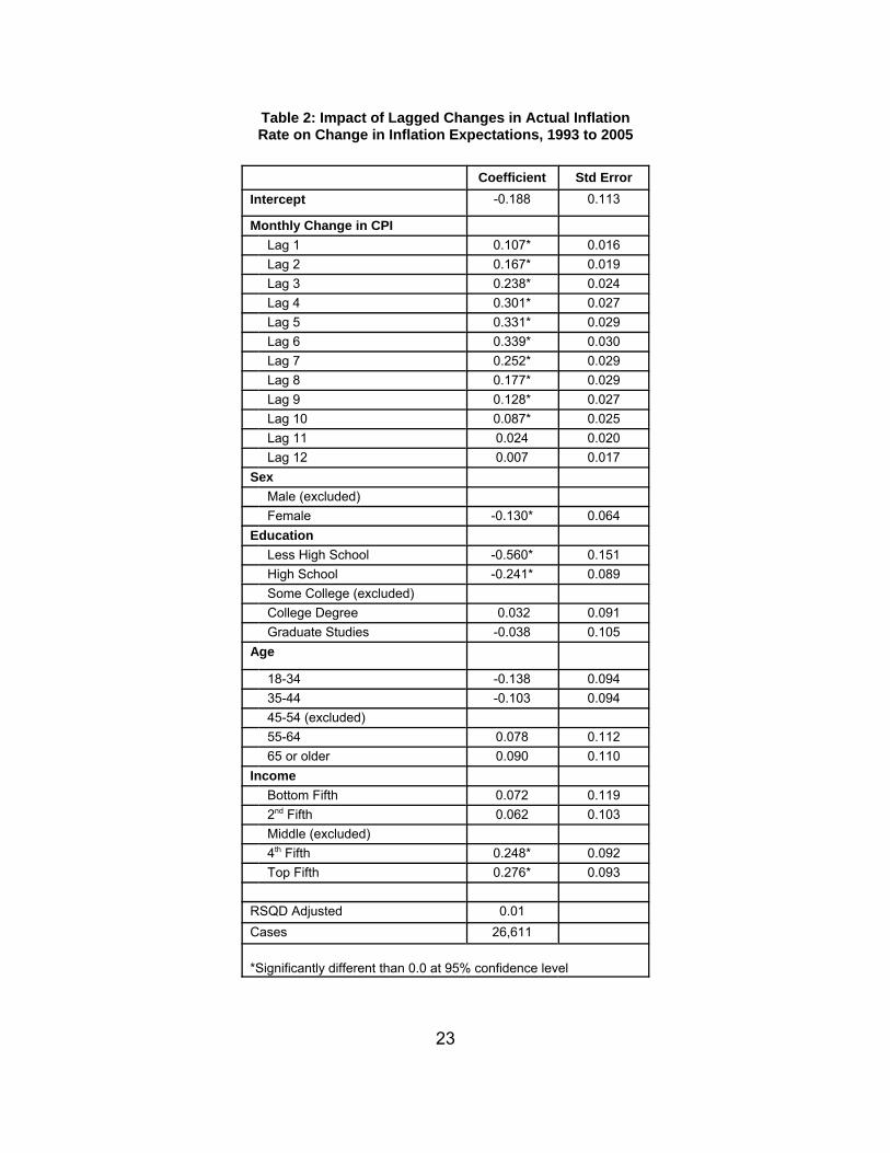
12 lagged changes in the monthly inflation rate were entered into the regression. In addition,dummy variables for the demographic characteristics discussed above were also included.
The results of the regression are shown in Table 2. While the first six lags of the actualchange in the inflation rate were significant contributors to the change in inflation expectations, thiscould simply reflect normal updating not the staggered information hypothesis. Nonetheless, it isworth noting that the pattern in the size of the coefficients: they increase in size from the first lagto the fourth lag and reach a peak at the sixth lag. The significance of the seventh to the tenth lagsoffer greater support for the hypothesis that staggered information flows have a significant impacton expectations. It is of some importance to note that all of these variables combined explainedjust 1% of the total variation in inflation expectations. So even if the data support the staggeredinformation hypothesis, the support is quite meager.
Asymmetric Impact of Information
The hypothesis that unfavorable information about inflation prompts widespread and promptresponses in inflation expectations can be tested by a comparison of positive and negative changesin the actual inflation rate with subsequent changes in expectations. For each six month intervalin the panel, the change in inflation expectations was compared with the change in the actualinflation rate during the prior six months, with negative and positive changes entered separately.The regressions included 26,611 cases from 1993 to 2005.
The estimated results were consistent with the hypothesis that increases in the inflation ratehad a much larger impact than declines on inflation expectations. The coefficient for an increasein inflation was 0.117 (standard error of 0.020), nearly twice the size of the coefficient for declinesin inflation of 0.068 (standard error of 0.020). The estimate that negative news about inflation wastwice as powerful as positive news is consistent with prospect theory (Kahneman and Tversky,1979).
The asymmetrical response of inflation expectations may mean that there is also anasymmetrical response to changes in the perceived credibility of central banks. Increases ininflation will more promptly diminish the credibility of central banks, but declines in inflation will onlyslowly rebuild lost credibility.
Backward or Forward-Looking Expectations?
Tests of whether the formation of inflation expectations represents a backward or forward-looking process have typically been examined in separate equations, with the analyst having theresponsibility to judge the comparative evidence. There is a way to nest both hypotheses in thesame reduced form equation by regressing current inflation expectations on both past and futurechanges in the actual inflation rate. Strong support for the adaptive hypothesis would bedemonstrated if past but not future changes in the actual inflation rate were significant predictors,while support for forward-looking expectations would be shown if future but not past changes in theactual inflation rate were significant predictors. Many will recognize the resulting equation as simplyanother method to test for “Granger causality” (Geweke, Meese and Dent, 1982). The estimatedequation was fitted from 1978 to 2005 was:
1See Lott and Miller (1982), Gramlich (1983), Grant and Thomas (1999), Thomas (1999), Mehra (2002), Roberts (1997),Badhestani (1992), Bryan and Gavin (1986), Noble and Fields (1982), Batchelor and Dua (1989),
2Cukierman (1986) has suggested that this is not a clear violation of the rational expectations hypothesis, since householdsmay not always correctly distinguish between temporary and permanent shocks and thus their forecasts could exhibit seriallycorrelated errors.
3Similar comparisons were done for year-ahead forecasts of the national unemployment rate. Curtin (1999, 2003) found thatconsumers’ forecasts of the year-ahead unemployment rate outperformed those of professional forecasters as well asforecasts from two prominent macroeconomic models.
16
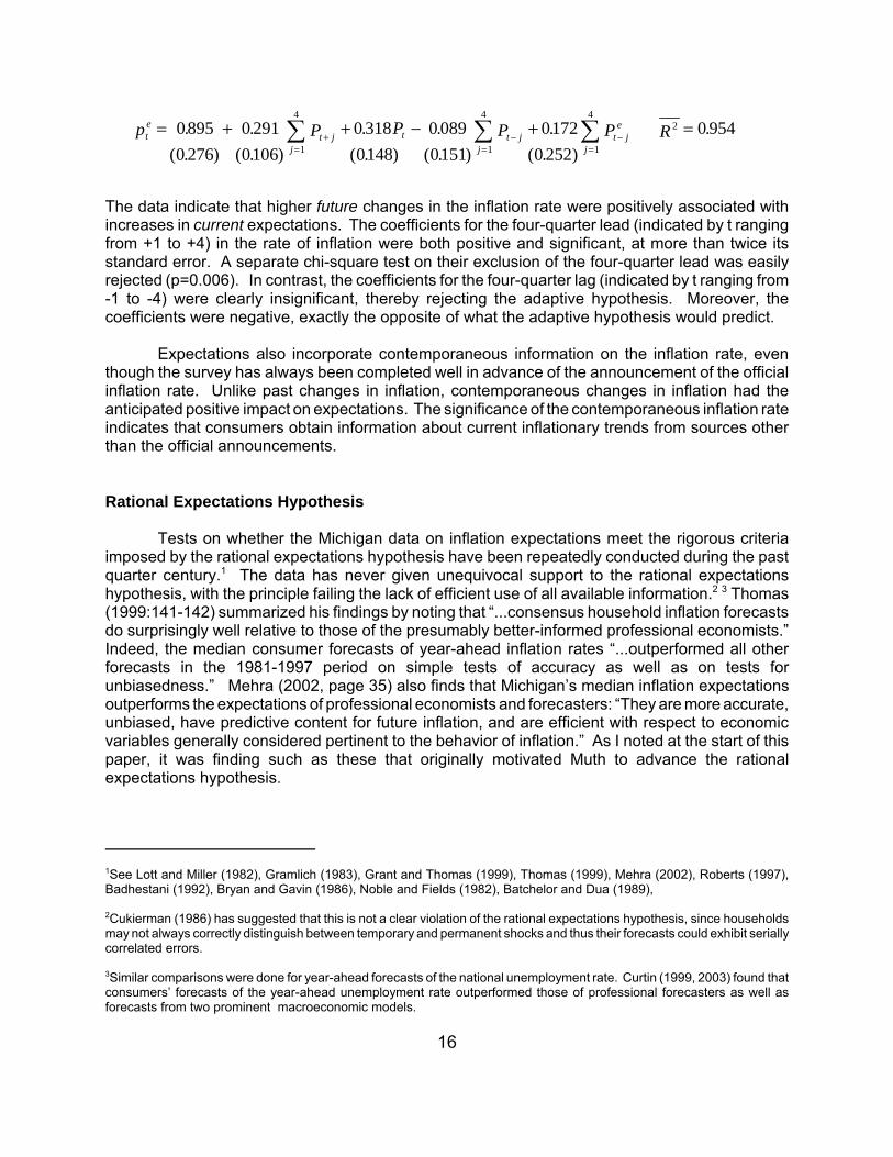
The data indicate that higher future changes in the inflation rate were positively associated withincreases in current expectations. The coefficients for the four-quarter lead (indicated by t rangingfrom +1 to +4) in the rate of inflation were both positive and significant, at more than twice itsstandard error. A separate chi-square test on their exclusion of the four-quarter lead was easilyrejected (p=0.006). In contrast, the coefficients for the four-quarter lag (indicated by t ranging from-1 to -4) were clearly insignificant, thereby rejecting the adaptive hypothesis. Moreover, thecoefficients were negative, exactly the opposite of what the adaptive hypothesis would predict.
Expectations also incorporate contemporaneous information on the inflation rate, eventhough the survey has always been completed well in advance of the announcement of the officialinflation rate. Unlike past changes in inflation, contemporaneous changes in inflation had theanticipated positive impact on expectations. The significance of the contemporaneous inflation rateindicates that consumers obtain information about current inflationary trends from sources otherthan the official announcements.
Rational Expectations Hypothesis
Tests on whether the Michigan data on inflation expectations meet the rigorous criteriaimposed by the rational expectations hypothesis have been repeatedly conducted during the pastquarter century.1 The data has never given unequivocal support to the rational expectationshypothesis, with the principle failing the lack of efficient use of all available information.2 3 Thomas(1999:141-142) summarized his findings by noting that “...consensus household inflation forecastsdo surprisingly well relative to those of the presumably better-informed professional economists.”Indeed, the median consumer forecasts of year-ahead inflation rates “...outperformed all otherforecasts in the 1981-1997 period on simple tests of accuracy as well as on tests forunbiasedness.” Mehra (2002, page 35) also finds that Michigan’s median inflation expectationsoutperforms the expectations of professional economists and forecasters: “They are more accurate,unbiased, have predictive content for future inflation, and are efficient with respect to economicvariables generally considered pertinent to the behavior of inflation.” As I noted at the start of thispaper, it was finding such as these that originally motivated Muth to advance the rationalexpectations hypothesis.
p P P P P Rte
t jj
t t jj
t je
j
= + + − + =+=
−=
−=
∑ ∑ ∑08950 276
0 2910106
0 3180148
0 0890151
01720 252
0 9541
4
1
4
1
42.
( . ).
( . ).
( . ).
( . ).
( . ).
4Insufficient data in the first half of the period made it impossible to code real household income in a consistent fashion andso this variable was excluded from this analysis.
17
What I will focus on is the puzzle that consumers’ performance at forecasting the inflationrate is comparable to forecasts by economists. This finding is more troublesome for those whofavor some form on the adaptation hypothesis, but it is also quite difficult to argue that the costs ofcollecting and processing information is not significantly lower for economists than for consumers.Only under the hypothesis that the costs are trivial would no significant differences betweeneconomists and consumers be anticipated.
Another hypothesis is that the errors in consumer expectations are offsetting, and as aconsequence the test were misleading. Thus, the errors could be quite large, say a significantunderestimate among men is offset by a significant overestimate among women, or similaroffsetting shifts among education or age subgroups. To examine this issue, a number ofregressions were performed for a selection of demographic subgroups. Given that survey datausually involve some aggregation errors, the regression was calculated using nonlinear leastsquares to estimate a moving average error term, using a consistent estimate of the covariancematrix that allows for serial correlation and heteroscedasticity. The overlapping forecast intervalsgenerated by the survey questions could produce serially correlated errors even among perfectlyrational agents (Croushore, 1998). In fact, a significant first order moving average error term wasfound in all equations. The residuals are also tested for the inefficient use of information oninflation, but no tests were attempted for the inefficient use of other relevant information (what iscalled strong efficiency).
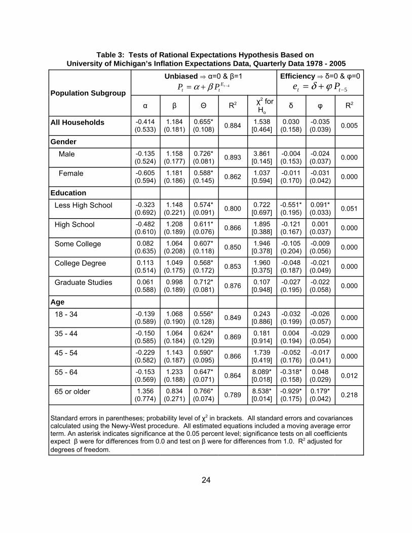
Regressions were estimated for men and women as well as different education and agesubgroups and the results are reported in Table 3. The regressions are based on quarterlyobservations from 1978 to 2005. Given the rather small monthly sample sizes, to insure thatestimates for each subgroup were based on a sufficient number of cases, the independent monthlysamples were pooled into quarterly observations to calculate the median inflation expectations foreach subgroup.4
The results of the analysis indicated that rather than offsetting errors, the year-aheadinflation expectations of each of the demographic groups were an unbiased estimate of the actualinflation rate. The null hypothesis that inflation expectations were a biased estimate was rejectedfor every demographic subgroup at the 95% confidence level: every constant term wasinsignificantly different from zero, and every estimated coefficient on inflation expectations wasinsignificantly different from one. Every equation had a significant estimate of the moving averageerror term, but only among the least educated and the older respondents was there any evidenceof the inefficient use of information about the inflation rate that was available at the time theirexpectations were formed.
These results have always been met with disbelief. Could it be that the costs of formingunbiased inflation expectations are more manageable based on staggered updating? Does thepresumably lower cost and greater importance of private information play a more pivotal role in theformation of expectations than suggested by current theories? Or is the accuracy of expectationsa property of groups and consensus forecasts? Could it be that the rational expectationshypothesis is true at the macro but not at the micro level?
18
Concluding Comments
There are at least as many unresolved issues now as when the rational expectationshypothesis was first advanced nearly a half century ago. Indeed, the findings from this analysis canbe summarized in much the same way as Muth did in his classic article: consumers’ inflationexpectations are forward looking, they are generally as accurate as the forecasts of economicmodels, and they more closely correspond to the hypothesis of rational expectations than to thebackward-looking hypothesis of adaptation.
There is no doubt that people sometimes engage in adaptative behaviors, correct pasterrors, or simply rely on extrapolation to form expectations. These shortcuts are used to helpreduce the costs involved in collecting and processing data. These costs result in staggeredchanges in expectations. In turn, staggered or sticky expectations are the likely cause of the findingthat consumers do not take into account all available information when forming their expectations.It is simply too costly given the expected benefit. These finding, however, do not contradict therational expectations hypothesis but act to incorporate the hypothesis more fully into the standardeconomic framework.
Moreover, the finding that consumers are not fully rational in forming their inflationexpectations is as surprising as the finding that consumers do not fully maximize their utility! Theprofession needs to accept what amounts to a simplifying assumption that is roughly consistent withthe evidence at the macro level. The acceptance should be based on its predictive performance,not on the realism of the theory’s assumptions. To be sure, full rationality is unlikely to be observedin everyday life among consumers nor even among economists. Analysis at the micro level stillneeds to more fully incorporate aspects of bounded rationality and other innovations of behavioraltheory.
Most of the theoretical implication of rationality for monetary policy, however, may be closelyapproximated by “nearly rational” expectations. Without a more exact and universal definition ofwhat “near rationality” means, that glass will be seen as half empty by some and half full by others.It is that unresolved ambiguity that continues to makes monetary policy an interesting andchallenging task.
19
References
Albanesi, Stefania, V.V. Chari, and Lawrence Christiano, “Expectations Traps and Monetary Policy,” NBERworking paper 8912, 2002.
Bacchetta, Philippe and Eric van Wincoop, “Rational Inattention: A Solution to the Forward Discount Puzzle,”Working paper 11633, National Bureau of Economic Research, September 2005.
Baghestani, H., “Survey Evidence on the Muthian Rationality of the Inflation Forecasts of U.S. Consumers,”Oxford Bulletin of Economics and Statistics, vol. 54, pp. 173-186, 1992.
Baker, Michael, “Digit Preferences in CPS Unemployment Data,” Economic Letters, vol. 39, issue 1, pp. 117-121, 1992.
Batchelor, R., “Quantitative versus Qualitative Measures of Inflation Expectations,” Oxford Bulletin ofEconomics and Statistics, vol 48, no 2, 99-120, 1986.
Batchelor, R. A. and Pami Dua, “Household versus Economists Forecasts of Inflation: A reassessment,”Journal of Money, Credit, and Banking, vol. 21, pp. 252-257, 1989.
Begg, David K.H., The Rational Expectations Revolution in Macroeconomics, John Hopkins University Press,1982.
Branch, William A., “Sticky Information and Model Uncertainty in Survey Data on Inflation Expectations,”mimeo, July 2005.
Bryan, Michael and Guhan Venkatu, “The Curiously Different Inflation Perspectives of Men and Women,”Federal Reserve Bank of Cleveland, Economic Commentary Series, 2001.
Bryan, Michael and Stefan Palmqvist, “Testing Near-Rationality using Detailed Survey Data,” Economic Paper228, European Commission, Economic and Financial Affairs, July 2005.
Bryan, M. F. and W. T. Gavin, “Models of Inflation Expectations Formation: A Comparison of Household andEconomist Forecasts,” Journal of Money, Credit, and Banking, vol. 18 (4) pp. 539-44, 1986.
Breusch, T. S., “Testing for Autocorrelation in Dynamic Linear Models,” Australian Economic Papers, vol 17,334-355, 1978.
Cagan, Phillip, “The Monetary Dynamics of Hyperinflation,” in Milton Friedman, ed., Studies in the QuantityTheory of Money, 25-117, University of Chicago Press, Chicago, 1956.
Carlson, J., and M. Parkin, “Inflation Expectations,” Economica, vol 42, 123-138, 1975.Carroll, Christopher, “Macroeconomic Expectations of Households and Professional Forecasters,” Quarterly
Journal of Economics, vol. 118 (1), pp. 269-298, 2003.Chari, V.V., Lawrence Christiano, and Martin Eichenbaum, “Expectation Traps and Discretion,” Journal of
Economic Theory, vol. 2, pp. 462-92, 1998.Croushore, Dean, “Evaluating Inflation Expectations,” Working Paper No. 98-14, Federal Reserve Bank of
Philadelphia, 1998.Croushore, Dean, and Tom Stark, “Real Time Data Sets for Macroeconomists: Does the Data Vintage
Matter?” Working paper 21, Federal Reserve Bank of Richmond, 1999.Cukierman, Alex, “Measuring Inflationary Expectations,” Journal of Monetary Economics, vol 17, 315-324,
1986.Curtin, Richard, “Unemployment Expectations: The Impact of Private Information on Income Uncertainty,”
Review of Income and Wealth, vol. 49, no. 4, 2003.Curtin, Richard, “What Recession? What Recovery? The Arrival of the 21st Century Consumer,” Business
Economics, vol. 39, no. 2, 2003.Curtin, Richard, “The Outlook for Consumption in 2000,” The Economic Outlook for 2000, Ann
Arbor, Michigan: University of Michigan, 1999.Doms, Mark and Norman Morin, “Consumer Sentiment, the Economy, and the News Media,” working paper
2004-51, Federal Reserve Board, 2004.Edouard, L and A. Senthilselvan, “Observer Error and Birthweight: Digit Preference in Recording,” Public
Health, vol. 111 (2), pp. 77-79, 1997.Earl, P. E. , Economics and psychology: A survey. Economic Journal, 100(402), 718-755, 1990.Evans, George W. and Seppo Honkapohja, Learning and Expectations in Macroeconomics, Princeton
University Press: 2001.
20
Figlewski, Stephen and Paul Wachtel, “Rational Expectations, Informational Efficiency, and Tests UsingSurvey Data: A Reply,” Review of Economics and Statistics, vol 65, pp 529-531.
Friedman, Milton, Essays in Positive Economics. M. Friedman Essays in Positive Economics . Chicago:University of Chicago Press, 1953.
Gerberding, Christina, “The Information Content of Survey Data on Expected Price Developments forMonetary Policy,” Discussion Paper 9/01, Deutsche Bundesbank, April 2001.
Geweke, J., R. Meese, and W. Dent, “Comparing Alternative Tests of Causality in Temporal Systems,”Journal of Econometrics, vol 21, no 2, 161-194, February 1983.
Grant, Alan P. and Lloyd B. Thomas, “Inflationary Expectations and Rationality Revisited,” Economic Letters,vol. 62 (March), pp. 331-338, 1999.
Gramlich, Edward M., “Models of Inflation Expectations Formation,” Journal of Money, Credit, and Banking,vol. 15, pp 155-73, 1983.
Hamilton, James, All the News That’s Fit to Sell, Princeton University Press, 2004.Kahneman, Daniel, and AmosTversky, “Prospect Theory: An Analysis of Decision Under Risk,”
Econometrica, vol. 47, no. 2, pp. 263-292, 1979.Kean, Michael and David Runkle, “Testing the Rationality of Price Forecasts: New Evidence from Panel
Data,” American Economic Review, vol 80 (September), pp.714-735Kean, Michael P. and David E. Runkle, “Are Economic Forecasts Rational,” Federal Reserve Bank of
Minneapolis Quarterly Review, Spring 1989, pp. 26-33.Khan, Hashmat and Zhenhua Zhu, “Estimates of Sticky Information Phillips Curve for the United States,
Canada, and the United Kingdom,” Working paper 2002-19, Bank of Canada, 2002.Koyck, Leendert Marinus, Distributed Lags and Investment Analysis, North-Holland, Amsterdam, 1954.Leduc, Sylvain, Keith Sill, and Tom Stark, “Self-Fulfilling Expectations and the Inflation of the 1970's:
Evidence from the Livingston Survey,” Wording paper 02-13R, Federal Reserve Bank ofPhiladelphia, May 2003.
Mankiw, N. Gregory, Ricardo Reis, and Justin Wolfers, “Disagreement about Inflation Expectations,”Macroeconomics Annual 2003, eds. Mark Gertler and Kenneth Rogoff, NBER: 2004.
Mankiw, N. Gregory and Ricardo Reis, “Sticky Information Versus Sticky Prices: A proposal to Replace theNew Keynesian Phillips Curve,” Quarterly Journal of Economics, vol. 117 (4), pp. 1295-1328.
Mankiw, N. Gregory and Ricardo Reis, “Sticky Information: A Model of Monetary Non-neutrality andStructural Slumps,” in P. Aghion, R. Frydman, J. Stiglitz and M. Woodford, eds., Knowledge,Information and Expectations in Modern Macroeconomics: In Honor of Edmund S. Phelps,Princeton University Press, 2003.
Mehra, Yash P., “Survey Measures of Expected Inflation: Revisiting the Issues of Predictive Content andRationality,” Federal Reserve Bank of Richmond Economic Quarterly, vol. 88 (3), pp. 17-36, 2002.
Muth, John F., “Rational Expectations and the Theory of Price Movements,” Econometrica, vol 29, no 3,315-335, July 1961.
Nerlove, Marc, “Adaptive Expectations and Cobweb Phenomena,” Quarterly Journal of Economics, vol 72,no 2, 227-240, May 1958.
Noble, Nicholas R. and T. Windsor Fields, “Testing the Rationality of Inflation Expectations Derived fromSurvey Data: A Structure-Based Approach,” Southern Economic Journal, vol. 49 (2) pp. 361-373,1982.
Pesaran, M. H. The Limits of Rational Expectations, Basil-Backwell, Oxford, 1987.Rabin, M., Psychology and economics. Journal of Economic Literature, XXXVI, 11-46, 1998.Rabin, M., & Schrag, J. L., First Impressions Matter: A Model of Confirmatory Bias. Quarterly Journal of
Economics, 114(1), 37-82, 1999.Roberts, John M., “Is inflation Sticky,” Journal of Monetary Economics, vol. 39, pp. 173-196, 1997.Sims, Christopher, “Implications of Rational Inattention,” Journal of Monetary Economics, vol. 50 (3), pp.
665-690.Souleles, Nicholas S., “Consumer Sentiment: Its Rationality and Usefulness in Forecasting
Expenditures—Evidence from the Michigan Micro Data,” Journal of Money, Credit, and Banking,forthcoming.
Thaler, R. H., Quasi-Rational Economics. R. H. Thaler Quasi-Rational Economics . New York: RussellSage Foundation, 1991.
21
Thaler, R. H. , The Winner's Curse. R. H. Thaler The Winner's Curse . Princeton: Princeton UniversityPress, 1992.
Thomas Jr., Lloyd B., “Survey Measures of Expected U.S. Inflation,” Journal of Economic Perspectives,vol 13, no 4, 125-144, Autumn 1999.
Tversky, A., & Kahneman, D. , Causal schemas in judgements under uncertainty. D. Kahneman, P. Slovic,& A. Tversky (Editors), Judgment under uncertainty: Heuristics and biases (pp. 117-128).Cambridge: Cambridge University Press, 1982.
Woodford, Michael, Interest and Prices: Foundations of a Theory of Monetary Policy, Princeton UniversityPress, 2003.
Woodford, Michael, “Robustly Optimal Monetary Policy with Near Rational Expectations,” NBER workingpaper 11896, 2005.
Zarnowitz, Victor, “Rational Expectations and Macroeconomic Forecasts,” Journal of Business andEconomic Statistics, vol. 3(October), pp. 293-311, 1985.
22
Table 1: Change in Inflation Expectations Over Six Month Interval Within SelectedDemographic Subgroups, Panel Data 1993 - 2005
PopulationSubgroup
Deviations from Sample Means Ratio to Sample Means∆Pe (Std Err) |∆Pe| (Std Err) ∆Pe (Std Err) |∆Pe| (Std Err)
All Households 0.000 (0.032) 0.000 (0.026) 1.000 (0.128) 1.000 (0.009)
Gender Male 0.080a (0.038) -0.452a (0.031) 0.676b (0.152) 0.843b (0.011)
Top Fifth 0.194a (0.048) -0.579a (0.039) 0.216b (0.194) 0.799b (0.014)
Note: The average actual change in the CPI-u inflation rate was 0.0 across all six-month intervals.aSignificantly different than 0.0 at 95% confidence level.bSignificantly different than 1.0 at 95% confidence level.
23
Table 2: Impact of Lagged Changes in Actual InflationRate on Change in Inflation Expectations, 1993 to 2005
*Significantly different than 0.0 at 95% confidence level
24
Table 3: Tests of Rational Expectations Hypothesis Based on University of Michigan’s Inflation Expectations Data, Quarterly Data 1978 - 2005
Population Subgroup
Unbiased | α=0 & β=1P Pt t
Et= + −α β 4
Efficiency | δ=0 & φ=0e Pt t= + −δ ϕ 5
α β Θ R2 χ2 forHo
δ φ R2
All Households -0.414(0.533)
1.184(0.181)
0.655*(0.108) 0.884 1.538
[0.464]0.030
(0.158)-0.035(0.039) 0.005
Gender Male -0.135
(0.524)1.158
(0.177)0.726*(0.081) 0.893 3.861
[0.145]-0.004(0.153)
-0.024(0.037) 0.000
Female -0.605(0.594)
1.181(0.186)
0.588*(0.145) 0.862 1.037
[0.594]-0.011(0.170)
-0.031(0.042) 0.000
Education Less High School -0.323
(0.692)1.148
(0.221)0.574*(0.091) 0.800 0.722
[0.697]-0.551*(0.195)
0.091*(0.033) 0.051
High School -0.482(0.610)
1.208(0.189)
0.611*(0.076) 0.866 1.895
[0.388]-0.121(0.167)
0.001(0.037) 0.000
Some College 0.082(0.635)
1.064(0.208)
0.607*(0.118) 0.850 1.946
[0.378]-0.105(0.204)
-0.009(0.056) 0.000
College Degree 0.113(0.514)
1.049(0.175)
0.568*(0.172) 0.853 1.960
[0.375]-0.048(0.187)
-0.021(0.049) 0.000
Graduate Studies 0.061(0.588)
0.998(0.189)
0.712*(0.081) 0.876 0.107
[0.948]-0.027(0.195)
-0.022(0.058) 0.000
Age 18 - 34 -0.139
(0.589)1.068
(0.190)0.556*(0.128) 0.849 0.243
[0.886]-0.032(0.199)
-0.026(0.057) 0.000
35 - 44 -0.150(0.585)
1.064(0.184)
0.624*(0.129) 0.869 0.181
[0.914]0.004
(0.194)-0.029(0.054) 0.000
45 - 54 -0.229(0.582)
1.143(0.187)
0.590*(0.095) 0.866 1.739
[0.419]-0.052(0.176)
-0.017(0.041) 0.000
55 - 64 -0.153(0.569)
1.233(0.188)
0.647*(0.071) 0.864 8.089*
[0.018]-0.318*(0.158)
0.048(0.029) 0.012
65 or older 1.356(0.774)
0.834(0.271)
0.766*(0.074) 0.789 8.538*
[0.014]-0.929*(0.175)
0.179*(0.042) 0.218
Standard errors in parentheses; probability level of χ2 in brackets. All standard errors and covariancescalculated using the Newy-West procedure. All estimated equations included a moving average errorterm. An asterisk indicates significance at the 0.05 percent level; significance tests on all coefficientsexpect β were for differences from 0.0 and test on β were for differences from 1.0. R2 adjusted fordegrees of freedom.
25
Chart 1: Year-Ahead Inflation Expectations:Distribution of Responses, 1978 – 2004