Corporate Bond Market Transparency and Transaction Costs*

Amy K. Edwards**, Lawrence E. Harris, Michael S. Piwowar

Original Draft: October 2004 Current Draft: March 2005 *The paper has benefited from the comments of Chester Spatt, Lisa Hasday, Yolanda Goettsch, Bruno Biais, Pam Moulton, Gideon Saar, and seminar participants at the Securities and Exchange Commission, the University of Delaware, George Washington University, the Utah Winter Finance Conference, Barclays Global Investors, the Bank of Canada, Arizona State University, Emory University, and the Institute for Quantitative Analysis in Finance Research. Amy Edwards and Mike Piwowar are financial economists in the Office of Economic Analysis of the U.S. Securities and Exchange Commission. Larry Harris is the Fred V. Keenan Chair in Finance at the University of Southern California. Much of the work was completed while Dr. Harris was Chief Economist at the Securities and Exchange Commission. The Securities and Exchange Commission disclaims responsibility for any private publication or statement of any SEC employee. This study expresses the authors’ views and does not necessarily reflect those of the Commission, the Commissioners, or other members of the staff. All errors and omissions are the sole responsibility of the authors. **Corresponding author. U.S. Securities and Exchange Commission, Office of Economic Analysis, 450 Fifth Street, NW, Washington, DC 20549-1105, USA; Phone: 202-551-6663; Fax: 202-942-9657; Email: edwardsa@sec.gov.

Corporate Bond Market Transparency and Transaction Costs

Abstract

This study examines the effect of the recent introduction of transaction price transparency to the OTC secondary corporate bond market. Using a complete record of all US OTC secondary trades in corporate bonds, we estimate average transaction cost as a function of trade size for each bond that traded more than nine times in 2003. Costs are lower for bonds with transparent trade prices, and they drop when the TRACE system starts to publicly disseminate their prices. The results suggest that public traders will significantly benefit from the additional price transparency. JEL Classification: G10; G20 Keywords: Corporate bonds; fixed income; liquidity; transaction cost measurement; effective

spreads; TRACE; price transparency; market microstructure; dealers.

Secondary trading costs in the corporate bond markets are not widely known outside of the

community of professional fixed income traders. Given the importance of bond financing in our

economy—the aggregate values of corporate bonds and equities are roughly equal in the US—it

is somewhat surprising that so little is known about the costs of trading bonds. This study

characterizes these costs using a record of every corporate bond trade reported in 2003.

Bond trading costs are not well known because corporate bond markets are not nearly as

transparent as are equity markets. Dealers provide public quotes for few bonds on a continuous

basis, and until recently, most bond transaction prices have never been published. We study

whether this lack of price transparency contributes to bond transaction costs, which we find to be

substantially higher than equity transaction costs.

Our results have implications for investors, issuers, and regulators. Investors incorporate

transactions costs into their portfolio decisions. Their investment decisions depend on the costs

of investing in bonds as well as the costs of divesting from them should they require liquidity

before their bonds mature. Issuers consider secondary market transactions costs when deciding

how to structure their bonds. Bond features that reduce liquidity are unattractive to investors and

therefore costly to issuers.1 Regulators study transaction costs to determine how they depend on

market structure, and in particular, on price transparency. Understanding such relations allows

them to adopt regulatory polices to better promote competition and efficiency.

US bond markets are becoming increasingly transparent. The National Association of

Securities Dealers (NASD) now requires dealers to report all OTC bond transactions through its

TRACE (Trade Reporting and Compliance Engine) bond price reporting system. This system

became operational on July 1, 2002. Under pressure from Congress, buy-side traders and the

1 Amihud and Mendelson (1991) find that bond liquidity influences yield to maturity and, therefore, issuers cost of capital.

1

SEC, the NASD is phasing-in real time dissemination of these prices to the public. As of the end

of 2003, The TRACE system disseminates bond prices no later than 45 minutes after trades

occur in about one-half of all traded bond issues. The Bond Market Association, the trade

organization for bond dealers, questions whether all bonds should be transparent, citing concerns

that transparency will hurt liquidity.2 The results of this study should help inform the debate

over the effect of transparency on liquidity. We find that trading costs are lower for transparent

bonds than for similar opaque bonds, and that these costs fall when a bond’s prices are made

transparent. We interpret these results as evidence that transparency has improved liquidity in

corporate bond markets.

Our cross-sectional and time-series estimates suggest that transparency decreases

customer transaction costs by roughly five basis points and probably more. Our data shows that

in 2003, public investors traded approximately two trillion dollars in bond issues for which

prices were not published on a contemporaneous basis. These results suggest that investors may

save a minimum of one billion dollars per year if the prices of all bonds were made TRACE-

transparent with the existing 45-minute reporting protocol. This figure represents a lower bound

on the cost savings for a couple of reasons.

First, in a related study, Bessembinder, Maxwell, and Venkataraman (2005) find an

immediate reduction in transaction costs at the initiation of the TRACE system in July 2002 for a

group of relatively sophisticated institutional traders (insurance companies). We do not capture

this immediate reduction in trading costs in our analysis, which Bessembinder, Maxwell, and

Venkataraman (2005) estimate to be roughly $370 million per year for this institutional segment

of the market.

2 See, for example, “Testimony before The Committee on Banking, Housing and Urban Affairs, United States Senate,” Statement of Micah S. Green, President, The Bond Market Association, June 17, 2004 Oversight Hearing

2

Second, learning how to obtain, organize, and use price data takes time for less

sophisticated traders. For example, most retail traders and many institutional traders now do

not—indeed cannot—obtain last trade prices from their brokers at the time they submit their

orders. Accordingly, we will not observe the full effect of transparency on transaction costs

immediately after prices have been made more transparent. Since our cost savings estimate is

based on information about transaction costs that was collected while traders were still learning

about the availability of price data, we undoubtedly have underestimated the ultimate total cost

savings.

The discussion proceeds as follows. Section I reviews the related literature. Section II

describes our data and sample selection procedures and presents final sample characteristics.

Section III describes the methods we use to estimate average bond transaction costs. Sections IV

and V respectively present time-series and cross-sectional results based on these methods.

Section VI introduces the method we use to estimate time varying transaction costs for a set of

bonds and shows that transaction costs substantially dropped in bonds that became TRACE-

transparent during our sample period. Finally, Section VII concludes and discusses the

importance of the results in the context of current regulatory initiatives.

I. Related Literature

The academic literature considers price transparency to be an important determinant of

the liquidity of securities. For example, see O’Hara (1997) and Madhavan (2000) for a survey.

The previous literature on transparency yields mixed predictions on the effect of changes in

transparency on transaction costs (See Biais, Glosten, and Spatt (2005)). The public debate on

transparency in bond markets is just as divided. Some argue that introducing price transparency

to the bond markets will facilitate better deterrence and detection of fraud and manipulation and

on Bond Market Regulation.

3

will improve pricing efficiency and competition in bond markets, which will lead to lower

transaction costs.3 Others contend that transparency will increase dealers’ costs of providing

liquidity, which will lead to less dealer participation, less competition, less liquidity, and

ultimately higher transaction costs.4 This study is the first to comprehensively and directly

examine how introducing price transparency affects corporate bond transaction costs. With the

exception of an experimental study (see Bloomfield and O’Hara, 1999), we are not aware of any

study examining the introduction of price transparency to other secondary financial markets.5

Therefore, this analysis is an important contribution to the broader understanding of transparency

choices.

Our study uses the most comprehensive source of transaction data for corporate bond

transactions in the United States. We use transaction data from the NASD’s TRACE system.

The TRACE data consist of all over-the-counter (OTC) transactions in all corporate bonds.

Other researchers have studied datasets that only include transactions made by some large buy-

side institutions (e.g., Capital Access International) or transactions for a subset of bonds (e.g.,

Fixed Income Pricing System).6

3 See, for example, “Testimony before The United States Senate Committee on Banking, Housing and Urban Affairs,” Statement of Annette Nazareth, Director of the Division of Market Regulation, U.S. Securities and Exchange Commission, June 17, 2004 and the letter on bond market transparency from SEC Chairman Richard Breeden to Senator Donald Riegle dated September 6, 1991. 4 See, for example, “Testimony before The Committee on Banking, Housing and Urban Affairs, United States Senate,” Statement of Micah S. Green, President, The Bond Market Association, June 17, 2004 Oversight Hearing and the letter on bond market transparency from SEC Chairman Richard Breeden to Senator Donald Riegle dated September 6, 1991. 5 Indeed, the opaque setting in the Bloomfield and O’Hara (1999) experiment is not perfectly comparable to the opaque setting in the corporate bond markets. 6 The Capital Access International (CAI), Fixed Income Securities Database (FISD), Datastream, NYSE Automated Bond System (ABS), and other voluntary or limited proprietary datasets tend to contain only a subset of the pricing information useful for many research questions. The CAI dataset, for example, contains only institutional trades that do not represent the full market very well. CAI transactions have a median trade size of $1.5 million (Schultz, 2001) to $4.4 million (Chakravarty and Sarkar, 2003) but we now know from the TRACE data that typical trade sizes in corporate bonds are actually around $30,000. Therefore, while the CAI dataset may prove quite useful for some research questions, it does not capture the overall market very well. Likewise, data from the Fixed Income Pricing System (FIPS) contains complete pricing information when combined with exchange transactions, but this

4

Our study applies and extends the Harris and Piwowar (2005) transaction cost estimation

methods, developed for their study of secondary trading costs of municipal bonds, to corporate

bonds. Their econometric time-series transaction cost model is appropriate for the OTC

corporate bond market because it shares many of the same features with the municipal bond

market: corporate bond dealers do not post firm bid and ask quotes; corporate bond transaction

data include an indicator of whether the trade was a dealer sale to a customer, a dealer purchase

from a customer, or an interdealer transaction; and many corporate bond issues trade very

infrequently. We extend their methods by allowing liquidity to be time varying. This extension

allows us to examine how the introduction of price transparency affects corporate bond

transaction costs.7

Our transaction cost estimation methods differ significantly from those used in earlier

studies of corporate bond trading costs. Previous studies of corporate bond transaction costs

have employed two main approaches. The first approach, used by Hong and Warga (2000),

Chakravarty and Sarkar (2003) and others, computes same-bond-same-day effective spreads.8

This approach compares the average price of buy transactions to sell transactions on the same

day. The requirement of at least one buy and one sell on the same day is extremely limiting in

corporate bonds, because the median number of trades per day is less than one. This approach

eliminates most transactions when estimating bond transaction costs for most bonds, and it

cannot estimate transaction costs for many infrequently traded bonds. This type of estimator

information is available for only a small set of bonds. This limitation means that FIPS does not allow for broad cross-sectional analyses. 7 Harris and Piwowar (2004) could not directly test the effects of price transparency on liquidity in the municipal bond market because bond prices during their sample period were published in this market only if the bond traded four or more times. As a result, they could not disentangle transparency effects from trading activity effects. 8 See also Green, Hollifield, and Schürhoff (2004) and Kalimpalli and Warga (2002).

5

thus is not well suited for inactively traded securities, and therefore, for use in broad cross-

sectional analyses.

The second approach is a regression-based methodology. Schultz (2001) compares each

transaction price to a benchmark price and regresses the difference on a buy/sell indicator. The

coefficient on the buy/sell indicator estimates the transaction costs. His regression approach

offers an improvement over the same-bond-same-day effective spread because it can measure

transaction costs for inactive bonds as well as active bonds. However, Schultz (2001) admits

that this method does not work particularly well for high-yield bonds because the benchmark is

more difficult to estimate. Bessembinder, Maxwell, and Venkataraman (2005) estimate a

variation of the Schultz (2001) model that incorporates company specific information, which

allows them to estimate transaction costs for high-yield bonds.

Chen, Lesmond, and Wei (2002) propose a different regression approach by extending

Lesmond, Ogden, and Trzcinka (1999). Their approach assumes that a zero return day (or a non-

trading day) is observed when the true price changes by less than the transaction costs. Using

this assumption and applying a two-factor return-generating model, Chen, Lesmond, and Wei

(2002) estimate transaction costs.9 Unlike the Schultz (2001) regression approach, their

regression approach uses only end-of-day transaction prices and no buy-sell indicators. Because

many corporate bonds are inactive, observed end of day prices may represent trades early in the

day. Further, a non-trading day in corporate bonds may not necessarily reflect transaction costs

because corporate bonds tend to have close substitutes, and because many bonds are so

infrequently traded that on most days nobody even considers trading them.10

9 As factors, Chen, Lesmond, and Wei (2002) use changes in the interest rate, which are important for investment grade bonds, and returns on the S&P 500 index, which are important for high-yield bonds. 10 These two problems are exaggerated in the Chen, Lesmond, and Wei (2002) estimation because the data they study contains only transactions reported by one large bond dealer. Because the Chen, Lesmond, and Wei (2002)

6

Our transparency and cross-sectional analyses are related to other work in bond market

microstructure. We show that transparent bonds have lower transaction costs than

nontransparent bonds, and that transaction costs drop when bonds become price transparent.

These results are complementary to Alexander, Edwards, and Ferri (2000), who find that

transparent high yield bonds can be fairly liquid, and to Bessembinder, Maxwell, and

Venkataraman (2005), who find declines in transaction costs for insurance company transactions

in corporate bonds around the July 2002 introduction of TRACE.

We examine the effect of credit risk on the corporate bond transaction costs. Previous

studies have examined the effect of credit risk on volume, yield, volatility, and spread but the

results are mixed. For investment grade corporate bonds, Chakravarty and Sarkar (2003) and

Hong and Warga (2000) find that same-bond-same-day spreads increase with credit risk, but

Schultz (2001) finds no liquidity pattern associated with credit risk. Alexander, Edwards, and

Ferri (2000) finds that high-yield bonds with more credit risk have higher trading volume than

high-yield bonds with lower credit risk. Chen, Lesmond, and Wei (2002) examine credit risk

across both high-yield and investment grade corporate bonds, but their results are mixed at best.

For municipal bonds, Downing and Zhang (2004) find increases in volatility with more credit

risk and Harris and Piwowar (2005) find that bonds with higher credit risk are more expensive to

trade. We find that secondary corporate bond transaction costs increase with credit risk.

II. Data and Sample

We obtain reports of every corporate bond trade reported to TRACE for 2003 (252

trading days) from the NASD. Our TRACE data set contains reports of all OTC trades in all

sample period occurs before bond market transparency, the large bond dealer could only have observed a subset of trades. Therefore, the end-of-day prices are more likely to occur early in the day and the observed zero-return days may not really be zero-return days.

7

corporate bonds.11 Data items include the price, time, and size of the transaction as well as the

side (or sides for interdealer transactions) on which the dealer participated. We also have issuer

and issue information provided by TRACE master files in the form of five snapshots taken

during the sample period.

The only trades omitted from TRACE are those that occurred on exchanges, of which the

vast majority occur on in the NYSE’s Automated Bond System (ABS). Fewer than five percent

of all bonds are listed on the NYSE. For those bonds, ABS trades, which are almost all small

retail trades, represent from zero to 40 percent of all transactions. The TRACE dataset thus is

very nearly a complete record of all corporate bond trades.

The NASD started collecting the TRACE dataset on July 1, 2002. Our analysis uses

2003 data to allow market participants to familiarize themselves with the system.

The 2003 TRACE data identifies almost 70,000 securities in which dealers must report

their trades. Dealers made 8.7 million trade reports representing total volume of 9.4 trillion

dollars in only 22,453 of these securities. The remainder of these securities did not trade in

2003. The TRACE master files classify the majority of these bonds as “inactive” issues.

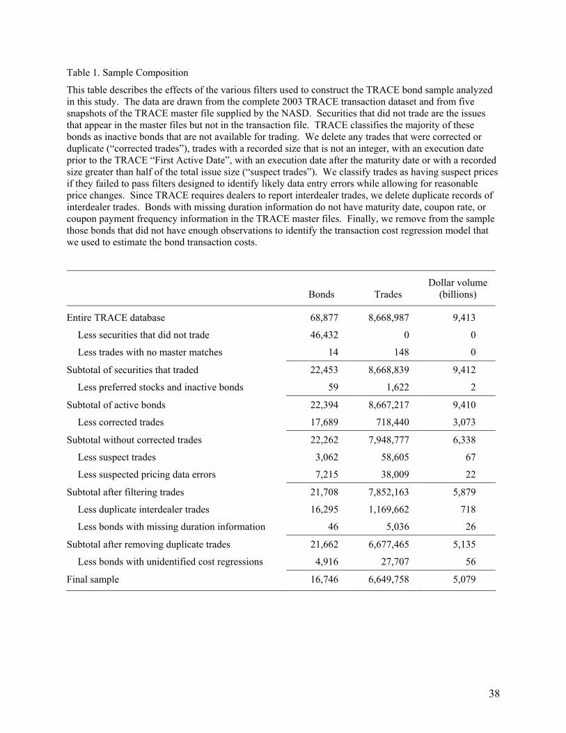
We analyze all trade reports except those that subsequently were corrected, those for

which we suspect the data were incorrectly reported,12 those for which data are missing, those in

11 Note that our data set contains all trades reported to TRACE, whether transparent or not. 12 Filtering for data errors in corporate bonds is somewhat more difficult than in equities because prices for many bonds are observed so infrequently. A large price change filter thus may identify situations where prices changed substantially between transactions that occurred weeks apart. To avoid this problem, we designed two types of filters that operated on deviations from median prices and price reversals. In particular, we first applied the median filter. Because corporate bond prices can change drastically with new company information, we first examined the bonds that did not seem to experience the large price changes and deleted any trades with prices that deviate from the daily median by more than 10%. For the bonds that did experience price changes, we deleted any trades with prices that deviate more than 10% from a nine-trading-day median centered on the trading date. These median filters eliminate the most obvious pricing errors. Next, we estimate the percentage differences between the transaction price and last transaction price and between the transaction price and the next transaction price. We delete a transaction if the transaction price is different from the lead, lag, and average lead/lag by at least 10%. Because dealers may make the same clerical error more than once, we next estimate dealer prices by averaging the prices of consecutive trades by the same dealer. As with the transaction prices, we find the percentage difference

8

bonds for which the total number of trades reported is insufficient to identify the regression

model that we use to estimate transaction costs,13 and duplicate interdealer trade reports. The

final sample includes 6,649,758 trades in 16,746 bonds representing 5.0 trillion dollars of

volume. The reductions in total trades, total volume and numbers of bonds are respectively due

mostly to duplicate interdealer reports, corrected trades, and unidentified regressions. Table 1

provides a complete breakdown of the effects of these filters on the final sample.

The median issuer in the sample only has two bond issues outstanding. This distribution,

like most cross-sectional distributions, is skewed to the right: The average number of issues

outstanding per issuer is more than seven. The average original issue size is $236 million and

the average issuer has about $1.7 billion total outstanding. Bonds had an average of 12.1 years

to maturity at issuance and have been around for 3.5 years on average. The average coupon in

the sample is 6.3% and the average bond price in the sample is 100.4% of par.

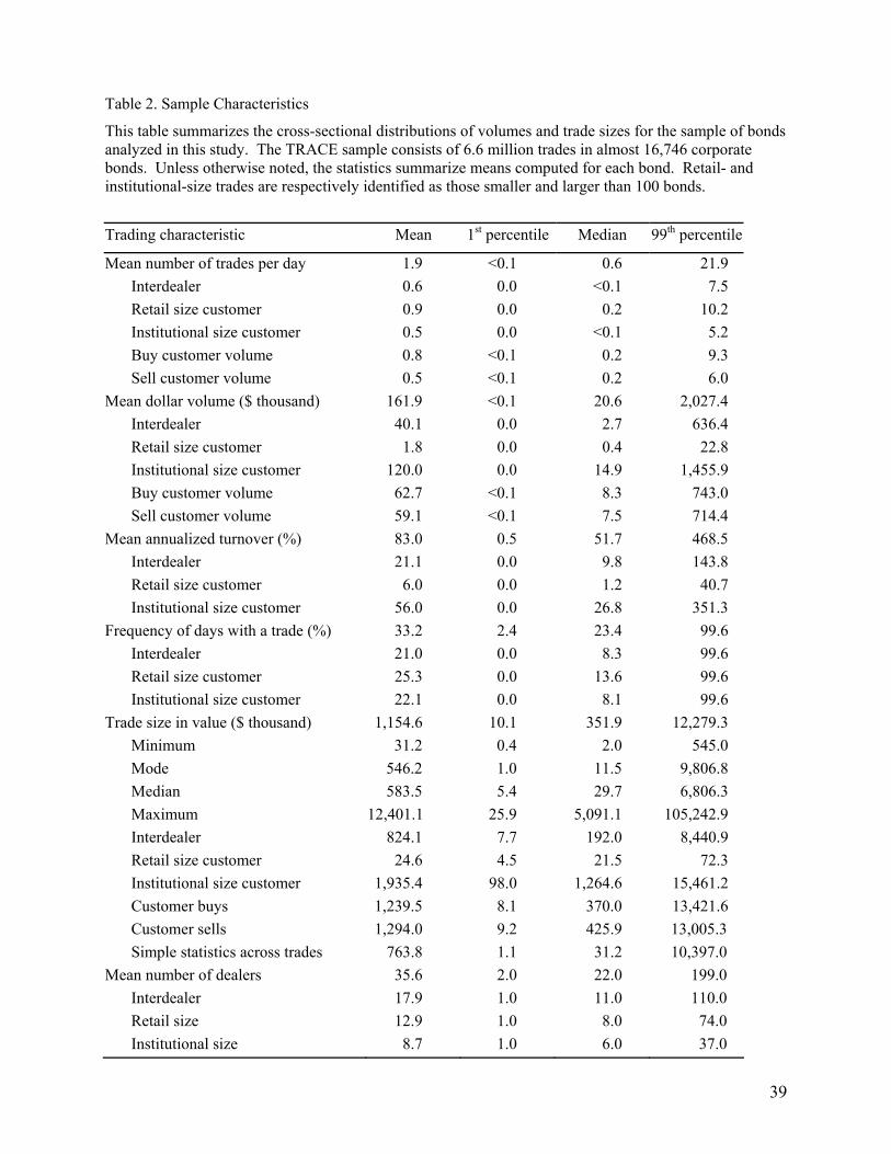
Table 2 provides additional descriptive statistics for our sample. On average, bonds

traded only 1.9 times per day. The median trade rate, however, was only 0.6 times per day.

Trades were also clustered. The median bond traded only on 23% of all days in the sample. The

total number of dealers reporting trades also varied substantially across bonds. The sample

median is 22 dealers.

between the dealer price and the lead dealer price and the lag dealer price and then we find the average of the two differences. If the dealer price is at least 10% different from the lead, lag, and average lead/lag dealer prices, we deleted it. Finally, we deleted the first (last) trade print in a bond if it was different than both the lead (lag) transaction price and the lead (lag) dealer price by at least 10%. Using this price-change filtering technique, we delete 38,009 transactions or 0.5% of transactions. We also filter out transactions with a recorded size that is not an integer, an execution date prior to the “First Active Date”, an execution date after the maturity date or a recorded size greater than half of the total issue size. 13 Since identification requires at least eight observations, all bonds in the remaining sample have at least nine observations. However, some bonds that traded nine or more times do not appear in our sample because their cost regressions were not identified. For example, if all reported trades for a bond were purchases, the cost regression would not be identified.

9

Perhaps the most surprising statistic is that the turnover in the sample is much higher than

we expected. These results, however, are consistent with turnover results reported in Alexander,

Edwards, and Ferri (2000). The sample median turnover is 52% and the average is 83%. More

than 60% of the customer trades are in retail-sized transactions (less than 100,000 dollars)

though most dollar volume, of course, is in institutional-sized trades.

A. Bond Classifications

While our primary focus is on transparency, our cross-sectional analyses control for how

bond transaction costs depend on trade frequency, credit quality, bond complexity, issue size, time

since issuance, and time to maturity. To provide context for the results, we characterize these bond

characteristics in this subsection, which briefly discusses statistics presented in Table 3.

The NASD added bonds to the TRACE-transparent price dissemination list on two days

(March 3 and April 14) in 2003.14 Accordingly, some bonds were TRACE-transparent for only a

portion of the year. For our cross-sectional regression analyses, we measure the degree to which

trading was TRACE-transparent for each bond by the fraction of trades that were TRACE-

transparent. Of the bonds in the sample, 22% were TRACE-transparent at some point in 2003.

These bonds represent 49% of all trades and 53% of all dollar volume.

Trading on the NYSE’s Automated Bond System (ABS) is completely price- and order-

transparent. Our TRACE sample includes 444 bonds trading on ABS. TRACE reported trades

in these bonds represent 4.6% of our sample and 3.4% of the total dollar volume. A small

number of bonds are both TRACE transparent and ABS listed, but the majority of bonds, 48% of

the trades, and 45% of the dollar volume were not transparent at all.

14 The NASD altered transparency for a small group of bonds on two other dates in 2003 (July 14 and October 14). These changes involved revising the list of 50 transparent high-yield bonds (formerly the FIPS 50). This involved some transparent bonds becoming opaque and some opaque bonds becoming transparent. These sample sizes are

10

Our five snapshots of the TRACE master files include credit ratings for almost each bond

from S&P and Moody’s. After reviewing descriptions of the bond ratings, we assign their

ratings to a common numeric scale that ranged from one for bonds in default to 25 for AAA

bonds. We use the average rating across agencies and snapshots to quantify credit quality for

each bond, after adjusting for average differences among the agencies in their ratings.15

For illustrative purposes, we classify each bond into four grades based on its average

ratings: Superior (AA and above), all other investment grade (BBB to A), speculative grade

(below BBB), and in default. The superior category includes 9% of the bonds, 7% of the trades,

and 8% of the total value trade in the sample. Most of the remainder appears in the other

investment grade category. Speculative grade bonds represent 23% of the bonds in the sample,

26% of the trades, and 31% of the volume. Unfortunately, we could not obtain a credit rating for

a non-trivial percentage of our sample bonds. These bonds represent about 3% of the bonds in

the sample, but only 1% of the number of trades and 2% of the total value traded. Three percent

of the sample bonds were in default at some point during 2003.

We also classify bonds into three issue size categories. Almost half of the bonds in the

sample fall into the medium ($100 million - $500 million) issue size category. Small bond issue

sizes (less than $100 million) account for 40% of the number of sample bonds, but only 13% and

1% of the number of trades and the total value traded, respectively. Large bond issue sizes

too small to achieve statistical power in our time-varying tests but we keep track of the transparent bonds for the cross-sectional tests. See Alexander, Edwards, and Ferri (2000) for a discussion of the criteria for the FIPS 50. 15 A simple average of these ratings could introduce unwanted variation into our results if some agencies awarded higher ratings than other agencies, or if our translation scheme does not accurately reflect equivalent credit risks. Without adjustment, the average for a bond could depend on which agency rated the bond. To remove this potential source of variation, we identified all bonds that both agencies rated. From that sample, we computed the mean difference between our numeric translations of their ratings. We then adjusted the Moody’s rating by the mean difference between the Moody’s and S&P ratings and found the average of the S&P rating and the adjusted Moody’s rating for each bond.

11

(greater than $500 million) account for only 14% of the number of sample bonds, but 53% and

67% of the number of trades and the total value traded, respectively.

The average age of the sample bonds is surprisingly low. Twenty percent of the bonds

have an average age of less than 3 months. Most of the trades (51%) and volume (47%) occur in

bonds aged between 1 year and one-half of the original time to maturity. As expected, bonds

that are near the end of their life (28% of bonds) trade less frequently (23% of trades and 16% of

volume) than do other bonds.

The TRACE master file identifies an industry for each bond based on the nature of the

bond and not that of the issuer. For example, some Ford Motor Company bonds are classed as

Finance bonds whereas others are classed as Industrial bonds. Companies from a wide array of

industries issue bonds, but most bonds that trade are classified as Finance (49%) or Utilities

(37%). Therefore, we divide the bonds into three industry categories: Finance, Utilities, and Other.

Some privately held companies issue publicly traded debt.16 We identify public

companies by matching the issuer’s ticker symbol in TRACE to equity ticker symbols listed in

the Center for Research in Security Prices dataset and on the OTC Bulletin Board (OTCBB) web

site.17 We then group subsidiaries of public companies with their parent. Some issuers may

have publicly traded equity in other countries. We do not attempt to identify those but combine

them with the private companies. In total, only 8.6% of the sample bonds are thus classified as

private. Private companies are an even smaller percentage of trades (5%) and volume (7%).

These totals are well below the percentage of private companies reported in Hotchkiss, Warga, and

Jostova (2002). The discrepancy may be due to the problems of matching on CUSIP numbers.18

16 A privately held company can issue public debt if it meets disclosure requirements similar to public companies. 17 Only reporting companies (i.e., public companies) can trade on the OTCBB. 18 Because different units of the same company can issue debt, the debt and equity do not match well using six digit CUSIP numbers.

12

To characterize bond complexity, we identify bond features that complicate valuation

analyses for investors. Callable bonds are redeemable by the issuer (in whole, or in part) before

the scheduled maturity under specific conditions, at specified times, and at a stated price. About

34% of our sample bonds have call provisions. A small number of sample bonds (3%) have calls

that are payable in something other than cash. Some bonds in the sample are putable (4%) and

some are convertible (5%). Very few bonds have extendible maturities or are paid in kind.

Corporate bonds have coupons of many types. We classify types into fixed, floating, or

variable. Floating coupons adjust to some index. Variable coupons adjust to some schedule.

The floating and variable categories make pricing more complex.

A sinking fund provision requires the issuer to retire a specified portion of debt each year

by repurchasing it on the open market. About 2% of our sample bonds have sinking fund

provisions. Nonstandard interest payment frequency bonds pay interest at frequencies other than

semiannual. About 21% of our sample bonds have nonstandard interest payment frequencies.

Nonstandard interest accrual basis bonds do not accrue interest on a 30/360 capital appreciation

basis. About 5% of our sample bonds have nonstandard interest accrual methods.

III. Average bond transaction cost estimation methods

The TRACE data present two serious problems that transaction cost measurement

methods must address. First, since quotation data generally does not exist for most of the

corporate bond market, we cannot estimate transaction costs for each trade using standard

transaction methods such as the effective spread that are based on benchmark prices. Instead, we

estimate transaction costs using an econometric model.

The second problem is due to the scarcity of data for many bonds. Since our econometric

model does not benefit from information in contemporaneous observable benchmark prices, our

13

results are less precise than they would be if such information were available. We therefore

carefully specify our model to maximize the information that we can extract from small samples,

and we pay close attention to the uncertainties in our transaction cost estimates.

A. The Time-Series Estimation Model

We estimate transaction costs using the econometric model developed in Harris and

Piwowar (2005). To conserve space, we only briefly describe the Harris and Piwowar model here.

Harris and Piwowar assume that the price of trade t, Pt, is equal to the unobserved “true

value” of the bond at the time of the trade, Vt, plus or minus a price concession that depends on

whether the trade initiator is a buyer or seller. The model separately estimates the sizes of these

price concessions for customer trades and for interdealer trades.

The absolute customer transaction cost, ( )tc S , measured as a fraction of price, depends

on the dollar size of the trade, St. The model analyzes relative transaction costs (cost as a

fraction of price) and total dollar trade value because these are the only quantities that ultimately

interest traders. We specify a functional form for ( )tc S below.

Harris and Piwowar model the percentage price concession associated with interdealer

trades by tδ , which they assume is random with zero mean and variance given by 2δσ . If the

interdealer trades are equally likely to be buyer-initiated as seller-initiated, the standard deviation

δσ is proportional to the average absolute interdealer price concession.

Using Qt to indicate with a value of 1, –1, or 0 whether the customer was a buyer, a

seller, or not present (interdealer trade), and DtI to indicate with a value 1 or 0 whether the trade

is an interdealer trade or not gives

( ) ( )1D

t t t t t tDt t t t t t t t t

t

Q Pc S I PP V Q Pc S I P V

Vδ

δ +

= + + = +

(1)

14

Taking logs of both sides and making two small approximations gives

( )ln ln Dt t t t tP V Q c S I tδ≈ + + (2)

Subtracting the same expression for trade s and dropping the approximation sign yields

( ) ( )P V D Dts ts t t s s t t s sr r Q c S Q c S I Iδ δ= + − + − (3)

where and are respectively the continuously compounded bond price and “true value”

returns between trades t and s.

Ptsr V

tsr

Following Harris and Piwowar, we model the “true value” return r by decomposing it

into the linear sum of a time drift, an average bond index return, differences between index

returns for long and short term bonds and for high and low quality bonds, and a bond-specific

valuation factor,

Vts

tsε .

( ) 1 2 35%Vts ts ts ts ts tsr Days CouponRate AveIndexRet DurationDif CreditDifβ β β= − + + + ε+

(4)

where counts the number of calendar days between trades t and s, CouponRate is the

bond coupon rate, is the index return for the average bond between trades t and s

and and are the corresponding differences between index returns for

long and short term bonds and high and low quality bonds. The first term models the

continuously compounded bond price return that traders expect when interest rates are constant

and the bond’s coupon interest rate differs from five percent.

tsDays

Durati

tsAveIndexRet

CreditDiftsonDif ts

19 The factor model accounts for

bond value changes due to shifts in interest rates and credit spreads.20 We estimate the bond

19 All bond returns in this study are expressed in terms of the equivalent continuously compounded return to a five percent notional bond. Since we compute the bond price indices using the same convention, the specification of five percent for the notional bond does not affect the results. It only determines the extent to which the price indices trend over time. 20 The three-factor model allows the data to choose a benchmark index for the bond that reflects its duration and credit quality. Previous research supports the use of separate indexes for interest rate and credit risks in models of

15

indices using repeat sale regression methods with terms that account for bond transaction costs.

Finally, the bond-specific valuation factor tsε has mean zero and variance given by

t c+

(5) 2ts

Sessionsts SessionsN=εσ σ 2

where is the total number of trading sessions and fractions of trading sessions between

trades t and s.

SessionstsN

We model customer transaction costs using the following additive expression:

( ) 20 1 2 3 4

1 logt tt

c S c c c S c S SS

κ= + + + + (6) t t

where represents variation in the actual customer transaction cost that is unexplained by the

average transaction cost function. This variation may be random or due to an inability of the

average transaction cost function to well represent average trade costs for all trade sizes. We

assume has zero mean and variance given by

tκ

κ t2κσ .

The five terms of the cost function together define a response function curve that

represents average trade costs. The following considerations motivated our choice of the terms

in this function. The constant term allows total transaction costs to grow in proportion to size. It

sets the level of the function. The second term characterizes any fixed costs per trade. The

distribution of fixed costs over trade size is particularly important for small trades. The final

three terms allow the costs per bond to vary by size, particularly for large trades. To obtain the

most precise results possible, we also specified and estimated several other versions of the cost

function. We discuss these alternatives and present their estimates in Section IV.

Combining the last three equations produces our version of the Harris and Piwowar

transaction cost estimation model:

bond returns (e.g., Cornell and Green (1991) and Blume, Keim, and Patel (1991)). Hotchkiss and Ronen (2002) also

16

( )

( ) ( )

( ) ( )

0 1 2

2 23 4

1 2 3

5%

1 1 log log

Pts ts

t s t s t t s st s

t t s s t t s s

ts ts ts ts

r Days CouponRate

c Q Q c Q Q c Q S Q SS S

c Q S Q S c Q S Q S

AveIndexRet DurationDif CreditDifβ β β

− − =

− + − + −

+ − + −

+ + + η+

(7)

where the left hand side is simply the continuously compounded bond return expressed as the

equivalent rate on a notional five percent coupon bond, and

D Dts ts t t s s t t s sQ Q I Iη ε κ κ δ= + − + − δ (8)

is the regression error term.21 The mean of the error term is zero and its variance is given by

( )2 2 2 2Sessionsts ts Sessions ts tsN D 2Dδ κσ σ σ= + + − σ (9)

where equals 0, 1 or 2 depending on whether trades t and s represent 0, 1 or 2 interdealer

trades. Harris and Piwowar assume that the distributions of

tsD

tκ and tδ have zero means, are

serially independent, and independent of everything else, so that the last four terms of (8) are

independent of all the right hand side terms in (7) despite the fact that both sets of terms involve

the Q indicator variables.

We estimate this model using the iterated weighted least squares method described in

Harris and Piwowar. Using weights given by the inverse of estimates of 2tsσ ensures that we give

the greatest weights to trade pairs from which we expect to learn the most about transaction

costs.

incorporate indexes into return models. 21 The Harris and Piwowar model is a restricted version of our model. Their model does not include the last two terms in the cost function or the credit difference in the factor return expression. Also, we employ a three factor interest rate model where they only employ a two factor model.

17

B. The Cross-Sectional Methods

Our cross-sectional analyses consider how estimated transaction costs vary across bonds.

We analyze both retail and institutional sized trades at various representative dollar sizes.

The estimated quadratic cost function characterizes how costs vary by trade size. For a

given trade size S, the estimated cost implied by the model is the linear combination of the

estimated coefficients.

( ) 20 1 2 3 4

1ˆ ˆ ˆ ˆ ˆ ˆlogc S c c c S c S c SS

= + + + + . (10)

The estimated error variance of this estimate is given by

(11) ( )( ) ˆˆˆ cVar c S ′= ΣD D

where Σc) is the estimated variance-covariance matrix of the coefficient estimators and

211 log S S SS

= D

. (12)

Harris and Piwowar note that the estimated values of the cost function coefficients suffer

from a multicollinearity problem since their associated regressors are inversely correlated. Their

estimator errors therefore tend to be large and correlated with each other. However, this problem

does not affect the linear combination of the coefficients, which is generally well identified for

trade sizes that are not far from the data. For trade sizes that are larger than the trades upon

which the estimates are based, the cost estimate error variance ultimately increases with . For

trade sizes that are smaller than the trades upon which the estimates are based, the cost estimate

error variance ultimately increases (as sizes become smaller) with the inverse of .

4S

2S

The cross-sectional analyses reported below use cross-sectional regression models to

relate the estimated costs computed from (10) to various bond characteristics. Again following

18

Harris and Piwowar, we estimate these models using weighted least squares where the weights

are given by the inverse of the cost estimate error variance in (11). This weighting procedure

ensures that our results reflect the information available in the data. In particular, the weighting

procedure allows us to include all bonds in our cross-sectional analyses without worrying about

whether any particular bond provides useful information about the trade sizes in question. If

trading in a bond cannot provide such information, its cost estimate error variance will be very

large and the bond will have essentially no effect on the results. This may happen if the time-

series regression is over identified by only one observation or if the time-series regression

sample has no trades near in size to the trade size being estimated. Our weighting scheme thus

allows us to endogenously choose the appropriate cross-sectional sample for our various

analyses.22

IV. Time-Series Results

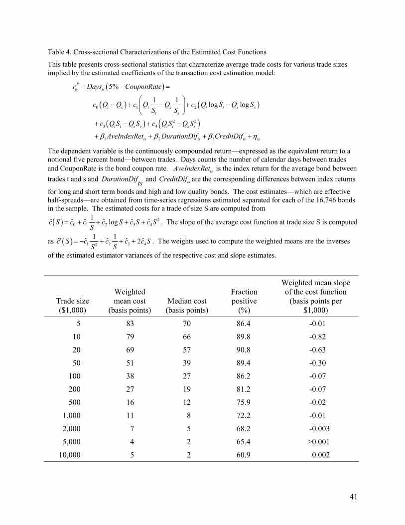
We estimate the transaction cost estimation model (7) separately for all bonds in our

sample. Average customer transaction costs should be positive since customers in dealer

markets generally pay the bid/ask spread when trading. Table 4 shows that a majority of the

estimates are positive for all trade sizes. The fraction that is negative rises with trade size

because large trades are less common than small trades in the sample. The estimates therefore

are less accurate at such sizes. The fraction also rises because large trades apparently are less

costly than small trades.

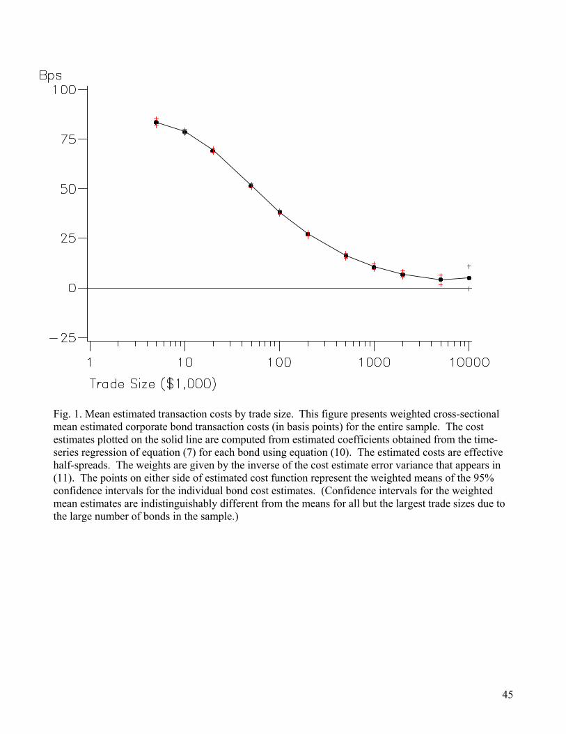
Figure 1 plots cross-sectional mean cost estimates across all bonds in the sample,

weighted by the inverse of their estimation error variances, for a wide range of trade sizes. Also

22 As noted by Harris and Piwowar, the application of this method depends critically on the estimated error variance of the cost estimates. By chance, this variance will be estimated with extreme error when the model is only just barely identified. To avoid this problem, we use the Bayesian shrinkage estimator introduced in the appendix to Harris and Piwowar to estimate regression mean squared errors.

19

plotted is the weighted average of the 95% confidence intervals associated with each bond cost

estimate. As expected, the average confidence interval is widest where the data are sparsest.23

The estimated transaction costs decrease with trade size. The average round-trip

transaction cost for a representative retail order size of 20,000 dollars is 1.38% of price

(69bps × 2), while the average round-trip cost for a representative institutional order size of

200,000 dollars is only 0.54% (27bps × 2). These results may indicate that institutional traders

generally negotiate better prices than do retail traders, or that dealers price their trades to cover

fixed trade costs.

While both explanations may be valid, the shape of the average cost function suggests

that the former explanation is the more important. The OLS fit of

0 11c a aS

= + (13)

to the 11 average cost estimates used to construct the plotted average cost function is extremely

poor (not shown). If the decline in costs with increasing size were simply due to spreading a

fixed cost ( a ) over greater size, this line would closely fit the plotted average cost function.

Although fixed costs probably account for much of the curvature of the average cost function for

small trades, they do not explain the reduction of costs over the entire range.

1

The average cost function could be downward sloped if large traders choose to trade

bonds that are more liquid. The downward sloping average thus may be due to selection rather

than negotiation skills. To rule out this explanation, for each bond, we compute the derivative of

the cost function at various sizes. The last column of Table 4 shows that the average derivative

23 The confidence intervals are for the point estimates of the cost function at given sizes, and not for the cost function as a whole. Since these confidence intervals depend on the same three estimated coefficients, they are highly correlated.

20

is negative, which suggests that the slope of the average is due to the average derivative and not

to sample selection.

The downward sloping cost curve is surprising given the upward sloping costs that

generally characterize all but the largest equity trades.24 We attribute the difference primarily to

the lack of trade transparency in the corporate bond market. Larger traders undoubtedly know

more about values than do smaller traders because they are more likely to be institutional traders

who trade frequently.

Differences in transparency also can explain the differences in average transaction costs

between the two markets. Effective spreads in equity markets for retail sized trades average less

than 40 basis points in contrast to the 138 basis points that we estimate for corporate bonds of

20,000 dollars.25 We cannot reasonably attribute this cost difference to adverse selection

because equities generally are subject to much more credit risk than are corporate bonds. Dealer

inventory considerations probably also cannot explain the differences since the returns to most

corporate bonds are highly correlated with each other and with highly liquid cash and derivative

treasury instruments so that dealers can hedge their positions. Moreover, dealers can also hedge

credit risk using the issuer’s equities. The only credible explanation for the cost difference is the

different market structures, and the most important difference is transparency.

The results we obtain for 2003 TRACE corporate bond sample are very similar to those

obtained in Harris and Piwowar (2005) for the 2000 MRSB municipal bond sample. In both

cases, the estimated cost functions decline significantly with size. However, the estimated bond

trading costs are about 40% lower for the corporate bonds than for the municipal bonds at every

24 Large equity block trades are often arranged by traders (or their brokers) who often know that the trade initiator is not well informed. Costs for such trades are generally lower than they would be if the traders were anonymous to each other.

21

size level. The difference may be due to the different time periods or to the fact that corporate

bonds trade in more active and more transparent markets.26 The difference cannot be due to

differences in credit quality since the average municipal bond is much more secure than the

average corporate bond.

Also, for the comparable transaction sizes, our results are virtually identical to those

obtained in Bessembinder, Maxwell, and Venkataraman (2005). For their sample of insurance

company trades with a mean transaction size of about $3 million, their results indicate a one-way

transaction costs of about 6-7 bps. Our estimates for $2 million trade size is 7 bps and our

estimate for the $5 million 4 bps.

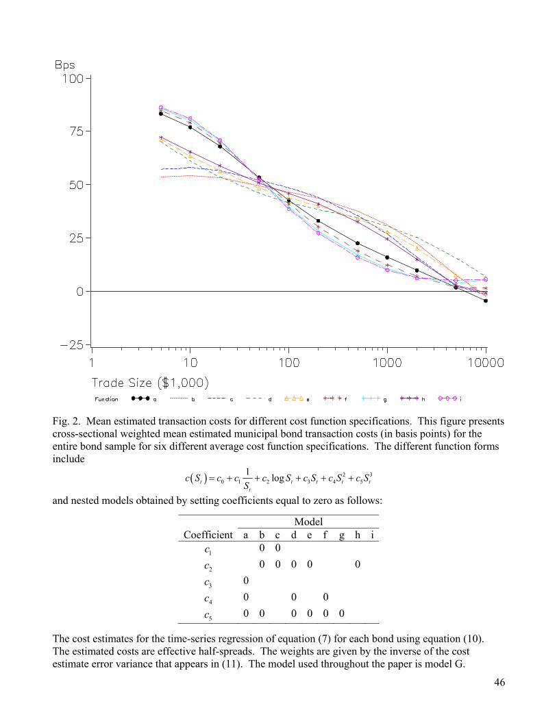
To determine the extent to which the average cost results depend on the functional form

chosen for the cost function, we specified and estimated nine alternative functions. These

alternatives include

( ) 20 1 2 3 4 5

1 logt t tt

c S c c c S c S c S c SS

= + + + + + 3t t

(14)

(14)and various nested models obtained by setting coefficients in to zero. The results reported

in this study are based on the five-parameter model obtained by constraining to zero. Figure 2

plots the nine estimated cost curves. The curves lie very close to each other, which suggests that

the average cost results do not depend much on the chosen functional form. We chose our five-

parameter model because it produced results most similar to the six-parameter model. Harris and

Piwowar use the three-parameter model obtained by setting , , and to zero to conserve

5c

3c 4c 5c

25 Our transaction cost measures estimate effective half spreads. Thus, a cost of 69 basis points represents an effective spread of 138 basis points. 26 During 2000, the MRSB disseminated trade prices only on the next day and only for bonds that traded four times or more on that day.

22

degrees of freedom in their regression model. We chose a larger model because the corporate

bonds are more actively traded than the municipal bonds.

The four panels of Figure 3 present mean estimated cost functions (similar to the mean

cost function presented in Figure 1) computed separately for each class of our four main

classification variables. Panel A plots the mean cost estimates for four transparency classes.

The first class includes bonds for which prices were never transparent during 2003 and the last

class includes bonds for price prices were always TRACE transparent in 2003. The transparent

bonds have lower transaction costs than the opaque bonds, especially for small and large trades.

The other two transparency classes include bonds phased-into TRACE during 2003 (or high-

yield bonds phased-out) and ABS-listed bonds that were never TRACE transparent in 2003. The

bonds that were TRACE transparent for part of 2003 look very much like the fully transparent

bonds, probably because most of these bonds were transparent for ten of the twelve sample

months. The listed bonds have lower transaction costs than the opaque bonds only in the small

trade sizes. This result is likely due to the general perception that ABS is an odd lot market

whose prices are only relevant for small trades.

Results for our four credit quality classes appear in Panel B. Not surprisingly, highly

rated bonds are cheaper to trade than low rated bonds. The difference between the superior and

other investment grade bonds is negligible, but the difference between these two classes and the

speculative grade bonds show that high-yield bonds are almost twice as costly to trade as

investment grade bonds. More striking are the huge transaction costs for defaulted bonds. These

results suggest that adverse selection widens effective spreads in low quality bonds.

Panel C plots mean cost estimates separately for small, medium and large bonds issues.

The smaller bonds have higher transaction costs in all but the smallest trades. The transaction

23

costs for medium bonds are greater than for large bonds for large and small trades, otherwise the

costs of trading these two classes of bonds are quite similar.

Panel D presents results for our three trading activity classes. Interestingly, transaction

costs only appear to be significantly related to trading activity for the most active (an average of

more than 1 trade per day) category. Transaction costs are the highest for this category

throughout the entire retail trade size ranges and some of the institutional trade size range. These

results are surprising since costs are generally lower in active equity markets than in inactive

equity markets.

The results reported in the various panels of Figure 3 are univariate results that do not

control for bond characteristics that may be correlated with trading activity, credit quality, issue

size, transparency, or for the correlations among these characteristics. The next section describes

the regression analyses we use to separately identify the contributions of these (and other)

variables to total transaction costs.

V. Cross-Sectional Determinants of Transaction Costs

This section presents estimation results for regression models that characterize cross-

sectional determinants of transaction costs. The dependent variables are percentage transaction

costs estimated for various representative trade sizes.

Two sources of error contribute to the error terms in these models. The first is due to

error in the transaction costs estimate. The second is due to variation of the data around the

predicted model. We assume that the variance of the former component is proportional to the

estimated error variance of the estimate, and we assume that the variance of the latter component

is constant. We estimate the resulting local variance components model in stages. We first use

WLS to estimate the regression model using weights given by the inverse of the estimated

24

estimate error variances. We then regress the squared residuals on an intercept and the estimated

estimator error variances to estimate the constant and variable variance components.27 Finally,

we reestimate the regression model using the inverses of the predicted values from this

regression as weights. This weighting scheme ensures that we focus the analysis on those bonds

that provide the most information about costs at that size while allowing for typical variation

about the regression model.

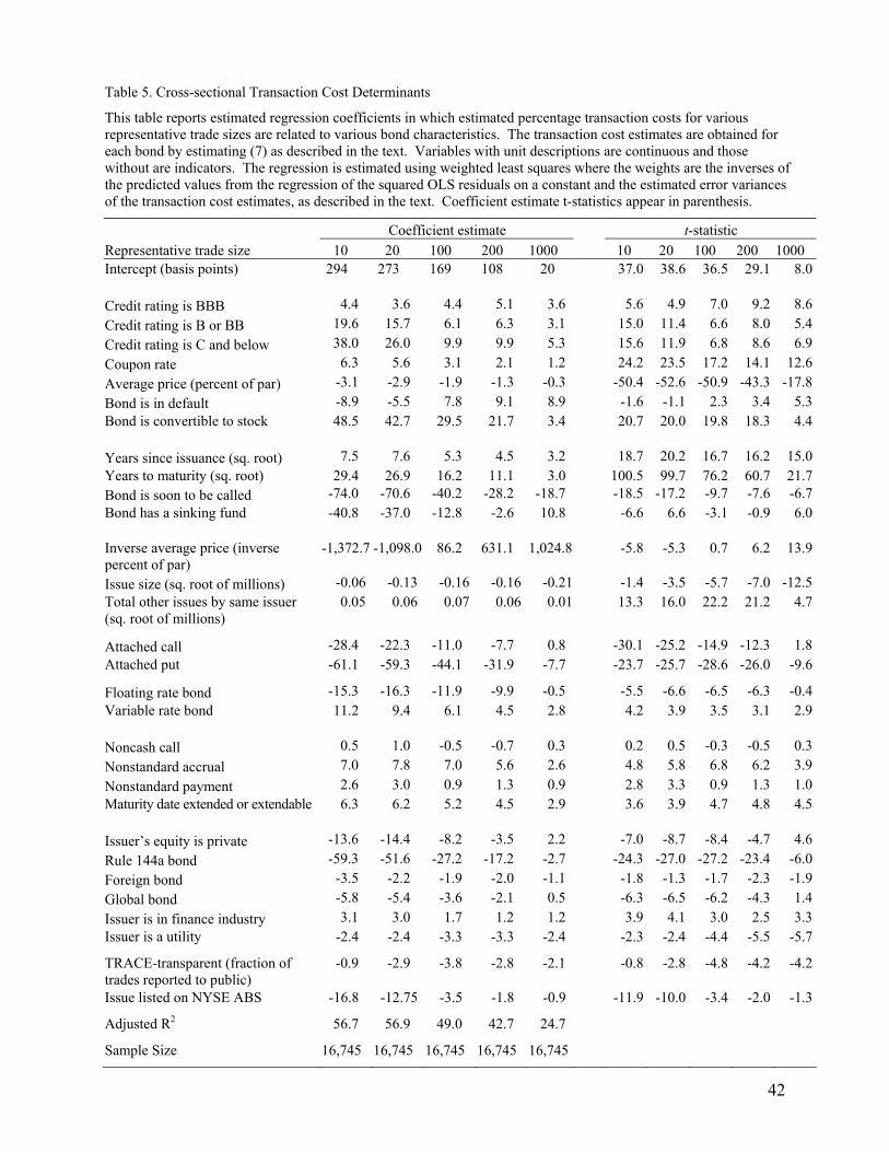
The first set of results presented in Table 5 concern regressors that represent credit

quality. Three dummy variables indicate whether the bond is rated BBB, B or BB, or C and

below. The coefficient estimates indicate that transaction costs increase as credit quality

decreases. For representative trade size of 20 bonds (20,000 dollars), the effective half spread

for BBB bonds is 3.6 basis points more than that of bonds rated A and above. This difference

rises to 16 basis points for other investment quality bonds (B and BB) and to 26 basis points for

speculative bonds (C and below). These differences are all highly statistically significant and are

consistent with the well-known and well-tested adverse selection theory of spreads.

Also included in this set of regressors are other variables that may indirectly indicate

credit quality. Transaction costs are higher for bonds with high coupon rates or low prices. The

former is probably a good proxy for poor credit quality while the later generally reflects market

perception of credit quality. A dummy that indicates whether the issue is in default is highly

significant when the average price variable does not appear in the regression (results not

presented). It is only significantly positive for the estimated transaction costs for large

representative transaction sizes in these regressions. Finally, transaction costs are significantly

higher for convertible bonds than for straight bonds. Convertible bonds are often riskier than

other bonds because they embody credit risk of the underlying stocks.

27 The weights in this estimate are the inverses of the squares of the estimated error variances.

25

The positive and highly significant coefficients on time since issuance indicate that newer

bonds are less expensive to trade than well-seasoned bonds. This result is consistent with well-

known characteristics in the government bond markets in which the costs of trading bonds-on-

the-run trade are lower than the costs of trading seasoned issues.28

The positive and highly significant coefficients on time to maturity indicate that bonds

that mature soon are cheaper to trade than bonds that mature in the distant future. The negative

and highly significant coefficients on dummy variables that represent bond features that decrease

the expected time to maturity—soon to be called and sinking funds—corroborate these results.29

The greater uncertainties associated with valuing long-term bonds as compared to short-term

bonds probably make the long-term bonds more expensive to trade.30

The regression includes inverse price as a regressor to determine whether corporate bond

transaction costs have a fixed cost component. The estimated coefficient is only positive and

significant in the large representative trade size regressions. This regressor, of course, is highly

inversely correlated with the average price regressor. The omission of the latter from the

regression makes the inverse price coefficient positive and highly significant for all trade sizes

(results not reported). It is thus impossible to confidently identify a fixed cost component if

average price is indeed a good proxy for credit quality. Although the results must be interpreted

with caution, the fact that the average price regressor largely knocks out the inverse price

regressor suggests that price probably conveys more information about credit quality than about

fixed costs.

28 See, for example, Sarig and Warga (1989) and Warga (1992). 29 The TRACE data identify a callable bond as soon to be called if the NASD expects that it will be called soon. 30 The bond age and time to maturity variables are transformed by the square root function to shrink large values since we do not expect that a one year difference in these variables has more effect when the values are low than high. We did not use the log transformation for this purpose because it expands low values too much.

26

Large issues have significantly lower transaction costs than do small issues. Although we

expected this result, we note that the effect is not overwhelmingly significant. The weak result

probably is due to the fact that many large bond issues do not trade often.

The total size of other issues outstanding from the same issuer is a significant positive

determinant of transaction cost. This result surprised us because we expected that liquidity in a

given issue would benefit from liquidity in other issues. The result may be due to credit

problems associated with large levered firms.

Bonds with attached calls and with attached puts had significantly lower estimated

transaction costs than those without such features. We found these results surprising since these

features complicate bond valuation. The call results may be explained by the fact that investors

in 2003 undoubtedly expected that many callable bonds would soon be called since yields by

then had dropped significantly since these bonds were issued with high coupons. The bonds thus

would behave more like short term bonds than long term bonds, as so have lower transaction

costs. Indeed, the results reported above for the bonds identified in TRACE as soon to be called

are consistent with this explanation. The bonds most likely to be called are high coupon bonds.

Accordingly, when the product of coupon rate times the call dummy is included in the

regression, the coefficient on the product is significantly negative and the dummy takes a

significantly positive coefficient for all but the large trade sizes (results not reported).31 The put

results may also reflect the fact that the bonds with puts attached will likely be put in the near

future, and so may be valued more like short term bonds than long term bonds.

Floating rate bonds are less expensive to trade than standard bonds. These bonds

generally have less variable prices than standard bonds because the variation in their coupons

27

generally is correlated with variation in bond yields. They therefore should be somewhat easier

to price. Variable rate bonds have coupons that vary according to some schedule. They are

slightly more expensive to trade, probably because of the additional difficulties associated with

pricing them.

Four additional variables that represent bond complexity features—noncash call,

nonstandard accrual, nonstandard payment and extended or extendable maturity date—all are

generally associated with higher bond transaction costs. These features make bonds more

difficult to price and thereby may increase transaction costs. Except for the noncash calls, these

results are all generally statistically significant.

The next regressors characterize the type of bond and the type of issuer. The results

indicate that transaction costs are lower for bonds issued by private issuers (those without

publicly traded equity), Rule 144a issues, foreign bonds, global bonds, and bonds issued by

utilities.32 Bonds issued by financial companies are slightly more expensive to trade. The

private issuer results for small trade sizes are somewhat surprising since the values of these

bonds presumably are harder to determine. However, Alexander, Edwards, and Ferri (2000)

show that the bonds of private issuers trade more frequently than similar bonds from public

issuers and, thus, may be more liquid. The 144a estimate coefficients are very large and highly

significant. Because only large institutions that are Qualified Institutional Buyers (QIBs) can

trade 144a bonds, this result is consistent with the ability of large institutions to negotiate better

prices than can other investors.

31 We did not include this product in the reported regressions because we felt that a proper analysis of this problem would require a full model of the probability that bonds would be called. We attempted to construct such a model, but found that our efforts were severely limited by the data available to us in the TRACE dataset. 32 “Rule 144a” refers to the rule titled ”Rule 144a – Private Resales of Securities to Institutions” promulgated under the Securities Act of 1993, which allows qualified institutional buyers to buy and trade unregistered securities.

28

The final two regressors characterize whether bond prices were transparent in TRACE or

in the NYSE ABS trading system. The estimated coefficients for both variables are significantly

negative, which indicates that transparency is associated with lower transaction costs. The ABS

results are stronger than the TRACE results, probably because ABS prices are immediately

transparent, because ABS quotes are transparent, and because traders may be more used to

looking to ABS than to TRACE for price information. We expect that the TRACE effect would

increase substantially if TRACE data were available more quickly and if it were available for

more bonds. Not surprisingly, the ABS results are also stronger for small trades, which may be

related to the use of ABS for small trades.

Almost all of the quantitative results obtained from these regressions are larger in

absolute value for smaller transaction sizes than for larger sizes. These results suggest that

institutional traders are able to negotiate better prices for bonds of all types than can retail

traders.

Overall, the cross-sectional transaction cost results suggest that corporate bond

transaction costs are negatively related to credit rating and often positively related to instrument

complexity. Younger bonds and bonds with a shorter time-to-expected-maturity are cheaper to

trade than older bonds and bonds with a longer time-to-expected-maturity. These results are

similar to those reported in Harris and Piwowar (2005), although Harris and Piwowar found

stronger results for the complexity measures.

The above analyses show that transparent bonds had lower transaction costs in the 2003

period than did nontransparent bonds, after controlling for many other factors that affect

transaction costs. Although our controls for other factors are quite comprehensive, it is always

possible some omitted variable or some nonlinearity in the population distribution may account

29

for the results.33 In which case, the residuals of the cross-sectional regression would be

correlated so that the significance of our results would be overstated. We address these potential

problems in the next section by analyzing how liquidity varies though time for bonds that were

made TRACE-transparent during our 2003 sample period.

VI. Time Varying Liquidity

This section describes how we estimate and analyze time varying liquidity. The

previously described analyses use separate time series regressions to estimate average transaction

costs for each bond, which we then analyze using cross-sectional regressions. In this section, we

introduce a pooled time series regression model that we use to estimate average transaction costs

for each day for a class of bonds. We estimate the daily average transaction costs for bonds that

were made transparent during 2003, and compare these estimates to those for comparable bonds

that were either TRACE-transparent throughout 2003 or never TRACE-transparent in 2003.

The regression model that we use to estimate daily transaction costs differs only in two

respects from the time series regression model that we used to estimate average transaction costs

for a given bond. First, we specify separate average transaction cost functions, c , for each

day T in the sample. (The functional form, however, is the same for each day.) Second, to

minimize the total number of parameters to be estimated, we use the following three-parameter

average cost function:

( )T tS

34

( ) 0 1 21 logT t T T T t

t

c S c c c SS tκ= + + + . (15)

Second, we model the change in value between bond trades (for a given bond) as

33 In either case, the problem would have to be correlated with our transparency indicator. 34 We also used the five-parameter specification used above and obtained similar, though understandably less powerful results.

30

(16) 1

1log log

T

t s s S J t TJ S

V V f r r f r−

= +

− = + + +∑ ste

where S is the day on which trade s took place and T is the day on which a subsequent trade t

took place, Jr is the common index return (to be estimated) for day J and sf and tf , respectively,

are the fractions of the S and T trading days overlapped by the period spanned by transactions s

and t. This portion of the specification is the same as appears in many paired trade regression

index estimation procedures. With these changes, the regression model is

( )

0 0 1 1 2 2

1

1

5%1 1 log log

Pts ts

T t S s T t S s T t t S s st s

T

s S J t T tsJ S

r Days CouponRate

c Q c Q c Q c Q c Q S c Q SS S

f r r f r η−

= +

− − =

− + − + −

+ + + +∑

(17)

with the variance of tsη given as before by above. As before, we estimate the model in

stages using weighted least squares where the weights are equal to the predicted values of the

regression of the squared residuals on the independent variables appearing in the residual

variation expression.

(9)

Each of the 252 days in the sample adds seven regression coefficients to the model for a

total of 1,764 parameters. To reduce the total estimation time, we estimate the model using a

three-month wide sliding window that we move forward one month at a time. We assemble our

time series of coefficient estimates from the center months of each of the sliding regressions.

For January and December, we respectively use estimates from the first and last regressions.

We compute transaction costs for various representative transaction sizes by evaluating

the estimated transaction cost functions at the representative transaction sizes. Using the

estimated variance-covariance matrix of the estimators, we also compute daily standard errors of

the various daily transaction cost estimates.

31

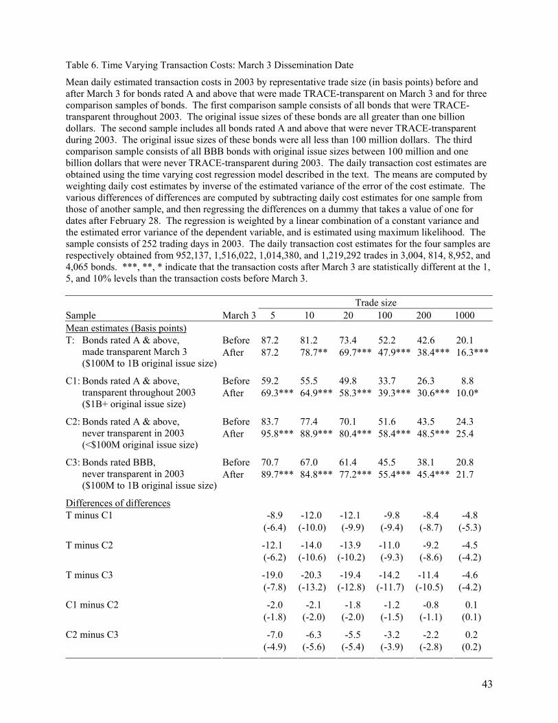
We initially estimate the model for all bonds that the NASD made TRACE-transparent

on March 3, 2003. These include all bonds rated A and above with original issues sizes greater

than 100 million dollars and less than one billion dollars. This sample (T) includes 952,137

trades in 3,004 bonds.

We then estimate the model for three comparison samples. The first comparison sample

(C1) includes all bonds rated A and above that were TRACE-transparent throughout 2003. The

NASD made these bonds transparent on July 1, 2002 because their original issue sizes are greater

than one billion dollars. This sample includes 1,516,022 trades in 814 bonds. The second

sample (C2) includes all bonds rated A and above that were never TRACE-transparent during

2003.35 The original issue sizes of these bonds were all less than 100 million dollars. This

sample includes 1,014,380 trades in 8,952 bonds. The third comparison sample (C3) includes all

BBB bonds with original issue sizes between 100 million and one billion dollars that were never

TRACE-transparent during 2003. This sample includes 1,219,292 trades in 4,065 bonds. The

first two comparison samples consist of bonds with comparable ratings but different issue sizes

whereas the last sample consists of slightly lower grade investment quality bonds of similar size.

We identify the effect of transparency on the bonds that became TRACE-transparent by

comparing daily estimates of their transaction costs with those for the three comparison samples.

The comparison samples thus allow us to control for any time varying changes in liquidity that

might be unrelated to the transparency event. In particular, we compute the daily time series of

differences between average transaction cost estimates for the March 3 bonds and those of each

comparison group. We then separately regress these differences on a dummy variable that

indicates with a value of one for dates (after February 28) on which prices were TRACE-

35 We identify a bond as rated A and above if Moody’s or S&P rated it A or above any time in 2003.

32

transparent. The estimated dummy variable coefficient is a difference of differences. The

standard error of this estimate reflects the time series variation in the differences.

Since the dependent variable is estimated with noise, the residual error of the regression

includes a component that reflects the noise in the dependent variable in addition to a component

that reflects the time series variation in the costs about their mean. We estimate the variance of

the former component from the estimated variance of the cost estimates,36 and assume that the

variance of the latter component is constant. We estimate the resulting model using maximum

likelihood methods.

The results in Table 6 confirm that transparency significantly decreased transaction costs

for the bonds that were made transparent on March 3. Transaction costs decreased in

comparison to each of the three comparison samples. The decrease in transaction costs was

generally greater for smaller trade sizes, most probably because larger traders already had

substantial knowledge of bond values, and hence lower initial transaction costs.

The decrease was greater when measured relative to the bonds that never were made

transparent (C2 and C3) than relative to the bonds that were already transparent (C1). The

relation between the C1 and C2 results is mechanically due to the fact that transaction costs for

the already transparent bonds (C1) fell relative those of the never transparent bonds (C2). This

decrease may be due to traders becoming more aware of the transparent prices, or perhaps to

cross-sectional differences in time varying liquidity that were correlated with original issue size.

However, note that little average difference exists between the two controls samples (C2 and C3)

36 In particular, we sum the estimated variances for the two cost estimates that appear in the difference between cost estimates. The variance of the difference also includes a covariance term that we crudely estimate by correlating the daily cost estimate variances. The results are largely affected by whether we adjust for this covariance or not. The invariance is due to the fact that the estimator error for the April 14 sample is much larger than that of either of the other two samples because the number of trades in the April 14 sample is a small fraction of the numbers in the other samples.

33

for which prices were never transparent despite their cross-sectional differences: C2 consists of

small bond issues rated A and above while C3 consists of intermediate size BBB issues.

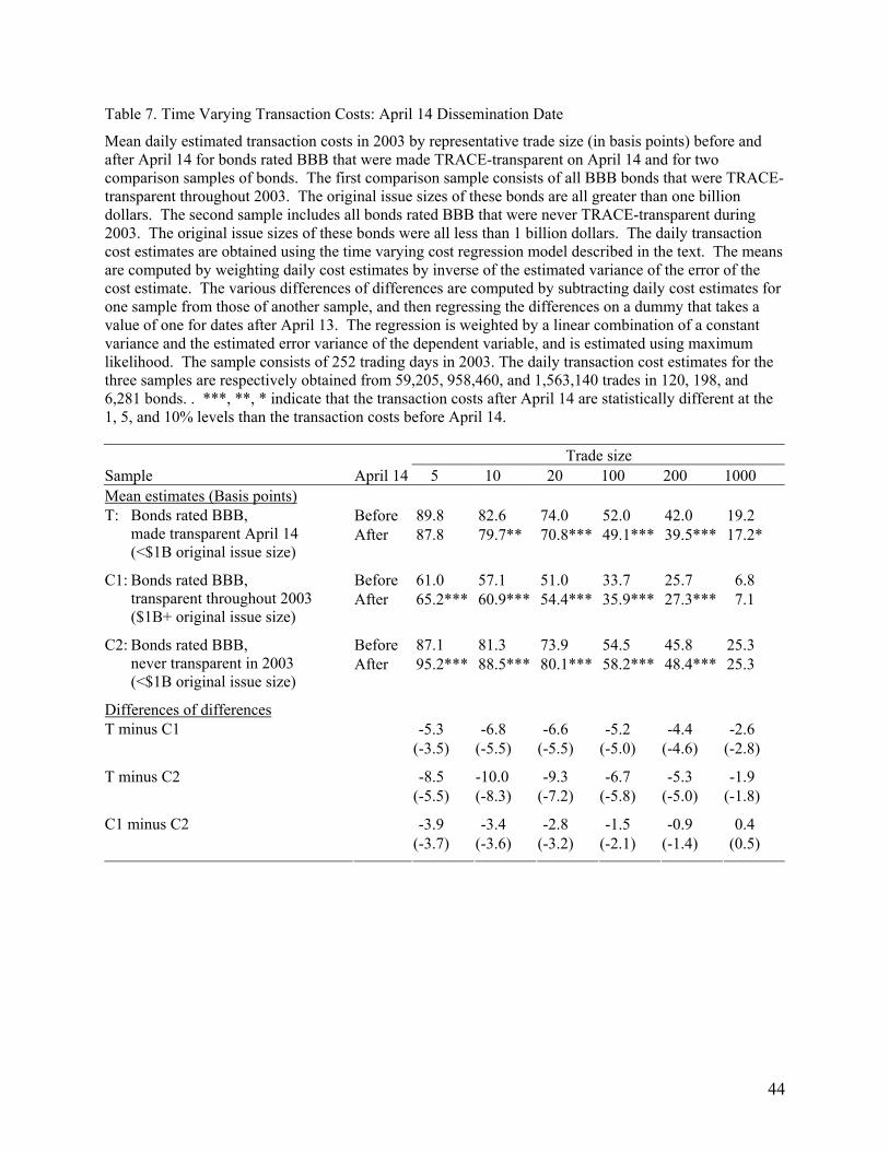
The NASD made 120 intermediate sized BBB rated bonds transparent on April 14.

Using the methods described above, we compared estimated transaction costs in these bonds to

those estimated for comparison samples of all BBB rated bonds that were continuously

transparent and that were never transparent in 2003. The results in Table 7 show that although

the magnitudes of the changes are smaller than those in Table 6, these results are still statistically

and economically significant. The effect of transparency on the transaction costs in these BBB

bonds may have been less than on the intermediate sized A and above bonds because traders may

not have known to look for their prices.

VII. Conclusion

Corporations raise very substantial financing in the bond markets. A better

understanding of the liquidity of these markets thus may help corporations identify ways to lower

their costs of capital. We examine secondary trading costs in the corporate bond market using

improved methods and more comprehensive data than earlier studies. We find that bond price

transparency lowers transaction costs. Accordingly, additional bond transparency may lower

corporate costs of capital.

Our results show that corporate bonds are expensive for retail investors to trade.

Effective spreads in corporate bonds average 1.4% of price for representative retail-sized trades

(20,000 dollars). This is the equivalent of almost three months of total annual return for a bond

with a 6% yield-to-maturity, or 56 cents per share for a 40-dollar stock. If transaction costs are a

deterrent to retail interest, we would expect retail interest to increase with the lower transaction

costs associated with transparency.

34

Unlike in the equity markets, bond transaction costs are much lower for institutional size

transactions. Large traders undoubtedly negotiate better prices because they are better informed

about values than are small investors who rarely trade and who typically lack the analytic

capacity to estimate fundamental bond values. Increased transparency thus would especially

benefit retail investors.

The publication of trade prices for TRACE-transparent bonds occurs as late as 45

minutes after the trade. The effects of transparency on bond transaction costs that we measure

probably thus underestimate the benefits that immediate transparency might produce.

The strongest arguments against transparency involve concerns about how exposure

would make it more difficult for dealers to manage inventory, especially in bonds with poor

credit. The management of inventory problems, however, is easier in the debt markets than in

the equity markets because credit risk is smaller in the former than the latter and because credit

risk can be hedged in the equity markets. Accordingly, given the great liquidity observed in fully

transparent equity markets, and our empirical results, we believe that it would be extremely

unlikely that increased bond market transparency would increase bond transaction costs.

Rather, additional transparency will very likely permit the creation of new market

structures and innovative dealing strategies that will further reduce transaction costs. If so, the

benefits of additional transparency estimated in this paper are far smaller than will likely be

obtained if the corporate bond markets were made more transparent.

35

References Alexander, G., Edwards, A., Ferri, M., 2000, The determinants of trading volume of high-yield corporate bonds, Journal of Financial Markets 3, 177-204. Amihud, Y., Mendelson, H., 1991, Liquidity, maturity, and yields on U.S. Treasury securities, Journal of Finance 46, 1411-1425. Biais, B., Glosten, L., and Spatt C., 2005, Market microstructure: A survey of microfoundations, empirical results, and policy implications, Journal of Financial Markets forthcoming. Bessembinder, H., Maxwell, W., Venkataraman, K., 2005, Optimal market transparency: Evidence from the initiation of trade reporting in corporate bonds, Unpublished working paper. Bloomfield, R. and O’Hara, M., 1999, Market Transparency: Who Wins and Who Loses? Review of Financial Studies 12, 5-35. Blume, M., Keim, D., Patel, S., 1991, Returns and volatility of low-grade bonds, Journal of Finance 46, 49-74. Chakravarty, S., Sarkar, A., 2003, Trading costs in three U.S. bond markets, Journal of Fixed Income 13, 39-48. Chen, L., Lesmond, D., Wei, J., 2002, Bond liquidity estimation and the liquidity effect in yield spreads, Unpublished working paper. Cornell, B., Green, K., 1991, The investment performance of low-grade bond funds, Journal of Finance 46, 29-48. Downing, C., Zhang, F., 2004, Trading activity and price volatility in the municipal bond market, Journal of Finance 59, 899-931. Green, R., Hollifield, B., Schürhoff, N., 2004, Financial intermediation and the costs of trading in an opaque market, Unpublished working paper. Harris, L., Piwowar, M., 2005, Secondary trading costs in the municipal bond market Journal of Finance forthcoming. Hong, G., Warga, A., 2000, An empirical study of bond market transactions, Financial Analysts Journal 56, 32-46. Hotchkiss, E., Ronen, T., 2002, The informational efficiency of the corporate bond market: an intraday analysis, Review of Financial Studies 15, 1325-1354. Hotchkiss, E., Warga A., Jostova, G., 2002, Determinants of corporate bond trading: a comprehensive analysis, Unpublished working paper.

36

Kalimipalli, M., Warga, A., 2002, Bid/ask spread, volatility and volume in the corporate bond market, Journal of Fixed Income 12. Lesmond, D., Ogden J., Trzcinka C., 1999, A new estimate of transaction costs, Review of Financial Studies 12, 1113-1141. Madhavan, A., 2000, Market microstructure: a survey, Journal of Financial Markets 3, 205-208. O'Hara, M., 1997, Market microstructure theory, Basil Blackwell, Cambridge, MA. Sarig, O., Warga, A., 1989, Bond price data and bond market liquidity, Journal of Financial and Quantitative Analysis 24, 367-378. Schultz, P., 2001, Corporate bond trading costs: a peek behind the curtain, Journal of Finance 56, 677-698. Warga, A., 1992, Bond returns, liquidity and missing data, Journal of Financial and Quantitative Analysis 27, 605-616.

37

Table 1. Sample Composition

This table describes the effects of the various filters used to construct the TRACE bond sample analyzed in this study. The data are drawn from the complete 2003 TRACE transaction dataset and from five snapshots of the TRACE master file supplied by the NASD. Securities that did not trade are the issues that appear in the master files but not in the transaction file. TRACE classifies the majority of these bonds as inactive bonds that are not available for trading. We delete any trades that were corrected or duplicate (“corrected trades”), trades with a recorded size that is not an integer, with an execution date prior to the TRACE “First Active Date”, with an execution date after the maturity date or with a recorded size greater than half of the total issue size (“suspect trades”). We classify trades as having suspect prices if they failed to pass filters designed to identify likely data entry errors while allowing for reasonable price changes. Since TRACE requires dealers to report interdealer trades, we delete duplicate records of interdealer trades. Bonds with missing duration information do not have maturity date, coupon rate, or coupon payment frequency information in the TRACE master files. Finally, we remove from the sample those bonds that did not have enough observations to identify the transaction cost regression model that we used to estimate the bond transaction costs.

Bonds Trades Dollar volume

(billions)

Entire TRACE database 68,877 8,668,987 9,413

Less securities that did not trade 46,432 0 0

Less trades with no master matches 14 148 0

Subtotal of securities that traded 22,453 8,668,839 9,412

Less preferred stocks and inactive bonds 59 1,622 2

Subtotal of active bonds 22,394 8,667,217 9,410

Less corrected trades 17,689 718,440 3,073

Subtotal without corrected trades 22,262 7,948,777 6,338

Less suspect trades 3,062 58,605 67

Less suspected pricing data errors 7,215 38,009 22

Subtotal after filtering trades 21,708 7,852,163 5,879

Less duplicate interdealer trades 16,295 1,169,662 718

Less bonds with missing duration information 46 5,036 26

Subtotal after removing duplicate trades 21,662 6,677,465 5,135

Less bonds with unidentified cost regressions 4,916 27,707 56

Final sample 16,746 6,649,758 5,079

38

Table 2. Sample Characteristics

This table summarizes the cross-sectional distributions of volumes and trade sizes for the sample of bonds analyzed in this study. The TRACE sample consists of 6.6 million trades in almost 16,746 corporate bonds. Unless otherwise noted, the statistics summarize means computed for each bond. Retail- and institutional-size trades are respectively identified as those smaller and larger than 100 bonds.

Trading characteristic Mean 1st percentile Median 99th percentile

Mean number of trades per day 1.9 <0.1 0.6 21.9 Interdealer 0.6 0.0 <0.1 7.5 Retail size customer 0.9 0.0 0.2 10.2 Institutional size customer 0.5 0.0 <0.1 5.2 Buy customer volume 0.8 <0.1 0.2 9.3 Sell customer volume 0.5 <0.1 0.2 6.0

Mean dollar volume ($ thousand) 161.9 <0.1 20.6 2,027.4 Interdealer 40.1 0.0 2.7 636.4 Retail size customer 1.8 0.0 0.4 22.8 Institutional size customer 120.0 0.0 14.9 1,455.9 Buy customer volume 62.7 <0.1 8.3 743.0 Sell customer volume 59.1 <0.1 7.5 714.4

Mean annualized turnover (%) 83.0 0.5 51.7 468.5 Interdealer 21.1 0.0 9.8 143.8 Retail size customer 6.0 0.0 1.2 40.7 Institutional size customer 56.0 0.0 26.8 351.3

Frequency of days with a trade (%) 33.2 2.4 23.4 99.6 Interdealer 21.0 0.0 8.3 99.6 Retail size customer 25.3 0.0 13.6 99.6 Institutional size customer 22.1 0.0 8.1 99.6

Trade size in value ($ thousand) 1,154.6 10.1 351.9 12,279.3 Minimum 31.2 0.4 2.0 545.0 Mode 546.2 1.0 11.5 9,806.8 Median 583.5 5.4 29.7 6,806.3 Maximum 12,401.1 25.9 5,091.1 105,242.9 Interdealer 824.1 7.7 192.0 8,440.9 Retail size customer 24.6 4.5 21.5 72.3 Institutional size customer 1,935.4 98.0 1,264.6 15,461.2 Customer buys 1,239.5 8.1 370.0 13,421.6 Customer sells 1,294.0 9.2 425.9 13,005.3 Simple statistics across trades 763.8 1.1 31.2 10,397.0

Mean number of dealers 35.6 2.0 22.0 199.0 Interdealer 17.9 1.0 11.0 110.0 Retail size 12.9 1.0 8.0 74.0 Institutional size 8.7 1.0 6.0 37.0

39

Table 3. Cross-sectional Bond Characteristics This table characterizes the cross-sectional distributions of various bond features in the TRACE data. A bond is classified as transparent if it is transparent at any point in 2003. Credit quality is based on the average credit quality during 2003. A bond is classified as defaulted if it was in default at any point in 2003. The bonds are classified into age categories based on their average age in 2003. S&P assigns the industrial classification of a bond with respect to the nature of the bond and not that of the issuer. Equity status refers to whether the bonds issuer has publicly traded equity in the US. Subsidiaries have the same equity status as their parent. Bonds in sample Trades in sample Total value traded Feature Number Percent Thousands Percent $ Billions Percent Bond transparency

TRACE-disseminated 3,719 22.2 3,279 49.3 2,712 53.4 ABS-listed 444 2.7 306 4.6 171 3.4 Both ABS and TRACE 185 1.1 157 2.4 112 2.2 Not transparent 12,768 76.2 3,222 48.4 2,308 45.4

Credit quality Superior (AA and up) 1,559 9.3 496 7.5 412 8.1 Other investment grade (BBB-A) 10,520 62.8 4,164 62.6 2,906 57.2 Speculative (below BBB) 3,891 23.2 1,752 26.4 1,575 31.0 Not Rated 428 2.6 81 1.2 97 1.9 Defaulted 490 2.9 157 2.4 89 1.8

Issue size Small (< $100 million) 6,728 40.2 854 12.8 65 1.3 Medium ($100 - $500 million) 7,801 46.6 2,257 33.9 1,633 32.2 Large (> $500 million) 2,268 13.5 3,539 53.2 3,380 66.6

Age 0-3 months 3,334 19.9 696 10.5 804 15.8 3-6 months 1,115 6.7 478 7.2 620 12.2 6 months- 1 year 1,350 8.1 532 8.0 449 8.9 1 year – one-half life 6,222 37.2 3,393 51.0 2,404 47.3 one-half life – maturity 4,725 28.2 1,551 23.3 801 15.8

Industry Finance 8,230 49.1 3,028 45.5 1,915 37.7 Utilities 6,254 37.3 3,001 45.1 2,594 51.1 Other 2,298 13.7 621 9.3 569 11.2

Equity status Publicly Traded in US 15,307 91.4 6,308 94.9 4,721 92.9 Private or Foreign 1,439 8.6 342 5.1 358 7.1

Bond complexity features Callable 5,710 34.1 1,693 25.7 1,173 23.0 Non-cash Call 567 3.4 118 1.8 89 1.8 Putable 736 4.4 248 3.7 442 8.7 Sinking Fund 342 2.0 28 0.4 38 0.8 Convertible 896 5.4 4,549 6.8 635 12.5 Extendible 16 0.1 2 <0.1 6 0.1 Paid in Kind 12 0.1 1 <0.1 1 <0.1 Floating Rate Coupon 704 4.2 61 0.9 310 6.1 Variable Rate Coupon 340 2.0 101 1.5 123 2.4 Combination of floating/fixed 30 0.2 5 <0.1 13 0.3 Nonstandard payment frequency 3,586 21.4 648 9.7 532 10.5 Nonstandard accrual frequency 852 5.1 260 3.9 444 8.7

Type of issue Global 2,493 14.9 2,735 41.1 2,303 45.3 Euro 3 <0.1 <0.1 <0.1 <0.1 <0.1 Foreign 833 5.0 198 3.0 285 5.6 Rule 144a issue 1,521 9.1 271 4.1 672 13.2

Asset status Soon to be called 571 3.4 27 0.4 15 0.3 Reopened 232 1.4 603 9.1 453 8.9 Defeased 3 <0.1 0.3 <0.1 <0.1 <0.1

40

Table 4. Cross-sectional Characterizations of the Estimated Cost Functions

This table presents cross-sectional statistics that characterize average trade costs for various trade sizes implied by the estimated coefficients of the transaction cost estimation model:

( )

( ) ( )

( ) ( )

0 1 2

2 23 4

1 2 3

5%

1 1 log log

Pts ts

t s t s t t s st s

t t s s t t s s

ts ts ts ts

r Days CouponRate

c Q Q c Q Q c Q S Q SS S

c Q S Q S c Q S Q S

AveIndexRet DurationDif CreditDifβ β β

− − =

− + − + −

+ − + −

+ + + η+ The dependent variable is the continuously compounded return—expressed as the equivalent return to a notional five percent bond—between trades. Days counts the number of calendar days between trades and CouponRate is the bond coupon rate. is the index return for the average bond between trades t and s and

tsAveIndexRetDurationDifts and are the corresponding differences between index returns

for long and short term bonds and high and low quality bonds. The cost estimates—which are effective half-spreads—are obtained from time-series regressions estimated separated for each of the 16,746 bonds in the sample. The estimated costs for a trade of size S are computed from

tsditDifCre

( ) 2ˆ0 1 41ˆ ˆ ˆc S c c c SS

= + +

( )

2 3ˆ ˆlogc S c S+ + . The slope of the average cost function at trade size S is computed

as 1 2 31 1ˆ ˆ 2c c cS S

+ + + 42ˆ ˆ ˆc S c S′ = − . The weights used to compute the weighted means are the inverses

of the estimated estimator variances of the respective cost and slope estimates.

Trade size ($1,000)

Weighted mean cost

(basis points) Median cost (basis points)

Fraction positive

(%)

Weighted mean slope of the cost function

(basis points per $1,000)

5 83 70 86.4 -0.01

10 79 66 89.8 -0.82

20 69 57 90.8 -0.63

50 51 39 89.4 -0.30

100 38 27 86.2 -0.07

200 27 19 81.2 -0.07

500 16 12 75.9 -0.02

1,000 11 8 72.2 -0.01

2,000 7 5 68.2 -0.003

5,000 4 2 65.4 >0.001

10,000 5 2 60.9 0.002

41

Table 5. Cross-sectional Transaction Cost Determinants

This table reports estimated regression coefficients in which estimated percentage transaction costs for various representative trade sizes are related to various bond characteristics. The transaction cost estimates are obtained for each bond by estimating (7) as described in the text. Variables with unit descriptions are continuous and those without are indicators. The regression is estimated using weighted least squares where the weights are the inverses of the predicted values from the regression of the squared OLS residuals on a constant and the estimated error variances of the transaction cost estimates, as described in the text. Coefficient estimate t-statistics appear in parenthesis.

Coefficient estimate t-statistic Representative trade size 10 20 100 200 1000 10 20 100 200 1000 Intercept (basis points) 294 273 169 108 20 37.0 38.6 36.5 29.1 8.0

Credit rating is BBB 4.4 3.6 4.4 5.1 3.6 5.6 4.9 7.0 9.2 8.6Credit rating is B or BB 19.6 15.7 6.1 6.3 3.1 15.0 11.4 6.6 8.0 5.4Credit rating is C and below 38.0 26.0 9.9 9.9 5.3 15.6 11.9 6.8 8.6 6.9Coupon rate 6.3 5.6 3.1 2.1 1.2 24.2 23.5 17.2 14.1 12.6Average price (percent of par) -3.1 -2.9 -1.9 -1.3 -0.3 -50.4 -52.6 -50.9 -43.3 -17.8Bond is in default -8.9 -5.5 7.8 9.1 8.9 -1.6 -1.1 2.3 3.4 5.3Bond is convertible to stock 48.5 42.7 29.5 21.7 3.4 20.7 20.0 19.8 18.3 4.4

Years since issuance (sq. root) 7.5 7.6 5.3 4.5 3.2 18.7 20.2 16.7 16.2 15.0Years to maturity (sq. root) 29.4 26.9 16.2 11.1 3.0 100.5 99.7 76.2 60.7 21.7Bond is soon to be called -74.0 -70.6 -40.2 -28.2 -18.7 -18.5 -17.2 -9.7 -7.6 -6.7Bond has a sinking fund -40.8 -37.0 -12.8 -2.6 10.8 -6.6 6.6 -3.1 -0.9 6.0

Inverse average price (inverse percent of par)

-1,372.7 -1,098.0 86.2 631.1 1,024.8 -5.8 -5.3 0.7 6.2 13.9

Issue size (sq. root of millions) -0.06 -0.13 -0.16 -0.16 -0.21 -1.4 -3.5 -5.7 -7.0 -12.5Total other issues by same issuer (sq. root of millions)

0.05 0.06 0.07 0.06 0.01 13.3 16.0 22.2 21.2 4.7

Attached call -28.4 -22.3 -11.0 -7.7 0.8 -30.1 -25.2 -14.9 -12.3 1.8Attached put -61.1 -59.3 -44.1 -31.9 -7.7 -23.7 -25.7 -28.6 -26.0 -9.6

Floating rate bond -15.3 -16.3 -11.9 -9.9 -0.5 -5.5 -6.6 -6.5 -6.3 -0.4Variable rate bond 11.2 9.4 6.1 4.5 2.8 4.2 3.9 3.5 3.1 2.9

Noncash call 0.5 1.0 -0.5 -0.7 0.3 0.2 0.5 -0.3 -0.5 0.3Nonstandard accrual 7.0 7.8 7.0 5.6 2.6 4.8 5.8 6.8 6.2 3.9Nonstandard payment 2.6 3.0 0.9 1.3 0.9 2.8 3.3 0.9 1.3 1.0Maturity date extended or extendable 6.3 6.2 5.2 4.5 2.9 3.6 3.9 4.7 4.8 4.5

Issuer’s equity is private -13.6 -14.4 -8.2 -3.5 2.2 -7.0 -8.7 -8.4 -4.7 4.6Rule 144a bond -59.3 -51.6 -27.2 -17.2 -2.7 -24.3 -27.0 -27.2 -23.4 -6.0Foreign bond -3.5 -2.2 -1.9 -2.0 -1.1 -1.8 -1.3 -1.7 -2.3 -1.9Global bond -5.8 -5.4 -3.6 -2.1 0.5 -6.3 -6.5 -6.2 -4.3 1.4Issuer is in finance industry 3.1 3.0 1.7 1.2 1.2 3.9 4.1 3.0 2.5 3.3Issuer is a utility -2.4 -2.4 -3.3 -3.3 -2.4 -2.3 -2.4 -4.4 -5.5 -5.7

TRACE-transparent (fraction of trades reported to public)

-0.9 -2.9 -3.8 -2.8 -2.1 -0.8 -2.8 -4.8 -4.2 -4.2

Issue listed on NYSE ABS -16.8 -12.75 -3.5 -1.8 -0.9 -11.9 -10.0 -3.4 -2.0 -1.3

Adjusted R2 56.7 56.9 49.0 42.7 24.7

Sample Size 16,745 16,745 16,745 16,745 16,745

42

Table 6. Time Varying Transaction Costs: March 3 Dissemination Date

Mean daily estimated transaction costs in 2003 by representative trade size (in basis points) before and after March 3 for bonds rated A and above that were made TRACE-transparent on March 3 and for three comparison samples of bonds. The first comparison sample consists of all bonds that were TRACE-transparent throughout 2003. The original issue sizes of these bonds are all greater than one billion dollars. The second sample includes all bonds rated A and above that were never TRACE-transparent during 2003. The original issue sizes of these bonds were all less than 100 million dollars. The third comparison sample consists of all BBB bonds with original issue sizes between 100 million and one billion dollars that were never TRACE-transparent during 2003. The daily transaction cost estimates are obtained using the time varying cost regression model described in the text. The means are computed by weighting daily cost estimates by inverse of the estimated variance of the error of the cost estimate. The various differences of differences are computed by subtracting daily cost estimates for one sample from those of another sample, and then regressing the differences on a dummy that takes a value of one for dates after February 28. The regression is weighted by a linear combination of a constant variance and the estimated error variance of the dependent variable, and is estimated using maximum likelihood. The sample consists of 252 trading days in 2003. The daily transaction cost estimates for the four samples are respectively obtained from 952,137, 1,516,022, 1,014,380, and 1,219,292 trades in 3,004, 814, 8,952, and 4,065 bonds. ***, **, * indicate that the transaction costs after March 3 are statistically different at the 1, 5, and 10% levels than the transaction costs before March 3. Trade size Sample March 3 5 10 20 100 200 1000 Mean estimates (Basis points)

Before 87.2 81.2 73.4 52.2 42.6 20.1 T: Bonds rated A & above, made transparent March 3 ($100M to 1B original issue size)

After 87.2 78.7** 69.7*** 47.9*** 38.4*** 16.3***

Before 59.2 55.5 49.8 33.7 26.3 8.8 C1: Bonds rated A & above, transparent throughout 2003 ($1B+ original issue size)

After 69.3*** 64.9*** 58.3*** 39.3*** 30.6*** 10.0*

Before 83.7 77.4 70.1 51.6 43.5 24.3 C2: Bonds rated A & above, never transparent in 2003 (<$100M original issue size)

After 95.8*** 88.9*** 80.4*** 58.4*** 48.5*** 25.4

Before 70.7 67.0 61.4 45.5 38.1 20.8 C3: Bonds rated BBB, never transparent in 2003 ($100M to 1B original issue size)

After 89.7*** 84.8*** 77.2*** 55.4*** 45.4*** 21.7

Differences of differences -8.9 -12.0 -12.1 -9.8 -8.4 -4.8 T minus C1 (-6.4) (-10.0) (-9.9) (-9.4) (-8.7) (-5.3)

T minus C2 -12.1 -14.0 -13.9 -11.0 -9.2 -4.5

(-6.2) (-10.6) (-10.2) (-9.3) (-8.6) (-4.2)

T minus C3 -19.0 -20.3 -19.4 -14.2 -11.4 -4.6

(-7.8) (-13.2) (-12.8) (-11.7) (-10.5) (-4.2)

-2.0 -2.1 -1.8 -1.2 -0.8 0.1 C1 minus C2 (-1.8) (-2.0) (-2.0) (-1.5) (-1.1) (0.1)

-7.0 -6.3 -5.5 -3.2 -2.2 0.2 C2 minus C3 (-4.9) (-5.6) (-5.4) (-3.9) (-2.8) (0.2)

43

Table 7. Time Varying Transaction Costs: April 14 Dissemination Date

Mean daily estimated transaction costs in 2003 by representative trade size (in basis points) before and after April 14 for bonds rated BBB that were made TRACE-transparent on April 14 and for two comparison samples of bonds. The first comparison sample consists of all BBB bonds that were TRACE-transparent throughout 2003. The original issue sizes of these bonds are all greater than one billion dollars. The second sample includes all bonds rated BBB that were never TRACE-transparent during 2003. The original issue sizes of these bonds were all less than 1 billion dollars. The daily transaction cost estimates are obtained using the time varying cost regression model described in the text. The means are computed by weighting daily cost estimates by inverse of the estimated variance of the error of the cost estimate. The various differences of differences are computed by subtracting daily cost estimates for one sample from those of another sample, and then regressing the differences on a dummy that takes a value of one for dates after April 13. The regression is weighted by a linear combination of a constant variance and the estimated error variance of the dependent variable, and is estimated using maximum likelihood. The sample consists of 252 trading days in 2003. The daily transaction cost estimates for the three samples are respectively obtained from 59,205, 958,460, and 1,563,140 trades in 120, 198, and 6,281 bonds. . ***, **, * indicate that the transaction costs after April 14 are statistically different at the 1, 5, and 10% levels than the transaction costs before April 14. Trade size Sample April 14 5 10 20 100 200 1000 Mean estimates (Basis points)

Before 89.8 82.6 74.0 52.0 42.0 19.2 T: Bonds rated BBB, made transparent April 14 (<$1B original issue size)

After 87.8 79.7** 70.8*** 49.1*** 39.5*** 17.2*

Before 61.0 57.1 51.0 33.7 25.7 6.8 C1: Bonds rated BBB, transparent throughout 2003 ($1B+ original issue size)

After 65.2*** 60.9*** 54.4*** 35.9*** 27.3*** 7.1

Before 87.1 81.3 73.9 54.5 45.8 25.3 C2: Bonds rated BBB, never transparent in 2003 (<$1B original issue size)

After 95.2*** 88.5*** 80.1*** 58.2*** 48.4*** 25.3

Differences of differences -5.3 -6.8 -6.6 -5.2 -4.4 -2.6 T minus C1 (-3.5) (-5.5) (-5.5) (-5.0) (-4.6) (-2.8)

T minus C2 -8.5 -10.0 -9.3 -6.7 -5.3 -1.9

(-5.5) (-8.3) (-7.2) (-5.8) (-5.0) (-1.8)

-3.9 -3.4 -2.8 -1.5 -0.9 0.4 C1 minus C2 (-3.7) (-3.6) (-3.2) (-2.1) (-1.4) (0.5)

44

Fig. 1. Mean estimated transaction costs by trade size. This figure presents weighted cross-sectional mean estimated corporate bond transaction costs (in basis points) for the entire sample. The cost estimates plotted on the solid line are computed from estimated coefficients obtained from the time-series regression of equation (7) for each bond using equation (10). The estimated costs are effective half-spreads. The weights are given by the inverse of the cost estimate error variance that appears in (11). The points on either side of estimated cost function represent the weighted means of the 95% confidence intervals for the individual bond cost estimates. (Confidence intervals for the weighted mean estimates are indistinguishably different from the means for all but the largest trade sizes due to the large number of bonds in the sample.)

45

Fig. 2. Mean estimated transaction costs for different cost function specifications. This figure presents cross-sectional weighted mean estimated municipal bond transaction costs (in basis points) for the entire bond sample for six different average cost function specifications. The different function forms include

( ) 2 30 1 2 3 4 5

1 logt t tt

c S c c c S c S c S c SS

= + + + + +t t

and nested models obtained by setting coefficients equal to zero as follows:

Model Coefficient a b c d e f g h i

1c 0 0

2c 0 0 0 0 0

3c 0

4c 0 0 0

5c 0 0 0 0 0 0 The cost estimates for the time-series regression of equation (7) for each bond using equation (10). The estimated costs are effective half-spreads. The weights are given by the inverse of the cost estimate error variance that appears in (11). The model used throughout the paper is model G.

46

Panel A: Transparency classes Panel B: Credit rating classes

Panel C: Issue size classes Panel D: Trading activity classes Fig. 3. Mean estimated transaction costs for various bond classifications. This figure presents weighted cross-sectional mean estimated corporate bond transaction costs (in basis points) computed separately for various bond classifications. The cost estimates are computed from estimated coefficients obtained from the time-series regression of equation (7) for each bond using equation (10). The estimated costs are effective half-spreads. The weights are given by the inverse of the cost estimate error variance that appears in (11). Bonds in the low, medium, high, and very high trade activity classes respectively have 1 or fewer transactions per week; between 1 transaction per week and 1 transaction per day, and more than 1transaction per day. Bonds in the superior, other investment, and speculative credit quality classes respectively include bonds rated AA and above, BBB to A, and below BBB. The small, medium and large issue size classes respectively include bonds smaller than one hundred million dollars, between 100 and 500 million dollars, and above 500 million dollars.

47