Corporate Governance and Value Creation: Evidence...

0

Corporate Governance and Value Creation:

Evidence from Private Equity1

by

Viral V. Acharya, Oliver Gottschalg, Moritz Hahn and Conor Kehoe

First draft: 7 April 2008 This draft: 2 June 2011

Contact information:

Viral V. Acharya

NYU-Stern, NBER, CEPR and ECGI Stern School of Business, 44 West 4th St, New York, NY 10012

Tel: +1 212 998 0354 e-mail: [email protected]

Oliver F. Gottschalg

HEC School of Management, Paris 78351 Jouy-en-Josas, France

Tel: +33 (0) 670017664 e-mail: [email protected]

Moritz Hahn

Schellingstr. 88, 80798 Munich, Germany Tel: +49 (0) 176 1275 8319

e-mail: [email protected]

Conor Kehoe McKinsey & Company, Inc.

1 Jermyn Street, London – SW1Y 4UH, UK Tel: +44 (0) 20 7961 5988

e-mail: [email protected]

1 A part of this study was undertaken while Viral Acharya was at London Business School and partly while visiting Stanford-GSB. We are especially grateful to the PE firms who assembled and gave us access to sensitive deal data. Viral Acharya was supported during this study by the London Business School Governance Center and Private Equity Institute, the Leverhulme Foundation, INQUIRE Europe, and London Business School's Research and Materials Development (RAMD) grant. Oliver Gottschalg was supported by the HEC Foundation. McKinsey & Company also devoted significant human resources to carrying out the fieldwork and analysis, not for any client but on its own account. We are grateful to excellent assistance and management of data collection and interviews by Amith Karan, Ricardo Martinelli, Prashanth Reddy and David Wood of McKinsey & Co. Ramin Baghai-Wadji, Ann Iveson, Hanh Le, Chao Wang and Yili Zhang also provided valuable research assistance. The study has benefited from comments of two anonymous referees, Laura Starks (editor), Yael Hochberg (discussant), Steve Kaplan (discussant), Tim Kelly (discussant) and seminar participants at European Central Bank and Centre for Financial Studies Conference (2008) in Frankfurt, Inaugural Symposium (2008) at London Business School’s Coller Institute of Private Equity, University of Chicago and University of Illinois at Chicago joint conference, London Business School, McKinsey & Co., Western Finance Association Meetings (2008), and participating PE firms. All errors remain our own.

1

Corporate Governance and Value Creation: Evidence from Private Equity

Abstract

We examine deal-level data from 395 private equity transactions in Western Europe

initiated by large private equity houses during the period 1991 to 2007. We un-lever the deal-

level equity return and adjust for un-levered return to quoted peers to extract a measure of

abnormal performance of the deal. The abnormal performance is significantly positive on

average, and stays positive in periods with low sector returns. In the cross-section of deals,

higher abnormal performance is related to greater growth in sales and greater improvement in

EBITDA to sales ratio (margin) during the private phase, relative to those of quoted peers.

Finally, we show that general partners with an operational background (ex-consultants or ex-

industry-managers) generate significantly higher outperformance in organic deals that focus

exclusively on internal value creation programs; in contrast, general partners with a

background in finance (ex-bankers or ex-accountants) generate higher outperformance in

deals with significant M&A events. We interpret these findings as evidence, on average, of

positive, but heterogeneous skills at deal partner level in private equity transactions.

JEL: G31, G32, G34, G23, G24.

Keywords: leveraged buyouts (LBO), management buyouts (MBO), active ownership,

activism

2

1. Introduction

In a seminal piece on private equity, Jensen (1989) argued that leveraged buyouts

(LBOs) create value through high leverage and powerful incentives. He proposed that public

corporations are often characterized by entrenched management that is prone to cash-flow

diversion and averse to taking on efficient levels of risk. Consistent with Jensen’s view,

Kaplan (1989), Smith (1990), Lichtenberg and Siegel (1990), and others provide evidence

that LBOs create value by significantly improving the operating performance of acquired

companies and by distributing cash in the form of high debt payments.

By contrast, the recent literature has focused on the returns that private equity (PE)

funds – which usually initiate the LBO and own, or more precisely manage, at least a majority

of the resulting private entity – generate for their end investors such as pension funds. In

particular, Kaplan and Schoar (2005) studied internal rates of return (IRRs) net of

management fees for 746 funds during 1985-2001 and found that the median fund generated

only 80% of S&P500 return and the mean was only slightly higher, at around 90%. 2

Our paper is an attempt to bridge these two strands of literature concerning PE, the

first of which analyses the operating performance of acquired companies, and the second that

analyzes fund IRRs. In addition, we investigate how human capital factors are associated with

However, the evidence suggests that returns are better for the largest and most mature houses

– those that have been around for at least 5 years. Kaplan and Schoar note that, for funds in

this sub-set of PE houses, the median performance is 150% of S&P500 return and the mean is

even higher at 170%. Furthermore, this performance is persistent, a characteristic that is

generally associated with potential existence of “skill” in a fund manager. It is interesting to

note that such persistence has rarely been found in mutual funds, and when found has

generally been in the worst performers (Carhart, 1997).

2 This evidence have been replicated by studies in Europe (Phalippou and Gottschalg, 2009, Phalippou, 2007), though they raise the issue of certain survivorship biases in data employed which might imply no median outperformance relative to the market even for large and mature PE houses. This by itself does not necessarily refute Jensen’s original claim; it could simply be that PE funds keep the value they create through fees. The puzzle that the evidence on median return of PE funds raises is thus more about why their investors (the limited partners) choose to invest in this asset class as a whole, an issue investigated by Lerner and Schoar (2004) and Lerner, Schoar and Wong (2007).

3

value creation in PE deals. We focus on the following questions: (1) Are the returns to large,

mature PE houses simply due to financial leverage over and above comparable quoted sector

peers, or do these returns represent the value created in enterprises they engage with (so-

called “portfolio companies”), over and above the value created by the quoted sector peers?

(2) What is the effect of ownership by large, mature PE houses on the operating performance

of portfolio companies relative to that of quoted peers, and how does this operating

performance relate to the financial value created (if any) by these houses? (3) Are there any

distinguishing characteristics of PE houses or partners involved in a deal that are best

associated with value creation?

To answer the first question, we develop a methodology to break down the deal-level

equity return, measured by the IRR, into two components: the un-levered return, and

amplification of this un-levered return by deal leverage. Next, we subtract from the un-

levered deal return, the un-levered return that the quoted peers of the deal generated over the

life of the deal. The difference between these two un-levered returns is what we call

“abnormal performance”: a measure of enterprise-level outperformance of the deal relative to

its quoted peers, after removing the effects of financial leverage. We hypothesize, and later

show, that the abnormal performance of a deal captures the return associated with changes in

operating performance of the portfolio company, and human capital factors such as deal

partner skills.

We apply this methodology to 395 deals closed during the period 1991 to 2007 in

Western Europe by 37 large, mature PE houses (each with funds larger than ~$300mln)3

3 We believe this time period is particularly well-suited for studying value creation through operational engineering. Kaplan and Stromberg (2008) note that operational engineering became a key private equity input to portfolio companies primarily in the last decade.

; the

mean, gross IRR for this sample is 56.1%. We find that, on average, about 34% (19.8 out of

56.1%) of average deal IRR comes from abnormal performance, another 50% (27.9 out of

56.1%) is due to higher financial leverage, and the remaining portion (16 out of 56.1%) is due

to exposure to the quoted sector itself. Although abnormal performance has substantial

variation across deals, it is on average positive and statistically significant, even during

4

periods of low sector returns; this is consistent with the view that large, mature PE houses

generate higher (enterprise-level) returns compared to benchmarks. In the cross-section of

deals, abnormal performance has a positive, albeit imperfect, correlation to IRR and to the

“public-market equivalent” (PME) measures employed by Kaplan and Schoar (2005), and a

negative correlation to sector returns.

Regarding the second question, we find a positive impact of ownership by large,

mature PE houses on the operating performance of portfolio companies, relative to that of the

sector. In particular, during PE ownership the deal margin (EBITDA/Sales) increases by

around 0.4% p.a. above the sector median; and the deal multiple (EBITDA/Enterprise Value)

increases by around 1 (or 16%) above the sector median. We interpret the operational

improvements as causal PE impact, since we find no evidence for a violation of the strict

exogeneity assumption of the PE acquisition decision. That is, we assume – and later confirm

– that there is nothing inherent in the companies targeted by the PE firms in our sample, that

would have caused their operating performance to improve without being acquired by Private

Equity.4

We then provide evidence that higher abnormal performance is associated with a

stronger operating improvement in all operating measures relative to quoted peers: we find

In addition, we examine the impact of major M&A events during the private phase

on operational performance during the same period, since M&A events can generate – due to

their direct impact on the operational measures – a considerable distortion of underlying

operational performance. However, we still find margin and multiple improvements above

sector when we analyze deals with and without M&A events separately.

4 For example, in theory, what we label as “operational improvements” could in fact be the reversion of the acquired deals’ performance to the mean. However, we find evidence against the mean-reversion argument: although the sample size of deals with more than 2 years of pre-acquisition data is small, they show no difference to their respective sector companies in performance trends pre-acquisition: both targeted and sector companies show nearly the same increase in nominal sales and constant profitability. Yet, PE might still be able to identify companies that will be subject to a positive future shock. This is something we can not rule out. However, a systematic relationship between PE-ownership and anticipated future performance shocks can induce abnormal performance in PE deals. To financially exploit individual shocks on a company, a PE house must have a systematic informational advantage in forecasting the future in comparison to the seller and other bidding PE houses. This systematic informational advantage appears questionable in a competitive buyout market, such as that for the large sized firms in Western Europe.

5

that sales growth, EBITDA margin and multiple improvement are important explanatory

factors for abnormal performance.

Overall, this evidence is consistent with top, mature PE houses creating financial

value through operational improvements. Such improvements require skill, and the return to

such skill may explain the persistent returns generated by these funds for their investors

(Kaplan and Schoar, 2005).

This brings us to our final question where we study whether deal partner

characteristics affect the performance of PE deals. We use deal partner background as a

human capital, or skill, factor that may be relevant to deal success; the econometric advantage

of using this factor is that it is fixed, or time-invariant, and hence exogenous (except for the

matching of deal partners to specific deals).

We find evidence that there are combinations of value creation strategies and partner

backgrounds that correlate with deal-level abnormal performance. Deal partners with a strong

operational background (e.g., ex-consultants or ex-industry-managers) generate significantly

higher outperformance in “organic” deals. In other words, partners who worked as managers

in the industry or as management consultants before joining a PE house seem to have

gathered skills to improve a company internally, for example, through cost-cutting, or

expansion to new customers and new geographies. In contrast, partners with a background in

finance (e.g., ex-bankers or ex-accountants) more successfully follow an M&A-driven, or

“inorganic”, strategy.

One could argue that we only studied deals from the funds we sampled, which might

have been cherry-picked by the PE fund. We show that this is not the case. While we have a

bias in our sample for large PE funds, this is by design given that we wished to understand

drivers of their persistent out-performance. However, within the funds we sampled for our

deals, we find no statistically significant bias between the performance of deals sampled and

those not sampled.5

5 Moreover, in contrast to the extant literature that mainly focuses on public-to-private deals, our data set also covers deals where only part of a company is acquired (e.g., carve-out deals), and private-to-

6

In Section 2, we review the related literature. In Section 3, we provide a description

of the data we collected and some summary statistics. In Section 4, we describe the

methodology for calculating abnormal performance. In Section 5, we discuss operating

performance. In Section 6, we link abnormal performance and operating performance. Section

7 discusses the role of deal partner background. Section 8 concludes.

2. Related literature

Following the seminal work of Jensen (1989) on LBOs, the early empirical

contributions verified the impact of PE ownership on firms (Kaplan, 1989; Smith, 1990;

Lichtenberg and Siegel, 1990). 6

private deals, where a non-listed business is acquired. Using carve-out and private-to-private deals is important, because they comprise 74% of PE deals in Western Europe over the last decade, and they are different in size (enterprise value) and profitability (EBITDA margin) from public-to-private deals (according to a simple, non-statistical, analysis of data provided by Private Equity Insight).

However, the most recent wave of PE transactions (2001-

mid-2007) has prompted researchers to re-examine whether buyouts are still creating value in

this new era. Guo, Hotchkiss and Song (2009) answer this question with a sample of 94 US

public-to-private transactions between 1990 and 2006. They find that gains in operating

performance are not statistically different from those observed for benchmark firms. Also

Leslie and Oyer (2008) find weak or generally no evidence of greater profitability or

operating efficiency of 144 LBOs in the US between 1996 and 2004, relative to public

companies. However, Lerner, Sorensen and Stromberg (2008) provide evidence with a

sample of 495 buyouts that, in contrast to the oft-cited claim that PE has short-term

incentives, buyout deals in fact lead to significant increases in long-term innovation. They

find that patents applied for by firms in PE transactions are more frequently cited (a proxy for

economic importance), show no significant shifts in the fundamental nature of the research,

and are more concentrated in the most important and prominent areas of companies'

innovative portfolios.

6 Note that Kaplan (1989), Smith (1990), and Lichtenberg and Siegel (1990) also investigate whether LBOs improved operating performance at the expense of workers. They find that the wealth gains from LBOs were not a result of significant employee layoffs or wage reductions (see Palepu (1990) for a detailed survey of these papers and Kaplan and Stromberg (2008) also for a comprehensive survey).

7

This literature has focused mainly on the data from the US whereas our data are based

on PE deals in the UK and Europe. Several studies have examined LBOs in the UK, which

also experienced a tremendous increase in buyout activity prior to the crisis of 2007-09.

Nikoskelainen and Wright (2005) study 321 exited buyouts in the UK in the period 1995 to

2004. On average, these deals generated a 22% return to enterprise value and 71% return to

equity, after adjusting for market return. In a related paper, Renneboog, Simons, and Wright

(2007) examine both the magnitude and sources of the expected shareholder gains in 177 UK

public-to-private, transactions from 1997 to 2003. They find that pre-transaction shareholders

receive a premium of 40%. They also find that the main sources of post-transaction gains in

shareholder wealth are undervaluation of the pre-transaction target firm, increased interest tax

shields, and realignment of incentives. Harris, Siegel, and Wright (2005) study the

productivity of UK manufacturing plants subject to management buyouts (MBO). Such plants

experienced substantial increases in productivity, the post-MBO magnitudes of which are

substantially higher than those reported in the US, for example, by Lichtenberg and Siegel

(1990).

In limited evidence regarding human capital or skill factor in PE investments, Kaplan

et al. (2008) analyze the relationship between 316 portfolio company managers (CEOs) and

the success of buyouts. They find that execution skills appear to be more strongly related to

success than interpersonal skills. To our knowledge, with the exception of this study, there

has been no systematic analysis of the link between financial returns of LBOs and human

capital factors. As Cumming et al. (2007) state “… there is a need to understand the human

capital expertise that successful PE firms require. There appears to be a need to broaden the

traditional financial skills base of private equity executives to include more product and

operations expertise.”

Our evidence regarding the relevance of human capital factors and, in particular,

regarding task-specific deal partner skills (operational or financial) fills this important gap in

the literature for PE investments. We posit that task-specific skills attributable to deal partner

background are one significant part of the persistent abnormal financial return generated by

8

large, mature PE houses for their investors (Kaplan and Schoar, 2007). 7

In contrast, for venture capital (VC) investments, it seems to in be an established fact

that VC funds have an impact on the development of new companies, and that expertise of the

fund matters for performance. Hellmann and Puri (2002), for example, show that VC funds

add professional structure and rigor to the start-ups in which they invest, namely that: start-

ups backed by VC funds replace their CEOs more frequently; introduce stock option plans;

and hire a VP of sales and marketing. Dimov and Shepard (2005) find a positive relationship

between successful, VC-backed IPOs and the education of senior managers in the VC fund in

science or humanities. Moreover, experience of management consulting reduces the share of

bankruptcies for individual funds. Bottazzi et al. (2008) go one step further and provide

evidence that experience in consulting or industry on the part of VC fund managers predicts

investor activism – for instance the frequency of interaction between the VC fund and start-up

– and seems to correlate with performance.

PE partners seem to

add value to portfolio companies by applying skills they have accumulated over time.

Most recently, Zarutskie (2010) argues that, not only is prior business experience

relevant to the performance of VC fund investments, but also longevity in the VC industry.

According to the author, task-specific human capital factors seem to be most important and

depend on the type of investment: fund managers with science backgrounds only excel in

high-tech investments; while those with finance backgrounds excel in later-stage investments.

Again, it is important to note that such returns to task-specific skills gathered over time are

not found for mutual fund managers, which seldom hold majority stakes and therefore engage

less actively in the management of the portfolio company (Chevalier and Ellison, 1999).

3. Data and sample selection

Our sample combines two data sets. First, we use proprietary deal-level data collected

together with McKinsey (McKinsey sample), a consulting company which serves large PE

7 We note that our paper is silent about the conflicts of interest between private equity houses and their investors. Axelson et al. (2009), Ljunqvist et al. (2007) and Metrick and Yasuda (2007) provide good coverage of theoretical as well as empirical issues on this front.

9

houses. The McKinsey sample is relatively small (n=110), but gives detailed deal-level

information, e.g., operational performance measures prior to PE ownership. The second data

set was provided by a major investor in PE funds (LP sample), that has tracked the detailed

performance of PE investments over the last two decades. The LP sample is larger (n=285),

but covers less information.

The McKinsey sample represents relatively large deals, with enterprise values greater

than roughly €50 million and all acquired by fourteen large, mature PE houses from 1995 to

2005. To collect the data, we approached 40 large, well established, European multi-fund

houses, active in either “mid-cap” or “large-cap” markets, of which 14 (35%) agreed to

provide data – subject to confidentiality (all data herein are aggregated and not attributable to

any single deal or PE house). Together, these firms provided data for 110 deals, with each

group of deals pertaining to a specific fund checked by us to ensure the performance, or

average IRR, of each group was representative of the fund from which they were drawn.

Where groups of deals failed this test, we removed or replaced a small number of deals to

meet this condition. For individual deals, we rigorously checked data, looking for

discrepancies (e.g., in currencies, sales, cash flows, etc.) and followed up with PE houses

when necessary.

The LP data set is drawn from hand-collected track records of private equity firms

reported in fund raising documents (PPM) of the PE funds. In the PPMs, we observe the list

of the investments made by each PE firm. Out of the pool of PPMs collected by the LP, we

selected 34 from large, well established, European multi-fund houses, active in either “mid-

cap” or “large-cap” markets. The LP data set has the additional advantage of being audited

rather than self-reported. Importantly, buyout firms generally disclose in PPMs all the

investments they made including the ones that do not perform well. As a consequence, this

sample contains numerous poorly performing investments. From these 34 PPMs, we collected

all 285 realized transactions for which both cash flows and operating performance were

available. Again each group of deals pertaining to a specific fund was checked by us to ensure

10

the performance, or average IRR, of each group was representative of the fund from which

they were drawn.

The final combined dataset comprises 395 deals from 48 funds covering nearly two

decades. For each deal, we have the exact structure of cash flows, from and to the parent fund,

and detailed data on financial and operating measures. We do not have all enterprise level

cash flows, which would include for example also taxes or interest and principal paid on

debt.8

To compare our sample to a set of publicly listed peers we collected data, supplied by

Datastream, for circa 7,000 publicly listed corporations (PLCs) in Europe, from which we

constructed sector indices based on ICB (Industry Classification Benchmark)_sector codes;

these codes group publicly listed peers into 10 industries and 39 sectors. We collected data on

TRS (Total Returns to Shareholders); enterprise value; net debt; equity; sales; and

EBITDA(E) – the latter to remove the effects of exceptional items, which are not included in

EBITDA figures provided by the firms in our sample.

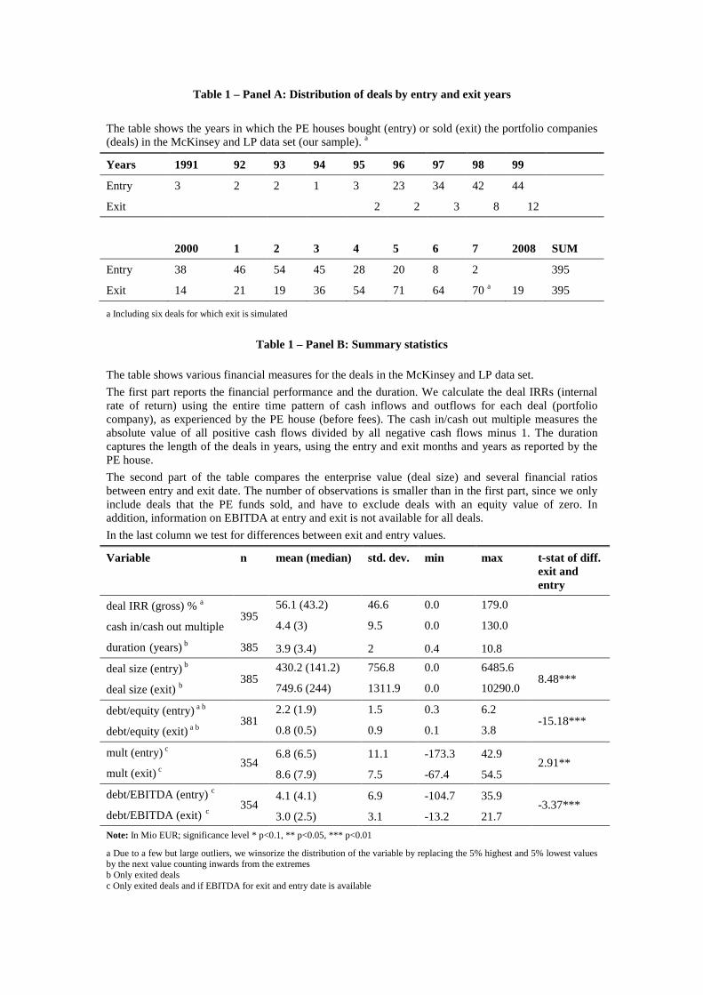
Table 1, Panel A shows that, within our sample period (1991-2008), our deals are

well spread-out over time, although there is some concentration in 1998-2003 in terms of

deal entry or acquisition. Table 1, Panel B provides additional summary statistics for the

deals. Deals in our sample have a high mean, gross IRR (56.1%) and cash multiple (4.4),

with large values on the right tail, even winsorizing our sample (we replace the lowest 5% of

values with the 5th percentile value, and the highest 5% with the 95th percentile value).

However, a high value for average IRR is to be expected from a sample of deals from large,

mature PE houses (Kaplan and Schoar, 2005). We also report an average duration of 3.9

years.

8 We also do not have all cash flows for 6 un-exited deals in the McKinsey data set because there is no exit cash flow from sale, nor can it be deemed to be zero as in the case of bankruptcies. Therefore, the end enterprise-value cash flow was simulated using the EV / EBITDA multiple at the start of the deal and applying that number to 2006 or 2007 year-end EBITDA. Our results are robust to alternative assumptions, including one assumption that they produced no terminal cash flow whatsoever. However, we have verified that such a pessimistic scenario is unlikely to be appropriate for these deals.

11

In the second half of Table 1, Panel B we compare financial ratios at the entry and

exit date. The median entry EV/EBITDA multiple is 6.5, whereas the corresponding exit

multiple is 7.9, which indicates that on average, assuming stable or rising EBITDA(E), our

deals improved their market valuations (consistent with the findings of Kaplan, 1989). The

median debt-to-equity (D/E) ratio at entry is 1.9, which is in line with the usual LBO capital

structure, believed to be 70% debt and 30% equity (Axelson et al., 2008). However, the

median D/E ratio at exit is much smaller (0.5). In percentage terms, the median debt-to-

EBITDA ratio, which falls from 4.1 at entry to 2.5 at exit, does not fall as much as the median

D/E ratio. Consistent with Groh and Gottschalg (2011), it appears that the debt to equity ratio

falls for PE deals during their life only partly due to improvements in coverage ratio

(Debt/EBITDA), and mainly due to improvements in equity value over deal life.

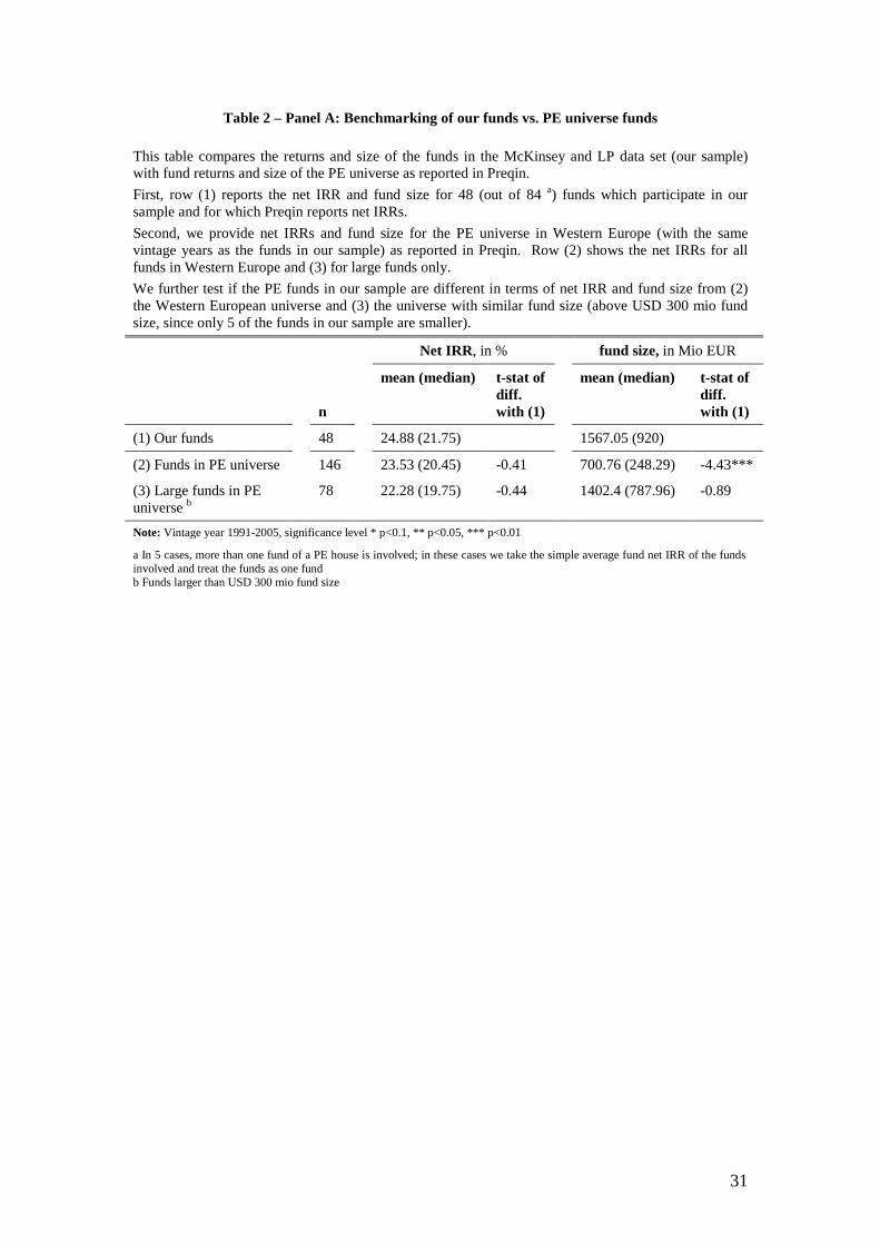
Next, we come to the important sample-selection issues. Table 2, Panel A-C provides

several relevant comparisons between our sample and the PE universe. Overall, we conclude

that our sample covers mainly large funds, but seems to be representative in terms of

performance, and includes all different vendor types, that is, not just public-to-private deals

but also the frequent private-to-private deals.

First, Table 2, Panel A shows that the sampled funds are a good representation of

funds in Western Europe, also when we take into account the fact that we are focusing on

funds whose sizes are above $300 million. All 146 funds in Western Europe with the vintage

year in 1991-2005 as our sample have a simple average net IRR of 23.5% (based on 146

funds for which Preqin reports IRRs), which is not different to the net IRR of our funds (t-

statistic = -0.41 for the difference). Also large funds in the PE universe (again, for which

Preqin reports IRRs) have similar returns than our funds (t= -0.44 for the difference).

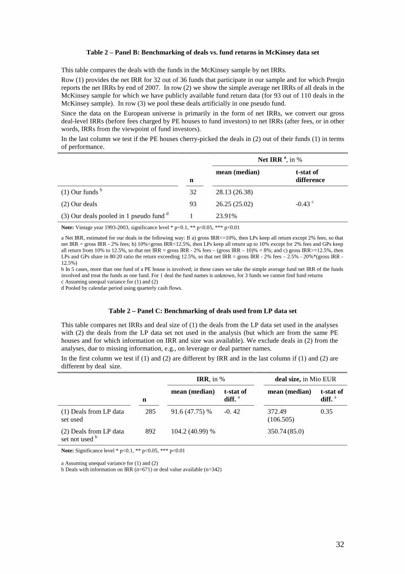
In Table 2, Panels B and C provide evidence that we have not cherry-picked the deals

out of the funds we have sampled. Table 2, Panel B compares the average performance of the

deals in the McKinsey sample, per fund (in terms of net IRR), to the performance of the same

32 funds from which our deals were drawn; average fund IRRs are based on Preqin figures.

We show that the funds in the McKinsey sample do not appear to have cherry-picked the

12

deals that they reported: the difference between the average publicly reported net fund IRR of

28.1% and the average net IRR of our deals, per fund, of 26.3% is not statistically significant

(t=0.43). In terms of deal performance, therefore, we have an unbiased representation of

deals within the funds we sampled. For the comparison, because publicly available data on

fund performance is based on net IRRs, we had to convert our gross deal-level IRRs, prior to

fees and carry paid to the PE funds by investors, to net IRRs – or IRRs from the viewpoint of

fund investors 9. We deduct from the gross IRR a 2% annual fee and 20% carry for IRR

above the typical benchmark, market return, of 8%10

Table 2, Panel C shows a similar result for the LP data set. That is, there is no

statistical difference between the LP deals we selected (n=285) and those made by the same

PE houses we didn’t select (n=892), both in terms of performance (t=-0.42 for the difference)

and size (t=0.35 for the difference); the deals we selected were chosen because they provided

us with the requisite financial data, and because the names of the deal partners were available,

allowing us to determine their backgrounds.

.

Finally, as previously mentioned, our sample includes all types of deals, which is

important to get a full perspective on the effects of PE ownership. The extant literature

mainly focuses on public-to-private transactions, which is only a part of the total buyout

activity in Western Europe. By contrast, the majority of deals are carve-outs where only part

of a company is acquired, or private-to-private deals, where PE firms acquire a non-listed

business. For example, in Western Europe carve-out and private-to-private deals comprise

more than two-thirds of all PE transactions (between 1995 and 2005) – and they are smaller in

size and different in profitability (EBITDA margin) from public-to-private deals in the 9 To perform this conversion, we also construct an artificial fund of our sample deals and calculate its IRR. The pseudo-fund starts in 1995 and lasts for 13 years, until 2007. Investments or cash inflows take place in years 1-9 (with small investments in years 10 and 11 as well). The bulk of the investments occur in years 3-9. Cash payouts start in year 5; in the last 3 years, the fund only has cash payouts. Using this pattern of cash inflows and outflows, we calculate the gross IRR of the pseudo-fund. 10 More specifically, if a) gross IRR<=10%, then LPs keep all return except 2% fees, so that net IRR = gross IRR - 2% fees; b) 10%<gross IRR<12.5%, then LPs keep all return up to 10% except for 2% fees and GPs keep all return from 10% to 12.5%, so that net IRR = gross IRR - 2% fees – (Gross IRR – 10%) = 8%; and c) gross IRR>=12.5%, then LPs and GPs share in 80:20 ratio the return exceeding 12.5%, so that net IRR = gross IRR - 2% fees - 2.5% - 20%*(gross IRR - 12.5%). The pooled net IRR for our deals is 23.9%, which is close to the average net deal IRR of 26.2%.

13

Western European universe (according to a simple, non-statistical, analysis of data provided

by Private Equity Insight).

4. A measure of abnormal financial performance

4.1 Methodology

One of the key questions we want to answer in this study is how much of the excess

returns generated by PE firms, relative to quoted peers, comes from pure financial leverage,

and how much comes from genuine operational improvements. To disentangle the effect of

leverage from that of operational improvements, we first calculate the IRR of the deal і – its

levered return (RL,i) – using the entire time series of gross cash flows for the deal (i.e. before

fees), both from and to the fund as recorded by the PE house. Then we un-lever this IRR. and

benchmark this un-levered return (RU,i) to returns for the quoted peers of the deal, unlevered

in the same way (RSU,i). The resulting difference in un-levered returns is what we call the

“abnormal performance” of the deal (also referred to as “alpha” in earlier drafts of the paper).

To arrive at the unlevered return RU,I we use:

)/1()/)(1(,,

,i

iiDiLiU ED

EDtRRR

+

−+= (1)

The un-levered IRR, RU,i , corresponds to the return generated at the enterprise level.

Since the PE houses in our sample did not report RD,i , the average cost of debt D, we use the

base rate and interest margin spread reported in Dealogic for each deal.11

11 Dealogic provides information on the base rate and the interest margin spread for only 67 deals (out of 110) in our sample. For 19 deals we can find only the base rate (Libor vs. Euribor) and for the remaining 24 deals we find no information. If the margin spread is unknown, we use the median spread of all PE deals in Western Europe in the same year. If the base rate is unknown, we use LIBOR for the UK deals and Euribor for all other deals.

The leverage ratio

D/Ei is the average of the entry and exit debt-to-equity ratio of the deal; that is, since the

starting D/E is higher than exit D/E for most deals we employ the average of the two to reflect

We made sure that the assumption on the spread does not have a large impact on our results. First, the spread does not vary much in the cross-section. In our sample period and for all deals covered in Dealogic, the standard deviation of the weighted (by risk tranches) average spread is 1.1%, with an average (median) spread of 2.6 (2.3) % (n=984). Second, the sensitivity of the abnormal performance of a deal to different interest rate assumptions is less than 1. It varies according the un-levering formula by (D/E)/ (1+D/E) * Δi. For example, with a D/E ratio of 2, a Δi of 1 bp increase of the interest rate only changes the abnormal performance by 2/3 bp.

14

the pattern of declining leverage for most deals. Finally, for tax rate t, we use the average

corporate tax rate during the holding period for the country in which the portfolio company’s

headquarters is located.

We also apply (1) to calculate un-levered sector IRRs, RSU,I, from the benchmark

levered sector return, RS,i. In this case, a sector is defined as containing all quoted European

“peer” companies sharing the deal’s 3-digit ICB (Industry Classification Benchmark) code in

Datastream. To do so, we first calculate RS,i – the median annualized total return to

shareholders (TRS) for the sector over the life of each deal, which we un-lever using (1) and

the median D/E for the sector over a three-year average from the deal’s entry date onwards.

We further assume the same tax rate and cost of debt for the sector as for the deal. From (1), it

follows that higher values of RD,i result in greater un-levered return for the same levered

return. Since RD,i for the sector companies is potentially lower than for the deals (due to lower

leverage and hence lower risk), we overestimate the un-levered sector returns and are

therefore conservative in attributing positive abnormal performance to PE deals.

After obtaining the un-levered returns for both the deal (RU,i ) and sector (RSU,i ),

which are stripped of the effects of financial leverage, the next key step is to measure the

amount of excess PE return that is brought about by genuine operational improvements. For

this purpose, we define the abnormal performance of the deal, iα , as:

, ,i U i SU iR Rα = − (2)

In essence, applying (1) and (2) allows us to make the following decomposition or

performance attribution of each deal IRR:

(i) Deal-level abnormal performance: iα

(ii) Unlevered sector performance: ,SU iR

(ii) Total leverage effect: iUiL RR ,, −

The leverage effect )( ,, iUiL RR − measures the total effect of leverage on deal return.

However, we are more interested in measuring the effect of the additional leverage that

15

companies take on after their acquisition by PE. To arrive at the incremental effect of

increased leverage, we first re-write (1) in terms of RL,i as follows:

)/)(1()/1( ,,, iiDiiUiL EDtREDRR −−+=

Then, we substiture for RU,i based on (2):

)/)(1()/1()/1()/)(1()/1)((

,,

,,,

iiDiiSUii

iiDiiSUiiL

EDtREDREDEDtREDRR−−+++=

−−++=

α

α

And finally, substitute for D/Ei in terms of incremental leverage:

)//(// ,, iSiiSi EDEDEDED −+=

To arrive at the following decomposition of deal IRR:

)]/()//))(1([()]/)(1()/1([

,,,

,,,,

,

iiiSiiDiSU

iSiDiSiSU

iiL

EDEDEDtRREDtREDR

R

α

α

+−−−

+−−+

+=

This equation provides an alternative decomposition of each deal IRR:

(i) Deal-level abnormal performance: iα measures the excess asset return generated at the

enterprise level of the portfolio company for PE investors, purged of the effect of leverage.

(ii) Levered sector return: , , , ,(1 / ) (1 )( / )SU i S i D i S iR D E R t D E+ − − measures the effect of

contemporaneous sector returns, including the effect of leverage inherent in the sector.

(iii) Return from incremental leverage: , , ,( (1 ))( / / ) ( / )SU i D i i S i i iR R t D E D E D Eα− − − +

captures the amplification effect that a) the incremental deal leverage beyond the sector

leverage, (D/Ei – D/ES,i), has on sector returns and b) the total leverage has on abnormal

performance.

Finally the decomposition also allows us to quantify the tax benefits of the

incremental leverage in private equity transactions, which is , ,( / / )D i i S it R D E D E− .

The purpose of performing such a decomposition, or return attribution, is three-fold.

First, it is to see if the sample deals from mature PE houses generated a significantly positive

abnormal performance on average or not. Second – if we believe that the abnormal

performance is attributable to operating strategies and changes attempted by the PE firms –

16

what is the cross-sectional distribution of this abnormal performance? And third – and

perhaps most importantly – is there evidence at the individual deal level that abnormal

performance is related to measures of operational improvement, and to the characteristics of

PE houses or their deal partners?

Before we proceed to discussing our results, it is useful to note some of the

limitations of our methodology. First, it treats leverage as having a purely financial effect

rather than having some incentive effect. Second, our methodology is subject to the usual

problems associated with IRRs, namely that they are a way of describing cash flows rather

than actual, realized returns, and that they translate into returns only under extreme

assumptions of constant and common discount rates and reinvestment rates. To address the

second issue, another approach we adopted was to calculate a public market equivalent (PME)

for each deal. As a benchmark, we used the sector return to discount all cash flows and then

calculated the ratio of discounted cash flows to the largest cash inflow for the deal (in the

spirit of Kaplan and Schoar, 2005). We discuss the relationship between our measure of

abnormal performance, IRR and PME in the next section. Finally, since we do not have the

exact cash payouts on debt, we are unable to employ the methodology of Kaplan (1989),

which is to simulate the enterprise-level (not equity) cash flows that would be obtained by

investing these cash inflows in the quoted sector and examining the cash outflows thus

generated. We chose to use IRR, given its simplicity and also because it is easily broken

down into abnormal performance and related components.

4.2. Average abnormal performance and its characteristics

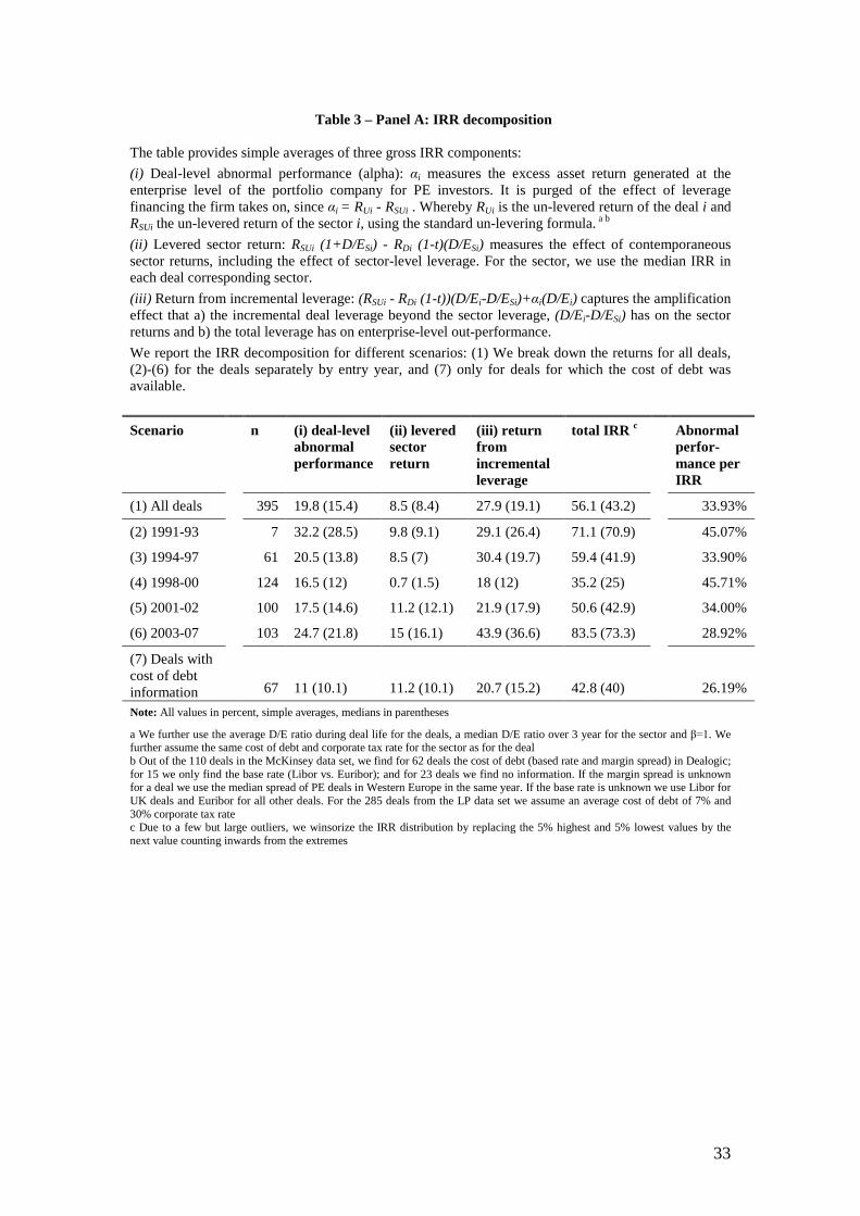
Table 3, Panel A summarizes the results from employing the decomposition method

of Section 4.1. It presents results for (1) the overall sample of 395 deals; (2) – (6) for

different time periods; and (7) the set of 67 deals out of the McKinsey sample for which we

were able to find the exact cost of debt for the deals in Dealogic. The key findings are as

follows:

Out of the average IRR of 56.1% for all 395 deals, sector risk and leverage

amplification on this accounts for a total of 8.5%. In other words, less than one fifth of the

17

total return is attributable to either the sector-picking ability of PE houses or simply to pure

luck. The incremental leverage effect of 27.9% is due to high deal leverage, relative to

comparatively low sector leverage. The average abnormal performance of 19.8% is

statistically significant (at a 1% level), confirming that large, mature PE houses do in fact

generate higher (enterprise-level) returns compared to benchmarks, and that not all of these

are attributable to sector exposure and financial leverage. The medians tell a similar story.

Abnormal performance stays statistically significant (at a 1% level), when we cluster

the deals by entry date. Even in years with very low sector returns as in row (4), PE was able

to generate abnormal performance. The high return from incremental leverage in row (6)

might correspond to availability of cheap debt financing, a phenomenon believed to be at

work especially for PE deals struck during 2003 to mid-2007 and likely responsible for the

somewhat high valuation multiples paid by PE houses during 2003-07 (Acharya, Franks and

Servaes, 2007; and Kaplan and Stromberg, 2008)

Abnormal performance is also positive and statistically significant for the 67 deals for

which we have data on the cost of debt (via Dealogic) although the abnormal performance of

11.0% for these deals is lower than that for all deals (19.8%). This is partly explained by

trends in the availability of data; that is, cost of debt is typically only available for later deals,

and, on the whole, abnormal performance declines over our sample period.

Overall, the evidence points to outperformance of PE deals in our sample in a manner

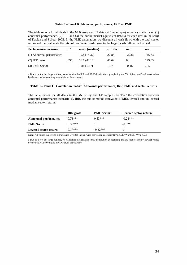
that is robust to alternative measures. In Table 3, Panel B we provide IRR and PME,

alternative measures of deal performance. Consistent with our earlier results – which showed

that PE firms in our sample generate positive abnormal performance – our deals also display

high IRRs and PME returns relative to both the sector and overall market e.g. the average

sector PME is 188%. In Table 3, Panel C, as one might expect abnormal performance is

positively correlated with both IRR and sector PME, albeit imperfectly, with correlation

coefficients of 0.73 and 0.53 respectively. Interestingly, though, abnormal performance is

negatively correlated with sector returns.

18

5. Operating performance

5.1. Operating measures

The next step in our analysis is to see if, at the enterprise level, abnormal financial

performance is related to abnormal operating performance. Abnormal operating performance

can be displayed in two ways: as a larger EBITDA growth rate of the portfolio company

during PE ownership compared to pre-acquisition; or as a larger EBITDA growth rate after

PE ownership compared to the sector. To disentangle the PE impact on EBITDA during PE

ownership, we focus on the effects on (1) sales and (2) profitability (margin=EBITDA/Sales).

We capture the impact on the company after the PE ownership period by analyzing (3) the

EBITDA multiple (Enterprise Value/EBITDA) at time of exit from the deal. Here, we have to

rely on the assumption that market expectations are rational at exit, since we do not have

operational figures after the PE phase for many of the deals (trade sales, for example).

The three measures we analyze in detail are: 12

(1) Sales, equal to operating revenues earned in the course of ordinary operating activities.

(2) Margin (EBITDA/Sales). EBITDA (Earnings before Interest, Taxes, Depreciation and

Amortization) is equal to Operating revenues - COGS (cost of goods sold) - SG&A (selling,

general and administrative expenses) - Other (e.g., R&D) = Operating income. Note that

EBITDA is commonly used as it shows a company's fundamental operational earnings

potential. However, EBITDA is not a defined measure according to Generally Accepted

Accounting Principles (GAAP) or IFRS/IAS. In the present paper, we define EBITDA

excluding “Non-operating income.” 13

12 Since we work with operational numbers in €, we convert all figures into € at the exchange rate applicable in that year.

Often this measure is more precisely referred to as

EBITDA(E): Earnings Before Interest, Taxes, Depreciation, Amortization (and Exceptionals).

13 The reason for the exclusion of “Non-operating income” is that this measure contains income derived from a source other than a company's regular activities and is by definition nonrecurring. For example, a company may record as non-operating income the profit gained from the sale of an asset other than inventory (which can be large in relation to the operating income). From a practitioner's perspective, an EBITDA multiple including “Non-operating income”, would not be a helpful measure to understand the price paid in relation to the current performance capability. From our perspective, the operational performance indicator EBITDA would then be subject to a measurement error.

19

(3) EBITDA multiple (Enterprise Value/EBITDA). In our data, Enterprise Values (EV) are

available only at acquisition and at exit; PE firms also gave values for equity (E) and net debt

(D) at entry and exit, where E + D = EV. For the 5 bankrupt deals, equity values are assumed

to be 0 at the time of bankruptcy (exit).

Note that to identify the impact of PE on operating performance between pre-

acquisition and during PE ownership, it is crucial to have access to a consistent dataset for

both periods. Probably the only data without a structural inconsistency are those collected by

the PE firms themselves, during the course of due diligence prior to, and through monitoring

efforts during, their ownership. These are the data we collected from PE houses and which

we use in this paper.

5.2. PE impact on operating performance

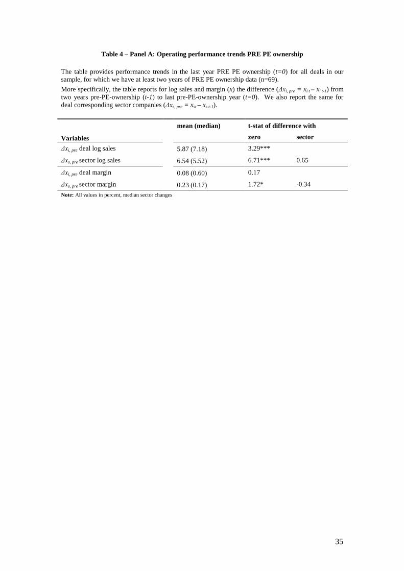
Table 4, Panel A provides a snapshot of the operating performance change for the

deals in our sample prior to acquisition and hence, for the three operating measures (x),

reports: the difference (Δxi, pre = xi t - xi t-1) from two years before PE ownership (t-1) to last the

pre-acquisition year (t). We also show these figures for the corresponding sector companies

(Δxs, pre = xs t - xs t-1) and use median sector changes, given that there are generally fewer than

100 companies in each three digit, ICB sector. As described in Kaplan (1989), and also

according to the deals in our sample with sufficient operational data available (n=69), PE does

not seem to pick companies that were exposed to a negative idiosyncratic shock, which in

better times would revert to the mean, potentially allowing the target to be sold with an

upside. Target companies show a robust pre-acquisition increase in nominal sales, together

with constant profitability. Importantly, in terms of performance trends, PE owned companies

do not differ in a statistically significant way from their sector peers in the pre-acquisition

phase.

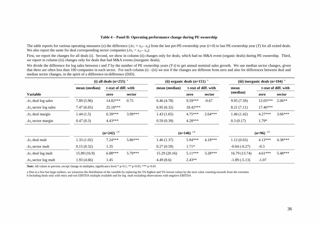
Table 4, Panel B captures the change during PE ownership and shows the difference

(Δxi = xiT - xit) from the last pre-acquisition year (t) to the last PE-ownership year (T);.we

analyse the annual change by dividing the difference, Δxi, by the number of years of PE

ownership (T-t).

20

In the first set of columns, we report the changes for all deals with sufficient

operational data available (n=255). In the second and third column, we separate deals with

organic strategies (n=151) from those with inorganic strategies (n=104), the latter of which

include major, follow-on M&A events during the private phase, so that we can analyze Δxi by

strategy. This also allows us to control for the effects of M&A events, which cause sales to

increase, and EBITDA margin and multiple to either increase or decrease, subject to the ratios

of the acquired entity. It is important to note that the first M&A event tends to happen after

one year, on average, for deals in the McKinsey sample (for which detailed information on

M&A events is available) – this tends to suggest that, given the planning required to execute

an acquisition, M&A events are planned rather than a reaction to better- or worse-than

anticipated performance.

We also test if the changes are different from zero and, in the spirit of a difference-in-

difference (DiD), also test for differences between deal and median sector changes.

Overall, PE ownership tends to have a positive impact on the operating performance

in our sample. As shown in Table 4, Panel B, column (i) on average, all deals show a margin

improvement of 1% and a multiple improvement of 1.1 during PE ownership, relative to their

sector peers. Interestingly, the margin improvements of the deals in our sample are slightly

lower than the 1.4%-3.8% reported in Kaplan (1989). In contrast, deals do not outperform the

sector in terms of annual sales growth, although portfolio company sales do grow by a

statistically significant 7.9% during PE ownership.

Another important result of Table 4, Panel B is that large M&A transactions do not

cause our findings on underlying operating improvements to change: separately, both origanic

and inorganic deals, columns (ii) and (iii) respectively, display improvements in both

EBITDA margin and multiple, relative to their sector peers.14

14 In a robustness check in the McKinsey data set, we also include deals with M&A events after 2 years of PE ownership in the organic deal set and find our results qualitatively unchanged. We include those deals, since late M&A events might be endogenously determined by the observed performance of the deal. M&A events in the first 2 years can be treated as “exogenous”, if we assume that it takes at least one year to find out that a deal is underperforming and at least another year to identify and buy another company.

Only inorganic deals seem to

21

increase sales above sector, but this isn’t surprising due to the large, post-deal M&A

transactions involved which naturally boost revenue.

6. Abnormal performance and operating performance

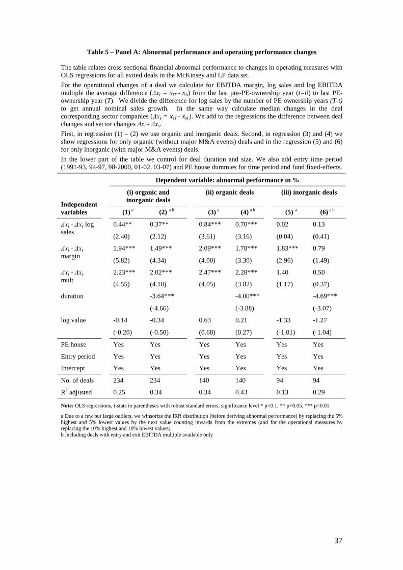
Having separately identified abnormal financial and operating performance of PE

deals relative to quoted peers, we investigate the relationship between the two measures in

Table 5, Panel A. Specifically, we regress abnormal performance on the increase in EBITDA

margin, growth in sales and change in EBITDA multiple. Columns (1) and (2) present results

for the whole sample but once more we distinguish between organic (Columns 3 and 4) and

inorganic deals (Columns 5 and 6). We also control for duration and deal size at entry date,

and include dummies for different entry time periods and PE houses, in order to control for

time and the fixed effects of PE firms on their acquisitions.15

Of the three measures of operating performance, the two which we identified as being

improved during PE ownership – EBITDA margin and multiple – also appear to be significant

determinants of abnormal performance: changes in either measure have a positive and

economically meaningful impact on abnormal performance (Columns 1 and 2). Sales growth,

also relates to abnormal performance, even though it is not improved by PE in general above

sector (as shown previously in Table 4, Panel B),

Another potential driver of

abnormal performance is that PE houses may have been lucky on some deals simply because

they bought them at the right time when the margins or multiples in the sector were growing.

We therefore include the change above sector for all three operating measures.

For organic deals, Table 5, panel A, regression (3), abnormal performance is driven

by changes in all three operating measures: a 1% improvement in EBITDA margin above

sector increases abnormal performance by roughly 2.1%; a growth of the multiple from entry

to exit by 1 increases abnormal performance by roughly 2.5%; and a 1% sales growth above

15 However, in unreported results, we find that the significance and size of the estimates on operating improvements is minimally affected by omitting time dummies for entry years. We do not include dummies for the size of the deals since size does not show up as significant and does not increase the explanatory power. This is potentially due to a lack of variation in size in our sample that consists solely of large deals.

22

sector alters abnormal performance by 0.8%. Our results are qualitatively unchanged when

we include duration in the regression in column (4). For inorganic deals, however, there is

little evidence to suggest that changes in operational performance drive abnormal

performance: only margin improvements seem to contribute to abnormal performance

(although the size and significance is lower than for organic deals), but the result is

inconclusive, as deals with significant, follow-on M&A are subject to an error term due to

distortion by the acquired entity.

The economic contribution of these operating improvements is substantial in

explaining abnormal performance. In the previous sections we identified a median abnormal

performance of 15.4% for all deals (Table 3, Panel A) and, for organic deals, a typical

EBITDA margin increase of circa 1% and a multiple increase of circa 1 above sector (Table

4, Panel B(ii)). Based on the estimated coefficients in regression (3), operational performance

changes explain nearly one third of the abnormal performance (4.6/15.4).

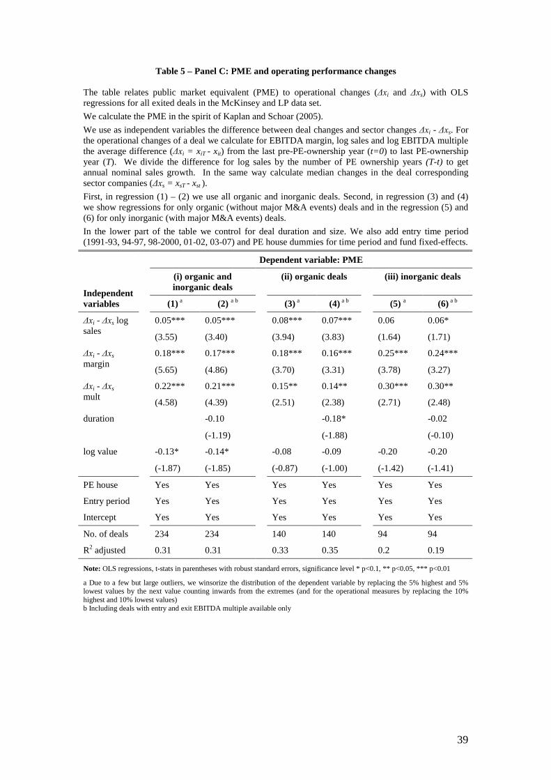
Our findings are also robust to alternative measures of financial performance. In

Table 5, Panel B, we simply replace the dependent variable abnormal performance with IRR

and, in Panel C with, PME based on sector. In Panel C, regression (3), margin, multiple and

sales improvements above sector are significant explanatory factors of PME based on sector.

We conclude that operational improvements explain abnormal performance and distinguish

good deals from others in terms of financial value creation. This is a potentially important

result: it provides insight that operating value creation strategies might be at play in different

PE deals, as we explore below.

7. Human capital factors of deal partners

7.1. Financial performance and deal partner background

We now show that the “fit” between a deal partner’s background (professional

experience in finance vs. operations) and deal strategy (organic vs. inorganic) correlates with

deal performance. This could be considered as evidence that task-specific skills of the PE

23

partners are relevant to deal performance. We follow the simple, but plausible idea of

Gibbons and Waldman (2004) that mainly task-specific learning-by-doing leads to an

accumulation of human capital. In particular, in our case we hypothesize that deal partners

with financial backgrounds have learned skills via investment banking activities, or similar,

and those with operational backgrounds have learned revenue growth and cost-cutting skills

by undertaking these activities in their previous jobs. Further, if this is true, then more

partners with financial backgrounds should be matched to deals with M&A activity, and

partners with operational backgrounds should be matched to organic deals, assuming that PE

firms match the skills of their partners to the needs of their deals.

For the LP data, we identify the leading deal partner as the partner first mentioned in

the execution of the deal. For the McKinsey data, we base our analysis on additional deal-

level information, collected through interviews with general partners (GPs). We interviewed

72 deal partners involved in our deals16

16 We verified if the interviewee was indeed the single leading partner for the deal with information from the Capital IQ database, the PE house website, or press articles. We had to change the background for only a few deals, since another single leading deal partner with a different background from the interviewee was mentioned.

; for an additional 30 deals where no interview was

available, we identified the leading deal partner from a number of sources, including Capital

IQ, PE house websites, or press articles. We used the same three sources to identify the

professional backgrounds (either operational, including industry or management consulting

experience, or not – the latter typically including investment bankers and accountants); their

education (science background, MBA, Charted Accountant); and experience in the PE

industry (number of years in the PE industry at deal entry date). To verify the

representativeness of our sample of deal-partners, we gathered information on the

professional backgrounds for additional deal partners from 200 randomly drawn PE

investments made by funds having a similar size as the funds in our sample and found that the

share of operating versus non-operating partners was not significantly different from our

sample (non-tabulated results).

24

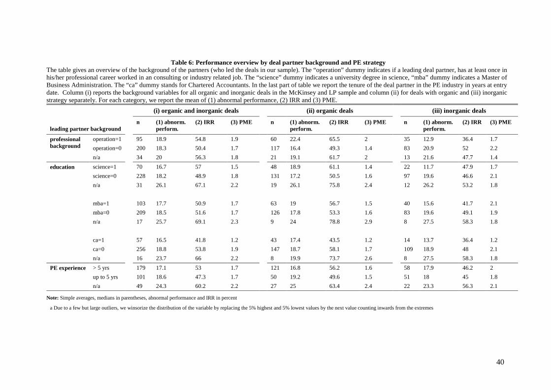
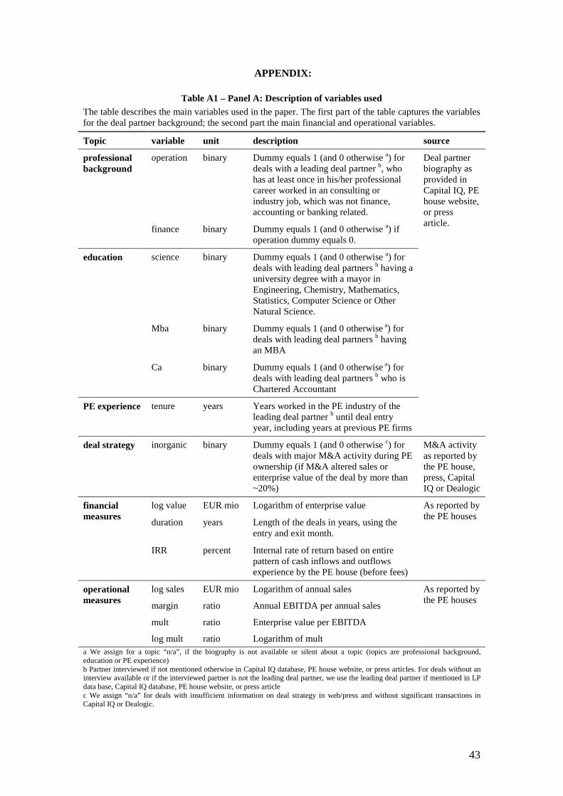
Table 6 gives an overview of the partners’ backgrounds and their performance by

deal strategy. For each deal partner, we assign dummy variables for their professional

background, education, and experience (for a detailed description of the variables see Table

A1 in the appendix). The operation dummy records whether a leading deal partner has ever

worked in consulting or industry – which is the case for only one-third of the leading deal

partners (95 out of 295); most leading deal partners are pure bankers or accountants. For

organic deals, operating partners generate higher abnormal performance on average (22.4%)

compared to non-operating (finance) partners (16.4%); the reverse is true for inorganic deals,

where operating partners generate lower abnormal performance (12.9%) compared to non-

operating partners (20.9%). The same observations are true for IRR and PME. We also

observe, from the ratio of partner backgrounds by deal strategy, that PE firms appear, on

average, to do little, if any, skill-matching: in our sample, 34% (60/177) of partners assigned

to organic deals have operating backgrounds, but 30% (35/118) of partners assigned to

inorganic deals have operating backgrounds too. More generally, to examine the deal partner

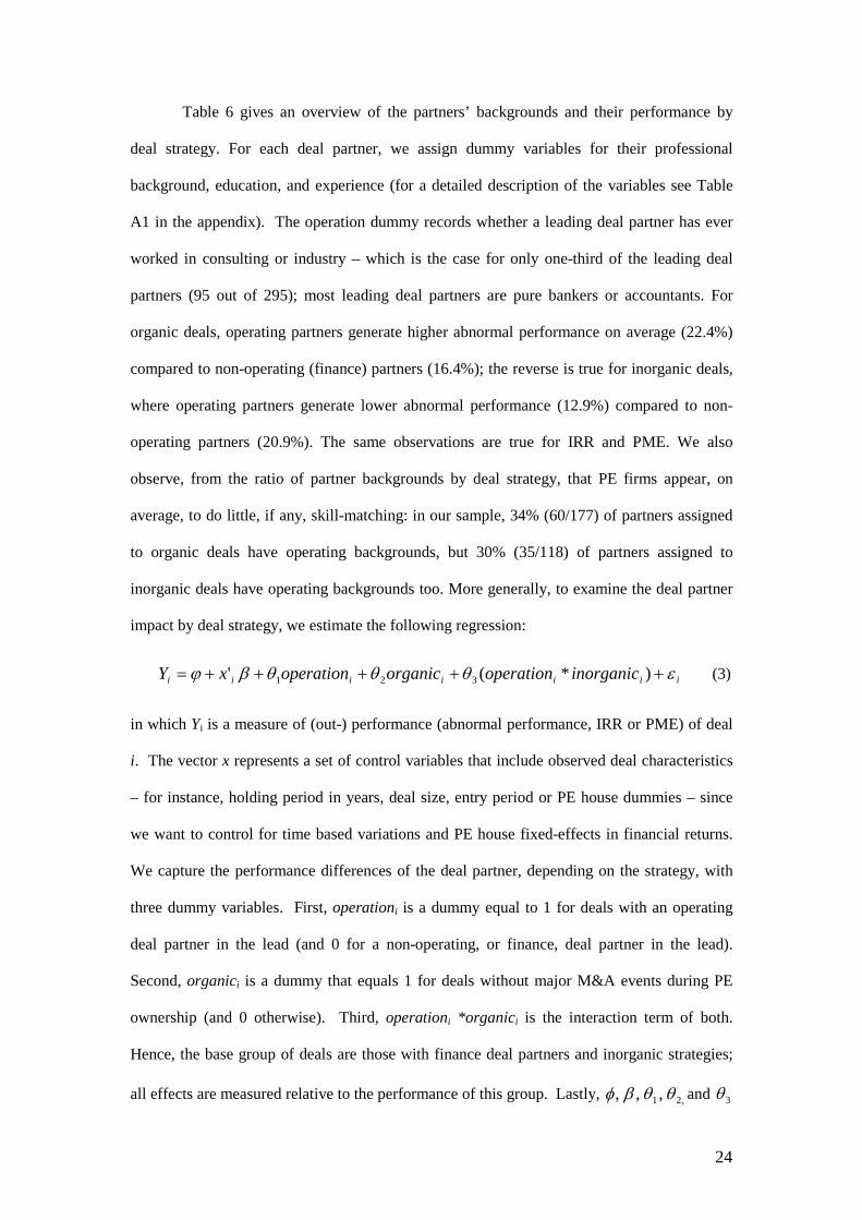
impact by deal strategy, we estimate the following regression:

iiiiiii inorganicoperationorganicoperationxY εθθθβϕ +++++= )*(' 321 (3)

in which Yi is a measure of (out-) performance (abnormal performance, IRR or PME) of deal

i. The vector x represents a set of control variables that include observed deal characteristics

– for instance, holding period in years, deal size, entry period or PE house dummies – since

we want to control for time based variations and PE house fixed-effects in financial returns.

We capture the performance differences of the deal partner, depending on the strategy, with

three dummy variables. First, operationi is a dummy equal to 1 for deals with an operating

deal partner in the lead (and 0 for a non-operating, or finance, deal partner in the lead).

Second, organici is a dummy that equals 1 for deals without major M&A events during PE

ownership (and 0 otherwise). Third, operationi *organici is the interaction term of both.

Hence, the base group of deals are those with finance deal partners and inorganic strategies;

all effects are measured relative to the performance of this group. Lastly, ,21 ,,, θθβφ and 3θ

25

are coefficients to be estimated and iε is the regression error. The coefficients are estimated

by cross-sectional variation, since we have only one observation of Y per deal.

In Table 7 we provide evidence that the success of operating or finance deal partners

depends on the deal strategy – something alluded to in Table 6. Operating partners outperform

for organic strategies, whereas finance partners outperform for inorganic strategies. This

finding is qualitatively robust to alternative specifications, in particular to alternative

measures of outperformance, including IRR or PME. In regressions (1)-(4) we also include

duration as an explanatory variable. However, since duration might be determined by deal

performance, we show the same in regressions in (5)-(8) without controlling for this variable.

First, in regressions (1) and (5), when we only add operationi, it is not clear if

operating partners in general under- (1) or out-perform (5) relative to non-operating partners –

the coefficients are both small and statistically insignificant; the same is true for regressions

(2) and (6), when we add the term organici. Only in regressions (3) and (7), when we add

organici and the interaction term operationi *organici – in order to control for partner

background effects that are strategy specific – do we get a statistically significant finding. On

the basis of (7), we conclude that operating partners outperform the base group for organic

strategies (by 14.4%) and underperform for inorganic strategies (by 9.1%). In regressions (4)

and (8) we control for other variables of deal partner background and find our results

qualitatively unchanged, although larger in magnitude.

In Table 8, regressions (1)-(2), we confirm that our findings are robust to alternative

measures of performance, using IRR or PME as the dependent variable instead of abnormal

performance and the same independent variables as in regression (8), Table 7. Both

regressions (1)-(2) show the same sign and similar significance for the interaction term

operationi *organici. We also check that the outperformance of operating or finance partners

does not seem to be caused by sector-picking abilities. In regressions (3)-(4) we use levered

and un-levered sector returns as the dependent variables and do not find any statistically

significant relationship between partner background, strategy and returns. Whilst we already

26

control for leverage and sector returns in abnormal performance, this serves as a more direct

test, ruling out the contribution of sector-picking to our results, linking deal partner

background to deal performance. Note, however, that organic strategies appear to be linked

with relatively high sector returns, which tends to suggest that organic strategies are pursued

in high-growth sectors. According to regression (5), deal leverage is not explained by deal

strategy or partner background. In regressions (6)-(8) we replace abnormal performance as

the dependent variable with sales growth, margin and multiple improvements above sector

respectively, to see if there are operational performance differences by partner background.

The significance of the interaction term operationi *organici in regression (7) bolsters our

findings: operating deal partners seem to improve margins by 2.6% more in organic deals

than non-operating partners.

Overall, these results expand the already established facts found in the VC literature

to the PE industry: We show that prior business experience is relevant for PE fund

investments in a manner that seems to suggest investor activism. In line with findings of

Bottazzi et al. (2008) for the VC industry, we hypothesize that deal partners frequently

interact with the portfolio company to shape its organic or M&A strategy. Since returns to

such skills gathered over time are not found for mutual fund managers (Chevalier and Ellison,

1999), it seems that PE funds are more similar to VC in this regard than mutual fund

investments.

8. Concluding remarks

The surge in PE funding from 2003 through to the middle of 2007, and the aftermath

of the sub-prime crisis since then, has caused research on PE to confront similar issues as

those after the boom and bust cycles of the late 80s and early 90s. Significant policy interest

has also been expressed in understanding and quantifying the long-run impact of PE in terms

27

of value creation at the enterprise level, and in the attribution of this value creation to

financial engineering, systematic risk and operational engineering.17

This paper is best viewed as an attempt to get at some of these issues with three

significant contributions. First, we provide a simple methodology that relies only on returns

and leverage information at the level of deal’s equity, and the returns and leverage of quoted

peer firms, in order to extract a measure of abnormal performance of the deal at enterprise-

level. The methodology also quantifies the sector and leverage contributions to deal return.

Second, by using this measure of abnormal performance we show that for deals of large,

mature PE houses in Western Europe, there is evidence consistent with value creation for

portfolio companies on average. Furthermore, abnormal performance correlates well with

operating outperformance of deals measured as improvement in EBITDA margins and

multiples relative to the quoted sector. Third, we provide evidence that the superior

performance of these PE houses is at least partly due to differences in human capital factors.

In particular, the match between the deal strategy (M&A-based or organic) and deal partner

background (financial/accounting or operating/consulting) is correlated with deal

performance.

Overall, our results can be interpreted as providing a microscopic view on the

operational expertise employed by large, mature PE houses in improving companies they

acquire. Returns to this expertise are likely the reason behind persistent and significant out-

performance of funds run by these houses.

References Acharya, V., J. Franks and H. Servaes. 2007. Private Equity: Boom and Bust? Journal of Applied Corporate Finance, 19(4), 44-53. Acharya, V., C. Kehoe and M. Reyner,. 2009. Private Equity Vs. PLC Boards in the U.K.: A Comparison of Practices and Effectiveness. Journal of Applied Corporate Finance, Vol. 21, Issue 1, pp. 45-56,

17 Indeed, in some cases such as in the UK, policymakers have undertaken independent recommendations based on interactions with the PE industry to improve disclosure on such value attribution. See the House of Commons Treasury Committee’s Tenth Report in the UK of Session 2006-07 and Sir David Walker Report on “Disclosure and Transparency in Private Equity” (2007).

28

Axelson, U., P. Stromberg and M. Weisbach 2009. The Financial Structure of Private Equity Funds. Journal of Finance, 64(4), 1549-1582. Axelson, U., T. J. Jenkinson, P. Stromberg, and M. Weisbach. 2008. Leverage and Pricing in Buyouts: An Empirical Analysis. Working Paper, Swedish Institute for Financial Research. Bottazzi, L., Rin, M., and T. Hellmann. 2008. Who are the active investors? Evidence from venture capital. Journal of Financial Economics 89 (2008) 488-512. Carhart, M. 1997. On Persistence in Mutual Fund Performance. Journal of Finance, 52(1), 57-82. Chevalier, J., and G. Ellison. 1999. Are Some Mutual Fund Managers Better than Others? Cross-Sectional Patterns in Behavior and Performance. Journal of Finance, pp. 875-899. Cumming, D., S. D. Siegel, and M. Wright. 2007. Private Equity, Leveraged Buyouts and Governance. Journal of Corporate Finance 13 (2007) 439–460. Dimov, S., and D. Shepherd. 2005. Human Capital Theory and Venture Capital Firms: exploring”home runs” and “strike outs”. Journal of Business Venturing, 20 (2005) 1-21. Gibbons, R., and M. Waldman. 2004. Task-Specific Human Capital. American Economic Review, Vol. 94(2), pp. 203-207. Groh, A. P. and O. Gottschalg. 2011. The effect of leverage on the cost of capital of US buyouts. Journal of Banking and Finance. Forthcoming Guo, S., E. S. Hotchkiss, and W. Song. 2011. Do Buyouts (Still) Create Value. Journal of Finance, 66, 479-517. Harris, R., S. D. Siegel and M. Wright. 2005. Assessing the Impact of Management Buyouts on Economic Efficiency: Plant-Level Evidence from the United Kingdom. Review of Economic and Statistics, Vol.87, pp. 148-153. Hellmann, T., and M. Puri. 2002. Venture capital and the professionalization of start-ups: Empirical Evidence. Journal of Finance, Vol. 57, pp. 169–197. Jensen, M. 1989. Eclipse of the Public Corporation. Harvard Business Review, Sept.-Oct., 61-74. Jones, C. M. and M. Rhodes-Kropf. 2003. The Price of Diversifiable Risk in Venture Capital and Private Equity. AFA 2003 Washington, DC Meetings. Kaplan, S. 1989. The Effects of Management Buyouts on Operations and Value. Journal of Financial Economics 24, 217-254. Kaplan, S. and A. Schoar. 2005. Private Equity Performance: Returns, Persistence, and Capital Flows. Journal of Finance, vol. 60, no. 4 (August):1791–1823. Kaplan, S. and J. Stein. 1993. The Evolution of Buyout Pricing and Financial Structure in the 1980s. Quarterly Journal of Economics, Volume 108, May, 1993, 313-358. Kaplan, S. and P. Stromberg. 2008. Leveraged Buyouts and Private Equity. Journal of Economic Perspectives. Vol. 23, issue 1, pages 121-46.

29

Kaplan, S., N., Klebanov, M. Mark and M. Sorensen. 2008. Which CEO Characteristics and Abilities Matter? AFA 2008, New Orleans Meetings Paper, July 2008. Lerner, J., and A. Schoar. 2004. The Illiquidity Puzzle: Theory and Evidence from Private Equity. Journal of Financial Economics, vol. 72, no. 1 (April):3–40. Lerner, J., A. Schoar, and W. Wong. 2007. Smart Institutions, Foolish Choices? The Limited Partner Performance Puzzle. Journal of Finance. Vol. 62(2), pages 731-764. Lerner, J., M. Sorensen, and P. Stromberg. 2008. Private Equity and Long-Run Investment: The Case of Innovation. Working Paper, Stockholm School of Economics. Leslie, P. and P. Oyer. 2008. Managerial Incentives and Value Creation: Evidence form Private Equity. Working Paper, Stanford-GSB. Lichtenberg, F. and D. S. Siegel. 1990. The Effects of Leveraged Buyouts on Productivity and Related Aspects of Firm Behaviour. Journal of Financial Economics. Vol. 27 (1990) 165-194. Ljunqvist, A., M. Richardson and D. Wolfenzon. 2007. The Investment Behavior of Buyout Funds: Theory and Evidence. Working Paper, Stern School of Business, New York University. Metrick, A. and A. Yasuda. 2007. Economics of Private Equity Funds, Working Paper, Wharton Business School. Nikoskelainen, E. and M. Wright. 2007. The impact of corporate governance mechanisms on value increase in leveraged buyouts. Journal of Corporate Finance. Vol. 13(4), pages 511-537, September. Palepu, K. G. 1990. Consequences of Leveraged Buyouts. Journal of Financial Economics 27, 247-262. Phalippou, L. 2007. Investing in Private Equity Funds: A Survey. Working Paper, University of Amsterdam. Phalippou, L., and O. Gottschalg. 2009. The Performance of Private Equity Funds. Review of Financial Studies, 22(4):1747-1776.. Renneboog, L., T. Simons, and M. Wright. 2007. Why do firms go private in the UK? Journal of Corporate Finance, 13(4), 591-628. Smith, A. 1990. Corporate ownership structure and performance: The case of management buyouts. Journal of Financial Economics, Vol. 27 (1990) 143-164. Zarutskie, Rebecca. 2010. The role of top management team human capital in venture capital markets: Evidence from first time funds. Journal of Business Venturing, Vol. 25 (2010), pp. 155-172.

Table 1 – Panel A: Distribution of deals by entry and exit years The table shows the years in which the PE houses bought (entry) or sold (exit) the portfolio companies (deals) in the McKinsey and LP data set (our sample). a

Years 1991 92 93 94 95 96 97 98 99

Entry 3 2 2 1 3 23 34 42 44

Exit 2 2 3 8 12

2000 1 2 3 4 5 6 7 2008 SUM

Entry 38 46 54 45 28 20 8 2 395

Exit 14 21 19 36 54 71 64 70 a 19 395

a Including six deals for which exit is simulated

Table 1 – Panel B: Summary statistics The table shows various financial measures for the deals in the McKinsey and LP data set. The first part reports the financial performance and the duration. We calculate the deal IRRs (internal rate of return) using the entire time pattern of cash inflows and outflows for each deal (portfolio company), as experienced by the PE house (before fees). The cash in/cash out multiple measures the absolute value of all positive cash flows divided by all negative cash flows minus 1. The duration captures the length of the deals in years, using the entry and exit months and years as reported by the PE house. The second part of the table compares the enterprise value (deal size) and several financial ratios between entry and exit date. The number of observations is smaller than in the first part, since we only include deals that the PE funds sold, and have to exclude deals with an equity value of zero. In addition, information on EBITDA at entry and exit is not available for all deals. In the last column we test for differences between exit and entry values.

Variable n mean (median) std. dev. min max t-stat of diff. exit and entry

deal IRR (gross) % a 395

56.1 (43.2) 46.6 0.0 179.0

cash in/cash out multiple 4.4 (3) 9.5 0.0 130.0

duration (years) b 385 3.9 (3.4) 2 0.4 10.8

deal size (entry) b 385

430.2 (141.2) 756.8 0.0 6485.6 8.48***

deal size (exit) b 749.6 (244) 1311.9 0.0 10290.0

debt/equity (entry) a b 381

2.2 (1.9) 1.5 0.3 6.2 -15.18***

debt/equity (exit) a b 0.8 (0.5) 0.9 0.1 3.8

mult (entry) c 354

6.8 (6.5) 11.1 -173.3 42.9 2.91**

mult (exit) c 8.6 (7.9) 7.5 -67.4 54.5

debt/EBITDA (entry) c 354

4.1 (4.1) 6.9 -104.7 35.9 -3.37***

debt/EBITDA (exit) c 3.0 (2.5) 3.1 -13.2 21.7 Note: In Mio EUR; significance level * p<0.1, ** p<0.05, *** p<0.01

a Due to a few but large outliers, we winsorize the distribution of the variable by replacing the 5% highest and 5% lowest values by the next value counting inwards from the extremes b Only exited deals c Only exited deals and if EBITDA for exit and entry date is available

31

Table 2 – Panel A: Benchmarking of our funds vs. PE universe funds This table compares the returns and size of the funds in the McKinsey and LP data set (our sample) with fund returns and size of the PE universe as reported in Preqin. First, row (1) reports the net IRR and fund size for 48 (out of 84 a) funds which participate in our sample and for which Preqin reports net IRRs. Second, we provide net IRRs and fund size for the PE universe in Western Europe (with the same vintage years as the funds in our sample) as reported in Preqin. Row (2) shows the net IRRs for all funds in Western Europe and (3) for large funds only. We further test if the PE funds in our sample are different in terms of net IRR and fund size from (2) the Western European universe and (3) the universe with similar fund size (above USD 300 mio fund size, since only 5 of the funds in our sample are smaller). Net IRR, in % fund size, in Mio EUR

n

mean (median) t-stat of diff. with (1)

mean (median) t-stat of diff. with (1)

(1) Our funds 48 24.88 (21.75) 1567.05 (920)

(2) Funds in PE universe 146 23.53 (20.45) -0.41 700.76 (248.29) -4.43***

(3) Large funds in PE universe b

78 22.28 (19.75) -0.44 1402.4 (787.96) -0.89

Note: Vintage year 1991-2005, significance level * p<0.1, ** p<0.05, *** p<0.01

a In 5 cases, more than one fund of a PE house is involved; in these cases we take the simple average fund net IRR of the funds involved and treat the funds as one fund b Funds larger than USD 300 mio fund size

32

Table 2 – Panel B: Benchmarking of deals vs. fund returns in McKinsey data set This table compares the deals with the funds in the McKinsey sample by net IRRs. Row (1) provides the net IRR for 32 out of 36 funds that participate in our sample and for which Preqin reports the net IRRs by end of 2007. In row (2) we show the simple average net IRRs of all deals in the McKinsey sample for which we have publicly available fund return data (for 93 out of 110 deals in the McKinsey sample). In row (3) we pool these deals artificially in one pseudo fund. Since the data on the European universe is primarily in the form of net IRRs, we convert our gross deal-level IRRs (before fees charged by PE houses to fund investors) to net IRRs (after fees, or in other words, IRRs from the viewpoint of fund investors). In the last column we test if the PE houses cherry-picked the deals in (2) out of their funds (1) in terms of performance. Net IRR a, in %

n mean (median) t-stat of

difference

(1) Our funds b 32 28.13 (26.38)

(2) Our deals 93 26.25 (25.02) -0.43 c

(3) Our deals pooled in 1 pseudo fund d 1 23.91% Note: Vintage year 1993-2003, significance level * p<0.1, ** p<0.05, *** p<0.01

a Net IRR, estimated for our deals in the following way: If a) gross IRR<=10%, then LPs keep all return except 2% fees, so that net IRR = gross IRR - 2% fees; b) 10%<gross IRR<12.5%, then LPs keep all return up to 10% except for 2% fees and GPs keep all return from 10% to 12.5%, so that net IRR = gross IRR - 2% fees – (gross IRR – 10)% = 8%; and c) gross IRR>=12.5%, then LPs and GPs share in 80:20 ratio the return exceeding 12.5%, so that net IRR = gross IRR - 2% fees – 2.5% - 20%*(gross IRR - 12.5%) b In 5 cases, more than one fund of a PE house is involved; in these cases we take the simple average fund net IRR of the funds involved and treat the funds as one fund. For 1 deal the fund names is unknown, for 3 funds we cannot find fund returns c Assuming unequal variance for (1) and (2) d Pooled by calendar period using quarterly cash flows.

Table 2 – Panel C: Benchmarking of deals used from LP data set

This table compares net IRRs and deal size of (1) the deals from the LP data set used in the analyses with (2) the deals from the LP data set not used in the analysis (but which are from the same PE houses and for which information on IRR and size was available). We exclude deals in (2) from the analyses, due to missing information, e.g., on leverage or deal partner names. In the first column we test if (1) and (2) are different by IRR and in the last column if (1) and (2) are different by deal size. IRR, in % deal size, in Mio EUR

n mean (median) t-stat of

diff. a mean (median) t-stat of

diff. a

(1) Deals from LP data set used

285 91.6 (47.75) % -0. 42 372.49 (106.505)

0.35

(2) Deals from LP data set not used b

892 104.2 (40.99) % 350.74 (85.0)

Note: Significance level * p<0.1, ** p<0.05, *** p<0.01 a Assuming unequal variance for (1) and (2) b Deals with information on IRR (n=671) or deal value available (n=342)

33

Table 3 – Panel A: IRR decomposition The table provides simple averages of three gross IRR components: (i) Deal-level abnormal performance (alpha): αi measures the excess asset return generated at the enterprise level of the portfolio company for PE investors. It is purged of the effect of leverage financing the firm takes on, since αi = RUi - RSUi . Whereby RUi is the un-levered return of the deal i and RSUi the un-levered return of the sector i, using the standard un-levering formula. a b (ii) Levered sector return: RSUi (1+D/ESi) - RDi (1-t)(D/ESi) measures the effect of contemporaneous sector returns, including the effect of sector-level leverage. For the sector, we use the median IRR in each deal corresponding sector. (iii) Return from incremental leverage: (RSUi - RDi (1-t))(D/Ei-D/ESi)+αi(D/Ei) captures the amplification effect that a) the incremental deal leverage beyond the sector leverage, (D/Ei-D/ESi) has on the sector returns and b) the total leverage has on enterprise-level out-performance. We report the IRR decomposition for different scenarios: (1) We break down the returns for all deals, (2)-(6) for the deals separately by entry year, and (7) only for deals for which the cost of debt was available. Scenario n (i) deal-level

abnormal performance

(ii) levered sector return

(iii) return from incremental leverage

total IRR c Abnormal perfor-mance per IRR

(1) All deals 395 19.8 (15.4) 8.5 (8.4) 27.9 (19.1) 56.1 (43.2) 33.93%

(2) 1991-93 7 32.2 (28.5) 9.8 (9.1) 29.1 (26.4) 71.1 (70.9) 45.07%

(3) 1994-97 61 20.5 (13.8) 8.5 (7) 30.4 (19.7) 59.4 (41.9) 33.90%

(4) 1998-00 124 16.5 (12) 0.7 (1.5) 18 (12) 35.2 (25) 45.71%

(5) 2001-02 100 17.5 (14.6) 11.2 (12.1) 21.9 (17.9) 50.6 (42.9) 34.00%

(6) 2003-07 103 24.7 (21.8) 15 (16.1) 43.9 (36.6) 83.5 (73.3) 28.92%

(7) Deals with cost of debt information 67 11 (10.1) 11.2 (10.1) 20.7 (15.2) 42.8 (40) 26.19% Note: All values in percent, simple averages, medians in parentheses a We further use the average D/E ratio during deal life for the deals, a median D/E ratio over 3 year for the sector and β=1. We further assume the same cost of debt and corporate tax rate for the sector as for the deal b Out of the 110 deals in the McKinsey data set, we find for 62 deals the cost of debt (based rate and margin spread) in Dealogic; for 15 we only find the base rate (Libor vs. Euribor); and for 23 deals we find no information. If the margin spread is unknown for a deal we use the median spread of PE deals in Western Europe in the same year. If the base rate is unknown we use Libor for UK deals and Euribor for all other deals. For the 285 deals from the LP data set we assume an average cost of debt of 7% and 30% corporate tax rate c Due to a few but large outliers, we winsorize the IRR distribution by replacing the 5% highest and 5% lowest values by the next value counting inwards from the extremes

34

Table 3 – Panel B: Abnormal performance, IRR vs. PME The table reports for all deals in the McKinsey and LP data set (our sample) summary statistics on (1) abnormal performance, (2) IRR and (3) the public market equivalent (PME) for each deal in the spirit of Kaplan and Schoar 2005. In the PME calculation, we discount all cash flows with the total sector return and then calculate the ratio of discounted cash flows to the largest cash inflow for the deal.

Performance measure n a mean (median) std. dev. min max

(1) Abnormal performance

395

19.8 (15.37) 22.88 -22.87 145.63

(2) IRR gross 56.1 (43.18) 46.62 0 179.05

(3) PME Sector 1.88 (1.37) 1.87 -0.16 7.17

a Due to a few but large outliers, we winsorize the IRR and PME distribution by replacing the 5% highest and 5% lowest values by the next value counting inwards from the extremes

Table 3 – Panel C: Correlation matrix: Abnormal performance, IRR, PME and sector returns

The table shows for all deals in the McKinsey and LP sample (n=395) a the correlation between abnormal performance (scenario 1), IRR, the public market equivalent (PME), levered and un-levered median sector returns.

IRR gross PME Sector Levered sector return

Abnormal performance 0.73*** 0.53*** -0.28***

PME Sector 0.53*** 1 -0.32*

Levered sector return 0.17*** -0.32*** 1 Note: All values in percent, significance level (of the pairwise correlation coefficient) * p<0.1, ** p<0.05, *** p<0.01

a Due to a few but large outliers, we winsorize the IRR and PME distribution by replacing the 5% highest and 5% lowest values by the next value counting inwards from the extremes

35

Table 4 – Panel A: Operating performance trends PRE PE ownership The table provides performance trends in the last year PRE PE ownership (t=0) for all deals in our sample, for which we have at least two years of PRE PE ownership data (n=69). More specifically, the table reports for log sales and margin (x) the difference (Δxi, pre = xi t – xi t-1) from two years pre-PE-ownership (t-1) to last pre-PE-ownership year (t=0). We also report the same for deal corresponding sector companies (Δxs, pre = xst – xs t-1).

Variables

mean (median) t-stat of difference with zero sector

Δxi, pre deal log sales 5.87 (7.18) 3.29***

Δxs, pre sector log sales 6.54 (5.52) 6.71*** 0.65

Δxi, pre deal margin 0.08 (0.60) 0.17

Δxs, pre sector margin 0.23 (0.17) 1.72* -0.34 Note: All values in percent, median sector changes

36

Table 4 – Panel B: Operating performance change during PE ownership The table reports for various operating measures (x) the difference (Δxi = xiT - xit) from the last pre-PE-ownership year (t=0) to last PE-ownership year (T) for all exited deals. We also report the same for deal corresponding sector companies (Δxs = xsT - xst). First, we report the changes for all deals (i). Second, we show in column (ii) changes only for deals, which had no M&A event (organic deals) during PE ownership. Third, we report in column (iii) changes only for deals that had M&A events (inorganic deals). We divide the difference for log sales between t and T by the number of PE ownership years (T-t) to get annual nominal sales growth. We use median sector changes, given that there are often less than 100 companies in each sector. For each column (i) - (iii) we test if the changes are different from zero and also for differences between deal and median sector changes, in the spirit of a difference-in-difference (DiD).

a Due to a few but large outliers, we winsorize the distribution of the variable by replacing the 5% highest and 5% lowest values by the next value counting inwards from the extremes b Including deals only with entry and exit EBITDA multiple available and for log mult excluding observations with negative EBITDA

Variable

(i) all deals (n=255) a (ii) organic deals (n=151) a (iii) inorganic deals (n=104) a

mean (median) t-stat of diff. with mean (median) t-stat of diff. with mean (median)

t-stat of diff. with

zero sector zero sector zero sector

Δxi deal log sales 7.89 (5.96) 14.82*** 0.75 6.46 (4.78) 9.59*** -0.67 9.95 (7.59) 12.05*** 2.06**

Δxs sector log sales 7.47 (6.65) 25.18*** 6.95 (6.32) 18.42*** 8.21 (7.11) 17.46***

Δxi deal margin 1.44 (1.5) 6.39*** 3.99*** 1.43 (1.65) 4.75*** 2.64*** 1.46 (1.42) 4.27*** 3.06***

Δxs sector margin 0.47 (0.3) 4.43*** 0.59 (0.39) 4.28*** 0.3 (0.17) 1.79*

(n=242) a b (n=146) a b (n=96) a b

Δxi deal mult 1.33 (1.02) 7.24*** 5.86*** 1.46 (1.37) 5.94*** 4.18*** 1.12 (0.63) 4.13*** 4.38***

Δxs sector mult 0.15 (0.32) 1.35 0.27 (0.59) 1.71* -0.04 (-0.27) -0.3

Δxi deal log mult 15.89 (16.9) 6.88*** 5.79*** 15.29 (20.16) 5.11*** 3.28*** 16.79 (13.74) 4.61*** 5.48***

Δxs sector log mult 1.93 (4.66) 1.45 4.49 (8.6) 2.43** -1.89 (-5.13) -1.07 Note: All values in percent, except change in multiples, significance level * p<0.1, ** p<0.05, *** p<0.01

37

Table 5 – Panel A: Abnormal performance and operating performance changes

The table relates cross-sectional financial abnormal performance to changes in operating measures with OLS regressions for all exited deals in the McKinsey and LP data set. For the operational changes of a deal we calculate for EBITDA margin, log sales and log EBITDA multiple the average difference (Δxi = xiT - xit) from the last pre-PE-ownership year (t=0) to last PE-ownership year (T). We divide the difference for log sales by the number of PE ownership years (T-t) to get annual nominal sales growth. In the same way calculate median changes in the deal corresponding sector companies (Δxs = xsT - xst ). We add to the regressions the difference between deal changes and sector changes Δxi - Δxs.

First, in regression (1) – (2) we use organic and inorganic deals. Second, in regression (3) and (4) we show regressions for only organic (without major M&A events) deals and in the regression (5) and (6) for only inorganic (with major M&A events) deals. In the lower part of the table we control for deal duration and size. We also add entry time period (1991-93, 94-97, 98-2000, 01-02, 03-07) and PE house dummies for time period and fund fixed-effects.

Independent variables

Dependent variable: abnormal performance in %

(i) organic and inorganic deals

(ii) organic deals (iii) inorganic deals

(1) a (2) a b (3) a (4) a b (5) a (6) a b

Δxi - Δxs log sales

0.44** 0.37** 0.84*** 0.70*** 0.02 0.13

(2.40) (2.12) (3.61) (3.16) (0.04) (0.41)

Δxi - Δxs margin

1.94*** 1.49*** 2.09*** 1.78*** 1.83*** 0.79

(5.82) (4.34) (4.00) (3.30) (2.96) (1.49)

Δxi - Δxs mult

2.23*** 2.02*** 2.47*** 2.28*** 1.40 0.50

(4.55) (4.10) (4.05) (3.82) (1.17) (0.37)

duration -3.64*** -4.00*** -4.69***

(-4.66) (-3.88) (-3.07)

log value -0.14 -0.34 0.63 0.21 -1.33 -1.27

(-0.20) (-0.50) (0.68) (0.27) (-1.01) (-1.04)

PE house Yes Yes Yes Yes Yes Yes

Entry period Yes Yes Yes Yes Yes Yes

Intercept Yes Yes Yes Yes Yes Yes

No. of deals 234 234 140 140 94 94

R2 adjusted 0.25 0.34 0.34 0.43 0.13 0.29

Note: OLS regressions, t-stats in parentheses with robust standard errors, significance level * p<0.1, ** p<0.05, *** p<0.01

a Due to a few but large outliers, we winsorize the IRR distribution (before deriving abnormal performance) by replacing the 5% highest and 5% lowest values by the next value counting inwards from the extremes (and for the operational measures by replacing the 10% highest and 10% lowest values) b Including deals with entry and exit EBITDA multiple available only

38

Table 5 – Panel B: IRR and operating performance changes

The table relates IRR (in %) to operational changes (Δxi and Δxs) with OLS regressions for all exited deals in the McKinsey and LP data set. We calculate the PME in the spirit of Kaplan and Schoar (2005). We use as independent variables the difference between deal changes and sector changes Δxi - Δxs. For the operational changes of a deal we calculate for EBITDA margin, log sales and log EBITDA multiple the average difference (Δxi = xiT - xit) from the last pre-PE-ownership year (t=0) to last PE-ownership year (T). We divide the difference for log sales by the number of PE ownership years (T-t) to get annual nominal sales growth. In the same way calculate median changes in the deal corresponding sector companies (Δxs = xsT - xst ).

First, in regression (1) – (2) we use all organic and inorganic deals. Second, in regression (3) and (4) we show regressions for only organic (without major M&A events) deals and in the regression (5) and (6) for only inorganic (with major M&A events) deals. In the lower part of the table we control for deal duration and size. We also add entry time period (1991-93, 94-97, 98-2000, 01-02, 03-07) and PE house dummies for time period and fund fixed-effects.


Dependent variable: IRR in %



(1) a (2) a b (3) a (4) a b (5) a (6) a b


0.71* 0.51 1.78*** 1.40*** -0.62 -0.35

(1.85) (1.54) (3.47) (3.22) (-0.85) (-0.70)

Δxi - Δxs margin

3.24*** 1.92*** 3.27*** 2.40** 3.30*** 0.81

(5.25) (3.12) (3.33) (2.51) (2.88) (0.75)

Δxi - Δxs mult

2.35** 1.75* 2.29* 1.78 3.62* 1.47

(2.38) (1.97) (1.84) (1.51) (1.78) (0.76)

duration -10.51*** -10.95*** -11.25***

(-6.48) (-4.91) (-4.15)

log value -1.83 -2.42* 0.68 -0.48 -5.09* -4.94*

(-1.32) (-1.73) (0.42) (-0.33) (-1.83) (-1.90)




No. of deals 234 234 140 140 94 94

R2 adjusted 0.29 0.45 0.33 0.48 0.31 0.51


a Due to a few but large outliers, we winsorize the distribution of the dependent variable by replacing the 5% highest and 5% lowest values by the next value counting inwards from the extremes (and for the operational measures by replacing the 10% highest and 10% lowest values) b Including deals with entry and exit EBITDA multiple available only

39

Table 5 – Panel C: PME and operating performance changes

The table relates public market equivalent (PME) to operational changes (Δxi and Δxs) with OLS regressions for all exited deals in the McKinsey and LP data set. We calculate the PME in the spirit of Kaplan and Schoar (2005). We use as independent variables the difference between deal changes and sector changes Δxi - Δxs. For the operational changes of a deal we calculate for EBITDA margin, log sales and log EBITDA multiple the average difference (Δxi = xiT - xit) from the last pre-PE-ownership year (t=0) to last PE-ownership year (T). We divide the difference for log sales by the number of PE ownership years (T-t) to get annual nominal sales growth. In the same way calculate median changes in the deal corresponding sector companies (Δxs = xsT - xst ).

First, in regression (1) – (2) we use all organic and inorganic deals. Second, in regression (3) and (4) we show regressions for only organic (without major M&A events) deals and in the regression (5) and (6) for only inorganic (with major M&A events) deals. In the lower part of the table we control for deal duration and size. We also add entry time period (1991-93, 94-97, 98-2000, 01-02, 03-07) and PE house dummies for time period and fund fixed-effects.


Dependent variable: PME



(1) a (2) a b (3) a (4) a b (5) a (6) a b


0.05*** 0.05*** 0.08*** 0.07*** 0.06 0.06*

(3.55) (3.40) (3.94) (3.83) (1.64) (1.71)

Δxi - Δxs margin

0.18*** 0.17*** 0.18*** 0.16*** 0.25*** 0.24***

(5.65) (4.86) (3.70) (3.31) (3.78) (3.27)

Δxi - Δxs mult

0.22*** 0.21*** 0.15** 0.14** 0.30*** 0.30**

(4.58) (4.39) (2.51) (2.38) (2.71) (2.48)

duration -0.10 -0.18* -0.02

(-1.19) (-1.88) (-0.10)

log value -0.13* -0.14* -0.08 -0.09 -0.20 -0.20

(-1.87) (-1.85) (-0.87) (-1.00) (-1.42) (-1.41)




No. of deals 234 234 140 140 94 94

R2 adjusted 0.31 0.31 0.33 0.35 0.2 0.19


a Due to a few but large outliers, we winsorize the distribution of the dependent variable by replacing the 5% highest and 5% lowest values by the next value counting inwards from the extremes (and for the operational measures by replacing the 10% highest and 10% lowest values) b Including deals with entry and exit EBITDA multiple available only

40

Table 6: Performance overview by deal partner background and PE strategy The table gives an overview of the background of the partners (who led the deals in our sample). The “operation” dummy indicates if a leading deal partner, has at least once in his/her professional career worked in an consulting or industry related job. The “science” dummy indicates a university degree in science, “mba” dummy indicates a Master of Business Administration. The “ca” dummy stands for Chartered Accountants. In the last part of table we report the tenure of the deal partner in the PE industry in years at entry date. Column (i) reports the background variables for all organic and inorganic deals in the McKinsey and LP sample and column (ii) for deals with organic and (iii) inorganic strategy separately. For each category, we report the mean of (1) abnormal performance, (2) IRR and (3) PME.

leading partner background

(i) organic and inorganic deals (ii) organic deals (iii) inorganic deals

n (1) abnorm. perform.

(2) IRR (3) PME n (1) abnorm. perform.

(2) IRR (3) PME n (1) abnorm. perform.

(2) IRR (3) PME

professional background

operation=1 95 18.9 54.8 1.9 60 22.4 65.5 2 35 12.9 36.4 1.7 operation=0 200 18.3 50.4 1.7 117 16.4 49.3 1.4 83 20.9 52 2.2 n/a 34 20 56.3 1.8 21 19.1 61.7 2 13 21.6 47.7 1.4

education science=1 70 16.7 57 1.5 48 18.9 61.1 1.4 22 11.7 47.9 1.7 science=0 228 18.2 48.9 1.8 131 17.2 50.5 1.6 97 19.6 46.6 2.1 n/a 31 26.1 67.1 2.2 19 26.1 75.8 2.4 12 26.2 53.2 1.8 mba=1 103 17.7 50.9 1.7 63 19 56.7 1.5 40 15.6 41.7 2.1 mba=0 209 18.5 51.6 1.7 126 17.8 53.3 1.6 83 19.6 49.1 1.9 n/a 17 25.7 69.1 2.3 9 24 78.8 2.9 8 27.5 58.3 1.8 ca=1 57 16.5 41.8 1.2 43 17.4 43.5 1.2 14 13.7 36.4 1.2 ca=0 256 18.8 53.8 1.9 147 18.7 58.1 1.7 109 18.9 48 2.1 n/a 16 23.7 66 2.2 8 19.9 73.7 2.6 8 27.5 58.3 1.8

PE experience > 5 yrs 179 17.1 53 1.7 121 16.8 56.2 1.6 58 17.9 46.2 2 up to 5 yrs 101 18.6 47.3 1.7 50 19.2 49.6 1.5 51 18 45 1.8 n/a 49 24.3 60.2 2.2 27 25 63.4 2.4 22 23.3 56.3 2.1

Note: Simple averages, medians in parentheses, abnormal performance and IRR in percent

a Due to a few but large outliers, we winsorize the distribution of the variable by replacing the 5% highest and 5% lowest values by the next value counting inwards from the extremes

41

Table 7: Abnormal performance by deal partner background and PE strategy The table relates cross-sectional financial abnormal performance to deal partner background with OLS regressions for all exited deals in the McKinsey and LP sample. The first 8 independent variables capture the background of the partners (who led the deals in our sample). The “operation” dummy indicates if a leading deal partner has at least once in his/her professional career worked in a consulting or industry related job. The “science” dummy indicates a university degree in science, “mba” dummy indicates a Master of Business Administration. The “ca” dummy stands for Chartered Accountants. The tenure variable represents the tenure of a deal partner in the PE industry in years at entry date. We also add interaction terms for a) operation and organic and b) tenure and organic. In the lower part of the table we control for deal duration and size. We also add entry time period (1991-93, 94-97, 98-2000, 01-02, 03-07) and PE house dummies for time period and fund fixed-effects.

Independent variables (1) Dependent variable abnormal performance in % a

(1) (2) (3) (4) (5) (6) (7) (8) operation -0.46 -0.46 -5.51 -5.20 0.05 0.01 -9.05** -11.61**

(-0.17) (-0.17) (-1.56) (-1.29) (0.01) (0.00) (-2.28) (-2.38) organic 0.15 -2.64 -2.32 1.28 -3.23 -5.43

(0.06) (-0.88) (-0.40) (0.46) (-0.95) (-0.80) operation x organic 8.84* 11.15** 14.41*** 20.66***

(1.88) (2.12) (2.77) (3.44) science 1.47 1.75

(0.63) (0.62) mba -3.51 -6.10**

(-1.37) (-2.22) ca 1.34 -1.01

(0.48) (-0.31) tenure 0.14 -0.07

(0.40) (-0.18) tenure x organic -0.38 -0.26

(-0.89) (-0.15) duration -5.86*** -5.86*** -5.73*** -5.85***

(-6.93) (-6.89) (-6.70) (-7.12) log value -1.46* -1.46* -1.10 -1.22 -0.87 -0.88 -0.75 -0.98

(-1.95) (-1.95) (-1.01) (-1.20) (-1.22) (-1.23) (-1.05) (-0.97) PE house Yes Yes Yes Yes Yes Yes Yes Yes Entry period Yes Yes Yes Yes Yes Yes Yes Yes Intercept Yes Yes Yes Yes Yes Yes Yes Yes No. of obs. 295 295 295 251 295 295 295 251 R2 adjusted 0.26 0.25 0.26 0.35 0.06 0.05 0.08 0.14 Note: OLS regression, t-stat in parenthesis with robust standard errors, significance level * p<0.1, ** p<0.05, *** p<0.01 a Due to a few but large outliers, we winsorize the distribution of the variable by replacing the 5% highest and 5% lowest values by the next value counting inwards from the extremes

42

Table 8: Different performance measures by deal partner background and PE strategy The table relates cross-sectional different financial and operational performance measures to deal partner background with OLS regressions for all exited deals in the McKinsey and LP sample. The regressions (1) - (4) relate IRR, public market equivalent (PME), levered and unlevered sector returns to deal partner background. In regression (6) – (9) we use the deal changes above sector changes (Δxi - Δxs.) during PE ownership in the operational measures as dependent variable. The first 8 independent variables capture the background of the leading partners (who led the deals in our sample). The “operation” dummy indicates if a leading deal partner has at least once worked in a consulting or industry related job. The “science” dummy indicates a university degree in science, “mba” dummy a Master of Business Administration, “ca” dummy stands for Chartered Accountants. The tenure variable represents the tenure of a deal partner in the PE industry in years at entry date. In the lower part we also add entry time period (1991-93, 94-97, 98-2000, 01-02, 03-07) and PE house dummies for time period and fund fixed-effects.


Dependent variables a IRR in % PME levered sector

return in % unlevered sector

return in % debt/equity at

entry date Δxi -Δxs

log sales Δxi -Δxs

margin Δxi -Δxs

mult (1) (2) (3) (4) (5) (6) (7) (8) operation -21.47*** -0.39 -0.66 -0.73 -0.02 -5.35*** -2.19* -0.52

(-3.07) (-0.87) (-0.30) (-0.38) (-0.10) (-2.69) (-1.85) (-0.62) organic -8.22 -0.62** 4.25** 3.89** 0.04 -5.46*** -1.16 -0.85

(-1.24) (-2.08) (2.39) (2.50) (0.20) (-3.41) (-1.44) (-1.62) operation x organic 41.65*** 1.32** -0.45 -0.59 0.15 3.77 2.64* 0.64

(4.12) (2.38) (-0.15) (-0.23) (0.51) (1.44) (1.74) (0.62) science 4.93 -0.01 2.57* 2.30* -0.13 -1.24 -0.26 1.09

(0.77) (-0.05) (1.75) (1.86) (-0.65) (-0.82) (-0.33) (1.83) mba -10.66* -0.29 -0.28 -0.17 0.18 1.22 -0.28 -0.79

(-1.92) (-1.06) (-0.19) (-0.13) (0.85) (0.78) (-0.37) (-1.53) ca -5.84 -0.16 -0.40 -0.76 -0.12 -0.94 0.62 -0.04

(-0.94) (-0.59) (-0.22) (-0.47) (-0.63) (-0.48) (0.62) (-0.05) tenure 0.04 0.03 -0.16 -0.15 0.01 0.07 -0.03 -0.02

(0.08) (1.27) (-1.33) (-1.44) (0.77) (0.64) (-0.48) (-0.32) log value -2.37 -0.11 -0.92* -0.79* 0.18*** -0.56 0.58*** 0.08

(-1.25) (-1.01) (-1.93) (-1.89) (2.94) (-1.07) (2.75) (0.55) PE house Yes Yes Yes Yes Yes Yes Yes Yes Entry period Yes Yes Yes Yes Yes Yes Yes Yes Intercept Yes Yes Yes Yes Yes Yes Yes Yes No. of obs. 251.00 251.00 251.00 251.00 251.00 201.00 201.00 212.00 R2 adjusted 0.26 0.13 0.35 0.36 0.18 0.22 -0.01 0.03 Note: OLS regression, t-stat in parenthesis with robust standard errors, significance level * p<0.1, ** p<0.05, *** p<0.01 a Due to a few but large outliers, we winsorize the distribution of the dependent variable by replacing the 5% highest and 5% lowest values by the next value counting inwards from the extremes (and for the operational measures by replacing the 10% highest and 10% lowest values)

43

APPENDIX:

Table A1 – Panel A: Description of variables used The table describes the main variables used in the paper. The first part of the table captures the variables for the deal partner background; the second part the main financial and operational variables.

Topic variable unit description source

professional background

operation binary Dummy equals 1 (and 0 otherwise a) for deals with a leading deal partner b, who has at least once in his/her professional career worked in an consulting or industry job, which was not finance, accounting or banking related.

Deal partner biography as provided in Capital IQ, PE house website, or press article. finance binary Dummy equals 1 (and 0 otherwise a) if

operation dummy equals 0.

education science binary Dummy equals 1 (and 0 otherwise a) for deals with leading deal partners b having a university degree with a mayor in Engineering, Chemistry, Mathematics, Statistics, Computer Science or Other Natural Science.

Mba binary Dummy equals 1 (and 0 otherwise a) for deals with leading deal partners b having an MBA

Ca binary Dummy equals 1 (and 0 otherwise a) for deals with leading deal partners b who is Chartered Accountant

PE experience tenure years Years worked in the PE industry of the leading deal partner b until deal entry year, including years at previous PE firms

deal strategy inorganic binary Dummy equals 1 (and 0 otherwise c) for deals with major M&A activity during PE ownership (if M&A altered sales or enterprise value of the deal by more than ~20%)

M&A activity as reported by the PE house, press, Capital IQ or Dealogic

financial measures

log value EUR mio Logarithm of enterprise value As reported by the PE houses duration years Length of the deals in years, using the

entry and exit month.

IRR percent Internal rate of return based on entire pattern of cash inflows and outflows experience by the PE house (before fees)

operational measures

log sales EUR mio Logarithm of annual sales As reported by the PE houses margin ratio Annual EBITDA per annual sales

mult ratio Enterprise value per EBITDA

log mult ratio Logarithm of mult a We assign for a topic “n/a”, if the biography is not available or silent about a topic (topics are professional background, education or PE experience) b Partner interviewed if not mentioned otherwise in Capital IQ database, PE house website, or press articles. For deals without an interview available or if the interviewed partner is not the leading deal partner, we use the leading deal partner if mentioned in LP data base, Capital IQ database, PE house website, or press article c We assign “n/a” for deals with insufficient information on deal strategy in web/press and without significant transactions in Capital IQ or Dealogic.

Date post:	10-Aug-2018
Category:	Documents
Upload:	vuonghanh
View:	218 times
Download:	0 times

Corporate Governance and Value Creation: Evidence...

Documents