On Correlation and Causation

David A. Bessler

1

David A. BesslerTexas A&M University

March 2010

_______Thanks to Professor Richard Dunn for the invitation to present these ideas at Wednesday lunch-speaker series in Agricultural Economics at TAMU. These notes are an amended version of the original presentation.

Correlation and Causation

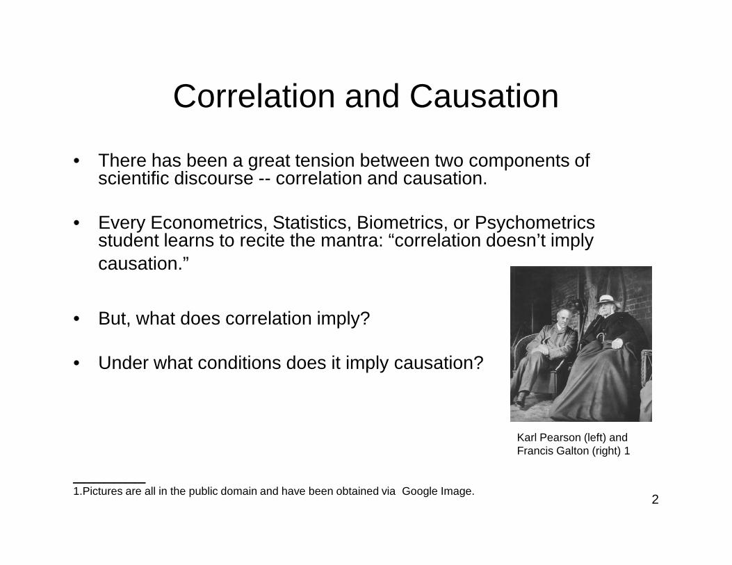
• There has been a great tension between two components of scientific discourse -- correlation and causation.

• Every Econometrics, Statistics, Biometrics, or Psychometrics student learns to recite the mantra: “correlation doesn’t imply causation.”

2

• But, what does correlation imply?

• Under what conditions does it imply causation?

_______1.Pictures are all in the public domain and have been obtained via Google Image.

Karl Pearson (left) and Francis Galton (right) 1

Correlation: A Measure of Linear Association Between X and Y

The population correlation coefficient ρ(X,Y) between two random variables X and Y with expected values of µX and µY and standard deviations σX and σY is given as:

ρ(X,Y) = E{(X- µX)(Y- µY)}/ σXσY

where E is the expectation operator.

3

It is the case that -1≤ ρ ≤ +1. This theoretical representation is replaced with frequency calculations from data on X and Y in empirical settings.

This measure was invented by Galton in the 19th century and used extensively by Pearson in the early 20th century (previous slide)1._________1. See Galton, F. (1888) “Co-relations and their measurement, chiefly from anthropological data,” Proceedings of the Royal Society of London 45:135-45. See as well, Pearson, K. (1920) “Notes on the History of Correlation,” Biometrika 12:25-45.

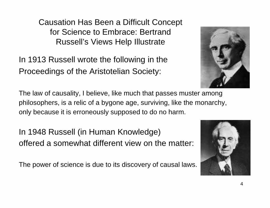
Causation Has Been a Difficult Concept for Science to Embrace: Bertrand

Russell’s Views Help Illustrate

In 1913 Russell wrote the following in the Proceedings of the Aristotelian Society:

The law of causality, I believe, like much that passes muster amongphilosophers, is a relic of a bygone age, surviving, like the monarchy,

4

philosophers, is a relic of a bygone age, surviving, like the monarchy,only because it is erroneously supposed to do no harm.

In 1948 Russell (in Human Knowledge)offered a somewhat different view on the matter:

The power of science is due to its discovery of causal laws.

Causation

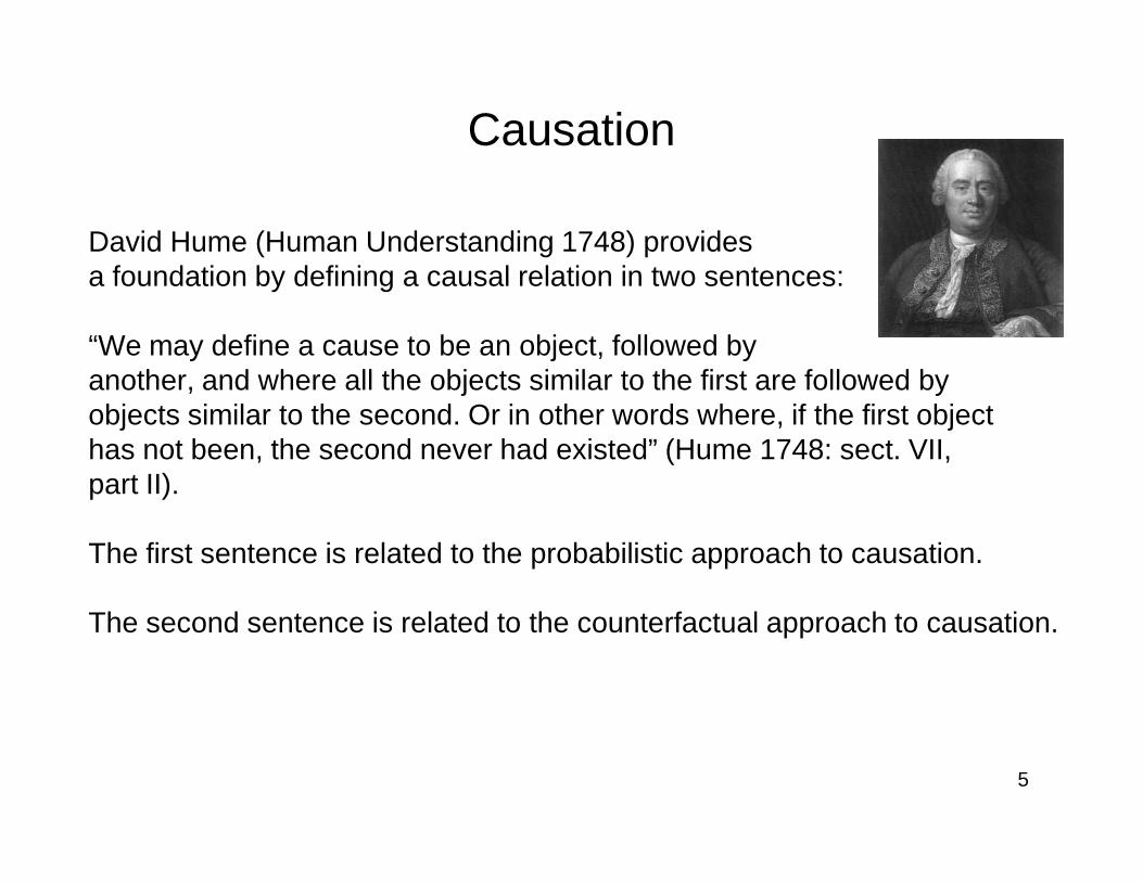
David Hume (Human Understanding 1748) provides a foundation by defining a causal relation in two sentences:

“We may define a cause to be an object, followed by another, and where all the objects similar to the first are followed by objects similar to the second. Or in other words where, if the first object has not been, the second never had existed” (Hume 1748: sect. VII,

5

has not been, the second never had existed” (Hume 1748: sect. VII, part II).

The first sentence is related to the probabilistic approach to causation.

The second sentence is related to the counterfactual approach to causation.

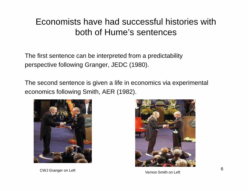
Economists have had successful histories with both of Hume’s sentences

The first sentence can be interpreted from a predictabilityperspective following Granger, JEDC (1980).

The second sentence is given a life in economics via experimentaleconomics following Smith, AER (1982).

6CWJ Granger on Left Vernon Smith on Left

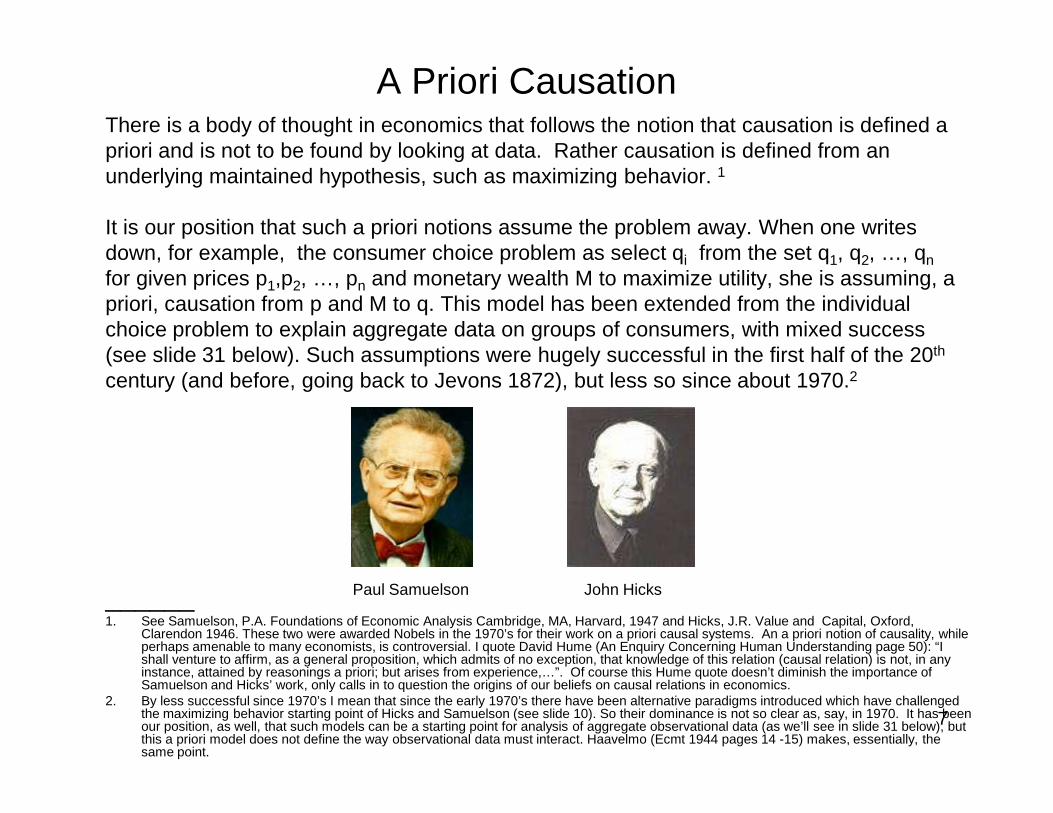
A Priori CausationThere is a body of thought in economics that follows the notion that causation is defined a priori and is not to be found by looking at data. Rather causation is defined from an underlying maintained hypothesis, such as maximizing behavior. 1

It is our position that such a priori notions assume the problem away. When one writes down, for example, the consumer choice problem as select qi from the set q1, q2, …, qnfor given prices p1,p2, …, pn and monetary wealth M to maximize utility, she is assuming, a priori, causation from p and M to q. This model has been extended from the individual choice problem to explain aggregate data on groups of consumers, with mixed success (see slide 31 below). Such assumptions were hugely successful in the first half of the 20th

century (and before, going back to Jevons 1872), but less so since about 1970.2

7

______1. See Samuelson, P.A. Foundations of Economic Analysis Cambridge, MA, Harvard, 1947 and Hicks, J.R. Value and Capital, Oxford,

Clarendon 1946. These two were awarded Nobels in the 1970’s for their work on a priori causal systems. An a priori notion of causality, while perhaps amenable to many economists, is controversial. I quote David Hume (An Enquiry Concerning Human Understanding page 50): “I shall venture to affirm, as a general proposition, which admits of no exception, that knowledge of this relation (causal relation) is not, in any instance, attained by reasonings a priori; but arises from experience,…”. Of course this Hume quote doesn’t diminish the importance of Samuelson and Hicks’ work, only calls in to question the origins of our beliefs on causal relations in economics.

2. By less successful since 1970’s I mean that since the early 1970’s there have been alternative paradigms introduced which have challenged the maximizing behavior starting point of Hicks and Samuelson (see slide 10). So their dominance is not so clear as, say, in 1970. It has been our position, as well, that such models can be a starting point for analysis of aggregate observational data (as we’ll see in slide 31 below), but this a priori model does not define the way observational data must interact. Haavelmo (Ecmt 1944 pages 14 -15) makes, essentially, the same point.

Paul Samuelson John Hicks

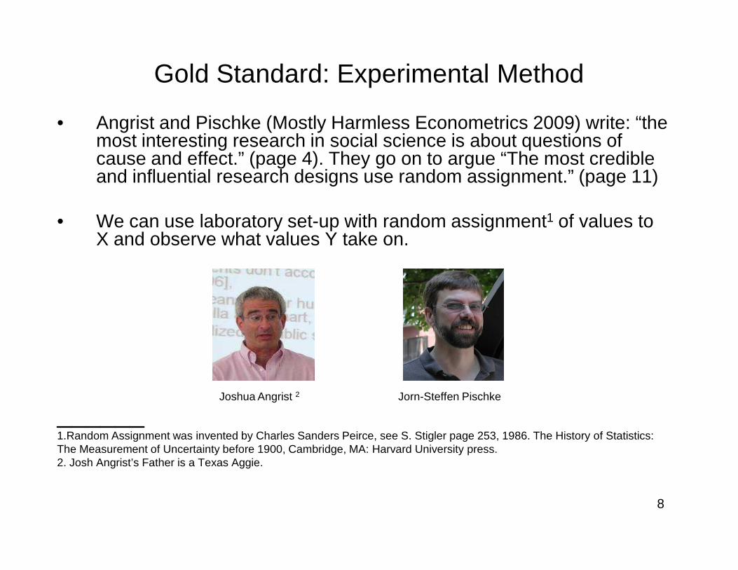
Gold Standard: Experimental Method

• Angrist and Pischke (Mostly Harmless Econometrics 2009) write: “the most interesting research in social science is about questions of cause and effect.” (page 4). They go on to argue “The most credible and influential research designs use random assignment.” (page 11)

• We can use laboratory set-up with random assignment1 of values to X and observe what values Y take on.

8

______1.Random Assignment was invented by Charles Sanders Peirce, see S. Stigler page 253, 1986. The History of Statistics: The Measurement of Uncertainty before 1900, Cambridge, MA: Harvard University press.2. Josh Angrist’s Father is a Texas Aggie.

Joshua Angrist 2 Jorn-Steffen Pischke

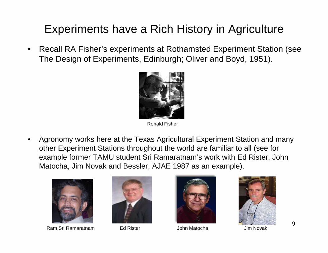
Experiments have a Rich History in Agriculture

• Recall RA Fisher’s experiments at Rothamsted Experiment Station (see The Design of Experiments, Edinburgh; Oliver and Boyd, 1951).

Ronald Fisher

9

• Agronomy works here at the Texas Agricultural Experiment Station and many other Experiment Stations throughout the world are familiar to all (see for example former TAMU student Sri Ramaratnam’s work with Ed Rister, John Matocha, Jim Novak and Bessler, AJAE 1987 as an example).

Ed Rister John MatochaRam Sri Ramaratnam Jim Novak

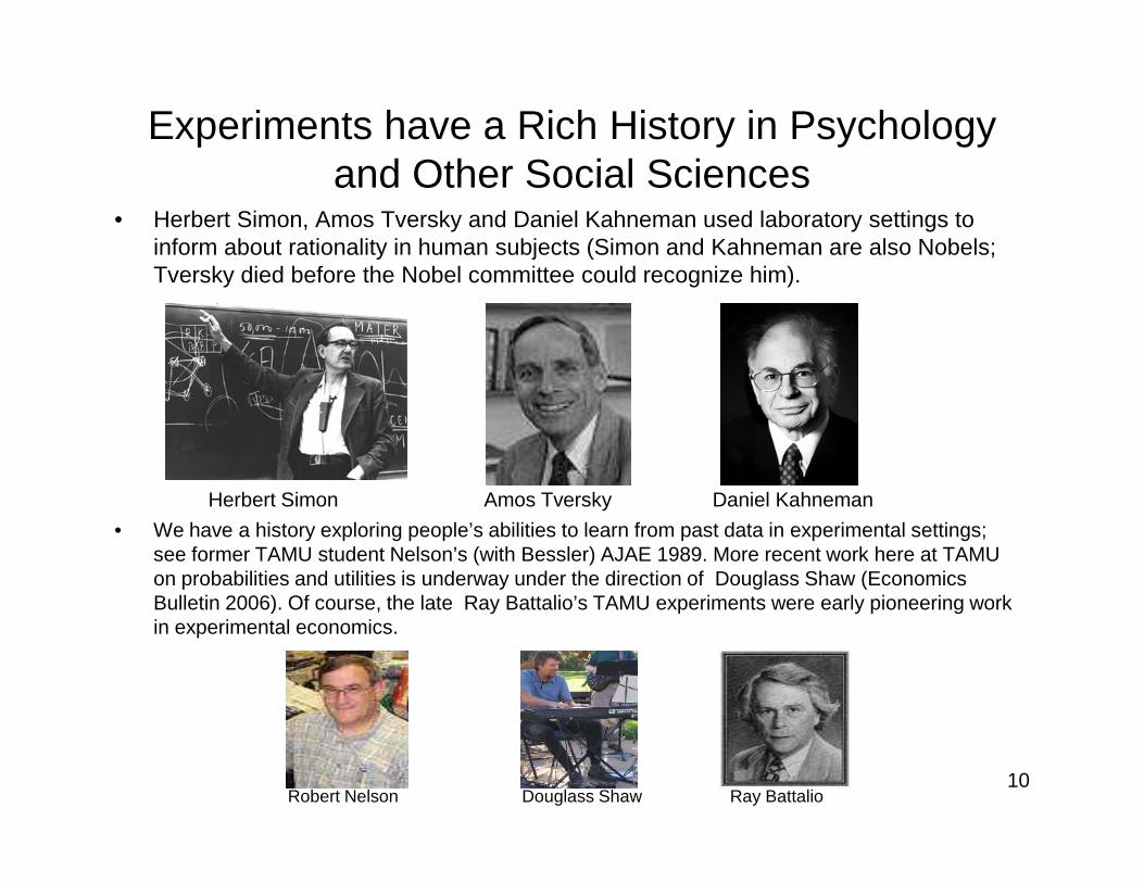
Experiments have a Rich History in Psychology and Other Social Sciences

• Herbert Simon, Amos Tversky and Daniel Kahneman used laboratory settings to inform about rationality in human subjects (Simon and Kahneman are also Nobels; Tversky died before the Nobel committee could recognize him).

10

Herbert Simon Amos Tversky Daniel Kahneman

• We have a history exploring people’s abilities to learn from past data in experimental settings; see former TAMU student Nelson’s (with Bessler) AJAE 1989. More recent work here at TAMU on probabilities and utilities is underway under the direction of Douglass Shaw (Economics Bulletin 2006). Of course, the late Ray Battalio’s TAMU experiments were early pioneering work in experimental economics.

Robert Nelson Douglass Shaw Ray Battalio

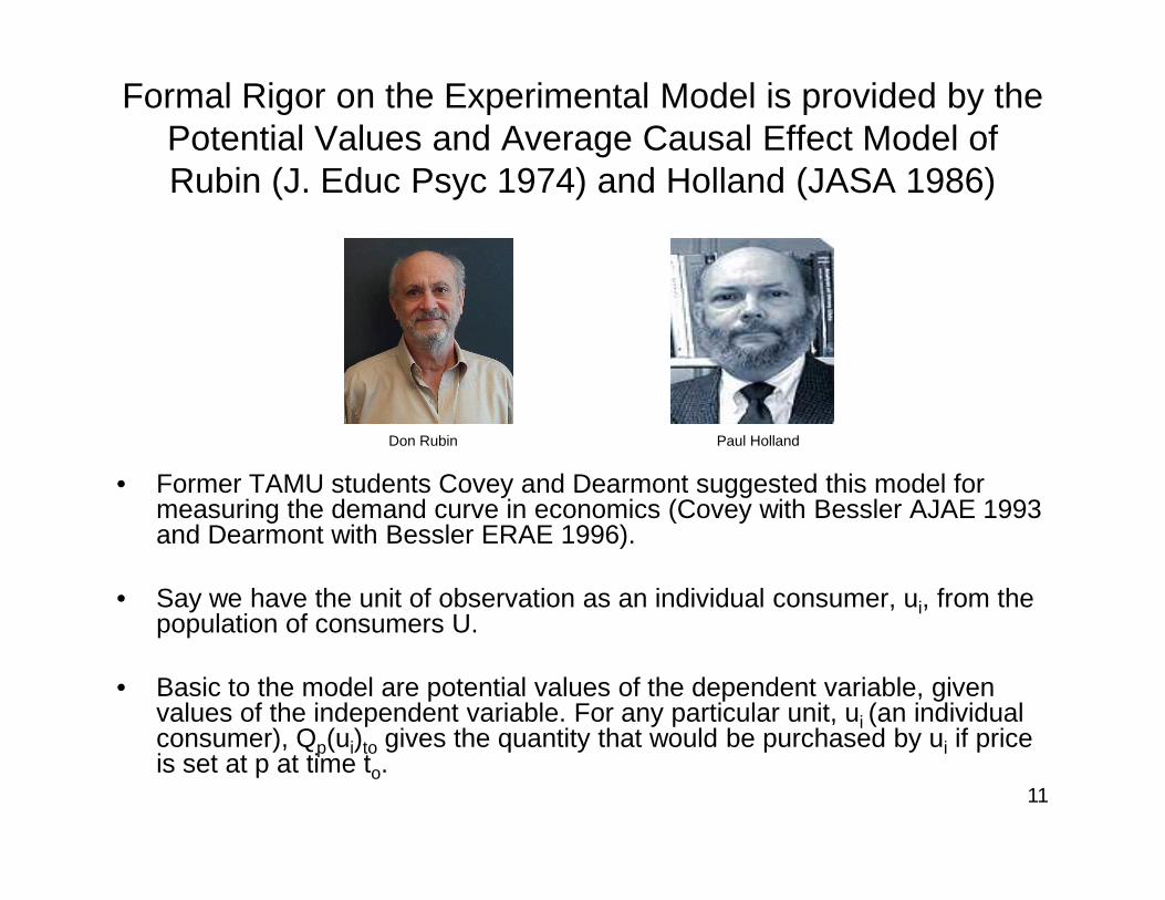
Formal Rigor on the Experimental Model is provided by the Potential Values and Average Causal Effect Model of Rubin (J. Educ Psyc 1974) and Holland (JASA 1986)

Don Rubin Paul Holland

11

• Former TAMU students Covey and Dearmont suggested this model for measuring the demand curve in economics (Covey with Bessler AJAE 1993 and Dearmont with Bessler ERAE 1996).

• Say we have the unit of observation as an individual consumer, ui, from the population of consumers U.

• Basic to the model are potential values of the dependent variable, given values of the independent variable. For any particular unit, ui (an individual consumer), Qp(ui)to gives the quantity that would be purchased by ui if price is set at p at time to.

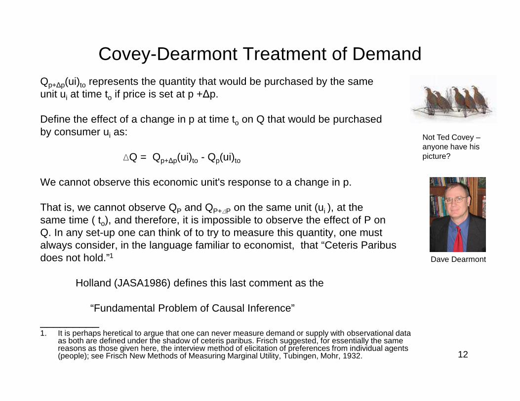
Covey-Dearmont Treatment of DemandQp+∆p(ui)to represents the quantity that would be purchased by the same unit ui at time to if price is set at p +∆p.

Define the effect of a change in p at time to on Q that would be purchased by consumer ui as:

)Q = Qp+∆p(ui)to - Qp(ui)to

We cannot observe this economic unit's response to a change in p.

Not Ted Covey –anyone have his picture?

12

That is, we cannot observe QP and QP+)P on the same unit (ui ), at the same time ( to), and therefore, it is impossible to observe the effect of P on Q. In any set-up one can think of to try to measure this quantity, one must always consider, in the language familiar to economist, that “Ceteris Paribus does not hold.”1

Holland (JASA1986) defines this last comment as the

“Fundamental Problem of Causal Inference”_________1. It is perhaps heretical to argue that one can never measure demand or supply with observational data

as both are defined under the shadow of ceteris paribus. Frisch suggested, for essentially the same reasons as those given here, the interview method of elicitation of preferences from individual agents (people); see Frisch New Methods of Measuring Marginal Utility, Tubingen, Mohr, 1932.

Dave Dearmont

But,

if we observe several units (ui’s) and assign them randomly to control p or treatment p+∆p, then we can observed the “average causal effect ” of p+∆prelative to p on a set of subjects.

So for Holland (JASA 1986) causation is relative, that is the causal effect of the treatment (p+∆p) is relative to the control (p).

My reading of Holland puts us squarely in the laboratory in our study of causation.

13

Yet his colleague, Don Rubin (1974, page 688), appears more open to study in non-laboratory settings:

“…to ignore existing observational data may be counter-productive. It seems more reasonable to try to estimate the effects of the treatments from nonrandomized studies than to ignore these data and dream of the ideal experiment or make “armchair” decisions without the benefit of data analysis.”1

______________1.Rubin goes on to propose the study causal effects in observational data by introducing propensity score matching. We don’t follow this step, as understanding the causal structure of the confounding variables is a non-trivial problem that propensity score matching seems not to have addressed; see Pearl 2009 for discussion.

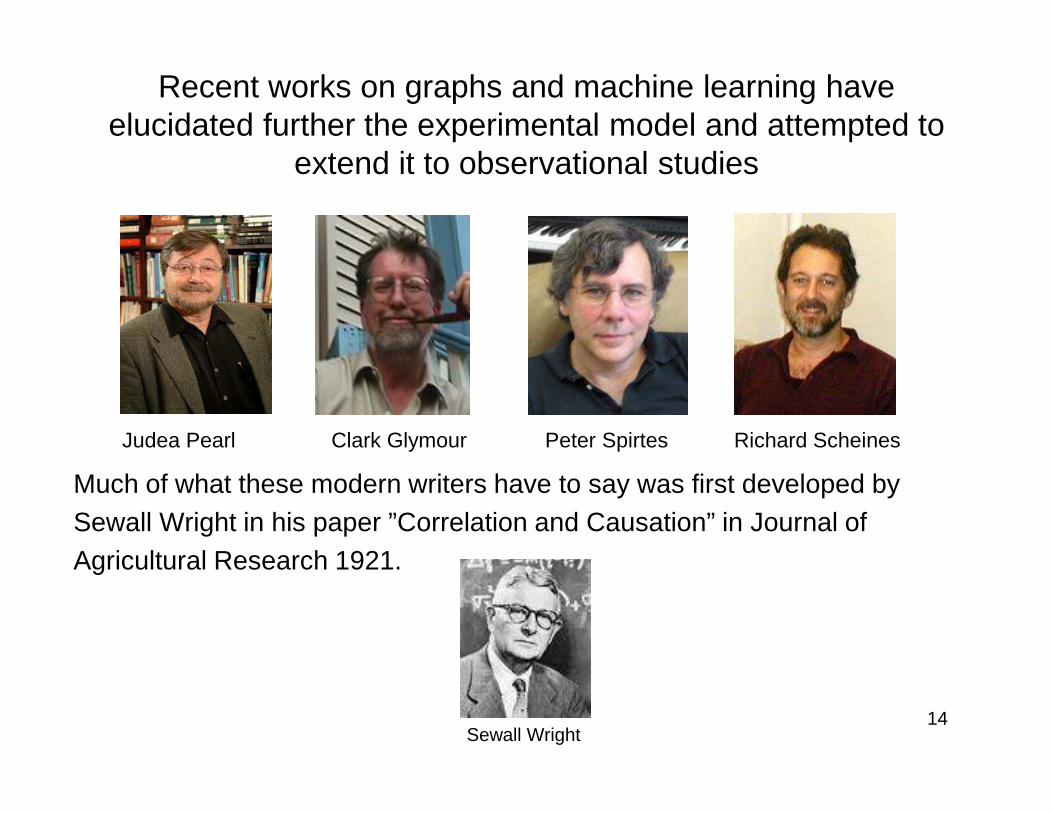
Recent works on graphs and machine learning have elucidated further the experimental model and attempted to

extend it to observational studies

14

Judea Pearl Clark Glymour Peter Spirtes Richard Scheines

Much of what these modern writers have to say was first developed by Sewall Wright in his paper ”Correlation and Causation” in Journal of Agricultural Research 1921.

Sewall Wright

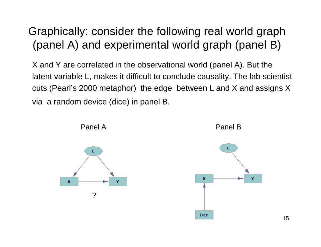
Graphically: consider the following real world graph (panel A) and experimental world graph (panel B)

X and Y are correlated in the observational world (panel A). But the latent variable L, makes it difficult to conclude causality. The lab scientist cuts (Pearl’s 2000 metaphor) the edge between L and X and assigns X

via a random device (dice) in panel B.

Panel A Panel B

15

Panel A Panel B

??

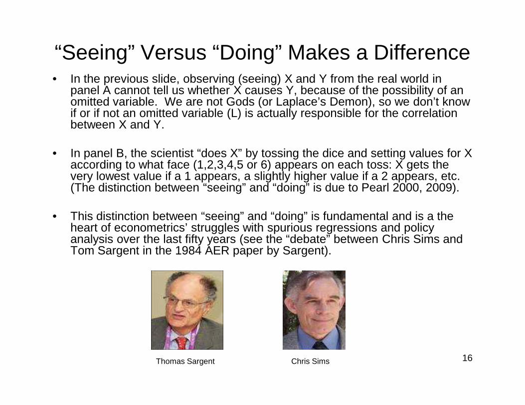
“Seeing” Versus “Doing” Makes a Difference• In the previous slide, observing (seeing) X and Y from the real world in

panel A cannot tell us whether X causes Y, because of the possibility of an omitted variable. We are not Gods (or Laplace’s Demon), so we don’t know if or if not an omitted variable (L) is actually responsible for the correlation between X and Y.

• In panel B, the scientist “does X” by tossing the dice and setting values for X according to what face (1,2,3,4,5 or 6) appears on each toss: X gets the very lowest value if a 1 appears, a slightly higher value if a 2 appears, etc. (The distinction between “seeing” and “doing” is due to Pearl 2000, 2009).

16

• This distinction between “seeing” and “doing” is fundamental and is a the heart of econometrics’ struggles with spurious regressions and policy analysis over the last fifty years (see the “debate” between Chris Sims and Tom Sargent in the 1984 AER paper by Sargent).

Thomas Sargent Chris Sims

Going to the observational world requires more assumptions because we can’t toss the dice to

answer many questions

• For a data set (x1, X2 , x3, …, Xn ) , we can find its generating causal structure (identify such structure) if we have the following conditions:

• Causal Sufficiency: There are no omitted variables that cause two or more of the included variables.

17

or more of the included variables.

• Markov Condition: We can write probabilities of variables by conditioning just on each variable’s parents.

• Faithfulness Condition: If we see zero correlation between two variables, the reason we see it is because there is no edge between these variables and not cancellation of structural parameters.

Algorithms of Inductive Causation

The three conditions on the previous slide have been thebasis for a rich literature in inductive causation.

This work has been centered at Carnegie Mellon University (Spirtes, Glymour and Scheines) and UCLA (Pearl); see slide 14.

18

(Pearl); see slide 14.

Below we explore the three conditions which allow us to conclude some correlations found in observational data do represent causal structures, while others do not. We discuss these under the label “Algorithms of Inductive Causation.”

Causal Sufficiency

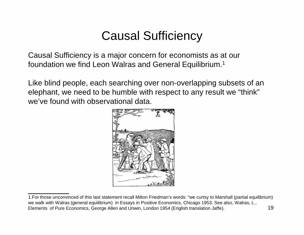
Causal Sufficiency is a major concern for economists as at our foundation we find Leon Walras and General Equilibrium.1

Like blind people, each searching over non-overlapping subsets of an elephant, we need to be humble with respect to any result we “think” we’ve found with observational data.

19

________1.For those unconvinced of this last statement recall Milton Friedman’s words: “we curtsy to Marshall (partial equilibrium) we walk with Walras (general equilibrium) in Essays in Positive Economics, Chicago 1953. See also, Walras, L., Elements of Pure Economics, George Allen and Unwin, London 1954 (English translation Jaffe).

More on Causal Sufficiency

• In the blind persons’ search (previous slide) over subsets of the elephant, one person may think she’s found a snake (trunk), another a brush (tail), yet another a plough (tusk).

• The Buddha speaks of such search in the following verse:

20

O how they cling and wrangle, some who claim For preacher and monk the honored name! For, quarreling, each to his view they cling. Such folk see only one side of a thing.

_________Quote and elephant picture from Wikipedia

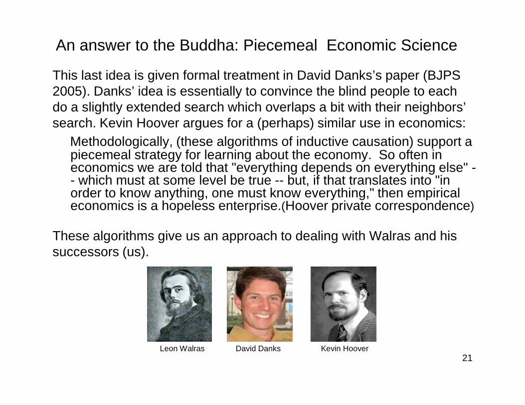
An answer to the Buddha: Piecemeal Economic Science

This last idea is given formal treatment in David Danks’s paper (BJPS 2005). Danks’ idea is essentially to convince the blind people to each do a slightly extended search which overlaps a bit with their neighbors’search. Kevin Hoover argues for a (perhaps) similar use in economics:

Methodologically, (these algorithms of inductive causation) support a piecemeal strategy for learning about the economy. So often in economics we are told that "everything depends on everything else" -- which must at some level be true -- but, if that translates into "in order to know anything, one must know everything," then empirical economics is a hopeless enterprise.(Hoover private correspondence)

21

economics is a hopeless enterprise.(Hoover private correspondence)

These algorithms give us an approach to dealing with Walras and his successors (us).

Leon Walras David Danks Kevin Hoover

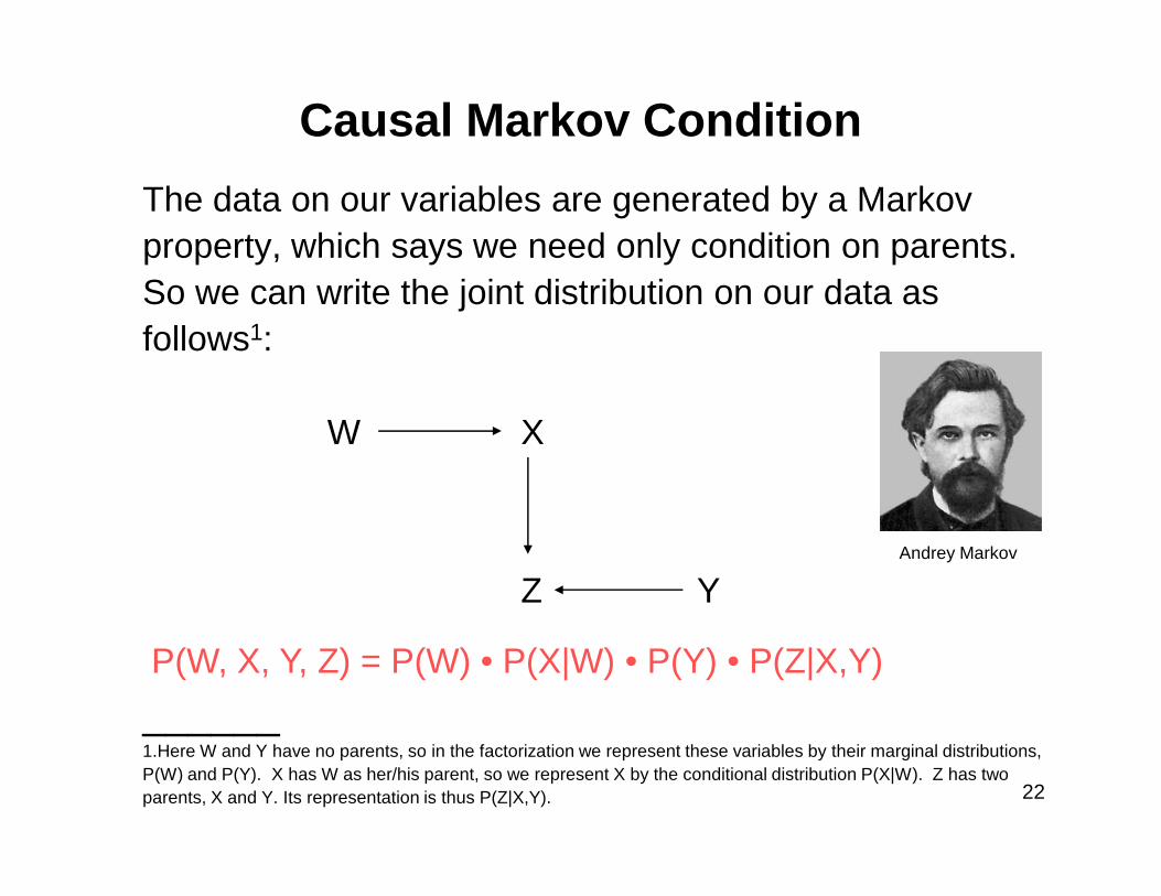
Causal Markov Condition

The data on our variables are generated by a Markov property, which says we need only condition on parents. So we can write the joint distribution on our data as follows1:

XW

22

______1.Here W and Y have no parents, so in the factorization we represent these variables by their marginal distributions, P(W) and P(Y). X has W as her/his parent, so we represent X by the conditional distribution P(X|W). Z has two parents, X and Y. Its representation is thus P(Z|X,Y).

Z

X

Y

W

P(W, X, Y, Z) = P(W) • P(X|W) • P(Y) • P(Z|X,Y)

Andrey Markov

Faithfulness

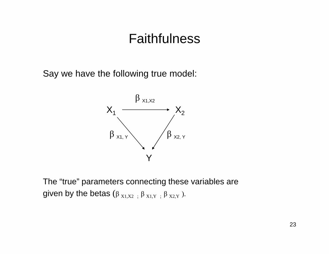
Say we have the following true model:

β X1,X2

X1 X2

23

β X1, Y β X2, Y

Y

The “true” parameters connecting these variables are given by the betas (β X1,X2 ; β X1,Y ; β X2,Y ).

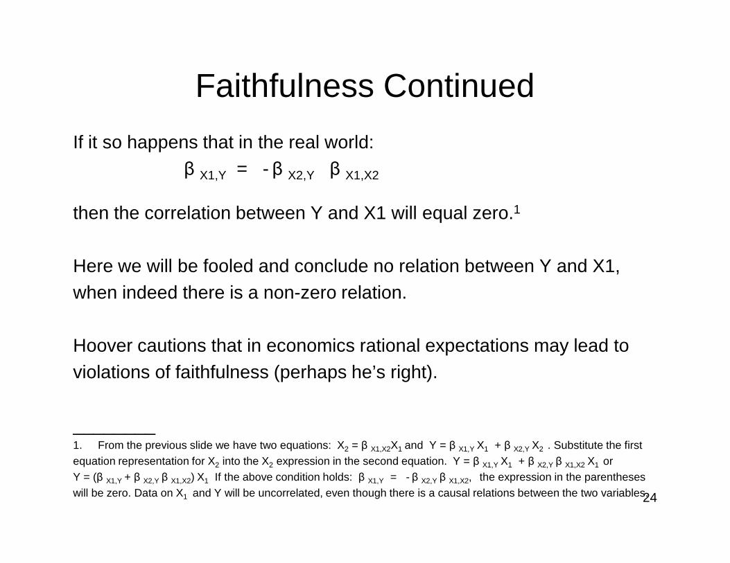
Faithfulness Continued

If it so happens that in the real world: β X1,Y = - β X2,Y β X1,X2

then the correlation between Y and X1 will equal zero.1

Here we will be fooled and conclude no relation between Y and X1,

24

when indeed there is a non-zero relation.

Hoover cautions that in economics rational expectations may lead to violations of faithfulness (perhaps he’s right).

________1. From the previous slide we have two equations: X2 = β X1,X2X1 and Y = β X1,Y X1 + β X2,Y X2 . Substitute the first equation representation for X2 into the X2 expression in the second equation. Y = β X1,Y X1 + β X2,Y β X1,X2 X1 orY = (β X1,Y + β X2,Y β X1,X2) X1 If the above condition holds: β X1,Y = - β X2,Y β X1,X2, the expression in the parentheses will be zero. Data on X1 and Y will be uncorrelated, even though there is a causal relations between the two variables.

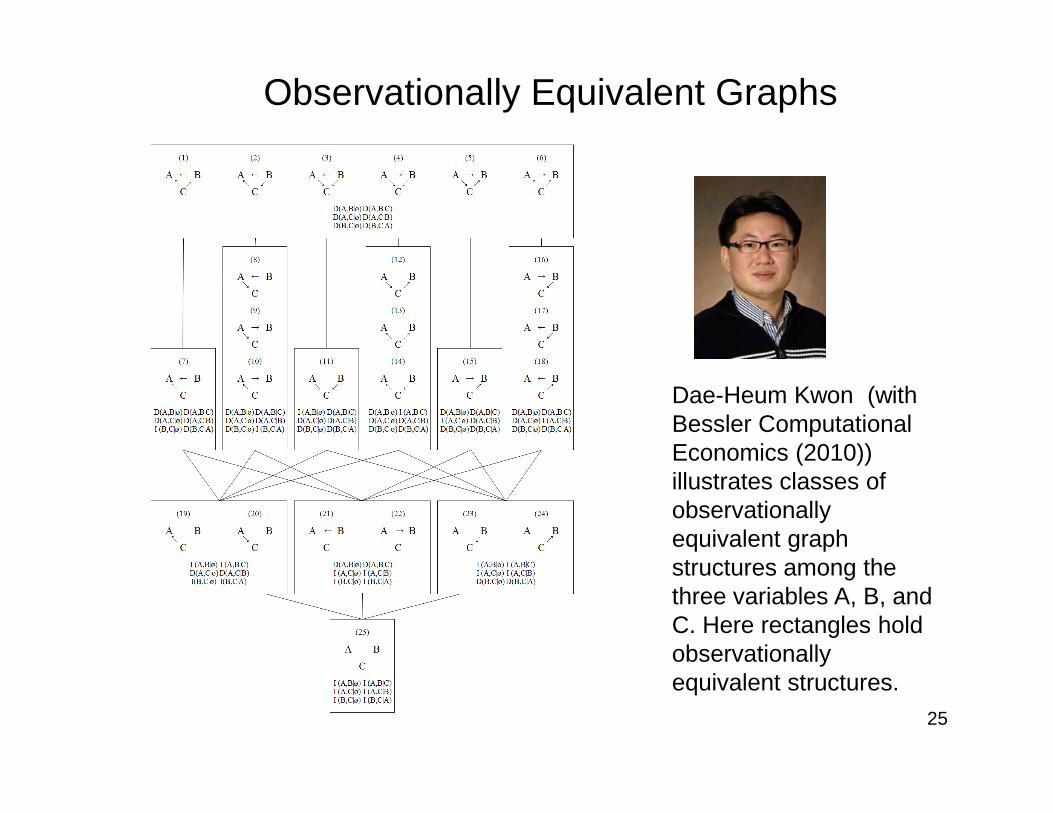
Observationally Equivalent Graphs

Dae-Heum Kwon (with

25

Dae-Heum Kwon (with Bessler Computational Economics (2010)) illustrates classes of observationally equivalent graph structures among the three variables A, B, and C. Here rectangles hold observationally equivalent structures.

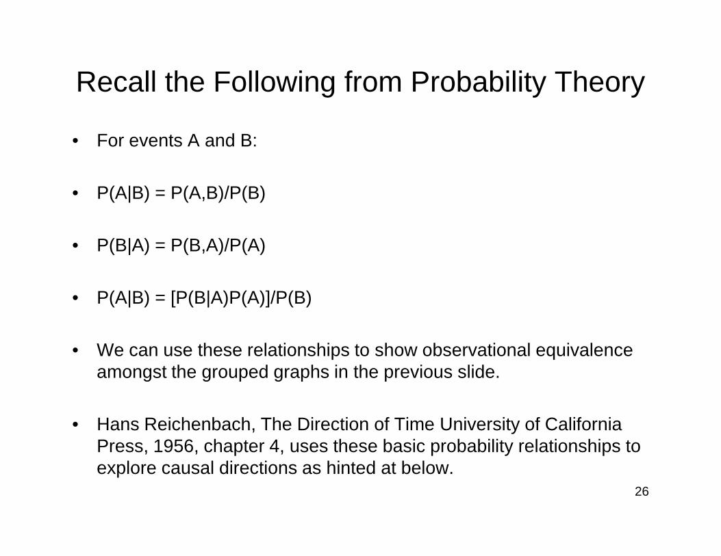
Recall the Following from Probability Theory

• For events A and B:

• P(A|B) = P(A,B)/P(B)

• P(B|A) = P(B,A)/P(A)

26

• P(A|B) = [P(B|A)P(A)]/P(B)

• We can use these relationships to show observational equivalence amongst the grouped graphs in the previous slide.

• Hans Reichenbach, The Direction of Time University of California Press, 1956, chapter 4, uses these basic probability relationships to explore causal directions as hinted at below.

Consider Graphs (19) and (20) from Slide 251

Panel A Graph (19) Panel B Graph (20)

P(A,B,C) = P(C)P(B)P(A|C) P(A,B,C) = P(A)P(B)P(C|A)= {P(C)P(B)[P(C|A)P(A)]}/P(C) = {P(A)P(B)[P(A|C)P(C)]}/P(A) = P(A)P(B)P(C|A) = P(C)P(B)P(A|C)

27

= P(A)P(B)P(C|A) = P(C)P(B)P(A|C)

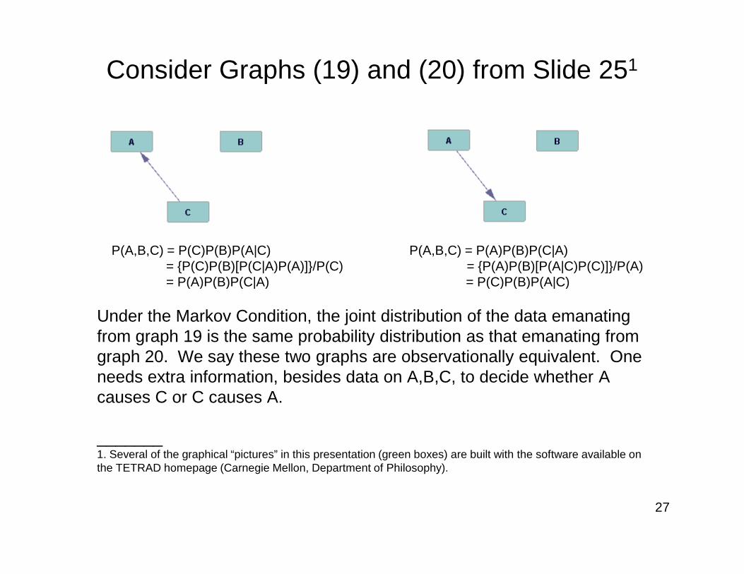
Under the Markov Condition, the joint distribution of the data emanating from graph 19 is the same probability distribution as that emanating from graph 20. We say these two graphs are observationally equivalent. One needs extra information, besides data on A,B,C, to decide whether A causes C or C causes A.

_______1. Several of the graphical “pictures” in this presentation (green boxes) are built with the software available on the TETRAD homepage (Carnegie Mellon, Department of Philosophy).

Consider Graphs (16) and (18) from slide 25

Panel A (16) Panel B (18)

• P(A,B,C) = P(A)P(B|A)P(C|B) P(A,B,C)= P(C)P(B|C)P(A|B)• = {P(A)P(A|B) P(B)P(C|B)}/P(A) = {P(C)P(C|B)P(B)P(A|B)}/P(C)

28

• = {P(A)P(A|B) P(B)P(C|B)}/P(A) = {P(C)P(C|B)P(B)P(A|B)}/P(C)• = P(B)P(A|B)P(C|B) =P(B)P(A|B)P(C|B)• ={P(B)P(A|B)P(B|C)P(C)}/P(B) ={P(B)P(B|A)P(A)P(C|B)}/P(B)• =P(A|B)P(B|C)P(C) =P(A)P(B|A)P(C|B)

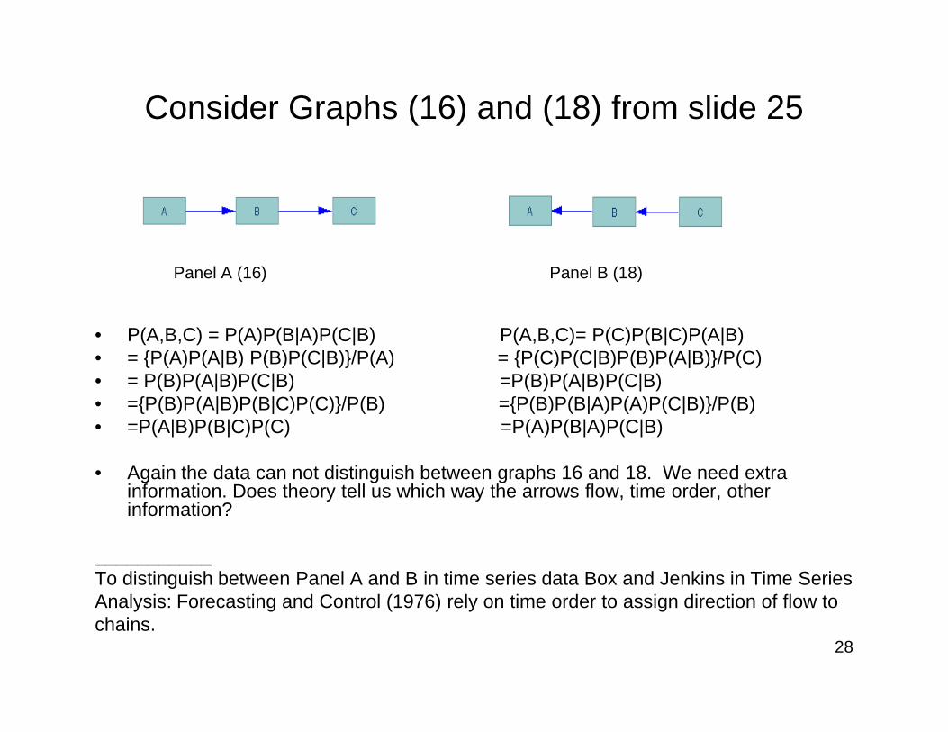
• Again the data can not distinguish between graphs 16 and 18. We need extra information. Does theory tell us which way the arrows flow, time order, other information?

___________To distinguish between Panel A and B in time series data Box and Jenkins in Time Series Analysis: Forecasting and Control (1976) rely on time order to assign direction of flow to chains.

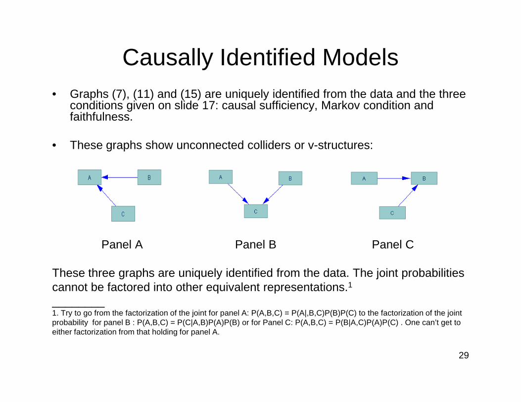
Causally Identified Models• Graphs (7), (11) and (15) are uniquely identified from the data and the three

conditions given on slide 17: causal sufficiency, Markov condition and faithfulness.

• These graphs show unconnected colliders or v-structures:

29

Panel A Panel B Panel C

These three graphs are uniquely identified from the data. The joint probabilities cannot be factored into other equivalent representations.1

________1. Try to go from the factorization of the joint for panel A: P(A,B,C) = P(A|,B,C)P(B)P(C) to the factorization of the joint probability for panel B : P(A,B,C) = P(C|A,B)P(A)P(B) or for Panel C: P(A,B,C) = P(B|A,C)P(A)P(C) . One can’t get to either factorization from that holding for panel A.

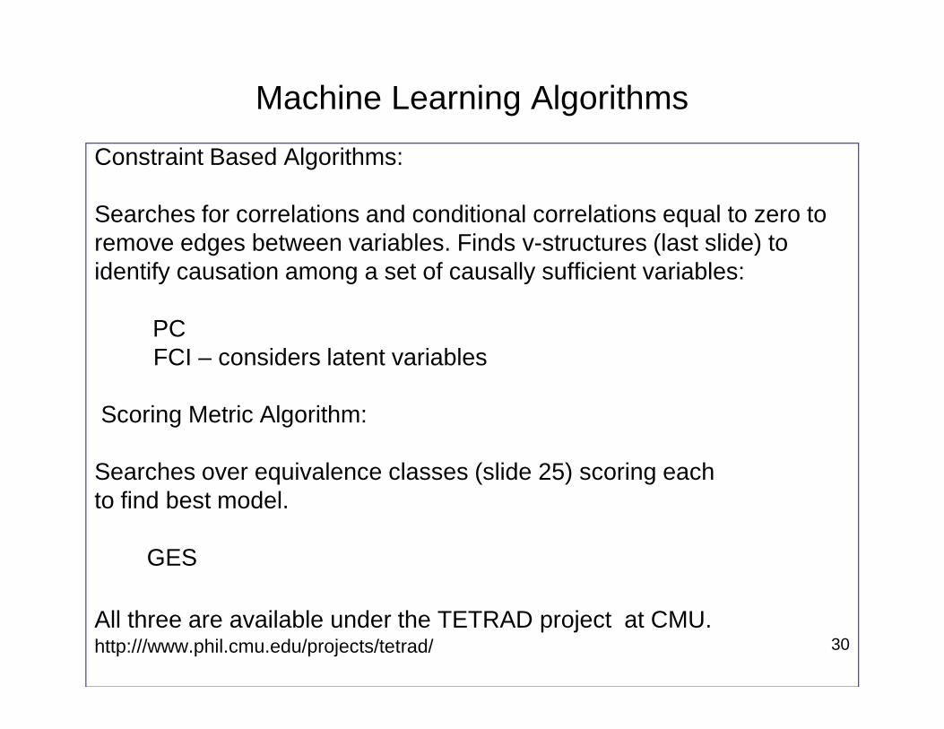
Machine Learning Algorithms

Constraint Based Algorithms:

Searches for correlations and conditional correlations equal to zero to remove edges between variables. Finds v-structures (last slide) to identify causation among a set of causally sufficient variables:

PCFCI – considers latent variables

30

FCI – considers latent variables

Scoring Metric Algorithm:

Searches over equivalence classes (slide 25) scoring each to find best model.

GES

All three are available under the TETRAD project at CMU. http:///www.phil.cmu.edu/projects/tetrad/

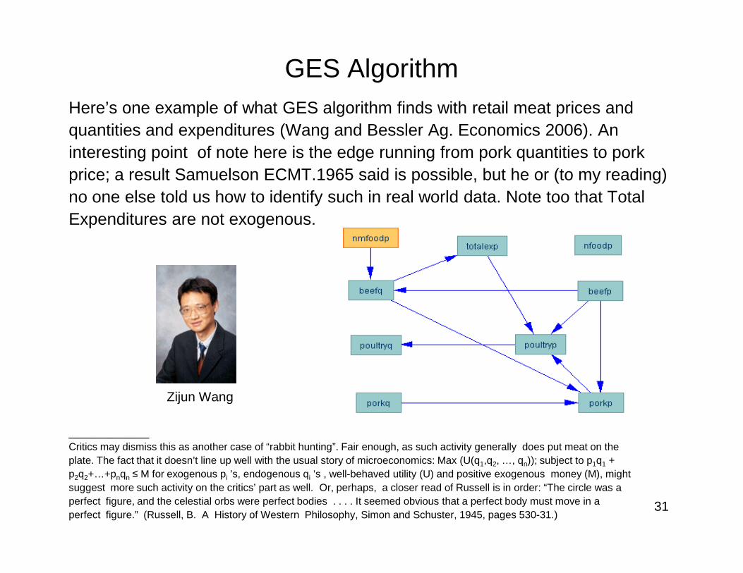
GES AlgorithmHere’s one example of what GES algorithm finds with retail meat prices and quantities and expenditures (Wang and Bessler Ag. Economics 2006). An interesting point of note here is the edge running from pork quantities to pork price; a result Samuelson ECMT.1965 said is possible, but he or (to my reading) no one else told us how to identify such in real world data. Note too that Total Expenditures are not exogenous.

31

Zijun Wang

___________Critics may dismiss this as another case of “rabbit hunting”. Fair enough, as such activity generally does put meat on the plate. The fact that it doesn’t line up well with the usual story of microeconomics: Max (U(q1,q2, …, qn)); subject to p1q1 + p2q2+…+pnqn ≤ M for exogenous pi ’s, endogenous qi ’s , well-behaved utility (U) and positive exogenous money (M), might suggest more such activity on the critics’ part as well. Or, perhaps, a closer read of Russell is in order: “The circle was aperfect figure, and the celestial orbs were perfect bodies . . . . It seemed obvious that a perfect body must move in a perfect figure.” (Russell, B. A History of Western Philosophy, Simon and Schuster, 1945, pages 530-31.)

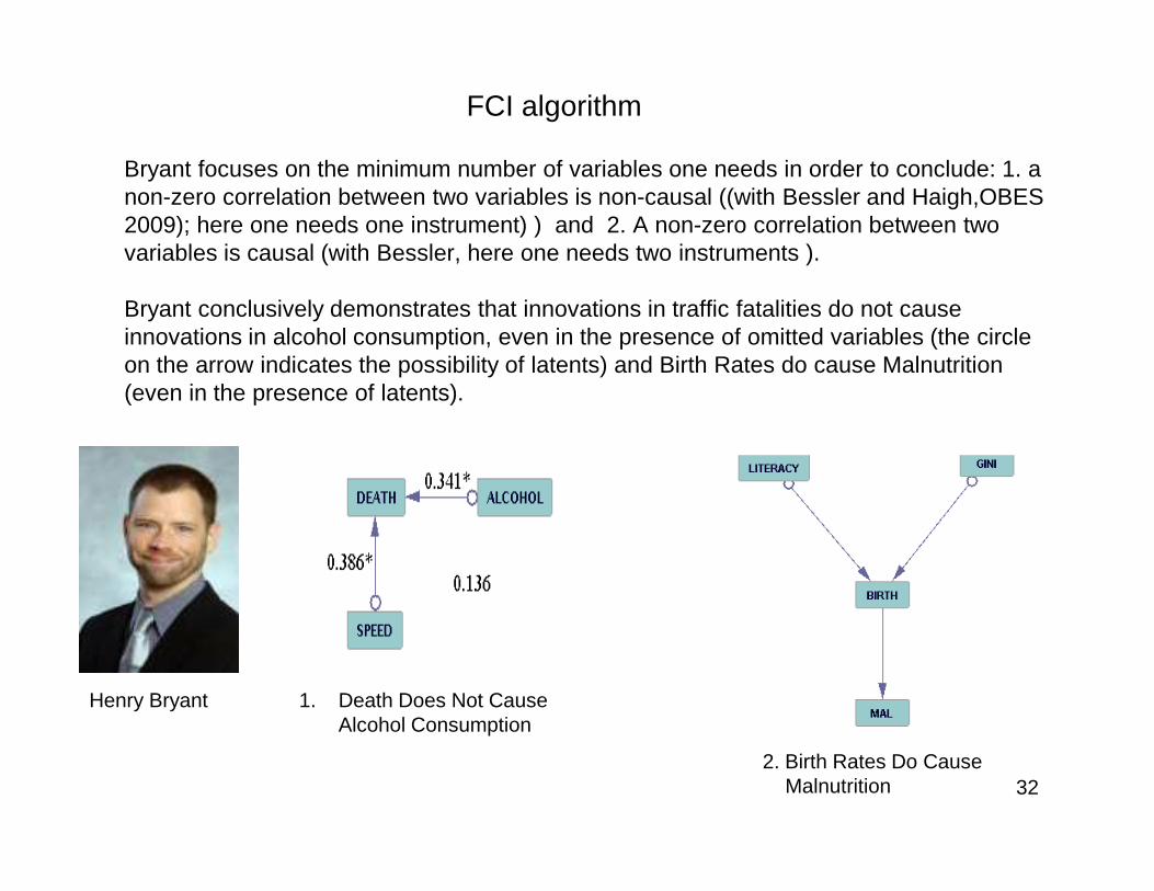
FCI algorithm

Bryant focuses on the minimum number of variables one needs in order to conclude: 1. a non-zero correlation between two variables is non-causal ((with Bessler and Haigh,OBES2009); here one needs one instrument) ) and 2. A non-zero correlation between two variables is causal (with Bessler, here one needs two instruments ).

Bryant conclusively demonstrates that innovations in traffic fatalities do not cause innovations in alcohol consumption, even in the presence of omitted variables (the circle on the arrow indicates the possibility of latents) and Birth Rates do cause Malnutrition (even in the presence of latents).

32

Henry Bryant 1. Death Does Not Cause Alcohol Consumption

2. Birth Rates Do Cause Malnutrition

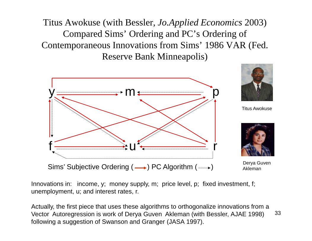
Titus Awokuse (with Bessler, Jo.Applied Economics 2003) Compared Sims’ Ordering and PC’s Ordering of

Contemporaneous Innovations from Sims’ 1986 VAR (Fed. Reserve Bank Minneapolis)

y m pTitus Awokuse

33

f u r

Sims’ Subjective Ordering ( ) PC Algorithm ( )

Innovations in: income, y; money supply, m; price level, p; fixed investment, f; unemployment, u; and interest rates, r.

Actually, the first piece that uses these algorithms to orthogonalize innovations from a Vector Autoregression is work of Derya Guven Akleman (with Bessler, AJAE 1998) following a suggestion of Swanson and Granger (JASA 1997).

Derya Guven Akleman

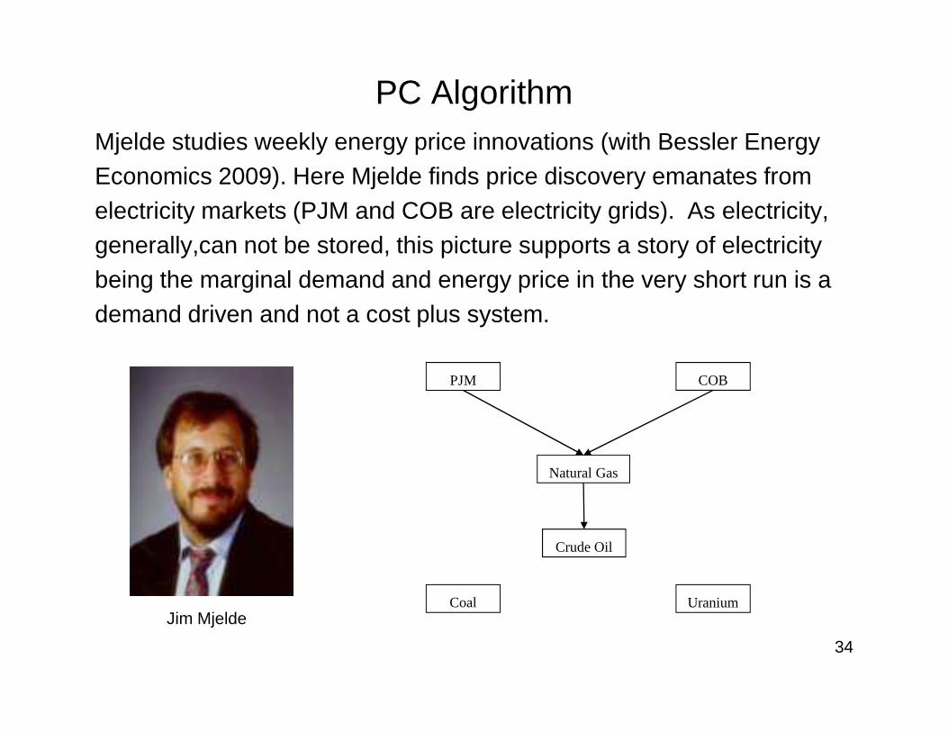
PC AlgorithmMjelde studies weekly energy price innovations (with Bessler Energy Economics 2009). Here Mjelde finds price discovery emanates from electricity markets (PJM and COB are electricity grids). As electricity, generally,can not be stored, this picture supports a story of electricity being the marginal demand and energy price in the very short run is a demand driven and not a cost plus system.

34

PJM COB

Natural Gas

Coal Uranium

Crude Oil

Jim Mjelde

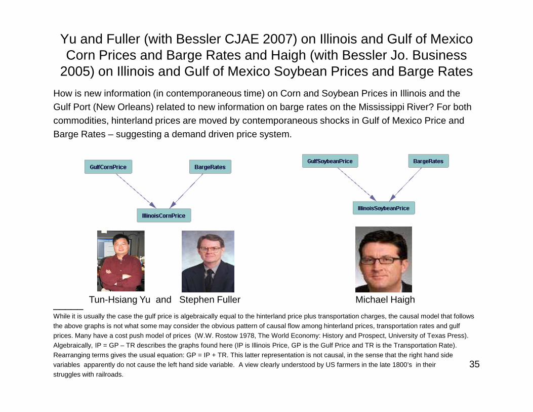
Yu and Fuller (with Bessler CJAE 2007) on Illinois and Gulf of Mexico Corn Prices and Barge Rates and Haigh (with Bessler Jo. Business

2005) on Illinois and Gulf of Mexico Soybean Prices and Barge Rates

How is new information (in contemporaneous time) on Corn and Soybean Prices in Illinois and the Gulf Port (New Orleans) related to new information on barge rates on the Mississippi River? For both commodities, hinterland prices are moved by contemporaneous shocks in Gulf of Mexico Price and Barge Rates – suggesting a demand driven price system.

35

_____ While it is usually the case the gulf price is algebraically equal to the hinterland price plus transportation charges, the causal model that follows

the above graphs is not what some may consider the obvious pattern of causal flow among hinterland prices, transportation rates and gulf

prices. Many have a cost push model of prices (W.W. Rostow 1978, The World Economy: History and Prospect, University of Texas Press).

Algebraically, IP = GP – TR describes the graphs found here (IP is Illinois Price, GP is the Gulf Price and TR is the Transportation Rate).

Rearranging terms gives the usual equation: GP = IP + TR. This latter representation is not causal, in the sense that the right hand side

variables apparently do not cause the left hand side variable. A view clearly understood by US farmers in the late 1800’s in their

struggles with railroads.

Michael HaighTun-Hsiang Yu and Stephen Fuller

Identification• The discussion above referred to causal identification. In

the history of econometrics this step was usually provided by a priori theory. We knew that, say, model (16) held amongst A,B and C above and not model (7) based on reasoning or other knowledge (assumptions about how the world actually works).

• Identification of parameters on a causally identified model (the traditional econometrics use of the word

36

• Identification of parameters on a causally identified model (the traditional econometrics use of the word “identification”) relates to unbiased and consistent estimation. We give a treatment of that below (following Pearl 2009). This identification assumes that we have a causal model using the procedures discussed above or through a priori knowledge (the latter obtained usually via the assumption of maximizing behavior*) and we are now interested in estimating parameters.

__________• Refer to the experimental work noted on slide 10 above for a discussion of maximizing behavior and, as well,

Samuelson (Foundations of Economic Analysis Cambridge, MA, Harvard, 1947).

Back-door Criterion

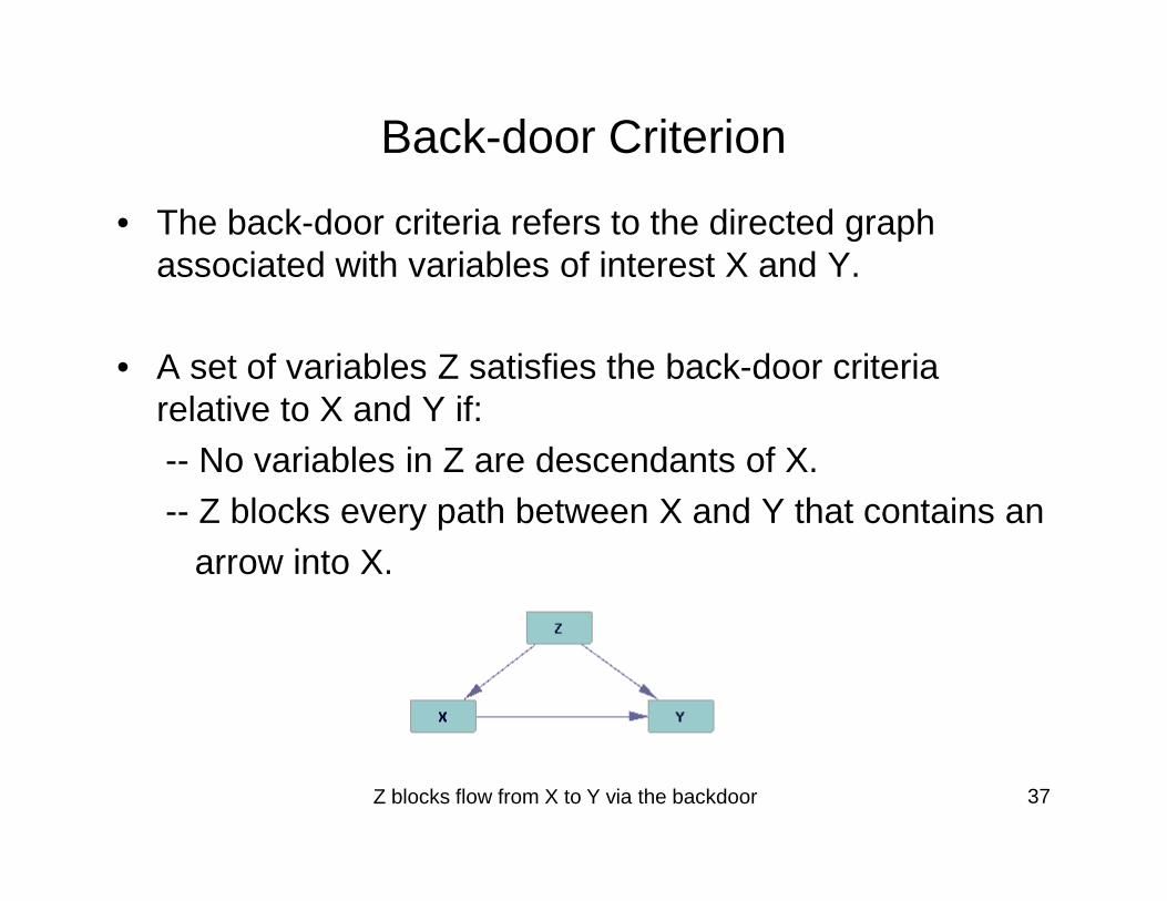
• The back-door criteria refers to the directed graph associated with variables of interest X and Y.

• A set of variables Z satisfies the back-door criteria relative to X and Y if:-- No variables in Z are descendants of X.

37

-- No variables in Z are descendants of X.-- Z blocks every path between X and Y that contains an

arrow into X.

Z blocks flow from X to Y via the backdoor

OLS works to block the back-doorGiven we can observe Z in the previous slide, we can run ols regression of Y on X and Z. The coefficient associated with X will be an unbiased and consistent estimate of ∂Y/∂X. We have blocked the back door by conditioning on Z.

__________Note in the previous slide we have omitted error terms and have assumed these to be simple parents of each variable (one for each X,Y and Z) and not correlated amongst themselves. If such correlations exist

38

each variable (one for each X,Y and Z) and not correlated amongst themselves. If such correlations exist we can deal with unbiased and consistent estimation using instrumental variables, as discussed below.

OLS refers to Ordinary Least Squares, which is more properly titled “Classical Least Squares,” as there is nothing “ordinary” about it. Classical Least Squares was discovered by Carl Friedrich Gauss (see Stephen M Stigler, 1986, The History of Statistics, The Measurement of Uncertainty before 1900, page 140-143, Cambridge, MA: Harvard University press).

Finally, note that the piecemeal approach to causal identification which we discussed above with respect to causal sufficiency, will now carry over to parameter estimation. That is we do not advocate large systems estimators, but rather focus (and advocate generally) consistent estimation (and understanding) of individual coefficients.

Front Door Criterion

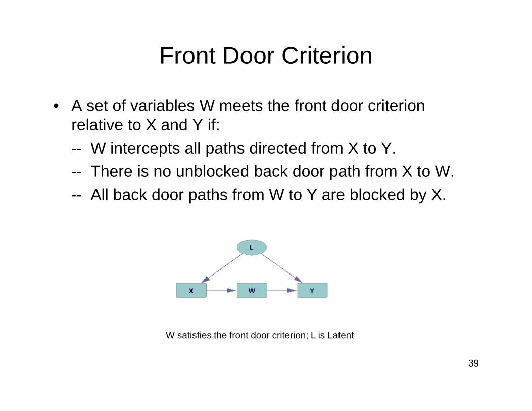
• A set of variables W meets the front door criterion relative to X and Y if:-- W intercepts all paths directed from X to Y.-- There is no unblocked back door path from X to W.-- All back door paths from W to Y are blocked by X.

39

W satisfies the front door criterion; L is Latent

OLS in two steps works for the front door identification

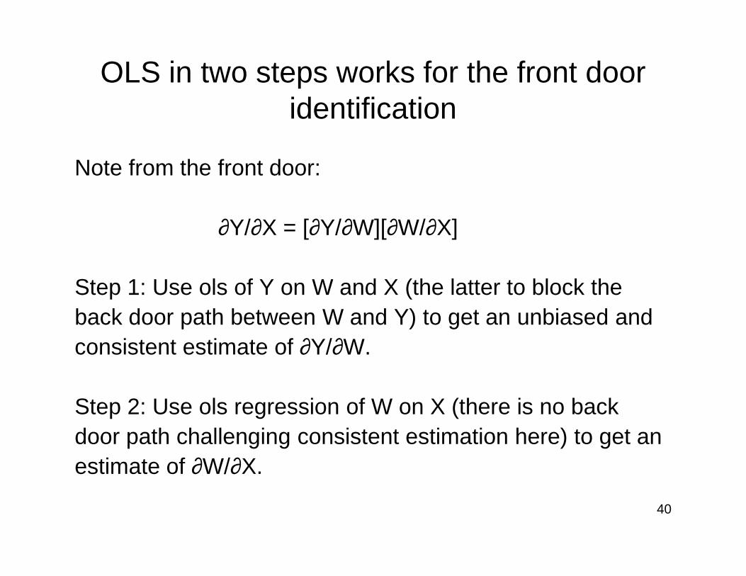
Note from the front door:

∂Y/∂X = [∂Y/∂W][∂W/∂X]

Step 1: Use ols of Y on W and X (the latter to block the

40

Step 1: Use ols of Y on W and X (the latter to block the back door path between W and Y) to get an unbiased and consistent estimate of ∂Y/∂W.

Step 2: Use ols regression of W on X (there is no back door path challenging consistent estimation here) to get an estimate of ∂W/∂X.

Instrumental Variables

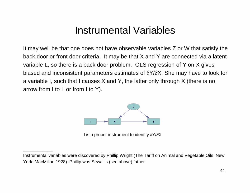
It may well be that one does not have observable variables Z or W that satisfy the back door or front door criteria. It may be that X and Y are connected via a latent variable L, so there is a back door problem. OLS regression of Y on X gives biased and inconsistent parameters estimates of ∂Y/∂X. She may have to look for a variable I, such that I causes X and Y, the latter only through X (there is no arrow from I to L or from I to Y).

41

______Instrumental variables were discovered by Phillip Wright (The Tariff on Animal and Vegetable Oils, New York: MacMillan 1928). Phillip was Sewall’s (see above) father.

I is a proper instrument to identify ∂Y/∂X

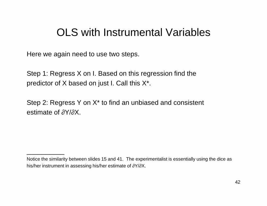
OLS with Instrumental Variables

Here we again need to use two steps.

Step 1: Regress X on I. Based on this regression find the predictor of X based on just I. Call this X*.

Step 2: Regress Y on X* to find an unbiased and consistent

42

Step 2: Regress Y on X* to find an unbiased and consistent estimate of ∂Y/∂X.

__________Notice the similarity between slides 15 and 41. The experimentalist is essentially using the dice as his/her instrument in assessing his/her estimate of ∂Y/∂X.

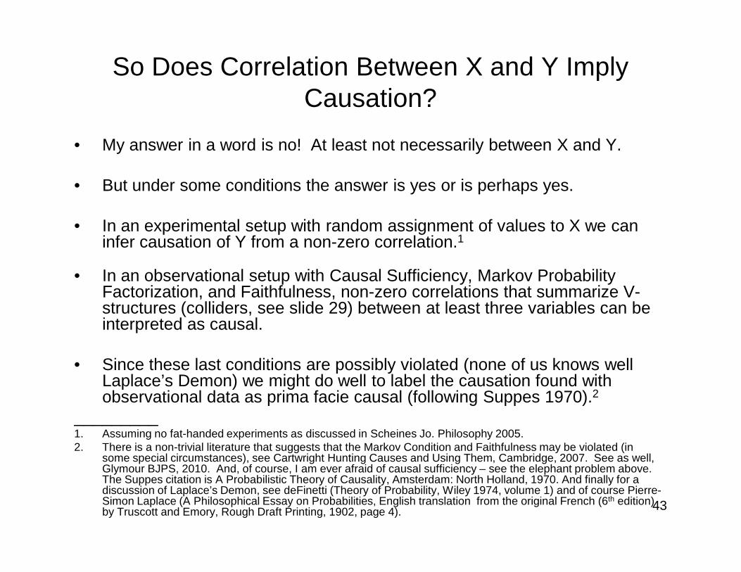
So Does Correlation Between X and Y Imply Causation?

• My answer in a word is no! At least not necessarily between X and Y.

• But under some conditions the answer is yes or is perhaps yes.

• In an experimental setup with random assignment of values to X we can infer causation of Y from a non-zero correlation.1

• In an observational setup with Causal Sufficiency, Markov Probability Factorization, and Faithfulness, non-zero correlations that summarize V-

43

Factorization, and Faithfulness, non-zero correlations that summarize V-structures (colliders, see slide 29) between at least three variables can be interpreted as causal.

• Since these last conditions are possibly violated (none of us knows well Laplace’s Demon) we might do well to label the causation found with observational data as prima facie causal (following Suppes 1970).2

_________1. Assuming no fat-handed experiments as discussed in Scheines Jo. Philosophy 2005.2. There is a non-trivial literature that suggests that the Markov Condition and Faithfulness may be violated (in

some special circumstances), see Cartwright Hunting Causes and Using Them, Cambridge, 2007. See as well, Glymour BJPS, 2010. And, of course, I am ever afraid of causal sufficiency – see the elephant problem above. The Suppes citation is A Probabilistic Theory of Causality, Amsterdam: North Holland, 1970. And finally for a discussion of Laplace’s Demon, see deFinetti (Theory of Probability, Wiley 1974, volume 1) and of course Pierre-Simon Laplace (A Philosophical Essay on Probabilities, English translation from the original French (6th edition) by Truscott and Emory, Rough Draft Printing, 1902, page 4).

Thanks to, among others:

44

A Few References

• Pearl, Judea. “Causal Diagrams for Empirical Research,” Biometrika, 1995

• Pearl, Judea. Causality, Models Reasoning and Inference, New York: Cambridge University Press, 2000, 2009

45

• Spirtes, Glymour and Scheines, Causation, Prediction and Search, New York: Springer-Verlag, 1993 (and MIT Press, 2000).

• Glymour and Cooper, Computation, Causation and Discovery, MIT Press, 1999.

Thanks, David

46

Todd and David near the top of Pacaya Volcano in Guatemala, May 2009

Pacaya Volcano in Guatemala, May 2010