Page 1
Final Report
FWHA/INDOT/JTRP-2006/23
CORRIDOR MAPPING USING AERIAL TECHNIQUE
By
James S. Bethel Professor of Civil Engineering
Boudewijn H.W. van Gelder
Professor of Civil Engineering
Ali Fuat Cetin Graduate Research Assistant
and
Aparajithan Sampath
Graduate Research Assistant
School of Civil Engineering Purdue University
Joint Transportation Research Program
Project No: C-36-17RRR File No: 8-4-70
SPR-2851
Conducted in Cooperation with the Indiana Department of Transportation and the
U.S. Department of Transportation Federal Highway Administration
The contents of this report reflect the views of the authors, who are responsible for the facts and the accuracy of the data presented herein. The contents do not necessarily reflect the official views or policies of the Indiana Department of Transportation or the Federal Highway Administration at the time of publication. The report does not constitute a standard, specification, or regulation.
Purdue University West Lafayette, IN 47907
August 2006
Page 2
TECHNICAL REPORT STANDARD TITLE PAGE 1. Report No. FHWA/IN/JTRP-2006/23
2. Government Accession No. 3.Recipient’s Catalog No.
5.Report Date August 2006
4. Title and Subtitle
Corridor Mapping Using Aerial Lidar Technique 6.Performing Organization Code
7. Author(s) James S. Bethel, Boudewijn H.W. van Gelder, Ali Fuat Cetin, Aparajithan Sampath
8. Performing Organization Report No. FWHA/INDOT/JTRP-2006/23
10. Work Unit No.
9. Performing Organization Name and Address Joint Transportation Research Program School of Civil Engineering Purdue University 550 Stadium Mall West Lafayette, IN 47907-2051
11. Contract or Grant No. SPR-2851
13. Type of Report and Period Covered Final Report
12. Sponsoring Agency Name and Address Indiana Department of Transportation State Office Building 100 North Senate Avenue Indianapolis, IN 46204
14. Sponsoring Agency Code
15. Supplementary Notes 16. Abstract With properly designed LIDAR control, assessment of 3D as-builts is attainable with an average over-all horizontal (planimetric) error of 0.324 ft (9.9 cm). Specifically, with an RMS error of 0.284 ft (8.7 cm) in Northing, and 0.255 ft (7.8 cm) in Easting. The average over-all vertical (height) error is 0.003 ft (0.1 cm) with a 0.108 ft (3.3 cm) RMS error. Lidar recognizable control (2m x 2m chevrons) was spaced at approximately 200m parallel to the direction of the axis of the project corridor, and at 60m sideway intervals. The project corridor was about 6 km long. Least Squares Image matching software was developed. The internal accuracy proved to be 0.027 ft (8mm). The strip width was approximately 111m and overlap between the Lidar strips changes from 55 to 90m sideways. Each flight line was flown twice in opposite directions showing 55 % overlap in two strips and 75 % in other two. The overall conclusion about the usage of Lidar aerial surveys for corridor mapping projects is that this technique is an efficient, cost cutting alternative to classical terrestrial and aerial survey techniques. However, at this point of the research it is felt that that the design of the LiDAR control plays a critical role to the success of the deployment of aerial LiDAR surveys. Augmentation of ground-based LiDAR and classical surveys proves necessary because of shielding of the airborne laser signals (e.g. underpasses). Comparison of the Lidar based model against the photogrammetric model obtained from low flying aerial photography (helicopter) should be made once the latter model becomes available. 17. Keywords Airborne Lidar, Accuracy Assessment, Edge of Pavement Feature Extraction, Evaluation
18. Distribution Statement
19. Security Classf. (of this report)
20. Security Classf. (of this page)
21. No. Of Pages 89
22. Price
Page 3
i
TABLE OF CONTENTS
PAGE LIST OF TABLES............................................................................................................. iii LIST OF FIGURES ........................................................................................................... iv CHAPTER 1: INTRODUCTION........................................................................................1
1.1. Background..........................................................................................................1 1.2. Airborne Laser Scanners......................................................................................2 1.3. Research Objectives and Methodology .............................................................10
CHAPTER 2: EVALUATION AND ADJUSTMENT OF LIDAR DATA......................16 2.1. Error Sources .....................................................................................................16 2.2. Data Description ................................................................................................28 2.3. Least Squares Location Model ..........................................................................34 2.4. Adjusting the Uncalibrated Data .......................................................................42
CHAPTER 3: EDGE OF PAVEMENT EXTRACTION AND EVALUATION .............43 3.1. Highway Cross-Section Elements .....................................................................46 3.2. Feature Extraction..............................................................................................49
CHAPTER 4: FIELD TRIP TO ODOT.............................................................................63 CHAPTER 5: CONCLUSIONS ........................................................................................69 APPENDIX A: CONTROL COMPARISION UNADJUSTED .......................................74 APPENDIX B: CONTROL COMPARISION ADJUSTED .............................................77 APPENDIX C: ELEVATION COMPARISION W/CALIBRATED DATA ...................80 APPENDIX D: CONTROL POINT COMPARISION FOR EACH STRIP.....................82
Page 4
ii
LIST OF TABLES PAGE
Table 2.1: Planimetric Comparison of Lidar Data with GPS Surveyed Control Points ... 38 Table 2.2: Control Point Comparison in Horizontal Coordinates..................................... 40 Table 3.1: Comparison of New "High Resolution" Spaceborne and Airborne Remote Sensing Technologies........................................................................ 24
Page 5
iii
LIST OF FIGURES PAGE
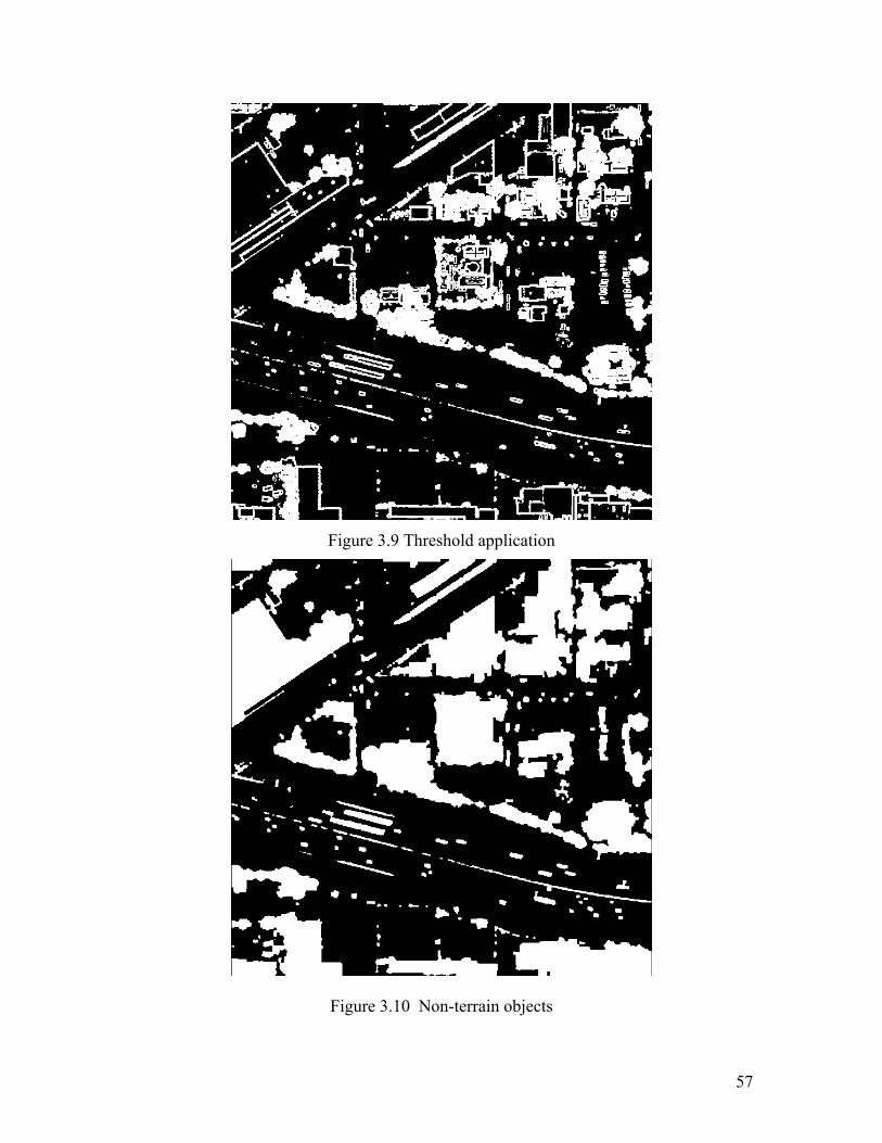
Figure 1.1: A Typical Lidar System Sensor Configuration ............................................... 3 Figure 2.1: Sensor Configuration of Airborne Lidar Systems ......................................... 22 Figure 2.2: Boresight Induced Errors................................................................................ 23 Figure 2.3: Scanner Induced Errors ................................................................................. 24 Figure 2.4: Illustration of the Effects of Terrain Slope on Observable Elevation Error .. 27 Figure 2.5: Project Area ................................................................................................... 28 Figure 2.6: Flight Paths and Control Points...................................................................... 29 Figure 2.7: Lidar Detectable Targets ................................................................................ 30 Figure 2.8: Painting Lidar Detectable Targets.................................................................. 32 Figure 2.9: Dataset with Point Spacing for a Lidar Flight Line, Along the two Opposing Flight Directions............................................................................. 32 Figure 2.10: Final Oupout as a Lidar Intensity Image from Operator-Adjusted Data...... 33 Figure 2.11: Lidar Intensity and Depth Image of a Portion of the Study Area with a 3D View ..................................................................................................... 33 Figure 2.12: Template and the Target in the Intensity Image for LSM............................ 34 Figure 2.13: One of the Control Points in the Intensity Range......................................... 37 Figure 2.14: Least Squares Image Matching of Control Points........................................ 38 Figure 2.15: Errpr Distribution for Operator-Calibrated Data.......................................... 40 Figure 2.16: Lidar Points around the Control Point 267................................................... 44 Figure 2.17: Lidar Data Strips Showing the Overlaps and the Directions........................ 41 Figure 2.18: Error Directions due to Boresight Misalignment ......................................... 41 Figure 3.1: Intensity Image Used for Clustering ............................................................. 50 Figure 3.2: Clustering Results .......................................................................................... 51 Figure 3.3: Closer Look at the Clustered Image .............................................................. 51 Figure 3.4: Intensity Image for Stnadard Deviation Filter ............................................... 53 Figure 3.5: Standard Deviation Filter Applied Intensity Image ...................................... 54 Figure 3.6: Entropy Filter Applied Intensity Image.......................................................... 55 Figure 3.7: Height Image ................................................................................................. 55 Figure 3.8: Standard Deviation Filter Applied Height Image .......................................... 56 Figure 3.9: Threshold Application ................................................................................... 57 Figure 3.10: Non-Terrain Objects..................................................................................... 57 Figure 3.11: Bare Earth Pixels .......................................................................................... 58 Figure 3.12: Intensity Image Without Non-Terrain Objects ............................................ 59 Figure 3.13: Clustered Image Showing Road Surfaces ................................................... 59 Figure 3.14: Separated Road Surfaces .............................................................................. 60 Figure 3.15: Opening and Closing Operation on Road Surfaces ..................................... 60 Figure 3.16: Road Surfces over Intensity Image ............................................................. 61 Figure 3.17: Application of Canny Edge Detection over Road Surfaces ......................... 61 Figure 4.1: Cessna Grand Caravan :Lidar Instrumentation .............................................. 64 Figure 4.2: Scenes from the Project Area Produced using QT Modeler with Elevation Values ........................................................................................... 67 Figure 4.3: Scenes from the Project Area Produced Using QT Modelier with Intensity Values ............................................................................................. 68
Page 6
1
CHAPTER 1
INTRODUCTION
1.1 BACKGROUND
Accurate terrain mapping is important for highway corridor planning and design,
environmental impact assessment, and infrastructure asset management. The management
of transportation infrastructure assets can be more efficient and cost-effective by using a
geographical information system (GIS) for defining georeferenced locations, storing
attribute data, and displaying data on maps. Collecting good-quality geographical
coordinate data by traditional ground-based manual methods may require a substantial
investment depending upon the size of the assets. In the case of natural or orchestrated
disasters, the assessment of damage and re-building can be costly and time-consuming if
the inventory and terrain model data are not easily available. Safe and efficient mobility
of goods and people requires periodic monitoring and maintenance of all transportation
infrastructure components within the right-of-way including the following: pavements,
bridges, tunnels, interchanges, roadside safety structures, and drainage structures. These
data collection activities require time- and labor-intensive efforts. In many parts of the
world, highway data are collected at highway speed using non-contact photography,
video, laser, acoustic, radar, and infrared sensors. These terrestrial non-contact
technologies may suffer limitations resulting from time of day, traffic congestion, and
proximity to urban locations. Additionally, traditional terrestrial ground surveys can be
quite hazardous, especially in the areas of maintenance work zones. Modern airborne and
Page 7
2
spaceborne remote-sensing technologies offer cost-effective terrain mapping, inventory,
and monitoring data collection [115].
Recently Airborne Laser Scanning (ALS) systems are preferred more and more for
collecting topographic data since it provides quick and accurate data for large areas.
Laser scanning systems available on the market are presently in a fairly mature state of
art, where most of technical hardware difficulties and system integration problems have
been solved. The systems are very complex, being more a ‘geodetic’ system on the data
acquisition part and more a ‘photogrammetric’ system on the data processing part. What
very much remains is the development of algorithms and methods for interpretation and
modeling of laser scanner data, resulting in useful representations and formats for an end-
user [100].
1.2 AIRBORNE LASER SCANNERS
Airborne laser mapping is an emerging technology in the field of remote sensing that is
capable of rapidly generating high-density, geo-referenced digital elevation data with an
accuracy equivalent to traditional land surveys but significantly faster than traditional
airborne surveys.
Airborne laser mapping offers lower field operation costs and post-processing costs
compared to traditional survey methods. Point for point, the cost to produce the data is
significantly less than other forms of traditional topographic data collection making it an
Page 8
3
attractive technology for a variety of survey applications and data end-users requiring low
cost, high-density, high accuracy geo-referenced digital elevation data.
Airborne laser mapping use a combination of three mature technologies; rugged compact
laser rangefinders (LIDAR), highly accurate inertial reference systems (INS) and the
global positioning satellite system (GPS) (Figure 1.1) . By integrating these subsystems
in to a single instrument mounted in a small airplane or helicopter, it is possible to rapidly
produce accurate digital topographic maps of the terrain beneath the flight path of the
aircraft.
Figure 1.1 A typical LIDAR system sensor configuration
Page 9
4
The absolute accuracy of the elevation data is 15 cm; relative accuracy can be less than 5
cm. Absolute accuracy of the XY data is dependent on operating parameters such as
flight altitude but is usually 10's of cm to 1 m.
The elevation data is generated at 1000s of points per second, resulting in elevation point
densities far greater than traditional ground survey methods. One hour of data collection
can result in over 10,000,000 individually geo-referenced elevation points. With these
high sampling rates, it is possible to rapidly complete a large topographic survey and still
generate DTMs with a grid spacing of 1 m or less.
The technology allows for extremely rapid rates of topographic data collection. With
current commercial systems it is possible to survey one thousand square kilometers in
less than 12 hours and have the geo-referenced DTM data available within 24 hours of
the flight. A 500 kilometer linear corridor, such as a section of coastline or a transmission
line corridor can be surveyed in the course of a morning, with results available the next
day.
Airborne laser mapping instruments are active sensor systems, as opposed to passive
imagery such as cameras. Consequently, they offer advantages and unique capabilities
when compared to traditional photogrammetry. For example, airborne laser mapping
systems can penetrate forest canopy to map the floor beneath the treetops, accurately map
the sag of electrical power lines between transmission towers or provide accurate
elevation data in areas of low relief and contrast such as beaches.
Page 10
5
Airborne laser mapping is a non-intrusive method of obtaining detailed and accurate
elevation information. It can be used in situations where ground access is limited,
prohibited or risky to field crews.
Commercial airborne laser mapping systems are now available from several instrument
manufacturers while various survey companies have designed and built custom systems.
Similar to aerial cameras, the instruments can be installed in small single or twin-engine
planes or helicopters. Since the instruments are less sensitive to environmental conditions
such as weather, sun angle or leaf on/off conditions, the envelope for survey operations is
increased. In addition, airborne laser mapping can be conducted at night with no
degradation in performance.
A number of service providers are operating these instruments around the world, either
for dedicated survey needs or for hire on a project basis. Some organizations are starting
to survey areas on speculation and then offering the laser-generated data sets for resale
similar to the satellite data market.
1.2.1 The Technology
While the core technologies for airborne laser mapping have been in development for the
past 25 years, the commercial market for these instruments has only developed
significantly within the last five years. This commercial development has been driven by
the availability of rugged, low-cost solutions for each of the core subsystems and the
growing demand for cheap, accurate, timely, digital elevation data.
Page 11
6
In operation, a pulsed laser rangefinder mounted in the aircraft accurately measures the
distance to the ground by recording the time it takes a laser pulse to reflect back to the
aircraft from the ground or from objects such as buildings, trees or power lines. Since the
speed of light is known, the elapsed time is converted to an accurate distance or slant
range. Some instruments record multiple returns from a single laser pulse to capture a
vertical profile along the slant range. A scanning or rotating mirror is used to provide
coverage across the path of the aircraft with swath widths dependent on scan angle and
operating altitude. Simultaneously the INS subsystem records the roll, pitch and heading
of the aircraft to determine its orientation in space, while the GPS subsystem provides the
precise location of the aircraft through a differential kinematic solution. During post-
processing the INS orientation and GPS position solutions are combined with the laser
slant ranges to calculate accurate XYZ co-ordinates for each laser return.
The technology does not provide a real-time solution; it requires additional post-
processing after the field operations and data collection are completed to generate the
final XYZ data points. Post-processing is based on proprietary software developed by
each instrument manufacturer but has significantly faster turn-around times than
conventional survey techniques, on the order of 10's of hours compared to 10's days for
traditional methods.
In addition to directly generating digital XYZ data points, post-processing software
modules for the automatic analysis and classification of various features are being
developed. Software modules already exists for such activities as vegetation classification
Page 12
7
and removal while other modules are being developed for automatic feature extraction,
building recognition or automatic power wire detection and modeling.
1.2.2 Applications
Depending on the application, airborne laser mapping technology is either a
complementary or a competitive technology when compared to existing survey methods.
For many survey applications airborne laser technology is currently deployed in
conjunction with other more traditional sensors including standard aerial cameras, digital
cameras, multispectral scanners or thermal imagers. However, in certain applications,
such as forestry or coastal engineering, it offers capabilities not achievable with any other
technology.
The most active application areas are:
1. DTM Generation for a Variety of GIS/Mapping Related Products.
Airborne laser mapping is a rapid, cost-effective source of high-accuracy, high-density
elevation data for many traditional topographic mapping applications. The technology
allows large area topographic surveys to be completed significantly faster and at a
reduced cost compared to traditional survey methods.
2. Forestry.
The use of airborne laser mapping in the forestry industry was one of the first commercial
areas investigated. Accurate information on the terrain and topography beneath the tree
canopy is extremely important to both the forestry industry and natural resource
Page 13
8
managers. Accurate information on tree heights and densities is also critical information
that is difficult to obtain using conventional techniques. Airborne laser technology, unlike
radar or satellite imaging, can simultaneously map the ground beneath the tree canopy as
well as the tree heights. Post-processing of the data allows the individual laser returns to
be analyzed and classified as vegetation or ground returns allowing DTMs of the bare
ground to be generated or accurate representative tree heights to be calculated.
Consequently, airborne laser mapping is an extremely effective technique for forestry
companies when compared to photogrammetry or extensive ground surveys.
3. Coastal Engineering.
This is another area where airborne laser technology offers state-of-the-art type
performance with significant advantages over other survey techniques. Since traditional
photogrammetry is difficult to use in areas of limited contrast, such as beaches and
coastal zones, an active sensing technique such as airborne laser mapping offers the
ability to complete surveys that would be too costly to contemplate using other methods.
In addition, highly dynamic environments such as coastal zones often require constant
updating of baseline survey data. Airborne laser mapping offers a cost-effective method
to do this on a routine basis. It is also used for mapping and monitoring of shore belts,
dunes, dikes and coastal forests.
4. Corridor or Right-of-Way Mapping.
Airborne laser mapping allows rapid, cost-effective, accurate mapping of linear corridors
such as power utility right-of-ways, gas pipelines, or highways. A major market is
Page 14
9
mapping power line corridors to allow for proper modeling of conductor catenary curves,
sag, ground clearance, encroachment and accurate determination of tower locations. For
example data acquired through airborne laser surveys can be combined with simultaneous
measurements of air and conductor temperature and load currents to establish admissible
increases in load-carrying capacity of power lines.
5. Construction.
Timely and accurate digital, geo-referenced elevation data is useful in a variety of
construction and engineering activities. Examples include highway corridors, open-pit
mines or daily surveying of large construction sites.
6. Flood Plain Mapping
Accurate and updated models of flood plains are critical both for disaster planning and
recovery and flood insurance purposes. Airborne laser mapping offers a cost-effective
method of acquiring the topographic data required as input for various flood plain
modeling programs.
7. Urban Modeling.
Accurate digital models of urban environments are required for a variety of applications
including telecommunications, wireless communications, law enforcement and disaster
planning. An active remote sensing system such as a laser offers the ability to accurately
map urban environments without shadowing.
8. Disaster Response and Damage Assessment.
Page 15
10
Major natural disasters such as hurricanes or earthquakes stress an emergency response
organization’s abilities to plan and respond. Airborne laser mapping allows timely,
accurate survey data to be rapidly incorporated directly in to on going disaster
management efforts and allows rapid post-disaster damage assessments. It is particularly
useful in areas prone to major topographic changes during natural disasters; areas such as
beaches, river estuaries or flood plains.
9. Wetlands and Other Restricted Access Areas
Many environmentally sensitive areas such as wetlands offer limited ground access and
due to vegetation cover are difficult to asses with traditional photogrammetry. Airborne
laser mapping offers the capability to survey these areas. The technology can also be
deployed to survey toxic waste sites or industrial waste dumps.
Since airborne laser mapping is a relatively new technology, applications are still being
identified and developed as end-users start to work with the data. There are on going
efforts to identify areas where this technology allows value-added products to be
generated or where it offers significant cost reductions over traditional survey methods
[118].
1.3 RESEARCH OBJECTIVES AND METHODOLOGY
LIDAR (LIght Detection And Ranging) systems are complex multi-sensory systems and
incorporate at least three main sensors, GPS and INS navigation sensors, and the laser-
scanning device. The complexity of the system results in possible error sources that can
Page 16
11
degrade the accuracy of the acquired LIDAR data. The errors in laser scanning data can
come from individual sensor calibration or measurement errors, lack of synchronization,
or misalignment between the different sensors [101]. [102] presents an overview of basic
relations and error formulas concerning airborne laser scanning.
As laser scanners have a potential range accuracy of better than 1 dm, the position and
orientation system (POS) should allow at least one order of magnitude better accuracy.
Such accuracy can be achieved only by an integrated POS consisting of a DGPS and an
inertial measurement unit (IMU)/INS. After a surveying flight, basically two data sets are
available: the POS data and the laser ranges with the instantaneous scanning angles.
Assuming that the accuracy of POS data is better than 1 dm in position and 0.028 in
orientation, already very precise laser measurement points in an earth-fixed coordinate
system can be calculated. However, some systematic parameters must be considered.
These are e.g., the three mounting angles of the laser scanner frame, described by the
Euler angles roll, pitch and yaw, with respect to the platform-fixed coordinate system
usually with origin at the IMU, the position of the laser scanner with respect to the IMU,
and the position of the IMU with respect to the GPS. This so-called calibration data can
be derived from laser scanner surveys, whereby certain reference areas are flown-over in
different directions. Reference areas are e.g., flat terrain like large sport fields or
stadiums, buildings and corner of buildings. From the relative orientation and position of
the different surveys and their absolute orientation and position with respect to an earth-
fixed coordinate system, calibration data can be derived [103].
Page 17
12
Each component requires calibration and the offsets between the components needs to be
determined. GPS/INS and range finders are usually calibrated in the lab; thus this
research will concentrate on scanner and misalignment (bore sight) values. The
misalignment between the INS system and the scanner is the largest source of systematic
error in an ALS and must be addressed before the sensor can be effectively deployed. It
has been observed empirically that these misalignment errors are often relatively small
(0.1 – 3 degrees), but their effect on the recorded ground points will depend on flying
height and the scanner field of view (maximum scan angle) [104].
Most of these errors are systematic and can be corrected. To eliminate the effect of the
systematic errors, several procedures have been proposed so far. One group can be
categorized as data driven. The motivation is to correct the laser points by transforming
them so that the difference between their values and the reference control information is
minimized. Another approach is based on recovering the systematic system errors.
Several authors report recovering the errors by conducting different flight patterns over
flat, locally horizontal surfaces and “flattening" the surface as a function of the
systematic errors. Others base their calibration procedure on control, height, and tie
points, in a fashion similar to photogrammetric block adjustment, or propose to
reconstruct the elevation model around distinct landmarks to tie the overlapping strips
which is called strip adjustment [110].
Page 18
13
Although many systems require the calibration for each survey flight there are also some
other systems [112] claiming no need for any calibration except any major component
replacement.
Currently the most common method of calibrating an ALS sensor is also the least
rigorous: profiles of overlapping strips are compared and an experienced operator
manually adjusts the misalignment angles until the strips appear to visually fit. Although
pragmatic, this approach is time consuming and labor intensive; and the results do not
immediately provide any statistical measure on the quality of the calibration.
Several strip adjustment models have been proposed by [104], [105], [106], [107], [108],
[109], [111]. All of these strip adjustment methods are based on the observed vertical or
three-dimensional discrepancies between the overlapping LIDAR strips. Systematic
planimetric errors are often much larger than height errors of the LIDAR data, and
therefore, a three-dimensional strip adjustment is the desirable solution. Some of the strip
adjustment methods work only with tie points (without any ground control information),
however, the use of some type of ground control is desirable, since eliminating the
relative discrepancies between overlapping strips does not provide an absolute check of
the dataset. Applications demanding the highest accuracy require the elimination of
absolute errors, which cannot be achieved without the use of absolute control
information. Ground control information can be used in the strip adjustment process or
after strip adjustment to correct the remaining absolute errors in the corrected strips.
Many times after the strip adjustment, a horizontal surface with a known elevation is used
Page 19
14
to correct remaining vertical shifts in the data. However, remaining absolute errors after
strip adjustment can be more complex than just a vertical shift. Three-dimensional
ground control information, buildings, known roof structures, etc., are often used.
However, this type of control information is not always available. Furthermore, due to the
characteristics of laser data, the identification of distinct points of buildings and roof
structures in LIDAR data can result in a biased position, which could affect the accuracy
of the corrected LIDAR data. Therefore, for applications with high accuracy
requirements, such as corridor mapping, well-identifiable LIDAR-specific ground control
targets are necessary [101].
Accurate terrain data is needed for highway corridor mapping and relocating existing or
locating new infrastructures. Besides, the data should be collected in as fast as possible
considering the personnel safety issues. Currently traditional field surveying and
photogrammetric mapping processes require early collection and processing of data for
design purposes. However the accuracies provided by these methods may be needed at
the final stages of the process and they require too much time and cost. Lidar technology
can provide data at the required accuracy level for early stages of the process. The current
research aims to achieve the required accuracy level for the final stages of the design
process. Currently Lidar data vendors specify a height precision of 15 cm and above 50
cm horizontal accuracies for their systems.
For the last few years it has been shown in many research papers that automated feature
extraction from Lidar data is a very promising issue. However achieving the required
Page 20
15
accuracies for design stages using the automated technologies is a challenging issue. But
the quality and the quantity of the Lidar data may provide a high accuracy 3D feature
extraction environment.
In this research we used a novel approach which uses LIDAR detectable ground control
targets. “L” shaped targets are used along the strips in the project area which were
applied by painting the inside of a template. This proposal describes the matching of the
targets in the LIDAR intensity images using Least Squares Image Matching (LSIM)
technique and the least squares method to remove the systematic errors from the un-
calibrated data set.
Highway corridor mapping is an important task for most DOTs in the U.S. which is
mainly done for evaluation of the existing infrastructure. In this research, the edge of
pavements on the roads will be extracted from the Lidar data and the accuracy for the
extracted features along the project area will be compared with the ones derived from
aerial photogrammetry, and ground total station.
The report is organized as follows. The next section describes the error budget for Lidar
technology, a brief description of the least squares image matching technique, test results
and adjustment method for misalignment correction. The following section describes
feature extraction for highway edge of pavements, and comparison of the extracted
features using the all three methods mentioned above.
Page 21
16
CHAPTER 2
EVALUATION AND ADJUSTMENT OF LIDAR DATA
One of the goals of the project is to evaluate the planimetric and the vertical accuracy, as
well as the internal consistency of the lidar data. However, the nature of lidar data
collection made it challenging to device a strategy for such a task. Unlike
photogrammetry, Lidar technology does not generate continuous data. Therefore, it is
impossible to ensure that control points are directly scanned as it is not possible to point
the laser scanner to a particular spot, and then measure its coordinates. The point cloud is
a series of discrete, albeit very close, three dimensional coordinates. It was finally
decided that control points in the study area be painted such that they are visible in the
lidar dataset.
Before going into details of the analysis, the error sources in an airborne lidar system is
going to be presented.
2.1 ERROR SOURCES
Digital elevation models (DEMs) or triangulated irregular networks (TINs) produced
from lidar observations are created from lidar returns labeled as “ground” observations.
These lidar-derived “ground” elevations contain error from three categories of sources:
• elevation error from the sensor system measurement,
• horizontal error from the sensor system measurement, and
• labeling error process of identifying a “ground” return from other types of returns (e.g.,
canopy top, intermediate vegetation, building top).
Page 22
17
The error in the measured elevation of a lidar point is the cumulative product of the
sensor/platform sources, such as analysis of waveform, identification of the return
position in the pulse length, and position error in the GPS/INU control. Horizontal error
is a function of the same factors but often dominated by flying height. Horizontal error is
often reported to be approximately 1/1000th of the flying height AGL on most systems.
The horizontal error will introduce additional elevation error in the use of the
observations. The lidar “ground” return set contains both omission and commission
errors. Some points in the set are incorrectly labeled as “ground” returns, and some true
“ground” returns are omitted. From a user’s perspective, the point set is treated as if there
are no errors or occasionally as if there are only elevation errors. The use of lidar
observations typically involves the interpolation of an irregular point set to a DEM,
which may introduce additional elevation error. Finally, any assessment of elevation error
with reference data introduces additional “apparent” error from the surveying of the
reference data [119].
2.1.1 Sources of Positional (X-Y-Z) Error
The primary sources of positional error in the lidar collection process are associated with
the Global Positioning System (GPS) equipment onboard the aircraft, the inertial
navigation unit (INU) for estimating positions between GPS fixes, and the inertial
measurement unit (IMU) for monitoring the pointing direction of the laser. The
horizontal (X-Y) error is typically much greater than the vertical error. Assessing the
horizontal accuracy of lidar observations is also problematic. Conventional assessments
of horizontal error involve multiple over-flights over building corners with flat roofs.
Most lasers used in the commercial lidar sensors are similar and have a divergence from
0.2 to 0.33 mr. This divergence, along with scan angle and flying height, defines the lidar
Page 23
18
footprint (typically between 24 cm to 60 cm). Smaller footprints are more likely to pass
through breaks in forest canopy [119].
2.1.1.1 Range Errors
The range accuracy is the most complicated among the major accuracy factors. In
practice, however, if the necessary measures and precautions are taken, the contribution
of range errors to 3D coordinate errors is the minimum among the major error sources,
with the exception of low flying heights and small scan angles, where its relative
importance with respect to the total error budget increases [102]. Under normal operating
conditions the range error from a typical laser rangefinder that is properly calibrated can
be expected to be between 2" to 3". However, the atmosphere acts to distort the path of
the laser pulse as it travels to the target and back again, introducing a timing error that
needs to be corrected. These corrections become critical at higher altitudes. These
atmospheric affects are usually minimized but not eliminated by incorporating an
appropriate atmospheric model in the post-processing of the LiDAR data. A surveyor
needs to pay close attention as specified operational altitudes increase [120].
2.1.1.2 Position Errors
This depends mainly on the quality of the DGPS postprocessing. Other factors: GPS
hardware, GPS satellite constellation during flight, number, distribution and distance of
ground reference stations from (aircraft values of 10–100 km have been reported),
accuracy of offsets and misalignment between GPS and INS, and INS and laser scanner
(depending on the used computation method less information might be sufficient, e.g.,
offset between GPS and laser and misalignment between INS and GPS, or offset and
Page 24
19
misalignment between laser and INS), and the accuracy of the laser beam direction
scanner accuracy . The GPS error varies over time, but it is bounded (exceptions can
occur during GPS outage), and through integration of GPS with INS, the temporal
variability is smoothed [102]. It is important for surveyors to have a good understanding
of GPS-related errors that fall into several broad categories. Sources of error include
satellite geometry (PDOP), orbital biases, multipath, antenna phase center modeling,
integer resolution and atmospheric errors. Compounding some of these errors is the
operational distance from the ground GPS stations. It is important to remember that for
every GPS-related error source, a method can be employed to detect, eliminate or
minimize that error. In general, when properly taken into account and with proper project
planning, GPS error contributes on the order of 2" to 4" of position error to the final
product [120].
2.1.1.3 Orientation Errors
This depends on the quality of the INS, the INS frequency (i.e., interpolation error) , the
method of postprocessing and integration with the GPS. Heading accuracy in addition
depends on latitude. The effect of attitude errors on the 3D accuracy increases with the
flying height and the scan angle [102]. Knowing the correct orientation or pointing
direction of the Lidar sensor is necessary for calculating an accurate spot location on the
ground. In practice, the orientation of the platform is recorded by an on-board inertial
measurement unit (IMU)/INS that is hard mounted to the Lidar sensor. While a variety of
IMUs are available commercially, a typical specification for the price/performance levels
common in most commercial Lidar sensors would be 0.005° pitch/roll, 0.008° heading
(POS/AV 510 from Applanix, Richmond Hill, Ontario, Canada post-processed solution)
Page 25
20
although some systems perform to a 0.0025° pitch/roll accuracy. A 0.005° angular error
corresponds to a 0.87 foot error from 10,000 feet and a 1.70 foot error from 20,000 feet.
However, there are additional contributions to the angular pointing error including
contributions from the scanning subsystem. Many of these additional errors can be
minimized but not eliminated by proper system calibration prior to data collection and
proper system modeling during post-processing.
2.1.1.3.1 Boresight Misalignment
Figure 2.1 shows the usual sensor configuration of airborne LIDAR systems. The
navigation sensors are separated the most since the GPS antenna is installed on the top of
the fuselage while the INS sensor is attached to the LIDAR system, which is down in the
aircraft. The spatial relationship between the sensors should be known with high
accuracy. In addition, maintaining a rigid connection between the sensors is also very
important since modeling any changes in the sensor geometry in time just would further
increase the complexity of the system model and thus may add to the overall error. The
INS frame is usually considered as the local reference system; thus the navigation
solution is computed in this frame. The spatial relationship between the laser scanner and
the INS is defined by the offset and rotation between the two systems. The critical
component here is the rotation since the object distance amplifies the effect of an angular
inaccuracy, while the effect of an inaccuracy in the offset does not depend on the flying
height. The description of the effects of the different boresight misalignment angles is
omitted here; for details see e.g. ([102]).
The coordinates of a laser point are a function of the exterior orientation of the laser
sensor and the laser range vector. The observation equation is:
Page 26
21
To obtain the local object coordinates of a LIDAR point, the laser range vector has to be
reduced to the INS system by applying the shift and rotation between the two systems,
which results in the coordinates of the LIDAR point in the INS system. The GPS/INS-
based navigation provides the orientation of the INS frame, including position and
attitude; thus the mapping frame coordinates can be subsequently derived. In our
discussion, the automated determination of the rotation component, the boresight matrix
between the INS and the laser frame, is addressed.
The boresight rotation can be described by three rotation angles, ω rotation around the x-
axis, ϕ rotation around the y-axis, and κ around the z-axis in the laser sensor frame. The
approximate values of the three rotation angles between the INS and the laser frames are
known from the mechanical alignment. The actual angles differ slightly from these
nominal values. The boresight misalignment problem is to determine these three
misalignment angles. Any discrepancy in their values results in a misfit between the
LIDAR points and the ground surface; the calculated coordinates of the LIDAR points
are not correct. In case the ground surface is unknown, the effect of the misalignment can
be seen if different overlapping LIDAR strips are flown in different directions.
Page 27
22
Figure 2.1. Sensor configuration of airborne LIDAR systems
Boresight misalignment has to be determined to obtain correct surface from the LIDAR
data. The unknown boresight misalignment angles can be found with ground control or
without it by using overlapping LIDAR strips flown in different directions. Since the true
ground surfaces are not always available preference should be given to techniques that do
not require a priori knowledge of the surface [111].
The misalignment between the INS system and the scanner is the largest source of
systematic error in an ALS and must be addressed before the sensor can be effectively
deployed. It has been observed empirically that these misalignment errors are often
relatively small (0.1 – 3 degrees), but their effect on the recorded ground points will
depend on flying height and the scanner field of view (maximum scan angle). When
Page 28
23
comparing data from overlapping strips on an un-calibrated system, the effects of these
errors will be seen as in Figure 2.2.
Figure 2.2 Boresight Induced Errors
On systems using an oscillating scanner (such as the Leica ALS40 and the Optech
ALTM), additional errors can be visible when comparing strips (Figure 2.3).
These additional effects are caused by errors in the angle encoder. As the mirror
accelerates and decelerates across its swath, the angle encoder undergoes small amounts
of torsion. This torsion causes a small, but systematic misreading of the angle, which is
manifested by the ends of the scan rising too high or dropping too low. Due to the
systematic nature of this error, it can be modeled and removed during the calibration
process.
Page 29
24
Figure 2.3. Scanner Induced Errors
To determine the calibration parameters empirically, data from overlapping strips must be
collected. Alternatively, data from one strip can be compared to a known surface. The
misalignment errors and scanner errors described above are all correlated with the
direction of flight. If strips are flown in opposite directions, then the induced errors will
be maximized and more importantly de-correlated. This will allow for a least-squares
approach to the problem. [104].
2.1.1.4 Time Offsets
For accurate 3D positioning, orientation, position, and range are required to be taken at
the same time. If there is a time offset and this is not known precisely, it will cause a
variable error. The error increases with increasing change rate of the related
measurements, e.g., while a time offset between range and rotation angles can have a
Page 30
25
small effect for a calm flight (rotation angles remain fairly stable) , it can influence the
3D accuracy a lot for a turbulent flight [102].
Concluding, the total error consists of a variable part that is dependent on major
parameters like flying height, scan angle, terrain topography, and land cover referring to
object geometry and reflectivity and a constant part 5–10 cm in good cases that is
independent of the previous parameters, e.g., pulse detection accuracy, GPS accuracy,
etc.
2.1.2 Lidar Point Labeling Error
A single lidar pulse of approximately 200 cm in length is emitted toward a surface
location at some 10,000 to 70,000 times per second. Most lidar sensors record the return
energy as a waveform of multiple pulses, and then unique returns are identified (e.g., four
or five returns). In some instances, the magnitude of the pulse is also recorded and is
referred to as intensity. From this set of lidar returns, both automated and manual
methods are used to identify or label each return as a “ground” return, “vegetation”
return, “building” return, or other. This process is sometimes referred to as “vegetation
removal.” Automated methods are based on neighborhood operators that iteratively
identify the lowest points within each neighborhood and add them to a candidate set of
“ground” returns. Subsequent iterations refine the candidate set by adding additional
returns that are also “low” or exhibit some angular deflection from a surface modeled by
the current candidate set of points. The exact neighborhood operators and parameters
vary by lidar mapping vendor and are proprietary information [119].
Page 31
26
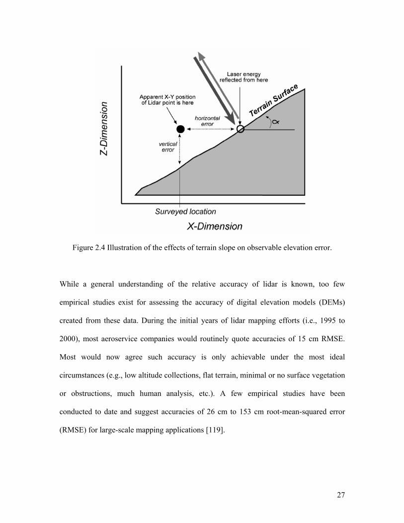
2.1.3 Mapping Sources of Error
A well-known characteristic of observed elevation error for terrain mapping is the
relationship with terrain slope. Even if the elevation of a surface observation is measured
without error, the horizontal error in the observation may introduce “apparent” error in
the elevation value from a user’s perspective. The introduction of elevation error based
on horizontal error is only true for inclined slopes (Figure 2.4). The maximum amount of
elevation error introduced is a function of surface slope: i.e.,
Elevation Error = tan α * Horizontal Displacement.
For instance, the additional elevation error introduced for a point with a 100-cm
horizontal error on a 10° slope can be up to ±18 cm. The maximum error will only occur
if the displacement is perpendicular to the contour line. The error will be zero for
displacement parallel with the contour. In practice, the displacement direction for any
single point is unknown and assumed to be random for the entire set of points. Early
work in topographic mapping has demonstrated the relationship between observation
point density and the accuracy of the derived DEM. As the density of observation points
increases, the accuracy of the resulting DEM increases. The density of lidar “ground”
returns depends on the nominal posting (i.e., spacing between lidar pulses at nadir), land-
cover type, and point-labeling approach. This density concept resulted in a maximum 5-m
posting criteria within FEMA’s guidelines for using lidar data to construct DEMs in the
floodplain mapping process. FEMA also suggested a minimum percentage of “data
voids,” areas where the distance to the nearest lidar observation is greater than some
threshold [119].
Page 32
27
Figure 2.4 Illustration of the effects of terrain slope on observable elevation error.
While a general understanding of the relative accuracy of lidar is known, too few
empirical studies exist for assessing the accuracy of digital elevation models (DEMs)
created from these data. During the initial years of lidar mapping efforts (i.e., 1995 to
2000), most aeroservice companies would routinely quote accuracies of 15 cm RMSE.
Most would now agree such accuracy is only achievable under the most ideal
circumstances (e.g., low altitude collections, flat terrain, minimal or no surface vegetation
or obstructions, much human analysis, etc.). A few empirical studies have been
conducted to date and suggest accuracies of 26 cm to 153 cm root-mean-squared error
(RMSE) for large-scale mapping applications [119].
Page 33
28
2.2. DATA DESCRIPTION
This research is funded by Joint Transportation Research Program (JTRP Project
Number: C-36-17RRR, File Number: 8-4-70, SPR-2851) for Indiana Department of
Transportation (INDOT) under the name of “Corridor Mapping Using Aerial Lidar
Technique”. The project area selected for this research is on an approximately 8 km
portion of I-70 highway in Marion County, Indiana as seen in Figure 2.5. 4 parallel flight
paths are used to get 8 strips having 4 flights in opposite directions (Figure 2.6). The strip
width was approximately 111m and the overlap between the strips changes from 55 to
90m. Figure 2.6 shows the flight paths and 73 ground control points used in the project.
Figure 2.5 Project Area
Data was collected by the service provider company using a Leica Geosystems ALS50
system on October 22, 2004. The data was collected with a 12 degree field of view at 70
Hz scan frequency, and 52.3 kHz pulse rate from an altitude of 610m. The point density
obtained for this area was 25 points/m² having approximately 10 million points in each
I-70
Page 34
29
strip. Approximate aircraft (N404CP) speed was 110 knots. Besides the range data
intensity values were collected at the same time. The mission started at 6:20pm and
ended at 10:00 pm. The weather was hazy with dry surface and no precipitation. For the
same project area aerial images were collected before this flight. The control points used
for this aerial imagery were investigated and the ones that are suitable and fall in the
LIDAR data collection corridor are selected evenly throughout the project area. Out of 73
Figure 2.6 Flight paths and control points.
control points 3 of them were not used because of the surface conditions and three points
fell just outside of the data strip. These points were already GPS surveyed and we had the
coordinates of these points just after the data collection. Each of the points was painted
with to an L shape. The shape and the dimensions were chosen so that they are visible in
the dataset. Since the x-y point spacing is around 20 cm, the dimensions of the control
point markings make sure that more than one point in the point cloud would lie on the
markings. One of the L shaped targets used for LIDAR detection is shown in Figure 2.7,
Page 35
30
which has the control point at the intersection of the legs. The picture on the top left
shows the aerial imagery target and the one on the top right is the design template which
shows the target dimensions and the ones on the bottom are the actual painted targets for
LIDAR detection. The targets are painted on the surface using a wooden template.
Control Point
1 m
2 m
Figure 2.7 LIDAR detectable targets.
Figure 2.8 shows some more painted targets. Looking at this figure gives us some idea
about how to select the location of a lidar detectable target. For this project, since the
aerial survey has been done before collecting lidar data, we decided to use the already
Page 36
31
surveyed control points and these locations came up when we wanted to use these targets
for painting. This figure shows the most extreme cases but it gives a pretty good picture
of how a lidar target should be. In case that the targets will be made by painting,
• there should not be any different materials within the target boundaries which
will affect the reflectance inside the target and prevent the detection of the target,
Page 37
32
Figure 2.8 Painting Lidar detectable targets
• there should not be any elevation difference inside the target boundaries,
• wherever required contrast should be made.
Figure 2.9 The Dataset with Point spacing for a Lidar flight line, along the two opposing
flight directions.
A few characteristics of the data, such as point distribution, geometry, and point spacing
are shown in Figure 2.9 The final output given by the service provider company can be
seen in Figure 2.10 as an intensity image. This image was created by using the calibrated
data which is done by an experienced operator comparing the roof tops in the overlapping
Page 38
33
strips. The operator adjusted the misalignment angles until the strips appear to visually
fit. Figure 2.11 shows a portion of the data as intensity and height images with a 3D view
of the same area. The pixel size for this data was 1 ft.
Figure 2.10. Final output as a Lidar intensity image from operator adjusted data.
Figure 2.11 Lidar Intensity and Depth image of a portion of the study area with a 3D view
Page 39
34
2.3. LEAST SQUARES LOCATION MODEL
One of the goals of the project is to evaluate the planimetric and the vertical accuracy, as
well as the internal consistency of the lidar data. To achieve this goal Lidar detectable
targets were designed and used in this project. These targets are then identified in the
Lidar dataset using Least Squares Image Matching technique.
In the conventional approach to least squares image matching, we model the
correspondence between two image fragments by a geometric model (six parameter
transformation) and a radiometric model (two parameter transformation). Pixel gray
values in one image are arbitrarily chosen to be the observables, while pixel gray values
in the other image are chosen to be constants [113]. Figure 2.12 shows ideal image of a
Template g(x,y) Intensity Image h(x’,y’) Matched Target
Figure 2.12 The template and the target in the intensity image for LSM
template, with the pixel boundaries delineated for clarity and another depiction of the
same L-shaped target having been transformed by scale, rotation, and translation in the
intensity image. This image pair, although simulated, will be used to illustrate the least
squares matching techniques between, for example, fragments from the left and right
Page 40
35
images of a stereo pair. And the one on the left shows the end result from the LSM
application.
Experience has shown that the alignment/correspondence between two images to be
matched generally has to be within a few pixels or the process will not converge. This is
more restrictive than other matching methods, and therefore forces one to use least
squares methods only for refinement rather than from scratch processing of new imagery.
On the other hand, performing least squares matching at the high (small) end of the image
pyramid and working progressively downward could provide a way to process images
with poorer alignments. If for some reason the geometric relationship between the images
is not consistent with the usually applied six parameter model, then the model would
have to be expanded. Up to now this has not proven necessary in photogrammetric
applications.
Also note that nothing in the conventional approach to least squares matching enforces
any constraints from the, possibly known, photogrammetric orientation. One could, for
example, constrain the shift parameters so that they are only allowed to move in the epi-
polar direction. [113].
A simplified condition equation, considering only the geometric parameters would be,
g(x, y) = h(x’, y’) (2.1)
in which the two coordinate systems are related by the six parameter transformation,
x’ = a1x + a2y + a3
y’ = b1x + b2y + b3 (2.2)
Page 41
36
An extended model including two radiometric parameters for contrast and brightness (or
equivalently gain and offset) would be,
g(x, y) = k1h(x’, y’) + k2 (2.3)
Written in the form of a condition equation it becomes,
F = g(x, y)- k1h(x’, y’)- k2 = 0 (2.4)
in which the parameters are a1, a2, a3, b1, b2, b3, k1, and k2, g represents the
observation, x, y are constants, and h is a constant. This equation can be linearized into
the form,
v + B∆ = f (2.5)
The coefficients of the B matrix will consist of the partial derivatives of Equation
(2.4).The resulting normal equations may be formed sequentially, avoiding the actual
formation of the full condition equations. They are then solved for the parameter
corrections. For the second and subsequent iterations, we resample the right image,
h(x’,y’) using the inverse transformation defined by the updated six parameters. This is
necessary because, as mentioned earlier, transformation effects on the resampling grid
produce the opposite effects on the objects visible after resampling. After several
iterations and resamplings, the two images should appear to be aligned and registered
[113].
2.3.1 LSIM Analysis Results
One of the painted control points is shown in Figure 2.13 in the intensity image. When
the known elevation of this control point is compared to the LIDAR derived elevation the
difference between two values is 0.079 ft (2.4cm). These Lidar derived elevations are
Page 42
37
given by the service provider company. These elevations are produced by comparing the
calibrated lidar data with a TIN created by using the control points and adding an average
value of 0.69 ft difference to the calibrated data set. This way the adjusted data set is
produced. Appendix A shows the elevation comparison for the unadjusted data set. The
results for the comparison of all the control points in the adjusted data set (Appendix B)
shows a signed average ∆z as 0.003 ft (0.09cm), max | ∆z| as 0.54 ft (16.45cm), min | ∆z|
as 0.004 ft(0.12cm), average |∆z| as 0.081 ft (2.46cm) and with an RMS of 0.108 ft
(3.29cm). The service provider did this comparison for the first time with such LIDAR
detectable ground control points.
Figure 2.13. One of the control points in the intensity image.
In this research our aim is to calibrate and adjust the uncalibrated data set using the Lidar
detectable targets by finding them with LSIM.
For planimetric comparison a least squares image matching algorithm is applied to this
operator-calibrated data. Figure 2.14 shows one of the control points, this time the
template was used as rotated due to the convergence issue. The results from this analysis
Easting = 211668.528 (Known) Northing =1658739.419 (Known) Elevation = 813.631 (Known) Elevation = 813.710 (Laser) Dz = +0.079
Page 43
38
can be seen in Table 2.1 where Nc is Northing for GPS surveyed control points, Nl for
Northing for Lidar derived control points and E represents Easting. The coordinate errors
shown in Table 2.1 indicate a good quality of output in horizontal and vertical
coordinates but certainly there are some control points which gave around 1 ft error
indicates a further investigation of the original uncalibrated data and a different approach
for data calibration.
Template Intensity Image Matched target
Figure 2.14. Least squares image matching of control points.
Table 2.1 Planimetric comparison of Lidar data with GPS surveyed control points
Average Planimetric discrepancy 0.324 ft 9.87 cm
Maximum Planimetric discrepancy 1.013 ft 30.87 cm
Minimum Planimetric discrepancy 0.028 ft 0.85 cm
Average Nc-Nl 0.160 ft 4.88 cm
Average Ec-El -0.052 ft -1.58 cm
N_rms 0.284 ft 8.66 cm
E_rms 0.255 ft 7.77 cm
Figure 2.15 shows the planimetric error directions for the control points. There is a bias
in the errors which can be seen from this figure.
Page 44
39
Figure 2.15. Error distribution for operator-calibrated data
After performing the LSIM analysis, the elevation values for the control points are
computed from Lidar data by selecting the points 1ft. around the LSIM derived control
point. Figure 2.16 shows the Lidar points around the control point 267. Comparing all
these values with the actual surveyed elevations gives us a difference of 0.539 ft.
Appendix C shows all the values for the control points.
To do the same analysis for the un-calibrated data the binary files are converted to
ASCII files using the ASPRS LIDAR Data Exchange Format Standard Version 1.0 May
9, 2003. Intensity images are produced from the ASCII files using ERDAS Imagine
software. The strips are divided into 6-7 parts because of the RAM (1Gb) limitations.
LSIM approach is used for the un-calibrated data and the results for the horizontal
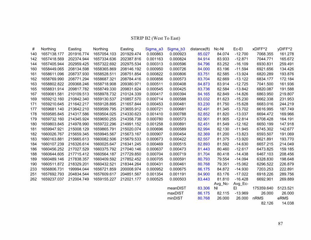
coordinates are given in Table 2.2. The columns in Table 2.2 are the strip name showing
the direction of the flight and the number of strip, mean distance between the actual
horizontal coordinates and LSIM derived coordinates from un-calibrated LIDAR data,
maximum distance, minimum distance, mean values for the difference between northing
Page 45
40
Figure 2.16 Lidar points around the control point 267
Table 2.2 Control point comparison in horizontal coordinates
Strip meanDIST maxDIST minDIST Avg_Nc-Nl Avg_Ec-El nRMS eRMS #c.ptsa1 81.1650 83.6017 71.5062 -75.9819 28.5059 76.0304 28.5784 13a2 82.2839 84.8512 79.8052 -76.6667 29.8573 76.6801 29.8928 25a3 84.2599 86.7470 79.8857 -70.5806 28.9670 78.5291 30.6131 21a4 85.4990 86.5733 82.3717 -79.5989 31.1909 79.6073 31.2287 5b1 84.0760 85.4474 81.6091 82.9946 -13.4152 83.0038 13.4491 13b2 83.3062 86.1751 80.7676 82.1148 -13.9690 82.1255 14.0378 26b3 82.8520 86.9376 78.9945 68.8829 -10.2560 81.3769 15.6811 26b4 80.9037 82.4256 79.1451 79.7094 -13.8242 79.7163 13.8552 9
Mean 83.0432 85.3449 79.2606 1.3592 8.3821 79.6337 22.1670 17.25 Strip meanDIST maxDIST minDIST Avg_Nc-Nl Avg_Ec-El nRMS eRMS #c.ptsa1 81.1650 83.6017 71.5062 -75.9819 28.5059 76.0304 28.5784 13a2 82.2839 84.8512 79.8052 -76.6667 29.8573 76.6801 29.8928 25a3 84.2599 86.7470 79.8857 -70.5806 28.9670 78.5291 30.6131 21a4 85.4990 86.5733 82.3717 -79.5989 31.1909 79.6073 31.2287 5
Mean 83.3020 85.4433 78.3922 -75.7070 29.6303 77.7117 30.0782 16.00 Strip meanDIST maxDIST minDIST Avg_Nc-Nl Avg_Ec-El nRMS eRMS #c.ptsb1 84.0760 85.4474 81.6091 82.9946 -13.4152 83.0038 13.4491 13b2 83.3062 86.1751 80.7676 82.1148 -13.9690 82.1255 14.0378 26b3 82.8520 86.9376 78.9945 68.8829 -10.2560 81.3769 15.6811 26b4 80.9037 82.4256 79.1451 79.7094 -13.8242 79.7163 13.8552 9
Mean 82.7845 85.2464 80.1291 78.4254 -12.8661 81.5556 14.2558 18.50
and easting coordinates and the RMS values for northing and easting values. The last
column shows the number of control points that fall in each strip. The strips can also be
seen in Figure 2.17 with the strip names and directions. Table 2.2 clearly shows a
boresight misalignment error existing in the data. All the units in Table 2.2 are in US
Page 46
41
Survey foot. The errors in the Easting range from 71.5 ft (21.79m) to 86.93 ft (26.50m).
In the next section an adjustment method is explained to remove this boresight
misalignment error. Appendix D shows all the comparisons for all strips.
Figure 2.17 LIDAR data strips showing the overlaps and the directions.
The directions of errors can be seen in Figure 2.18, which clearly shows the boresight
misalignment with some of the error magnitudes shown in feet.
Figure 2.18. Error directions due to Boresight misalignment
East to West
West to East
Page 47
42
2.4 ADJUSTING THE UNCALIBRATED DATA
LSIM analysis gives us the locations of the ground control points in the Lidar data. We
can use these values to adjust the uncalibrated Lidar data which has a major boresight
misalignment and elevation error. The research on methodologies of adjusting the data is
ongoing, and will be published as part of the doctoral research of the second author
(A.F.C.) of this report.
Page 48
43
CHAPTER 3
EDGE OF PAVEMENT EXTRACTION AND EVALUATION
Accurate terrain mapping is important for highway corridor planning and design,
environmental impact assessment, and infrastructure asset management. The management
of transportation infrastructure assets can be more efficient and cost-effective by using a
geographical information system (GIS) for defining georeferenced locations, storing
attribute data, and displaying data on maps. Collecting good-quality geographical
coordinate data by traditional ground-based manual methods may require a substantial
investment depending upon the size of the assets. In the case of natural or orchestrated
disasters, the assessment of damage and re-building can be costly and time-consuming if
the inventory and terrain model data are not easily available. Safe and efficient mobility
of goods and people requires periodic monitoring and maintenance of all transportation
infrastructure components within the right-of-way including the following: pavements,
bridges, tunnels, interchanges, roadside safety structures, and drainage structures. These
data collection activities require time- and labor-intensive efforts. In many parts of the
world, highway data are collected at highway speed using noncontact photography,
video, laser, acoustic, radar, and infrared sensors. These terrestrial noncontact
technologies may suffer limitations resulting from time of day, traffic congestion, and
proximity to urban locations. Additionally, traditional terrestrial ground surveys can be
quite hazardous, especially in the areas of maintenance work zones. Modern airborne and
Page 49
44
spaceborne remote-sensing technologies offer cost-effective terrain mapping, inventory,
and monitoring data collection [121].
Traditionally, high-altitude (about 3,000 m or 10,000 ft above ground) commercial aerial
photogrammetry (passive sensor) has been used to produce orthorectified photos and
digital elevation models for most transportation and landuse planning and engineering
studies. The new innovative airborne laser survey missions (active sensors) are flown at
about 500 m or 1,500 ft above ground level.
Several key components on airside and landside operations are similar in these airborne
technologies. Table 3.1 compares operating characteristics and data resolution of several
remote sensing technologies [121].
Table 3.1. Comparison of the new ‘high resolution’ spaceborne and airborne remote sensing technologies
Satellite/ Airborne Spatial
Resolution Spectral
Resolution
Temporal Resolution
days Footprint (km x km)
Landsat 7 15m 7 bands 16 185x185 IKONOS 1 m 3 bands 3.5-5 11x11
Quickbird2 0.61m 3 bands 1.5-4 16.5x16.5
ASTER VNIR:15m IR: 30-90 m 14 bands In Space
Shuttle Variable
Orbview3 1m 4 bands 3 8x8
SPOT5 2.5m Mid IR:20 m 4 bands 04-Jan 60x60
Aerial Photo Upto 0.15m Visible
band On Demand 2x2 at 3000m
Airborne Lidar Upto 0.15m NIR band On Demand Very
Dense*
IR = Infrared, NIR = Near Infrared, VNIR = Very Near Infrared * LIDAR measurement at 500 m above terrain level: about 1 m x 1 m on ground
Page 50
45
Transportation projects require detailed terrain and land cover maps for corridor
planning, environmental assessment and engineering design. The applications are so
diverse in their requirements that mapping has to be repeated at a number of different
scales, from 1:600 for design to 1:50,000 for corridor planning. In many cases, traditional
field survey methods have given way to photogrammetry, using either traditional
analytical stereo-plotters or modern soft-copy photogrammetry. Photogrammetry from
low-altitude photography (flown as low as 150 m) can produce elevation accuracy in the
range of 2 cm. This may be used, for example, to calculate the volume of material to be
stripped off a road surface. About half of all state and local photogrammetry work is
contracted to the private sector; hence these firms face the same pressures as do DOTs to
adopt the new technologies [122].
The LIDAR technology has few constraints typical to conventional topographic survey
methods. It can survey day and night, at altitudes between 300 and 900 m (1,000 to 3,000
ft) above ground, over any terrain, and through most vegetation and canopy. Most of the
highway application surveys are conducted at a height of 500 m (1,500 ft) above ground
level. A typical survey can collect data at a rate of up to 81 sq. km (20,000 acres) per day
[121].
For the last few years it has been shown in many research papers that automated feature
extraction from Lidar data is a very promising issue. However achieving the required
accuracies for design stages using the automated technologies is a challenging issue. But
the quality and the quantity of the Lidar data may provide a high accuracy 3D feature
extraction environment.
Page 51
46
Highway corridor mapping is an important task for most DOTs in the U.S. which is
mainly done for evaluation of the existing infrastructure. In this research, the edge of
pavements on the roads will be extracted from the Lidar data and the accuracy for the
extracted features along the project area will be compared with the ones derived from
aerial photogrammetry, and ground total station.
Before getting into the feature extraction the next section will introduce the highway
cross-section elements. The features that will be extracted this research are edge of
pavements.
3.1 Highway Cross-Section Elements
The principal elements of a highway cross-section consist of the travel lanes, shoulders,
and medians (for some multilane highways). Marginal elements include median and
roadside barriers, curbs, gutters, guard rails, sidewalks, and side slopes. These are typical
elements of cross sections of two-lane highways or multilane highways.
Shoulders
Travel lane widths usually vary from 10 ft to 12 ft. One of the elements of a section of a
highway cross-section are those designated as shoulders. The shoulder is contiguous
with the traveled lane and provides an area along the highway for vehicles to stop,
particularly during an emergency. Shoulders are also used to laterally support the
pavement structure. The shoulder width is known as either graded or usable, depending
on the section of the shoulder being considered. The graded shoulder width is the whole
Page 52
47
width of the shoulder measured from the edge of the traveled pavement to the intersection
of the shoulder slope and the plane of the side slope. The usable shoulder width is that
part of the graded shoulder that can be used to accommodate parked vehicles. The usable
shoulder width is the same as the graded width, when the side slope is equal to or flatters
than 4:1, as the shoulder break is usually rounded to a width between 4 ft and 6 ft,
thereby increasing the usable width.
When a vehicle stops on the shoulder, it is desirable for it to be at least 1 ft and preferably
2 ft from the edge of the pavement. Based on this, American Association of State
Highway and Transportation Officials (AASHTO) recommends that usable shoulder
widths of at least 10 ft and preferably 12 ft be used on highways having a large number of
trucks and on highways with high traffic volumes and high speeds. However, it may
always be feasible to provide this minimum width, particularly when the terrain is
difficult or when traffic volume is low. A minimum shoulder width of 2 ft may therefore
be used on the lowest type of highways, but 6 to 8 ft widths should preferably be used.
The width for usable shoulders within the median for divided arterials having two lanes
in each direction, however, may be reduced to 3 ft, since the drivers rarely use the median
shoulder for stopping on these roads. The usable median shoulder width for divided
arterials with three or more lanes in each direction should be at least 8 ft, since drivers in
difficulty on the lane next to the median often find it difficult to maneuver to the outside
shoulder.
Page 53
48
Medians
A median is the section of a divided highway that separates the lanes in opposing
directions. The width of a median is the distance between the edges of the inside lanes,
including the median shoulders. Medians can either be raised, flush, or depressed. Raised
medians are frequently used in urban arterial streets. Flush medians are commonly used
on urban arterials. They can also be used on freeways, but with a median barrier.
Depressed medians are generally used on freeways. Median widths vary from a minimum
of 2 ft to 80 ft or more. AASHTO recommends a minimum width of 10 ft for four-lane
urban freeways, which is adequate for two 4 ft shoulders, and a 2 ft median barrier. A
minimum of 22 ft, preferably 26 ft, is recommended for six or more lanes of freeway.
Median and Roadside Barriers
AASHTO defines a median barrier as a longitudinal system used to prevent an errant
vehicle from crossing the portion of a divided highway separating the traveled ways for
traffic in opposite directions.
Curbs and Gutters
Curbs are raised structures made of either Portland cement concrete or bituminous
concrete (rolled asphalt curbs) that are used mainly on urban highways to delineate
pavement edges and pedestrian walkways. Gutters or drainage ditches are usually located
on the pavement side of a curb to provide the principal drainage facility for the highway.
Guard Rails
Guard rails are longitudinal barriers placed on the outside of sharp curves and sections
with high fills. Their main function is to prevent vehicles from leaving the roadbed.
Sidewalks
Page 54
49
Sidewalks are usually provided on roads in urban areas, but very seldom are they
provided in rural areas.
Cross Slopes
Pavements on straight sections of two-lane and multilane highways without medians are
sloped from the middle downward to both sides of the highway. The cross slopes on
divided highways are provided by either crowning the pavement in each direction, or by
sloping the entire pavement in one direction.
Side Slopes
Side slopes are provided on embankments and fills to provide stability for earthworks.
They also serve as a safety feature by providing a recovery area for out-of-control
vehicles
Right of Way
The right of way is the total land area acquired for the construction of the highway [116].
3.2 Feature Extraction
For the last few years it has been shown in many research papers that automated feature
extraction from Lidar data is a very promising issue. However achieving the required
accuracies for design stages using the automated technologies is a challenging issue. But
the quality and the quantity of the Lidar data may provide a high accuracy 3D feature
extraction environment.
Both intensity and height information will be used for the extraction of road surfaces and
delineation of the edge of pavements in the project area. First of all non-terrain objects
such as vegetation, buildings, cars, etc. should be identified. To investigate the
Page 55
50
separability of these objects a clustering analysis will be performed. And then fusing the
elevation information with the intensity will help extraction of road surfaces from the
data. Using edge operators edge of pavements will be delineated and applying Hough
transform will give us the coordinates of points lying on the edge of pavements.
To see the intensity range for the features inside the data, clustering is performed using
MultiSpec data analysis software (ISODATA algorithm, number of classes 8,
convergence threshold 98%). A portion of the data (Figure 3.1) is used for this analysis
for testing purposes. After several attempts 8 clusters found to represent the data better.
Figure 3.1 Intensity Image used for clustering
Page 56
51
Figure 3.2 Clustering Results
Figure 3.3 Closer look at the clustered image
Page 57
52
Looking at figures 3.2 and 3.3 we can see that cluster #1 represents mainly buildings,
cluster #2 represents the grass, cluster #3 represents mainly vegetation but it also has
buildings and roads, cluster #4, 5, and 6 represents mainly roads and parking lots but it
also has building and vegetation, cluster #7 represents roads and buildings and cluster #8
represents water and buildings. This analysis shows us that by applying only some
threshold values to the intensity image it is impossible to extract any object from the Lida
data. But fusing the height values with the intensity and using the first-last return analysis
for the Lidar data can be the solution for road surface extraction problem.
To use the elevation information for the separation of the roads a bare earth Digital
Terrain Model of the area should be determined, which means the removal of the non-
terrain objects from the data.
An inherent source of information for the segmentation of Lidar data is the analysis of
height texture defined by local variations of height. The following results show the
application of the standard deviation filter to the intensity and height data. Energy,
Entropy, Contrast statistics derived from co-occurrence matrices will also be derived to
be used for clustering and a possible multi-spectral edge detection process.
To apply the standard deviation filter to the intensity and height image a block of the data
which has highway, streets, buildings, and vegetation is cropped. Figure 3.4 shows the
intensity image for this area. Figure 3.5 shows the result of the application of the standard
Page 58
53
Figure 3.4 Intensity image for standard deviation filter
deviation filter. When Standard Deviation Filter is applied to the intensity image each
output pixel contains the standard deviation of the 3-by-3 neighborhood around the
corresponding pixel in the input image.
Page 59
54
Figure 3.5 Standard deviation filter applied intensity image
Another texture measure, Entropy filter is also applied to the intensity image and the
result is presented in Figure 3.6. Looking at the results of this filter for the intensity
image gives us some idea about the edge of pavements, especially the standard deviation
filter but this is not enough. We decided to apply the standard deviation filter to the
height image (Figure 3.7). Height image itself is a very good texture measure to identify
some objects in the scene such as high buildings and vegetation.
Page 60
55
Figure 3.6 Entropy filter applied intensity image
Figure 3.7 Height image
Page 61
56
Figure 3.8 Standard deviation filter applied height image
Looking at Figure 3.8 we can easily identify the non-terrain objects (buildings, trees,
cars. Applying a 90% threshold value to this image gives us a binary image showing the
non-terrain objects (Figure 3.9). To delineate the pixels defining the non-terrain objects
some morphological operations are performed on the threshold applied filtered height
image. A closing operation is followed by an opening operation and then filling up the
holes gives us the non-terrain objects which can be seen in Figure 3.10. We can clearly
see the cars, buildings and trees in this image. To obtain the bare earth DTM we take a
compliment of this image which gives the roads, surrounding grass and earth pixels
(Figure 3.11).
Page 62
57
Figure 3.9 Threshold application
Figure 3.10 Non-terrain objects
Page 63
58
Figure 3.11 Bare Earth pixels
By removing the non-terrain pixels from the intensity image we get output which has
only the bare earth pixels in Figure 3.12. Now we can cluster this image to separate the
road surfaces from the Lidar data as in Figures 3.13 and 3.14. After performing opening
and closing morphological operations on the separated road surfaces (Figure 3.15) we can
clearly see the road surfaces which include the parking lots in Figure 3.16. And finally,
applying an edge detection algorithm (Canny Edge detection method) to the final image
gives us the edge of pavements for the area.
Page 64
59
Figure 3.12 Intensity image without non-terrain objects
Figure 3.13 Clustered image showing road surfaces
Page 65
60
Figure 3.14 Separated road surfaces
Figure 3.15 Opening and closing operation on road surfaces
Page 66
61
Figure 3.16 Road surfaces over intensity image
Figure 3.17 Application of Canny edge detection over Road surfaces
Page 67
62
When we look at the figures 3.16 and 3.17 we see that the method does not give a very
good result for edge of pavements. The trees block some of the road surfaces, so the last
return data for the surfaces should be included where the trees are removed. The raildroad
inside the image also included as a road feature and it has to be removed, too. The surface
under the vehicles should be interpolated. The median on the highway should be
identified and the highway edge of pavements should be clearly delineated. The feature
extraction and evaluation is not finished yet but the research is continuing. The following
steps are to be done;
• Deriving other texture measures for clustering and multi-spectral edge detection
• Extraction of edge of pavements using Hough Transform
• Comparison of the results with the data collected for INDOT for the same project
area.
Page 68
63
CHAPTER 4
FIELD TRIP TO ODOT
A visit to ODOT (Ohio Department of Transportation) is planned and done on Dec.16,
2005 to discuss our findings in the project and to see how they compare to their
experience. It was a very helpful trip. This section summarizes the observations during
that trip.
After investigating their options ODOT bought a Lidar system to operate themselves for
faster processing of large linear jobs. Selection of a Lidar system depends on criteria such
as functionality, cost, upgrade potential, maintenance program, and other options. The
department preferred a fixed wing aircraft (Cessna Grand Caravan) since it is better than
a helicopter when the vibration, maintenance costs and flying time is considered although
the flying height for helicopters can be as low as 80m when compared to 300m for fixed
wing (Figure 4.1).
Page 69
64
Figure 4.1 Cessna Grand Caravan Lidar instrumentation
But then the swath width for the flight decreases due to the lower heights. The other
items that are considered for the selection of the airplane were cabin floor area, fuel
duration, cost, safety record, operating characteristics and payload capacity. After
selection of the aircraft the interior design should be made to put all the instruments.
ODOT has Optech ALTM 30/70 Lidar equipment.
Besides the systems onboard the aircraft there has to be data storage systems which
should store terabytes of data. There has to be an archival, and an expansion plan for the
units. Multiple hard drives, lots of memory and dual processors are some of the
requirements for the workstations.
The software packages that are used for the data management purposes are:
• Geomedia – Plan mapping extents
• ALTM NAV – Plan and conduct flights
• POSPAC – GPS/INS solution
• Realm – Point cloud generation
• GeoCue – Review coverage, create working segments, LiDAR ortho’s, manage
workflow
• Microstation V8 – CAD software
Page 70
65
• TerraScan – classification, thinning, smoothing
• TerraMatch – Rectify flight lines if necessary
• QT Modeler – 3D visualization
• TerraPhoto – AT and orthophoto production
• ISAT – Auto AT
• OrthoPro – Orthophoto production
• GeoPac – Microstation Design software
Selection of the software should be done according to the application/products,
goal/design quality, and approach/Lidar for the surface and photogrammetry for the
planimetrics.
One of the softwares is GeoCue which can use other softwares for several purposes.
GeoCue is applicable to just about any production or task management scenario that
follows the paradigm of input of data, dividing the data into production “segments” and
then processing the data into products (http://www.niirs10.com/Products/geocue.htm).
QT Modeler is the software used for visualization purposes which is now being marketed
by Applied Imagery (www.appliedimagery.com). The story of Applied Imagery begins at
the Johns Hopkins University's Applied Physics Lab (APL).
Another visualization software is PointVue LE. PointVue LE is a 3-D LIDAR
visualization tool which can be used to visualize LIDAR data in ASPRS LAS Version 1.1
format (http://www.niirs10.com/Products/pointvue.htm).
The data extraction software form the Lidar equipment is Realm Survey.
Page 71
66
POSPac software is used for fully exploit data collected with the company's Position and
Orientation System (POS), Digital Sensor System (DSS), as well as LIDAR and camera
systems (http://www.applanix.com/products/pospac_airborne_index.php).
For processing laser-scanning points Terrascan is used. Processing includes error
calibration, point classification, removal of unnecessary points, profile extraction and
digitizing features by snapping onto laser points
(http://www.terrasolid.fi/ENG/Tuote_kuvaukset/TScan.htm).
The main output from their system is a Digital Terrain Model of the project area. By only
producing this data the system paid of itself in one year.
Some of the conclusions from ODOT projects are:
• Vertical accuracy needed for planning stages is ± 1.0 ft and ±0.1 ft for design
stages. The planimetric accuracy that is asked is 0.2-0.3ft.
• LiDAR can be used with existing softcopy photogrammetry
• LiDAR can meet planning level mapping needs with little processing
• LiDAR can meet design level mapping if appropriate control and processing is
performed
• Survey control must be obtained as accurately as possible
• High point density is essential for design level mapping
• Photogrammetry is used for small jobs; Lidar is used for DTM generation on
moderate and large jobs, special projects [123].
Page 72
67
The project area is shown in Figures 4.2, 4.3 which are produced using QT Modeler
software.
Whole project area Another oblique view the project area
Figure 4.2 Scenes from the project area produced using QT Modeler with elevation values
Page 73
68
Figure 4.3 Scenes from the project area produced using QT Modeler with intensity values
Page 74
69
CHAPTER 5
CONCLUSIONS
With properly designed LIDAR control, assessment of 3D as built is attainable at the
over-all average horizontal (planimetric) error of 0.324 ft (9.9 cm); more specifically with
a 0.284 ft (8.7 cm) RMS error in Northing, and a 0.255 ft (7.8 cm) RMS error in Easting.
The over-all average vertical (height) error was 0.003 ft (0.09 c,m). The RMS error in
height was 0.108 ft (3.29cm).
Lidar recognizable control (2m x 2m chevrons) was spaced at approximately 200m
parallel to the axis of the project corridor, at a 60m spacing sideways. The corridor
project was about 6 km long.
Least Squares Image matching software was developed. The internal accuracy proved to
be 0.027 ft (8mm).
The strip width was approximately 111m and overlap between the Lidar strips changes
from 55 to 90m sideways. Each flight line was flown twice in opposite directions
showing 55 % overlap in two strips and 75 % in other two.
The overall conclusion about the usage of Lidar aerial surveys for corridor mapping
projects is that this technique is an efficient, cost cutting alternative to classical terrestrial
and aerial survey techniques. However, at this point of the research it is felt that the
design of the LiDAR control plays a critical role to the success of the deployment of
aerial LiDAR surveys. Augmentation of ground-based LiDAR and classical surveys
Page 75
70
proves to be necessary because of shielding of the airborne laser signals (e.g.
underpasses).
Comparison of the Lidar based model against the photogrammetric model obtained from
low flying aerial photography (helicopter) should be made once data of the latter model
become available.
Page 76
71
CHAPTER 6
REFERENCES [100] Axelsson, P., 1999. Processing of laser scanner data—algorithms and applications,
ISPRS Journal of Photogrammetry & Remote Sensing, 54:138–147.
[101] Csanyi N, Toth C. K., Grejner-Brzezinska D., Ray J., Improvement Of Lidar Data
Accuracy Using Lidar Specific Ground Targets, ASPRS 2005 Annual Conference
Baltimore, Maryland, March 7-11, 2005
[102] Baltsavias, E.P., 1999. Airborne laser scanning: basic relations and formulas,
ISPRS Journal of Photogrammetry & Remote Sensing, 54:199-204.
[103] Wehr, A., and U. Lohr, 1999. Airborne laser scanning—an introduction and
overview, ISPRS Journal of Photogrammetry & Remote Sensing, 54: 68–82.
[104] Morin, K., and El-Sheimy, N. 2002. Post-mission Adjustment Methods of Airborne
Laser Scanning Data, FIG XXII International Congress, Washington, D.C. USA.
[105] Kilian J., Haala, N., Englich, M. (1996). Capture and Evaluation of Airborne Laser
Scanner Data. International Archives of Photogrammetry and Remote Sensing, Vol.
XXXI, Part B3, pp. 383-388.
[106] Burman, H. (2000). Adjustment of Laser Scanner Data for Correction of
Orientation Errors. International Archives of Photogrammetry and Remote Sensing, Vol.
XXXIII, Part B3, pp. 125-132.
[107] Burman, H. (2002). Laser Strip Adjustment for Data Calibration and Verification.
In ISPRS Commission III, Symposium 2002 September 9 - 13, 2002, Graz, Austria,
pages A-067 ff (6 pages), 2002.
Page 77
72
[108] Crombaghs, M. J.E.,R. Brügelmann, E.J. de Min, 2000. On the adjustment of
overlapping strips of laseraltimeter height data. International Archives of
Photogrammetry and Remote Sensing, Vol. XXXIII, Part B3/1, pp. 224-231.
[109] Maas, H-G, 2001. On the Use of Pulse Reflectance Data for Laserscanner Strip
Adjustment. IAPRS, Vol XXXIV Annapolis, 2001.
[110] Filin, S. (2001). Recovery of Systematic Biasaes in Laser Altimeters Using Natural
Surfaces. International Archives of Photogrammetry and Remote Sensing, Vol. XXXIV,
Part 3/W4, pp. 85-91.
[111] Toth C., Csanyi N. and Grejner-Brzezinska D. 2002. Automating the Calibration of
Airborne Multisensor Imaging Systems, Proc. ACSM-ASPRS Annual Conference,
Washington, DC, April 19-26, CDROM.
[112] Katzenbeisser, R. 2004. Calibration and Data Validation of A Lidar Fiber Scanner.
ASPRS Annual Conference May 24 to 27, 2004 Denver CO.
[113] Bethel, J. LEAST SQUARES IMAGE MATCHING for CE604.
[115] Uddin, W., 2002, Evaluation of airborne Lidar Digital Terrain Mapping for
Highway Corridor Planning and Design. Pecora 15/Land Satellite Information IV/ISPRS
Commission I/FIEOS 2002 Conference Proceedings.
[116] Garber, N. J., Hoel, L.A., 1997. Traffic and Highway Engineering. PWS Publishing
Company.
[118] http://www.airbornelasermapping.com
Page 78
73
[119] Hodgson, M.E., Bresnahan P.,2004. Accuracy of Airborne Lidar-Derived
Elevation:Empirical Assessment and Error Budget, Photogrammetric Engineering &
Remote Sensing Vol. 70, No. 3, March 2004, pp. 331–339.
[120] Flood M.,Satalich J., LiDAR 101,
http://pobonline.com/CDA/ArticleInformation/Article/0,9169,23513,00.html, accessed
October 2005.
[121] Uddin W., 2002, Evaluation of Airborne Lidar Digital Terrain Mapping For
Highway Corridor Planning And Design, Pecora 15/Land Satellite Information IV/ISPRS
Commission I/FIEOS 2002 Conference Proceedings
[122] National Consortia on Remote Sensing in Trnasportation (NCRST),REMOTE
SENSING AND SPATIAL NFORMATION TECHNOLOGIES IN
TRANSPORTATION, Synthesis Report 2001
[123] Joe Tack, John A. Ray. ODOT Office of Aerial Engineering Presentation. ODOT’s
Experience with LiDAR for Design and Planning Level Mapping, ASPRS 2005.
Page 79
74
APPENDIX A
Control Comparison Unadjusted
Number Easting Northing Known Z Laser Z Dz --------------------------------------------------------------------- 130 199378.650 1655755.703 744.780 744.020 -0.760 132 199818.110 1656139.531 749.530 748.940 -0.590 133 200093.884 1655807.529 752.340 751.430 -0.910 134 200165.720 1656508.201 753.700 753.010 -0.690 135 200408.865 1656281.570 779.820 779.210 -0.610 136 200597.350 1656957.308 756.440 755.780 -0.660 137 200927.969 1656627.696 757.740 757.120 -0.620 138 201297.810 1656870.779 775.950 775.290 -0.660 139 201173.775 1657308.593 771.050 770.460 -0.590 140 201916.774 1657138.177 772.950 772.420 -0.530 142 202374.944 1657418.569 777.879 777.170 -0.709 143 202651.589 1657810.773 771.001 770.370 -0.631 144 202959.425 1657405.944 777.017 776.210 -0.807 145 203365.627 1657822.824 777.155 776.560 -0.595 146 203626.829 1657284.615 780.807 780.160 -0.647 147 204088.429 1657593.231 782.757 782.030 -0.727 148 204306.485 1657128.402 783.227 782.630 -0.597 149 204953.999 1657124.773 787.410 786.630 -0.780 150 204818.667 1657388.081 788.001 787.210 -0.791 151 205638.790 1656992.112 790.833 790.050 -0.783 152 205638.167 1657427.201 787.235 786.590 -0.645 153 206194.353 1657306.696 777.047 776.230 -0.817 154 206221.467 1657459.828 776.203 775.390 -0.813 155 206795.422 1657610.299 789.357 788.650 -0.707 156 206842.996 1657780.449 791.214 790.490 -0.724 157 207457.213 1657954.471 795.351 794.700 -0.651 158 207495.574 1658117.305 795.891 795.370 -0.521 159 208086.918 1658279.805 798.760 798.020 -0.740 160 208134.598 1658449.065 799.458 798.810 -0.648 161 208737.930 1658611.096 801.479 800.880 -0.599 162 208771.294 1658769.990 804.370 803.610 -0.760 163 209368.246 1658802.822 804.183 803.410 -0.773 164 209415.091 1658967.989 808.337 807.800 -0.537 165 209817.782 1658831.914 804.258 803.490 -0.768 166 210208.320 1658684.342 812.967 812.150 -0.817 167 210109.513 1659061.581 808.134 807.420 -0.714 168 210953.873 1658714.346 833.407 832.750 -0.657 169 210842.340 1659212.160 821.699 821.020 -0.679 170 211668.528 1658739.419 813.631 813.020 -0.611
Page 80
75
171 211642.217 1659210.645 817.384 816.760 -0.624 172 212307.276 1658936.437 823.325 822.670 -0.655 173 212362.023 1659111.245 820.578 819.960 -0.618 174 212973.544 1659144.455 833.684 833.020 -0.664 175 213015.607 1659304.426 835.255 834.410 -0.845 176 213643.317 1659229.457 828.313 827.680 -0.633 177 213642.210 1659681.140 828.950 828.200 -0.750 178 214317.586 1659585.845 843.452 842.670 -0.782 179 214345.924 1659732.160 842.923 842.340 -0.583 180 214978.990 1659803.845 840.876 840.200 -0.676 181 215008.129 1659947.921 841.440 840.860 -0.580 182 215659.345 1660026.767 852.686 852.170 -0.516 183 215665.613 1660163.881 853.500 852.980 -0.520 184 216326.614 1660107.239 839.700 839.030 -0.670 185 216322.186 1660586.939 846.319 845.650 -0.669 186 217027.529 1660456.252 854.760 854.000 -0.760 187 217022.241 1660596.252 857.720 857.120 -0.600 188 217715.412 1660644.605 852.060 851.300 -0.760 189 217838.357 1660489.146 850.980 850.330 -0.650 190 218329.201 1660511.872 867.100 866.450 -0.650 191 218526.100 1660106.246 853.460 852.750 -0.710 192 218826.737 1660258.473 881.450 880.760 -0.690 193 219118.197 1659821.622 881.860 881.330 -0.530 195 219306.505 1660091.852 857.510 856.820 -0.690 232 199420.595 1656032.097 742.080 741.320 -0.760 233 199994.044 1656806.731 745.870 745.300 -0.570 236 200302.321 1657122.825 753.530 752.860 -0.670 237 200612.192 1657401.508 754.000 752.770 -1.230 238 201215.212 1656296.602 761.610 761.020 -0.590 240 201674.727 1656553.373 766.760 766.240 -0.520 242 202353.978 1656826.049 772.979 772.220 -0.759 244 202834.360 1657146.020 775.546 774.850 -0.696 246 203288.890 1657034.452 779.447 778.780 -0.667 247 203770.077 1658054.986 777.655 777.100 -0.555 248 203957.593 1656912.639 782.926 782.210 -0.716 249 204327.256 1657944.902 781.203 780.560 -0.643 251 204834.544 1657692.793 783.819 783.090 -0.729 253 205465.056 1657688.295 787.212 786.390 -0.822 254 205688.559 1657699.373 787.459 786.800 -0.659 256 209949.694 1658121.393 800.264 799.570 -0.694 257 210487.958 1658144.452 805.273 804.420 -0.853 259 211050.863 1658167.265 838.857 838.090 -0.767 262 212004.749 1659237.037 816.873 816.230 -0.643 263 211984.705 1659578.542 817.768 817.200 -0.568 264 213644.530 1658759.639 832.929 832.080 -0.849 265 213866.100 1658737.988 833.964 833.070 -0.894
Page 81
76
266 213798.339 1660103.339 831.636 830.960 -0.676 267 216269.311 1659858.646 835.760 835.130 -0.630 269 216553.703 1659731.064 837.665 837.070 -0.595 Average dz -0.687 Average magnitude 0.687 Root mean square 0.695 Std deviation 0.109
Page 82
77
APPENDIX B
Control Comparison Adjusted
Number Easting Northing Known Z Laser Z Dz --------------------------------------------------------------------- 130 199378.650 1655755.703 744.780 744.710 -0.070 132 199818.110 1656139.531 749.530 749.630 +0.100 133 200093.884 1655807.529 752.340 752.120 -0.220 134 200165.720 1656508.201 753.700 753.700 +0.000 135 200408.865 1656281.570 779.820 779.900 +0.080 136 200597.350 1656957.308 756.440 756.470 +0.030 137 200927.969 1656627.696 757.740 757.810 +0.070 138 201297.810 1656870.779 775.950 775.980 +0.030 139 201173.775 1657308.593 771.050 771.150 +0.100 140 201916.774 1657138.177 772.950 773.110 +0.160 142 202374.944 1657418.569 777.879 777.860 -0.019 143 202651.589 1657810.773 771.001 771.060 +0.059 144 202959.425 1657405.944 777.017 776.900 -0.117 145 203365.627 1657822.824 777.155 777.250 +0.095 146 203626.829 1657284.615 780.807 780.850 +0.043 147 204088.429 1657593.231 782.757 782.720 -0.037 148 204306.485 1657128.402 783.227 783.320 +0.093 149 204953.999 1657124.773 787.410 787.320 -0.090 150 204818.667 1657388.081 788.001 787.900 -0.101 151 205638.790 1656992.112 790.833 790.740 -0.093 152 205638.167 1657427.201 787.235 787.280 +0.045 153 206194.353 1657306.696 777.047 776.920 -0.127 154 206221.467 1657459.828 776.203 776.080 -0.123 155 206795.422 1657610.299 789.357 789.340 -0.017 156 206842.996 1657780.449 791.214 791.180 -0.034 157 207457.213 1657954.471 795.351 795.390 +0.039 158 207495.574 1658117.305 795.891 796.060 +0.169 159 208086.918 1658279.805 798.760 798.710 -0.050 160 208134.598 1658449.065 799.458 799.500 +0.042 161 208737.930 1658611.096 801.479 801.570 +0.091 162 208771.294 1658769.990 804.370 804.300 -0.070 163 209368.246 1658802.822 804.183 804.100 -0.083 164 209415.091 1658967.989 808.337 808.490 +0.153 165 209817.782 1658831.914 804.258 804.180 -0.078 166 210208.320 1658684.342 812.967 812.840 -0.127 167 210109.513 1659061.581 808.134 808.110 -0.024 168 210953.873 1658714.346 833.407 833.440 +0.033 169 210842.340 1659212.160 821.699 821.710 +0.011 170 211668.528 1658739.419 813.631 813.710 +0.079 171 211642.217 1659210.645 817.384 817.450 +0.066
Page 83
78
172 212307.276 1658936.437 823.325 823.360 +0.035 173 212362.023 1659111.245 820.578 820.650 +0.072 174 212973.544 1659144.455 833.684 833.710 +0.026 175 213015.607 1659304.426 835.255 835.100 -0.155 176 213643.317 1659229.457 828.313 828.370 +0.057 177 213642.210 1659681.140 828.950 828.890 -0.060 178 214317.586 1659585.845 843.452 843.360 -0.092 179 214345.924 1659732.160 842.923 843.030 +0.107 180 214978.990 1659803.845 840.876 840.890 +0.014 181 215008.129 1659947.921 841.440 841.550 +0.110 182 215659.345 1660026.767 852.686 852.860 +0.174 183 215665.613 1660163.881 853.500 853.670 +0.170 184 216326.614 1660107.239 839.700 839.720 +0.020 185 216322.186 1660586.939 846.319 846.340 +0.021 186 217027.529 1660456.252 854.760 854.690 -0.070 187 217022.241 1660596.252 857.720 857.810 +0.090 188 217715.412 1660644.605 852.060 851.990 -0.070 189 217838.357 1660489.146 850.980 851.020 +0.040 190 218329.201 1660511.872 867.100 867.140 +0.040 191 218526.100 1660106.246 853.460 853.440 -0.020 192 218826.737 1660258.473 881.450 881.450 +0.000 193 219118.197 1659821.622 881.860 882.020 +0.160 195 219306.505 1660091.852 857.510 857.510 +0.000 232 199420.595 1656032.097 742.080 742.010 -0.070 233 199994.044 1656806.731 745.870 745.990 +0.120 236 200302.321 1657122.825 753.530 753.550 +0.020 237 200612.192 1657401.508 754.000 753.460 -0.540 238 201215.212 1656296.602 761.610 761.710 +0.100 240 201674.727 1656553.373 766.760 766.930 +0.170 242 202353.978 1656826.049 772.979 772.910 -0.069 244 202834.360 1657146.020 775.546 775.540 -0.006 246 203288.890 1657034.452 779.447 779.470 +0.023 247 203770.077 1658054.986 777.655 777.790 +0.135 248 203957.593 1656912.639 782.926 782.900 -0.026 249 204327.256 1657944.902 781.203 781.250 +0.047 251 204834.544 1657692.793 783.819 783.780 -0.039 253 205465.056 1657688.295 787.212 787.080 -0.132 254 205688.559 1657699.373 787.459 787.490 +0.031 256 209949.694 1658121.393 800.264 800.260 -0.004 257 210487.958 1658144.452 805.273 805.110 -0.163 259 211050.863 1658167.265 838.857 838.780 -0.077 262 212004.749 1659237.037 816.873 816.920 +0.047 263 211984.705 1659578.542 817.768 817.890 +0.122 264 213644.530 1658759.639 832.929 832.770 -0.159 265 213866.100 1658737.988 833.964 833.760 -0.204 266 213798.339 1660103.339 831.636 831.650 +0.014
Page 84
79
267 216269.311 1659858.646 835.760 835.820 +0.060 269 216553.703 1659731.064 837.665 837.760 +0.095 Average dz +0.003 Average magnitude 0.081 Root mean square 0.108 Std deviation 0.109
Page 85
80
APPENDIX C
ELEVATION COMPARISON WITH CALIBRATED DATA
GCP # Northing Easting Elevation Northing Easting Avg. elev CNT
∆ Elevation
137 1656627.696 200927.969 757.740 1656627.482 200927.989 757.285 4 0.455138 1656870.779 201297.810 775.950 1656870.809 201297.800 775.356 4 0.594139 1657308.593 201173.775 771.050 1657308.461 201173.226 770.464 2 0.586140 1657138.177 201916.774 772.950 1657138.061 201916.919 772.587 4 0.363142 1657418.569 202374.944 777.879 1657418.480 202374.848 777.400 17 0.479143 1657810.773 202651.589 771.001 1657810.858 202651.688 770.458 5 0.543144 1657405.944 202959.425 777.017 1657405.530 202959.035 776.407 3 0.610145 1657822.824 203365.627 777.155 1657822.711 203365.621 776.682 3 0.473148 1657128.402 204306.485 783.227 1657128.295 204306.263 782.649 3 0.578149 1657124.773 204953.999 787.410 1657124.605 204954.048 786.741 3 0.669150 1657388.081 204818.667 788.001 1657387.870 204818.628 787.356 4 0.645151 1656992.112 205638.790 790.833 1656992.285 205638.337 790.022 1 0.811152 1657427.201 205638.167 787.235 1657427.297 205638.158 786.764 28 0.471153 1657306.696 206194.353 777.047 1657306.860 206194.311 776.563 3 0.484154 1657459.828 206221.467 776.203 1657460.018 206221.306 775.527 6 0.676155 1657610.299 206795.422 789.357 1657609.948 206795.798 788.690 2 0.667156 1657780.449 206842.996 791.214 1657780.887 206843.094 790.694 3 0.520157 1657954.471 207457.213 795.351 1657954.445 207456.980 794.785 4 0.566158 1658117.305 207495.574 795.891 1658117.540 207495.295 795.391 2 0.500159 1658279.805 208086.918 798.760 1658279.605 208086.758 798.132 7 0.628160 1658449.065 208134.598 799.458 1658449.013 208134.829 799.072 4 0.386161 1658611.096 208737.930 801.479 1658611.290 208738.031 800.969 3 0.510162 1658769.990 208771.294 804.370 1658770.060 208771.370 803.861 9 0.509163 1658802.822 209368.246 804.183 1658802.440 209367.913 803.506 2 0.677164 1658967.989 209415.091 808.337 1658967.526 209415.242 807.721 2 0.616165 1658831.914 209817.782 804.258 1658831.678 209817.836 803.636 3 0.621166 1658684.342 210208.320 812.967 1658684.363 210208.180 812.250 3 0.717167 1659061.581 210109.513 808.134 1659061.072 210109.801 807.630 8 0.504168 1658714.346 210953.873 833.407 1658714.283 210954.312 832.935 2 0.472169 1659212.160 210842.340 821.699 1659212.075 210842.299 821.199 7 0.500170 1658739.419 211668.528 813.631 1658738.837 211668.927 813.095 3 0.536171 1659210.645 211642.217 817.384 1659210.065 211642.151 816.819 3 0.565172 1658936.437 212307.276 823.325 1658935.889 212307.511 822.788 5 0.537173 1659111.245 212362.023 820.578 1659110.398 212362.579 820.113 4 0.465174 1659144.455 212973.544 833.684 1659144.155 212973.655 833.112 3 0.572175 1659304.426 213015.607 835.255 1659304.103 213015.877 834.672 18 0.583176 1659229.457 213643.317 828.313 1659229.148 213643.496 827.696 2 0.617177 1659681.140 213642.210 828.950 1659681.070 213642.441 828.337 4 0.613178 1659585.845 214317.586 843.452 1659585.762 214317.555 842.871 19 0.581179 1659732.160 214345.924 842.923 1659731.797 214346.052 842.514 3 0.409180 1659803.845 214978.990 840.876 1659803.859 214978.925 840.453 3 0.423181 1659947.921 215008.129 841.440 1659947.614 215008.267 840.987 3 0.453182 1660026.767 215659.345 852.686 1660026.575 215659.807 852.193 3 0.492183 1660163.881 215665.613 853.500 1660163.994 215665.546 853.110 6 0.390
Page 86
81
184 1660107.239 216326.614 839.700 1660107.035 216327.437 839.171 3 0.529185 1660586.939 216322.186 846.319 1660586.890 216321.958 845.788 5 0.531186 1660456.252 217027.529 854.760 1660456.053 217027.542 854.300 8 0.460187 1660596.252 217022.241 857.720 1660596.313 217022.468 857.316 3 0.404188 1660644.605 217715.412 852.060 1660644.209 217715.746 851.554 12 0.506189 1660489.146 217838.357 850.980 1660489.176 217838.413 850.408 3 0.572190 1660511.872 218329.201 867.100 1660511.485 218329.401 866.590 4 0.510191 1660106.246 218526.100 853.460 1660106.204 218526.414 852.911 5 0.549192 1660258.473 218826.737 881.450 1660257.821 218826.584 880.824 3 0.626195 1660091.852 219306.505 857.510 1660091.382 219306.332 856.975 4 0.535233 1656806.731 199994.044 745.870 1656806.618 199994.299 745.397 5 0.473240 1656553.373 201674.727 766.760 1656553.243 201674.957 766.313 5 0.447242 1656826.049 202353.978 772.979 1656825.918 202353.783 772.454 4 0.525244 1657146.020 202834.360 775.546 1657145.954 202834.726 775.049 19 0.497246 1657034.452 203288.890 779.447 1657033.940 203289.315 778.927 3 0.520249 1657944.902 204327.256 781.203 1657944.925 204327.271 780.654 3 0.549251 1657692.793 204834.544 783.819 1657692.637 204834.420 783.166 3 0.653253 1657688.295 205465.056 787.212 1657688.251 205465.218 786.678 7 0.534254 1657699.373 205688.559 787.459 1657699.450 205688.257 786.844 3 0.615262 1659237.037 212004.749 816.873 1659236.809 212004.740 816.390 2 0.484263 1659578.542 211984.705 817.768 1659578.317 211984.435 817.271 4 0.498267 1659858.646 216269.311 835.760 1659858.435 216269.499 835.209 4 0.551269 1659731.064 216553.703 837.665 1659731.007 216553.609 837.216 5 0.449
Average Elevation Diff.= 0.539
Page 87
82
APPENDIX D
CONTROL POINT COMPARISON FOR EACH STRIP
STRIP A1 (East To West)
# Northing Easting Northing Easting Sigma_a3 Sigma_b3 distance(ft) Nc-Nl Ec-El xDIFF^2 yDIFF^2 139 1657308.593 201173.775 1657386.869 201144.834 0.000675 0.000554 83.455 -78.276 28.941 6127.084 837.584 142 1657418.569 202374.944 1657496.154 202347.151 0.000761 0.000653 82.413 -77.585 27.793 6019.380 772.465 143 1657810.773 202651.589 1657878.312 202628.102 0.000623 0.000555 71.506 -67.539 23.486 4561.521 551.613 145 1657822.824 203365.627 1657899.452 203334.106 0.000700 0.000735 82.857 -76.628 31.521 5871.776 993.551 249 1657944.902 204327.256 1658022.117 204297.370 0.000500 0.000697 82.797 -77.215 29.886 5962.153 893.171 162 1658769.990 208771.294 1658847.604 208740.824 0.000799 0.000514 83.381 -77.614 30.470 6023.999 928.422 164 1658967.989 209415.091 1659046.576 209386.572 0.000543 0.000386 83.602 -78.587 28.520 6175.878 813.366 167 1659061.581 210109.513 1659138.851 210081.905 0.000382 0.000310 82.053 -77.270 27.607 5970.611 762.165 169 1659212.160 210842.340 1659288.758 210812.464 0.000571 0.000519 82.219 -76.598 29.876 5867.298 892.601 263 1659578.542 211984.705 1659654.079 211953.931 0.000324 0.000359 81.565 -75.537 30.773 5705.896 947.005 185 1660586.939 216322.186 1660661.674 216294.760 0.000394 0.000386 79.608 -74.735 27.425 5585.352 752.154 187 1660596.252 217022.241 1660671.204 216995.523 0.000491 0.000490 79.572 -74.952 26.719 5617.763 713.892 188 1660644.605 217715.412 1660719.834 217687.853 0.000513 0.000530 80.117 -75.229 27.558 5659.350 759.457
meanDIST 81.165Avg
_Nc-Nl Avg_ Ec-El 75148.060 10617.446
maxDIST 83.602 -75.982 28.506 13.000 13.000 minDIST 71.506 13.000 13.000 nRMS eRMS 76.030 28.578
Page 88
83
STRIP A2 (East To West)
# Northing Easting Northing Easting Sigma_a3 Sigma_b3 distance(ft) Nc-Nl Ec-El xDIFF^2 yDIFF^2 138 1656870.779 201297.810 1656949.746 201267.962 0.000623 0.000600 84.420 -78.967 29.849 6235.748 890.937 140 1657138.177 201916.774 1657217.063 201886.617 0.000840 0.000832 84.454 -78.886 30.158 6222.965 909.478 142 1657418.569 202374.944 1657496.665 202344.096 0.000274 0.000206 83.968 -78.096 30.848 6098.994 951.606 144 1657405.944 202959.425 1657484.681 202929.273 0.000689 0.001917 84.313 -78.737 30.153 6199.551 909.190 159 1658279.805 208086.918 1658356.738 208055.437 0.001000 0.000623 83.125 -76.933 31.481 5918.680 991.032 160 1658449.065 208134.598 1658526.031 208103.288 0.000884 0.000666 83.091 -76.966 31.310 5923.777 980.326 161 1658611.096 208737.930 1658688.164 208706.666 0.000690 0.000707 83.168 -77.068 31.264 5939.544 977.423 163 1658802.822 209368.246 1658879.716 209336.784 0.000608 0.000344 83.082 -76.894 31.462 5912.666 989.881 165 1658831.914 209817.782 1658909.272 209787.128 0.000571 0.000458 83.210 -77.358 30.654 5984.213 939.680 171 1659210.645 211642.217 1659286.589 211610.696 0.000429 0.000461 82.225 -75.944 31.521 5767.423 993.546 177 1659681.140 213642.210 1659757.032 213611.047 0.000530 0.000469 82.041 -75.892 31.163 5759.628 971.114 178 1659585.845 214317.586 1659661.375 214289.347 0.000399 0.000321 80.636 -75.530 28.239 5704.743 797.427 179 1659732.160 214345.924 1659807.702 214318.502 0.000929 0.000746 80.365 -75.542 27.422 5706.588 751.945 180 1659803.845 214978.990 1659880.063 214950.803 0.000751 0.000487 81.263 -76.218 28.186 5809.254 794.458 181 1659947.921 215008.129 1660023.335 214979.983 0.000598 0.000568 80.495 -75.414 28.146 5687.231 792.200 182 1660026.767 215659.345 1660101.737 215631.138 0.000593 0.000390 80.101 -74.970 28.206 5620.507 795.604 183 1660163.881 215665.613 1660239.133 215637.437 0.000594 0.000481 80.354 -75.252 28.176 5662.925 793.895 184 1660107.239 216326.614 1660183.158 216298.973 0.000352 0.000438 80.794 -75.919 27.641 5763.659 764.045 186 1660456.252 217027.529 1660530.943 216999.278 0.000484 0.000425 79.855 -74.691 28.251 5578.722 798.115 189 1660489.146 217838.357 1660564.365 217808.998 0.000505 0.000447 80.746 -75.219 29.360 5657.864 861.987 190 1660511.872 218329.201 1660586.279 218300.349 0.000453 0.000485 79.805 -74.407 28.852 5536.417 832.457 233 1656806.731 199994.044 1656885.470 199962.424 0.000953 0.000686 84.851 -78.739 31.620 6199.882 999.849 244 1657146.020 202834.360 1657225.250 202804.876 0.001295 0.000785 84.538 -79.230 29.484 6277.448 869.280 251 1657692.793 204834.544 1657770.384 204803.324 0.000988 0.001018 83.636 -77.591 31.220 6020.352 974.676 262 1659237.037 212004.749 1659313.242 211972.980 0.000605 0.000605 82.562 -76.205 31.769 5807.216 1009.260
meanDIST 82.284Avg_Nc-Nl
Avg_Ec-El 146995.997 22339.414
maxDIST 84.851 -76.667 29.857 25.000 25.000 minDIST 79.805 25.000 25.000 nRMS eRMS 76.680 29.893
Page 89
84
STRIP A3 (East To West)
# Northing Easting Northing Easting Sigma_a3 Sigma_b3 distance(ft) Nc-Nl Ec-El xDIFF^2 yDIFF^2 137 1656627.696 200927.969 1656708.253 200895.789 0.000738 0.000556 86.747 -80.557 32.180 6489.482 1035.553 148 1657128.402 204306.485 1657209.216 204275.045 0.000643 0.000671 86.715 -80.814 31.440 6530.951 988.494 150 1657388.081 204818.667 1657468.279 204786.710 0.000516 0.000460 86.331 -80.198 31.957 6431.795 1021.240 152 1657427.201 205638.167 1657507.024 205604.451 0.000867 0.000595 86.652 -79.823 33.716 6371.750 1136.739 155 1657610.299 206795.422 1657689.507 206764.330 0.000511 0.000383 85.092 -79.208 31.092 6273.934 966.699 156 1657780.449 206842.996 1657860.542 206811.625 0.000671 0.000491 86.018 -80.093 31.371 6414.938 984.134 157 1657954.471 207457.213 1658034.476 207426.527 0.000921 0.000640 85.687 -80.005 30.685 6400.748 941.598 168 1658714.346 210953.873 1658791.046 210921.602 0.000394 0.000401 83.212 -76.700 32.271 5882.853 1041.449 170 1658739.419 211668.528 1658817.290 211636.852 0.000593 0.000632 84.067 -77.871 31.676 6063.969 1003.367 172 1658936.437 212307.276 1659013.449 212276.406 0.000493 0.000391 82.968 -77.012 30.870 5930.806 952.950 173 1659111.245 212362.023 1659188.913 212331.640 0.000504 0.000412 83.399 -77.668 30.382 6032.325 923.089 174 1659144.455 212973.544 1659221.366 212943.918 0.000436 0.000419 82.420 -76.911 29.626 5915.345 877.723 176 1659229.457 213643.317 1659305.492 213611.356 0.000746 0.000799 82.479 -76.035 31.961 5781.277 1021.518 191 1660106.246 218526.100 1660181.451 218495.306 0.000601 0.000430 81.265 -75.205 30.794 5655.767 948.271 192 1660258.473 218826.737 1660331.976 218795.448 0.000836 0.000628 79.886 -73.503 31.289 5402.700 979.032 240 1656553.373 201674.727 1656634.257 201644.008 0.000728 0.000451 86.521 -80.884 30.718 6542.191 943.622 242 1656826.049 202353.978 1656907.395 202323.302 0.000609 0.000713 86.938 -81.346 30.676 6617.100 941.044 246 1657034.452 203288.890 1657114.875 203258.309 0.001424 0.000934 86.041 -80.423 30.581 6467.795 935.204 253 1657688.295 205465.056 1657767.917 205432.444 0.000047 0.000042 86.042 -79.622 32.612 6339.685 1063.573 254 1657699.373 205688.559 1657778.906 205654.855 0.000577 0.000436 86.380 -79.533 33.704 6325.536 1135.957 267 1659858.646 216269.311 1659935.548 216241.888 0.000690 0.000780 81.645 -76.902 27.424 5913.904 752.057 269 1659731.064 216553.703 1659808.306 216526.254 0.000375 0.000392 81.974 -77.242 27.449 5966.349 753.443
meanDIST 84.476Avg_Nc-Nl
Avg_Ec-El 135751.200 21346.758
maxDIST 86.938 -78.525 31.113 22.000 22.000 minDIST 79.886 22.000 22.000 nRMS eRMS 78.553 31.150
Page 90
85
STRIP A4 (East To West)
# Northing Easting Northing Easting Sigma_a3 Sigma_b3 distance(ft) Nc-Nl Ec-El xDIFF^2 yDIFF^2 149 1657124.773 204953.999 1657204.346 204921.516 0.000551 0.000684 85.948 -79.573 32.483 6331.861 1055.156 151 1656992.112 205638.790 1657072.190 205606.551 0.000471 0.000389 86.324 -80.078 32.239 6412.523 1039.327 153 1657306.696 206194.353 1657387.004 206162.817 0.000857 0.000548 86.278 -80.308 31.535 6449.418 994.472 154 1657459.828 206221.467 1657540.477 206189.992 0.000891 0.000464 86.573 -80.649 31.475 6504.254 990.686 195 1660091.852 219306.505 1660169.238 219278.283 0.000854 0.000752 82.372 -77.386 28.222 5988.591 796.506
meanDIST 85.499Avg_Nc-Nl
Avg_Ec-El 31686.648 4876.147
maxDIST 86.573 -79.599 31.191 5.000 5.000 minDIST 82.372 5.000 5.000 nRMS eRMS 79.607 31.229
Page 91
86
STRIP B1 (West To East)
# Northing Easting Northing Easting Sigma_a3 Sigma_b3 distance(ft) Nc-Nl Ec-El xDIFF^2 yDIFF^2 139 1657308.593 201173.775 1657224.481 201186.624 0.000833 0.000499 85.088 84.112 -12.849 7074.886 165.096 142 1657418.569 202374.944 1657334.790 202389.204 0.001159 0.000763 84.984 83.779 -14.260 7018.932 203.352 143 1657810.773 202651.589 1657726.575 202666.147 0.000526 0.000633 85.447 84.198 -14.558 7089.318 211.940 145 1657822.824 203365.627 1657738.961 203380.672 0.000844 0.000785 85.202 83.863 -15.046 7033.064 226.369 249 1657944.902 204327.256 1657860.959 204341.811 0.000571 0.000915 85.195 83.943 -14.555 7046.421 211.847 162 1658769.990 208771.294 1658686.446 208784.456 0.000949 0.000592 84.574 83.544 -13.162 6979.540 173.228 164 1658967.989 209415.091 1658884.855 209429.493 0.000592 0.000357 84.372 83.134 -14.402 6911.247 207.406 167 1659061.581 210109.513 1658977.599 210122.568 0.000552 0.000370 84.991 83.982 -13.055 7053.034 170.444 169 1659212.160 210842.340 1659129.229 210854.766 0.000946 0.000647 83.857 82.931 -12.426 6877.631 154.407 263 1659578.542 211984.705 1659495.749 211997.302 0.000343 0.000339 83.745 82.793 -12.597 6854.618 158.681 185 1660586.939 216322.186 1660506.136 216334.960 0.000451 0.000447 81.806 80.803 -12.775 6529.103 163.194 187 1660596.252 217022.241 1660515.551 217034.384 0.000534 0.000566 81.609 80.701 -12.142 6512.605 147.439 188 1660644.605 217715.412 1660563.458 217727.982 0.000542 0.000500 82.115 81.147 -12.571 6584.823 158.021
meanDIST 84.076Avg_Nc-Nl
Avg_Ec-El 89565.223 2351.423
maxDIST 85.447 82.995 -13.415 13.000 13.000 minDIST 81.609 13.000 13.000 nRMS eRMS 83.004 13.449
Page 92
87
STRIP B2 (West To East)
# Northing Easting Northing Easting Sigma_a3 Sigma_b3 distance(ft) Nc-Nl Ec-El xDIFF^2 yDIFF^2 140 1657138.177 201916.774 1657054.103 201929.474 0.000863 0.000923 85.027 84.074 -12.700 7068.355 161.278 142 1657418.569 202374.944 1657334.636 202387.816 0.001163 0.000824 84.914 83.933 -12.871 7044.771 165.672 144 1657405.944 202959.425 1657322.692 202975.534 0.000313 0.000596 84.796 83.252 -16.109 6930.831 259.491 160 1658449.065 208134.598 1658365.869 208146.192 0.000950 0.000726 84.000 83.196 -11.594 6921.656 134.426 161 1658611.096 208737.930 1658528.511 208751.854 0.000822 0.000806 83.751 82.585 -13.924 6820.289 193.876 162 1658769.990 208771.294 1658687.321 208784.416 0.000856 0.000573 83.704 82.669 -13.122 6834.177 172.184 163 1658802.822 209368.246 1658718.908 209380.971 0.000511 0.000408 84.873 83.914 -12.725 7041.500 161.936 165 1658831.914 209817.782 1658749.330 209831.624 0.000545 0.000425 83.736 82.584 -13.842 6820.087 191.588 167 1659061.581 210109.513 1658978.732 210124.339 0.000417 0.000394 84.165 82.849 -14.826 6863.950 219.807 169 1659212.160 210842.340 1659130.537 210857.570 0.000714 0.000588 83.032 81.623 -15.230 6662.338 231.953 171 1659210.645 211642.217 1659128.895 211657.844 0.000453 0.000481 83.230 81.750 -15.628 6683.016 244.219 177 1659681.140 213642.210 1659599.795 213655.912 0.000721 0.000681 82.491 81.345 -13.702 6616.995 187.749 178 1659585.845 214317.586 1659504.025 214330.623 0.001410 0.000788 82.852 81.820 -13.037 6694.472 169.966 179 1659732.160 214345.924 1659650.255 214358.738 0.000780 0.000573 82.901 81.905 -12.814 6708.428 164.191 180 1659803.845 214978.990 1659722.296 214991.152 0.001258 0.000891 82.451 81.549 -12.162 6650.199 147.918 181 1659947.921 215008.129 1659865.791 215020.074 0.000696 0.000589 82.994 82.130 -11.945 6745.302 142.677 182 1660026.767 215659.345 1659945.567 215673.167 0.000907 0.000454 82.369 81.200 -13.823 6593.507 191.069 183 1660163.881 215665.613 1660082.506 215679.533 0.000673 0.000422 82.557 81.375 -13.920 6621.891 193.770 184 1660107.239 216326.614 1660025.647 216341.245 0.000469 0.000515 82.893 81.592 -14.630 6657.215 214.049 186 1660456.252 217027.529 1660375.792 217040.146 0.000637 0.000473 81.443 80.460 -12.617 6473.825 159.185 188 1660644.605 217715.412 1660564.187 217729.850 0.000704 0.000719 81.704 80.418 -14.438 6467.103 208.456 189 1660489.146 217838.357 1660409.592 217852.452 0.000705 0.000591 80.793 79.554 -14.094 6328.830 198.648 190 1660511.872 218329.201 1660432.521 218344.264 0.000431 0.000461 80.768 79.351 -15.062 6296.522 226.879 233 1656806.731 199994.044 1656721.859 200008.974 0.000952 0.000675 86.175 84.872 -14.930 7203.253 222.891 251 1657692.793 204834.544 1657609.617 204851.567 0.001354 0.001191 84.900 83.176 -17.022 6918.226 289.756 262 1659237.037 212004.749 1659155.227 212021.177 0.000525 0.000503 83.443 81.810 -16.428 6692.901 269.889
meanDIST 83.306Avg_Nc-Nl
Avg_Ec-El 175359.640 5123.521
maxDIST 86.175 82.115 -13.969 26.000 26.000 minDIST 80.768 26.000 26.000 nRMS eRMS 82.126 14.038
Page 93
88
STRIP B3 (West To East)
# Northing Easting Northing Easting Sigma_a3 Sigma_b3 distance(ft) Nc-Nl Ec-El xDIFF^2 yDIFF^2 137 1656627.696 200927.969 1656543.001 200941.552 0.001097 0.000714 85.778 84.695 -13.583 7173.319 184.503 138 1656870.779 201297.810 1656787.149 201311.887 0.000620 0.000622 84.807 83.630 -14.076 6994.009 198.137 150 1657388.081 204818.667 1657305.614 204832.355 0.000463 0.000431 83.595 82.467 -13.688 6800.826 187.352 156 1657780.449 206842.996 1657698.201 206855.515 0.000830 0.000612 83.195 82.248 -12.519 6764.730 156.717 157 1657954.471 207457.213 1657872.181 207470.176 0.001180 0.000542 83.304 82.290 -12.963 6771.570 168.051 158 1658117.305 207495.574 1658035.201 207508.796 0.000822 0.000661 83.162 82.104 -13.222 6741.066 174.827 159 1658279.805 208086.918 1658197.466 208099.709 0.000850 0.000646 83.326 82.339 -12.791 6779.680 163.619 166 1658684.342 210208.320 1658603.171 210224.688 0.000559 0.000852 82.805 81.171 -16.368 6588.727 267.921 168 1658714.346 210953.873 1658633.773 210968.388 0.000354 0.000411 81.870 80.573 -14.515 6492.043 210.692 170 1658739.419 211668.528 1658658.140 211683.239 0.000544 0.000480 82.600 81.279 -14.710 6606.296 216.394 172 1658936.437 212307.276 1658855.497 212321.764 0.000437 0.000320 82.227 80.940 -14.488 6551.319 209.913 173 1659111.245 212362.023 1659030.450 212375.615 0.000473 0.000347 81.930 80.795 -13.592 6527.784 184.753 174 1659144.455 212973.544 1659064.106 212986.597 0.000535 0.000464 81.402 80.349 -13.052 6455.990 170.367 175 1659304.426 213015.607 1659223.838 213028.483 0.000314 0.000258 81.610 80.588 -12.876 6494.458 165.786 176 1659229.457 213643.317 1659148.941 213655.914 0.000720 0.000651 81.496 80.516 -12.597 6482.906 158.675 178 1659585.845 214317.586 1659505.384 214328.622 0.000568 0.000433 81.215 80.461 -11.037 6474.021 121.811 191 1660106.246 218526.100 1660027.714 218540.578 0.000676 0.000419 79.856 78.532 -14.478 6167.324 209.601 192 1660258.473 218826.737 1660180.616 218840.094 0.000587 0.000656 78.994 77.857 -13.357 6061.719 178.412 240 1656553.373 201674.727 1656634.257 201644.008 0.000728 0.000451 86.521 -80.884 30.718 6542.191 943.622 242 1656826.049 202353.978 1656742.915 202368.754 0.000918 0.000908 84.437 83.134 -14.776 6911.255 218.319 244 1657146.020 202834.360 1657062.883 202848.706 0.001002 0.000761 84.366 83.137 -14.346 6911.820 205.796 246 1657034.452 203288.890 1656950.985 203303.080 0.001837 0.001056 84.664 83.467 -14.190 6966.708 201.354 253 1657688.295 205465.056 1657605.761 205479.344 0.000045 0.000042 83.761 82.534 -14.288 6811.800 204.141 254 1657699.373 205688.559 1657617.037 205702.512 0.000489 0.000371 83.510 82.336 -13.953 6779.188 194.685 267 1659858.646 216269.311 1659778.932 216282.362 0.000854 0.000684 80.776 79.714 -13.050 6354.393 170.308 269 1659731.064 216553.703 1659651.903 216568.015 0.000370 0.000374 80.444 79.161 -14.311 6266.406 204.811
meanDIST 82.756Avg_Nc-Nl
Avg_Ec-El 172471.545 5670.567
maxDIST 86.521 75.209 -12.004 26.000 26.000 minDIST 78.994 26.000 26.000 nRMS eRMS 81.446 14.768
Page 94
89
STRIP B4 (West To East)
# Northing Easting Northing Easting Sigma_a3 Sigma_b3 distance(ft) Nc-Nl Ec-El xDIFF^2 yDIFF^2 148 1657128.402 204306.485 1657047.567 204319.396 0.000518 0.000435 81.860 80.835 -12.911 6534.369 166.696 149 1657124.773 204953.999 1657044.122 204967.313 0.000515 0.000523 81.743 80.651 -13.314 6504.607 177.266 152 1657427.201 205638.167 1657347.286 205652.104 0.000719 0.000452 81.121 79.915 -13.937 6386.394 194.237 153 1657306.696 206194.353 1657226.570 206208.677 0.000860 0.000705 81.396 80.126 -14.324 6420.142 205.185 154 1657459.828 206221.467 1657381.008 206235.769 0.000323 0.000553 80.107 78.820 -14.302 6212.591 204.539 155 1657610.299 206795.422 1657530.297 206809.220 0.000563 0.000419 81.183 80.002 -13.798 6400.278 190.384 191 1660106.246 218526.100 1660028.143 218538.904 0.000525 0.000379 79.145 78.103 -12.804 6100.007 163.946 195 1660091.852 219306.505 1660013.787 219319.581 0.000906 0.000686 79.153 78.065 -13.076 6094.213 170.992 240 1656553.373 201674.727 1656472.506 201690.678 0.000624 0.000385 82.426 80.867 -15.952 6539.530 254.454
meanDIST 80.904Avg_Nc-Nl
Avg_Ec-El 57192.130 1727.699
maxDIST 82.426 79.709 -13.824 9.000 9.000 minDIST 79.145 9.000 9.000 nRMS eRMS 79.716 13.855