CORRUPTION AS A GAMBLE - Harvard University

Journal of Public Economics 33 (1987) 223-244. North-Holland

CORRUPTION AS A GAMBLE

Olivier CADOT*

Princeton University, Princeton, NJ 08544, USA

Received October 1986, revised version received March 1987

In the following model of corruption, a simple game is set up whose players are a government official granting a permit, conditional on a test, and a candidate requesting the permit. The game is solved under different assumptions as to the information sets of the players: perfect information, asymmetric information and imperfect information on both sides. In the latter case, after characterizing the solution and presenting some important comparative-statics results, the paper moves on to show the emergence of multiple equilibria in corruption, illustrating the interaction of corruption at different hierarchical levels of an administration.

1. Introduction

The importance of corruption, particularly obvious in many contemporary Third World economies, has for some time attracted the interest of social scientists. Economists, in particular, have contributed important welfare considerations, derived from the economics of crime and punishment [Becker

(1968)] and from the economics of rent-seeking [Krueger (1974)]. However an entirely new perspective was opened up with the appearance of a positive analysis of corruption, pioneered by Rose-Ackerman (1975, 1978). Such an

approach allowed economists to apply a standard theoretical apparatus to questions which were disentangled from their normative aspects. Among such questions was the empirical observation that apparently similar situations sometimes give rise to very different corruption levels. Lui (1986) has provided an answer by showing how multiple equilibria can arise when the effectiveness of repression is inversely related to the prevalence of corruption. This result has important implications for policy, as a temporarily harsh policy may be an effective way to induce a jump of the economy from a high-corruption equilibrium to a low-corruption one. The present model, which yields a similar multiple-equilibria result, differs from Lui’s in several

respects. Rather than focusing on repressive policies, it focuses on the relationship between an official’s power and his wage; the penalty for corruption is therefore endogenized by assuming that a denounced official is

*I wish to thank D. Desruelle, A. Dixit, E. Mills, J.L. Vila and two anonymous referees for very useful comments and criticisms on earlier versions of this paper. Any errors that might remain are however my own responsibility.

0047~2727/87/.$3..50 0 1987, Elsevier Science Publishers B.V. (North-Holland)

224 0. Cadot, Corruption as a gamble

simply fired, thus losing both future wage income and future bribe income. Furthermore, it brings into light the interaction between petty corruption at the lower levels of an administration and corruption at higher levels, as they feed on each other.

Throughout the paper, a corrupt official is simply assumed to maximize the expected utility of his total earnings, wage plus bribes. Under the assumption that he risks automatic tiring upon denunciation, his optimal Nash strategy is derived under perfect, asymmetric and imperfect information, in sections 3-5, respectively. In section 6, the influence of various parameters on this strategy is examined. It is shown that a higher time discount rate, a lower degree of risk-aversion, and a lower wage rate, all induce him, under certain conditions, to be more corrupt. The effect of a higher exogenous probability of losing his job, say a political risk, is found to depend on the degree of substitutability between job security and money income. Finally, in section 7, the assumption of immediate firing in the case of denunciation is lifted. Instead, it is assumed that when corruption is widespread, it means that it is tolerated; so that the probability that a denunciation leads to firing diminishes with general corruption in the civil service. As high-ranking officials cover up lower-level corruption in exchange for bribes, corruption at high levels of an administration feeds on lower-level corruption, while at the same time shielding it, and each level is encouraged

by the other.

2. The model

The assumptions of the game are the following: government officials administer a test to grant a permit. The test is perfectly reliable, but after writing it, each candidate has to obtain the permit from an official. There are two types of officials: honest officials who grant the permit only to candidates who have passed the test (and to all of them) and corrupt officials who grant the permit to any kind of candidate for a bribe. On the other side, there are two kinds of candidates: good ones who pass the test, and bad ones who fail it. So good candidates get the permit with certainty from an honest official, but have to pay to get it from a corrupt official. Bad candidates, on the other hand, do not get it from an honest official, but get it from a corrupt one if they bribe him. Facing one candidate at a time in a closed office, a corrupt official asks for a bribe; the candidate can then react in two ways: either accept the deal and get the permit, or refuse and denounce the official, say by an anonymous letter to a higher-ranking official. The corrupt official is then fired, while the candidate is assumed to incur no risk himself. Officials have an infinite horizon and, once fired, have zero income forever. They are then replaced by a random selection from the same population.

0. Cadot, Corruption as a gamble 225

The crucial assumptions relate to the respective information sets of officials

and candidates. Three situations will be examined: first, the perfect- information case, where candidates know their type (good or bad) and therefore know with certainty whether or not they passed the test. This will give rise to a simple separating solution. Next, information is assumed to be asymmetric: the official knows the outcome of the test, but the candidate does not. The official can thus always pretend that the candidate failed, and ask for a bribe to grant the permit. The candidate, however, has a prior on his own type, and this prior is right, in the sense that a good candidate has a higher prior probability (i.e. belief) of being good than has a bad one. Furthermore, the official is assumed to know this prior. It will be shown that this setting gives rise to two types of solutions: separating or pooling, depending on the characteristics of the populations. The third case examined is one where information is imperfect on both sides. The candidate does not know his type, having, as before, a prior belief; but the official does not know this prior. Asking for a bribe is then an uncertain business since the official does not know how the candidate will react to his bribe demand.

3. Solution with perfect information

Faced with a bribe demand b, a bad candidate will always pay provided that it is less than the shadow value of the permit. Throughout the paper, this shadow value is normalized at unity, so that b designates both the bribe as a proportion of permit value and the actual amount paid. Any bribe b > 1 is automatically refused. A good candidate will refuse to pay a bribe higher

than the cost of denunciation, which is given by the loss of one period of time at a discount rate r.

Assume that the proportion of honest officials, known by the candidate, is h, and let

t= l/l +r.

Further assume that candidates are risk-neutral, so that they maximize the expected gain, EY; from the game, and that the officials they face are always random draws from the population of civil servants. Faced with a corrupt official, a good candidate can accept to pay a bribe b, and get

y*=l-b

or denounce, and have an expected gain of

EYD=O+t[h+(l -h)EYD]

=th/[l -t(l -h)],


given that he will reapply each time he is turned down. He will denounce for all 6 such that

l-b<Lh/[l-t(l-h)].

So the upper bound of his acceptance set is given by the cutoff value

c=(l -t)/[l -t(l -h)]. (1)

Knowing this, the official obviously maximizes his expected income (his decision is here independent from his risk-aversion) by asking b=c from good candidates, while he will ask b= 1 from bad ones, knowing that bribery is for them the only way to get the permit.’

The perfect-information case thus gives rise to the simple separating solution {l;(l -t)/[l -t(l -II)]}, which depends only on the common discount rate of the candidates and on the proportion of honest officials.

4. Solution with asymmetric information

4.1. Behaviour of the candidates

Suppose that a good candidate has a prior probability of passing the test equal to yp, and a bad one, y,,, with ye > yb, and that each official knows these priors. Faced with a bribe demand b and not knowing with certainty whether or not he passed the test, a good candidate can pay and get

YA=l-b,

or refuse and get

EYD=y,{t[h+(l-h)EYD]+(l-y,)[t(l-h)EYD]}

= y&h/[ 1 - t( 1 - h)].

The good candidate’s cutoff value is now

c, = 1 - {y&h/[1 - t( 1 -h)]}, (2)

which obviously boils down to the perfect-information case for yp= 1. Similarly, for a bad candidate:

cb=l-{ybth/[l-t(l-h)]}. (3)

Since yg> yb, we also have c~<c,,: a bad candidate is willing to pay a higher bribe than a good candidate.

‘It is assumed that when just indifferent between accepting and denouncing, a candidate always accepts, so that the acceptance set is a closed set.


4.2. Behaviour of the corrupt official

Since bad candidates are willing to pay a higher bribe than good ones, the official may discriminate among them, asking bg=c, from good ones, and b,=c, from bad ones. But by so doing, he reveals to each candidate which

type he belongs to. Each candidate’s prior must therefore be replaced with the posterior probability of being good or bad, yz = 1 and rt = 0, respectively. The separating solution thus reduces to the full-information case.

On the other hand, the official may choose not to reveal information and thus to pool both groups, asking from any one candidate b=min(c,, ci,) =c,.

The choice between the separating and the pooling solutions depends on the parameters of both populations, candidates and officials. Assume that the proportion of good candidates is n, the proportion of bad ones being 1 -n; and denote by EY” and EYP the official’s expected income from the separating and the pooling solutions, respectively:

EY”=n{th/[l-t(l-h)]}+(l-n),

EYP=l-{y&h/[l-t(l-h)]}

={l-t[l-h(l-y,)]}/[l-t(l-h)].

It can be easily verified that for

n>y,th/(l -t), EY~>EY~,

n<y,th/(l -t), EYP<EYs.

The population parameters h and n are assumed to be known by each official, who then maximizes expected income by picking the appropriate solution. As might be expected, an increase in the difficulty of the test - i.e. a decrease in n - increases the opportunity for corruption: at first nothing happens, as the pooling equilibrium is insensitive to changes in n, but after the switch to the separating equilibrium has occurred, total bribe income for the officials increases with (1 -n), the proportion of candidates who fail. The rent appropriated by corrupt officials is therefore positively related to the stringency of the permit system they administer.

Since the separating solution is equivalent to the perfect-information case, the rest of this paper will focus on the pooling solution.

5. Imperfect information on both sides

In this section, one more assumption is lifted, as the official does not know


each candidate’s prior on his type, yp or Y+,. Since we consider only the pooling solution, only yp matters.

Ignoring ys, the otlicial has a prior distribution on its estimate, f($,). His

estimate for c,

L?={l-t[l-h(l-jQ]}/[l-t(l-h)],

is a function of a random variable. Denote its distribution by prior probability, for the official, of not being denounced demand b, is given by

prob(b 5 E) = 1 - G(b),

4(e). Then the upon a bribe

where @(.) is the cumulative distribution function of 2. The official’s expected utility of income (here the assumption of risk-neutrality is lifted) is given by

EU( Y) = [ 1 - a(b)] [U( Y) + /XU( Y)] + Q(b) $ fi’U(O),

where fi is the official’s discount rate. The first term of the right-hand side represents the outcome of a bribe demand that is accepted by the candidate; the second term is the outcome of a bribe demand refused by the candidate. Refusal and denunciation imply that the official is fired and has zero income for all future periods.

So,

EU(Y)= 1 -Q(b) Q(b)

1 -PC1 -@(b)l ‘(‘)+(I -b){l -/?[l -Q(b)]} ‘(O)’ (4)

where

Y=w+blc,

w being the official’s wage, b the bribe as a proportion of permit value and z the shadow price of the permit. Again normalize rr at unity.

To simplify notation, let 1- @(b)=p(b). As @ is a c.d.f., it is clear that p’(b) < 0. We have now:

EU(Y)=P 1-P

l-BP u(y)+(l -fl)(l -BP) u(o).

The first-order condition for an optimum bribe is given by


The second-order condition is:

[

PY 1 - PP) + 2BP’2 (1 -PP)” I[

u(w + b) _ U(O) jq]+[(li;p)2] U’(w+b)

P

+ l--PP [ 1 .“( w + b) < 0, (7)

which imposes certain conditions on p.

Clearly, the last two terms of (7) are negative; so two cases must be distinguished. The first one is the simplest: a sufficient condition for (7) to hold is that the first term of its left-hand side be negative, which is true for sufficiently concave p. Here, in order to simplify calculations, I normalize the utility function so that U(0) = 0. The second case, where { [p”( 1 - fip) + 2/3~‘~]/ (1 -bp)3}U(w + b) >O, determines a necessary condition for (7) to hold, as the first term of its left-hand side must be less than the absolute value of the sum of the last two ones. This is true if

which puts an upper bound on p”. In other words, the p function can be slightly convex, while the second-order condition nevertheless holds. The intuition behind this calculation can be easily grasped by looking at fig. 2 below, where the official’s maximization problem is represented in (b, p)

space. The second-order condition merely imposes that ‘less convex’ than the indifference curves defined by

function.

the constraint p be the expected-utility

6. Comparative statics

The first-order condition implicitly defines the optimal bribe as a function of the wage rate, the discount rate, the parameters of the utility functions, particularly the degree of absolute risk-aversion A, and the parameters of the risk function p:

b = NW, 4 P, po), (8)

where p. is a parameter of the risk function carrying information on gp, i.e. on the behaviour of candidates.

The next step is to put signs on the derivatives of the corruption function. In general, if an individual maximizes an objective function of a choice variable b and a vector of parameters 8:


max V(b, fI), b

the first-order condition,

defines the optimal b as a function of 8; so that

V,[b(@, 6] =o

and, by the implicit-function theorem,

db/dtI = - l&,/v,,.

Since V,, is negative by the second-order condition, the sign of dbjd0 is given

by that of V,,.

6.1. Effect of the official’s discount rate

Again, normalize the utility function so that U(0) =O, and let r* be the official’s discount rate, which is not assumed to be identical to the candidate’s own rate:

I/ha = bP’/( 1 - h?l u( y) 5 0, (9)

so db/d/350, which means that db/dr* 20, since /I= l/l + r*. This means that as the discount rate increases, so does desired corruption

from the official’s point of view, due to the reduction in the weight of future income lost in case of denunciation.

6.2. Ejject of risk-aversion

Let

U=U(~A),

where A is the Arrow-Pratt measure of absolute risk-aversion:

A = - U”( Y)/U’( Y).

(10)

Assuming that A is constant is equivalent to restricting the analysis to the class of constant-absolute-risk-aversion (CARA) functions, which have the form:

0. Cadot, Corruption as a gamble

U(Y)= -kemAY.

Here, in order to maintain the normalization that shifted up by its constant term k:

231

U(0) = 0, the function is

It can be easily checked that this normalisation preserves the CARA feature of the function, merely imposing that U(0) =0 and U(Y) >O for all Y>O.

Using the general formulation in (lo), we get:

u,( I: A) + p"YA( I: A). (11)

For CARA functions,

UA(I:A)=kYepAY>O

and

UyA(I:A)=k(l-AY)e-AY

where R(Y) is the relative risk-aversion function, with R’(Y) >O for A constant. It can be seen from (11) that determinacy of the sign of V,,, hinges on U,,. For ‘large enough’ income, i.e. for large enough wage, R(Y) > 1, giving U,,<O and dbjdA<O, which means that a more risk-averse official asks for a smaller bribe.

6.3. Effect of the wage rate

v,w= [ 1 & u'(Y)g+puyY)z. (12)

Since Y = w + b, d Y/dw = 1 and db/dw < 0. The interpretation is again straightforward: a higher wage rate raises the

opportunity cost of corruption, thus inducing the official to take less of it. That corrupt administrations are generally characterized by low wages has been confirmed empirically [see the thorough study of Kentucky mining and New York police by Broadus (1976)]; the interest of the present result is that it relies on an opportunity cost calculation, more plausible economically than


any ‘frustration’ effect. Furthermore, it establishes a clear one-way causation: corruption develops because of low wages, not the other way around [see Becker and Stigler (1974)]; so that raising wages unambiguously reduces corruption.

6.4. Effect of the risk function

The risk function, p(b), reflecting the perceived distribution of the cutoff value c conditional on the information set of the official, can be very simply parameterized by the linear function (fig. 1):’

p(b) = po-p& for b in [0, 11,

undefined elsewhere. (13)

Thus, 1 -p. can be interpreted as the ofticial’s exogenous probability of losing his job, independently of his corruption choice. The first-order condition becomes:

C-poll -Bpo(l -b)lU(Y)+p,(l--b)U’(Y)=O. (14)

Then

l/h,,=(-C1-BPo(l-b)l+po(-B)(1-b))U(Y)+(l-b)U’(Y)

=[-l+/?po(l-b)-Bp,(l-b)lU(Y)+(l-b)U’(Y)

=(l-b)U’(Y)-U(Y), (15)

which is indeterminate. The reason for this indeterminacy can be understood geometrically (fig. 2). Rewrite the maximization problem as

max EU(b) = [p/l - fip] U(b) b

s.t.

P = p(b, PO)>

(16)

i.e. as a constrained maximization problem. The expected-utility function can be thought of as a function of both p and b:

EU = Vb, P),

*The function p(b) is linear if the official’s prior on c is described by a uniform density over the relevant segment. This is the simplest case; if the official’s prior is a bell-shaped density, p(b) has the shape of a cumulative distribution function flipped around horizontally.


b 1

Fig. 1

b

Fig. 2

with V, and VP both positive. This defines a family of curves in (b, p) space:

dp/db = - p( 1 - jp) [ U’( Y)/U( Y)] < 0. (17)

Furthermore, these curves are convex over a wide range of the relevant parameters.3

So the maximization problem can be seen as one of tangency between one of these curves and the linear constraint constituted by the risk function p, and the slope of the constraint p, which is given by the parameter p,,, can be interpreted as the relative price of corruption in terms of job security. As p0 is also the vertical intercept of p(b), i.e. the maximum level of job security attainable by a completely incorruptible official, the effect of a change in this

3The convexity condition boils down to BP<). Given that p=p,,( 1 -b), for pO i 1, the condition is likely to be met even for p close to one.

J.P.E. D


important parameter must be carefully examined. An increase in pO has two distinct effects:

(i) a substitution effect, which increases the relative price of bribes in terms of job security, thus inducing officials to be less corrupt; and

(ii) a global improvement in the trade-off, similar to an income effect, which induces officials to take more of both bribery and job securtty.

The net effect of an increase in pO is thus indeterminate without para- meterization of the utility function. If job security, i.e. basically, future income, and bribes, i.e. current income, are highly substitutable, indifference curves are relatively flat and the substitution effect dominates. In that case, an increase in the exogenous risk of job loss (say, a spoil system) is responsible for more corruption. A historical illustration can be found in a system through which French kings, in the seventeenth century, used to raise money. As they did not have power to introduce new taxes without prior approval of the Estates General, which they were understandably not eager to summon, French kings had to resort to borrowing through diverse channels. ‘Financiers’ were appointed to coordinate the Crown’s borrowing policy, to find ever new sources of fresh money, and even sometimes to contribute themselves. Financiers thus had, when money was plentiful in the kingdom, almost limitless opportunities for embezzlement, while they could at the same time become important creditors of the Crown. When this was the case, or when their ostentatious life-style became too obviously suspect, they were generally thrown into jail, which settled the question of the King’s debts toward them. As this tended to become a regular pattern, the King’s tinanciers became increasingly corrupt, knowing that they had little time ahead to accumulate wealth. This was of course reinforced by the fact that gold could help them bribe their judges when their time came.

7. Equilibrium corruption

it has been assumed up to now that higher-ranking officials, to whom denunciation letters are sent, are incorruptible. The model can be generalized by allowing higher-ranking officials to be themselves corrupt, i.e. willing to ignore denunciation letters in exchange for bribes. Such a possibility intro- duces important changes in the calculations of lower-ranking officials. We must now use a variable describing corruption in the hierarchy, which we caii p, and define the following conditional probability:

P(F / D) = .f(P,, f’(O),

where F means ‘official is fired’ and D means ‘officiai is denounced‘. The ofIicial”s behaviour is therefore determined by the iollowing probabilities:


P(D) =g(b

where P(FID) is the probability that the official is tired, given that he has been denounced, and P(NFID) is the probability that he keeps his job given that he has been denounced.

Let pi, P2 and p3 be the following probabilities:

pi = the probability that the bribe demand is accepted and paid by the candidate;

pZ= the probability that it is refused, hence denunciation, but that the official is not fired;

p3 = the probability that the official is denounced and fired.

pl=P(ND)=l-g,

pZ=P(D and NF)=P(NFID)P(D)=(l-f)g,

p3=P(D and F)=P(FID)P(D)=fg.

It can be easily checked that pt +pz +p3 = 1. Denote the bribe to be paid to the higher-ranking oflicial for ignoring the letter, by q. Th-2 expected utility of the official’s income is given by

EU=p,[U(w+hj+PEC’I+P*CU(M’-q)+PElll+p,~P’LI(O). 0

To simplify calculations, normalize U so that U(0) =O. Then

Cl -P(P1 +PJlE~=P,Ww+@+P,Ww-4,

=Cl -g/l -P(l -.fdlWw+N

+C(l -fM -8U -fdlU(w-d.

The first-order condition is:

(18)


+

[

g’(l -fb-(1 -fMw s2 1

u(w_q)=o

> (19)

where s= l-/3(1 -fg). It is shown in appendix A that dFOC/dp>O. So, assuming that the

second-order condition holds as in part one, db/dp >O. This means that a higher degree of corruption in the administration’s upper strata encourages lower-level corruption (fig. 3).

Equilibrium

The first-order condition implicitly defines b as a function of q, p and the usual vector of environmental and behavioural parameters, which we call 8:

b = k PL, 0). (20)

In order to define equilibrium corruption, some further assumptions on the behaviour of higher-ranking officials are necessary. First, the degree of corruption in the hierarchy is assumed to be a monotonically increasing function of the value of bribes higher-ranking officials are able to extort from lower-ranking oflicials:

Second, bribes that higher-ranking officials are able to extort from their subordinates upon denunciation are positively related to the amount of bribery involved. As equilibrium b is the same from period to period and for each lower-ranking official, it enters into the calculation of future income lost in the case of firing. The latter being the opportunity cost of the bribe q paid to superiors, a higher b increases the willingness of lower officials to bribe

EU’

Fig. 3


their superiors. It also, incidentally, increases their ability to do so, provided they save part of their income from corruption. We have thus:

(22)

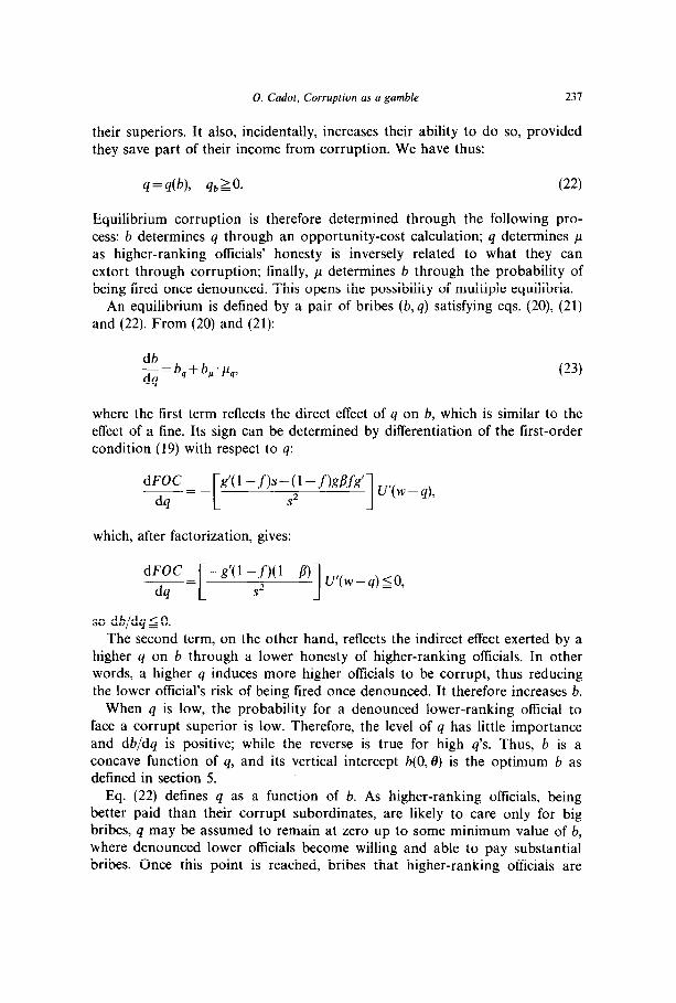
Equilibrium corruption is therefore determined through the following pro- cess: b determines q through an opportunity-cost calculation; q determines p as higher-ranking offtcials’ honesty is inversely related to what they can extort through corruption; finally, p determines b through the probability of being fired once denounced. This opens the possibility of multiple equilibria.

An equilibrium is defined by a pair of bribes (b,q) satisfying eqs. (20), (21) and (22). From (20) and (21):

db -=b,+b;p,,, dq

(23)

where the first term reflects the direct effect of q on b, which is similar to the effect of a tine. Its sign can be determined by differentiation of the first-order condition (19) with respect to q:

dFOC g’(1 -f)s-(1 -f)gPfs’ --= _ dq s2 1 U,(w_q) 2

which, after factorization, gives:

dFOC -g’(l -f)(l-P) p= dq s2 1 U’(w_q)50 3

so db/dq 5 0. The second term, on the other hand, reflects the indirect effect exerted by a

higher q on b through a lower honesty of higher-ranking officials. In other words, a higher q induces more higher officials to be corrupt, thus reducing the lower official’s risk of being fired once denounced. It therefore increases b.

When q is low, the probability for a denounced lower-ranking official to face a corrupt superior is low. Therefore, the level of q has little importance and db/dq is positive; while the reverse is true for high q’s Thus, b is a concave function of q, and its vertical intercept b(O,tl) is the optimum b as defined in section 5.

Eq. (22) defines q as a function of b. As higher-ranking officials, being better paid than their corrupt subordinates, are likely to care only for big bribes, q may be assumed to remain at zero up to some minimum value of b, where denounced lower officials become willing and able to pay substantial bribes. Once this point is reached, bribes that higher-ranking officials are

23X 0. Cndol, Corruption as a gamble

able to demand from their subordinates in any one case of denunciation are not directly bounded by the amount of bribery involved in the case. In fact, if a case has led to denunciation, the bribe h has not been paid; therefore 4 is determined. rather, by the expected discounted value of future wage and bribe income for the lower-ranking official, which is likely to be higher than h. So for h 2 hmi”, we have q(h) > h. The function defined by eq. (22) may therefore be expected to have the shape illustrated in fig. 4. The same curve is labelled h*(q) in fig. 5. where the axes have been flipped around. Fig. 5 brings together h*(q) and h(q, 6), which is eq. (20) where !r has been substituted away using (21).

Two distinct equilibria appear now. The first one, at point Ei in fig. 5, is the solution of the model presented in section 5. it involves a non-zero amount of corruption at the low level of the administration, but none at higher levels, as q; =O. The second equilibrium, at point Ez, corresponds to the pair (h;, q;), where both h; and q; are non-zero. It is therefore characterized by more petty bribery (h% >b;) encouraged by a positive amount of higher-level corruption. Thus, the solution of the model analysed in

sections 5 and 6 of this paper is but one among several solutions of the more genera1 model of section 7. The occurrence of multiple equilibria shows how situations of widespread corruption may tend to perpetuate themselves. while, in other cases, the same may be true of traditions of honesty. Moreover, it helps showing that such contrasts, inexplicable in appearance, are not necessarily attributable to different degrees of morality.

8. Concluding remarks

As pointed out by Lui (1986), dynamic considerations are an essential ingredient of any mode1 of corruption, as risk is always one of the characteristics of the business, and risk is best described in a dynamic

Q

q(b)

/

/ /

/ /

/ /

/ /

/ /

/ /

/

,/I’ ./’ I

bmin

Fig. 4


b b*(q)

%, 8)

91 e =o 4;

Fig. 5

context. The model presented in this paper has the advantage of embodying such a dynamic structure within a very simple recursive framework. It also allows for useful comparative-statics results to be easily derived; in particular, it highlights the relationship between the wage of government officials and their power. As the shadow value of the permit granted by officials may be interpreted as an index of their power, a constant degree of corruption defines an equilibrium relationship between wage and power. This has important consequences for policy. The simultaneous occurrence of low wages and strong powers - regulatory or other ~ in the hands of an administration creates a basic incentive for corruption, a phenomenon that has been noticed in many Third World economies: and when such incentives exist, the usefulness of repressive policies is uncertain. This presumption is reinforced by the result of appendix B, which shows that if crime 1s a lottery and criminals are gamblers, the effect of harsh penalties may fall short of the expectations of policymakers.

The model also helps showing how corruption is a contagious phenomenon. Once the incentive for petty corruption is created. the latter tends to develop upstream through self-interested complicity. This. in turn, creates through impunity a favourable environment for the growth of bribery. Corruption thus creates complex relationships of vassalage, protection and clientelism, based on bribery and blackmail. These relationships, though originally based on the civil service’s hierarchy, tend to bypass it and to distort normai channels of power and information. ‘This is one of the most perverse effects of generalized corruption.

Finally, corruption is, in the present modei, a gamble in the sense that government ofticials face risk each time they ask for a bribe. This puts a hmir on their rapaciousness. However, there IS no such mechanism at play in the case of higher-ranking officials, whose appetite is bounded only by the


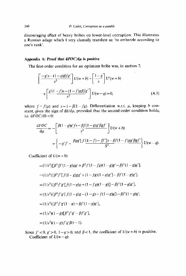
discouraging effect of heavy bribes on lower-level corruption. This illustrates a Russian adage which I very clumsily translate as: ‘to embezzle according to one’s rank’.

Appendix A: Proof that dFOC/dp is positive

The first-order condition for an optimum bribe was, in section 7:

+ L g’(l -fW(l -fkPfg’ s* 1 u(w_q)=o > (A.11

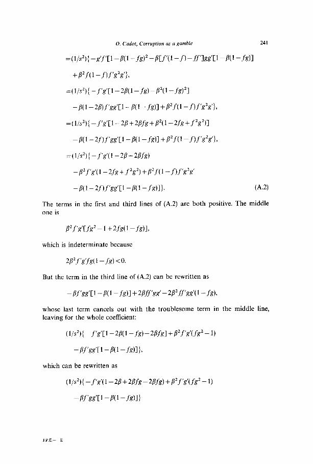
where f =f(p) and s = 1 - j?( 1 -fg). Differentiation w.r.t. p, keeping b constant, gives the sign of db/dp, provided that the second-order condition holds, i.e. dFOC/db < 0:

dFOC fi( ’ - g)g’f’ - pf( ’ - g)g’pgf ’ -= _ dp S2 1 u(~ + b)

+ _g,f,_ &s’Cf’(l -f)-ff’ls-ml -fkg’W’ i S2 I ww - 4).

Coefficient of U( w + b):

=Ws2)CPZ.ff’(1 -dgg’+P2f’(l -“ml -g)g’-ml -g)g’l,

=Ws2){P2f’CfU -&x’+(l --fd(l -sk’l-m-Y1 -dg’l,

=u/S*){B*f’dCfu -gk+U -fd(l -s)l -Bf’(l -dg’j,

=(1/~*){B*f’dCf(1 -&-Cl -d-“01 -_gkl-Iv-Y1 -EM,

=u/S2){B2f’g’u -g)-WC1 -_gk’j,

=(l/s2)(l -g)CB2f'g'-Wg'l,

=( l/?)( 1 -g)f’g’fl(t- 1).

Since f’ < 0, g’ > 0, 1 -g > 0, and fi < 1, the coefficient of U(w + b) is positive. Coefficient of U(w - 4):


=W)( -s’f’Cl -B(l -fs)‘-BCf’U -f)-ff’lss’C1 -B(l -fdl

+ B’f( 1 - “W’s’s’L

=U/s2){ -f’g’Cl -Ml -.k-P’U -m21

-B(l -Wxf’&Cl -B(l -f&d1 +B’f(l -f)f’g’s’L

=(l/?){ -f’g’[l -2fi+2fifg+flZ(1-22fg+f2g2)]

-P(l-2f)f’gg’Cf -P(l -.fdl +B’f(l -f)f’s’dI?

=W2ef’g’(l -2P+Wfd

-P’f’g’(l -2fg+f2g2)+B2f(l-_f)f’g2g’

-B(l -Tf)f’&Cl -Kl -fs)lI. 64.2)

The terms in the first and third lines of (A.2) are both positive. The middle one is

B’f ‘g’Cfg’ - 1 + 2fg( 1 - fdl,

which is indeterminate because

2P2f’g’fg( 1 - fg) < 0.

But the term in the third line of (A.2) can be rewritten as

- Wgg’C 1 - B( 1 - fdl + w.Yf’& - W2ff’&( 1 - fsh

whose last term cancels out with the troublesome term in the middle line, leaving for the whole coefficient:

(1/S2){-f’g’C1-2B(1-fg)-28~gl+B2f’g’(fg2--1)

-Wkx’Cl-8(1 -fg)l~~

which can be rewritten as

( W2) I- f’g’( 1 - 28 + Wfg - Wfid + P2f’&?(fg2 - 1)

-W&Cl -BU -.fm

J.P.E.- E


or

(l/s~)(-f’g’(1-228)+p2f’g’(fg2--)-~Bf’gg’[:I-~(I-fg)l},

which is positive. So the whole expression is positive.

Appendix B

Throughout sections 4 and 5, it has been assumed that all corrupt officials have the same degree of risk-aversion, so that they all act alike. A more plausible assumption is that they differ in this respect, their individual degrees of risk-aversion following a distribution f: The derivation of a typical candidate’s cutoff value is now slightly more complicated. His expected income is maximized with respect to c, and is defined by the following equation (applying, as before, to a good candidate):

11 +(l-p,)(l--h) j(l-b)f(b)db+j.tEY(c)f.(b)db

0 c

which means that

{l-r(l-h)[l-F(c)]jEY(c)=p,h+(l-h)j(l-b)f(h)db, 0

where F(.) is the c.d.f. of c. So

p$+(l-h&l-h)f(b)db {l-t(l-h)[l-F(c)]}. 0 II

The first-order condition defining c is

(l-c)f(c){l-t(l-h)[l-F(c)]}- p&+(1-$1~b)f(b)db i

cf(c)

(1-O -WC1 -f(cm2 = 0.

This implicitly defines, as before, c as a function of the candidate’s parameters and prior beliefs, and the official’s calculations can be carried out in the same way. It is often noticed that people in a hurry are those most willing to pay high bribes. This can be checked by differentiating the Iirst- order condition with respect to the candidate’s discount rate. Denote the derivative of EU(c) w.r.t. c by EU,. .The f.o.c. is thus EU,=O, and further denote its numerator by N, and its denominator by D:


EU,,=( -N/D2) aD/at+(l/D) aN/at.

The first term is zero when the expression is evaluated at EU,=O. So

E U,, = (l/D) aN/at

=(l/D)(l-h) -(I-h)[l-F(c)](l-c)f(c) i

p,h+(l-h)~(l-b)f(b)db

so co,

dcJdt= -EV,,IEU,,<O,

provided that the second-order condition holds. Since t = l/(1 +r), dc/dr>O. The assumption that corrupt officials differ by their degree of risk-aversion,

together with the earlier result that db/dA<O, can also be used to assess the effect of a policy of increased punishments. To make matters clear, drastic simplifications are needed.

Assume that:

(A.l) There is a non-zero probability of error (i.e. of convicting an innocent) in any judiciary system.

(A.2) The ex-ante probability of conviction in any one case is a decreasing function of the number of pieces of evidence required.

Define the degree of arbitrariness of a judiciary system as the probability of an error weighted by the severity of punishment. An increase in the latter, if it is to maintain the same degree of arbitrariness, has to come with an increase in the burden of proof, i.e. in simple terms, in the number of pieces of evidence required. This may come either either formally or informally, through more careful examination of each case. Then by (A.2), an increase in the severity of punishment reduces the ex ante probability of conviction. Denote the former by E and the latter by p (thus p here represents the probability of being convicted for a corrupt official). We have pE < 0. Rewrite the official’s problem as

my EU=[ 1 _kipp)] u(w+h)+[ 1 +yl _p)] U(--E).

The f.o.c. is

EUb= [l -p;lp:p),2 {U(w+b)-(l-f)U(-&)}+l_~~Pp) ti’(w+b),


WPbP EUbE=[l -/I(1 -p),3 W(w+b)-(1 -B)w-41

- CI_8(:_p)l’C(1-P)PbU’(-c)+P,C”(W+b)l, which is negative for ‘sufftciently concave’ utility functions. So db/de<O and an increase in punishment does have a deterrence effect, at least on sufliciently risk-averse individuals. But even among people who are somehow deterred by the change in punishments, its impact will not lead to uniform reactions. In fact, its effect is likely to be rather small, since it can be shown, with the help of an example, that the people least deterred by the change are the least risk-averse individuals, i.e. those who are most corrupt (since it has been shown earlier that db/dA CO). Suppose that the utility function of an individual official is, again, the familiar constant-risk-aversion function: U(Y)= -exp(-AY). Then

+&{(l -j3)pbeAE(1 +AE)+p,e-A’“+b)[l -(w+b)Al},

where n,=2ap,p,/[l-P(1-p)13 and AZ= -l/Cl-/3(1-p)‘. So dEU,,/dA<O, and EU,,<O. This means that an increase in punishments deters mainly petty corruption. The deterrence effect of heavier punishments is therefore likely to be disappointingly small, unless society is willing to accept hitting harder on innocents as well as guilty, which, in the long run, seems hardly sustainable as a policy to fight crime.

References

Becker, G.S., 1968, Crime and punishment: An economic approach, Journal of Political Economy, MarchhApril.

Becker, G. and G. Stigler, 1974, Law enforcement, malfeasance and compensation of enforcers, Journal of Legal Studies 3, l-19.

Bayley, D.H., 1966, The effects of corruption in a developing nation, Western Political Quarterly 4, 719-132.

Broadus, J.M., 1976, Corruption and regulation, Yale University, unpublished Ph.D. dissertation. Johnson, O.E.G., 1975, An economic analysis of corrupt government, with special application to

less developed countries, Kyklos 28, 47-61. Krueger, A.O., 1974, The political economy of the rent-seeking society, American Economic

Review, June. Lui, F.T., 1985, An equilibrium queueing model of bribery, Journal of Political Economy, Aug.,

76CL781.

Lui, F.T., 1986, A dynamic model of corruption deterrence, Journal of Public Economics, Dec., l-22.

Rose-Ackerman, S., 1975, The economics of corruption, Journal of Public Economics 4, 187-203. Rose-Ackerman, S., 1978, Corruption, a study in political economy (Academic Press, N.Y.). Rose-Ackerman, S., 1986, Reforming public bureaucracy through economic incentives?, Journal

of Law, Economics and Organization 2, Spring, 13 l-l 61.

Date post:	23-Nov-2021
Category:	Documents
Upload:	others
View:	3 times
Download:	1 times

CORRUPTION AS A GAMBLE - Harvard University

Documents