Corso di Laurea in Ingegneria Civile Tesi di Laurea...

UNIVERSITÀ DEGLI STUDI DI PADOVA

DIPARTIMENTO DI INGEGNERIA CIVILE EDILE E

AMBIENTALE ICEA

Corso di Laurea in Ingegneria Civile

Tesi di Laurea Magistrale

An algorithm for numerical modelling of Cross-Laminated Timber structures

LAUREANDO:

Gabriele D’Aronco

RELATORE:

Prof. Ing. Roberto Scotta

CORRELATORE:

Prof. Ing. Sergio Oller

ANNO ACCADEMICO 2014 - 2015

ABSTRACT

Cross-laminated timber, also known as X-Lam or CLT, is well established in

Europe as a construction material. Recently, implementation of X-Lam products and

systems has begun in countries such as Canada, United States, Australia and New

Zealand. So far, no relevant design codes for X-Lam construction were published in

Europe, therefore an extensive research on the field of cross-laminated timber is being

performed by research groups in Europe and overseas. Experimental test results are

required for development of design methods and for verification of design models

accuracy.

This thesis is part of a large research project on the development of a software

for the modelling of CLT structures, including analysis, calculation, design and

verification of connections and panels. It was born as collaboration between Padua

University and Barcelona‟s CIMNE (International Centre for Numerical Methods in

Engineering). The research project started with the thesis “Una procedura numerica per

il progetto di edifici in Xlam” by Massimiliano Zecchetto, which develops a software,

using MATLAB interface, only for 2D linear elastic analysis. Follows the phase started

in March 2015, consisting in extending the 2D software to a 3D one, with the severity

caused by modelling in three dimensions. This phase is developed as a common project

and described in this thesis and in “Pre-process for numerical analysis of Cross

Laminated Timber Structures” by Alessandra Ferrandino.

The final aim of the software is to enable the modelling of an X-Lam structure in

the most efficient and reliable way, taking into account its peculiarities. Modelling of

CLT buildings lies into properly model the connections between panels. Through the

connections modelling, the final aim is to enable the check of preliminarily designed

connections or to find them iteratively, starting from hypothetical or random

connections.

This common project develops the pre-process and analysis phases of the 3D

software that allows the automatic modelling of connections between X-Lam panels. To

Abstract

achieve the goal, a new problem type for GiD interface and a new application for

KRATOS framework have been performed. The problem type enables the user to model

a CLT structure, starting from the creation of the geometry and the assignation of

numeric entities (beam, shell, etc.) to geometric ones, having defined the material, and

assigning loads and boundary conditions. The user does not need to create manually the

connections, as conversely needs for all commercial FEM software currently available;

he just set the connection properties to the different sides of the panels. The creation of

the connections is made automatically, keeping into account different typologies of

connections and assembling of Cross-Lam panels. The problem type is special for X-

Lam structures, meaning that all features are intentionally studied for this kind of

structures and the software architecture is planned for future developments of the post-

process phase.

It can be concluded that sound bases for the pre-process and analysis phases of

the software have been laid. However, future research is required to develop the post-

process and verification phases of the research project.

ACKNOWLEDGMENTS

I would like to thank all the people that helped me in the realization of this work.

First of all I want to express my gratitude to my advisor, Prof. Roberto Scotta, which

gives me the possibility to make this great experience at the CIMNE for developing my

thesis.

I would like to express my gratitude to all the CIMNE staff, especially to my co-

advisor, Prof. Sergio Oller and my tutor Prof. Antonia Larese De Tetto, for their

hospitality and guidance during this period. I had also the possibility to know Dr.

Massimo Petracca and I would like to thank him for his constant and endless help in the

realization of this thesis.

In these years I had the possibility to meet a lot of people that let me unforgettable

memories and experiences; I really would like to thank the friends from Friuli, the

group from Padova and the friends from Barcelona. Between them a special mention is

necessary for: Andrea, Giacomo, Katia, Marco, Rachele, Pietro, Valentina and Gisela

for their understanding, encouragement and constantly presence in the good and in the

hard times.

Last but not least, my deepest gratitude is directed to my parents: Mauro and Carla,

which have supported me in every choice in these years of the University and have

made all of this possible.

Gabriele D‟Aronco

Padova, 2015

CONTENTS

CHAPTER 1 ................................................................................................................................ 1

INTRODUCTION ....................................................................................................................... 1

1.1 Research background and motivation ................................................................................. 1

1.3 Thesis structure ................................................................................................................... 6

CHAPTER 2 ................................................................................................................................ 9

GENERALITIES ABOUT X-LAM TECHNOLOGY ............................................................. 9

2.1 X-Lam panels manufacturing ............................................................................................ 12

2.2 Advantages of X-Lam technology .................................................................................... 14

2.3 X-Lam connection systems ............................................................................................... 18

2.4 X-Lam structural applications ........................................................................................... 29

CHAPTER 3 .............................................................................................................................. 33

KRATOS STRUCTURE AND GENERAL INFORMATION ABOUT GID, C++ AND PYTHON .................................................................................................................................... 33

3.1 Kratos Structure ................................................................................................................ 33

3.1.1Kernel and Applications .............................................................................................. 33

3.1.2 Basic Components ...................................................................................................... 34

3.1.2.1 Object Oriented Design ....................................................................................... 35

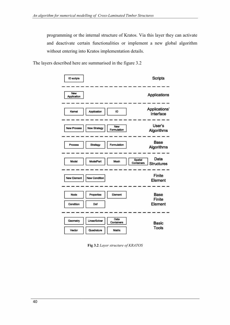
3.1.2.2 Multi-Layered Design ......................................................................................... 38

3.1.3 Node and Nodal Data ................................................................................................. 41

3.1.3.1 The Node ............................................................................................................. 41

3.1.3.2 Kratos Variables .................................................................................................. 41

3.1.3.3 Types of Nodal Data ........................................................................................... 41

3.1.3.5 Non-historical database: Values .......................................................................... 42

3.1.3.6 Degrees of Freedom ............................................................................................ 43

3.1.4 Elements and Conditions ............................................................................................ 43

3.1.4.1 The Geometry class ............................................................................................. 43

3.1.4.2 Properties ............................................................................................................. 44

3.1.5 Strategies and Processes ............................................................................................. 44

3.1.5.1 Time scheme ....................................................................................................... 44

3.1.5.2 Builder and solver ............................................................................................... 45

Contents

3.1.5.3 Strategy ............................................................................................................... 45

3.1.5.4 Process ................................................................................................................. 45

3.1.5.5 Utilities ................................................................................................................ 45

3.1.5.6 Python solvers ..................................................................................................... 46

3.1.6 Workflow ................................................................................................................... 46

3.1.6.1 The Model Part (.mdpa) file ................................................................................ 46

3.1.6.2 The Python script ................................................................................................ 46

3.2 General about GiD ............................................................................................................ 47

3.3 General about C++ ............................................................................................................ 47

3.4 General about Python language ......................................................................................... 48

CHAPTER 4 .............................................................................................................................. 51

IMPLEMENTATION OF X-LAM DRIVER APPLICATION ............................................ 51

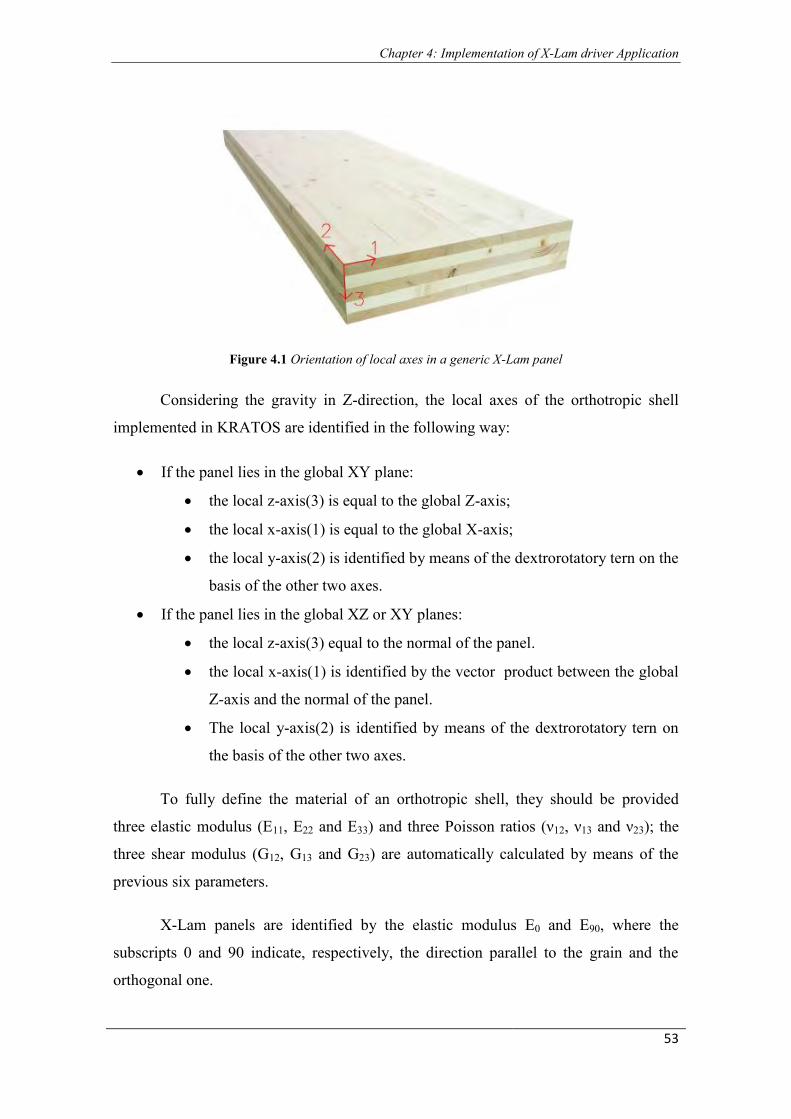
4.1 Modelling of an X-Lam structure ...................................................................................... 51

4.1.2 Modelling of X-Lam panels ....................................................................................... 52

4.1.3 Modelling of the connections ..................................................................................... 54

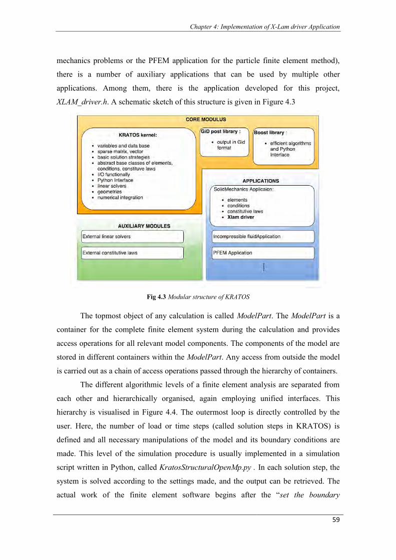
4.2 Introduction of Xlam driver.h .......................................................................................... 58

4.2.2 KratosOpenMP- workflow concept of the analysis.................................................... 58

4.3 Structure of the application ............................................................................................... 62

4.3.1 Reading of the Model Part and the Elements ID ........................................................ 65

4.3.1.1 Reading of the Nodes .......................................................................................... 65

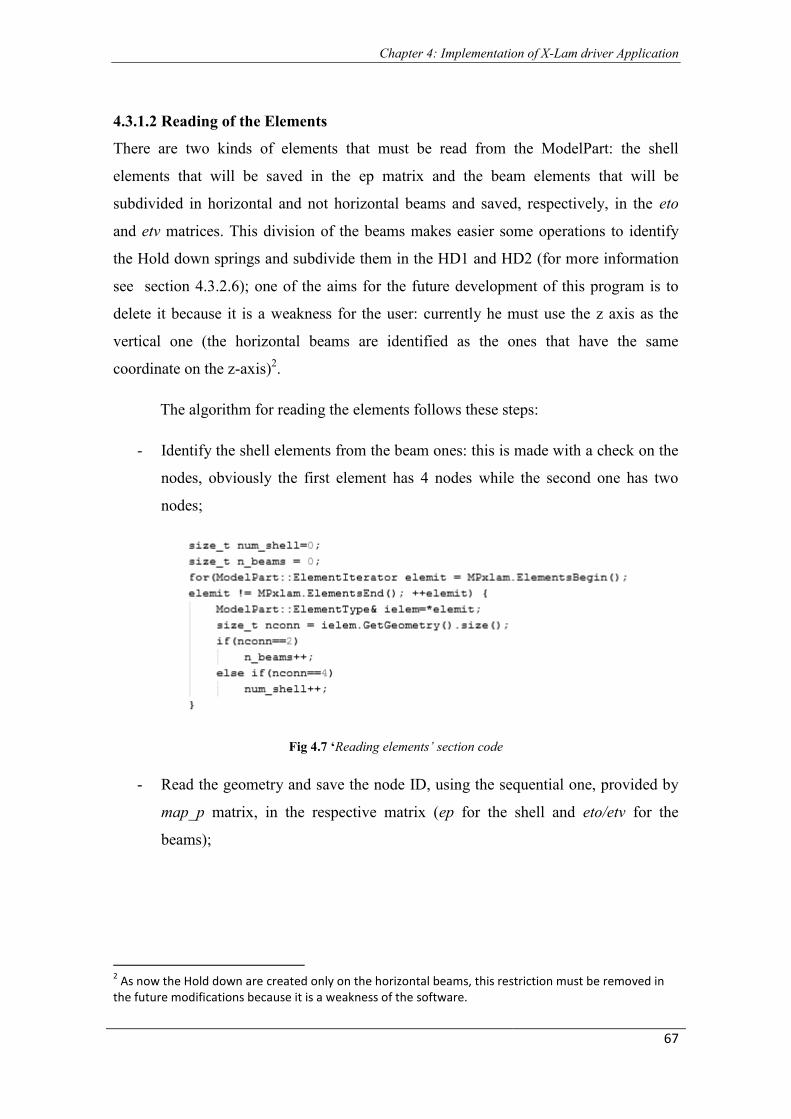
4.3.1.2 Reading of the Elements ..................................................................................... 67

4.3.2 Modification of the ModelPart ................................................................................... 69

4.3.2.1 Nodes Duplication ............................................................................................... 70

4.3.2.2 Building of the geometric elements direction ..................................................... 73

4.3.2.3 Geometric creation of the spring elements .......................................................... 75

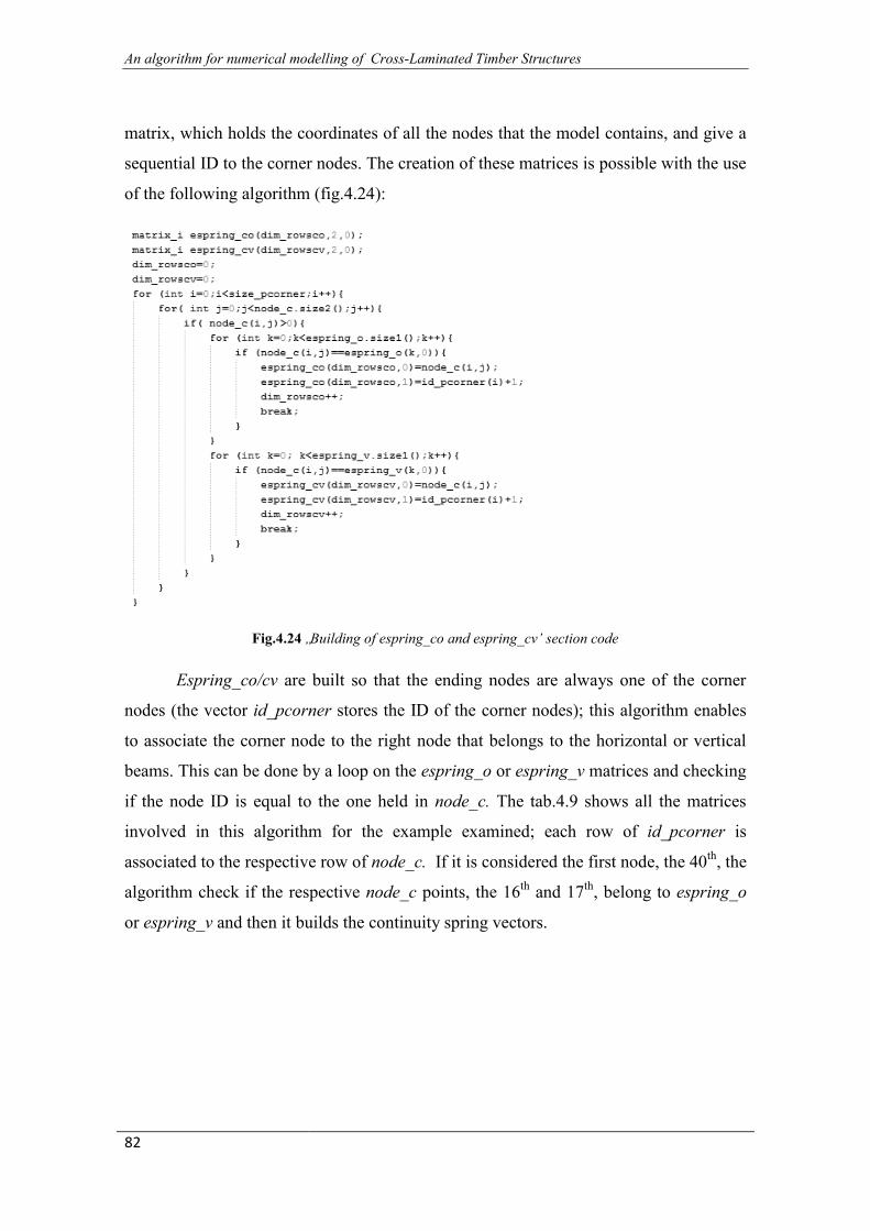
4.3.2.4 Creation of the continuity spring elements .......................................................... 80

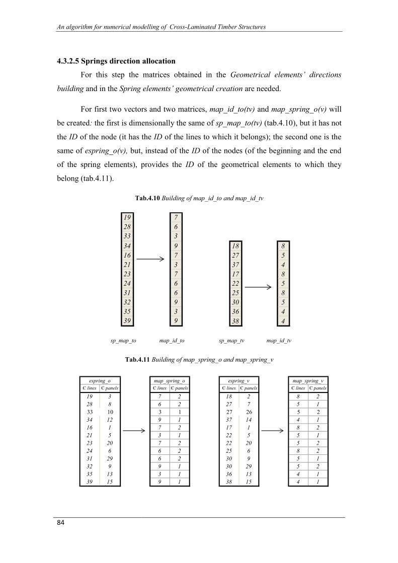
4.3.2.5 Springs direction allocation ................................................................................. 84

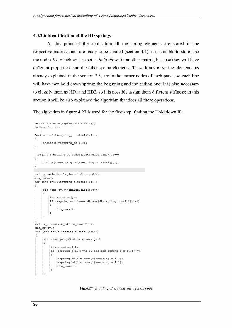
4.3.2.6 Identification of the HD springs .......................................................................... 86

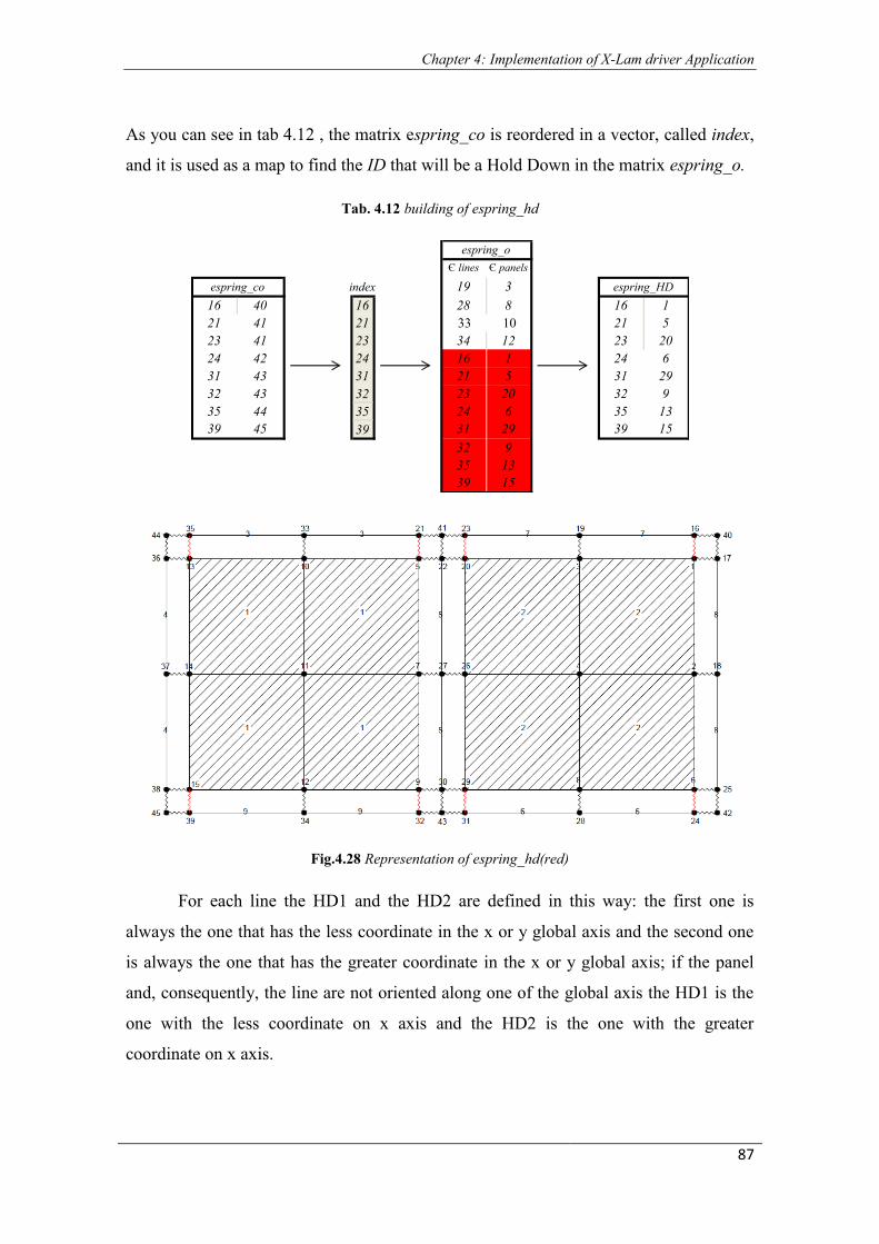
4.3.2.7 Assignment of the stiffness according to the mesh ............................................. 88

4.3.3 Updating of the ModelPart and Creation of the new elements .................................. 91

4.3.3.1 Updating of the ModelPart .................................................................................. 91

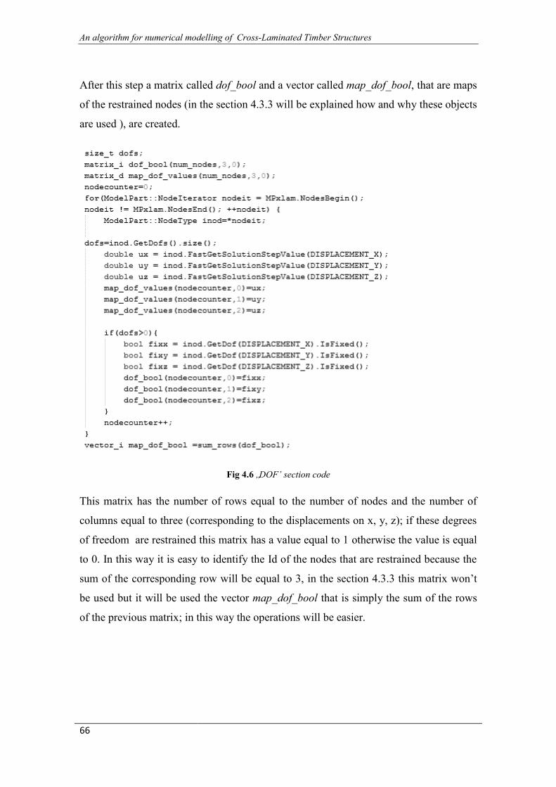
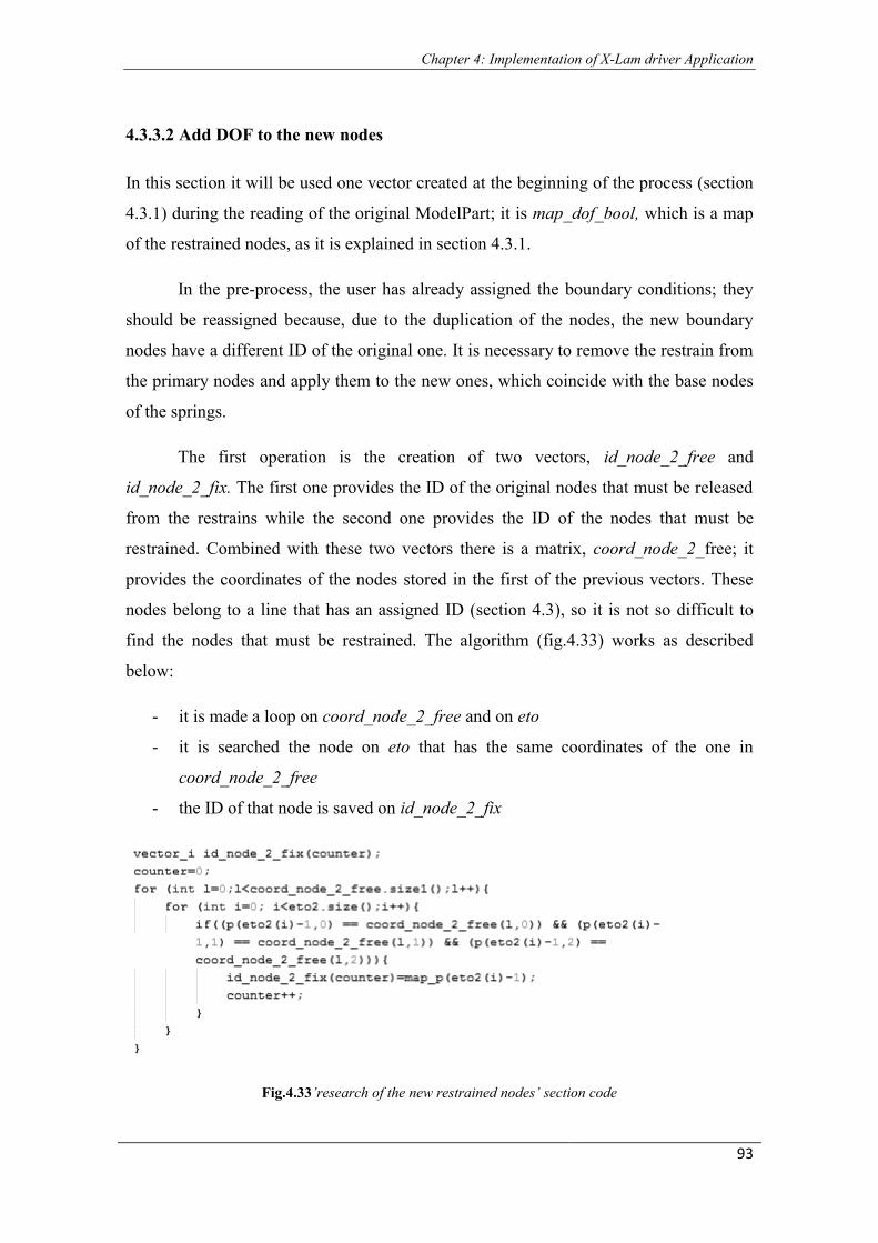
4.3.3.2 Add DOF to the new nodes ................................................................................. 93

4.3.3.3 Creation and Uploading of the Spring elements.................................................. 95

CHAPTER 5 .............................................................................................................................. 99

Contents

VALIDATION EXAMPLES .................................................................................................... 99

5.1 Introduction ....................................................................................................................... 99

5.2 First case study ................................................................................................................ 100

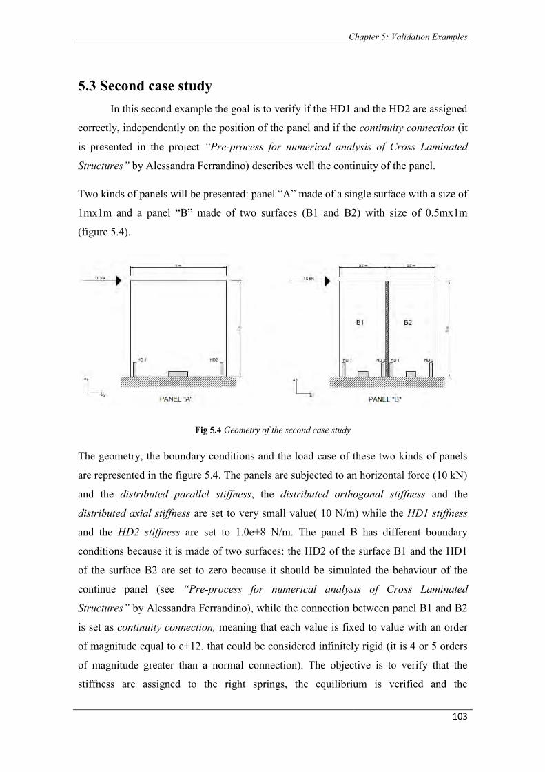
5.3 Second case study ........................................................................................................... 103

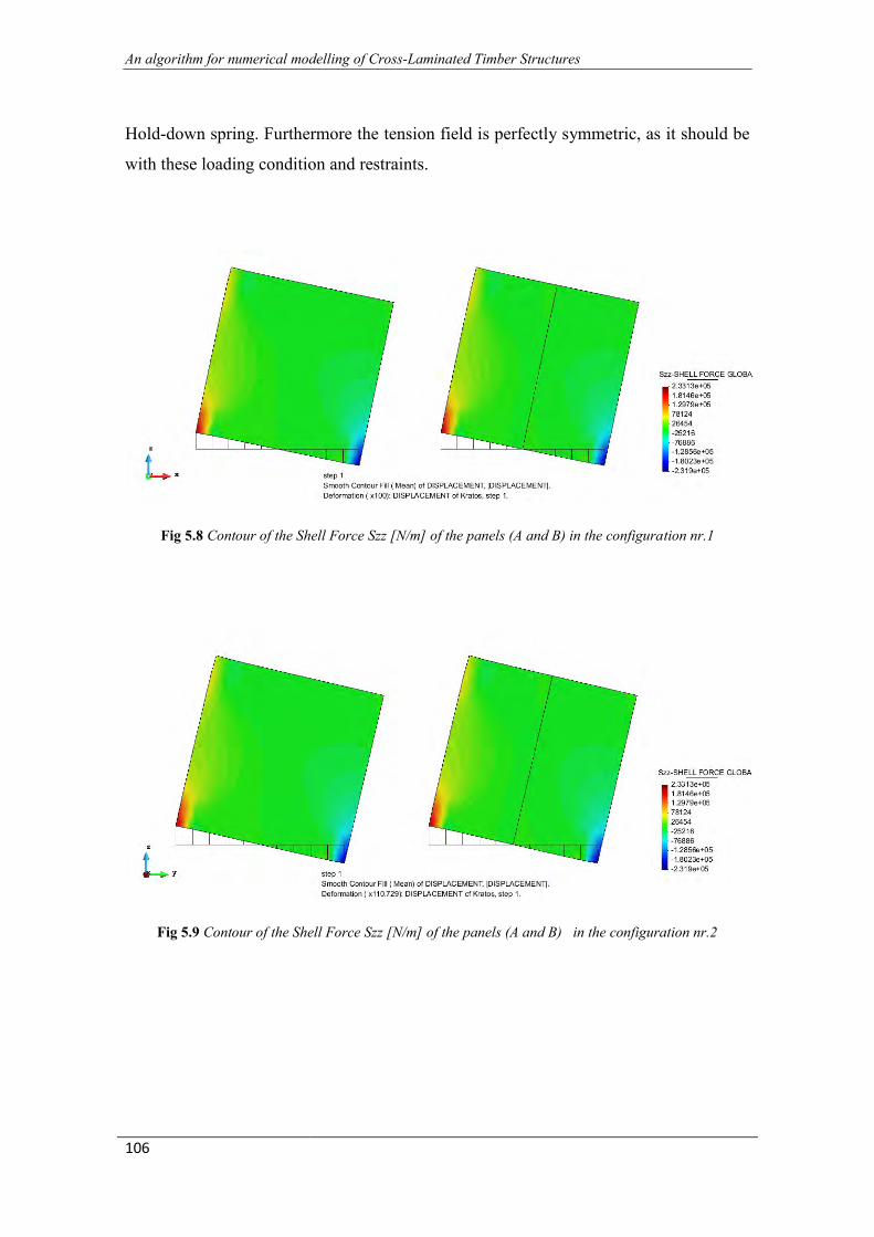
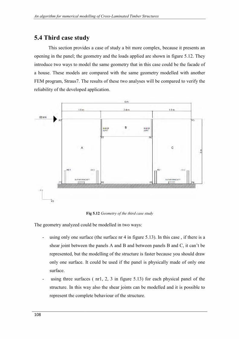
5.4 Third case study .............................................................................................................. 108

CHAPTER 6 ............................................................................................................................ 117

ANALYSIS OF A COMPLEX STRUCURE ........................................................................ 117

6.1 Example introduction ...................................................................................................... 117

6.2 Preliminary design phase ................................................................................................ 120

6.2.1 Static design of X-Lam walls and slabs ................................................................... 120

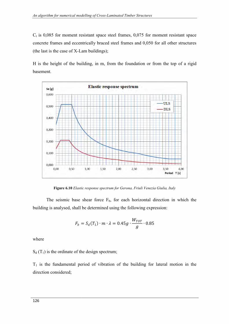
6.2.2 Seismic design of X-Lam walls and slabs ................................................................ 123

6.2.3 Equivalent static analysis ......................................................................................... 124

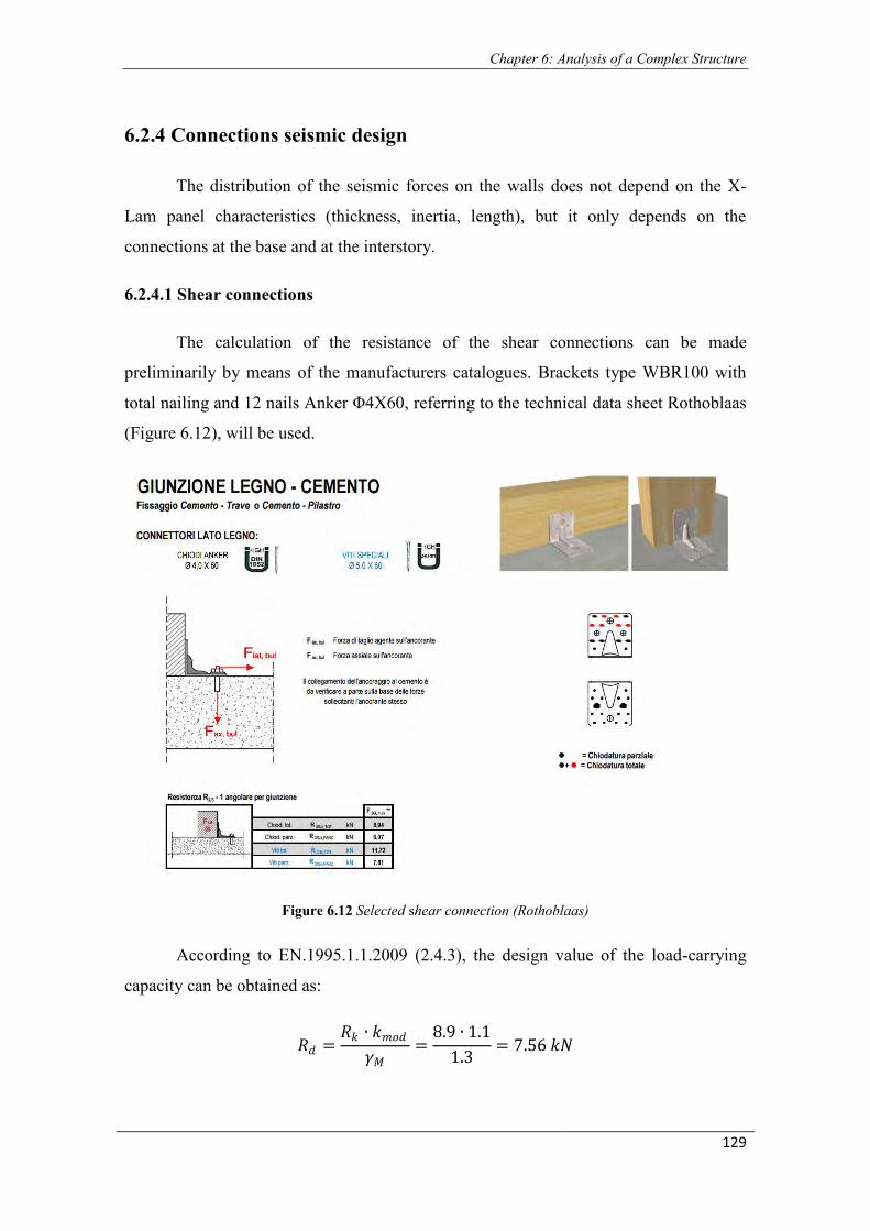
6.2.4 Connections seismic design...................................................................................... 129

6.2.4.1 Shear connections .............................................................................................. 129

6.2.4.2 Tension connections .......................................................................................... 130

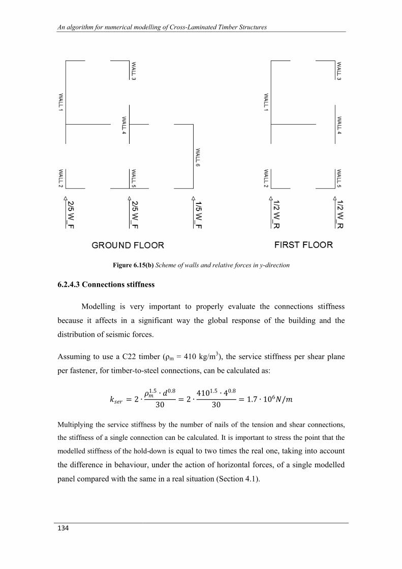
6.2.4.3 Connections stiffness ......................................................................................... 134

6.3 Modelling ........................................................................................................................ 135

6.3.1 Geometry .................................................................................................................. 135

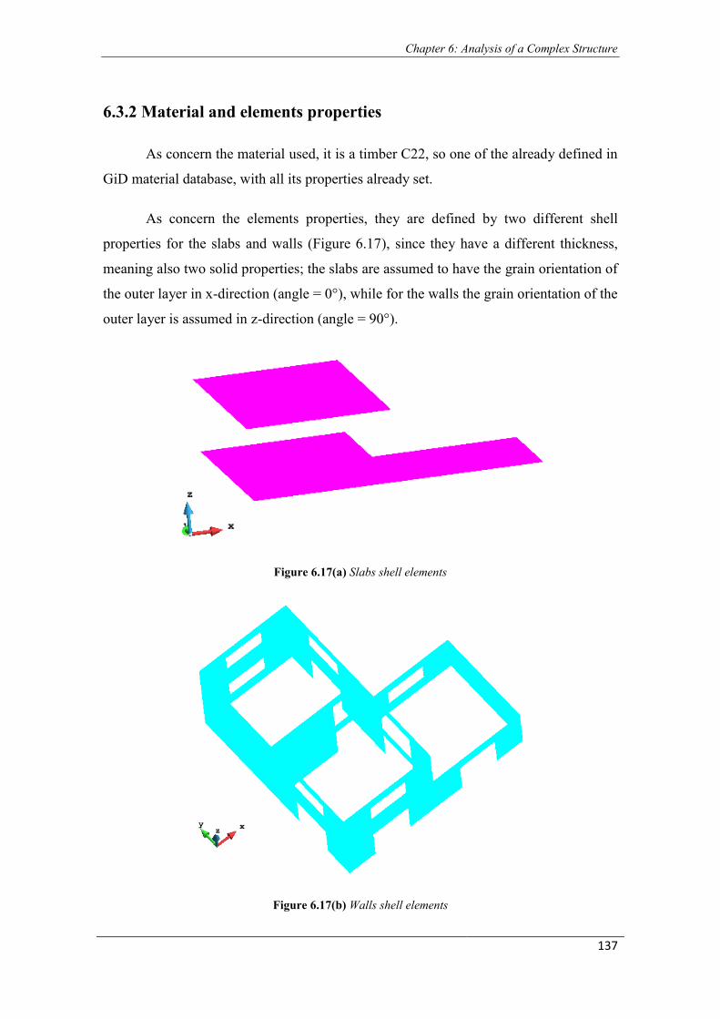
6.3.2 Material and elements properties ............................................................................. 137

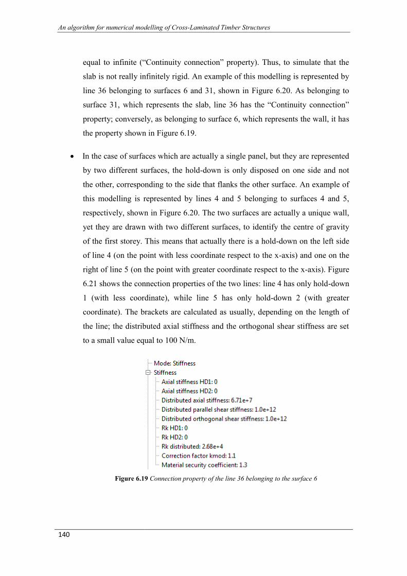
6.3.3 Connection properties .............................................................................................. 139

6.3.3 Boundary conditions and loads ................................................................................ 142

6.4 Results ............................................................................................................................. 143

6.4.1 Structure discretization ............................................................................................. 143

6.4.2 Displacement Field ................................................................................................... 144

6.4.3 Tension Field ............................................................................................................ 147

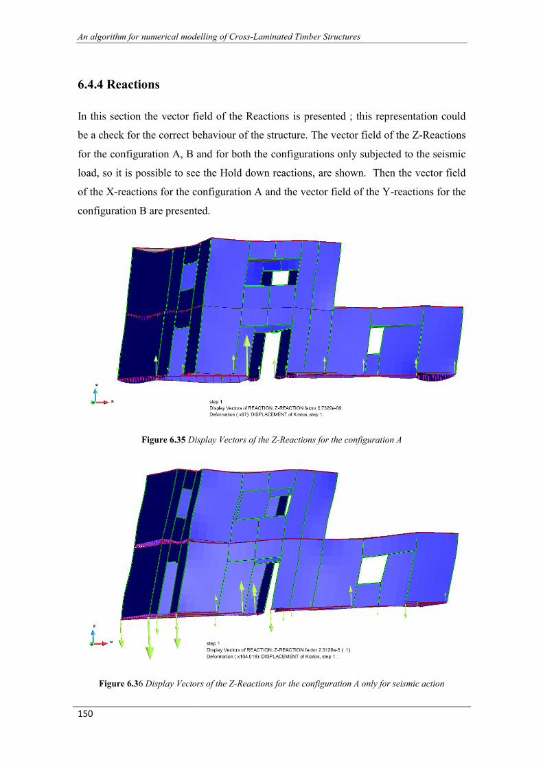
6.4.4 Reactions .................................................................................................................. 150

CHAPTER 7 ............................................................................................................................ 153

CONCLUSION ........................................................................................................................ 153

7.1 Main contributions .......................................................................................................... 153

7.2 Recommendations for further research ........................................................................... 154

REFERENCES ........................................................................................................................ 156

1

CHAPTER 1

INTRODUCTION

1.1 Research background and motivation

Wood as a building material possesses some inherent characteristics that make

timber structures particularly suited for the use in regions with a high seismic risk, both

due to material properties, such as lightness and load bearing capacity (good weight-to-

strength-ratio), and to system properties, like ductility and energy dissipation. Recently,

there have been new developments with prefabricated timber elements, which aim to

address modern building requirements for cost, constructability and structural

performance. Massive cross-laminated timber panels (X-Lam), which can be used as

wall panels, floor panels or roof panels in timber buildings, are becoming a stronger and

economically valid alternative to traditional masonry or concrete buildings in Europe,

and recently also overseas. Especially in seismic-prone countries, X-lam buildings are

gaining more and more popularity. However, due to relatively short time since this

wood engineered product has been launched to the market, the knowledge about cross-

lam as a structural material is still limited. In recent years, several research projects

around Europe and in North America have been launched, with an aim to better

understand the potential of cross-lam technology as a seismic resistant construction

system.

Still limited is also the knowledge about the modelling of X-Lam structures,

reason why a large research project started to investigate the development of a software

for the analysis, calculation, design and verification of X-Lam structures. This project

was born as collaboration between Padua University and Barcelona‟s CIMNE

(International Centre for Numerical Methods in Engineering). Modelling of CLT

buildings lies into properly model the connections between panels; they play an

essential role in maintaining the integrity of the timber structure and providing strength,

An algorithm for numerical modelling of Cross-Laminated Timber Structures

2

stiffness, stability and ductility to the structure. The connections may be modelled with

punctual or distributed spring elements, or with shell elements. Anyway the goal is to

provide the needed flexibility to the connecting points, to avoid a fully unreal behaviour

of the building, being the panels very rigid in comparison to the anchoring connections.

Through the connections modelling, the final aim is to enable the check of preliminarily

designed connections or to find them iteratively, starting from hypothetical or random

connections.

The research project started with the thesis “Una procedura numerica per il

progetto di edifici in Xlam” by Massimiliano Zecchetto, which develops a software,

using MATLAB interface, only for 2D linear elastic analysis. Follows the phase started

in March 2015, consisting in extending the 2D software to a 3D one, with the severity

caused by modelling in three dimensions. This phase is described in this thesis and in in

“Pre-process for numerical analysis of Cross Laminated Timber Structures” by

Alessandra Ferrandino; it consists in the pre-process and analysis phases of the 3D

software. Further research is still needed to develop the post-process and verification

phases.

The development of this research project arises from the need to model and

calculate an X-Lam structure in the most efficient and reliable way, taking into account

its peculiarities. Proper modelling strategy comes out in the development of a special

software. This comes from the non-adaptability to X-Lam technology of the established

procedures for numerical modelling adopted for other types of buildings. Nowadays the

commercial FEM software available do not provide an automatic way to model a CLT

structure. All software, whatever technique is chosen, only enable to model the

connections manually; e.g. if they are modelled with punctual springs, the user must

duplicate the nodes and create the spring elements one by one at the pre-process

interface. Follows that, if the structure is big and complex as it can be a real one, the use

of these software could require time and cost expenditure and it may cause several

errors because of its complexity: hundreds or thousands, if not more, may be the nodes,

elements and properties that should be assigned. The aim of this research project is

exactly to provide a software that allows the automatic modelling of connections

Chapter 1: Introduction

3

between X-Lam panels, trying to avoid the human error and the cost in doing it

manually.

The most convenient strategy for modelling X-Lam structures has to be defined.

Such strategy must be suitable for automatic generation of numerical models and must

have the ability of keeping into account all the possible typologies of connections and

assembling of Cross-Lam panels. In view of future evolution of the research, the

possibility of non-linear behaviour of joints and optimal automatic design via iterative

solutions has to be accomplished too.

1.2 Objectives and scope

The focus of this thesis is on the continuation of the research project on the

development of a software for the modelling of CLT structures, including analysis,

calculation, design and verification of connections and panels. The research work will

include the pre-process phase and the analysis one, the first of which is discussed in in


Alessandra Ferrandino, the second one in this thesis.

The procedure is developed using GiD as interface support and processor and

KRATOS Multiphysics as FEM framework. Relatively to the pre-process phase, the

work involved in programming and numerical implementation of the interface and the

data needed for the analysis, by creating a problem type. Relatively to the analysis

phase, the work consisted in the development of the whole procedure of connections

modelling, by creating a new application in Kratos.

Considering the numerical and computational aspects of X-Lam structures,

several are the limits and issues that make it difficult to create models fully

representative of their real behaviour.

Cross-Lam wall panels are very rigid in comparison to the anchoring

connections, so most of the flexibility is concentrated precisely in the latter. To

correctly model the building, avoiding to make it too rigid, the connections are


4

modelled with punctual spring elements. They enable to simulate the behaviour of the

different kind of connections available in X-Lam technology.

Additionally, a limit lies in the behaviour of the spring elements to use in the

modelling. The behaviour of a CLT structure in static conditions can be assimilated to a

contact problem because the walls are supported all along their lower side by the soil. In

this condition, the walls only work to compression, they do not offer any resistance to

tension. The possible lifting of the walls, which may occur in seismic conditions, is

resisted by the hold-down connections that offer the tension resistance to the walls. To

simulate properly the contact problem, the springs should present a non-linear

constitutive law in axial direction. Alternatively, the problem can be considered non-

linear for the material, considering the hold-down as a material non-resistant to

compression and the soil as a material non-reactive to traction. Within this project, the

springs present a linear elastic constitutive law, leading to the need of modifying the

hold-down stiffness compared to the real one. This is to take into account the difference

in behaviour, under the action of horizontal forces, of a single modelled panel compared

with the same in a real situation. Therefore, being the spring elements currently added in

Kratos only implemented with linear elastic constitutive law, the analysis is always

considered linear elastic.

In reference to the behaviour of a single X-Lam panel, this is an orthotropic

rather than an isotropic material. This is due to the different total thickness of the layers

in longitudinal and transversal direction and to the difference in value of the elastic

modulus of the timber, which is one order of magnitude greater in the direction parallel

to the grain than in the transversal direction. These two topics lead to adopt an elastic

orthotropic constitutive law for the shell elements.

The research work developed in this common project concerns the creation of a

new problem type, especial for X-Lam structures. It enables the user to model a CLT

structure, starting from the creation of the geometry and the assignation of numeric

entities (beam, shell, ecc) to geometric ones, having defined the material, and assigning

loads and boundary conditions. The user does not need to create manually the

connections, he just set the connection properties to the different sides of the panels.

Also the punctual connections (hold-down) are assigned at the interface to the lines;


5

conversely, in the analysis they are assigned only to the extreme points of the panel

side.

The creation of the connections is made automatically: an abstract offset is

applied between each surface and line, or, better, between each border shell in which the

surface is discretized and beam elements. The information about the connection

property is stored at interface level to the line (geometric entity), which is discretized,

depending on the mesh, in one or more beams (numeric entities). The offset (Figure 1.1)

implies the duplication of the nodes that belong to both the beams and shells. It has zero

distance to allow an easy management of the nodes, since the duplicated nodes will

have the same coordinates of the original ones.

Figure 1.1 Example of an offset surface

Therefore, spring elements, with the stiffness values inserted by the user at the interface,

are used to join nodes with equal coordinates. The beam elements, necessary for the

duplication of the nodes, are considered fake elements, if not set as curbs at the

interface. Their geometric and structural properties are so that their presence is

negligible in the analysis of the structure. Figure 1.2 shows the springs connecting the

shells and beams.

Figure 1.2 Exploded view of a panel edge


6

The pre-process phase, concerning the creation of a new problem type in GiD, is

described in the thesis “Pre-process for numerical analysis of Cross Laminated Timber

Structures” by Alessandra Ferrandino. It enables, at interface level, the creation of

geometry and the assignation of elements properties, material, loads, boundary

conditions and, above all, connection properties. Moreover, it allows the creation of

suitable input data files for the analysis and the modelling of the panels as orthotropic

shells with composite cross section.

The analysis phase, concerning the numerical changes in Kratos framework, is

described in this thesis. It consists in the implementation of the spring elements and the

numerical procedure for the automatic modelling of connections, meaning duplication

of the panels‟ border nodes and their joint by means of the spring elements.

1.3 Thesis structure

A brief summary of each chapter of the thesis is given in this section. In each

chapter, the first section overviews general information about the chapter topic; in

subsequent sections, theoretical and numerical investigations are described.

Chapter 2 provides an overview of general information about cross-laminated

timber technology. First, description of cross-lam panels and their application in

construction is introduced. Then, typical X-Lam connection systems are presented and

their significance in cross-lam technology is described. A state-of-the-art of cross-lam

timber application is highlighted at the end of this Chapter.

Chapter 3 provides an overview about all the tools used for the project. For first

there is a widely description of the structure of KRATOS and of his tools, then some

background information about his pre-processor, GiD and at the end there is a quick

explanation about the programming languages used, C++ and Python.

Chapter 4 provides for first a description of the philosophy of modelling chosen

for an X-Lam structure; then there is a detailed explanation of the implementation of the

application developed in the Kratos Framework for the nodes duplication and the spring

creation. Each section of the application is deeply described and a simple example is

provided for helping in the comprehension of the numerical procedure.


7

Chapter 5 provides some numerical examples to validate the application

developed; three examples will be presented: two of them to check the assignment of

the properties of the springs and the last one for comparing the displacement and

tension field with the results provided from a commercial program.

Chapter 6 is a presentation of the calculation of a real X-Lam structure; the goal

is simply to show how the new problem type and the calculation work for a complex

structure. Thus, the numerical modelling of the structure and the results, obtained with

the Problem-type developed will be presented.

9

CHAPTER 2

GENERALITIES ABOUT X-LAM TECHNOLOGY

Cross laminated timber (X-Lam or CLT) is an engineered wood product

fabricated by adhering and compressing wood layers called lamellas in perpendicular

grain orientations to form a solid panel. Wood layers are glued together on their wide

faces and, usually, on the narrow faces as well. X-Lam technology was invented and

developed in central Europe in the early 1990„s and since then it has been gaining

increased popularity in residential and non-residential applications. The number of

buildings constructed using X-Lam panels as the main structural system has seen

exponential growth in the last decade, and market share for X-Lam construction is

expected to continue to escalate in the future. The European experience showed that X-

Lam construction can be competitive, particularly in mid-rise and high-rise buildings

due to its easy handling during construction and a high level of prefabrication. Recently,

X-Lam was introduced also overseas, in North America, Australia and in New Zealand.

A number of production plants have been established or they are proposed to be built in

aforementioned countries.

Figure 2.1 Cross-laminated timber panel (ETA-06/0138, 2006)


10

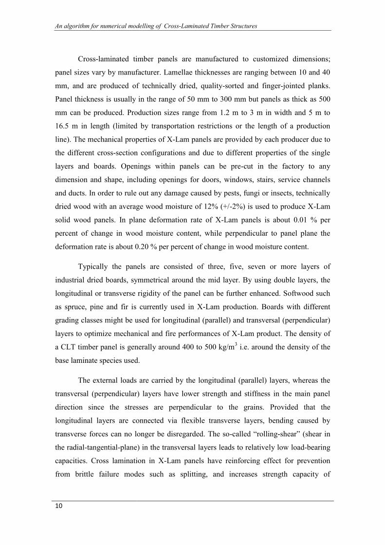
Cross-laminated timber panels are manufactured to customized dimensions;

panel sizes vary by manufacturer. Lamellae thicknesses are ranging between 10 and 40

mm, and are produced of technically dried, quality-sorted and finger-jointed planks.

Panel thickness is usually in the range of 50 mm to 300 mm but panels as thick as 500

mm can be produced. Production sizes range from 1.2 m to 3 m in width and 5 m to

16.5 m in length (limited by transportation restrictions or the length of a production

line). The mechanical properties of X-Lam panels are provided by each producer due to

the different cross-section configurations and due to different properties of the single

layers and boards. Openings within panels can be pre-cut in the factory to any

dimension and shape, including openings for doors, windows, stairs, service channels

and ducts. In order to rule out any damage caused by pests, fungi or insects, technically

dried wood with an average wood moisture of 12% (+/-2%) is used to produce X-Lam

solid wood panels. In plane deformation rate of X-Lam panels is about 0.01 % per

percent of change in wood moisture content, while perpendicular to panel plane the

deformation rate is about 0.20 % per percent of change in wood moisture content.

Typically the panels are consisted of three, five, seven or more layers of

industrial dried boards, symmetrical around the mid layer. By using double layers, the

longitudinal or transverse rigidity of the panel can be further enhanced. Softwood such

as spruce, pine and fir is currently used in X-Lam production. Boards with different

grading classes might be used for longitudinal (parallel) and transversal (perpendicular)

layers to optimize mechanical and fire performances of X-Lam product. The density of

a CLT timber panel is generally around 400 to 500 kg/m3 i.e. around the density of the

base laminate species used.

The external loads are carried by the longitudinal (parallel) layers, whereas the

transversal (perpendicular) layers have lower strength and stiffness in the main panel

direction since the stresses are perpendicular to the grains. Provided that the

longitudinal layers are connected via flexible transverse layers, bending caused by

transverse forces can no longer be disregarded. The so-called “rolling-shear” (shear in

the radial-tangential-plane) in the transversal layers leads to relatively low load-bearing

capacities. Cross lamination in X-Lam panels have reinforcing effect for prevention

from brittle failure modes such as splitting, and increases strength capacity of

Chapter 2: General about X-Lam Technology

11

connections. The cross-laminating process provides improved dimensional stability to

the product which allows for prefabrication of long and wide panels. Additionally,

cross-laminating provides relatively high in-plane and out-of-plane strength and

stiffness properties, giving it two-way action capabilities similar to a reinforced concrete

slab.

Figure 2.2 Examples of different cross-sections of X-Lam panels (ETA-06/0138 2006)

By varying the number of layers as well as the lumber species, grade and

thickness, X-Lam panels can be used in various assembly types such as walls, floors,

roofs, elevator shafts, stairways etc. The wall and floor panels may be left exposed in

the interior, which provides additional aesthetic attributes. The panels are used as

prefabricated building components which can speed up construction practices or allow

for off-site construction. While X-Lam panels act as two-way slabs, the stronger

direction follows the grain of the outer layers. For example, when used for walls, X-

Lam is installed so the boards on the outer layer of the panel have their grain running


12

vertically. When panels are used in floor and roof applications, they are installed so the

boards on the outer layer run parallel to the span direction.

Panels may be connected to each other with half-lapped, single or double splines

made from engineered wood products. Dowel-type mechanical fasteners such as nails,

screws, dowels and bolts, or bearing-type (e.g., split rings, shear plates) connectors are

used to connect X-Lam panels. Typical X-Lam connections will be presented more in

detail in Section 2.3 of this Chapter.

2.1 X-Lam panels manufacturing Currently there are no standards in Europe that cover X-Lam manufacturing or

installation. However, various X-Lam products have a European Technical Approval

(ETA) that allows manufacturers to place CE marking. The approval process includes

preparation of a European Technical Approval Guideline (ETAG) that contains specific

requirements of the product as well as test procedures for evaluating the product prior to

submission to the European Organization for Technical Approvals (EOTA). Finally, the

ETA allows manufacturers to place CE marking (Conformité Européenne) on their

products.

In the USA, the American National Standards Institute (ANSI) recently

approved ANSI/APA PRG 320-2012 Standard for Performance-Rated Cross-Laminated

Timber (ANSI/APA PRG 320-2012, 2012). This Standard covers manufacturing,

qualification and quality assurance requirements for X-Lam products. Key stakeholders

included X-Lam manufacturers, distributors, designers, users, building code regulators,

and government agencies.

In general, the production of cross-laminated timber panels follows the

following procedure:

Selection of species

The base species of timber used for X-Lam panels depend on the region where it is

manufactured. For X-Lam manufactured in Austria and Germany spruce is the main

species used; pine and larch can also be used on request. X-Lam plants in Canada are


13

likely to use S-P-F (spruce pine fir) species. Whilst production is yet to occur in

Australia and New Zealand, the timber species likely to be used is radiata pine.

Timber laminates grouping

Individual seasoned dimensional timbers are used, generally softwood and usually

finger jointed along their length to obtain the desired lengths and quality. Individual

timbers can be edged bonded together to form a timber plate before further assembly

into the final panel.

Adhesive application

Generally the choice of adhesives is dependent on manufacturers but the new

polyurethane (PUR) adhesives are normally used as they are formaldehyde and solvent

free. Occasionally, and manufacturer dependent, melamine urea formaldehyde and

phenol-resorcinol-formaldehyde adhesives could be used. Both face and edge gluing

can be applied.

Panel assembly and arrangement

The main difference that occurs between X-Lam manufacturers is the treatment of

individual layers. Some manufacturers edge bond the individual dimensional timber

together to form a layer before pressing each layer into the final X-Lam panel. Other

manufacturers just face bond individual dimensional timber in layers and press all of

them together into the final X-Lam panel in the one operation. Panel sizes vary by

manufacturer and application, as mentioned in the beginning in this Chapter.

Pressing

Gluing at high pressure reduces the timbers expansion and shrinkage potential to a

negligible level, thus the right pressure is essential. Hydraulic presses are normally

employed, however, use of vacuum and compressed air presses is also possible,

depending on panel thickness and the adhesive used. Vertical and horizontal pressings

can be applied.


14

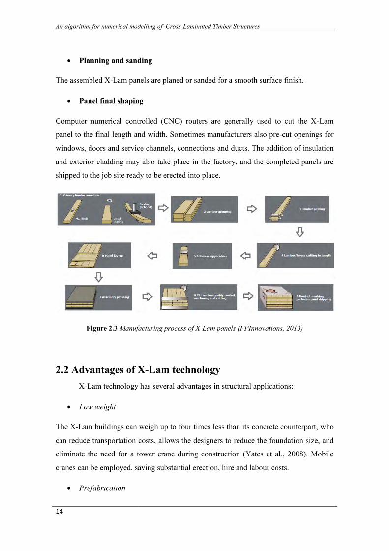
Planning and sanding

The assembled X-Lam panels are planed or sanded for a smooth surface finish.

Panel final shaping

Computer numerical controlled (CNC) routers are generally used to cut the X-Lam

panel to the final length and width. Sometimes manufacturers also pre-cut openings for

windows, doors and service channels, connections and ducts. The addition of insulation

and exterior cladding may also take place in the factory, and the completed panels are

shipped to the job site ready to be erected into place.

Figure 2.3 Manufacturing process of X-Lam panels (FPInnovations, 2013)

2.2 Advantages of X-Lam technology X-Lam technology has several advantages in structural applications:

Low weight

The X-Lam buildings can weigh up to four times less than its concrete counterpart, who

can reduce transportation costs, allows the designers to reduce the foundation size, and

eliminate the need for a tower crane during construction (Yates et al., 2008). Mobile

cranes can be employed, saving substantial erection, hire and labour costs.

Prefabrication


15

The prefabricated nature of X-Lam technology permits high precision in terms of

dimensional accuracy due to CNC controlled cutting and quality controlled production.

Wall, floor and roof elements can be pre-cut, including openings for doors, windows,

stairs, service channels and ducts. Insulation and finishes can also be applied prior to

installation, reducing demand for skilled workers on site. Construction process is

characterized by increased safety on the construction site, faster project completion and

availability for occupancy in a shorter time. For example, it took four carpenters just

nine weeks to erect nine stories and the entire construction process was reduced from 72

weeks to 49 weeks (Yates et al., 2008) compared to a traditional reinforced concrete

building. In addition, there is less disruption to the surrounding community and less

waste is produced. As most of the work occurs off-site at the factory, there is a lower

demand for skilled workers on-site.

Easy handling and erection

Handling the X-Lam panels requires smaller cranes which also influences on the lower

cost of a building construction. One of the biggest benefits of using X-Lam panels is

that the structure can be built quickly and efficiently. Because panels are designed for

specific end-use applications, they are often delivered and erected using a “just-in-time”

construction method, making X-Lam ideal for projects with limited on-site storage

capacity. Panels are usually loaded into the truck at the manufacturing plant in the

sequence that they will be required for installation on site. Where it is not possible to

install X-Lam panels immediately, they can be off-loaded and stored off the ground

under a waterproof covering until required. Due to the light weight of the panels it is

also common to use the building itself as a place to temporarily store panels. It is also

possible to assemble elements or modules of the building off-site and deliver completed

segments of the building to the site. This speeds up the construction process even

further. Panels are lifted into place using pre-inserted hooks.

Flexibility in architectural implementation

Versatility of X-Lam technology comes from the fact that panels can be used for many

different assemblies (wall, floor, roof, stairs etc.) just by varying the thickness. X-Lam

construction system can be combined also with other timber structural systems such as


16

light timber frames, post-and-beam heavy timber system and glue-laminated timber. In

addition, X-Lam elements are compatible with other building materials such as steel,

concrete and glass. Compared to traditional light wood-frame construction methods,

which rely on plywood sheathing over wood studs (walls) or rafters and beams (roof),

the use of X-Lam panels offers an alternative in the form of a single component that is

load bearing and provides an aesthetically pleasing finished surface. Depending on its

intended use, X-Lam panels can be used for either visible or hidden construction

applications. Its ability to be used as either a panellized or a modular system makes it

ideally suited for additions to existing buildings or their upgrade. Good span-to-depth

ratio allows shallow floors and slender construction elements can increase the net

building are.

Static properties

High in-plane and out-of-plane strength and stiffness properties of X-Lam panels enable

in-plane stability of the panels and lack of susceptibility to soft-story failures. The

cross-lamination provides relatively high strength and stiffness properties in both

directions, giving it a two-way action capability similar to a reinforced concrete slab.

Seismic performance

In terms of seismic performance, timber buildings in general perform well because

wood is relatively light as a construction material, thus inertial forces caused by

earthquakes are lower than in case of buildings made of other materials. High ductility

and energy dissipation capacities of X-Lam buildings, together with sufficient strength

capacity, make this construction system very effective at resisting lateral forces caused

by earthquake ground motions.

Fire resistance

X-Lam assemblies have inherently excellent fire-resistance due to the thickness of

panels, which when exposed to fire, slow down the heat propagation within the cross-

section and char at a slow and predictable rate (0.67 mm/min according to ETA -

06/0138, 2006). Once formed, this char protects the wood from further degradation,

helping to maintain structural integrity of the building. In addition, X-Lam structures


17

also tend not to have as many concealed spaces within floor and wall assemblies, which

reduce the risk of a fire spreading. Fire performance of X-Lam panels can also be

enhanced by lining with fire resisting gypsum boards and, in case of floor panels,

additional layers and coverings. A demonstration test conducted by IVALSA on a full

scale, three-storey X-Lam building confirmed that X-Lam panels protected by one layer

of gypsum board were able to withstand the burn out of the room contents without fire

spread to adjacent rooms or floors (Frangi et al., 2008).

Thermal performance

Cross-lam panels have the same fundamental thermal insulation and thermal mass

properties as the wood from which they are made (thermal conductivity λ = 0.13

W/(m*K) according to EN 12524, 2000). Wood has a low thermal conductivity so

reduces problems such as thermal bridging from the internal to the external

environments and the other way around, thus reducing heat transfer and energy wastage.

Acoustic performance

Solid wood panels offer acoustical advantages when used for floor and wall systems.

When used in conjunction with insulation and gypsum board, it is possible for an X-

Lam building to exceed code requirements related to the acoustical performance of

floors and walls.

Dimensional stability

The crosswise arrangement of the longitudinal and transverse layers reduces the

swelling and shrinkage of the wood in the plane of the panel to an insignificant

minimum and considerably increases the static load-carrying capacity and dimensional

stability.

Durability

Generally due to the quick erection time of X-Lam based systems, the short term

exposure of X-Lam panels to weather is not an issue. Short term and occasional

exposure to water will not have long term effect on X-Lam panels. During construction

wall elements may be protected with vapour barriers or the building‟s scaffolding can


18

be wrapped to form this protection. Other strategies could be employed such as coating

system for the construction period only. Long-term exposure of X-Lam panels to

weather is not recommended.

Sustainable and environmental friendly building material

As with all wood products, the benefits of X-Lam include the fact that wood grows

naturally, using solar energy and it is the only major building material that is renewable

and sustainable. It also has a low carbon footprint, because the panels continue to store

carbon absorbed during the tree„s growing cycle and because of the greenhouse gas

emissions avoided by not using products that require large amounts of fossil fuels to

manufacture. Harvesting from sustainably managed forests contribute to efficient use of

the resource. Many of the recent structures built from CLT benefit from these

environmental considerations. For example, two mid-rise residential projects in London

used the fact that wood stores carbon and that substantial greenhouse gas emission were

avoided by substituting cross-lam in place of concrete or steel to get preferential

approval from local planning authorities (Yates et al., 2008).

Recycling and reuse

X-Lam panels can also be recycled and reused for the same or for a different purpose.

Structural flexibility of the panels is very wide as well as their durability, thus enabling

panels to be reused. For example, after a series of shake table tests on a 7-storey SOFIE

building in Japan, the building was disassembled and the panels were shipped back to

Italy. The panels were stored for a couple of years, before they were used as main load-

carrying elements in the newly developed prototype of a sustainable modular house unit

made of X-Lam panels (Briani et al., 2012).

2.3 X-Lam connection systems X-Lam wall panels are very rigid in comparison to the anchoring connections, so

most of the flexibility is concentrated in the connections. Thus, connections play an

essential role in maintaining the integrity of the timber structure and providing strength,

stiffness, stability and ductility to the structure. The structural efficiency of the floor


19

system acting as a diaphragm and that of walls in resisting lateral loads depends on the

efficiency of the fastening systems and connection details used to connect individual

panels and assemblies. Consequently, they require detailed attention by designers. In

addition, damages and failures in X-Lam buildings during a seismic event are localized

in connections; thus, structural repairs after an earthquake are relatively easy and cost

effective.

When structural members are attached with fasteners or some other types of

metal hardware, such joints are referred to as “mechanical connections”. Currently,

there is a wide variety of mechanical fasteners and many different types of joint details

that can be used for panel to panel connections in X-Lam assemblies or to connect X-

Lam panels to other wood-based, concrete or steel elements in hybrid construction. A

combination of metal hold-downs, angle brackets and self-tapping screws are typically

recommended by the X-Lam manufacturers for connecting the cross-lam panels.

Metal brackets, hold-downs, plates and straps are used to transfer forces from

walls to floors, from one level to another level, and to foundations. Hold-downs are

mainly used in the corners of wall segments and close to door opening, to resist

overturning forces that result from an earthquake or wind. On the other hand, the main

role of L-shaped metal brackets is to resist shear forces in wall panels caused by wind or

a seismic event. Nails with specific surface features such as grooves or helically

threaded nails are mostly used with perforated metal plates and brackets and installed on

the surface of the panel.

Long self-tapping screws are typically recommended by X-Lam manufacturers

due to their ease of installation along with high lateral and withdrawal capacity, which

make these fasteners popular because they can take combined axial and lateral loads.

Bolts and dowels are very common in heavy timber construction. They can also

be used in the assembly of X-Lam panels, especially for lateral loading. If installed in

the narrow face, care must be taken during the design, especially in X-Lam panels with

unglued edges between the individual planks in a layer. This could eventually

compromise the lateral resistance since there is a potential that such fasteners are driven

in the gaps.


20

However, there are other types of traditional and innovative fasteners and

fastening systems that can be used efficiently in X-Lam assemblies. The choice of the

type of connection to use depends largely on the type of assemblies to be connected,

panel configurations, and the type of structural system used in the building. With these

mechanical connections, several possibilities for assembling X-Lam panels are possible,

as shown in Figure 2.4.

Figure 2.4 Typical three-storey X-Lam building showing various connections between the X-

Lam panels


21

1. Wall-to-foundation connections

Several fastening systems are available for connecting X-Lam wall panels to steel

beams or to concrete foundations with concrete footing, which are most common for the

ground stories in X-Lam buildings.

Visible or exposed metal plates

Exterior metal plates and brackets are commonly used in such applications as there is a

variety of such metal connectors readily available on the market and due to its simple

installation. Lag screws or powder-actuated fasteners can be used to connect the metal

plate to the concrete footing or slab, while nails, lag screws or self-tapping screws are

used to connect the plate to the X-Lam panel. Exposed metal plates and fasteners need

to be protected against corrosive exterior environments. Galvanized or stainless steel

should be used in such cases. Direct contact between the concrete foundation and X-

Lam panel should be avoided in all cases. Connection details should be designed to

prevent potential moisture penetration between the metal plates and the X-Lam wall as

water may get trapped and cause potential decay of the wood.

Concealed connectors

For better fire resistance and improved aesthetics, designers sometimes prefer concealed

connection systems. This can be achieved with hidden metal plates. However, some

CNC machining work is required to produce the grooves in the X-Lam panel to conceal

the metal plates. Tight dowels or bolts can be used to attach the plates to the X-Lam

panel. In addition, some innovative types of fasteners that can be drilled through metal

and wood or other types of screws that can penetrate through both materials can also be

used for this purpose.

Wooden Profiles

Wooden profiles, which are fabricated from high density and stable materials such as

engineered wood products or high density hardwood, are commonly used for

connecting structural insulated panels (SIP) and other types of prefabricated wood-

framed walls. The major advantage of this system is the ease of assembly. The wooden

profiles are typically attached to X-Lam panels with wood screws or self-tapping screws


22

and are often used in combination with metal plates or brackets to improve the lateral

load resistance. Wooden profiles can also be used for wall-to-wall or floor-to-wall

connections.

Figure 2.5 Typical wall-to-foundation X-Lam connections: (a) Connection with an exposed

metal plate; (b) Connection with a concealed connector; (c) Connection with a wooden profile

(FPInnovations, 2013)

2. Wall-to-wall connections

2a) Parallel wall panel connection

This connection type is used to connect panels along their longitudinal edges. The

parallel wall-wall panel connection facilitates the transfer of in-plane forces (shear) and

out-of-plane forces (bending) through the wall assembly. Several connections details are

possible.

Internal splines or strips

For formation of this connection type, single or double wooden splines (strips) made of

structural composite lumber, such as laminated veneer lumber (LVL), plywood or thin

X-Lam, are used. Connection between the spline or splines and the panel edges can be


23

established using self-tapping screws, wood screws or nails. The advantage of this detail

is that it provides a double shear connection and resistance to out-of-plane loading.

However, special attention is required due to necessity of accurate profiling for the

fitting of different parts on a construction site.

Surface splines or strips

This connection detail is fairly simple connection detail that can be established quickly

on site but it only provides single shear connection. Since two sets of screws are used,

which results in doubling the number of shear planes resisting the load, a better

resistance can be achieved using this detail. Panel edges are profiled from one side for a

single surface spline or from both sides for a double surface spline. Similarly as in the

case of internal splines, structural composite lumber elements are used for strips.

Traditional fasteners such as nails, self-tapping screws, wood screws and lag screws can

be used for making the connection on site. In case of double surface spline connection,

the strength and stiffness of the connection can be increased. If SCL (structural

composite lumber) is used as the spline, the joint can be designed to resist moment for

out-of-plane loading (Augustin, 2008). Structural adhesives could be used to enhance

the strength and stiffness.

Half-lapped joint

In this connection type, long self-tapping screws are usually used to connect the panel

edges. The joint can carry normal and transverse loads but it is not considered to be a

moment resisting connection (Augustin, 2008). This connection detail is considered as

very simple, so it facilitates quick assembly of X-Lam elements. However, there is a

risk of splitting of the cross section due to concentration of tension perpendicular to

grain stresses in the notched area. This is particularly emphasized for cases where

uneven loading on the floor elements occur (Augustin, 2008).

Tube connection system

Tube connection system incorporates a profiled steel tube with holes in the X-Lam

panel. Panel elements are delivered on site with glued-in or screwed rods driven in the

plane of the two panels which are supposed to be connected. The tube connector is


24

inserted at certain locations along the edges of the panels where the metal tubes are to

be placed. The system is tightened on site using metal nuts. Usually no edge profiling

along the panel is needed as it relies principally on the pullout resistance of the screwed

or glued-in rods (Traetta, 2007).

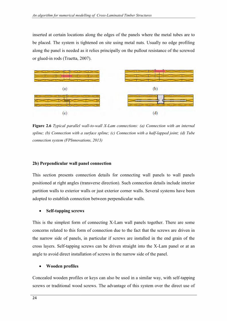
Figure 2.6 Typical parallel wall-to-wall X-Lam connections: (a) Connection with an internal

spline; (b) Connection with a surface spline; (c) Connection with a half-lapped joint; (d) Tube

connection system (FPInnovations, 2013)

2b) Perpendicular wall panel connection

This section presents connection details for connecting wall panels to wall panels

positioned at right angles (transverse direction). Such connection details include interior

partition walls to exterior walls or just exterior corner walls. Several systems have been

adopted to establish connection between perpendicular walls.

Self-tapping screws

This is the simplest form of connecting X-Lam wall panels together. There are some

concerns related to this form of connection due to the fact that the screws are driven in

the narrow side of panels, in particular if screws are installed in the end grain of the

cross layers. Self-tapping screws can be driven straight into the X-Lam panel or at an

angle to avoid direct installation of screws in the narrow side of the panel.

Wooden profiles

Concealed wooden profiles or keys can also be used in a similar way, with self-tapping

screws or traditional wood screws. The advantage of this system over the direct use of


25

self-tapping screws is the possibility of enhancing the connection resistance by driving

more wood screws to connect the profiled panel to the central wood profile which is in

turn screwed to the transverse wall.

Metal brackets

Another simple form of connecting walls in the transverse direction is the use of metal

brackets with screws or nails. This connection system is one of the simplest and most

efficient types of connection in terms of strength resulting from fastening in the

direction perpendicular to the plane of the panels or recessed. However, adding

protective membrane (i.e., gypsum board) for improved fire resistance is required.

Concealed metal plates

As previously discussed, while this system has considerable advantages over exposed

plates and brackets, especially when it comes to fire resistance, the system requires

precise profiling at the plant using CNC machining technology. Self-drilling dowels that

can penetrate through wood and steel can also be used. Metal plate thickness ranges

from 6 mm up to 12 mm.

Figure 2.7 Typical perpendicular wall-to-wall X-Lam connections: (a) Connection with self-

tapping screws; (b) Connection with a wooden profile; (c) Connection with a metal bracket; (d)

Connection with a concealed metal plate (FPInnovations, 2013)


26

3. Wall-to-floor connections

Several possibilities exist when it comes to connecting walls to the floors above,

depending on the form of structural systems (i.e., platform or balloon), on the

availability of fasteners and the degree of prefabrication.

3a) Platform construction

Self-tapping screws

The simplest method for connecting a floor or a roof to walls below is to use long self-

tapping screws driven from the X-Lam floor directly into the narrow side of the wall

edge. Self-tapping screws can also be driven at an angle to maximize the fastening

capacity in the panel edge. The same principle could be applied for connecting walls

above to floors below, where self-tapping screws are driven at an angle in the wall near

the junction with the floor. However, this type of connection has relatively low seismic

capacity in terms of strength and stiffness (Popovski, 2010).

Metal brackets

Metal L-shaped brackets are commonly used to connect floors to walls above and below

to transfer lateral loads from diaphragm to shear walls. Nails or wood screws can be

used to attach the metal brackets to the X-Lam panels. They are also used for

connecting roofs to walls.

Concealed metal plates

As discussed before, while concealed metal plates have considerable advantages over

exposed plates and brackets (especially fire resistance), the system requires precise

profiling at the plant using CNC machining technology.


27

Figure 2.8 Typical wall-to-floor X-Lam connections: (a) Connection with self-tapping screws;

(b) Connection with a metal bracket; (c) Connection with concealed metal plates

(FPInnovations, 2013)

3b) Balloon construction

In Europe, the most common type of structural form in X-Lam construction is the

platform type of system due to its simplicity in design and erection. However, in non-

residential construction, including industrial buildings, it is common to use tall walls

with an intermediate floor between the main floors of a building. So called “mezzanine

floor” is often located between the ground floor and the first floor. However, it is not

unusual to have a mezzanine in the upper floors of a building. Several attachment

options to connect X-Lam floor to a continuous X-Lam tall wall exist for such

applications. The simplest attachment detail includes the use of a wooden ledger (made

of structural composite lumber) to provide a continuous bearing support to the X-Lam

floor panels. Another type of attachment is established with the use of metal brackets.

Attachment of wooden ledger or metal brackets to the X-Lam wall and floor panels is

established through the use of screws, lag screws or nails. However, out-of-plane

bending due to wind suction could be an issue with this type of detail and designers

need to take that into account.


28

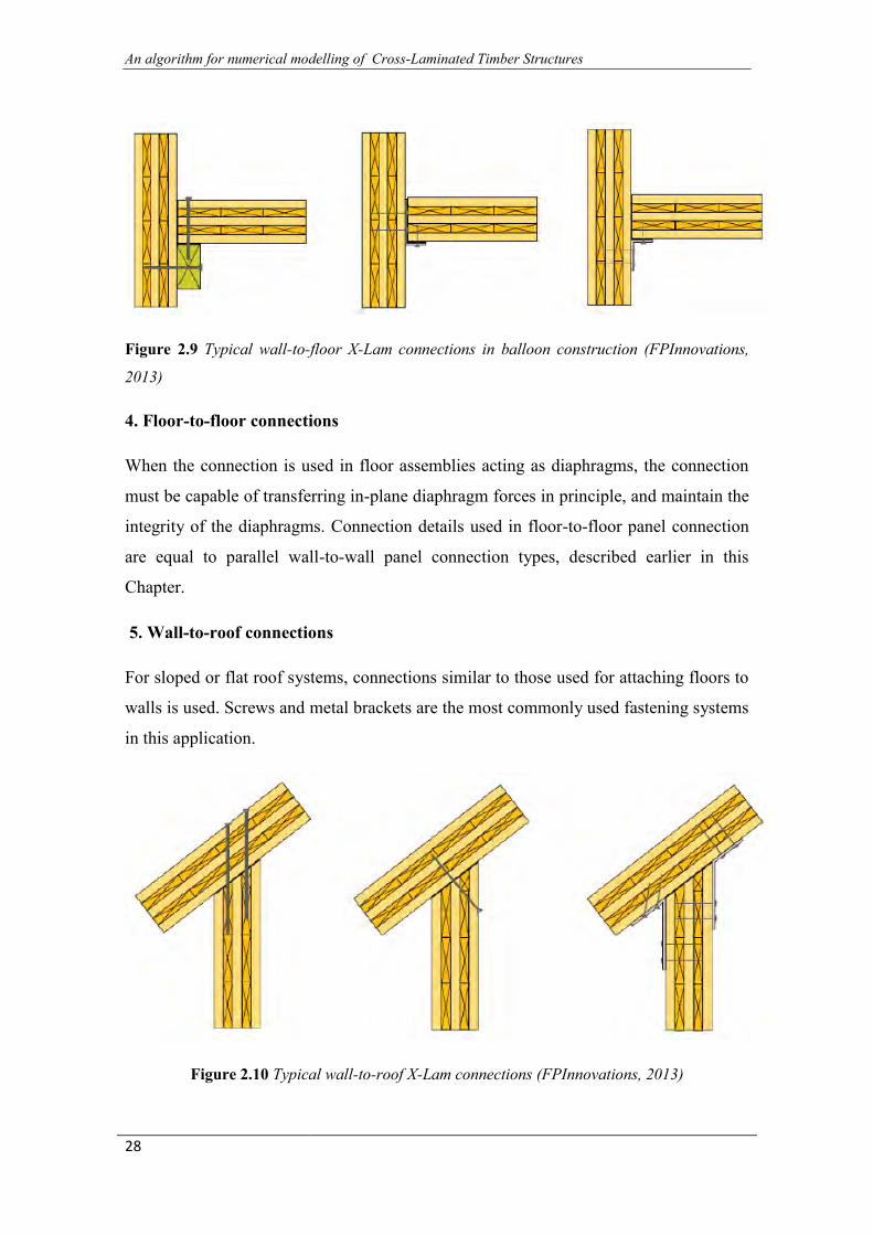
Figure 2.9 Typical wall-to-floor X-Lam connections in balloon construction (FPInnovations,

2013)

4. Floor-to-floor connections

When the connection is used in floor assemblies acting as diaphragms, the connection

must be capable of transferring in-plane diaphragm forces in principle, and maintain the

integrity of the diaphragms. Connection details used in floor-to-floor panel connection

are equal to parallel wall-to-wall panel connection types, described earlier in this

Chapter.

5. Wall-to-roof connections

For sloped or flat roof systems, connections similar to those used for attaching floors to

walls is used. Screws and metal brackets are the most commonly used fastening systems

in this application.

Figure 2.10 Typical wall-to-roof X-Lam connections (FPInnovations, 2013)


29

Innovative types of connection systems can also be used, including mechanical

and carpentry connection systems. Some interesting innovative connection systems are

finding their way to the X-Lam construction market, mostly facilitated and enabled by

CNC technology. For example, glued-in rods can be used for connections under high

longitudinal and transverse loads. HBV-Shear Connectors, a proprietary product from

Germany, can also be used to create composite floors with structural concrete over X-

Lam panels (Bathon & Bletz, 2006). Further, KNAPP system (Knapp) and Idefix

connectors (Sigha) are relatively new innovative connection systems on the market. Due

to the relatively recent introduction of X-Lam technology into the construction market,

it is expected that even more new connection types will be developed over time.

Figure 2.11 Sihga Idefix innovative connection systems (Sihga)

2.4 X-Lam structural applications This section presents an introduction to the X-Lam construction systems and

their applications. There are several ways to design and construct X-Lam buildings.

They all differ in the way the load-carrying elements (panels) are arranged, the way the

panels are connected together and by the type of wood and non-wood based materials

used. The most common forms of X-Lam construction systems are platform

construction and so called balloon construction (FPInnovations, 2013).

Platform construction in X-Lam technology is a system where the floor panels

rest directly on top of wall panels, therefore forming a platform for subsequent floors.


30

This is the most commonly used type of structural system for X-Lam assemblies for

multi-storey buildings. This includes buildings constructed with X-Lam panels only or

combining the panels with other types of wood-based products, for example glulam.

There are several advantages to this system, such as quicker erection of upper stories,

possible application of simple connection systems and well-defined load path.

Balloon construction is a type of structural system where the walls continue for a

few stories with intermediate floor assemblies attached to those walls. Due to the

limitations in the length of the X-Lam panels, this system is often used in low-rise,

commercial or industrial buildings; connections are usually more complex in this form

of construction. Balloon construction is generally less common compared to platform

construction.

X-Lam solid wood panels are used both as load-bearing, reinforcing elements

and non-load-bearing elements. Areas of application:

houses and apartment buildings

multi-storey residential buildings

public buildings

hotels and restaurants

schools and kindergartens

offices and administrative buildings

event halls

industrial and commercial buildings

reconstructions, extensions and upgrades

building retrofits

bridges

Numerous buildings using X-Lam panels have already been erected around the

world, starting in Europe, and recently some projects were realized in North America

and in Australia. In Europe, the tallest X-Lam structure to date is the 9-storey Stadthaus

residential building in London, which includes eight stories of X-Lam over one story of

concrete. At the time of the erection, in 2009, this building was the tallest wooden

residential building in the world. Short erection time, environmental benefits and cost


31

efficiency of the building illustrated how X-Lam can be a competitive system in the

marketplace (Yates et al., 2008). In 2011, another multi-storey residential building was

constructed in London, named Bridport House. It is consisted of two joined blocks, one

eight storeys high and the other five storeys high, both entirely built with X-Lam

technology, including the ground floor, which is traditionally made of concrete (Stora

Enso). Total erection time of the building was only 12 weeks. X-Lam construction

system is also gaining popularity for educational buildings such as the Norwich Open

Academy, also in the UK (KLH). In Austria, numerous numbers of hotels, single-family

and multi-family X-Lam buildings were realized in the last decade (KLH). A project of

four residential X-Lam buildings, each 9 stories tall, started in 2012 in Milano, Italy

(Stora Enso). In Växjo, Sweden, four 8-storey residential X-Lam building were built in

2008. For each floor, four construction days were needed (Martinson). Recent initiatives

of introducing the X-Lam technology overseas, namely in North America and Australia,

resulted in realization of several interesting projects. In Melbourne, Australia, a 10-

storey X-Lam building has been erected, making it the tallest residential wooden

building in the world (KLH).

Figure 2.12 Residential and non-residential X-Lam projects: (a) 10-storey Forté in Melbourne;

(b) 9-storey Stadthaus in London; (c) Open Academy in Norwich (KLH)

A four-storey building on the University of British Columbia campus, Vancouver,

Canada, was the first North American commercial application in X-Lam technology.


32

The building was built using a combination of massive timber systems including X-

Lam, composite laminated strand lumber with concrete floors, and glulam heavy timber

braced frames (Wood Works). A prototype of a wind turbine was currently built from

X-Lam panels in Hannover, Germany; the structure reaches 100 m in height (Timber

Tower).

33

CHAPTER 3

KRATOS STRUCTURE AND GENERAL

INFORMATION ABOUT GID, C++ AND PYTHON This Chapter provides an overview about all the tools used for the project. For first

there is a widely description of the structure of KRATOS and of his tools, then some

background information about his pre-processor, GiD and at the end there is a quick

explanation about the programming languages used, C++ and Python.

3.1 Kratos Structure

3.1.1Kernel and Applications Kratos Multiphysics is designed as a framework for the development of multi-

disciplinary finite element programs. The code provided is flexible and extensible and

it can be used to implement formulations in different fields of physics, as well as

algorithms that involve the solution of multi-physics problems. To achieve the

flexibility required for this goal, Kratos is not designed as a monolithic code but as a

library where users can find and combine the different tools required to solve a

particular problem.

Kratos is implemented in C++ and follows an object-oriented design that will be

described in detail in the following pages. It is exposed to Python through

the Boost library.

The components of Kratos Multiphysics can be broadly grouped in two

categories, the Kernel and the Applications, which can be broadly seen as the numerical

core and the physics, respectively. An application provides an implementation of a

collection of algorithms used in the simulation of problems in a certain field, such as

fluid dynamics or solid mechanics. The applications can be self-contained or intended to

work with other applications but, in general, can be seen as a toolset for the solution of a

http://www.python.org/

http://www.boost.org/


34

particular physics problem. In contrast, the Kernel provides the basic infrastructure and

general numeric tools, that is, the core over which the different applications are built. In

providing a common infrastructure for all applications, the Kernel also allows the

communication between the different applications.

The main advantage of the Kernel and Applications model is that it provides a

clear separation between the numerical base of the code and the parts that are focused to

the simulation of a particular class of problems, preventing conflicts in the development

of different applications. This allows Kratos developers to concentrate on extending a

part of the code without fear of introducing errors in other areas, with the added

advantage that it reduces compilation time. In addition, it adds a great deal of

modularity to the code, and allows us to provide "closed package" solutions focused to a

given type of models.

3.1.2 Basic Components As a library, Kratos intends to help users develop easier and faster their own finite

element code, taking advantage of the generic components provided by the Kratos

Kernel or the features implemented in the different applications. As such, in the design

of Kratos, the needs of three different types of potential users where considered:

Finite Element Developers These developers are considered to be more expert

in FEM, from the physical and mathematical points of view, than C++

programming. For this reason, Kratos has to meet their needs without involving

them in advanced programming concepts.

Application Developers These users are less interested in finite element

programming and their programming knowledge may vary from very expert to

higher than basic. They may use not only Kratos itself but also any other

applications provided by finite element developers, or other application

developers. Developers of optimization programs or design tools are the typical

users of this kind.

Chapter 3: Kratos structure and general information about GiD, C++ and Python

35

Package Users Engineers and designers are a third group of users of Kratos.

They use Kratos and its applications to model and solve their problem as a

closed package, without getting involved in its implementation details. For these

users Kratos has to provide a flexible external interface to enable them use

different features of Kratos without requiring them to modify its internal

structure.

3.1.2.1 Object Oriented Design

Kratos follows an object oriented design philosophy, which is based on splitting

a problem into multiple individual objects and defining their interactions through a

common interface. In the case of Kratos, these objects tend to reproduce concepts from

the finite element literature when possible, as seen in the figure 3.1.

Fig 3.1 Modular structure of KRATOS

Vector, Matrix, and Quadrature are designed by basic numerical concepts.

Node, Element, Condition, and Dof are defined directly from finite element concepts.

Model, Mesh, and Properties are coming from practical methodology used in finite

element modelling completed by ModelPart, and SpatialContainer, for organizing better

all data necessary for analysis. IO, LinearSolver, Process, and Strategy are representing

the different steps of finite element program flow and finally Kernel and Application are

defined for library management and defining its interface.

http://kratos-wiki.cimne.upc.edu/index.php/File:GSMainClasses.jpg


36

These main objects are described below:

Vector: Represents the algebraic vector and defines usual operators over

vectors.

Matrix: Encapsulate matrix and its operators. There are different matrix classes

are necessary. The most typical ones are dense matrix and compressed row

matrix.

Quadrature: Implements the quadrature methods used in finite element

method. For example the Gaussian integration with different number of

integration points.

Geometry: Defines geometry over a list of points or Nodes and provides from

its usual parameter like area or centre point to shape functions and coordinate

transformation routines.

Node: Node is a point with additional facilities. Stores the nodal data, historical

nodal data, and list of degrees of freedom. It provides also an interface to access

all its data.

Element: Encapsulates the elemental formulation in one object and provides an

interface for calculating the local matrices and vectors necessary for assembling

the global system of equations. It holds its geometry that meanwhile is its array

of Nodes. Also stores the elemental data and interface to access it.

Condition: Encapsulates data and operations necessary for calculating the local

contributions of Condition in global system of equations. Neumann conditions

are example Conditions which can be encapsulated by derivatives of this class.

Dof: Represents a degree of freedom (dof). It is a lightweight object which holds

its variable, like TEMPERATURE, its state of freedom, and a reference to its

value in data structure. This class enables the system to work with different set

of dofs and also represents the Dirichlet condition assigned to each dof.

Properties: Encapsulates data shared by different Elements or Conditions. It can

stores any type of data and provide a variable base access to them.


37

Model: Stores the whole model to be analyzed. All Nodes, Properties,

Elements, Conditions and solution data. It also provides and access interface to

these data.

ModelPart: Holds all data related to an arbitrary part of model. It stores all

existing components and data like Nodes, Properties, Elements, Conditions and

solution data related to a part of model and provides interface to access them in

different ways.

Mesh: Holds Nodes, Properties, Elements, and Conditions and represents a part

of model but without additional solution parameters. It provides access interface

to its data.

SpatialContainer: Containers associated with spatial search algorithms. These

algorithms are useful for finding the nearest Node or Element to some point or

other spatial searches. Quad tree and Octree are example of these containers.

IO: Provides different implementation of input output procedures which can be

used to read and write with different formats and characteristics.

LinearSolver: Encapsulates the algorithms used for solving a linear system of

equations. Different direct solvers and iterative solvers can be implemented in

Kratos as derivatives of this class.

Strategy: Encapsulates the solving algorithm and general flow of a solving

process. Strategy manages the building of equation system and then solves it

using a linear solver and finally is in charge of updating the results in the data

structure.

Process: Is the extension point for adding new algorithms to Kratos. Mapping

algorithms, Optimization procedures and much other type of algorithms can be

implemented as a new process in Kratos.

Kernel: Manages the whole Kratos by initializing different part of it and

provides necessary interface to communicate with applications.


38

Application: Provide all information necessary for adding an application to

Kratos. A derived class from it is necessary to give kernel its required

information like new Variables, Elements, Conditions, etc.

The main intention here was to provide a clear separation between the most basic

components, such as the data structure and the IO, that are critical for performance and

require a relatively advanced computer science background to design and implement

efficiently, and the higher level components derived from finite element analysis, that

are not as performance critical but are more involved from an engineering or

mathematical point of view.

3.1.2.2 Multi-Layered Design

Kratos uses a multi-layer approach in its design, in which each object only

interacts with other objects in its layer or in a more basic layer. Layering reduces the

dependency inside the program. It helps in the maintenance of the code and also helps

developers to better understand the code and clarify their tasks.

In designing the layers of the structure, the different user types mentioned before

are considered. The layering is done in a way that each user has to work in the

minimum number of layers as possible. In this way the amount of the code to be known

by each user is minimized and the chance of conflict between users in different

categories is reduced. This layering also lets Kratos to tune the implementation

difficulties needed for each layer to the knowledge of users working in it. For example

the finite element layer uses only basic to average features of C++ programming but the

main developer layer use advanced language features in order to provide the desirable

performance.

Following these design principles, Kratos is organized in the following layers:

Basic Tools Layer: Holds all basic tools used in Kratos. In this layer using

advance techniques in C++ is essential in order to maximize the performance of

these tools. This layer is designed to be implemented by an expert programmer

and with less knowledge of FEM. This layer may also provide interfaces with

other libraries to take benefit of existing work in area.


39

Base Finite Element Layer: This layer holds the objects that are necessary to

implement a finite element formulation. It also defines the structure to be

extended for new formulations. This layer hides the difficult implementations of

nodal and data structure and other common features from the finite element

developers.

Finite Element Layer: The extension layer for finite element developers. The

finite element layer is restricted to use the basic and average features of

language and uses the component base finite element layer and basic tools to

optimize the performance without entering into optimization details.

Data Structure Layer: Contains all objects organizing the data structure. This

layer has no restriction in implementation. Advanced language features are used

to maximize the flexibility of the data structure.

Base Algorithms Layer: Provides the components building the extendible

structure for algorithms. Generic algorithms can also be implemented here to

help developer in their implementation by reusing them.

User's Algorithms Layer: Another layer to be used by finite element

programmers but at a higher level. This layer contains all classes implementing

the different algorithms in Kratos. Implementation in this layer requires medium

level of programming experience but a higher knowledge of program structure

than the finite element layer.

Applications' Interface Layer: This layer holds all objects that manage Kratos

and its relation with other applications. Components in this layer are

implemented using high level programming techniques in order to provide the

required flexibility.

Applications Layer: A simple layer which contains the interface of certain

applications with Kratos.

Scripts Layer: Holds a set of IO scripts which can be used to implement

different algorithms from outside Kratos. Package users can use modules in this

layer or create their own extension without having knowledge of C++


40

programming or the internal structure of Kratos. Via this layer they can activate

and deactivate certain functionalities or implement a new global algorithm

without entering into Kratos implementation details.

The layers described here are summarised in the figure 3.2

Fig 3.2 Layer structure of KRATOS


41

3.1.3 Node and Nodal Data One of the most basic classes is the Node. In this section, it is will briefly presented its

implementation, which will allow presenting some basic concepts in Kratos.

3.1.3.1 The Node

The Node class centralizes the information related to a single point in the finite

element mesh. In its core, the node class contains an index (Id) that uniquely identifies

the node in the finite element mesh, and the geometrical information about the position

of the node, which is stored as a Point instance.

3.1.3.2 Kratos Variables

The node class is also responsible for managing the information related to that

point of the mesh and, in particular, of the values of the problem data and unknowns at

that point of the mesh. In Kratos, all such data is associated to a Variable, which

typically identifies a physical magnitude such as velocity or temperature.

In Kratos, all variables are identified by a label, typically their name in

uppercase (VELOCITY,PRESSURE). In the case of vectors, individual components can

be also recovered explicitly so, for example, instead of asking for VELOCITY, we can

inquire a node about VELOCITY_X, VELOCITY_Y or VELOCITY_Z. Variable

names are hardcoded in Kratos, so adding new ones requires modifying the source.

There is a main set of variables that is defined in the Kratos core files (see

kratos/includes/variables.h and kratos/sources/variables.cpp) while each application can

define its own set of variables. On a given Kratos model, all variables included in the

Kratos Kernel and each of the individual applications imported will be available for use.

3.1.3.3 Types of Nodal Data

There are two different containers for information that can be stored in nodes:

the historical database and the non-historical database. Both can be used to store; as the

name suggests, the difference between the two is that the first one stores both the

current value and the values that the variable held during the previous time steps, while

the second stores only the current value.

Note that there is no restriction to storing variables in either container, so both

containers can store values for the same variable at the same time. While this can be


42

useful in some cases, it should be noted that the values stored in each container are

completely independent and no attempt will be made to synchronize them.

3.1.3.4 Historical database: Solution step data

The historical database is typically used to store values that are tied to time iteration and

that we want to track as the simulation advances. A typical example of this is a dynamic

problem, where we use a time scheme that approximates time derivatives using the

values of our unknowns at previous time steps. To access the historical database of a

node, we will use the C++ function

Value & node.FastGetSolutionStepValue(VARIABLE,StepIndex = 0)

or its Python interface

Value = node.GetSolutionStepValue(VARIABLE,StepIndex)

node.SetSolutionStepValue(VARIABLE,StepIndex,Value)

where VARIABLE is the Kratos Variable we want to access, Value is the value stored

in the node for VARIABLE and StepIndex indicates the time step we are interested in,

with 0 being the current time step, 1 the previous time step and so on. The maximum

number of time steps stored at the same time for a given simulation is regulated by the

ModelPart's buffer size parameter that will be described in a later section.

Note that all nodal variables read from the mdpa file are stored in the historical

database.

3.1.3.5 Non-historical database: Values

The non-historical database stores values that are not related to time iteration and won't

be recorded as the simulation advances in time. Only a single value on each node is kept

for a given variable at a given time. They can be accessed with the C++ function

Value& node.GetValue(VARIABLE)

or its Python interface

Value = node.GetValue(VARIABLE)

node.SetValue(VARIABLE,Value)


43

3.1.3.6 Degrees of Freedom

A last concept related to nodes and nodal data will be presented in this section:

the Degree of freedom, or Dof for short. The Dof is one of the basic types in Kratos, and

it is used to store information relative to the problem unknowns. A node will typically

have one or more Dofs, depending on the problem being simulated. For the variables

associated to a degree of freedom, in addition to their value, the status of the variable as

a fixed (a boundary condition) or free (an unknown) value is tracked, as well as its

position in the system matrix, which is used to update it after a solution iteration.

3.1.4 Elements and Conditions Elements and conditions are the objects that contain most of the physics of the

problem. An element contains all the information related to an individual finite element

in the mesh, and its main functionality is to provide that element's local contributions to

the system matrices and vectors. Each condition represents a face of a finite element

that is contained in the boundary of the model, and is used to implement boundary

conditions.

While both elements and conditions have practically the same interface, they are

implemented as separate objects to emphasize the conceptual difference between them.

Like nodes, both elements and conditions have a unique id (an integer starting from 1)

and can store variables but, unlike the nodes, they only have a non-historical database.

To compute the local contributions to the system matrix, developers of elements and

conditions can have the following tools at hand:

A Geometry instance.

A pointer to the element's Properties.

3.1.4.1 The Geometry class

The Geometry class manages all the geometrical information for a single element. There

is a geometry type for each basic shape used in finite elements, such as lines, triangles,

quadrilaterals, tetrahedra and hexahedra. The geometry of an element provides a way to


44

access its nodes, as well as all information required to evaluate shape functions and

integrate quantities of interest on the element using a quadrature.

3.1.4.2 Properties

Elements and conditions can also store a pointer to a Properties instance. Properties are

used to provide information that is common to a group of elements in the problem. For

example, in solid mechanics problems, information about the material properties of the

element is stored in a properties container. Just as it was the case with nodes and

elements, all values stored in properties are associated to a Kratos variable.

3.1.5 Strategies and Processes The classes used to implement a solver in Kratos Multiphysics will be briefly presented.

In the previous sections of this overview, they have been described the different

components that are used to describe the model: ModelPart, Mesh, Element, Condition,

Node. Here, it will be examined a different group of classes that can be used to

implement a solver for a particular problem. Again, the design is based in providing a

modular system, where different components can be used interchangeably or reused to

implement different solvers.

3.1.5.1 Time scheme

The time scheme implements the time discretization of the problem, as well as the

update of the problem unknowns once the problem ends. Its task is to ask elements and

conditions for their local contributions to the system matrix. Each element/condition can

define up to three different local matrices (and their corresponding right hand side

vector):

Local system contribution matrices that multiply the system unknowns.

Damp matrix matrices that multiply the first derivatives in time of the system

unknowns.

Mass matrix matrices that multiply the second derivatives in time of the system

unknowns.


45

The time scheme collect these matrices and combine them using an appropriate time

iteration to form a single local contribution, that will then be passed to the builder and

solver.

3.1.5.2 Builder and solver

For implicit problems, the builder and solver manage the assembly and solution of the

system matrix. Its work flow can be summarized as

At the start of the problem (or on demand, if the mesh changes) the builder and

solver calculates the dimensions of the system matrix by counting the degrees of

freedom in the system, and assigns a row in the final system to each unknown.

At each solution iteration, the builder and solver asks the time scheme to provide

the local contributions for each element and condition and assembles them in the

corresponding positions of the global system.

Once the system matrix and right hand side vector have been assembled, the

builder and solver calls a linear solver (provided at runtime) to solve the system.

3.1.5.3 Strategy

The strategy constitutes the top layer of the solution strategy components, and controls

the flow of the problem. A typical example of what a strategy implements would be

Newton-Raphson iterations. It uses the time scheme and the builder and solver to

perform iteration and update the unknowns, checks for convergence (with the help of a

Convergence Criteria object, not presented in this overview) and decides when the

solution process is finished.

3.1.5.4 Process

The Process class is used to implement general tasks that are not covered by the basic

solution iteration. They are characterized by an Execute() function, that will perform the

task the process was designed for.

3.1.5.5 Utilities

Utilities are collections of tools used to perform a particular task, or with a common

subject, such as, for example, mathematical functions, parallelization tools or

calculation of surface normals.


46

3.1.5.6 Python solvers

All tools described to this point are compiled in C++, and have an interface to call them

from Python. The user can then freely mix them in a simulation, although not all

combinations will work or even make sense, obviously. We provide some pre-

packaged solvers already implemented as Python classes, which combine the strategies

and tools in a way that is usable out of the box. Each application defines its own solvers,

but their general structure will be outlined in the following section.

3.1.6 Workflow The basic ingredients required to solve a problem using Kratos Multiphysics are the

following

The Model Part (.mdpa) file.

A Python script.

3.1.6.1 The Model Part (.mdpa) file

The ModelPart is a container for the complete finite element system during the

calculation and provides access operations for all relevant model components. The

components of the model are stored in different containers within the ModelPart. Any

access from outside the model is carried out as a chain of access operations passed

through the hierarchy of containers. This concept also supports the modularity of the

software since the communication interfaces are standardised.

3.1.6.2 The Python script

Kratos Multiphysics uses the Python scripting language to provide a flexible and

dynamic way of combining its components to perform different types of simulations.

The main Python script plays the part of the main function of the program, but with the

crucial advantage of being easily accessible both to users and developers, who can

modify the flow of the program without having to recompile the source code.

For models defined using GiD, there will be an auxiliary Python file defining additional

problem settings to be read from the main script. This file is used to communicate the


http://www.gidhome.com/


47

input provided by the user to the default Python file that GiD launches when the

simulation is launched.

3.2 General about GiD GiD is a universal and adaptive pre- and post-processor for numerical

simulations in science and engineering. It has been designed to cover all the common

needs in the numerical simulations field from pre- to post-processing: geometrical

modelling, effective definition of analysis data, meshing, data transfer to analysis

software, as well as the visualization of numerical results.

GiD pre and post-processor needs the creation of a problem type to be able to

create suitable input data files and to be able to read the Kratos results file. The GiD

problem type is the only connection between the pre-processor and the Kratos, such as

between the Kratos and the post-processor.

3.3 General about C++ The C++ programming language provides a model of memory and computation

that closely matches that of most computers. In addition, it provides powerful and

flexible mechanisms for abstraction; that is, language constructs that allow the

programmer to introduce and use new types of objects that match the concepts of an

application. Thus, C++ supports styles of programming that rely on fairly direct

manipulation of hardware resources to deliver a high degree of efficiency plus higher-

level styles of programming that rely on user-defined types to provide a model of data

and computation that is closer to a human‟s view of the task being performed by a

computer. These higher-level styles of programming are often called data abstraction,

object-oriented programming, and generic programming.

C++ was designed and implemented by Bjarne Stroustrup at AT&T Bell

Laboratories to combine the organizational and design strengths of Simula with C‟s

facilities for systems programming. The initial version of C++, called „„C with


48

Classes‟‟, was first used in 1980; it supported traditional system programming

techniques and data abstraction. The basic facilities for object-oriented programming

were added in 1983 and object-oriented design and programming techniques were

gradually introduced into the C++ community.

C++ was designed to deliver the flexibility and efficiency of C for systems

programming together with Simula‟s facilities for program organization (usually

referred to as object-oriented programming). The abstraction mechanisms provided by

C++ were specifically designed to be applicable to programming tasks that demanded

the highest degree of efficiency and flexibility. These aims can be summarized:

- C++ makes programming more enjoyable for serious programmers.

- C++ is a general-purpose programming language that :

is a better C

supports data abstraction

supports object-oriented programming

supports generic programming

3.4 General about Python language

Python is a widely used general-purpose, high-level programming language. Its

design philosophy emphasizes code readability and its syntax allows programmers to

express concepts in fewer lines of code than would be possible in languages such as C+

or Java. The language provides constructs intended to enable clear programs on both a

small and large scale.

Python supports multiple programming paradigms, including object-oriented,

imperative and functional programming or procedural styles. It features a dynamic type

system and automatic memory management and has a large and comprehensive

standard library.

Python was conceived in the late 1980s and its implementation was starts in

December 1989 by Guido van Rossum at CWI (Centrum Wiscunde & Informatica) in

the Netherlands as a successor to the ABC language capable of exception handling and

interfacing with the Amoeba operating system. Python 2.0 was released on 10 October


49

2000, and included many major new features including a full garbage collector and

support for Unicode. With this release the development process was changed and

became more transparent and community-backed. Python 3.0 (also called Python 3000

or py3k), a major, backwards-incompatible release, was released on 3 December 2008

after a long period of testing. Many of its major features have been back ported to the

backwards-compatible Python 2.6 and 2.7.

Python is a multi-paradigm programming language: object-oriented

programming and structured programming are fully supported, and there are a number

of language features which support functional programming and aspect-oriented

programming. Many other paradigms are supported using extensions, including design

by contract and logic programming.

Python uses dynamic typing and a combination of reference counting and a

cycle-detecting garbage collector for memory management. An important feature of

Python is dynamic name resolution (late binding), which binds methods and variable

names during program execution.

Rather than requiring all desired functionality to be built into the language‟s

core, Python was designed to be highly extensible: a small core language, with a large

standard library, is supported by an easily extensible interpreter. Python can also be

embedded in existing applications that need a programmable interface.

51

CHAPTER 4

IMPLEMENTATION OF X-LAM DRIVER

APPLICATION This Chapter provides for first a description of the philosophy of modelling

chosen for an X-Lam structure; then there is a detailed explanation of the

implementation of the application developed in the Kratos Framework for the nodes

duplication and the spring creation. Each section of the application is deeply described

and a simple example is provided for helping in the comprehension of the numerical

procedure.

4.1 Modelling of an X-Lam structure In this section will be explained the finite element modelling technique, of an X-

Lam structure, used in this software. The panels are modelled with shell elements with

an orthotropic linear elastic constitutive law, the connections are modelled as punctual

spring elements with a isotropic linear elastic constitutive law and the curbs, if there are

any, are modelled with linear elastic isotropic beam elements.

The goal of the application developed is implement an algorithm for the

automatic creation of the connections. As explained in Chapter 1 this is reached with the

creation of an offset between lines and panels. Each geometrical panel is, obviously,

surrounded by lines and, as explained in the thesis “Pre-process for numerical analysis

of Cross Laminated Timber Structures” by Alessandra Ferrandino, the properties of the

connections are assigned to them in the pre-process phase. Each line is made of one or

more beam elements and each surface is made of one or more shell elements (it depends

on the discretization of the mesh); the spring elements will be created to join the border

shells, in which the surface is dicretized, and the beams because the offset implies a

duplication of the nodes that belong both to the line and the surface (fig. 1.2, 4.0).


52

Figure 4.0 Real situation, FEM model, exploded detail of the offset.

The beam elements are fake elements because they are not necessary for the

modelling and analysis of the structure, unless they are curbs, but they are used only for

the automatic process of nodes duplication and springs creation. All the fake beams

must have geometric and structural properties so that their presence is negligible in the

analysis of the structure (the test carried out testify that this is possible chosen a

dimension of the section less than 10-4x10-4 m2).

4.1.2 Modelling of X-Lam panels

The X-Lam panels are considered as an orthotropic linear elastic material; this

particular property is mainly due to two concurrent factors:

X-Lam panels generally have, in a generic cross section, different values of the

total thicknesses t1 and t2 in the two directions of the medium plane which

defines the panel itself (Figure 4.1); the total thicknesses t1 and t2 are defined as

the sum of the thicknesses of the layers with the grain oriented in the direction

defined by the subscript.

The values of the elastic modulus of the timber in the direction orthogonal to the

grain are lower of an order of magnitude than the same module evaluated in

parallel to the grain.

Chapter 4: Implementation of X-Lam driver Application

53

Figure 4.1 Orientation of local axes in a generic X-Lam panel

Considering the gravity in Z-direction, the local axes of the orthotropic shell

implemented in KRATOS are identified in the following way:

If the panel lies in the global XY plane:

the local z-axis(3) is equal to the global Z-axis;

the local x-axis(1) is equal to the global X-axis;

the local y-axis(2) is identified by means of the dextrorotatory tern on the

basis of the other two axes.

If the panel lies in the global XZ or XY planes:

the local z-axis(3) equal to the normal of the panel.

the local x-axis(1) is identified by the vector product between the global

Z-axis and the normal of the panel.

The local y-axis(2) is identified by means of the dextrorotatory tern on

the basis of the other two axes.

To fully define the material of an orthotropic shell, they should be provided

three elastic modulus (E11, E22 and E33) and three Poisson ratios (ν12, ν13 and ν23); the

three shear modulus (G12, G13 and G23) are automatically calculated by means of the

previous six parameters.

X-Lam panels are identified by the elastic modulus E0 and E90, where the

subscripts 0 and 90 indicate, respectively, the direction parallel to the grain and the

orthogonal one.


54

To relate the elastic modulus of the orthotropic shell and those of the X-Lam

panels, it should be taken into account the grain orientation of the outer layer of the

panel. It is assumed that, if the grain of the outer layer is arranged according to the local

x-axis of the panel, the angle of orientation is equal to zero, otherwise it is ninety

degrees. Being the other layers arranged transversely with respect to the previous one,

identified the orientation of the outer layer, the orientations of the other ones are directly

known. Moreover, being the number of layers always odd, it is unconcerned to which of

the two sides of the panel reference is made for the outer layer.

Considering the Kratos convention on the local axes orientation and the

convention about the angle, if the angle of grain orientation of the outer layer of the X-

Lam panel is zero, the elastic modulus E11 corresponds to the modulus E0, while E22 and

E33 correspond to the modulus E90. On the contrary, if the angle of grain orientation of

the outer layer of the X-Lam panel is 90°, the elastic modulus E22 corresponds to the

modulus E0, while E11 and E33 correspond to the modulus E90.

4.1.3 Modelling of the connections

As concern the kinematic behaviour of the connections, it can be assumed that:

1. the shear connections (angle brackets, shear screws,...) do not work in tension;

2. the tension connections (hold-down) do not work in shear.

These two hypotheses are, nowadays, widely used in the calculation of X-Lam

buildings and they are assumed to be valid in this thesis. However, if on one hand they

allow to greatly simplify the calculations, on the other hand they do not take into

account the actual failure behaviour of the panels. The behaviour of an X-Lam panel

subjected to horizontal forces is a combination of horizontal sliding and rigid rotation

(rocking); consequently all connections at the base are subjected to a combination of

horizontal forces, or shear forces, and lifting.

As concern the first point, different theoretical models have been proposed in

order to take into account the actual presence of the angle brackets in the rocking effect

(Gavric and Popovski, 2014). In this case it must also be considered the interaction

between shear and tension to which they are subjected the angle brackets and it results


55

necessary to define a domain of resistance in the plane N - V. As concern the second

point, however, the hypothesis is fully confirmed by the experimental research on X-

Lam walls (Popovski, 2010) and on individual connecting elements (Gavric,

Fragiacomo and Ceccotti, 2014).

Considering the Hold down stiffness, the one inserted in the model does not

coincide with the stiffness value suggested by the code. This comes from the difference

in behaviour, under the action of horizontal forces, of a single modelled panel compared

with the same in a real situation (fig. 4.2)

Figure 4.2 Difference in behaviour between a real and a modelled panel


56

A real panel, subjected to a horizontal force at the top because of a seismic

action, neglecting the effect of horizontal translation, tends to rotate around its edge.

This is due to the lack of resistance to compression of the hold-down. Therefore the

interaction between the panel and the soil can be considered a contact problem.

Alternatively, the problem can be considered non-linear for the material, considering the

hold-down as a material not resistant to compression and, on the other way around, the

soil as a material non-reactive to traction. The use of linear elastic constitutive law for

the springs in the model leads to the impossibility to simulate the problem in its own

non-linearity. Therefore, a modelled panel subjected to the same horizontal force,

rotates around the mid-point of the bottom side. This difference in behaviour between

real and modelled panel leads to the need of modelling the hold-down stiffness with a

different value compared to the real one. For further information about the behaviour of

an X-Lam panel subjected to horizontal forces, see the thesis “Una procedura numerica

per il progetto di edifici in X–Lam” by Massimiliano Zecchetto.

With reference to Figure 4.2, the stiffness value KHD,mod of a modelled hold-

down can be obtained by imposing the effects of rotation at the base of the panel, in

terms of displacement dx, to be the same of a real panel subjected to equal overturning

moment. With reference to the Figure 4.2b, for a modelled panel subjected to a given

moment M, it results:

𝑑𝑦 ,𝑚𝑜𝑑 = 𝜗𝑚𝑜𝑑 ∙𝐵

2 → 𝜗𝑚𝑜𝑑 = 2 ∙ 𝑑𝑦 ,𝑚𝑜𝑑 ∙

1

𝐵

𝑑𝑦 ,𝑚𝑜𝑑 =𝐹𝐻𝐷

𝐾𝐻𝐷,𝑚𝑜𝑑

𝑑𝑥 ,𝑚𝑜𝑑 = 𝜗𝑚𝑜𝑑 ∙ 𝐻 → 𝑑𝑥 ,𝑚𝑜𝑑 = 2 ∙ 𝑑𝑦𝑚𝑜𝑑 ∙𝐻

𝐵

For a real panel, subjected to the action of the same moment M, it results (Figure 4.2a):

𝑑𝑦 ,𝑟𝑒𝑎𝑙 = 𝜗𝑟𝑒𝑎𝑙 ∙ 𝐵 → 𝜗𝑟𝑒𝑎𝑙 = 𝑑𝑦 ,𝑟𝑒𝑎𝑙 ∙1

𝐵


57

𝑑𝑦 ,𝑟𝑒𝑎𝑙 =𝐹𝐻𝐷

𝐾𝐻𝐷,𝑟𝑒𝑎𝑙

𝑑𝑥 ,𝑟𝑒𝑎𝑙 = 𝜗𝑟𝑒𝑎𝑙 ∙ 𝐻 → 𝑑𝑥 ,𝑟𝑒𝑎𝑙 = 𝑑𝑦 ,𝑟𝑒𝑎𝑙 ∙𝐻

𝐵

Having finally to become equal the components of horizontal displacement in the two

cases (modelled and real panel), the value of KHD,mod can be obtained by means of

simple algebraic steps:

𝑑𝑥 ,𝑟𝑒𝑎𝑙 = 𝑑𝑥 ,𝑚𝑜𝑑

𝑑𝑦 ,𝑟𝑒𝑎𝑙 ∙𝐻

𝐵= 2 ∙ 𝑑𝑦 ,𝑚𝑜𝑑 ∙

𝐻

𝐵

𝐹𝐻𝐷

𝐾𝐻𝐷,𝑟𝑒𝑎𝑙= 2 ∙

𝐹𝐻𝐷

𝐾𝐻𝐷 ,𝑚𝑜𝑑

𝐾𝐻𝐷,𝑚𝑜𝑑 = 2 ∙ 𝐾𝐻𝐷,𝑟𝑒𝑎𝑙

It results that the modelled stiffness is equal to two times the real one, meaning that this

would be the hold-down stiffness in the model.


58

4.2 Introduction of Xlam driver.h X-Lam driver is an application currently written in C++: it was firstly written in

MATLAB because of its simplicity and the possibility of a graphic interface; then it has

been translated in C++ language.

Before getting into the heart of the explanation of how the application works, it

is important to clarify the meaning of some words:

- panel refers to the geometrical surface of the panel;

- line refers to the geometrical boundary of that panel;

- ID (identification number) can refer both to a panel or a line, but not to a

finite element (shell, or beam) which belong to them.

This application is placed in the custom utilities of the Solid Mechanics

application of Kratos because it has to deal with all the elements and the tools that are

placed in that package, e.g. the Shell Element, the Beam Element and the Spring

Element (that has been implemented in Kratos for this application).

The Problem type used has the structure of the Solid Mechanics one, but it has

been modified, as it is explained in the project “Pre-process for numerical analysis of

Cross Laminated Timber Structures” by Alessandra Ferrandino, for the requirements of

the new physic problem. The Python script, that plays the part of the main function, is

the KratosOpenMP.py that has been changed to read all the necessary input data and to

include the Xlam driver utility.

4.2.2 KratosOpenMP- workflow concept of the analysis KRATOS, as it is widely explained in the chapter 3, is divided into two main

parts: the kernel and the applications. The kernel provides all prototypes for the classes

used in KRATOS such as Element, Node, ConstitutiveLaw, etc. It also provides the

central database used to store the mesh, the global variables, and the solution step

variables. The applications are actual implementations of finite element algorithms for

different types of analyses. Here, elements, conditions, or constitutive laws, that are

specific to a certain problem, are defined. Apart from full-featured applications that

define a whole class of problems (e.g. the solid mechanics application for solid


59

mechanics problems or the PFEM application for the particle finite element method),

there is a number of auxiliary applications that can be used by multiple other

applications. Among them, there is the application developed for this project,

XLAM_driver.h. A schematic sketch of this structure is given in Figure 4.3

Fig 4.3 Modular structure of KRATOS

The topmost object of any calculation is called ModelPart. The ModelPart is a

container for the complete finite element system during the calculation and provides

access operations for all relevant model components. The components of the model are

stored in different containers within the ModelPart. Any access from outside the model

is carried out as a chain of access operations passed through the hierarchy of containers.

The different algorithmic levels of a finite element analysis are separated from

each other and hierarchically organised, again employing unified interfaces. This

hierarchy is visualised in Figure 4.4. The outermost loop is directly controlled by the

user. Here, the number of load or time steps (called solution steps in KRATOS) is

defined and all necessary manipulations of the model and its boundary conditions are

made. This level of the simulation procedure is usually implemented in a simulation

script written in Python, called KratosStructuralOpenMp.py . In each solution step, the

system is solved according to the settings made, and the output can be retrieved. The

actual work of the finite element software begins after the “set the boundary


60

conditions” step. At this level all the ModelPart is modified by XLAM_driver

application and it is updated with the new nodes and the new elements. The Next

Module is the Strategy one, where it is defined whether an iterative or non-iterative

procedure is chosen and the control flow, for example, the iteration steps, convergence

check, or incremental loading, are controlled. When a solution of the system is

requested by the Strategy, a module named BuilderAndSolver is invoked which

assembles the system equations and calls a linear solver. The BuilderAndSolver knows

about all the elements and conditions in the mesh but it does not take care of how the

elemental contributions to the system equations are actually generated. Its only purpose

is to collect the information from all the elements and conditions and to assemble them

in a topologically correct system of linear equations. The next algorithmic level is the

Scheme module. The Scheme defines the time integration that has to be performed for

the generation of the elemental contributions to the global system of linear equations.

The scheme, in turn, needs to retrieve the elemental stiffness, load vector, and—if

applicable—the mass and damping matrices. It does not define, however, how these are

generated because this task is dedicated to the Element and Condition classes.

The Element and Condition classes define how their local contributions are

calculated. As a rule, the elements and conditions are designed such that their

formulation is independent from the geometry used. For this purpose, there are several

different geometries defined in KRATOS that provide all necessary information needed

by an element or condition such as shape functions and their derivatives, the JACOBIan

transformation and the number and position of the integration points. For some

elements, also the constitutive law is detached from the element formulation. Thus,

because in many cases it is possible to use different constitutive relationships with the

same element formulation.


61

Fig 4.4 Algorithmic hierarchy in KRATOS


62

4.3 Structure of the application

The structure of the application can be summarized in three main sections:

- Reading of the Model Part and the Elements ID info(Surfelementsinfo e

lineelementsinfo file);

- Modification of the Model Part;

- Updating of the Model Part and Creation of the new elements.

Before analyzing each single section, the main data used in this application will be

briefly described.

Input data

The model data come from the pre-processor and it is composed by 2D matrices or

vectors; The main data could be subdivided in two kinds: the ones that come from the

Model Part(.mdpa file) and the ones that come from the lineelementinfo and

surfelementinfo files( for further information about this consult the “Pre-process for

numerical analysis of Cross-Laminated Timber Structures” by Alessandra Ferrandino).

- Data read from the Model Part:

p(i,j): matrix that provides all the nodes coordinates, with dimension

nr_of_nodes x 3

ep (i,j): matrix that provides the ID of all the nodes which belong to each

shell; any row represents a shell, such that the matrix dimension is

nr_of_shells x 4.

etv (i,j): matrix that provides the ID of all the nodes which belong to

each vertical beam; any row represents a vertical1 beam, such that the

matrix dimension is nr_of_verticalbeams x 2.

eto (i,j): matrix that provides the ID of all the nodes which belong to

each horizontal beam; any row represents a horizontal beam, such that

the matrix dimension is nr_of_horizontalbeams x 2.

1 The word vertical refers to all the beams that are not horizontal, so also the ones that are inclined.


63

- Data read from surflelementinfo.txt and lineelementinfo.txt:

idp (i): vector with dimension equal to the number of rows of ep; it is an

ID map for each shell: any row provides the geometrical panel‟s ID to

which the shell belongs.

idtv (i): vector with dimension equal to the number of rows of etv; it is an

ID map for each vertical beam: any row provides the geometrical line‟s

ID to which the beam belongs.

idto (i): vector with dimension equal to the number of rows of eto; it is

an ID map for each horizontal beam: any row provides the geometrical

line‟s ID to which the beam belongs.

idt_conn (i,j): matrix that provides all the information about the

connections. On the first column there are all the IDs of the geometrical

lines; for each line, in the respective row, there are the geometrical

panels‟ IDs that are bounded by it.

Output data

The Output data - that come from the Modification of the ModelPart and will be used

for the Updating of the ModelPart and Creation of the new elements - could be also

subdivided in two categories:

- the ones that are going to update the Model Part:

p(i,j): it is the update of the matrix described before, with the addition of

the duplicated nodes.

ep (i,j), etv (i,j) and eto (i,j): the update of this matrices consists in

changing the IDs: because of the duplication of the nodes, the beams

and the shells have new IDs. The dimension of these matrices remains

the same.

- the ones that are necessary for the creation of the new elements:

espring_o(i,j): matrix that provides all the nodes‟ ID that belongs to the

connections between the horizontal beams and the shells. The dimension

is nr_of_connections x 2.


64

espring_v(i,j): matrix that provides all the nodes‟ ID that belongs to the

connections between the vertical beams and the shells. The dimension is

nr_of_connections x 2.

espring_co(i,j): matrix that provides all the nodes‟ ID that belongs to the

connections between the horizontal beams to restore the continuity. The

dimension is nr_of_connections x 2.

espring_cv(i,j): matrix that provides all the nodes‟ ID that belongs to the

connections between the vertical beams to restore the continuity. The

dimension is nr_of_connections x 2.

espring_HD(i,j): matrix that provides all the nodes‟ ID that belongs to

the connections between the horizontal beams and shells that will be set

as hold down. The dimension is nr_of_connections x 2.

dir_spring_o_x(i,j), dir_spring_o_y(i,j), dir_spring_o_z(i,j) and

dir_spring_v_x(i,j), dir_spring_v_y(i,j), dir_spring_v_z(i,j): six matrices

that provides the local directions (x, y, z) of each espring_o and

espring_v element. The number of rows is equal to espring_o( or

espring_v for the last three matrices) and for each row there are the three

coordinates that identify the vector of the local system in the global one.

dir_spring_co_x(i,j), dir_spring_co_y(i,j), dir_spring_co_z(i,j) and

dir_spring_cv_x(i,j), dir_spring_cv_y(i,j), dir_spring_cv_z(i,j): six

matrices that provides the local directions of each espring_co and

espring cv element. The number of rows is equal to espring_co/v and for

each row there are the three coordinates that identify the vector of the

local system in the global one.


65

4.3.1 Reading of the Model Part and the Elements ID In this is the section all the elements of the ModelPart, generated by the pre-

processor, are going to be read and modified to provide all the tools available for the

duplication process. The operating steps are the following:

- Reading of the nodes;

- Reading of the elements.

4.3.1.1 Reading of the Nodes

The first operation is to read all the nodes from the ModelPart and to save their

coordinates in the matrix p, defined before in input data section.

Fig 4.5 „Reading Nodes‟ section code

Subsequently a matrix, called map_p, where are stored the Kratos ID of the nodes

because they are different from the ones that are used in this application, is created; they

must be subsequent while the Kratos ID could be not subsequent. This Matrix will be

really useful also in the Updating of the ModelPart (section 4.3.3).


66

After this step a matrix called dof_bool and a vector called map_dof_bool, that are maps

of the restrained nodes (in the section 4.3.3 will be explained how and why these objects

are used ), are created.

Fig 4.6 „DOF‟ section code

This matrix has the number of rows equal to the number of nodes and the number of

columns equal to three (corresponding to the displacements on x, y, z); if these degrees

of freedom are restrained this matrix has a value equal to 1 otherwise the value is equal

to 0. In this way it is easy to identify the Id of the nodes that are restrained because the

sum of the corresponding row will be equal to 3, in the section 4.3.3 this matrix won‟t

be used but it will be used the vector map_dof_bool that is simply the sum of the rows

of the previous matrix; in this way the operations will be easier.


67

4.3.1.2 Reading of the Elements

There are two kinds of elements that must be read from the ModelPart: the shell

elements that will be saved in the ep matrix and the beam elements that will be

subdivided in horizontal and not horizontal beams and saved, respectively, in the eto

and etv matrices. This division of the beams makes easier some operations to identify

the Hold down springs and subdivide them in the HD1 and HD2 (for more information

see section 4.3.2.6); one of the aims for the future development of this program is to

delete it because it is a weakness for the user: currently he must use the z axis as the

vertical one (the horizontal beams are identified as the ones that have the same

coordinate on the z-axis)2.

The algorithm for reading the elements follows these steps:

- Identify the shell elements from the beam ones: this is made with a check on the

nodes, obviously the first element has 4 nodes while the second one has two

nodes;

Fig 4.7 ‘Reading elements‟ section code

- Read the geometry and save the node ID, using the sequential one, provided by

map_p matrix, in the respective matrix (ep for the shell and eto/etv for the

beams);

2 As now the Hold down are created only on the horizontal beams, this restriction must be removed in

the future modifications because it is a weakness of the software.


68

Fig 4.8 „Reading shells‟ section code

- The horizontal beams are identified from the others checking if the coordinates

of their nodes are on the same plane x-y.

Fig 4.9 „Reading beams‟ section code


69

4.3.2 Modification of the ModelPart This is the section where the existing ModelPart, created after the pre-process

phase, will be completely changed because of the duplication of the nodes and the

creation of the new elements; the operating steps are the following:

- Nodes duplication

- Building the direction of the geometric elements

- Geometrical creation of the spring elements

- Continuity spring elements creation

- Springs‟ direction allocation

- Identification of the HD springs

- Assignment of the stiffness according to the mesh

In order to allow an easier understanding of each section, a simple example is

provided. It consists of a very simple geometry, made of 2 panels and 7 lines (one for

each edge of the geometrical panel). Each geometrical element has unit length; a mesh

with two beams for each line and four shells for each panel is used, as shown in Fig.

4.10.

Fig 4.10 Geometry of the “helping example”


70

4.3.2.1 Nodes Duplication

The first step is the creation of a Boolean matrix of integers called id_map: the

number of columns corresponds to the IDs of the panels and lines while the number of

rows corresponds to the ID of the nodes. In our example we will have 9 columns,

because we have 2 panels and 7 lines and 15 rows because there are 15 nodes. The

algorithm works in this way: for each node it is set 1 if the node belongs to the element

to which the column refers, otherwise it is set 0. Considering the geometry of our

example, the matrix id_map is the one showed in tab.4.1.

Tab 4.1 id_map matrix

ID geometrical elements

1 2 3 4 5 6 7 8 9

nr. o

f nod

es

1 0 1 0 0 0 0 1 1 0 2 0 1 0 0 0 0 0 1 0 3 0 1 0 0 0 0 1 0 0 4 0 1 0 0 0 0 0 0 0 5 1 1 1 0 1 0 1 0 0 6 0 1 0 0 0 1 0 1 0 7 1 1 0 0 1 0 0 0 0 8 0 1 0 0 0 1 0 0 0 9 1 1 0 0 1 1 0 0 1 10 1 0 1 0 0 0 0 0 0 11 1 0 0 0 0 0 0 0 0 12 1 0 0 0 0 0 0 0 1 13 1 0 1 1 0 0 0 0 0 14 1 0 0 1 0 0 0 0 0 15 1 0 0 1 0 0 0 0 1

The algorithm finds the nodes that should be duplicated checking if the sum of

the rows is greater than one: as shown in the matrix in tab 4.1, only the border nodes

present this situation (i.e. the sum of the fourth and the eleventh rows are equal to one

because they are “interior nodes”).

With a simple loop, Fig. 4.11 , it can be reached the same result of creating a

more difficult function to find the neighbours of each geometrical element.


71

Fig. 4.11 „id_map building‟ section code

After this step another matrix of integers of the same dimension of id_map,

called n_map, it will be created; it provides the ID of the nodes, instead of the „one‟, in

the Boolean matrix; the duplicated nodes will be added in the p matrix with a new and

sequential ID.

Considering the model used for the example, the situation can be described by

Fig 4.12; the node 7 is duplicated two times because it belongs to three geometrical

entities: panel 1, panel 2 and line 5.


72

Fig. 4.12 Particular of node 7duplication

The n_map matrix obtained is shown in tab. 4.2:

Tab. 4.2 n_map matrix

ID geometrical elements 1 2 3 4 5 6 7 8 9

nr. o

f nod

es

1 0 1 0 0 0 0 16 17 0 2 0 2 0 0 0 0 0 18 0 3 0 3 0 0 0 0 19 0 0 4 0 4 0 0 0 0 0 0 0 5 5 20 21 0 22 0 23 0 0 6 0 6 0 0 0 24 0 25 0 7 7 26 0 0 27 0 0 0 0 8 0 8 0 0 0 28 0 0 0 9 9 29 0 0 30 31 0 0 32 10 10 0 33 0 0 0 0 0 0 11 11 0 0 0 0 0 0 0 0 12 12 0 0 0 0 0 0 0 34 13 13 0 35 36 0 0 0 0 0 14 14 0 0 37 0 0 0 0 0 15 15 0 0 38 0 0 0 0 39

At this point the input matrices ep(i,j), eto(i,j) and etv(i,j) will be updated with

the ID of the new nodes: thus, corresponds to assign the new nodes to each geometrical

entity (lines and surfaces). The dimension of these matrices, obviously, remains the

same, only its members change.


73

4.3.2.2 Building of the geometric elements direction

This section is important for the next step, the creation of the new elements,

because each connection element between panels must have a local orientation: these

elements don‟t have a finite length, (the beginning and end point coincide with the same

geometrical position) so the direction can‟t be derived retrospectively by geometrical

considerations.

Thus, the direction of each panel and line is obtained, without getting the

direction of each meshed element (shell and beams), but the calculation is done in one

of the shells and one of the beams that belong to each panel and each line; obviously

this is valid only if the beams and the shells doesn‟t have a curved shape.

The panel‟s direction is calculated with a simple function (fig 4.14) that

considers the cross product between the diagonals of the shell element, as shown in the

figure 4.13.

Fig.4.13 Particular of the panel direction

Fig.4.14 Function for the building of the panel direction


74

The directions of the lines , because of they are straight , are simply calculated with a

function that considers the distance of the single beam divided by its norm.

Fig. 4.15 Particular of the beam direction

Fig. 4.16 Function for the building of the beam direction

These functions are applied to all the panels and the entire vertical and

horizontal lines with different ID; at the end of this process, two different matrices are

obtained, id_dir_p and id_dir_t, which provide the coordinates of the direction of each

geometrical element. In the example analyzed the two matrices are presented in tab. 4.3.

Tab.4.3 id_dir_p and id_dir_t matrices

X Y Z X Y Z3 1 0 04 0 0 15 0 0 16 1 0 07 1 0 08 0 0 19 1 0 0

id_dir_p id_dir_t

Global coordinates system

ID g

eom

etri

cal l

ines1 0 -1 0

2 0 -1

Global coordinates system

0

ID g

eom

etri

cal p

anel

s


75

4.3.2.3 Geometric creation of the spring elements

The matrix n_map is rewritten in a more interesting way, isolating only the

important rows (i.e. the ones corresponding to the duplicated nodes) in a new matrix,

called nn_map: all is ready for the Geometric creation of the spring elements.

Fig. 4.17 „nn_map building‟ section code

In the example analyzed the rows 4 and 11 will be deleted because they

correspond to the “interior nodes” and they belong only to one geometrical element (the

panel), as it is shown in the figure 4.18.

Fig. 4.18 Particular of the interior nodes


76

Tab.4.4 Building of nn_map matrix from n_map matrix

After some operations and reshapes, nn_map will be split in two matrices,

obtaining nn_map_v and nn_map_o, with obvious meaning of their name. In our

example these two matrices are presented in tab. 4.5.

Tab.4.5 nn_map_o and nn_map_v matrices

1 2 3 4 5 6 7 8 9 1 2 3 4 5 6 7 8 91 0 1 0 0 0 0 16 17 0 1 0 1 0 0 0 0 16 17 02 0 2 0 0 0 0 0 18 0 2 0 2 0 0 0 0 0 18 03 0 3 0 0 0 0 19 0 0 3 0 3 0 0 0 0 19 0 04 0 4 0 0 0 0 0 0 0 5 5 20 21 0 22 0 23 0 05 5 20 21 0 22 0 23 0 0 6 0 6 0 0 0 24 0 25 06 0 6 0 0 0 24 0 25 0 7 7 26 0 0 27 0 0 0 07 7 26 0 0 27 0 0 0 0 8 0 8 0 0 0 28 0 0 08 0 8 0 0 0 28 0 0 0 9 9 29 0 0 30 31 0 0 329 9 29 0 0 30 31 0 0 32 10 10 0 33 0 0 0 0 0 0

10 10 0 33 0 0 0 0 0 0 12 12 0 0 0 0 0 0 0 3411 11 0 0 0 0 0 0 0 0 13 13 0 35 36 0 0 0 0 012 12 0 0 0 0 0 0 0 34 14 14 0 0 37 0 0 0 0 013 13 0 35 36 0 0 0 0 0 15 15 0 0 38 0 0 0 0 3914 14 0 0 37 0 0 0 0 015 15 0 0 38 0 0 0 0 39

nr. o

f nod

es


n_map


nr. o

f nod

es -

node

s not

dup

licat

ed

nn_map

1 2 3 4 5 6 7 8 9 1 2 3 4 5 6 7 8 90 3 0 0 19 0 0 2 0 0 180 8 0 28 0 0 7 26 0 27 0

10 0 33 0 0 0 14 0 37 0 012 0 0 0 0 34 0 1 0 0 170 1 0 0 16 0 5 20 0 22 05 0 21 0 0 0 0 6 0 0 250 20 0 0 23 0 9 29 0 30 00 6 0 24 0 0 13 0 36 0 00 29 0 31 0 0 15 0 38 0 09 0 0 0 0 32

13 0 35 0 0 015 0 0 0 0 39 panels horiz.lines vert. lines

0 0 0

0 0 0 0

nn_map_v


nn_map_o



77

The first one contains the duplicated nodes from the not horizontal lines and the

second one the ones from the horizontal lines (the number of columns of these matrices

is always equal to the ID number of the geometrical lines, while the columns of the

horizontal lines are set to zero in the first matrix and the other way around for the

second one); they are built such that they only have one node which belongs to the lines

in each row, in order to make easier the next step.

These two matrices are in turn split in two other matrices, respectively

sp_map_po (pv for the verticals) and sp_map_to2 (tv2). It is just a splitting of

nn_map_o(v) in a matrix that only has the columns related to the panels and another one

that has the columns related to the lines.

Tab.4.6 Building of sp_map_to and sp_map_tv matrices

Because of how it is built, Sp_map_to2 (tv2) has always only a term for each row, so it

is turned into a vector called sp_map_to (tv), simply summing the terms of each row.

vert. lines1 2 3 6 7 9 1 2 4 5 80 3 0 0 19 0 19 0 2 0 0 18 180 8 0 28 0 0 28 7 26 0 27 0 27

10 0 33 0 0 0 33 14 0 37 0 0 3712 0 0 0 0 34 34 0 1 0 0 17 170 1 0 0 16 0 16 5 20 0 22 0 225 0 21 0 0 0 21 0 6 0 0 25 250 20 0 0 23 0 23 9 29 0 30 0 300 6 0 24 0 0 24 13 0 36 0 0 360 29 0 31 0 0 31 15 0 38 0 0 389 0 0 0 0 32 3213 0 35 0 0 0 3515 0 0 0 0 39 39

horiz. lines

sp_map_to2sp_map_po

sp_map_tv2sp_map_pv

panels panels

sp_map_to

sp_map_tv


78

Fig. 4.19 ‘Building of sp_map_po sp_map_to2 and sp_map_to‟ section code

In this way you can obtain a map, made of one of these two matrices,

sp_map_po(pv) and the vector sp_map_to(tv) that can be used as an index to create the

spring elements. Afterwards two matrices with two columns can be obtained, espring_o

and espring_v: the first one provides the ID of the node that belongs to the line, the

second one provides the ID of the node that belongs to the panel.

Tab.4.7 espring_o and espring_v matrices

The beginning and the ending point of the elements, that will be created later, are just

available with these two matrices. The figure 4.21 shows an exploded representation of

the points, in order to enable a better comprehension, but in the real model the points of

the spring elements have the same coordinates: this is because their direction is

necessary to assign the stiffness.

Є linesespring_v

272614152069291315

19Є lines Є panels

18Є panels

39

381012152062991315

2324313235

2833341621

3638

espring_o

253030

172222

272737


79

The algorithm that makes these operations is shown in fig 4.20.

Fig.4.20 „Building of espring_o‟ section code

Fig.4.21 Representation of espring_o(red) and espring_v(light blue) elements


80

4.3.2.4 Creation of the continuity spring elements

The next step is the Creation of the continuity spring elements to restore the

continuity between the horizontal beams and the vertical beams because, after the

duplication of the nodes, the beams with different ID are not continuous (as can be seen

from fig. 4.22). Before the creation of these elements, it is necessary to duplicate the

corner nodes of the panels because in this way it is possible to create different

continuity elements for the horizontal and the vertical beams and this step makes easier

the identification of the Hold-Down springs, as it will be explain later.

For the creation of the corner nodes, the nn_map (Tab.4.4) matrix will be split in

one auxiliary matrix that contains only the columns related to the ID of the lines. In this

matrix, called aux2 (Tab.4.8), only the rows which have more than one term different

than zero will be identified. These terms are the end and beginning points of

consecutives lines: in that way it is easy to found the ID of the nodes that should be

duplicated. They are stored in a matrix called node_c. Considering the example

developed so far, in the figure 4.22 it is possible to see which nodes will be stored in

node_c.

Fig.4.22 Particular of the corner nodes (represented in magenta)

The nodes 35 and 36 provide the coordinates of the upper left corner node for

the panel one and the nodes 21, 22 and 23 provide the coordinates for the upper right

corner node of the panel one and the upper left corner node of the panel two (in that

case the nodes are the same). The matrices that are created are the following (Tab.4.8).


81

Tab.4.8 Building of node_c matrix

With node_c it is possible to create all the corner nodes, which, in this case, as you can

see from the tab.4.8 and the fig. 4.23, are six and are stored in a matrix called

added_nodes2.

Fig.4.23 Representation of the corner nodes(magenta)

Before building espring_cv and espring_co (the matrices that hold the beginning

and the ending nodes of the continuity spring elements), it is necessary to update the p

1 2 3 4 5 6 7 8 90 1 0 0 0 0 16 17 00 2 0 0 0 0 0 18 00 3 0 0 0 0 19 0 00 4 0 0 0 0 0 0 0 3 4 5 6 7 8 95 20 21 0 22 0 23 0 0 0 0 0 0 16 17 0 16 17 00 6 0 0 0 24 0 25 0 21 0 22 0 23 0 0 21 22 237 26 0 0 27 0 0 0 0 0 0 0 24 0 25 0 24 25 00 8 0 0 0 28 0 0 0 0 0 30 31 0 0 32 30 31 329 29 0 0 30 31 0 0 32 35 36 0 0 0 0 0 35 36 0

10 0 33 0 0 0 0 0 0 0 38 0 0 0 0 39 38 39 011 0 0 0 0 0 0 0 012 0 0 0 0 0 0 0 3413 0 35 36 0 0 0 0 014 0 0 37 0 0 0 0 015 0 0 38 0 0 0 0 39

node_c

panels horiz.lines vert. linesID geometrical elements

aux2

nn_map


82

matrix, which holds the coordinates of all the nodes that the model contains, and give a

sequential ID to the corner nodes. The creation of these matrices is possible with the use

of the following algorithm (fig.4.24):

Fig.4.24 „Building of espring_co and espring_cv‟ section code

Espring_co/cv are built so that the ending nodes are always one of the corner

nodes (the vector id_pcorner stores the ID of the corner nodes); this algorithm enables

to associate the corner node to the right node that belongs to the horizontal or vertical

beams. This can be done by a loop on the espring_o or espring_v matrices and checking

if the node ID is equal to the one held in node_c. The tab.4.9 shows all the matrices

involved in this algorithm for the example examined; each row of id_pcorner is

associated to the respective row of node_c. If it is considered the first node, the 40th, the

algorithm check if the respective node_c points, the 16th and 17th, belong to espring_o

or espring_v and then it builds the continuity spring vectors.


83

Tab.4.9 Building of espring_co and espring_cv

Fig.4.25 Representation of espring_co(magenta) and espring_cv(green)

Є lines

16 17 021 22 2324 25 030 31 3235 36 038 39 0 39 45

24313235

414142434344

45

id_pcorner

node_c

espring_co

2225303638

414243

45

16 402123

4140

424344

espring_cv

44

17 40

32 9 30 2935 13 36 1339 15 38 15

23 20 22 2024 6 25 631 29 30 9

1416 1 17 121 5 22 5

espring_o espring_vЄ lines Є panels Є panels

19 3 18 228 8 27 733 10 27 2634 12 37


84

4.3.2.5 Springs direction allocation

For this step the matrices obtained in the Geometrical elements‟ directions

building and in the Spring elements‟ geometrical creation are needed.

For first two vectors and two matrices, map_id_to(tv) and map_spring_o(v) will

be created: the first is dimensionally the same of sp_map_to(tv) (tab.4.10), but it has not

the ID of the node (it has the ID of the lines to which it belongs); the second one is the

same of espring_o(v), but, instead of the ID of the nodes (of the beginning and the end

of the spring elements), provides the ID of the geometrical elements to which they

belong (tab.4.11).

Tab.4.10 Building of map_id_to and map_id_tv

Tab.4.11 Building of map_spring_o and map_spring_v

19 728 633 334 9 18 816 7 27 521 3 37 423 7 17 824 6 22 531 6 25 832 9 30 535 3 36 439 9 38 4

sp_map_to map_id_to sp_map_tv map_id_tv

15 24 14 1

930 2936 1338 15

8 25 15 24 18 25 15 28 252

9 13 19 1

18 227 727 2637 1417 122 522 2025 630

17 23 17 26 2

31 2932 935 1339 15

7639

6

34 1216 121 523 2024 6

19 328 833 10

221

Є lines Є panels Є lines Є panelsЄ panelsЄ linesespring_o map_spring_o espring_v map_spring_v

Є lines Є panels


85

These matrices are used as indices to get the direction of lines and the panels, already

calculated and saved in the matrices tt_x and pp_y, and to obtain, with a cross product

between the directions of the line and the panel, the direction of the spring element,

cc_z. In this way the local direction of each spring can be obtained; cc_z becomes

always the local x-direction of the spring (dir_spring_o_x), tt_x the local y-direction

(dir_spring_o_y) and pp_y the local z-direction(dir_spring_o_z). With these operations

the local x-coordinate is always along the direction of the spring, the local y-coordinate

is always along the direction of the beam and the local z-direction is always along the

normal of the panels; thus make easier the allocation of the stiffness, as it will be

explained on section 4.3.3.3 . These operations are shown in the algorithm in fig.4.26.

Fig.4.26 „building of dir_spring_o_x/y/z‟ section code

The same procedure is made for building the directions of the continuity springs but it is

made a permutation of the triad of directions; their local coordinates have the same

orientation of the local direction of the beams to which they are connected.


86

4.3.2.6 Identification of the HD springs

At this point of the application all the spring elements are stored in the

respective matrices and are ready to be created (section 4.4); it is suitable to store also

the nodes ID, which will be set as hold down, in another matrix, because they will have

different properties than the other spring elements. These kinds of spring elements, as

already explained in the section 2.3, are in the corner nodes of each panel, so each line

will have two hold down spring: the beginning and the ending one. It is also necessary

to classify them as HD1 and HD2, so it is possible assign them different stiffness; in this

section it will be also explained the algorithm that does all these operations.

The algorithm in figure 4.27 is used for the first step, finding the Hold down ID.

Fig.4.27 „Building of espring_hd‟ section code


87

As you can see in tab 4.12 , the matrix espring_co is reordered in a vector, called index,

and it is used as a map to find the ID that will be a Hold Down in the matrix espring_o.

Tab. 4.12 building of espring_hd

Fig.4.28 Representation of espring_hd(red)

For each line the HD1 and the HD2 are defined in this way: the first one is

always the one that has the less coordinate in the x or y global axis and the second one

is always the one that has the greater coordinate in the x or y global axis; if the panel

and, consequently, the line are not oriented along one of the global axis the HD1 is the

one with the less coordinate on x axis and the HD2 is the one with the greater

coordinate on x axis.

index1621232431323539

39 15

31 2932 935 1339 15

2024 631 2932 935 13

31 4332 4335 4439 45

espring_oЄ lines Є panels

19 328 833 1034 1216 121 523

espring_co16 4021 4123 4124 42

16 121 523 2024 6

espring_HD


88

Fig.4.29 Particular of HD1(red) and HD2(green)

4.3.2.7 Assignment of the stiffness according to the mesh

At the moment all the input data of the connections, which are set in the pre-

process phase, are in N/m: both for the punctual connection, the Hold down, and for the

distributed connection; they are assigned for each line, as it is explained in the project


Alessandra Ferrandino. For the distributed connection it is necessary to set the stiffness

to each node considering the dimension of the mesh. The procedure is very similar to

the one for the assignment of a distributed load; the length of influence of each node of

the mesh, that is connected to the spring elements, and the total length of the beam, to

which it is assigned the stiffness, are needed; in this way it is possible to calculate the

multiplier of the stiffness (di/dtot) to assign to each spring.

The stiffness that must have every spring is found in this way:

𝐾𝑖 = 𝐾𝑡𝑜𝑡

𝑑𝑖

𝑑𝑡𝑜𝑡

For these operations are created two vectors, dist_o/v and dist_tot_o/v, and a matrix,

semidist_o/v, respectively for the horizontal and the not horizontal lines. In the first

vector the lengths each single side of the shell are stored. They are calculated in this

way:

𝑙𝑗 = (𝑥1 − 𝑥2)2 + (𝑦1 − 𝑦2)2 + (𝑧1 − 𝑧2)2


89

Fig.4.30 Representation of the length of influence in a possible meshed panel

This value is halved and it is stored in the matrix semidist_o/v; it is dimensionally the same

of eto/v, but it has not the ID of the node (it has half of the length of each shell that is

connected with that node); this is illustrated in tab. 4.13, that refers to the main example

presented in this section.

Tab.4.13 Building of semidist_o and dist_o

At this point each value of the semidist is divided by the total length of the line on

which it is assigned the stiffness, and the matrix is updated with these new values. The

vector length_ inf, which has the same dimension of the rows of espring_o/v, provides

the length of influence (di/dtot) of each node and it is obtained adding the values of

semidist_o that correspond to the same ID.

dist_o

0.25

0.50.50.50.50.50.50.50.5

31 2828 2423 1919 16

semidist_o0.25 0.250.25 0.250.25 0.250.25 0.250.25 0.250.25 0.250.25 0.250.25

eto39 3434 3235 3333 21


90

Considering the nodes 34 and 31 in the example in Fig. 4.10 the situation is

explained by the Tab. 4.14.

Tab.4.14 Building of length inf_o for node 34(orange) and node 31(green)

lenght_inf_o

0.250.250.250.25

0.50.50.50.50.250.250.250.25

32 935 1339 15

espring_o

19 16

19 328 833 1034 1216 121 523 2024 631 29

semidist_o0.25 0.250.25 0.250.25 0.250.25 0.250.25 0.250.25 0.250.25 0.250.25 0.25

eto39 3434 3235 3333 2131 2828 2423 19


91

4.3.3 Updating of the ModelPart and Creation of the new elements

In this section the existing ModelPart is updated with the new duplicated nodes and

the new elements are created and uploaded on the ModelPart. The operating steps are

the following:

- Updating of the ModelPart;

- Add DOF to the new nodes;

- Creation and uploading of the Spring elements.

4.3.3.1 Updating of the ModelPart

In this step, all the nodes created and the elements modified in the previous section,

modification of the Model Part, must be updated. Firstly all the duplicated nodes,

previously stored in the matrix added_nodes must be numbered with the KRATOS ID,

the ID that each node has in the ModelPart and that is used in the process phase during

the analysis (usually it is different from the GiD ID).

The new nodes are created and added in the ModelPart with this algorithm (fig

4.31)

Fig.4.31 ‘Creation of the new nodes in the ModelPart‟ section code


92

After adding the nodes it is possible to change the connectivity of the shell and the

beam elements that are saved in the ModelPart; the updated matrices are already

available from the previous section (4.3.2), they are ep, eto, etv but now it is necessary

to include them in the ModelPart. The algorithm (fig 4.32) works in that way:

- it is made a loop on each element and a new element(shell or beam), with the

new connectivity, is created;

- the old element is deleted;

- the new element is added in the ModelPart.

Fig.4.32 „Updating of the Shell elements in the ModelPart‟ section code


93

4.3.3.2 Add DOF to the new nodes

In this section it will be used one vector created at the beginning of the process (section

4.3.1) during the reading of the original ModelPart; it is map_dof_bool, which is a map

of the restrained nodes, as it is explained in section 4.3.1.

In the pre-process, the user has already assigned the boundary conditions; they

should be reassigned because, due to the duplication of the nodes, the new boundary

nodes have a different ID of the original one. It is necessary to remove the restrain from

the primary nodes and apply them to the new ones, which coincide with the base nodes

of the springs.

The first operation is the creation of two vectors, id_node_2_free and

id_node_2_fix. The first one provides the ID of the original nodes that must be released

from the restrains while the second one provides the ID of the nodes that must be

restrained. Combined with these two vectors there is a matrix, coord_node_2_free; it

provides the coordinates of the nodes stored in the first of the previous vectors. These

nodes belong to a line that has an assigned ID (section 4.3), so it is not so difficult to

find the nodes that must be restrained. The algorithm (fig.4.33) works as described

below:

- it is made a loop on coord_node_2_free and on eto

- it is searched the node on eto that has the same coordinates of the one in

coord_node_2_free

- the ID of that node is saved on id_node_2_fix

Fig.4.33‟research of the new restrained nodes‟ section code


94

The following step (algorithm in fig 4.34) is to assign the degrees of freedom

(displacements and reactions) to the duplicated nodes that are uploaded to the

ModelPart.

Fig.4.34 „assignment of DOFs‟ section code

Firstly the new restrained nodes are fixed and then the original nodes are released (fig

4.35).

Fig.4.35 „Changing of the BC‟ section code


95

4.3.3.3 Creation and Uploading of the Spring elements

In this section the real spring elements will be created using the matrices espring_o/v

espring_co/cv, that store the beginning and the ending points of all the spring elements

that must be generated, and the vectors index_hd1 and index_hd2 , that identify the

Hold down springs inside espring_o.

These two vectors identify the position of the nodes of espring_hd1 and espring_hd2

inside of espring_o and will be used for the creation of the spring_hd1 and spring_hd2

elements. These six kinds of springs will be created:

- Spring_o ,that is associated to the espring_o matrix, identifies the springs that

connect the horizontal beams with the shells.

- Spring_v, that is associated to the espring_v matrix, identifies the springs that

connect the not horizontal beams with the shells.

- Spring_hd1 and spring_hd2, that are associated to the espring_o matrix with the

index_hd1 and index_hd2 vectors, identify the springs placed in the corner of the

panels (in the position with the less and the greater coordinate, see section

4.3.2.6) that connect the horizontal beams with the shells.

- Spring_co, ,that is associated to the espring_co matrix, identifies the springs that

connect the horizontal beams to restore the continuity.

- Spring_cv, ,that is associated to the espring_cv matrix, identifies the springs that

connect the not horizontal beams to restore the continuity.

The first operation is to assign an element ID to the new ones, otherwise they won‟t be

recognized during the solution-step phase (fig. 4.36).

Fig.4.36 „ID assignment to the new spring elements‟ section code


96

Afterwards, for each of these kinds of springs, the Spring elements is created, associated

with the element Id and with the connections (beginning and ending points) and added

to the ModelPart (fig. 4.37).

Fig.4.37 „creation and insertion of the new element in the ModelPart‟ section code

The spring elements used needs nine variables: six stiffness (an axial stiffness, two

shear stiffness, in the longitudinal and transversal directions, a torsion stiffness and two

bending stiffness) and the three local directions (local x, y, z axis).

Fig.4.38 „setting of the properties of the spring element‟ section code


97

They are created three temporary vectors, conn_or_x/y/z, where there are stored the

coordinates related to the spring that has been generated; there is a loop on the matrix

associated to the kind of spring ( i.e. espring_o for the spring_o element) that has been

created. In addition to these three vectors, are created six temporary values where the

values of the stiffness, which are needed in each loop, are saved. These stiffness‟s , as

explained in section 4.3.2.7 are multiplied by the length of influence of each node.

These variables are assigned, on each loop, to the spring element that has been

created; the procedure used is the one shown in the fig. 4.38.

Fig.4.38 „assignment of the properties to the spring element‟ section code

99

CHAPTER 5

VALIDATION EXAMPLES In this Chapter will be presented the numerical examples to validate the

application developed and explained in the chapter 4; three simple examples will be

presented: two of them to check the assignment of the properties of the springs and the

last one for comparing the displacement and tension field with the results provided from

a commercial program.

5.1 Introduction The process of validation is need to check if the properties of the springs are assigned

correctly and if the displacements, the reaction and the tensions fields are evaluated

correctly. Three simple examples, made of just few panels, will be presented later in this

chapter. The objectives of these case studies are:

- check if the application is working well, so it is necessary to verify if all the

nodes duplicated and connected with the spring element receives the correct

stiffness;

- check if the equilibrium is verified;

- the displacement and tension fields obtained with Straus7 is used for a

comparative analysis. It is an approved and used Program of structural finite

element calculation of "G + D Computing Pty. Ltd in 2000 " and it is one of the

most popular software with a variety of applications and a proven reliability.

The cases of study analyzed are:

1. validation of the assignment of the distributed parallel and orthogonal shear

stiffness;

2. validation of the assignment of the HD1 and HD2 stiffness and reliability of the

continuity connection;


100

3. comparison of the reaction, displacement and tension fields between the same

model modelled and solved with XlamProblemType in KRATOS and with

Straus7.

5.2 First case study It is presented a single panel with a size of 1mx1m (figure 5.1). The goal of this case of

study is to check if the “distributed parallel stiffness” and the “distributed orthogonal

stiffness” are set correctly. The first one corresponds to the local y-coordinate of the

spring and the second one to the local z-coordinate of the spring. The panel is only

subjected to an horizontal force and the distributed parallel stiffness is set with a very

small value, while the other stiffness are set with a very big value; the validation is

verified if the panel moves in the direction of the force, otherwise, if it doesn‟t move,

the stiffness is assigned wrongly.

Fig 5.1 Geometry of the first case study

The panel is subjected to an horizontal force (10 kN) and the HD1 and HD2 stiffness,

the distributed orthogonal stiffness and the distributed axial stiffness are set to 1.0e+12

N/m while the distributed parallel shear stiffness is set to 1.0e+4 N/m; with these

Chapter 5: Validation Examples

101

settings it should be obtained unit displacement of the panel in the direction of the force,

because the parallel stiffness and the force have the same order of magnitude. The

following simple equation explains it:

𝐹 = 𝐾𝑡𝑜𝑡𝑥

𝑥 =𝐹

𝐾𝑡𝑜𝑡=

104

104= 1 𝑚

To verify the first request, the correct assignation of the distributed orthogonal and

parallel shear stiffness, the panel has been oriented according to three different

directions (figure 5.2), the results will be shown in these three configurations:

1. x-axis direction;

2. y-axis direction;

3. bisector of the first and third quadrants.

Fig 5.2 GiD model of the first case study


102

The absolute value displacement field will be presented in figure 5.3 ; as expected the

displacement is equal to one and it is in the direction of the force; these are clear

confirmations of the correct assignment of the springs.

Fig 5.3 Contour of the absolute value of the Displacements [m] of the panels.


103

5.3 Second case study In this second example the goal is to verify if the HD1 and the HD2 are assigned

correctly, independently on the position of the panel and if the continuity connection (it

is presented in the project “Pre-process for numerical analysis of Cross Laminated

Structures” by Alessandra Ferrandino) describes well the continuity of the panel.

Two kinds of panels will be presented: panel “A” made of a single surface with a size of

1mx1m and a panel “B” made of two surfaces (B1 and B2) with size of 0.5mx1m

(figure 5.4).

Fig 5.4 Geometry of the second case study

The geometry, the boundary conditions and the load case of these two kinds of panels

are represented in the figure 5.4. The panels are subjected to an horizontal force (10 kN)

and the distributed parallel stiffness, the distributed orthogonal stiffness and the

distributed axial stiffness are set to very small value( 10 N/m) while the HD1 stiffness

and the HD2 stiffness are set to 1.0e+8 N/m. The panel B has different boundary

conditions because it is made of two surfaces: the HD2 of the surface B1 and the HD1

of the surface B2 are set to zero because it should be simulated the behaviour of the

continue panel (see “Pre-process for numerical analysis of Cross Laminated

Structures” by Alessandra Ferrandino), while the connection between panel B1 and B2

is set as continuity connection, meaning that each value is fixed to value with an order

of magnitude equal to e+12, that could be considered infinitely rigid (it is 4 or 5 orders

of magnitude greater than a normal connection). The objective is to verify that the

stiffness are assigned to the right springs, the equilibrium is verified and the


104

displacement and tension fields are the same in the continue panel (panel A) and in the

double surface panel (panel B).

To verify the first request, the correct assignation of the HD springs, the panels (A and

B) have been oriented according to three different directions (figure 5.5), and the results

will be shown in these three configurations:

1. x-axis direction;

2. y-axis direction;

3. bisector of the first and third quadrants.

Fig 5.5 GiD model of the second case study

The panels along the third direction have been inclined by 30° compared to the vertical

axis, to show that the application works well also if the panels are inclined.

The displacement field in the Z direction, as it is shown in figure 5.6, has a perfectly

symmetric trend because the only spring which react vertically is the Hold-down one;

this gives us a first confirmation about the correct assignment of the springs. All the

panels have the same displacement field trend, so the continue spring connection

simulates well the continuity of the panel.


105

Fig 5.6 Contour of the Z Displacements [m] of the panels.

Fig 5.7 Contour of the absolute value of the Displacements [m] of the panels.

A clear confirmation of the correct assignment of the Hold-down springs is given from

the Shell-force Szz (along the Z direction) field (figures 5.8, 5.9, 5.10) because the

tension peak is localized at the outer edge of the panels, in the correct position of the


106

Hold-down spring. Furthermore the tension field is perfectly symmetric, as it should be

with these loading condition and restraints.

Fig 5.8 Contour of the Shell Force Szz [N/m] of the panels (A and B) in the configuration nr.1



107


As the figure 5.11 shows, also the equilibrium is satisfied because the Z Reaction are

localized in correspondence of the Hold-down springs - because they are the only ones

that have an axial stiffness - and they verify the following equation:

𝐹 ∙ 𝑕 = 𝑅𝑧 ∙ 𝑙

𝑅𝑧 = 𝐹 ∙𝑙

𝑕= 10000 𝑁

Fig 5.11 Contour of the Z-Reaction [N] of the panels (A and B) in the configuration nr.1


108

5.4 Third case study This section provides a case of study a bit more complex, because it presents an

opening in the panel; the geometry and the loads applied are shown in figure 5.12. They

introduce two ways to model the same geometry that in this case could be the facade of

a house. These models are compared with the same geometry modelled with another

FEM program, Straus7. The results of these two analyses will be compared to verify the

reliability of the developed application.

Fig 5.12 Geometry of the third case study

The geometry analyzed could be modelled in two ways:

- using only one surface (the surface nr 4 in figure 5.13). In this case , if there is a

shear joint between the panels A and B and between panels B and C, it can‟t be

represented, but the modelling of the structure is faster because you should draw

only one surface. It could be used if the panel is physically made of only one

surface.

- using three surfaces ( nr1, 2, 3 in figure 5.13) for each physical panel of the

structure. In this way also the shear joints can be modelled and it is possible to

represent the complete behaviour of the structure.


109

Fig 5.13 Two different ways for modelling the third case study

Firstly, the shear joints between the surfaces 1 and 3 and between the surfaces 1 and 2

are considered as a continuity connection and this model is compared with the one

modelled with straus7 (Figure5.14). Having to develop a model like this with another

Fem program, you need to duplicate the nodes and connect them with the connection

elements one by one by yourself. The stiffness values used for the springs are the

following:

- Axial stiffnessHD1 = 1.0e+7 N/m

- Axial stiffnessHD2 = 1.0e+7 N/m

- Distributed axial stiffness= 1.0 N/m

- Distributed parallel shear stiffness= 1.0e+8N/m

- Distributed orthogonal shear stiffness= 1.0 N/m

Fig 5.14 Straus model of the third case study

The displacement field, the tension field and the reactions of the two models will be

compared.


110

Fig 5.15 Contour of Vertical-Displacements in the KRATOS/XlamProblemType model

Fig 5.16 Contour of Vertical-Displacements in the Straus7 model


111

Fig 5.17 Contour of Horizontal-Displacements in the KRATOS/XlamProblemType model

Fig 5.18 Contour of Horizontal-Displacements in the Straus7 model

The displacement field in the vertical direction, as it is shown in figure 5.15, has a

perfectly symmetric trend because the only spring which must react vertically are the

Hold-down ones; this behaviour can also be found in the Straus model, figure 5.16. The

values of the displacement, in the vertical direction (figures 5.15-5.16) and in the

horizontal direction (figures 5.17- 5.18) are showed and compared in tables 5.1-5.2

considering the points P1, P2, P3, P4, P5, P6, P7, P8 (Fig. 5.12)


112

Tab. 5.1 Comparison of the punctual values of the Vertical-Displacements in the different model

analyzed

VERTICAL DISPLACEMENT [mm]

KRATOS STRAUS7 |KR1-STRAUS| |KR3-STRAUS|

1 surface 3 surfaces

P1 2,4238 2,4741 2,4200 3,80E-03 5,41E-02

P2 2,6931 2,7489 2,7030 9,90E-03 4,59E-02

P3 -2,4368 -2,4855 -2,4390 2,20E-03 4,65E-02

P4 -2,3631 -2,4054 -2,3655 2,40E-03 3,99E-02

P5 -0,2967 -0,2850 -0,2910 5,68E-03 6,05E-03

P6 -0,4687 -0,3867 -0,4635 5,23E-03 7,69E-02

P7 0,3889 0,2987 0,3839 5,00E-03 8,52E-02

P8 0,2360 0,2163 0,2304 5,67E-03 1,41E-02

Tab. 5.2 Comparison of the punctual values of the Horizontal-Displacements in the different model

analyzed

HORIZONTAL DISPLACEMENT [mm]



P1 0,2652 0,2662 0,2620 3,22E-03 4,18E-03

P2 4,3345 4,6414 4,3510 1,65E-02 2,90E-01

P3 3,8106 4,0885 3,8216 1,10E-02 2,67E-01

P4 0,3296 0,3284 0,3261 3,51E-03 2,31E-03

P5 0,2536 0,2543 0,2484 5,19E-03 5,88E-03

P6 3,0254 3,2161 3,0349 9,50E-03 1,81E-01

P7 3,1037 3,4205 3,1140 1,03E-02 3,07E-01

P8 0,1884 0,1921 0,1844 4,06E-03 7,77E-03

In tab. 5.1-5.2 are showed the displacements in the vertical and horizontal direction of

the Kratos Models (considering both the models, the one with a single surface, KR1,

and the one with three different surfaces, KR3) and the Straus model. The

displacements of the Kratos models are compared with the Straus ones. The difference

between the results from KR1( kratos 1surface model) and Straus is negligible because

the order of magnitude is around 10-3 mm, so 3 orders of magnitude smaller than the

displacements; the difference between the results from KR3 (kratos 3 surface model)

and Straus it is a little bit higher but acceptable where there is a discontinuity in the


113

surface, the order of magnitude is equal to 10-1 mm, but in the other points it is

negligible (order of magnitude equal to 10-3 mm).

Fig 5.19 Contour of the vertical Shell Force [N/m] in the KRATOS/XlamProblemType model

Fig 5.20 Contour of the vertical Shell Force [N/m] in the Straus7 model

The tension field between the three models it is almost the same, the maximum and

minimum values, as it is possible see from the contours (fig 5.19-5.20) are the same;

there are, as it is expected, some picks of tension in correspondence of the Hold down


114

springs and of the edges of the opening. In the 3 surfaces model, obviously, there is a

discontinuity of the tension field in correspondence of the discontinuity of the surface.

Fig 5.21 Vertical Reaction [N] in the KRATOS/XlamProblemType model

Fig 5.22 Vertical Reaction [N] in the Straus7 model


115

Tab. 5.3 Comparison of the punctual values of the Vertical Reactions in the different model analyzed

VERTICAL REACTION[kN]



P1 -24,2380 -24,7410 -24,2600 2,20E-02 4,81E-01

P8 -2,3604 -2,1628 -2,3040 5,64E-02 1,41E-01

P5 2,9668 2,8495 2,9080 5,88E-02 5,85E-02

P4 23,6310 24,0540 23,6550 2,40E-02 3,99E-01

In tab. 5.3 are showed the values of the vertical reactions in the base points and, as it has

been made for the displacements, the ones from the Kratos model are compared with the

ones from the Straus model.

The difference is really small, the order of magnitude is around 10-2 kN between Straus

and the KR1 model while between Straus and KR3 the order of magnitude is around

10-1 kN; these values are 2 or 3 orders of magnitude smaller than the values of the

reactions, so the difference can considered negligible.

117

CHAPTER 6

ANALYSIS OF A COMPLEX STRUCURE

This Chapter will be a presentation of the calculation of a real X-Lam structure;

The goal is simply to show how the new problem type and the calculation work for a

complex structure. Thus, the first Sections show a quick overview on the preliminary

design, then the modelling of the structure and the results, obtained with the Problem-

type developed, will be presented.

6.1 Example introduction

The structure which will be presented in this Chapter consists of a two-storey building;

it is not a regular building neither in plan nor in elevation. It will be submitted to

seismic action and analyzed with an equivalent static analysis, even if the structure is

not regular because the goal is to prove the correct behaviour and the reliability of the

software.

Figure 6.1(a) Building front views A and B


118

Figure 6.1(b) Building front view C

Figure 6.2 (a) Building front view 1

Figure 6.2(b) Building front views 2 and 3

Chapter 6: Analysis of a Complex Structure

119

Figure 6.3 Ground floor plan

Figure 6.4 First floor plan


120

The Figures 6.1, 6.2, 6.3 and 6.4 show the plans and front views of the two-storey

building that will be analyzed.

6.2 Preliminary design phase

The preliminary design consists on the static design of walls and slabs,

considering the static loads, and their seismic design, by means of the calculation of the

seismic weights, which, then, can be used for the equivalent static analysis. Moreover, it

concerns the seismic design of the connections and the calculation of their resistance

and stiffness.

6.2.1 Static design of X-Lam walls and slabs

All the loads that act on the floor slab, on the coverage and the load-bearing

walls are summarized in the Figure 6.5

Floor slab

g1: X-Lam panel (t=20 cm) 1,0 kN/mq

g2: ceiling, floor, dividers 2,0 kN/mq

q: overload residential building 2,0 kN/mq ψ2=0,3

TOT. 5,0 kN/mq

Wseismic = 1,0+2,0+0,3*2,0= 3,6 kN/mq

Roof


g2: ceiling, insulating, dividers 2,0 kN/mq

q: overload snow (heigh<100m) 1,5 kN/mq ψ2=0

TOT. 4,5 kN/mq

Wseismic = 1,0+2,0+0*1,5= 3,0 kN/mq

Load-bearing walls


g2: ceiling, insulating, dividers 1,0 kN/mq

TOT. 1,5 kN/mq

Wseismic : distributed as floor load

Figure 6.5 Loads analysis


121

The seismic loads lead from the combination required by D.M. 14-01-2008 “New

Technical Standards for Construction", according to which they are calculated as:

𝐸 + 𝐺1 + 𝐺2 + 𝑃 + 𝜓21𝑄𝑘1 + 𝜓22𝑄𝑘2

A schematic representation of the loads on the structure geometry is provided on figure

6.6.

Figure 6.6 Loads representation on the geometry

For the static preliminary design, the load charts provided by manufacturers

(Rothoblaas) are used; these are only for preliminary design purposes and cannot

substitute a structural analysis.

For the floor, known the permanent load (gk=2.0 kN/m2) and the overload (qk=2.0

kN/m2) and known the span length (L=6m), it results that 5 timber layers can be

disposed, with a total thickness of the X-Lam floor equal to 196 mm (Figure 6.7).


122

For the roof, known the permanent load (gk=2.0 kN/m2) and the overload (qk=1.5

kN/m2) and known the span length (L=6m), it results that 5 timber layers can be

disposed, with a total thickness of the X-Lam roof equal to 182 mm (Figure 6.7).

For the walls, considering a permanent load of 30 kN/m2, an overload of 10 kN/m2 and

an height of 2.9 m, it results, from the load charts provided by manufacturers

(Rothoblaas), that 3 timber layers can be disposed, with a total thickness of the X-Lam

wall equal to 97 mm (Figure 6.8).

Figure 6.7 Preliminary design table for single-span floors (Rothoblaas)


123

Figure 6.8 Preliminary design table for external walls (Rothoblaas)

6.2.2 Seismic design of X-Lam walls and slabs

In order to calculate the seismic weights, the Area and Perimeter of the ground

and first floor are first determined, resulting:

- ground floor: A = 108 m2, Pwalls = 60 m;

- first floor: A = 72 m2, Pwalls = 42 m.

Then, the seismic weights afferent to the floor and the roof, depending on their afferent

heights (Figure 6.9), can be calculated as:

𝑊 = 𝐴𝑟𝑒𝑎 ∙ 𝑠𝑒𝑖𝑠𝑚𝑖𝑐 𝑙𝑜𝑎𝑑 + 𝑃𝑒𝑟𝑖𝑚𝑒𝑡𝑒𝑟 ∙ 𝑎𝑓𝑓𝑒𝑟𝑒𝑛𝑡 𝑕𝑒𝑖𝑔𝑕𝑡 ∙ 𝑡𝑜𝑡𝑎𝑙 𝑤𝑎𝑙𝑙𝑠 𝑙𝑜𝑎𝑑

In the case of the floor, it results:

𝑊_𝐹 = 108 ∙ 3.6 + 60 ∙ 3 ∙ 1.5 = 658.8 𝑘𝑁


124

𝑤_𝐹 = 𝑊_𝐹/𝐴𝑟𝑒𝑎 = 658.8/108 = 6.1 𝑘𝑁/𝑚2

In the case of the roof, it results:

𝑊_𝑅 = 72 ∙ 3.0 + 42 ∙ 1.5 ∙ 1.5 = 310.5 𝑘𝑁

𝑤_𝑅 = 𝑊_𝑅/𝐴𝑟𝑒𝑎 = 310.5/72 = 4.3 𝑘𝑁/𝑚2

Figure 6.9 Afferent heights of the slabs

Once the seismic weights are known, an equivalent static analysis can be used to

evaluate the storeys seismic forces. It could not be used because the building is not

regular in plan and elevation; nonetheless, it is used anyway, with the sole purpose of

testing the capabilities and reliability of the software.

6.2.3 Equivalent static analysis

Being the response history and response spectrum analyses still not available in

Kratos solver and non-linear analyses not available in the software because of the use of

linear elastic spring elements, an equivalent static analysis is performed.


125

According to EN 1998-1: 2004 (8.3), depending on their ductile behaviour and

energy dissipation capacity under seismic actions, timber buildings shall be assigned to

one of the three ductility classes L, M or H, as given in the Table 6.1.

Table 6.1 Design concept, structural types and upper limit values of the behaviour factors for the three

ductility classes (EN 1998-1: 2004)

Being the building non-regular in elevation the q-values listed in Table 6.1 should be

reduced by 20%, but need not be taken less than q=1,5. For the analysed building, it

results q=1.6.

The two-storey building is located in Gerona, Friuli Venezia Giulia, Italy, where

the ground type is B, and the elastic response spectrum for the ultimate limit state

(ULS) and damage limit state (DLS) is the one shown in Figure 6.10.

According to EN 1998-1:2004 (4.3.3.2.2), being a building with height less than

40 m, the value of the fundamental period of vibration T1 may be approximated by the

following expression:

𝑇1 = 𝐶𝑡 ∙ 𝐻3 4 = 0.050 ∙ 63 4 = 0.192 𝑠

where


126

Ct is 0,085 for moment resistant space steel frames, 0,075 for moment resistant space

concrete frames and eccentrically braced steel frames and 0,050 for all other structures

(the last is the case of X-Lam buildings);

H is the height of the building, in m, from the foundation or from the top of a rigid

basement.

Figure 6.10 Elastic response spectrum for Gerona, Friuli Venezia Giulia, Italy

The seismic base shear force Fb, for each horizontal direction in which the

building is analysed, shall be determined using the following expression:

𝐹𝑏 = 𝑆𝑑 𝑇1 ∙ 𝑚 ∙ 𝜆 = 0.45𝑔 ∙𝑊𝑇𝑂𝑇

𝑔∙ 0.85

where

Sd (T1) is the ordinate of the design spectrum;

T1 is the fundamental period of vibration of the building for lateral motion in the

direction considered;


127

m is the total mass of the building, above the foundation or above the top of a rigid

basement;

λ is the correction factor, whose value is equal to 0,85 if T1 < 2 TC and the building has

more than two storeys, otherwise λ = 1,0.

The total seismic load can be determined as the sum of the roof seismic load and

the floor one, just calculated before:

𝑊𝑇𝑂𝑇 = 𝑊𝑓𝑙𝑜𝑜𝑟 + 𝑊𝑟𝑜𝑜𝑓 = 658.8 + 310.5 = 969.3 𝑘𝑁

In this way, the seismic base shear force Fb results:

𝐹𝑏 = 𝑆𝑑 𝑇1 ∙ 𝑚 ∙ 𝜆 = 0.45𝑔 ∙𝑊𝑇𝑂𝑇

𝑔∙ 0.85 = 0.45 ∙ 969.3 ∙ 0.85 = 371 𝑘𝑁

The seismic action effects can be determined by applying horizontal forces Fi to

all storeys:

𝐹𝑖 = 𝐹𝑏 ∙𝑠𝑖 ∙ 𝑚𝑖

𝑠𝑗 ∙ 𝑚𝑗

where

Fi is the horizontal force acting on storey i;

Fb is the seismic base shear;

si, sj are the displacements of the storey masses mi, mj in the fundamental mode shape.

When the fundamental mode shape is approximated by horizontal displacements

increasing linearly along the height, the horizontal forces Fi can be taken as being given

by:

𝐹𝑖 = 𝐹𝑏 ∙𝑧𝑖 ∙ 𝑊𝑖

𝑧𝑗 ∙ 𝑊𝑗

where zi, zj are the heights of the masses mi and mj above the level of application of the

seismic action (foundation or top of a rigid basement).


128

Wi (kN) zi (m) Wizi(kNm) Fi(kN) Fi1,25(kN)

Roof 310,5 6 1863 180 225

Floor slab 658,8 3 1976,4 191 239

TOT 969,3 3839,4 371

For the preliminary design of the connections, these resulting forces are multiplied by

an approximate factor that takes into account the non-regularity of the structure:

𝑊_𝐶𝑂𝑉 = 180 ∙ 1.25 = 225 𝑘𝑁

𝑊_𝐹𝑆 = 191 ∙ 1.25 = 239 𝑘𝑁

The forces should be applied at the barycentre of the storeys: this means to apply

the force of the coverage at the point with coordinates (3, 6, 6) and the force of the floor

slab at the point (5, 5, 3), with reference to the Figure 6.11

Figure 6.11 Barycentre position at the two storeys of the building

The seism can act in any direction, in particular not necessarily in x or y-

direction: to take into account this effect, two different analyses are considered: one

with the seismic forces applied in x-direction and the 30% of the same forces applied in

y-direction, another in the other way around.


129

6.2.4 Connections seismic design

The distribution of the seismic forces on the walls does not depend on the X-

Lam panel characteristics (thickness, inertia, length), but it only depends on the

connections at the base and at the interstory.

6.2.4.1 Shear connections

The calculation of the resistance of the shear connections can be made

preliminarily by means of the manufacturers catalogues. Brackets type WBR100 with

total nailing and 12 nails Anker Φ4X60, referring to the technical data sheet Rothoblaas

(Figure 6.12), will be used.

Figure 6.12 Selected shear connection (Rothoblaas)

According to EN.1995.1.1.2009 (2.4.3), the design value of the load-carrying

capacity can be obtained as:

𝑅𝑑 =𝑅𝑘 ∙ 𝑘𝑚𝑜𝑑

𝛾𝑀=

8.9 ∙ 1.1

1.3= 7.56 𝑘𝑁


130

The number of brackets needed at the two floors is:

- at the ground floor:

𝑛 = 𝑊

𝑅𝑑,𝑎𝑛𝑔

= 𝑊_𝑅 + 𝑊_𝐹


=225 + 239

7.56≃ 62 𝑏𝑟𝑎𝑐𝑘𝑒𝑡𝑠

- at the interstory:

𝑛 =𝑊_𝑅


=225

7.56≃ 30 𝑏𝑟𝑎𝑐𝑘𝑒𝑡𝑠

The distribution of the brackets is made depending on the length of the seismic resistant

walls:

Lseismic resistant walls_ground floor_x = 18.6 m 62/18.6 = 3.3 angle brackets/m

Lseismic resistant walls_ground floor_y = 22.8 m 62/22.8 = 2.7 angle brackets/m

Lseismic resistant walls_first floor_x = 11.4 m 30/11.4 = 2.6 angle brackets/m

Lseismic resistant walls_first floor_y = 16.8 m 30/16.8 = 1.8 angle brackets/m

6.2.4.2 Tension connections

The calculation of the resistance of the tension connections can be made

preliminarily by means of the manufacturers catalogues. The following types of hold-

down, referring to the technical data sheet Rothoblaas (Figure 6.13), will be used:

- hold-down WHT 340 with total nailing and 20 nails Anker Φ4X60;



- hold-down WHT 620 with total nailing and 52 nails Anker Φ4X60.

Similarly to the shear connections and according to EN.1995.1.1.2009 (Art. 2.4.3), the

design value of the load-carrying capacity can be obtained as:


131

𝑅𝑑 =𝑅𝑘 ∙ 𝑘𝑚𝑜𝑑

𝛾𝑀

𝑅𝑑 ,𝑊𝐻𝑇340 =𝑅𝑘 ,𝑊𝐻𝑇440 ∙ 𝑘𝑚𝑜𝑑

𝛾𝑀=

38.6 ∙ 1.1

1.3= 33 𝑘𝑁


𝛾𝑀=

57.9 ∙ 1.1

1.3= 49 𝑘𝑁


𝛾𝑀=

81.1 ∙ 1.1

1.3= 69 𝑘𝑁


𝛾𝑀=

100.4 ∙ 1.1

1.3= 85 𝑘𝑁

Figure 6.13 Selected tension connections (Rothoblaas)

The stresses on the hold-down can be calculated with equilibrium relationships:

the rigid rotation of the first floor and the rocking effect on one single wall should be

considered.

Concerning the rigid rotation of the first floor, the overturning and stabilising

moment result:

𝑀𝑜𝑣𝑒𝑟𝑡 = 𝑊_𝑅 ∙ 𝑕 = 225 ∙ 3 = 675 𝑘𝑁𝑚


132

𝑀𝑠𝑡𝑎𝑏 = 𝑊𝑟𝑜𝑜𝑓 ∙𝐵

2= 310.5 ∙

6

2= 931.5 𝑘𝑁𝑚

Figure 6.14 Forces causing the first floor rigid rotation

Since the stabilising effect of the self-weight is greater than the overturning one caused

by the seism (Figure 6.14), there is not rigid overturning of parts of the building.

Concerning the rocking effect, for each wall the resulting forces due to the

rocking effect and the stresses can be calculated; depending on these, which type of

hold-down disposing on that wall can be decided. All these quantities are summarized

in Table 6.3, with reference to Figure 6.15.

Table 6.3(a) Summary of forces, stresses and hold-down disposed on the walls in x-direction


133

Table 6.3(b) Summary of forces, stresses and hold-down disposed on the walls in y-direction

Figure 6.15(a) Scheme of walls and relative forces in x-direction


134

Figure 6.15(b) Scheme of walls and relative forces in y-direction

6.2.4.3 Connections stiffness

Modelling is very important to properly evaluate the connections stiffness

because it affects in a significant way the global response of the building and the

distribution of seismic forces.

Assuming to use a C22 timber (ρm = 410 kg/m3), the service stiffness per shear plane

per fastener, for timber-to-steel connections, can be calculated as:

𝑘𝑠𝑒𝑟 = 2 ∙𝜌𝑚

1.5 ∙ 𝑑0.8

30= 2 ∙

4101.5 ∙ 40.8

30= 1.7 ∙ 106𝑁/𝑚

Multiplying the service stiffness by the number of nails of the tension and shear connections,

the stiffness of a single connection can be calculated. It is important to stress the point that the

modelled stiffness of the hold-down is equal to two times the real one, taking into account

the difference in behaviour, under the action of horizontal forces, of a single modelled

panel compared with the same in a real situation (Section 4.1).


135

6.3 Modelling

This Section will concern on the modelling of the structure in GiD with the

Problem Type developed.

6.3.1 Geometry

The geometry can be drawn in GiD using the plans and front views of the

Section 6.1; it is shown in the Figure 6.16 from different points of view.

Figure 6.16(a) Building geometry in GiD

The Figure 6.16 shows that the slabs are drawn with different surfaces; thus, to

guarantee that the barycentre points of the first storey and the coverage belong to the

surfaces, so the seismic forces can be applied on them. To identify these points, starting

in drawing from the bottom, also some walls are drawn with different surfaces.


136

Figure 6.16(b) Building geometry in GiD

Figure 6.16(c) Building geometry in GiD


137

6.3.2 Material and elements properties

As concern the material used, it is a timber C22, so one of the already defined in

GiD material database, with all its properties already set.

As concern the elements properties, they are defined by two different shell

properties for the slabs and walls (Figure 6.17), since they have a different thickness,

meaning also two solid properties; the slabs are assumed to have the grain orientation of

the outer layer in x-direction (angle = 0°), while for the walls the grain orientation of the

outer layer is assumed in z-direction (angle = 90°).

Figure 6.17(a) Slabs shell elements

Figure 6.17(b) Walls shell elements


138

Moreover two different beam properties are defined to distinguish between the curbs,

which have a greater section of 0.15m*0.15m, from the fake ones which have a small

section of 0.0001m*0.0001m (Figure 6.18).

Figure 6.18(a) Curb beam elements

Figure 6.18(b) fake beam elements


139

6.3.3 Connection properties

Many different connection properties are created to assign to each panel the previously

calculated connections. Moreover, since a property consists of hold-down and brackets,

it is not so common that different lines have exactly the same property, therefore the

connection properties are many. The “Custom-Stiffness” mode is exploited to have the

possibility of changing the stiffness when desired, mostly to model the top lines of the

vertical panels.

From an engineering point of view, the modelling is not so easy like just

calculating the connections as in Section 6.2.4. In addition to the sides on which the

hold-down and brackets are calculated with the preliminary design, it is important to

think about the modelling of the other sides. Some simplifications are used in order not

to overly complicate the problem, since it is just an example not aimed at a real project,

therefore:

The vertical lines (in z-direction) of the panels that represent the walls are

modelled with infinite stiffness instead of calculating a distributed nailing: it is

used the “Continuity connection” property. In general, a connection property

with a distributed axial stiffness would be created, and it could be assigned to

the vertical line of one panel; a “Continuity connection” property could be

assigned to the same line of the other panel. This implicates to assign all the

actual stiffness to one line and guarantee continuity to the other one, considering

that the stiffness are then added, belonging to the same line. This is suitable

because, being the springs in series, the force is distributed equally on the

springs and the stiffness sum as ktot = 1/k1 + 1/k2.

The top lines of the vertical panels are modelled with a distributed axial

stiffness; the hold-down axial stiffness is set to zero, while the parallel and

orthogonal shear stiffness are infinite (a great value equal to 1012 N/m). Setting

to zero the hold-down axial stiffness, but assigning a distributed axial stiffness,

the latter distributes along the entire top line of the panel, including extreme

nodes. The same lines belonging to the slabs are modelled with all the stiffness


140

equal to infinite (“Continuity connection” property). Thus, to simulate that the

slab is not really infinitely rigid. An example of this modelling is represented by

line 36 belonging to surfaces 6 and 31, shown in Figure 6.20. As belonging to

surface 31, which represents the slab, line 36 has the “Continuity connection”

property; conversely, as belonging to surface 6, which represents the wall, it has

the property shown in Figure 6.19.

In the case of surfaces which are actually a single panel, but they are represented

by two different surfaces, the hold-down is only disposed on one side and not

the other, corresponding to the side that flanks the other surface. An example of

this modelling is represented by lines 4 and 5 belonging to surfaces 4 and 5,

respectively, shown in Figure 6.20. The two surfaces are actually a unique wall,

yet they are drawn with two different surfaces, to identify the centre of gravity

of the first storey. This means that actually there is a hold-down on the left side

of line 4 (on the point with less coordinate respect to the x-axis) and one on the

right of line 5 (on the point with greater coordinate respect to the x-axis). Figure

6.21 shows the connection properties of the two lines: line 4 has only hold-down

1 (with less coordinate), while line 5 has only hold-down 2 (with greater

coordinate). The brackets are calculated as usually, depending on the length of

the line; the distributed axial stiffness and the orthogonal shear stiffness are set

to a small value equal to 100 N/m.

Figure 6.19 Connection property of the line 36 belonging to the surface 6


141

Figure 6.20 Example of line (36) belonging to wall (surface 6) and slab (surface 31); Example of lines (4

and 5) belonging to walls (surfaces 4 and 5) which are actually a single wall

Figure 6.21 Connection properties of the lines 4 and 5 belonging respectively to the surfaces 4and 5


142

6.3.3 Boundary conditions and loads

For the analysis of the structure all the displacements and rotations of the bottom

lines are restrained.

As concern the loads, considering that the seism can act in any direction, two

different analyses are made: one with the seismic forces applied in x-direction and the

30% of the same forces applied in y-direction, another in the other way around (see

Section 6.3.3). The two configurations are the following:

A. Acting the seism in x-direction, the forces applied at the barycentre of the

storeys are:

𝑊_𝐶𝑂𝑉_𝑋 = 225 𝑘𝑁 ; 𝑊_𝐶𝑂𝑉_𝑌 = 67.5 𝑘𝑁

𝑊_𝐹𝑆_𝑋 = 239 𝑘𝑁 ; 𝑊_𝐹𝑆_𝑌 = 71.7 𝑘𝑁

B. Acting the seism in y-direction, the forces applied at the barycentre of the

storeys are:

𝑊_𝐶𝑂𝑉_𝑋 = 67.5 𝑘𝑁 ; 𝑊_𝐶𝑂𝑉_𝑌 = 225 𝑘𝑁

𝑊_𝐹𝑆_𝑋 = 71.7 𝑘𝑁 ; 𝑊_𝐹𝑆_𝑌 = 239 𝑘𝑁

In addition to these forces, in both analysis they are also applied the seismic loads of the

coverage and slabs and the walls loads (see Section 6.3.1). All the forces and loads are

applied as uniformly distributed, to avoid concentrations of stresses.


143

6.4 Results

In this section the results of the analysis on the structure previously illustrated will be

shown. For first it presents the mesh used for the discretization of the building and then

the displacement field, the reactions and the tension field, in the two load configurations

analyzed, will be shown.

6.4.1 Structure discretization

Usually in GiD, the mesh generation step is just before to launch the analysis. For the

structure in question it is used a quite refined mesh; the structured mesh is chosen, an

option provided by GiD, and the dimension of each meshed element is equal to 400

mm, for a total amount of 2976 quadrilateral elements, 910 linear elements and 3059

nodes (figure 6.22).

Figure 6.22.Meshed view of the structure in GiD

After the work of Xlam_driver application, about the duplication of the nodes and the

creation of the elements, the system increases the number of nodes to 5103 and the total

number of elements to 6215; 2329 of them are spring elements (Figure 6.23).


144

Figure 6.23 ModelPart dimension printed before and after the action of Xlam_driver.h

6.4.2 Displacement Field

In this section the displacement fields, first for the configuration A and then for the

configuration B (section 6.3.3), will be presented; moreover the displacement of the

structure, when it is subjected only to the seismic action, so it is easy to understand its

behaviour, is shown.

Figure 6.24 Contour of the X-displacement [m] for the configuration A


145

Figure 6.25 Contour of the Z-displacement[m] for the configuration A

Figure 6.26 Contour of the absolute value of the displacement[m] for the configuration A only for the

seismic action


146

Figure 6.27 Contour of the Y-displacement[m] for the configuration B

Figure 6.28 Contour of the absolute value of the displacement[m] for the configuration B only for the

seismic action

The Figures 6.24, 6.25 and 6.27 show the displacement of the structure subjected to all

the load conditions, the structure is quite rigid because the maximum displacements are

in the order of magnitude of 1 cm. In figures 6.26 and 6.28 the structure is subjected

only to the seismic load conditions (first in x and then in y) and it is possible to see

clearly the springs elements and the correct behaviour of the hold down springs (at the

base each wall tend to rotate rigidly about its midpoint).


147

6.4.3 Tension Field

In this section the tension fields first for the configuration A and then for the

configuration B will be presented; Kratos displays the Shell forces field rather than the

tensions, meaning that they are already integrated through the shell thickness.

Figure 6.29 Contour of the Shell Force Sxx[N/m] for the configuration A

Figure 6.30 Contour of the Shell Force Syy[N/m] for the configuration A


148

Figure 6.31 Contour of the Shell Force Szz[N/m] for the configuration A only for the seismic action

Figure 6.32 Contour of the Shell Force Syy[N/m] for the configuration B


149

Figure 6.33 Contour of the Shell Force Sxx[N/m] for the configuration B

Figure 6.34Contour of the Shell Force Szz[N/m] for the configuration B only for the seismic action

The Figures 6.29, 6.33 show the shell forces in the X-direction (Sxx) while the figures

6.30 and 6.32 show the shell forces in the Y-direction (Syy); these shell-forces fields are

the ones of the structure subjected to all the load conditions, and it is easy to find the

peaks of tension that are localized in the borders of the windows. In figures 6.31 and

6.34 the structure is subjected only to the seismic load conditions (first in x and then in

y) and they are shown the shell forces in the Z-direction(Szz): the peak of tension are

correctly localized at the Hold down springs and the compression and tension zones

follow correctly the deformation of the structure.


150

6.4.4 Reactions

In this section the vector field of the Reactions is presented ; this representation could

be a check for the correct behaviour of the structure. The vector field of the Z-Reactions

for the configuration A, B and for both the configurations only subjected to the seismic

load, so it is possible to see the Hold down reactions, are shown. Then the vector field

of the X-reactions for the configuration A and the vector field of the Y-reactions for the

configuration B are presented.

Figure 6.35 Display Vectors of the Z-Reactions for the configuration A

Figure 6.36 Display Vectors of the Z-Reactions for the configuration A only for seismic action


151

Figure 6.37 Display Vectors of the Z-Reactions for the configuration B

Figure 6.38 Display Vectors of the Z-Reactions for the configuration B only for seismic action


152

Figure 6.39 Display Vectors of the X-Reactions for the configuration A

Figure 6.40 Display Vectors of the Y-Reactions for the configuration B

The vector field of the Reactions is another confirmation of the good work of this

software; figures from 6.35 to 6.38 show that the Hold-down stiffness and the

distributed axial stiffness are assigned to the correct springs because only the ones set as

Hold-down present a vertical Reaction. Figures 6.39 and 6.40 prove that the distributed

parallel and orthogonal stiffness are assigned correctly because only the springs in the

parallel direction of the seismic action present an horizontal Reaction.

153

CHAPTER 7

CONCLUSION

7.1 Main contributions

Within the scope of the research project, the pre-process and the analysis phases

of a software for the analysis, calculation, design and verification of X-Lam structures

have been performed. The pre-process is discussed in the thesis “A Pre-processor for

numerical analysis of Cross Laminated Timber Structures” by Alessandra Ferrandino,

while the analysis phase is detailed in this thesis. The key objective of this research

work was to allow the automatic modelling of connections between X-Lam panels. To

achieve the goal, a new problem type for the GiD interface and a new application for the

KRATOS framework have been performed.

The primary conclusions about the developed phases focus on the achieved goals

within the scope of the whole research project. The main contribution is the

development of a strategy for numerical modelling of cross-laminated timber structures.

Found the strategy, sound bases for the pre-process and analysis phases of the software

have been laid.

The pre-processor, explained in the thesis “Pre-process for numerical analysis

of Cross Laminated Timber Structures” by Alessandra Ferrandino, allows to assign the

connection properties, the material and the elements properties, as well as the classical

conditions of all other problem types. The panels are modelled as orthotropic, with a

cross section composed by layers which can have different thickness (and, obviously,

different grain orientation). The post-process phase is already pre-set, relatively to the

iterative calculation of optimal connections and the verification of connections and

panels. The results shown in this thesis, testify that the algorithm developed for the

automatic modelling of the connections work as expected and the connection stiffness


154

are actually correctly assigned; therefore the behaviour of the structure can be

considered reliable, within the limits imposed by linear elastic analysis. The analysis

works as expected for each kind of CLT structure.

The goals of these phases of the research project have been achieved partly,

developing a strategy that allows the automatic modelling of connections between X-

Lam panels. However, the developed phases of the software are still not perfectly ready,

being available improvements aimed at a better end result. The large probability of error

of the other commercial software due to the need of manually duplicate the nodes and

create the spring elements one by one in the interface is drastically reduced by this new

software, which does it automatically. The modelling of an X-Lam structure is now

easier, faster and safer thanks to the reduced possibility of human errors.

7.2 Recommendations for further research

While this thesis, together with “A Pre-processor for numerical analysis of

Cross Laminated Timber Structures”, tries to lay sound bases for the pre-process and

analysis phases of the software, a significant amount of further research is required for

the development of the post-process and verification phases, in addition to some

improving about the already developed phases. Particularly, some specific aspects that

could be improved about the pre-process and analysis phases are:

Setting or calculation (depending on the mode) of the stiffness of the distributed

springs in N/m2 instead of N/m, meaning setting the distance between the

brackets or the nails instead of their number. This improvement needs the

splitting of the hold-down connection property from the brackets or distributed

nailing one, because currently to each line it is assigned the combination of the

two connections;

Leaving the possibility to choose a different material for each layer of the panel.

This improvement will be possible with the new version of Kratos, which will

present a refined structure of the interface;

Adaptation of the orthotropic shell to inclined surfaces.

Chapter7: Conclusion

155

Removal in the x-lam driver application of the restraint about the z-axis as

vertical one: thus, the hold-down springs will also be created on the vertical

beams;

Implementation of other types of linear analysis (response history analysis,

response spectrum analysis) in the Kratos framework, to allow the calculation of

non-regular and more complex structures

Implementation of the non-linear constitutive law for the spring elements added

to Kratos framework, to enable the simulation of the contact problem. Thus, the

use of non-linear static (pushover) and non-linear time history (dynamic)

analyses will also be available.

As concern the post-process and verification phases, recommendations for

further research are outlined, to develop the missing phases of the research project:

Development of a procedure for the automatic verification of connections and

panels according to the European codes. This phase is already preset by the pre-

process because the design load-carrying capacities of the connections are

already calculated and printed in the file “More-Connections”, as well as the

strength values of the material of the panels are printed in the file “More-

Materials”;

Development of a procedure for the iterative calculation of the optimal

connections, set first attempt connections. The iterative nature of the design is

not only a peculiarity of the X-Lam structures, but it is a particular feature of the

design in general. This peculiarity is immediately realized recalling that the

intensity of the seismic action depends, through the design spectrum, from the

periods of the fundamental modes of vibration of the structure, which in turn

depend significantly on the stiffness of the connections. At each iteration they

can be calculated the optimal connections necessary to resist to the active

external forces, but these ones are referred to the stiffness distribution of the

previous iteration; therefore the connections can be updated in the model up to

their convergence with the dichotomous method (see “Una procedura numerica

per il progetto di edifici in X–Lam” by Massimiliano Zecchetto).

156

REFERENCES

- Augustin, M. (2008). Timber structures - Handbook 1 of Educational materials

for designing and testing of timber structures: TEMTIS. Leonardo da Vinci Pilot

Project No. CZ/06/B/F/PP/168007. Ostrava, Czech Republic: VSB-Technical

University of Ostrava.

- Bernasconi, Andrea (2011). Il calcolo dell‟X-LAM. Basi, normative,

progettazione, applicazione. Promolegno.

- Briani A., Simeone P., Ceccotti A. (2012). MAI, IVALSA modular house.

Proceedings of the 12th World Conference on Timber Engineering, Auckland,

New Zealand.

- CIMNE (2015). GiD: the personal pre- and postprocessor. [Online]

http://www.gidhome.com/.

- Ferrandino, Alessandra (2015). A Pre-processor for Numerical Analysis of

Cross-Laminated Timber Structures

- Frangi A., Bochicchio G., Ceccotti A., Lauriola, M.P. (2008). Natural Full-

Scale Fire Test on a 3 Storey XLam Timber Building. 10th World Conference on

Timber Engineering, Miyazaki, Japan.

- FPInnovations (2013). CLT Handbook: Cross-laminated timber, US Edition.

- Gavric, Igor (2012). Seismic Behaviour of Cross-Laminated Timber Buildings.

Trieste, Italy

- Gavric I., Fragiacomo M. e Ceccotti A. (2014) Cyclic behaviour of typical metal

connectors for cross-laminated (CLT) structures.

References

157

- Gavric I. e Popovski M. (2014). Design models for CLT shearwalls and

assemblies based on connection properties.

- KRATOS (2015). Kratos–multi-physics. online. URL:

http://www.cimne.upc.es/kratos/.

- Oñate, Eugenio (2013). Structural Analysis with the Finite Element Method.

Linear Static: Volume 2: Beams, Plates and Shells. Springer.

- Piazza, Maurizio, Roberto Tomasi e Roberto Modena (2007). Strutture in legno.

Milano:Hoepli.

- Popovski M., Schneider J., Schweinsteiger M. (2010). Lateral load resistance of

cross-laminated wood panels. Proceedings of the 11th World conference on

timber engineering, Riva del Garda, Italy.

- PYTHON (1990-2007). Python Programming Language. Python Software

Foundation. URL: http://www.python.org.

- Rothoblaas. http://www.rothoblaas.com

- Stora Enso Building and Living (2012). URL: http://www.clt.info/it/media-

downloads/brochures/broschuren/

- Strounstrup, Bjarne (1991). The C++ programming language (2 ed.). Addison-

Wesley

- Yates M., Linegar M., Dujic B. (2008). Design of an 8 storey Residential Tower

from KLH – Cross Laminated Solid Timber Panels. Proceedings of the 10th

World Conference on Timber Engineering, Miyazaki, Japan.

- Zecchetto, Massimiliano (2015). Una Procedura numerica per il progetto di

edifice in X-Lam


Date post:	15-Feb-2019
Category:	Documents
Upload:	doannga
View:	218 times
Download:	0 times

Corso di Laurea in Ingegneria Civile Tesi di Laurea...

Documents