Cortical Dynamics of Lateral Inhibition: Metacontrast Masking

Psychological Review Copyright 1997 by the American Psychological Association, Inc. 1997. Vol. 104, No. 3, 572-594 0033-295X/97/$3.00

Cortical Dynamics of Lateral Inhibition: Metacontrast Masking

Gregory Francis Purdue University

The dynamic properties of a neural network model of visual perception, called the boundary contour system, explain characteristics of metacontrast visual masking. Computer simulations of the model, with a single set of parameters, demonstrate that it accounts for 9 key properties of metacontrast masking: Metacontrast masking is strongest at positive stimulus onset asynchronies (SOAs) ; decreasing target luminance changes the shape of the masking curve; increasing target duration weakens masking; masking effects weaken with spatial separation; increasing mask duration leads to stronger masking at shorter SOAs; masking strength depends on the amount and distribution of contour in the mask; a second mask can disinhibit the masking of the target; such disinhibition depends on the SOA of the 2 masks; and such disinhibition depends on the spatial separation of the 2 masks. No other theory provides a unified explanation of these data sets. Additionally, the model suggests a new analysis of data related to the SOA law and makes several testable predictions.

A metacontrast masking display consists of a briefly flashed visual target (often a filled circle or a bar) followed by a masking stimulus (a surrounding annulus or two flanking bars). In such a display the target is perceptually weaker (dimmer), and in some cases participants fail to perceive the target at all. Per- haps most remarkable, in many cases the strongest masking effect occurs not with simultaneous onset of the target and mask, but at a positive stimulus onset asynchrony (SOA). The effect of SOA is surprising because if simple lateral inhibition produced this type of masking, then the strongest interactions between target and mask would occur with simultaneous onset. With a positive SOA, it would seem that the information about the target would have moved (to higher visual areas) beyond any influence of the mask. For this reason metacontrast masking is also often called backward masking, thus indicating the apparent ability of the mask to influence percepts of the target by going backward in time. When the mask precedes the target (forward, or paracontrast, masking) there is little masking.

Currently, the most accepted account of metacontrast masking is the one proposed in various forms by Weisstein (1972); Matin ( 1975 ) ; Weisstein, Ozog, and Szoc ( 1975 ) ; and Breitmeyer and Ganz (1976). They suggested that interactions of t ransient- sustained inhibition explained many properties of dynamical vision, including metacontrast masking. Breitmeyer (1984) discussed how the theory is consistent with an impressive amount of psychophysical and neurophysiological data on visual masking. The theory proposes that fast-acting transient cells in visual

Portions of this research were reported at the 1996 meeting of the Association for Research in Vision and Opthalmology, Fort Lauderdale, Florida. This research was supported in part by a grant for junior faculty from the Department of Psychological Sciences, Purdue University.

Correspondence concerning this article should be addressed to Gregory Francis, Department of Psychological Sciences, Purdue Uni- versity, 1364 Psychological Sciences Building, West Lafayette, Indiana 47907-1364. Electronic mail may be sent via Internet to gfrancis@ psych.purdue.edu.

pathways inhibit slow-acting sustained cells. Because of differences in time lags, the transient and sustained responses overlap best, thereby producing the strongest masking, when the mask follows the target with a positive SOA. Any other sequence produces weaker masking.

Despite the theory's successes, it is not clear that the hypothesized inhibitory interactions fit harmoniously with theories of general visual perception. Indeed, except early in its develop- ment (Weisstein, 1972; Weisstein et al., 1975) and recently (O~men, 1993) there have been no attempts to quantify the theory and demonstrate that the mechanisms work as described.

This article describes the dynamic characteristics of a neural network model of visual perception. The surprising finding is that transient-sustained inhibition is not necessary for the model to explain complicated data on metacontrast masking. The model, called the boundary contour system (BCS), was originally built (Grossberg & Mingolla, 1985a, 1985b) to account for spatial properties of visual perception. That the same model mechanisms explain properties of dynamic vision attest to the model 's validity.

The model's ability to account for dynamic properties of visual perception has already been documented. Francis, Grossberg, and Mingolla (1994) and Francis (1996a) showed that the persistence of model neural signals had properties similar to visual persistence measured in psychophysical experiments. Francis (1996b) demonstrated that the model replicated characteristics of temporal integration studies. Francis and Grossberg (1996b) linked many of these properties to threshold judgments of apparent motion by describing how signals in the BCS contribute to percepts of moving forms. Francis and Grossberg (1996a) showed that adaptation effects in the model accounted for some visual afterimages.

Each of those studies, and the current study, show that the emergent behavior of the model qualitatively matches the behavior of participants in psychophysical experiments. They also demonstrate that a single model with relatively few mechanisms provides a unified explanation of a large set of data. With a

572

CORTICAL DYNAMICS OF METACONTRAST 573

single set of equations and parameters, computer simulations of the model replicate nine key properties of metacontrast masking:

1. SOA: When the mask follows the target, strongest masking occurs at an intermediate SOA. Masking is weaker when the mask precedes the target. Simultaneous presentation of the target and mask typically produces very little masking (e.g., Growney, Weisstein, & Cox, 1977).

2. Target luminance: As the luminance of the target decreases, the masking curve plotted against SOA changes shape. With fainter target luminance, strong masking occurs at shorter SOAs (Weisstein, 1972).

3. Target duration: Increasing the duration of the target while keeping the duration of the mask fixed leads to better detection of the target (Schiller, 1965).

4. Distance: Masking grows weaker with spatial separation of the target and mask (e.g., Growney et al., 1977).

5. Mask duration: Masking strength increases with the duration of the mask. The SOA resulting in strongest masking shifts to smaller values as the mask duration increases (Breitmeyer, 1978). Strong masking occurs at a zero SOA if the mask duration is longer than the target duration (Di Lollo, Bischof, & Dixon, 1993).

6. Contour: Masking strength increases with amount of mask contour. For two masks of equal contour length, a mask with broken contours is more effective than a mask with a continuous contour (Sherrick & Dember, 1970).

7. Disinhibition I, Two masks: Under some conditions, the presence of a second mask around the first can free the target from masking (e.g., Breitmeyer, Rudd, & Dunn, 1981).

8. Disinhibition II, SOA: For disinhibition to occur, the second mask must precede the first (Breitmeyer et ai., 1981).

9. Disinhibition III, Distance: For disinhibition to occur, the second mask must be very close to the first (Breitmeyer et al., 1981 ).

In addition to accounting for these psychophysical data, the model reconsiders the relative importance of SOA and ISI (interstimulus interval) in accounting for the strength of metacontrast masking. The model rejects the SOA law proposed by Kahne- man (1967) in favor of a predicted ISI law for certain stimulus conditions. The model also provides several other testable predictions.

This research demonstrates that a few neural mechanisms can account for many general properties of metacontrast masking. The model uses three key characteristics: excitatory feedback, feedforward inhibition, and inhibitory feedback. Changes in the strength of these variables due to modifications in the display lead to a consistent explanation of the data mentioned above. The next section provides details of the model.

of the model, and the following section describes the dynamic properties of the model.

Boundary Contour System Architecture

Figure 1 schematizes the model. On-center, off-surround cells, similar to those found near the retina or lateral geniculate, filter visual inputs. The unoriented cells feed into pairs of like-oriented simple cells that are sensitive to opposite contrast polari- ties. The simple cells send their rectified output signals to like- oriented complex cells, which become insensitive to direction of contrast. Complex cells activate hypercomplex cells through on-center, off-surround connections (first competitive stage), whose off-surround carries out an endstopping operation (Hu- bel & Wiesel, 1965; Orban, Kato, & Bishop, 1979a, 1979b). These interactions are gated by habituative chemical transmitters. The endstopped cells input to a competition across orientation (second competitive stage) among higher order hypercomplex cells. Their outputs identify the location and orientation of stimulus edges or boundaries. They feed into cooperative bipole cells that, in turn, generate feedback signals that excite spatially and orientationally consistent oriented patterns of activation and inhibit (spatial sharpening) inconsistent ones. Like the cells reported to exist in area V2 (Von der Heydt, Peterhans, & Baumgartner, 1984), model bipole cells require substantial excitatory input on each half of their bow-tie-shaped receptive field. In response to visual input, feedback among BCS bipole cells and hypercomplex cells helps to drive a cooperative-competitive decision process that completes the statistically most favored patterns and suppresses less favored patterns of activation. Cooperating activations are said to resonate in the network.

Grossberg and Mingolla (1985a, 1985b) designed the BCS architecture and its network interactions to account for spatial properties of visual perception. The network processes information necessary to locate oriented boundaries. Other visual sys- tems use the distribution of boundaries across many locations for object recognition (Grossberg & Mingolla, 1985b), filling in brightness, color, and depth percepts (Grossberg, 1994; Grossberg & Mingolla, 1985a; Grossberg & Todorovi6, 1988), and motion detection (Francis & Grossberg, 1996b). In many cases, boundary detection is a critical step toward processing visual images. An assumption of the current simulations is that displays that produce longer durations of boundary signals are brighter (more time for filling in) and recognized better (more time for later stages to determine detection or identification). With this assumption, it is possible to explain the psychophysical metacontrast data with mechanisms necessary for processing spatial aspects of perception.

Cort ical Processing of Boundary Informat ion

Grossberg and Mingolla ( 1985a, 1985b) introduced the BCS to model how the visual system detects and completes stimulus boundaries from retinal images. A complete account of this model and its relations to other parts of visual perception have been reviewed elsewhere (e.g., Grossberg, 1994) and is beyond the scope of this article. The next section describes the structure

Boundary Contour System Dynamics

Each cell in the BCS has its own local dynamics involving activation by inputs and passive decay (on the order of simulated milliseconds). However, the excitatory feedback loops dominate the temporal characteristics of the BCS. When inputs feed into the BCS, they trigger reverberatory circuits that are not easily stopped. Simulations in Francis et al. (1994) demonstrate that,

574 FRANCIS

/ / %%%%%%

Oriented, no contrast polarity (complex cells)

U g e I ( ~ Oriented, contrast nted polarity

(simple (LGN cells) I cells)

and inhibitory feedback)

Cooperative stage (bipole cells)

Second (~ ( ~ competitive ~ t I stage / ~ I (hyper- /~ ' 'J complex cells) { )

k.)

competitive stage (end-stopped cells) "~ "

Figure 1. Schematic diagram of the boundary contour system. Cooperative (solid lines) and competitive (dashed lines) interactions embedded in a feedback network process visual information. LGN = lateral geniculate nucleus.

if left unchecked, these reverberations can last for hundreds of simulated milliseconds.

At stimulus offset, cell activities within the feedback loop continue to resonate solely because of the activity already in the loop. However, the spatial structure of the bipole cells' receptive fields limits the persistence of activity. A bipole cell requires excitatory inputs on both sides of its receptive field; thus, when the visual inputs disappear, boundaries in the middle of a contour receive strong bipole feedback, but boundaries near the end receive no feedback (Figure 2A). At stimulus offset the cell activities coding boundaries at the end of a contour passively decay away (Figure 2B ). This exposes a new cell as the contour end, which stops receiving bipole feedback and passively decays away as well (Figure 2C). This erosion process continues from the contour ends to the middle of the contour, as schematized in Figures 2A-C. Moreover, as more boundary signals drop out of the feedback loop, the loop contains less activity, thereby weakening the excitatory feedback signals. As a result, erosion

speeds up over time until finally the feedback loop no longer contains enough activity to support itself and the resonance collapses.

Figure 3 summarizes a simulation of boundary signal erosion. Figure 3A shows the stimulus presented to the system, a bright square on a dark background. Figures 3B-D show the boundary signal responses to the luminance edges of the stimulus at suc- cessive moments beyond stimulus offset. The figures show the erosion of boundary signals from the comers of the stimulus to the middles of the contours.

Erosion occurs slowly relative to the duration of a brief stimulus and, if unchecked, could lead to undesirably long boundary persistence after stimulus offset and thus image smearing in response to image motion. Image smearing does occur for very fast moving stimuli in some conditions (e.g., Chen, Bedell, & O~gmen, 1995), and the smear generally produces a trail that narrows to a point, which is consistent with the erosion hypothesis. However, such smearing is unusual, so the problem for the


tion, is more significant. Lateral inhibition from edges of a nearby stimulus can also speed the erosion of target boundaries. The next section shows that interactions between excitatory feedback and lateral inhibition account for many properties of metacontrast masking.

Figure 2. Schematic diagrams of the erosion process at one end of a contour. In A, excitatory feedback from bipole cells strengthens activities along the interior of a contour. At stimulus offset in B, the activity of a boundary cell that does not receive excitatory feedback decays away. As boundaries decay away in C, additional bipole cells stop sending excitatory feedback, which allows another boundary cell to decay away. This process continues from contour ends to the middle.

BCS is to accelerate boundary erosion in response to rapidly changing imagery.

Francis et al. (1994) identified two mechanisms embedded in the BCS design that reset resonating patterns. One mechanism produces signals at stimulus offset that actively inhibit the persisting activations. Habituation of chemical transmitters (boxes in Figure 1) shifts the balance of activity among competing pathways in the second competitive stage. This shift creates rebounds of activity in nonstimulated pathways at the offset of a stimulus. Within the BCS, these rebounds inhibit the persisting activations. Francis and Grossberg (1996a) showed that the rebound signals correspond to percepts of orientational afterimages.

Although the habituating transmitters play a role in the discussion of disinhibition from a second mask (see Disinhibition IlL" Distance) and for a prediction described in Habituation, for most of the present analysis a second mechanism, lateral inhibi-

Simulations

The simulations were consistent with earlier investigations of the model. Each simulated display consisted of a target bar 1 × 36 pixels centered on a 40 x 40 image plane. The mask consisted of two flanking bars of equal size. Unless otherwise stated, the simulated stimuli were bright on a dark (10 -6 fL) background and were separated by four pixel spaces. Because of the severe computational requirements imposed by the simulations, the current simulations often ~tid not use the same stimuli as in corresponding psychophysical experiments. The model consisted of several thousand differential equations that were simultaneously integrated through time. These calculations pushed a high-powered workstation to its limits. Generating a set of simulated data often took a few days, and, in one extreme case, calculating a single data point required several weeks. The computational techniques necessary to achieve this level of performance forced the spatial constraints on simulated stimuli. See the Appendix for details.

Computational constraints also precluded a search of the parameter space for a best fit of the simulated results to psychophysical data. Instead, the current simulations used one set of parameters across a variety of simulated displays. Although this sometimes results in a poor quantitative fit to some data sets, it demonstrates that the model's behavior is consistent with a variety of metacontrast effects. Computational constraints also forced the model to greatly simplify effects at the retinal and lateral geniculate nuclei (LGN) levels. The current simulations include a simple on-center, off-surround interaction that com- presses the response of cell activities. Off-center, on-surround interactions are not modeled, and these simplifications often force simulated luminance values to be different from experimental luminance values.

Like many other models of dynamic vision (e.g., Busey & Loftus, 1994; Weisstein, 1972; Wilson & Cowan, 1973), the current simulations assume that the quality of the target's percept is related to the duration of model signals. The current simulations assume that increasing the duration of BCS signals produces brighter percepts that are more easily recognized or identified. This measure undoubtedly breaks down at very short or very long durations in which corresponding psychophysical studies show floor or ceiling effects. Fortunately, most studies explicitly set display parameters to avoid such effects, and their influence is noted when necessary. With this measure, it is not possible to directly compare simulated durations across experimental conditions. A 20-simulated-ms change in boundary duration for one experiment may indicate very strong masking, whereas the same change may indicate weak masking in another experiment. The effect of the change depends on the corresponding experimental measure of masking, luminance of the stimuli, size of the stimuli, attention of the participants, and other experimental conditions. For example, if the target stimulus is close

576 FRANCIS

Figure 3. A demonstration of boundary erosion. Solid squares indicate positive activity of boundary cells. The smaller dots mark pixel locations. In A, stimulus input to the network, a bright square on a dark background; in B, boundary response to the square shortly after the input returns to the background level; in C, boundary signals start to erode from the corners of the square toward the middle of the contours; and in D, boundary erosion is almost complete. From "Cortical Dynamics of Feature Binding and Reset: Control of Visual Persistence," by G. Francis, S. Grossberg, and E. Mingolla, 1994, Vision Research, 34, p. 1094. Copyright 1994 by Elsevier Science Ltd, The Boulevard, Langford Lane, Kidlington OX5 IGB, United Kingdom. Adapted with permission.

to the luminance threshold for detection, a decrease in boundary duration of 20 simulated ms might indicate very strong masking. On the other hand, in a form-recognition task using bright stimuli, a change of 20 simulated ms may indicate weak masking. The current model simulations do not quantify the strength of masking, but indicate the direction and relative strength of masking within an experimental condition.

In the following simulations, three characteristics of the model affect the total duration of boundary signals: the strength of resonance generated by excitatory feedback, the strength of feedforward inhibition, and the strength of feedback inhibition. The following sections describe how psychophysical studies of metacontrast masking support the existence of these model components.

Excitatory Feedback

Strong positive feedback in the BCS allows neural signals to resonate long after the physical stimulus has disappeared. These signals do gradually fade away (through erosion as described earlier), at an accelerated rate. The strength of the excitatory feedback signals generated by a target, when inhibition from a

masking stimulus arrives, determines the effectiveness of the mask.

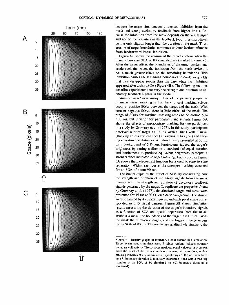
Figure 4 shows the results of three simulations that vary only in SOA. Figure 4A shows the creation and erosion of one row of boundary signals produced by a brief (15 ms, 30 fL) bar in a visual display with no subsequent stimulus. Brighter regions indicate higher cell activities, and the contour lines mark curves of equal activity. At stimulus onset (far left), the boundaries rapidly grow in strength and grow stronger as the excitatory bipole feedback develops. Shortly after stimulus offset, the boundaries drop in strength because of the lack of feedforward input from the visual image, and the boundaries erode from the contour ends toward the middle, as described earlier. The speed- ing up of erosion is evidenced by the inward bend to the outer contour line. A constant rate of erosion would produce a straight line.

Figure 4B shows the erosion of the same contour when onset of a pair of brief (15 ms, 30 fL) masking bars on either side of the target (4 pixel spaces of separation) follows the onset of the target by 5 simulated ms (marked by arrow). The activities of cells responding to the second stimulus have little effect


because the target simultaneously receives inhibition from the mask and strong excitatory feedback from higher levels. Be- cause the inhibition from the mask depends on the visual input and not on the activities in the feedback loop, it is short-lived, lasting only slightly longer than the duration of the mask. Thus, erosion of target boundaries continues without further influence from feedforward lateral inhibition.

Figure 4C shows the erosion of the target contour when the mask follows an SOA of 80 simulated ms (marked by arrow). After the target offset, the boundaries of the target weaken and erode such that when the inhibition from the mask arrives, it has a much greater effect on the remaining boundaries. This inhibition causes the remaining boundaries to erode so quickly that they disappear sooner than the case when the inhibition appeared after a short SOA (Figure 4B ). The following sections describe experiments that vary the strength and duration of excitatory feedback signals in the model.

Stimulus onset asynchrony. One of the primary properties of metacontrast masking is that the strongest masking effects occur at positive SOAs between the target and the mask. With zero or negative SOAs, there is little effect of the mask. The range of SOAs for maximal masking tends to be around 50- 100 ms, but it varies for participants and stimuli. Figure 5A shows the effects of metacontrast masking for one participant in a study by Growney et al. (1977). In this study, participants observed a brief target (a 16-ms vertical line) with a mask (flanking 16-ms vertical lines) at varying SOAs (At) and varying edge-to-edge distances. All stimuli were presented at 55 f L on a background of 5 ft-lam. Participants judged the target's brightness by setting a filter to a standard (of equal duration and luminance) to produce equivalent brightness percepts; a stronger filter indicated stronger masking. Each curve in Figure 5A shows the metacontrast function for a specific edge-to-edge separation. Within each curve, the strongest masking occurred for an SOA of about 90 ms.

The model explains the effect of SOA by considering how the strength and duration of inhibitory signals from the mask interact with the strength and duration of excitatory feedback signals generated by the target. To replicate the properties found by Growney et al. (1977), the simulated target and mask were presented for 15 ms at 30 fL on a dark background. The stimuli were separated by 4 - 8 pixel spaces, and each pixel space corre- sponded to 0.15 visual degrees. Figure 5B shows simulation results measuring the duration of the target's boundary signals as a function of SOA and spatial separation from the mask. Without a mask, the boundaries of the target last 135 ms. With the mask the duration changes, and the biggest change occurs for an SOA of 80 ms. The results are qualitatively similar to the

Figure 4. Density graphs of boundary signal erosion in a simulation. Target onset occurs at time zero. Brighter regions indicate stronger boundary cell activity. The contours mark out equal-value curves (arrows mark the onset of the mask): with no masking stimulus (A); with a masking stimulus at a stimulus onset asynchrony (SOA) of 5 simulated ms (B; boundary duration is relatively unaffected); and with a masking stimulus at an SOA of 80 simulated ms (C; boundary duration is shortened).

578 FRANCIS

A 1.4

1.2

09 r

0.8

--~ 0.6 iT 0.4

0.2

Separation RG ---o--1' / ~ - A - - 5'

~ 101 - ° - 3 0 / / \X

1° d z ~ ' k

-80 -40 0 40 80 120 160 200

A t (ms)

120

E ,- 125 O

a

~' 130 t -

O r n

135

Separation A - o - 0.60 ° [ % - . - 0.75 ° ~ \ - o - 0.90 ° / . ~ . - . - 1.06o ? , " ~ ,

I I I I

-50 0 50 100 150 A t (ms)

Figure 5. Masking is strongest for intermediate positive stimulus onset asynchronies (At). Paracontrast masking is weak. Masking falls off with distance. In A, Growney et al.'s (1977) psychophysical data. From "Metacontrast as a Function of Spatial Separation With Narrow Line Targets and Masks," by R. Growney, N. Weisstein, and S. Cox, 1977, Vision Research, 17, p. 1207. Copyright 1977 by Elsevier Science Ltd, The Boulevard, Langford Lane, Kidlington OX5 1GB, United Kingdom. Adapted with permission. In B, masking effects on duration of target signals in the model. Shorter durations correspond to stronger masking. Note that the y-axis runs in reverse. RG = participant's initials.

data in Figure 5A reported by Growney etal. ( 1977 ). Note that the y-axis runs in reverse because shorter boundary durations correspond to dimmer percepts.

Figure 5B shows that the model also has weak paracontrast masking (negative SOAs). This characteristic exists within the model because the feedforward inhibitory signals depend on the physical presence of the mask. When the mask precedes the target, the inhibition builds in strength and decays before generation of the target boundaries. As a result, the target signals remain relatively uninhibited, and paracontrast masking is weak. The weak paracontrast masking effects observed in Figure 5B occur because the inhibition from the mask can briefly delay the target boundaries from crossing a fixed threshold. Thus, the total duration of above threshold target signals is slightly shorter

when the mask precedes the target. This is not a strong effect because the excitatory signals produced by the target quickly overcome the inhibitory signals of the mask.

Target luminance. Weisstein (1972) varied the luminance of a target (filled circle) while fixing the mask (annulus) luminance at 16 fL. The target to mask luminance ratios could be 1.0, 0.5, 0.2, 0.0125, or 0.06125. Both stimuli were presented for 16 ms. Participants rated the brightness of each target against the percept of an unmasked stimulus of equal size and luminance. Figure 6A shows the resulting masking functions, for one participant, as SOA (At) varied. The key finding is that the shape of the masking function changed as target luminance decreased. In particular, strong masking occurred sooner for dimmer targets, and masking occurred at zero and negative SOAs for the dimmest targets. Two other participants showed qualitatively similar characteristics.

The model accounts for these findings because fainter targets generate weaker target boundaries and weaker excitatory feedback. As a result, the inhibition sent by the mask at even a short SOA is sufficient to shorten the duration of target signals. In the simulations, the target and mask durations were 16 ms, and the mask luminance was 16 fL. To produce the qualitative properties found by Weisstein (1972), it was necessary to reduce the luminance values of the simulated target to very small values (Figure 6B includes the target-mask ratios) because the on-center, off-surround cells in the model saturated at even small luminance values. A more accurate model of neural and LGN processing would help reduce the discrepancies between simulated and experimental stimulus values.

Because the data measured the relative strength of masking, the appropriate simulation measure is the change in boundary duration. Figure 6B plots changes in boundary duration from a no-mask condition. The model captures the key qualitative properties of the data. Decreasing the target luminance allows masking to occur for smaller and negative SOAs, and the strongest masking occurs for smaller SOAs as target luminance drops.

Target duration. Schiller (1965) varied target duration from 5-13 ms while fixing the mask duration at 100 ms. In this study the target was a black disk (reflectance of 9%) on a bright background (reflectance of 90%) that appeared in one of four locations on the visual display. The mask consisted of four annuli, of the same reflectance as the target, that surrounded the possible locations of the target. The participant's task was to identify the location of the target. Figure 7A plots the percentage of correct detections as a function of the ISI between target offset and mask onset. Separate curves are for fixed target durations. Detection percentages below 100 indicate metacontrast masking. The main finding is that performance improved as the duration of the target increases.

These results are consistent with the model hypothesis that the quality of the visual percept depends on the duration of boundary signals. Increasing the duration of the target increases the total amount of time the boundaries are present, which should lead to more accurate responses. In the simulations, the target was a bright ( 1 fL) bar of variable duration on a dark background, and the mask consisted of two flanking bars of the same luminance presented for 100 ms. Figure 7B plots the duration of boundaries from simulations that used the same


A f(AO

¢ -

" F _

.c_ ( I )

e -

e ' -

I 1.0

I

I I

I

I 0.125

I

0.5 , ,= /

0.06125

/ I I

-50 0

0.2

C !

180

At

dP

B

E t -

O

" ID

.__q

t ~

t - "

(3

| |

| |

| -I .i -10

-15

' o ' -50 0 5 100 At

At

L

150

At

Figure 6. The shape of the masking curve depends on the ratio of target and mask luminances. At small ratios (numbers above each curve), masking occurs for short stimulus onset asynchronies (At) and for paracontrast conditions. In A, Weisstein's (1972) psychophysical data. From "Metacontrast," by N. Weisstein, 1972, in D. Jameson and L. Hurvich (Eds.), Handbook of Sensory Physiology: Vol. 7. Visual Psychophysics (p. 263), Berlin, Germany: Springer-Verlag. Copyright 1972 by Springer-Verlag. Adapted with permission, In B, change in target boundary signal duration. Larger negative changes correspond to larger drops in brightness. JP = participant's initials,

target durations as in Schiller 's (1965) study. The results agree with the data. Increasing the duration of the target for a fixed ISI leads to longer durations of the boundaries, which implies better performance. As the ISI increases, boundary duration increases for each target duration. This latter result occurs, rather than a bow-shaped relationship, because the mask is of a long duration (100 ms) , which leads to monotonic metacontrast masking functions, as described below. The quantitative fit of

the model to the data is better if one assumes that there is a floor effect when the boundary duration is below 70 ms and a ceiling effect if the boundary duration is above 100 ms.

Feedforward Inhibition

This section considers a number of masking studies that vary the overall strength of feedforward inhibition. Any increase in

580 FRANCIS

• 70 ~! c~ 60 n

o ~" 50 ~ 0 E 4O

~o 30 • 5 ms

10

0 20 40 60 80

ISI (ms)

B 110

10o g " 90 ~ 80

"~ 70

0 m 60 50

n

- -0 - 9ms 7ms

i~ • 5 ms J I J I J ,,

0 20 40 60 80

ISI (ms)

Figure 7. Increasing target duration produces better detection of a target in a metacontrast display. In A, Schiller's (1965 ) psychophysical data. From "Metacontrast Interference as Determined by a Method of Comparisons," by P. Schiller, 1965, Perceptual and Motor Skills, 20, p. 282. Copyright 1965 by Southern Universities Press. Adapted with permission. In B, target boundary durations from model simulations. Longer durations correspond to better detection. ISI = interstimulus interval.

the overall strength of inhibition leads to stronger masking effects.

Distance. The data in Figure 5A from Growney et al. (1977) show that increasing the edge-to-edge separation of the target and mask produces weaker metacontrast masking. Mask- ing effects in this study disappeared by three degrees of separation. In the model the strength of feedforward lateral inhibition in the first competitive stage weakens with distance. With weaker inhibitory signals, the target signals last for a longer length of time. Thus, increasing separation between the target and the

mask results in weaker masking. Figure 5B shows that the model effects are qualitatively the same as the data in Figure 5A.

Mask duration. Increasing the duration of the masking stimulus produces stronger metacontrast masking. This finding is consistent with the model because longer lasting inhibition leads to faster erosion of target boundaries and shorter total duration of target boundaries. Two psychophysical studies support the properties of the model.

Breitmeyer (1978) showed that increasing the mask duration influenced the shape of the metacontrast curve. Figure 8A shows metacontrast masking curves, for 1 participant, for different mask durations. The target was a 16-ms disk, and the mask was a surrounding annulus of varying duration. Both stimuli were drawn with dark ink on a bright background of 20 fL. Partici- pants judged masking effects by matching the brightness of the target to a patch from a set of standard stimuli. Figure 8A shows two properties. First, masking effects grow stronger as mask duration increases. Second, the shape of the metacontrast masking function becomes closer to monotonic as mask duration increases.

The model also shows these trends, although there are quantitative differences. As the duration of the mask increases, so does the duration of the feedforward inhibitory signals sent from the mask to the target boundaries. This longer lasting inhibition speeds the erosion of target boundaries and shortens the overall duration of target boundaries. Thus, longer duration masks produce stronger metacontrast. Moreover, even at a short SOA, a long-duration mask inhibits the target's boundaries when they are strong as well as weak.

In the simulations, the target and mask were 30 f L bars on a dark background. The target was presented for 15 ms, and the mask duration varied from 1 - 128 ms in multiples of two. Figure 8B plots the duration of target boundary signals as a function of SOA and mask duration. Shorter target boundary durations correspond to stronger masking (the y-axis runs in reverse). The simulated results capture the key qualitative properties of Breitmeyer's (1978) data: As mask duration increases, masking strength increases and strong masking occurs at shorter SOAs.

In a related study, Di Lollo et al. (1993) showed that strong masking can occur at a zero SOA, if the mask duration is suffi- ciently long. Figure 9A shows psychophysical data for 2 participants. In this study, participants identified which edge of a (1 ms, 0.0681 cd-#s) target outline square had a missing piece. The mask was a surrounding outline square of equal brightness, with center pieces cut out (see Figure 9A) and was turned on simultaneously with the target. The mask duration was longer than the target duration by 0-160 ms. Percentage of correct identifications below 100 indicated masking effects. As Figure 9A demonstrates, performance worsened as the duration of the masking stimulus increased.

The model's explanation of this data is simple. When the target is present, its boundary signals receive two sources of excitation: from the target and from excitatory feedback. As a result, the mask's inhibition during simultaneous presentation with the target has little effect on the target's boundaries. When the target vanishes, its boundaries lose a source of excitation and start to erode. As mask duration increases, the erosion process is inhibited for a longer period of time, so the total duration of target


A 10

• 8

~ 6 e -

~ 4

BB

2

0

Mask Duration (ms) - -o -1

/ , . - " "- - , - 8 ~" ,~ ~ , " ~ ---n-- 16

t 7 ^ . " , . " - - ~

I I I

40 80 120 Stimulus Onset Asynehrony (ms)

B 100

110 C 0

Q 120

"10 t--

O

130

Mask Duration (ms)

I I I

0 40 80 120 Stimulus Onset Asynchrony (ms)

Figure 8. The shape of the masking curve depends on the duration of the mask. As the mask duration increases, stronger masking occurs at shorter stimulus onset asynchronies. In A, Breitmeyer's (1978) psychophysical data. From "Metacontrast Masking as a Function of Mask Energy," by B. Breitmeyer, 1978, Bulletin of the Psychonomic Society, 12, p. 51. Copyright 1978 by the Psychonomic Society. Adapted with permission. In B, target boundary durations from model simulations. Shorter durations correspond to stronger masking. Note that the y-axis runs in reverse. BB = participant's initials.

signals decreases. In the simulations, the target was 30 f L and presented for 15 ms on a dark background. The mask was of equal luminance and presented for an additional 5 -145 ms beyond the offset of the target. Figure 9B plots the duration of target boundary signals, with longer target boundary durations corresponding to higher percentages correct.

In both simulations, there are quantitative differences between the psychophysical and simulated data. Notably, the model requires substantially longer mask durations to produce monotone masking curves in Figure 8, and the model reaches a ceiling effect of mask duration sooner than the psychophysical data in Figure 9. Accounting for these differences requires elaborated simulations that consider the changes in stimulus type and partic-

ipant task with greater detail. Despite the differences, the overall influence of increasing mask duration is the same for both studies and simulations.

Contour. Sherrick and Dember (1970) demonstrated that the amount and spatial layout of mask contour affected masking strength. The target in their display was a brief ( 15 ms) black disk that appeared in one of two locations. Around each possible location a black masking stimulus (55 ms, ISI = 0) was also flashed. The participant's task was to identify the location of the target. The masks varied in two ways. A continuous mask was an annulus that had a single section removed. A distributed mask was an annulus with an equivalent amount of the contour removed but taken in several smaller sections rather than in one

582 FRANCIS

B

100

¢/) 90

( 0 t -

O 80 O3

(D n-

70

O 0 60 "6 ~ 50 ¢ -

~ 40

0.. 30

o MMH ~

L_' '_J I I I I

0 40 80 120 160

Duration of Mask Alone (ms)

130

g

"~ 120 "10 t - "-1 0 m "6 e- 110 0 . _

a

100

I

0 40 80 120 160

Duration of Mask Alone (ms)

Figure 9. Masking effects at zero stimulus onset asynchrony (SOA) as mask duration varies. Strong masking does occur at zero SOA if the mask is presented beyond target offset for a long-enough duration. In A, Di Lollo et al.'s (1993 ) psychophysical data. From "Stimulus-Onset Asynchrony Is Not Necessary for Motion Perception or Metacontrast Masking," by V. Di Lollo, W. Bischof, and P. Dixon, 1993, Psychologi- cal Science, 4, p. 262. Copyright 1993 by Cambridge University Press. Adapted with permission. In B, target boundary durations from model simulations. Shorter durations correspond to smaller percentages correct. VDL and MMH refer to the initials of the participants.

piece. The experiment also varied the amount of mask contour for both types of masks. Figure 10A plots the percentage of correct identifications, where less than 100 indicates masking. There are two main results f rom this study. First, masking de- pended on the amount of contour in the mask. Second, when two masks had equal contour, the distributed contour was more effective than the continuous contour. Gilden, MacDonald, and Lasaga (1988) found similar effects of contour amount with different stimuli across a broader range of ISis.

Figure 10B plots simulation results that account for this finding. In the simulations, the target was a br ief (15 ms) bright bar ( 1 f L ) on a dark background. The mask consisted of a pair of flanking bars (55 ms, ! f L ) presented after an ISI of zero. For the continuous mask, pixels at either end of each mask bar were set to the background luminance. For the distributed mask, pixels centered at one quarter and three quarters of the length of each mask bar were set to the background luminance. The target and mask stimuli were separated by 5 pixel spaces. Perfor- mance correct depends on the duration of target signals, so Figure 10B plots the duration of target signals against percentage of contour in the mask. The simulated results capture the two properties of the data: Masking increases with percentage

A too

80

O

60 D

15 .¢ 40

o~ 20

A

_ ' = _ . C°nt!;ut::

~ 0 . . . . . •

I I I I I

20 40 60 80 100 % Ring Contour

B 125

~ 12o

O0

'5 115

110

" ~ " ~ ¢ Continuous • ~ ~ ~a ~ ~ D i s t r t b u t e d

t I I I

20 80 40 60 % Contour

I

100

Figure 10. Masking effects grow stronger as percentage of masking contour increases. For masks with equal contour percentages, masking is stronger when the contour is distributed rather than continuously aligned. In A, psychophysical data is redrawn from Sherrick and Dember (1970). From "Completeness and Spatial Distribution of Mask Con- tours as Factors in Backward Visual Masking," by M. Sherrick and W. Dember, 1970, Journal of Experimental Psychology, 84, p. 180. Copy- right 1970 by the American Psychological Association. Adapted with permission of the author. In B, target boundary durations from model simulations. Longer durations correspond to better detection.


of contour, and the distributed contour provides stronger masking than the continuous contour.

The finding that masking strength depends on the amount of contour in the mask reflects the model property that the inhibition underlying metacontrast masking is generated by cells sensitive to mask contours. More contour leads to more cells responding and more inhibition. The finding that a distributed mask is more effective than a continuous mask of equal contour percentage reflects an interaction between the erosion process of the target stimulus and inhibition from the mask. As described earlier, the target boundary signals do not disappear uniformly but erode from contour ends to the contour middle. Also as described earlier, the inhibition from the mask is less effective if target boundaries have strong excitatory feedback supporting them. In the case of a continuous mask contour, the inhibitory signals generated by the mask are lumped together at the middle of the target contour. But the middle of the target contour receives the strongest excitatory feedback and so remains relatively unaffected by the mask. A distributed mask of the same contour percentage generates inhibition at the ends of the target contour. Because the end of the target contour receives weaker excitatory feedback, the inhibition has a strong effect and speeds the overall erosion of the target signals. Thus, the results in Figure 10 support the role of both excitatory feedback and lateral inhibition from contour-detecting cells in accounting for metacontrast masking.

It may be significant that the simulated stimuli differ substantially from the experimental stimuli. The differences may partly explain the discrepancies between experimental and simulated masking with the distributed mask. However, the model predicts that the main effect of distribution is robust enough to exist in bar stimuli as well as in the disk-annulus stimuli used by Sher- rick and Dember (1970).

Inhibitory Feedback

Although excitatory feedback causes persisting responses, inhibitory feedback has different influences on persisting responses and metacontrast masking. The following sections demonstrate that inhibitory feedback in the model accounts for properties of masking disinhibition.

Disinhibition I: Two masks. Given that the study of Sherrick and Dember (1970) showed that increasing the density of mask luminance edges produced stronger masking, it might be reason- able to suspect that if a display contained two masks, it would more strongly affect the target than a display with only one mask. A surprising result is that in some displays two masks result in weaker masking.

Figure 11A shows data from a study by Breitmeyer et al. (1981). The display consisted of a black disk target, T, presented for 15 ms on a bright background of 30 cd/m 2, a black annulus mask surrounding the disk, M~, of equal duration; and a second black annulus mask, M2, also of equal duration, that surrounded M~. In an initial experiment, T and M2 were presented simultaneously and followed by M~. Participants judged T by making brightness matches to a set of grey patches num- bered 1-10. The numerical difference between ratings of T with and without the mask or masks was taken as the strength of

masking. Breitmeyer et al. compared masking effects with and without M2 and calculated the difference as an indication of disinhibitory effects. Figure 11A shows, for 1 participant, that the presence of M2 reduced the strength of masking. The top curve with solid icons plots the masking magnitude against SOA for T and Ml alone and shows the typical inverted-U shape. The dashed line with open icons plots the masking magnitude with T, M~, and M2. The display with two masks has weaker masking. The bottom curve with cross icons plots the difference of the two masking curves and shows the strength of disinhibition.

The model's explanation of disinhibition requires understanding the role of inhibitory feedback in the BCS. Figure 1 refers to pathways of inhibitory feedback as spatial sharpening. In masking conditions, inhibitory feedback from the mask shortens the duration of persisting target boundaries. Feedback inhibition from a second mask around the first can weaken this feedback inhibition and thereby disinhibit the target.

For the simulations, the target and masks were presented for 15 ms at a luminance of 30 fL. The target and first mask were separated by 3 pixels, whereas the first and second mask (if present) were separated by 1 pixel. The target and second mask were presented simultaneously and followed by the first mask after a variable SOA. The top curves in Figure l i B plot the change in boundary signal duration of the target from a no- mask condition. The solid icons plot masking strength (change in target boundary duration) as a function of SOA when the display includes only the first mask. The open icons plot masking strength when the display includes both the first and second mask. The × icons plot the difference in target boundary duration for the two cases. In all cases the simulation results qualitatively match the data. The simulation results even capture the finding that the strongest disinhibition occurs for an intermediate SOA.

Disinhibition H: Stimulus onset asynchrony. With the same stimulus setup, Breitmeyer et al. (1981) showed that disinhibitory effects depend on the timing of the masks. They observed that disinhibition was strongest when the second mask, M2, preceded the normal metacontrast mask, M~. Figure 12A shows data from a study in which the SOA between Ml and T was fixed at 50 ms, whereas the SOA between T and M2 varied. The amount of disinhibition dropped quickly as M~ and M2 were presented simultaneously and went to zero when M2 followed Mi.

This result is consistent with the role of feedback inhibition in accounting for disinhibition. Because the inhibition is recurrent, the stimulus that first establishes itself in the network has an advantage over the following stimulus. Thus, when the second mask follows the first, inhibitory feedback from the first mask prevents the second mask from sending reciprocal inhibition to the first mask. This is a type of winner-take-aU network in which the winner, once it is established, has an advantage over new challengers.

The simulations used the same display parameters as before, but fixed the SOA between the target and Mj to be 60 ms. Figure 12B plots the disinhibition magnitude (recovery in target boundary duration) for variations in the onset of the target and M2. Like the data, disinhibition effects drop dramatically when MI and M2 are simultaneously onset, and M2 provides additional

584 FRANCIS

A

"10

t - O3

O3 t -

¢/) CO

0.4

0.2

-0.2

B B -- T - - o - - . T, M2

s - T

I I I I I I I

20 40 60 . 80 100 120 140

Stimulus Onset Asynchrony (ms)

B 40

~" 30

~ 20 ¢ -

v

o

-10

¢ T - - O - - • T , M 2

I I I I I I I

20 40 60 80 100 120 140

Stimulus Onset Asynchrony (ms)

Figure ll. Disinhibition effects with the presence of a second mask. Filled circles show the standard metacontrast masking curve for a target (T) and a mask (MI). Open circles show that the presence of a second mask (M2) results in less masking. The ×s show the disinhibition effect. In A, Breitmeyer et al.'s ( 1981 ) psychophysical data. From "Metacontrast Investigations of Sustained-Transient Channel Inhibitory Interactions," by B. Breitmeyer, M. Rudd, and K. Dunn, 1981, Journal of Experimental Psychology: Human Perception and Performance, 7, p. 773. Copyright 1981 by the American Psychological Association. Adapted with permission of the author. In B, simulated masking magnitude measured as changes in target boundary durations from a no-mask condition. BB = participant's initials.

masking (negative disinhibition) when M2 follows M~. Although the latter effect is weaker in the data than predicted by the model, it existed for all 3 participants in the Breitmeyer et al. (1981) study.

The model fails to account for one important property of these studies. Breitmeyer et al. (1981) also measured the masking influence of M2 on M1. They found that when M2 blocked the inhibition produced by M~, it did not mask the percept of Mj. In corresponding model simulations, the presence of/142 does shorten the boundaries of M~, contrary to the data. The model may be able to account for this finding with a different set of

parameters, but further studies (both psychophysical and simulated) are necessary to sort out these details. For the model to account for this finding, M2 would need to more strongly weaken the Mt inhibitory feedback than the MI self-excitatory feedback.

Disinhibition I11: Distance. Finally, Breitmeyer et al. (1981) showed that disinhibition occurs over a spatial range that is more narrow than the spatial range of metacontrast masking. They varied the stimulus display in two ways. First, they presented M2 continuously throughout the display. They made this modification because a long-duration second mask would more strongly activate sustained channels, which they thought


A 0.4

-~ 0.2 ¢-

¢ -

o 0 .-g_

.~_

.co E3

-0.2

BB

I I I I I I I

-180 -120 -60 0 60 120 180

T - M 2 Onset Asynchrony (ms)

B

E v ¢)

"o 5

c 0 )

= 0 ._o -g ..c c

10

I

-180 I I I I I

-120 -60 0 60 120 180

T - M 2 O n s e t A s y n c h r o n y (ms)

Figure 12. Disinhibition effects as a function of the stimulus onset asynchrony between the target (T) and the second mask (M2). Disinhibition occurs only when the second mask precedes the first mask. When the second mask follows the first mask, stronger masking (negative disinhibition) occurs. In A, Breitmeyer et al.'s (1981) psychophysical data. From "Metacontrast Investigations of Sustained-Transient Channel Inhibitory Interactions," by B. Breitmeyer, M. Rudd, and K. Dunn, 1981, Journal of Experimental Psychol- ogy: Human Perception and Performance, 7, p. 774. Copyright 1981 by the American Psychological Association. Adapted with permission of the author. In B, disinhibition effects from model simulations. BB = participant's initials.

were responsible for disinhibition. Second, they systematically varied the edge-to-edge separation between M1 and M2. Disinhi- bition effects dropped dramatically as the separation between M~ and M2 increased. Figure 13A plots the disinhibition magnitude as a function of spatial separation between the masks for 1 participant.

The limited spatial range of disinhibition is consistent with the model because the spatial range of inhibitory feedback is quite small. In the simulations, the second mask was presented 1 s before the onset of the target and remained on throughout

the display. The SOA between the target and the first mask was 50 ms. The masks were separated by 1 - 6 pixels, and the target and first mask were separated by 3 pixels. Disinhibition magnitude was measured by comparing changes in target durations with the first mask alone and with both masks. Figure 13B plots the disinhibition magnitude as a function of spatial separation between the masks. Disinhibition magnitude drops off rapidly as the two masks are separated, indicating the limited spatial range of inhibitory feedback. The model predicts a slight increase in masking (negative disinhibition) for a spatial separa-

586 FRANCIS

A

19 "O - i

t - O }

0.6

0.4

0.2

-0.2

BB

+

\

T - M1 S O A -t- 45 ms x 65 ms

- ~ _ _ - - ~

I I I I I

0 17 34 51 68

M 1 - M 2 Spat ia l S e p a r a t i o n (rain)

B

4

g I1)

" O --, 2 t - o ) t~

0

-2

T - M 1 S O A x 50 ms

I I I I I

0 17 34 51 68

M1 " M2 Spatial Separation (min)

Figure 13. Disinhibition effects as a function of the spatial separation between the second mask (M2) and the first mask (M1). Disinhibition occurs only when the masks are very close. In A, Breitmeyer et al.'s ( 1981 ) psychophysical data. From "Metacontrast Investigations of Sus- tained-Transient Channel Inhibitory Interactions," by B. Breitmeyer, M. Rudd, and K. Dunn, 1981, Journal of Experimental Psychology: Human Perception and Performance, 7, p. 776. Copyright 1981 by the American Psychological Association. Adapted with permission of the author. In B, disinhibition effects from model simulations. BB = participant's initials; T = target; SOA = stimulus onset asynchrony.

tion of 21 min, which is inconsistent with the data. This discrep- ancy might be resolved by changes in the model parameters. This has not been rigorously explored, however, as the qualitative fit to the data is otherwise quite good.

Feedforward inhibition from the second mask to the target was weak because the inhibition follows the model stage of transmitter habituation described in Boundary Contour System Dynamics. By the time of the target's onset, the second mask had depleted transmitter amounts so that the inhibitory signals

were too weak to have much effect on the duration of the target's signals. The habituative transmitters play a more important role in explaining data on visual persistence, temporal integration, and apparent motion. They also contribute to a prediction described in Habituation later in this article.

S t imulus Onse t A s y n c h r o n y Versus In ters t imulus Interval

Masking curves generally plot the strength of masking against SOA. Although the previous simulation results were plotted in the same manner to facilitate comparisons with experimental data, additional properties of the model are revealed by plotting masking strength against ISI. Figure 14 plots masking functions (change in boundary duration from no-mask to mask conditions) for 25-, 50-, 75-, 100-, and 125-ms target durations for two mask durations. Figures 14A and B plot the masking strength against SOA, whereas Figures 14C and D plot the same data against ISI. When plotted against SOA, it is apparent that the short-duration targets receive the most masking at the shorter SOAs and the long-duration targets receive stronger masking at the later SOAs. This is particularly true for the long-duration mask ( 100 ms) , but also holds true for the short-duration mask (25 ms). Masking is weak in the model for short SOAs with long-duration targets because much of the display consists of the target and mask presented together. Because there is no erosion of target boundary signals when the target is part of the display, the mask inhibition has little effect.

On the other hand, when the same simulated data are plotted against ISI, the masking curves for different target durations are nearly superimposed. The superposition reflects that model masking occurs when the mask is presented while the target boundaries start to erode. When the mask has a long duration (Figure 14C), it is most effective if it starts to send inhibition as soon as target boundaries erode and continues to send inhibition throughout the erosion process. When the mask has a short duration (Figure 14D), it is most effective if it waits until the target boundaries have eroded somewhat (positive ISI) and then sends its inhibition to briefly speed the rate of erosion. None of these properties strongly depend on the target duration, as long as target duration and luminance are large enough to produce strong resonance in the BCS. The model does predict a small effect of target duration, with shorter target durations demon- strating larger masking. This effect may change with adjustments in model parameters, and so it is not a strong prediction of the model.

At first glance this model property appears to be in conflict with experimental data. Kahneman (1967) showed that variations in the durations of the target and mask had little effect on the strength of metacontrast masking if masking strength was plotted against SOA. As SOA varied, the curves for different durations overlapped almost perfectly (Figure 15A). Given these strong results, Kahneman proposed an onset-onset law, which is now frequently referred to as the SOA law, as a funda- mental property of metacontrast masking.

However, there are some problems with Kahneman's study. Kahneman (1967) varied the target and mask durations together. The SOA law does not hold when the target and mask have


A

~ - 3 0

~ -20

nn c_ "~ -10

! i I

I I •

I I 50 100

Target duration I -o- 25 ms [

om: I ' ~ "&- 100 ms I

' , \ ' , , \ I

SOA (ms)

B ~E "15

f,

CI -10

m

- -5

g

0

Target duration I \ - o - 25 ms r \ e ~ i ~ -e- 50ms

j ~ , / \ , / \ ~ 7sins / ;~ le~ ~J \ -A- 10o ms

I / V 7/A :i A ', \

0 50 100 150 200 250 SOA (ms)

C [ n ~ Target duraUon] D I "s . ~ -o- 25 ms I I ~ . ,~ -~ ÷ 50m~ I ~" -ls

g / p" " ~ -~- looms I 8

.1o -20 ~

e - e -

"k -,o "k

0 0

-100 -50 0 50 100 150 200 -10O -50 0 ISI (ms)

I Target duration - o - 25 ms -e- 50 ms -~ - 75 ms -&- 1 0 0 m s - m - 125 ms

50 100 150 200 ISI (ms)

Figure 14. Change in target boundary duration as a function of interstimulus interval (ISI) or stimulus onset asynchrony (SOA) for various target durations and two mask durations. In A, change in target boundary duration as a function of SOA for a mask duration of 100 ms and various target durations. The model predicts that strong masking (large negative values) occurs at shorter SOAs for short target durations. In B, same as in A except mask duration is 25 ms. The results are qualitatively similar to A, except each curve shows an inverted-U function of masking. In C, a replotting of the data in A (mask duration = 100 ms) shows that the data obey a strong ISI law. In D, a replotting of the data in B (mask duration = 25 ms) also shows a strong ISI law.

different energies (Figures 6 and 8). Moreover, there is some question about the law's validity for equal energy stimuli. Weisstein and Growney (1969) attempted to replicate Kahne- man's results. They found a reliable effect of stimulus duration. Figure 15B plots the data from their first experiment (which most closely matched the display parameters used by Kahne- man). In the data, the strongest masking effects occurred with the shortest stimulus durations.

Significantly, Weisstein and Growney (1969) found results more similar to Kahneman's (1967) for subsequent experiments. Some (of the 5 total) participants participated in more than one experiment, and the trend across experiments suggests that participants learned to ignore the effects of target duration. This is a plausible explanation because in both studies participants rated the strength of metacontrast masking by simply noting how faint the target appeared, rather than directly comparing

588 FRANCIS

A

e- 3

rr e-

• 2

Duration B 5 - - o - - 25 ms - • - 5 0 m s

7 5 m s 4 - & - 1 0 0 m s

S

3

¢r 2

1

i i F I I 0

50 100 150 200 250

SOA (ms)

Duration - - o - - 25 ms - o - 50 ms --12-- 125 ms

i i i i 1

0 50 100 150 200 250

SOA (ms)

C -50 Duration D 80

E "-" -40 t-- .o_

£3 -30

'1o e-, "~ -20 o m .~_

~ -10 e-

t -

O

F 1 I

0 50 100

- - o - - 25 ms - • - 5 0 m s

75 ms - & - 1 0 0 m s

--13-- 125 ms

150 200 250

SOA (ms)

100

~ " 120 E ' - 140 O

-~ 160 a

0~ 180 t-"

"1

o 200

220

240

Duration - - o - - 25 ms - - • - 50 ms - - ~ - - 75 ms

A,., 100 ms

50 100 150 200 250

SOA (ms)

Figure 15. Metacontrast masking as a function of stimulus onset asynchrony (SOA) when target and mask durations increase together. In A, psychophysical data from Kahneman (1967) suggest that stimulus duration is unimportant and that masking strength depends solely on SOA. From "An Onset-Onset Law for One Case of Apparent Motion and Metacontrast," by D. Kahneman, 1967, Perception & Psychophysics, 2, p. 579. Copyright 1967 by the Psychonomic Society. Adapted with permission. In B, psychophysical data from Weisstein and Growney (1969) failed to replicate Kahneman's findings. Instead, they show that increases in stimulus duration lead to weaker masking. From "Apparent Movement and Metacontrast: A Note on Kahneman's Formulation," by N. Weisstein and R. Growney, 1969, Perception & Psychophysics, 5, p. 326. Copyright 1969 by the Psychonomic Society. Adapted with permission. In C, data from model simulations when the change in target boundaries is plotted against SOA. Large negative changes indicate strong masking. At short SOAs the masking strength follows a strong SOA law as in A. The model fails to obey the SOA law for longer SOAs. In D, data from model simulations when the total duration of target boundaries is plotted against SOA. Shorter durations indicate stronger masking. Note that the y-axis runs in reverse. The data match the findings in B.


the target to an unmasked standard stimulus. Following Bloch's law (or the Bunsen-Roscoe law), a 25-ms target should look fainter than a 125-ms target, even if neither is being masked. It may have been difficult for naive participants to disentangle these effects. Weisstein and Growney's participants may have initially confused the effects of Bloch's law with masking (thus leading to stronger masking for shorter targets) but learned to distinguish the effects with experience. Kahneman's participants may also have experienced similar problems early in the experiment.

Both Kahneman's (1967) and Weisstein and Growney's (1969) experimental data at longer SOAs seems to be incompati- ble with related experimental data. Although Figures 15A and B show strong masking with an SOA of 250 ms, few studies find evidence of masking at SOAs beyond 150 ms (see Figures 5, 8, and 11 ). It may be that the method used to investigate the SOA law is an unreliable measure of masking.

Although the model generally obeys an ISI law rather than an SOA law, it is still able to explain some aspects of Kahne- man's (1967) data. Suppose that (at least at short SOAs) the participants in Kahneman' s study were able to adequately judge the strength of metacontrast masking without confusion of Bloch's law. Then the corresponding model measure would be the change in target boundary duration in the masking condition compared to the no-mask condition. Figure 15C plots the change in target boundary duration for various target and mask durations as a function of SOA. As in Kahneman's study, the target and mask durations vary together. The simulated data show a strong SOA law at short SOAs but not at long SOAs. For the model, this property exists because masking strength depends partly on how long the mask is present after offset of the target. When the target and mask have the same duration and when they are presented simultaneously for at least part of the display, the duration of the mask presented by itself exactly equals the SOA. This property holds in Kahneman's data (Figure 15A) for short SOAs, and it is here that his curves are most similar. Thus, the SOA law found by Kahneman is coincidental; it requires that the target and mask have identical durations and short SOAs.

If it is supposed that participants in Weisstein and Growney (1969) could not distinguish effects of masking from effects of Bloch's law, then the corresponding measure in the model is the total duration of target boundary signals rather than changes in boundary duration. The data, plotted in Figure 15B, show that increasing target and mask durations lead to weaker masking. Figure 15D plots the total duration of target signals from the simulations. The resulting curves are quite similar to the data found by Weisstein and Growney. Thus, by considering participants' interpretation, the model partly accounts for both sets of data. Additional psychophysical experiments, with proper anchoring, are needed to verify the model's account of these data and its prediction of an ISI law.

Predictions

Besides accounting for known properties of metacontrast masking, the model makes a number of predictions that test the model components. This section describes some of these predictions.

Spatial Range of Inhibitory Feedback

The strong recurrent inhibition responsible for disinhibition effects has a shorter spatial range than the feedforward inhibition responsible for many metacontrast properties. Thus, the model predicts that metacontrast masking cannot be disinhibited unless the mask and target are very close together. When the mask and target are farther apart, metacontrast masking may occur but disinhibition cannot.

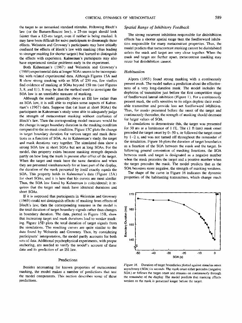
Habituation

Alpern (1953) found strong masking with a continuously present mask. The model makes a prediction about the effectiveness of a very long-duration mask. The model includes the depletion of transmitter just before the first competitive stage of feedforward lateral inhibition (Figure 1 ). For a continuously present mask, the cells sensitive to its edges deplete their available transmitter and provide less net feedforward inhibition. Thus, for masks presented before the onset of the target and continuously thereafter, the strength of masking should decrease for larger values of SOA.

In simulations to demonstrate this, the target was presented for 50 ms at a luminance of 1 fL. The (1 ft-lam) mask onset preceded the target onset by 0 -50 s, or followed the target onset by 1-2 s, and was not tumed off throughout the remainder of the simulation. Figure 16 plots the duration of target boundaries as a function of the SOA between the mask and the target. In following general convention of masking functions, the SOA between mask and target is designated as a negative number when the mask precedes the target and a positive number when the target precedes the mask. The model predicts that as the SOA becomes more negative, the strength of masking weakens.

The shape of the curve in Figure 16 indicates the dynamic properties of the habituating transmitters, which change much

170

E 160

Q

~, 150

140

w

I I i I I I

-50 -40 -30 -20 -10 0 SOA (s)

Figure 16. Duration of target boundaries plotted against stimulus onset asynchrony (SOA) in seconds. The mask onset either precedes (negative SOA) or follows the target onset and remains on continuously through the remainder of the display. The model predicts that masking effects weaken as the mask is presented longer before the target.

590 FRANCIS

slower than cell activities. For larger negative values of SOA, the transmitters have more time to habituate and therefore produce weaker inhibition and less masking. Masking effects do not entirely disappear even for an SOA of - 5 0 s because the transmitter amount equilibrates at a non-zero level after about 50 s.

Neurophysiological Analogues

The BCS model is not solely a computational model, its mechanisms are hypothesized to exist in cortical analogues of visual cortex. In particular, the feedforward lateral inhibition responsible for metacontrast masking corresponds to the inhibition involved in creating endstopped hypercomplex cells. End- stopped cells studied by Orban et al. (1979b) had an average spatial range of 1.9 °, which is large enough to account for the lateral inhibition in metacontrast. Additional research suggests that endstopped cells are built from combinations of nonend- stopped cells. Bolz and Gilbert (1986), for example, show that reversibly inactivating Layer 6 in the cat reduces or abolishes endstopping in the superficial layers. These properties are consistent with the first competitive stage in the BCS architecture. Moreover, the BCS's explanation of metacontrast data suggests that inactivation of Layer 6 should destroy the masking effects of adjacent stimuli.

studies need to show how the duration of BCS signals quantita- tively affects the measures of brightness, recognition, and detection used in experimental masking studies. Applying such map- pings to the current simulations would add complexity and might hide some of the model properties. Also, limitations in calculation speed must be overcome to allow larger simulations with more realistic stimuli.

The fact that the model can account for a variety of metacontrast data despite these limitations leads to some strong predictions. The model predicts that the experimental results discussed in this article are robust properties of masking that are not restricted to particular methodologies or stimuli. This provides an easy test of the model's explanation of the data sets discussed here. Perhaps the best evidence that the model strikes a good balance between being overly specific or overly general is that it produces testable predictions. Experimental studies can test the model at the same level analysis that it uses to account for data.

Although it is clear that much work remains, it is significant to recognize that no other account of metacontrast masking covers all of the data sets discussed here. Moreover, the closest competitor, transient-sustained theory, has not been quantified in sufficient detail to allow the level of analysis applied to the BCS model.

Fitting Data and Model Extensions

Sometimes a model that provides a precise fit to one data set is fundamentally unable to account for even the general trends of a related data set. This article demonstrates that the BCS model provides a broad fit of many metacontrast data. The simulations reported here generally focus on capturing strong trends in the metacontrast data rather than accounting for every bump and curve. For example, increasing mask duration has a stronger effect in the study of Breitmeyer (1978) than in the study of Di Lollo et al. (1993). Because the two studies use different participants, methods, and stimuli, it is not surprising that they show different effects of mask duration. Although the model correctly shows that increasing mask duration produces stronger masking, it does not identify the effects of changing participants, methods, or stimuli. Similar comments apply to the effects of target luminance (Figure 6), distributed contours (Figure 10), and disinhibition (Figure 12). Here, the model exhibits the basic properties of each effect, but fails to quantita- tively fit the data very well. The only recourse is to hope that future refinements of the model will account for these details.

Significantly, the model is in a good position to account for these details. The general characteristics of metacontrast masking are explained by general characteristics of the BCS model. Explaining the more specific details of each experimental condition requires identifying the spatial and temporal properties of individual cells in the model. Thus, general experimental data is accounted for with general model properties, and details of the experimental data are addressed with details of the model.

In addition to accounting for experimental details, the model needs to be extended in several ways. For example, the current simulations compare the duration of BCS signals across conditions to demonstrate the effect of metacontrast masking, Future

Discussion

This article describes how mechanisms of excitatory feedback, inhibitory feedback, and feedforward inhibition in a neural model of visual perception account for complicated dynamic data from metacontrast masking studies. The literature on metacontrast masking is large, and current research is exploring the model's ability to account for additional experimental data. Ta- ble 1 summarizes the role of the different mechanisms in accounting for the data discussed here.

It is not the case that any network with these mechanisms accounts for the data. For example, Wilson and Cowan (1973) simulated masking in a neural network model with recurrent excitation and inhibition but were unable to demonstrate the effect of SOA. Other studies of visual perception place constraints on the receptive fields and connections between individual cells. Indeed, Grossberg and Mingolla (1985a, 1985b) designed the BCS network to account for spatial properties of visual perception. This suggests that metacontrast masking should not be investigated independently of other aspects of visual perception because many spatial and temporal properties of visual perception are closely linked.

Indeed, the same few mechanisms explain related properties of dynamic vision as measured through studies of visual persistence, temporal integration, apparent motion, and cortical afterimages. The BCS model is thus unifying diverse psychophysical data on dynamic vision, and no other model of dynamic vision accounts for all of these data sets. Beyond the dynamic properties of vision discussed here, the BCS mechanisms have also been shown to be consistent with a large set of spatial characteristics. The dynamic emergent properties used to explain metacontrast masking are consistent with, and depend upon, the BCS's roles in boundary completion, texture segrega-


Table 1 Summary of Mechanisms Involved in the Model's Account of Psychophysical Data and Predictions

Model mechanism

Resonance Feed forward Inhibitory Experimental result strength inhibition feedback Habituation

Data SOA Target luminance ¢" Target duration ¢" Distance Mask duration Contour ~" Disinhibition Disinhibition: SOA Disinhibition: Distance

Predictions ISI law ¢" Continuous mask Disinhibition distance

¢-

¢.

¢-

Note. SOA = stimulus onset asynchrony; ¢" = variations in the variable of interest primarily affect the corresponding mechanism; ISI = interstimulus interval.

tion, shape from shading, brightness perception, 3-D vision, and motion processing, among others. Thus, the theory explains not only how metacontrast masking occurs but also why.

Significantly, the model accounts for all of these data sets in a robust fashion. All of the simulations reported here used a single set of parameters. The changes in network behavior depend only on the corresponding changes made in the simulated display. Small changes in any of the parameters would not dramatically change the qualitative behavior of the network, although there would be quantitative differences. Most of the parameters used here are the same as those used in Francis et al. (1994), Francis and Grossberg (1996a, 1996b) and Francis ( 1996a, 1996b), with the few changes providing the model with new properties that do not negate previous explanations. This type of robustness is critical because it allows the model to retain desirable characteristics even as new data constrain it. This does not mean, however, that the model cannot be tested. To the contrary the model makes testable predictions that are now being investigated.

The model 's explanation of metacontrast data is fundamentally different from the theory of transient-sustained inhibition (Breitmeyer, 1984). Given the success of the BCS at explaining these data sets, the challenge is now to proponents of the transient-sustained theory to show equivalent results. Such results may be hard to come by. Although the core of the transient- sustained theory is simple: Time-lag differences explain why maximal masking occurs for intermediate SOAs. From that core idea, the theory has grown much more complicated. For example, Breitmeyer (1978) argued that sustained cells inhibit sustained cells. Breitmeyer et al. ( 1981 ) argued that sustained cells inhibit transient cells and that transient cells inhibit transient cells. Thus, in the modified transient-sustained theory, everything inhibits everything else, and it becomes unclear whether all these inhibitory signals can be balanced to allow perception

to occur at all. This article shows that a neural network model with recurrent excitation and inhibition does not need the time lags and complex inhibitory interactions of the transient-sustained theory.

These findings emphasize an important point for models of visual perception. Network interactions between thousands of individual cells can lead to fundamentally different behavior than would be expected from an analysis of an individual cel l 's temporal or receptive field characteristics. In the BCS model, the properties of metacontrast masking emerge from the interactions of resonating signals and inhibition rather than being built into any individual cell. To understand human vision, one must understand its mechanisms, and this means understanding the emergent behavior of large sets of cortical neurons. Despite the daunting complexity of the network if investigated cell by cell, this study demonstrates that a few key mechanisms govern its dynamic behavior and that the network behavior matches psychophysical data.

Re fe rences

Alpem, M. (1953). Metacontrast. Journal of the Optical Society of America, 43, 648-657.

Bolz, J., & Gilbert, C. (1986). Generation of end-inhibition in the visual cortex via interlaminar connections. Nature, 320, 362-365.

Breitmeyer, B. (1978). Metacontrast masking as a function of mask energy. Bulletin of the Psychonomic Society, 12, 50-52.

Breitmeyer, B. (1984). Visual masking: An integrative approach. New York: Oxford University Press.

Breitmeyer, B., & Ganz, L. (1976). Implications of sustained and transient channels for theories of visual pattern masking, saccadic suppres- sion, and information processing. Psychological Review, 83, 1-36.

Breitmeyer, B., Rudd, M., & Dunn, K. (1981). Metacontrast investigations of sustained-transient channel inhibitory interactions. Journal of Experimental Psychology: Human Perception and Performance, 7, 770-779.

592 FRANCIS

Busey, T., & Lotus, G. (1994). Sensory and cognitive components of visual information acquisition. Psychological Review, 101, 446-469.

Chen, S., Bedell, H., & O~men, H. (1995). A target in real motion appears blurred in the absence of other proximal moving targets. Vision Research, 35, 2315-2328.

Di Lollo, V., Bischof, W., & Dixon, P. (1993). Stimulus-onset asynchrony is not necessary for motion perception or metacontrast masking. Psychological Science, 4, 260-263.

Francis, G. (1996a). Cortical dynamics of lateral inhibition: Visual persistence and ISI. Perception & Psychophysics, 58, 1103-1109.

Francis, G. (1996b). Cortical dynamics of visual persistence and temporal integration. Perception & Psychophysics, 58, 1203-1212.

Francis, G., & Grossberg, S. (1996a). Cortical dynamics of boundary segmentation and reset: Persistence of residual traces and orientational aftereffects. Perception, 25, 543-567.

Francis, G., & Grossberg, S. (1996b). Cortical dynamics of form and motion integration: Persistence, apparent motion, and illusory contours. Vision Research, 36, 149-174.

Francis, G., Grossberg, S., & Mingolla, E. (1994). Cortical dynamics of feature binding and reset: Control of visual persistence. Vision Research, 34, 1089-1104.

Gilden, D., MacDonald, K., & Lasaga, M. (1988 ). Masking with mini- mal contours: Selective inhibition with low spatial frequencies. Per- ception & Psychophysics, 44, 127-132.

Grossberg, S. (1994). 3-D vision and figure-ground separation by visual cortex. Perception & Psychophysics, 55, 48-120.

Grossberg, S., & Mingolla, E. (1985a). Neural dynamics of form perception: Boundary completion, illusory figures, and neon color spreading. Psychological Review, 92, 173-211.

Grossberg, S., & Mingolla, E. (1985b). Neural dynamics of perceptual grouping : Textures, boundaries, and emergent segmentations. Percep- tion & Psychophysics, 38, 141-171.

Grossberg, S., & Todorovi6, D. (1988). Neural dynamics of 1-D and 2-D brightness perception: A unified model of classical and recent phenomena. Perception & Psychophysics, 43, 241-277.

Growney, R., Weisstein, N., & Cox, S. (1977). Metacontrast as a func-

tion of spatial separation with narrow line targets and masks. Vision Research, 17, 1205-1201.

Hubel, D., & Wiesel, T. ( 1965 ). Receptive fields and functional architecture in two nonstriate visual areas (18 and 19) of the cat. Journal of Neurophysiology, 28, 229-289.

Kahneman, D. (1967). An onset-onset law for one case of apparent motion and metacontrast. Perception & Psychophysics, 2. 577-584.

Ludtke, D. (1992). NXPlot3d (Version 3.0) [Computer software]. Houston, TX: Rice University, Department of Physics. Available www.url:http://ion.rice.edu/nsci/plotting/nxplot3d.html

Matin, E. ( 1975 ). The two-transient (masking) paradigm. Psychological Review, 82, 451-461.

0~men, H. ( 1993 ). A neural theory of retino-cortical dynamics. Neural Networks, 6, 245-273.

Orban, G., Kato, H., & Bishop, P. (1979a). Dimensions and properties of end-zone inhibitory areas in receptive fields of hypercomplex ceils in cat striate cortex. Journal of Neurophysiology, 42, 833-849.

Orban, G., Kato, H., & Bishop, P. (1979b). End-zone region in receptive fields of hypercomplex and other striate neurons in the cat. Journal of Neurophysiology, 42, 818- 832.

Schiller, P. ( 1965 ). Metacontrast interference as determined by a method of comparisons. Perceptual and Motor Skills, 20, 279-285.

Sherrick, M., & Dember, W. (1970). Completeness and spatial distribution of mask contours as factors in backward visual masking. Journal of Experimental Psychology, 84, 179-180.

Von der Heydt, R., Peterhans, E., & Baumgartner, G. (1984). Illusory contours and cortical neuron responses. Science, 224, 1260-1262.

Weisstein, N. (1972). Metacontrast. In D. Jameson & L. Hurvich (Eds.), Handbook of sensory physiology: Vol. 7. Visual psychophysics (pp. 233-272). Berlin, Germany: Springer-Verlag.

Weisstein, N., & Growney, R. (1969). Apparent movement and metacontrast: A note on Kahneman's formulation. Perception & Psychophys- ics, 5, 321-328.

Weisstein, N., Ozog, G., & Szoc, R. (1975). A comparison and elabora- tion of two models of metacontrast. Psychological Review, 82, 325- 343.

Wilson, H., & Cowan, J. (1973). A mathematical theory of the functional dynamics of cortical and thalamic nervous tissue. Kybernetik, 13, 55-80.

Appendix

Simulation Details

Network Equations where Ipq is the retinal luminance at position (p, q), A is the maximum activity of the cell, - C is the minimum activity of the cell, and

Level O: Image Plane

Each pixel has a value associated with retinal luminance. The pixel- luminance values of the different stimuli are described in the text.

Level 1: Center-Surround Cells

The activity X ]j of a Level 1 cell centered at position (i, j ) obeys a shunting on-center, off-surround equation

d X " _ - - - - X ~ + (A - X 3) • Boeqleq - (X li + C) ~, DijpqCq, (A1)

dt Pq Pq

Bqe q = B e x p [ - o t -2 log 2[( i - p)2 + ( j _ q)2]] (A2)

D,jpq = D exp [ - / 3 -2 log 2[( i - p)2 + ( j _ q)2]] (A3)

are excitatory and inhibitory Gaussian weighting functions, respectively. The term log 2 means the parameters a and /3 set the radius of their respective Gaussians at half strength. Parameters B and D are constant scaling terms. In the current simulations, the kernels play a minor role, as the range of calculations is limited to the center pixel of the kernels.

To save computation, the equilibrium response of the differential equation is found by setting the left hand side of Equation A1 equal to zero. The resulting algebraic equation can be solved to find


A E Bijpqlpq - C E Dotal m J - - I ~ g q X o - (A4)

1.0 + Y, (Bop ~ + Dop,)l ~ Pq

Leve l 2: Or i en t ed S imple Cel ls

The following equations define oriented simple cells that are centered at position (i, j ) with preferred orientation k. To create a vertically oriented input field, or infield, that is specific to the polarity of the luminance gradient, divide an elongated region into a left half L0, and a right half R0k. Add up the weighted sum of the Level 1 inputs within the range of the left side

F , j , = Z E,a, qX~q (A5) pq E L,jk

and the right side

Gok = Y. EopqX ' m (A6) pq E R,jl~

of the region, with

Eijeq = e x p [ - y 2 log 2(i - p)2]; (A7)

decreasing for inputs further away from the oriented centerline of the infield, where the parameter y controls the rate of falloff. Then a simple cell that is selectively responsive to a bright-to-dark luminance gradient obeys the differential equation

dX 2~o iJk 2 BD dt - X ok + [Fiyk -- Gok]+' (A8)

where [p] + = max(p, 0). A cell responsive to a dark-to-bright luminance gradient obeys the equation

dX 2DB ijk -- X 2DB + [Gijk -- F0,] + . (A9)

dt

To save computation, the activities of these cells were computed at equilibrium as

X ~ff ' = [Fuk -- Go,] +, (AIO)

and

X ~o = [Gvk - F0k] +. (AI 1 )

d X 4 dt °k = K[L(M - X~k) - (X3k + j )X4k] . (n13)

This equation says that the amount of available transmitter X 4k accumu- lates to the level M, using term K L ( M - X ~k), and is inactivated by mass action at rate K ( X 3k + J )X 4k, where J is the tonic input of a gated dipole and X 3, is its phasic increment. The rate K is set much smaller than 1.0 so that these equations operate on a slower time scale than the equations describing cell activities. At the beginning of each simulation, each transmitter value is set to the nonstimulated equilibrium value X 4k = L M / ( L + J).

Leve l 5: F irs t Compet i t i ve S tage o f H y p e r c o m p l e x Cells

The gated signals of a fixed orientation compete using on-center, off- surround spatial interactions. Along with the tonic signal coming up through the habituative transmitters, each cell also receives a tonic input that supports disinhibitory activations at the next competitive stage (see Grossberg & Mingolla, 1985a, 1985b). The activity of a Level 5 cell obeys the differential equation

dX 3k _ 5 dt - - X o , + J + (X3k + j ) X 4 ,

_ X 5 3 4 tjk Y~ Por~(X pqk "~ J ) X pqk, (A14) Pq

where - X 3k models passive decay, the parameter J establishes a nonzero baseline of activity for the cell. the term (X 3.k + J )X 4k is the gated excitatory input from the lower level at the same position and orientation, and the term

X5k Z PiJpq(X3pqk ~" j ) X 4 q k

pq

is the inhibitory input from the lower level cells of the same orientation and nearby spatial positions. The inhibitory weights fall off in strength as the spatial distance between cells increases, as in

e q p q = P e x p [ - 6 -2 log 2[( i - p)Z + ( j _ q)2]], (A15)

where P scales the strength of the inhibition, and 6 controls the spread. For the simulations in this article, the differential equation Was solved

at equilibrium as

J + ( X 3 k + J ) X 4 ijk (A16) X 5

qk = 1 . 0 + ]~ ei)pq(X3ntk + J ) x4pqk " pq

Leve l 3: Or ien ted C o m p l e x Cells

Each cell in Level 3 becomes insensitive to the polarity of contrast by summing the rectified activities of the cells in Level 2 of the same location and orientation. Each Level 3 cell obeys the differential equation

dX .... ~k = - X 3* + H ( X ~j,2nD + X 2osqk ) . (AI2) dt

Parameter H scales the activities of the input signals to the complex cell.

Leve l 4: Hab i tua t i ve Transmi t t er Gates

The signal in each oriented pathway is gated, or multiplied, by a habituative transmitter that obeys the equation

Leve l 6: S e c o n d Compet i t i ve S tage o f H y p e r c o m p l e x Cells

The output signals from the first competitive stage compete across orientation at each position. The activity of a cell receiving this competition obeys the differential equation

dX 6, dt

. x } , + x3, - x ~ , + N [ X } , - n ] +

- T ~ [XV, q, - R] +, ( A 1 7 ) pqES 6

where X ,jk5 and X 3x represent orthogonal orientations, parameter N scales the strength of excitatory feedback from a higher order cell of the same position and orientation, parameter R is the output threshold for bipole cells, parameter T scales the strength of feedback spatial

5 9 4 FRANCIS

inhibition, and S~j consists of the six nearest neighbors to pixel (i, j ) that are not along the cell 's preferred axis of orientation.

Level 7: Cooperative Bipole Cells and Spatial Impenetrability

The next level uses a simplified version of bipole cells. As in Level 1, the in-field of each horizontal bipole cell is divided into a left side, Lok, and a right side, R~jk (top and bottom for vertically oriented bipole cells). Each bipole cell then sums up excitatory like-oriented signals and inhibitory orthogonally oriented signals within each side. A slower- than-linear bounded function squashes the net signal of each side. The output threshold of the bipole cell is then set such that boundaries must stimulate both sides of the receptive field for the cell to generate an output signal. The differential equation describing each bipole cell activity is

dX 7k 7 pqk ) - - dt -X,)k + f [ ~ (X 6 + (Xp6qK) +]

pq E R,jk

+ f [ ~ 6 + (X 6 + (A18) ( X ~ ) - ~K) 1, pqGLok

where

O w f ( w ) = (A19)

V + w

acts to squash the net input on each side of the bipole cell 's receptive field so that it never exceeds the value of parameter Q. Parameter V acts as a graded threshold. Grossberg and Mingolla (1985b) used a more complicated bipole cell. Their bipole cells receive excitatory inputs

from a range of orientations that are weighted by a function that decreases with spatial distance from (i, j ) and orientational difference from k.

Pa rame te r s

The following parameters were used: A = 67.5, B = 2.5, C = 60.0, D = 0.05, H = 0.1, J = 20.0, K = 0.00003, L = 3.0, M = 5.0, N = 10.0, P = 0.0001, Q = 0.5, R = 0.61, T = 10.0, V = 5.0, a = 0.5,/3 = 3.0, 3' = 1.5, 6 = 3.0. Each side of the oriented masks in Level 2, L~jk, Ruk, were rectangles of 4 X 1 pixels in size. Each side of a bipole cell was restricted to a single column (vertical) or row (horizontal) extending 18 pixels from the position of the bipole cell.

Duration of target boundaries for all simulations was measured by noting the time when any Level 6 cell corresponding to the target was above a constant threshold value of 0.5 and the time when all the Level 6 signals corresponding to the target dropped below the threshold value of 0.5 units. The difference in times gives the total duration of above- threshold boundary signals. To save computation, the BCS simulations included only one orientation of cells. All equations were solved using Euler's method with a step size of 0.01. Activities of cells were checked every 0.1 time steps (1 simulated ms) . Each figure takes approximately 1 day to calculate on a dedicated IBM RS6000 355 POWERstation, except for Figure 16, which took approximately 4 weeks' computer time. The density plots in Figure 4 were made with the program NXPlot3d (Ludtke, 1992).

Rece ived June 12, 1995

Rev i s ion rece ived Augus t 28, 1996

A c c e p t e d Augus t 29, 1996 •

Date post:	22-Feb-2022
Category:	Documents
Upload:	others
View:	3 times
Download:	0 times

Cortical Dynamics of Lateral Inhibition: Metacontrast Masking

Documents