Cosmic giants on cosmic scales - COnnecting REpositories · Cosmic giants on cosmic scales by...

Cosmic giants on cosmic scales

by

Maggie Lieu

A thesis submitted to

The University of Birmingham

for the degree of

DOCTOR OF PHILOSOPHY

Astrophysics and Space Research Group

School of Physics and Astronomy

The University of Birmingham

March 2016

University of Birmingham Research Archive

e-theses repository This unpublished thesis/dissertation is copyright of the author and/or third parties. The intellectual property rights of the author or third parties in respect of this work are as defined by The Copyright Designs and Patents Act 1988 or as modified by any successor legislation. Any use made of information contained in this thesis/dissertation must be in accordance with that legislation and must be properly acknowledged. Further distribution or reproduction in any format is prohibited without the permission of the copyright holder.

Abstract

Galaxy groups and clusters are cosmic giants. They are the largest observable virialized objects that

have materialised from the initial perturbations in the early Universe. Their distribution and evolution

contains a wealth of cosmological information that we can use to learn about the origins and fate of the

Cosmos. These systems comprise of not only galaxies, but also hot gas and are actually dominated by

dark matter. This makes them ideal astrophysical laboratories to study the matter distribution of the Uni-

verse, and test our knowledge of cluster physics. They are the ultimate test for the structure formation

paradigm.

In order for the above to be achieved, requires accurate and precise cluster mass measurements.

However, this is particularly challenging since there are no ‘cosmic scales’ to directly measure the masses

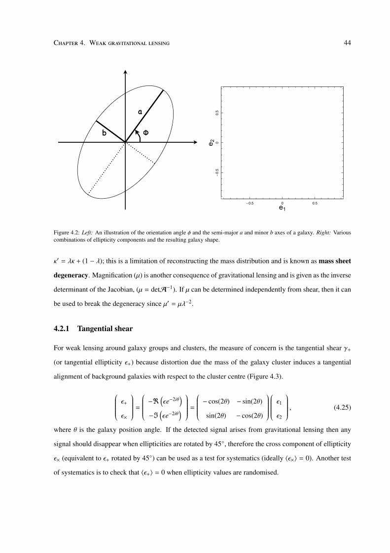
of these objects. We must rely on other observables as a proxy for mass.

Galaxy clusters are massive enough to gravitationally influence the light emitted from background

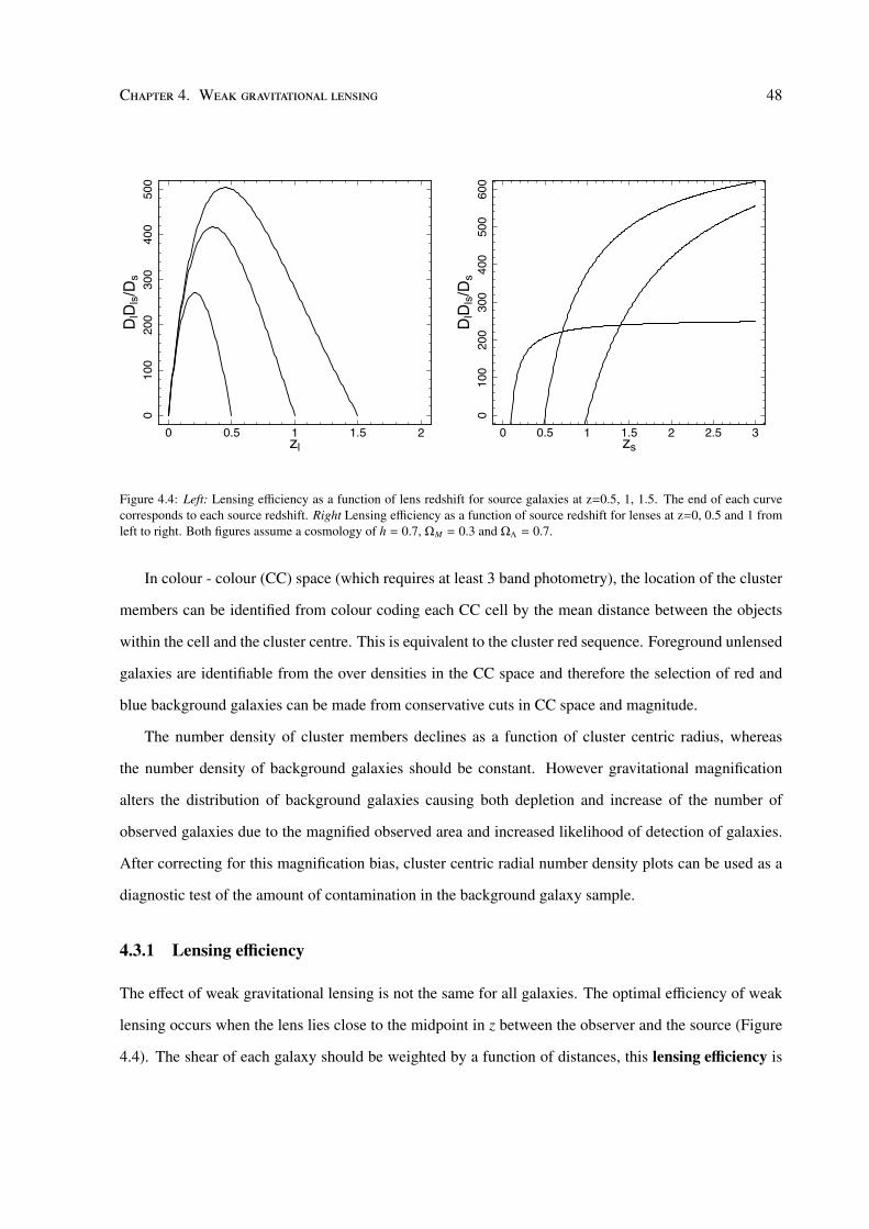
galaxies, an effect known as gravitational lensing. The mass of the galaxy cluster can be inferred from

the strength of the weak gravitational lensing signal. In principle this should be the best proxy for mass,

since it does not make many assumptions and is only dependent on the depth of the cluster gravita-

tional potential well. However as will be discussed in this thesis, weak gravitational lensing also has

its limitations arising from systematic uncertainties including shape measurement, photometric redshift

uncertainties and limited survey depth.

This thesis concerns constraining mass estimates of low mass groups and poor clusters, pushing the

mass limits that can achieved with ground-based weak lensing data.

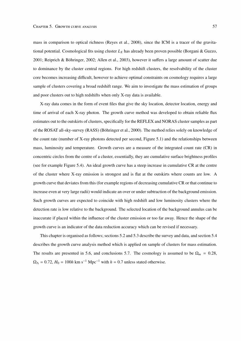
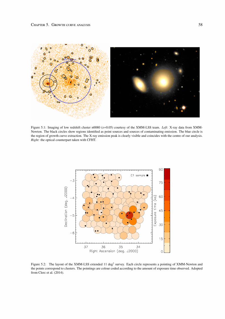
The first scientific chapter of this thesis uses X-ray data from pilot studies of the XXL survey to

obtain masses of a sample of 52 galaxy clusters. From the cumulative count rate profile and an exter-

nal luminosity – mass relation, the cluster luminosity and mass can be determined through an iterative

procedure. Although the estimated masses agree with those computed using an independent method, the

estimates are found to be highly dependent on the assumed external scaling relation, and may be sensitive

to the dynamical state of the cluster gas.

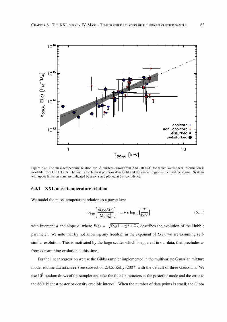
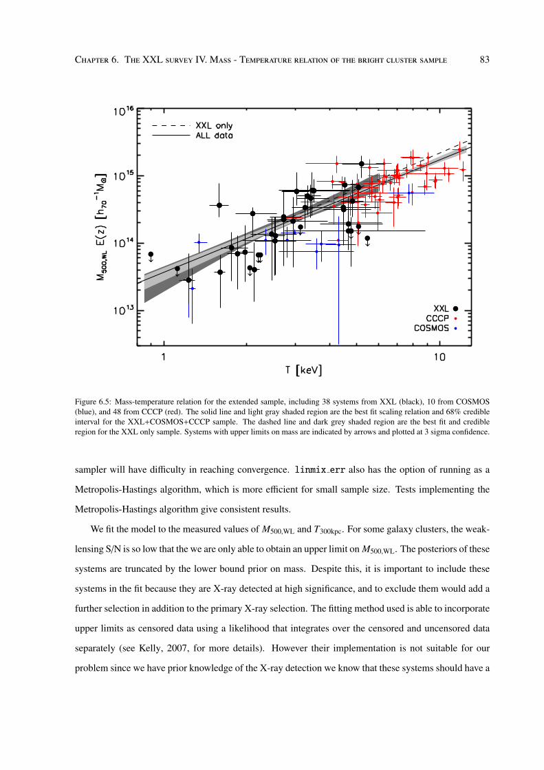
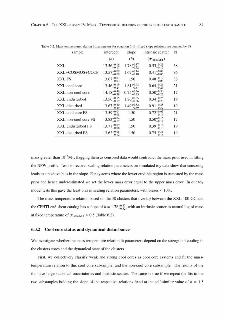
The second scientific chapter addresses this issue by taking a subsample of 38 XXL clusters to

calibrate a self-consistent weak lensing mass – X-ray temperature scaling relation. This is used to infer

the masses for the 100 clusters in the XXL bright sample appearing in several of the XXL first release

papers. The lensing masses are derived from the CFHTLenS weak lensing catalogue data where the

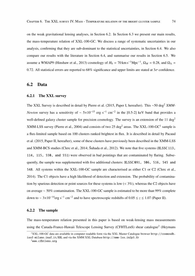
supreme quality of shape measurement, redshifts and survey depth allows us to obtain masses down

to ∼ 1013M without the need for stacking. The result when compared with hydrostatic mass based

relations suggest a mass dependent hydrostatic mass bias, potentially as high as 40% at the low mass

end. However as is shown later, it is only possible to obtain upper limits on the lowest signal-to-noise

systems and additional clusters from external samples are required to improve the constraints on the

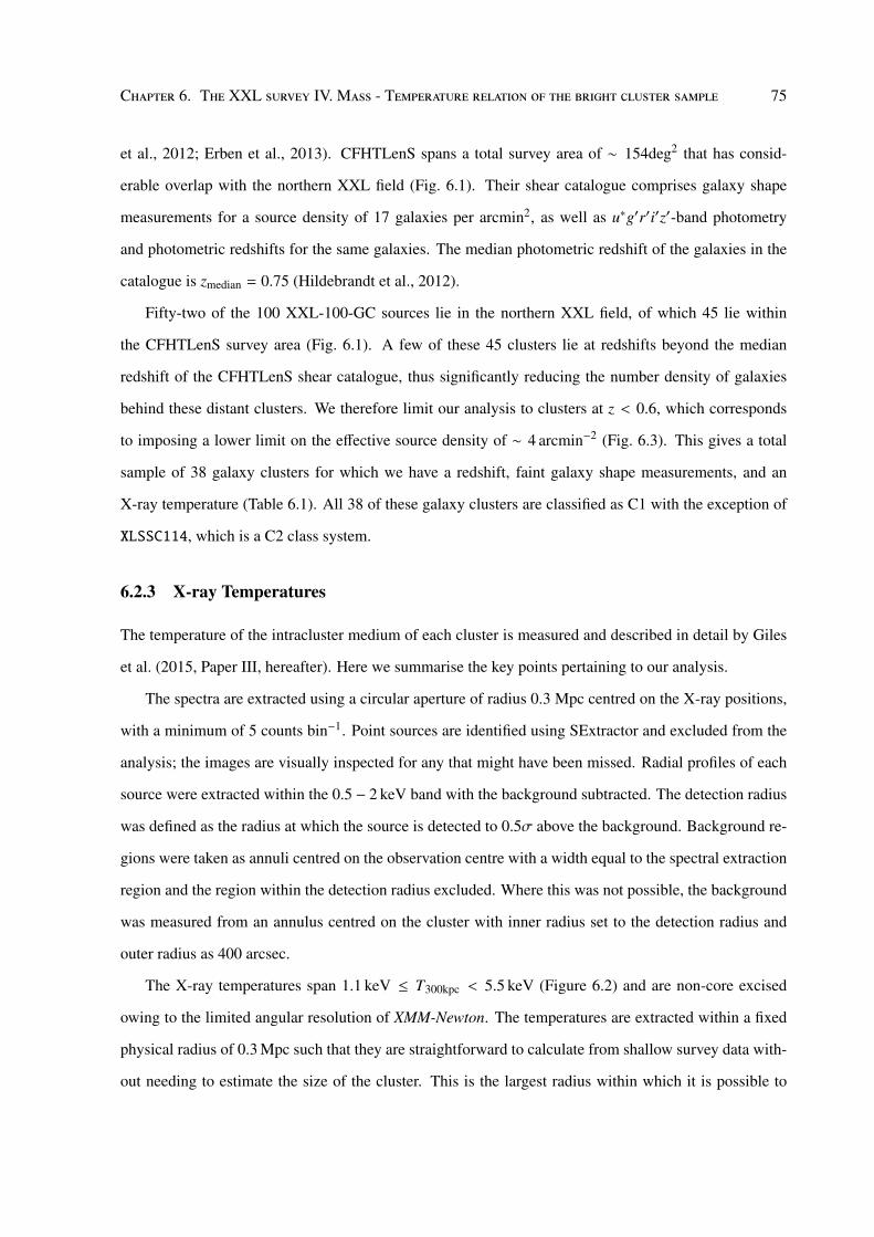
scaling relation parameters.

The final scientific chapter takes a new approach to cluster mass measurement by modelling the

problem top-down, inferring the individual cluster masses by modelling for the mass distribution of the

underlying population. This hierarchical model uses a quasi-stacking approach to simultaneously fit all

the data from the individual clusters. In this way we are able to constrain masses for objects with lower

signal-to-noise by using the population mean as a prior. I present a method to correctly use the results

from this work and derive from the data a mass-concentration relation. I also discuss how this method

could be extended to directly constrain cosmology, whilst eliminating some of the uncertainties that are

introduced through improper error propagation.

Dedication:

To my Grandma. Even though you aren’t here in person, I know you will always be with me in spirit. It

is through your love and support that made me who I am today. You are the bravest person I have ever

known and you inspire me even to this day.

Acknowledgements

I acknowledge a Postgraduate Studentship from the Science and Technology Facilities Council.

I would like to thank the University of Birmingham Astrophysics group for giving me an unforget-

table PhD experience. In particular David Stops for brightening up all my mornings without fail. I don’t

know how I would have survived these years without constantly harassing him for help. Equally, I thank

Hannah Middleton and Simon Stevenson for supporting me and my never-ending list of atrocious ideas.

I thank Sarah Mulroy for her support when all things go wrong and also Jim Barrett, Nicolas Clerc,

Michael Betancourt, Ian McCarthy, Alistair Sanderson and Trevor Sidery for useful discussions. I thank

the XXL collaboration for giving me the opportunity to lead groundbreaking research, especially Kate

Husband and Paul Giles who helped me survive the remote meetings and colossal treks!

I thank Prof Trevor Ponman and Dr Will Farr for providing prodigious supervision and advice on

even the most inane of topics. Lastly I would like to thank Dr Graham P. Smith for his endless support.

Statement of originality

The research presented in this thesis was undertaken at the Astrophysics & Space Research Group of

the University of Birmingham between October 2012 and March 2016. All work is my own except

where stated otherwise. The masses presented in chapter 5 are published in Clerc et al. (2014). Chapter

6 is a paper that has been accepted for publication (Lieu et al., 2015) and chapter 7 is a paper in prepara-

tion for submission. The work and writing of both papers are my own.

Maggie Lieu

30 March, 2016

Contents

1 Introduction 1

1.1 The expanding Universe . . . . . . . . . . . . . . . . . . . . . . . . . . . . . . . . . . 1

1.1.1 The Standard Model . . . . . . . . . . . . . . . . . . . . . . . . . . . . . . . . 3

1.1.2 Cosmological distances . . . . . . . . . . . . . . . . . . . . . . . . . . . . . . . 4

1.1.3 Growth of linear perturbations . . . . . . . . . . . . . . . . . . . . . . . . . . . 5

1.2 Groups and clusters of galaxies . . . . . . . . . . . . . . . . . . . . . . . . . . . . . . . 7

1.2.1 Cluster morphology . . . . . . . . . . . . . . . . . . . . . . . . . . . . . . . . 9

1.2.2 Multi-wavelength observations of galaxy clusters . . . . . . . . . . . . . . . . . 10

1.2.3 Clusters as cosmological probes . . . . . . . . . . . . . . . . . . . . . . . . . . 12

1.3 Summary, aims and structure of this thesis . . . . . . . . . . . . . . . . . . . . . . . . . 13

2 Mass proxies 15

2.1 Mass measurement . . . . . . . . . . . . . . . . . . . . . . . . . . . . . . . . . . . . . 15

2.1.1 Spherical overdensity mass . . . . . . . . . . . . . . . . . . . . . . . . . . . . . 15

2.1.2 Hydrostatic mass . . . . . . . . . . . . . . . . . . . . . . . . . . . . . . . . . . 16

2.1.3 Dynamical mass . . . . . . . . . . . . . . . . . . . . . . . . . . . . . . . . . . 17

2.1.4 Gravitational lensing mass . . . . . . . . . . . . . . . . . . . . . . . . . . . . . 17

2.2 The self similar model . . . . . . . . . . . . . . . . . . . . . . . . . . . . . . . . . . . 18

2.3 Scaling relations . . . . . . . . . . . . . . . . . . . . . . . . . . . . . . . . . . . . . . . 18

2.3.1 M–TX scaling relation . . . . . . . . . . . . . . . . . . . . . . . . . . . . . . . 19

2.3.2 LX–M scaling relation . . . . . . . . . . . . . . . . . . . . . . . . . . . . . . . 20

2.3.3 Other scaling relations . . . . . . . . . . . . . . . . . . . . . . . . . . . . . . . 21

2.3.4 Selection effects . . . . . . . . . . . . . . . . . . . . . . . . . . . . . . . . . . 22

2.4 Linear regression . . . . . . . . . . . . . . . . . . . . . . . . . . . . . . . . . . . . . . 23

2.4.1 BCES(Y|X) . . . . . . . . . . . . . . . . . . . . . . . . . . . . . . . . . . . . . 24

vi

Contents vii

2.4.2 Bisector . . . . . . . . . . . . . . . . . . . . . . . . . . . . . . . . . . . . . . . 25

2.4.3 Orthogonal . . . . . . . . . . . . . . . . . . . . . . . . . . . . . . . . . . . . . 25

2.4.4 MPFITEXY . . . . . . . . . . . . . . . . . . . . . . . . . . . . . . . . . . . . . . 25

2.4.5 linmix err . . . . . . . . . . . . . . . . . . . . . . . . . . . . . . . . . . . . 26

2.4.6 Error estimation . . . . . . . . . . . . . . . . . . . . . . . . . . . . . . . . . . 27

2.5 Summary . . . . . . . . . . . . . . . . . . . . . . . . . . . . . . . . . . . . . . . . . . 27

3 Bayesian inference 29

3.1 The Bayesics . . . . . . . . . . . . . . . . . . . . . . . . . . . . . . . . . . . . . . . . 29

3.1.1 Markov Chain Monte Carlo . . . . . . . . . . . . . . . . . . . . . . . . . . . . 30

3.2 The Metropolis Hastings algorithm . . . . . . . . . . . . . . . . . . . . . . . . . . . . . 30

3.2.1 Acceptance rate . . . . . . . . . . . . . . . . . . . . . . . . . . . . . . . . . . . 31

3.2.2 Proposal distribution . . . . . . . . . . . . . . . . . . . . . . . . . . . . . . . . 32

3.2.3 Priors . . . . . . . . . . . . . . . . . . . . . . . . . . . . . . . . . . . . . . . . 32

3.2.4 Convergence . . . . . . . . . . . . . . . . . . . . . . . . . . . . . . . . . . . . 33

3.2.5 Summary statistics . . . . . . . . . . . . . . . . . . . . . . . . . . . . . . . . . 35

3.3 Gibbs Sampling . . . . . . . . . . . . . . . . . . . . . . . . . . . . . . . . . . . . . . . 36

3.4 Hamiltonian Monte Carlo . . . . . . . . . . . . . . . . . . . . . . . . . . . . . . . . . . 36

3.5 Summary . . . . . . . . . . . . . . . . . . . . . . . . . . . . . . . . . . . . . . . . . . 39

4 Weak gravitational lensing 40

4.1 The lens equation . . . . . . . . . . . . . . . . . . . . . . . . . . . . . . . . . . . . . . 40

4.2 Shear and ellipticity . . . . . . . . . . . . . . . . . . . . . . . . . . . . . . . . . . . . . 42

4.2.1 Tangential shear . . . . . . . . . . . . . . . . . . . . . . . . . . . . . . . . . . 44

4.2.2 Shape measurement . . . . . . . . . . . . . . . . . . . . . . . . . . . . . . . . 45

4.3 Background galaxy selection . . . . . . . . . . . . . . . . . . . . . . . . . . . . . . . . 46

4.3.1 Lensing efficiency . . . . . . . . . . . . . . . . . . . . . . . . . . . . . . . . . 48

4.4 Dark matter halo density profiles . . . . . . . . . . . . . . . . . . . . . . . . . . . . . . 49

4.4.1 NFW profile . . . . . . . . . . . . . . . . . . . . . . . . . . . . . . . . . . . . 49

4.4.2 Centering . . . . . . . . . . . . . . . . . . . . . . . . . . . . . . . . . . . . . . 51

4.4.3 Triaxiality . . . . . . . . . . . . . . . . . . . . . . . . . . . . . . . . . . . . . . 51

Contents viii

4.5 The 2-halo term . . . . . . . . . . . . . . . . . . . . . . . . . . . . . . . . . . . . . . . 52

4.5.1 Large scale structure covariance . . . . . . . . . . . . . . . . . . . . . . . . . . 53

4.6 Alternative methods . . . . . . . . . . . . . . . . . . . . . . . . . . . . . . . . . . . . . 53

4.7 Summary . . . . . . . . . . . . . . . . . . . . . . . . . . . . . . . . . . . . . . . . . . 54

5 Growth curve analysis 56

5.1 Introduction . . . . . . . . . . . . . . . . . . . . . . . . . . . . . . . . . . . . . . . . . 56

5.2 Data . . . . . . . . . . . . . . . . . . . . . . . . . . . . . . . . . . . . . . . . . . . . . 59

5.3 Background subtraction . . . . . . . . . . . . . . . . . . . . . . . . . . . . . . . . . . . 59

5.4 The growth curve method . . . . . . . . . . . . . . . . . . . . . . . . . . . . . . . . . . 60

5.5 Selecting a luminosity–mass relation . . . . . . . . . . . . . . . . . . . . . . . . . . . . 61

5.6 Results . . . . . . . . . . . . . . . . . . . . . . . . . . . . . . . . . . . . . . . . . . . . 67

5.6.1 Quality flag . . . . . . . . . . . . . . . . . . . . . . . . . . . . . . . . . . . . . 67

5.6.2 Comparison with the literature . . . . . . . . . . . . . . . . . . . . . . . . . . . 68

5.7 Summary . . . . . . . . . . . . . . . . . . . . . . . . . . . . . . . . . . . . . . . . . . 69

6 The XXL survey IV. Mass - Temperature relation of the bright cluster sample 71

6.1 Introduction . . . . . . . . . . . . . . . . . . . . . . . . . . . . . . . . . . . . . . . . . 72

6.2 Data . . . . . . . . . . . . . . . . . . . . . . . . . . . . . . . . . . . . . . . . . . . . . 74

6.2.1 The XXL survey . . . . . . . . . . . . . . . . . . . . . . . . . . . . . . . . . . 74

6.2.2 The sample . . . . . . . . . . . . . . . . . . . . . . . . . . . . . . . . . . . . . 74

6.2.3 X-ray Temperatures . . . . . . . . . . . . . . . . . . . . . . . . . . . . . . . . 75

6.2.4 Cool core strength . . . . . . . . . . . . . . . . . . . . . . . . . . . . . . . . . 76

6.2.5 Weak gravitational lensing . . . . . . . . . . . . . . . . . . . . . . . . . . . . . 77

6.3 Results . . . . . . . . . . . . . . . . . . . . . . . . . . . . . . . . . . . . . . . . . . . . 81

6.3.1 XXL mass-temperature relation . . . . . . . . . . . . . . . . . . . . . . . . . . 82

6.3.2 Cool core status and dynamical disturbance . . . . . . . . . . . . . . . . . . . . 84

6.3.3 Combination with other samples . . . . . . . . . . . . . . . . . . . . . . . . . . 85

6.3.4 Mass estimates for XXL-100-GC . . . . . . . . . . . . . . . . . . . . . . . . . 87

6.4 Discussion . . . . . . . . . . . . . . . . . . . . . . . . . . . . . . . . . . . . . . . . . . 87

6.4.1 Systematic uncertainties . . . . . . . . . . . . . . . . . . . . . . . . . . . . . . 88

Contents ix

6.4.2 Comparison with the literature . . . . . . . . . . . . . . . . . . . . . . . . . . . 92

6.5 Summary . . . . . . . . . . . . . . . . . . . . . . . . . . . . . . . . . . . . . . . . . . 94

7 Hierarchical modelling 101

7.1 Introduction . . . . . . . . . . . . . . . . . . . . . . . . . . . . . . . . . . . . . . . . . 101

7.2 Method . . . . . . . . . . . . . . . . . . . . . . . . . . . . . . . . . . . . . . . . . . . 104

7.2.1 Hyperparameters . . . . . . . . . . . . . . . . . . . . . . . . . . . . . . . . . . 105

7.2.2 Sample parameters . . . . . . . . . . . . . . . . . . . . . . . . . . . . . . . . . 106

7.2.3 Model fitting . . . . . . . . . . . . . . . . . . . . . . . . . . . . . . . . . . . . 107

7.3 Data . . . . . . . . . . . . . . . . . . . . . . . . . . . . . . . . . . . . . . . . . . . . . 108

7.4 Bayesian model . . . . . . . . . . . . . . . . . . . . . . . . . . . . . . . . . . . . . . . 108

7.4.1 Scaling relations . . . . . . . . . . . . . . . . . . . . . . . . . . . . . . . . . . 111

7.5 Results . . . . . . . . . . . . . . . . . . . . . . . . . . . . . . . . . . . . . . . . . . . . 111

7.5.1 Global estimates . . . . . . . . . . . . . . . . . . . . . . . . . . . . . . . . . . 111

7.5.2 Mass estimates . . . . . . . . . . . . . . . . . . . . . . . . . . . . . . . . . . . 113

7.5.3 Shrinkage . . . . . . . . . . . . . . . . . . . . . . . . . . . . . . . . . . . . . . 115

7.5.4 Mass – concentration relation . . . . . . . . . . . . . . . . . . . . . . . . . . . 115

7.5.5 Tests on priors . . . . . . . . . . . . . . . . . . . . . . . . . . . . . . . . . . . 117

7.5.6 Discussion . . . . . . . . . . . . . . . . . . . . . . . . . . . . . . . . . . . . . 118

7.6 Summary . . . . . . . . . . . . . . . . . . . . . . . . . . . . . . . . . . . . . . . . . . 120

8 Conclusion 124

References 127

List of Figures

1.1 Linear and non linear matter power spectrum at z=1 and assuming a WMAP9 cosmology

(Hinshaw et al., 2013), from the halofit program (Smith et al., 2003). . . . . . . . . . 5

1.2 Mass variance (left) and mass function (right) at z=1 (solid line) and z=2 (dashed line)

assuming Tinker et al. (2008) fitting function and WMAP9 cosmological parameters.

This is plotted using the HMFcalc tool from Murray et al. (2013a). . . . . . . . . . . . . 6

2.1 Left: The effect of Malmquist bias on the LX–M scaling relation of a flux limited sample

of clusters. The red and black points show the clusters within the population and the red

solid line shows the line of best fit. After applying a cut in flux (dashed line), the fit to the

selected sample of clusters (solid black line) is shallower than the underlying population

relation. Right: The effect of Eddington bias on the LX–M scaling relation. The black

line is the fit to the unscattered variables (black points), and the red line is the fit to the

scattered variables (red points). . . . . . . . . . . . . . . . . . . . . . . . . . . . . . . . 22

3.1 Left: The Uniform and Jeffreys prior probability distributions. Right: Again the Uni-

form and Jeffreys priors distributions but the y axis is plotted as P(ln x) assuming scale

invariance∫

P(x) dx =∫

P(ln x) d ln x. It shows that the Jeffreys prior is uniform on log

interval scales. . . . . . . . . . . . . . . . . . . . . . . . . . . . . . . . . . . . . . . . 32

3.2 Traceplots of an MCMC sample, left is an example of a chain that has good mixing. Mid-

dle shows moderate mixing, the samples fluctuate about the convergence value, however

the steps are small so will require a lot of thinning to remove the correlation between

samples. Right is an example of bad mixing, the samples do not converge. . . . . . . . . 34

3.3 Left: Posterior sampling of a target distribution (red) with metropolis-hastings algorithm

assuming a gaussian proposal distribution. Right: Sampling of the posterior with Gibbs

sampling, note that each sample xi is taken after the all parameters have been sampled. . 36

4.1 A schematic diagram of a typical gravitational lens system. . . . . . . . . . . . . . . . 41

x

List of Figures xi

4.2 Left: An illustration of the orientation angle φ and the semi-major a and minor b axes of

a galaxy. Right: Various combinations of ellipticity components and the resulting galaxy

shape. . . . . . . . . . . . . . . . . . . . . . . . . . . . . . . . . . . . . . . . . . . . . 44

4.3 An illustration of the tangential and cross ellipticity of galaxy sources at different loca-

tions with respect to a centre point. The components of the ellipticity are assumed to be

ε1 = 0.7 and ε2 = 0 for all 3 galaxies however the tangential and cross components of

the ellipticity are dependent on the position angle θ. . . . . . . . . . . . . . . . . . . . 45

4.4 Left: Lensing efficiency as a function of lens redshift for source galaxies at z=0.5, 1, 1.5.

The end of each curve corresponds to each source redshift. Right Lensing efficiency as

a function of source redshift for lenses at z=0, 0.5 and 1 from left to right. Both figures

assume a cosmology of h = 0.7, ΩM = 0.3 and ΩΛ = 0.7. . . . . . . . . . . . . . . . . 48

5.1 Imaging of low redshift cluster n0080 (z=0.05) courtesy of the XMM-LSS team. Left: X-

ray data from XMM-Newton. The black circles show regions identified as point sources

and sources of contaminating emission. The blue circle is the region of growth curve

extraction. The X-ray emission peak is clearly visible and coincides with the centre of

our analysis. Right: the optical counterpart taken with CFHT. . . . . . . . . . . . . . . 58

5.2 The layout of the XMM-LSS extended 11 deg2 survey. Each circle represents a pointing

of XMM-Newton and the points correspond to clusters. The pointings are colour coded

according to the amount of exposure time observed. Adopted from Clerc et al. (2014). . 58

5.3 A comparison of the growth curve mass estimates assuming various luminosity mass

scaling relations from Sun (2012); Pratt et al. (2009); Reichert et al. (2011) and Leau-

thaud et al. (2010), given equality (dashed line) and non error weighted mass bias cal-

culated as B = exp(〈ln(Mx/My)〉) where Mx and My are the M500 values for the corre-

sponding x and y axes respectively. . . . . . . . . . . . . . . . . . . . . . . . . . . . . 62

List of Figures xii

5.4 Growth curves of the galaxy clusters in this study assuming the Sun, self similar luminosity–

mass relation to fit the r500 value (solid black vertical line). On the y axis is the cumu-

lative count rate or interchangeably X-ray flux or luminosity. The scale is not plotted

due the large range of cumulative count rates between the clusters (with peaks as low

as 0.01ct/s and as high as 1ct/s) but starts at 0 counts s−1. The x axis is given as radial

distance from the X-ray peak position in arcseconds. The shaded gray is the 1σ error on

the cumulative count rate and the diagonal shading represents the background annulus

region. . . . . . . . . . . . . . . . . . . . . . . . . . . . . . . . . . . . . . . . . . . . 65

5.5 Left: Growth curve masses in the mass temperature plane. The size of the points corre-

sponds to the quality grade, with A grade objects being the largest and C grade objects

being the smallest. Clusters are colour coded with respect to their redshifts and compared

to mass–temperature relations from Arnaud et al. (2005); Sun et al. (2009) and Vikhlinin

et al. (2009). Right: Growth curve luminosities as a function of redshift and coloured

with respect to the X-ray temperature values. The dashed line represents the soft band

([0.5-2] keV) flux limit of FX = 4 × 10−15 erg s−1 cm−2. . . . . . . . . . . . . . . . . . 68

5.6 Comparison of measured variables, M500 (left) and bolometric L500 (right) using beta

model fitting (Clerc et al., 2014) and growth curve methods where the dotted line repre-

sents equality. . . . . . . . . . . . . . . . . . . . . . . . . . . . . . . . . . . . . . . . 69

6.1 Overlap of XXL-100-GC with the CFHTLenS W1 field. The boxes are individual point-

ings in CFTHT with XXL-North field clusters (filled points). The shaded boxes are

pointings that fail the CFHTLenS weak-lensing field selection criteria (See §6.4.1). . . . 73

6.2 Redshift versus X-ray temperature T300kpc for the 38 clusters from XXL-100-GC that are

located within the CFHTLenS shear catalogue footprint. . . . . . . . . . . . . . . . . . 76

6.3 Left: Number density of background galaxies behind each galaxy cluster versus cluster

redshift. Right: Weak-lensing shear signal-to-noise ratio as a function of cluster redshift. 77

6.4 The mass-temperature relation for 38 clusters drawn from XXL-100-GC for which weak-

shear information is available from CFHTLenS. The line is the highest posterior density

fit and the shaded region is the credible region. Systems with upper limits on mass are

indicated by arrows and plotted at 3 σ confidence. . . . . . . . . . . . . . . . . . . . . 82

List of Figures xiii

6.5 Mass-temperature relation for the extended sample, including 38 systems from XXL

(black), 10 from COSMOS (blue), and 48 from CCCP (red). The solid line and light

gray shaded region are the best fit scaling relation and 68% credible interval for the

XXL+COSMOS+CCCP sample. The dashed line and dark grey shaded region are the

best fit and credible region for the XXL only sample. Systems with upper limits on mass

are indicated by arrows and plotted at 3 sigma confidence. . . . . . . . . . . . . . . . . 83

6.6 Surface brightness concentration (CSB) parameter versus the offset between X-ray cen-

troid and BCG as a fraction of weak-lensing r500,WL. The horizontal dashed line at CSB

= 0.075 indicates the separation of cool core and non-cool core classed systems. The

vertical dashed line at δr/r500,WL = 0.05 separates undisturbed and disturbed clusters.

The grey shaded region shows the overlap between cool core and undisturbed clusters.

There is no observed correlation between the CSB parameter and the centering offset

despite the theory that both are indicators of cluster dynamical state. . . . . . . . . . . . 86

6.7 Comparison of core excised X-ray temperatures (Kettula et al., 2013) and the re-derived

temperatures measured within a 0.3Mpc aperture. The dashed line is equality. . . . . . . 87

6.8 Left: Comparison of our results on the slope of the mass-temperature relation with those

in the literature (Eckmiller et al., 2011; Lovisari et al., 2015; Sun et al., 2009; Vikhlinin

et al., 2009). Right: Comparison of the mass of a cluster of temperature T = 3 keV at

z = 0.3 based on mass-temperature relations and those in the literature. In both panels,

filled circles are samples that use weak-lensing masses, open diamonds are samples that

use hydrostatic masses. The COSMOS+CCCP+160D and COSMOS-only relations are

from Kettula et al. (2013) and the CFHTLS relation from Kettula et al. (2015). The other

two Kettula et al. (2015) relations include COSMOS and CCCP clusters and BC has been

corrected for Eddington bias. . . . . . . . . . . . . . . . . . . . . . . . . . . . . . . . 88

6.9 Tangential and cross-component ellipticity as a function of distance from cluster centre. 96

6.10 Tangential and cross-component ellipticity as a function of distance from cluster centre.

Here upper limit mass estimates are measured for XLSSC57 and XLSSC85. . . . . . . . . 97


Here upper limit mass estimates are measured for XLSSC90, XLSSC92 and XLSSC96. . . 98

List of Figures xiv


Here upper limit mass estimates are measured for XLSSC99 and XLSSC108. . . . . . . . 99

6.13 Tangential and cross component ellipticity as a function of distance from cluster centre.

Here upper limit mass estimates are measured for XLSSC115. . . . . . . . . . . . . . . 100

7.1 Posterior distributions of the 9 hyperparameters, where the subscripts 1,2,3 represent

ln(M200), ln(c200) and ln(1 + z) respectively. The red contours show 68, 95 and 99% con-

fidence intervals, the histograms show the marginalised parameters with dashed vertical

lines at 2σ. Left: Global mean vector parameters Right: Covariance matrix elements. . 109

7.2 Left& center: Comparison of the posteriors for the population mean (solid blue) and the

posteriors for the individual clusters (solid grey) for mass and concentration respectively.

A gaussian distribution centred on the population mean and with a standard deviation

from the covariance matrix is also shown (dashed blue). Right: The z distribution of

the population plotted as a gaussian centred on a mean and standard deviation obtained

from the global mean vector and covariance matrix (dashed blue). It agrees well with the

spectroscopic redshift distribution of the sample (solid grey). From this we can conclude

that the data is able to constrain the individual cluster masses reasonably well, as the

individual mass posteriors appear independent of the population mass posterior. On the

contrary, the individual concentrations are completely dominated by the posterior of the

population concentration, which implies that without the hierarchical model, individual

cluster concentrations would not be possible. . . . . . . . . . . . . . . . . . . . . . . . 112

7.3 Comparison between the masses measured with the hierarchical method and those mea-

sured in chapter 6. The dashed lined shows equality. The black circles are masses where

they assume a fixed c–M relation from Duffy et al. (2008) and the blue triangles are where

they allow concentration to be free. Our mass estimates show a systematic difference that

is expected from the nature of the hierarchical model in that for high mass clusters we

predict lower masses and low mass groups we predict higher mass values. The influence

of the population distribution is more pronounced for the low mass systems where the

uncertainties on the data are larger. . . . . . . . . . . . . . . . . . . . . . . . . . . . . 113

List of Figures xv

7.4 Individual galaxy cluster mass shrinkage estimates show the individual mass estimates

shrink towards the population mean as σ2ln M decreases. Each cluster is represented as

a different colour. The points show the fitted individual masses of clusters using the

hierarchical method where σ2ln M is 1.79 and the shaded region is the 1σ error. The stars

and crosses are the individual masses following a non-hierarchical method chapter 6

where concentration is a free parameter and where concentration is fixed to the Duffy

et al. (2008) c–M relation respectively. . . . . . . . . . . . . . . . . . . . . . . . . . . 114

7.5 Concentration – mass relation. c values are computed for all M values in the range using

the equation 7.18 for each pair of µ and Σ sampled. The mean and 1σ uncertainty is

shown as the solid black and dotted lines respectively. The fitted covariance and mean of

population concentration and mass shown by red contours of 1, 2 and 3σ confidence and

therefore appear mis-aligned from the fit. For comparison, the solid purple line shows

the Duffy et al. (2008) c–M relation at our population mean redshift z=0.27 and the solid

green line is the Dutton & Maccio (2014) relation for NFW haloes at z=0.5. The black

points are the mean of the individual log parameters. . . . . . . . . . . . . . . . . . . . 116

7.6 Posteriors of the regression parameters, the dotted line represents the mean. It is clear that

although the normalisation prefers lower values, the uncertainty is large and we cannot

completely rule out higher normalisations. Similarly the uncertainty on the evolution

parameter γ but is fully consistant with no evolution whereas the slope β much better

constrained. . . . . . . . . . . . . . . . . . . . . . . . . . . . . . . . . . . . . . . . . . 117

7.7 Posterior of concentration width Σ22 (solid black), and the prior function Pr(τ|µτ =

0, στ = 2.5) (dashed blue). The large scale parameter used in the prior allows even

very high values of σ2ln(c) and the results is not dominated by the prior on τ. . . . . . . . 118

7.8 The posterior distribution functions of the individual mass measurements (solid black

line) and the fit statistic taken as the posterior mean (dotted black line). The grey shaded

regions show the posteriors of the individual masses from chapter 6 assuming a free

concentration parameter for comparison. The truncation at the lower prior bound of

1013 M is a visible feature of the upper limit systems (subsection 6.3.1). . . . . . . . . 122

List of Figures xvi

7.9 Test of prior sensitivity on the global mean vector. X-axis is the centre of the gaussian

prior on mass and the y-axis is the centering of the gaussian prior on concentration.

Each individual plot shows the confidence ellipse based on the mean covariance matrix

centred on the mean global mean vector at 1,2 and 3σ. Black dot represents the prior

center, vertical and horizontal lines show the population mean mass and concentration

respectively, with 1σ uncertainty shaded grey. . . . . . . . . . . . . . . . . . . . . . . 123

List of Tables

5.1 Compilation of mass-luminosity scaling relations from the literature (Pratt et al., 2009;

Reichert et al., 2011; Sun, 2012; Leauthaud et al., 2010) used in mass estimation where

NE, SS, CC, NC correspond to no-evolution, self similar evolution, cool core corrected

and non cool core corrected respectively. The scaling relations are in the form of M =

A(LxE(z)C)B in units 10−10Mh−170 . Column 5 is the fitting method (see section 2.4) and

column 6 is whether point sources are excised (y) or (n). Column 7 is the temperature

range in units keV, 8 is X-ray luminosity range in units 1044erg s−1, 9 is luminosity band

in keV or bolometric and 10 is the redshift range. . . . . . . . . . . . . . . . . . . . . . 61

5.2 Estimated growth curve masses for clusters using Sun et al. (2009) self similar M-L

relation - Quality flag (column 2) where A is good, B is satisfactory, C is unsatisfactory

in terms of reliability for mass estimation. Provided is r500 (column 3), L500 (column 4),

M500 (column 5) and bolometric conversion factor (column 6) values. . . . . . . . . . . 66

6.1 Cluster properties and mass estimates. . . . . . . . . . . . . . . . . . . . . . . . . . . . 80

6.2 Mass-temperature relation fit parameters for equation 6.11. Fixed slope relations are

denoted by FS. . . . . . . . . . . . . . . . . . . . . . . . . . . . . . . . . . . . . . . . 84

xvii

Chapter 1

Introduction

The motivation of this research is to facilitate the effort of using galaxy groups and clusters to constrain

cosmological parameters. Specifically, pushing the boundaries of mass measurement down to ∼ 1013 M,

where the majority of X-ray groups are detected. Here I provide introduction to cosmology, where the

many of the equations can be found in any cosmology text book (e.g. Ryden, 2003). I will also introduce

galaxy groups and clusters, so that by the end of this chapter, it should be clear what they are, why they

are such interesting systems and their role in cosmology (for further reading I would suggest Voit, 2005;

Borgani, 2008; Allen et al., 2011). This chapter provides the basic concepts required to understand the

goal of this thesis and the structure will be outlined at the end of this chapter.

1.1 The expanding Universe

One of the most important discoveries of cosmology occurred in 1929 by Edwin Hubble, who whilst

working on a relationship between the recession velocity of distant galaxies and their distance, found

that all distant galaxies are moving away from us. This implies that Universe is expanding. Extrapolating

back in time, leads to the Big Bang Theory, according to which the Universe originated at an infinitely

hot and dense state. In the Big Bang model, the Universe began as a photon-baryon plasma which

through adiabatic expansion, cooled enough for neutral hydrogen to form and consequently for photons to

decouple from matter leaving behind a relic radiation that was first observed by Penzias & Wilson (1965).

This almost uniform ∼ 2.73K thermal radiation, pervades the observable Universe and is known as the

cosmic microwave background (CMB). With this discovery a new problem was introduced; any two

areas on the sky separated by over ∼ 2 should not have had time to be in causal contact. This dilemma

can be solved by including a period of exponential expansion during the early Universe (inflation).

Observations of Type Ia supernovae (SNeIa) indicate that the Universe is still expanding today and at an

accelerated rate. Currently the leading explanation for cosmic expansion is an unknown form of energy,

1

Chapter 1. Introduction 2

dark energy, and it potentially exists in the form of the cosmological constant Λ, first introduced by

Einstein in his Theory of General Relativity (Einstein, 1915). In the standard model of cosmology or

ΛCDM, the total mass-energy of the Universe is comprised of ∼ 70% dark energy and ∼ 25% cold dark

matter (CDM).

The majority of matter is in the form of dark matter (DM), so it is not surprise that the cosmological

parameters are sensitive to its abundance and form.Observational evidence of dark matter trace back to

Oort (1932), who from the orbital velocities of stars in the milky way deduced that stars alone could only

account for about a third of the total mass. DM has yet to be directly observed, largely owing to the fact

that it does not emit electromagnetic radiation, however other indications of its existence is supported by

observations of merging galaxy clusters (a topic that will be returned to later in section 1.2.2).

Possible candidates of dark matter include massive compact halo objects (MACHOs), neutrinos, ax-

ions and weakly interacting particles (WIMPs) (Baltz, 2004). MACHOs are made of ordinary baryonic

matter and include neutron stars, black holes and brown dwarves. The elemental abundance predicted

from Big Bang nucleosynthesis implies that DM is non-baryonic, so MACHOs are unlikely to com-

pletely account for dark matter. Neutrinos are highly relativistic particles and are therefore a hot dark

matter (HDM). Observational studies indicate that the Universe formed hierarchically, with galaxies

forming first and eventually merging to form the larger structures of groups and clusters (Kravtsov &

Borgani, 2012). This theory of structure formation is in better agreement with CDM simulations as op-

posed those of HDM which predicts the largest structures form first due to the larger streaming lengths.

Axions are a hypothetical, non-relativistic particle of low mass and neutral charge. In order for axions to

explain dark matter, they must have a very specific mass and should decay into a pair of photons. WIMPs

are the most favoured DM candidate since they are also predicted from extensions of the Standard Model

of particle physics. These particles only interact via the weak force and gravity, and if they exist their

predicted abundance would coincide with the amount of dark matter we observe in the Universe. Ex-

periments including the Axion Dark matter experiment1, LUX2, SuperCDMS3 and even the LHC4 have

been looking for evidence of a dark matter particle but so far without prevail.

1http://depts.washington.edu/admx/index.shtml2http://luxdarkmatter.org3http://cdms.berkeley.edu4http://home.cern/topics/large-hadron-collider

http://depts.washington.edu/admx/index.shtml

http://luxdarkmatter.org

http://cdms.berkeley.edu

http://home.cern/topics/large-hadron-collider


1.1.1 The Standard Model

On large scales, the Universe obeys the cosmological principle; it is both isotropic and homogeneous. It

can be described by the Friedmann-Lemaıtre-Robertson-Walker (FLRW) metric.

ds2 = −c2dt2 + a(t)2[dr2 + S κ(r)2(dθ2 + sin2 θdφ2)

]. (1.1)

Here c2dt2 accounts for the time component and the latter half of the equation is the spatial component

where S κ(r) is governed by the three possible types of curvature of the Universe. The scale factor, a = a(t)

characterises the amount of expansion of the Universe at time t; for convenience, this is normalised to

the present day value of a0 = a(t0) = 1. The wavelength of light emitted by a distant astronomical object

is shifted as the Universe expands and this is characterised by the redshift z which is related to the scale

factor in the following way,

z =λo − λe

λe=

a(t0)a(te)

− 1 =1

a(te)− 1 (1.2)

where λe, te are the wavelength and time at which the light from the object is emitted and λo, t0 are the

wavelength and time at which it is observed.

The Hubble parameter describes the rate of expansion of the Universe

H(z) =aa

(1.3)

where a is the time derivative of a. It is known as the Hubble constant when evaluated at the present day

and is commonly expressed in terms of a dimensionless hubble parameter h, H0 = aa |t=t0 = 100 h km s−1 Mpc−1

where h ' 0.7.

Einstein’s field equations are a set of 10 equations that describe gravity. The Friedmann equations

are a solution to Einstein’s field equations for the FLRW metric. The two equations describe the rate of

expansion of an isotropic and homogenous Universe in terms of the mass density ρ and pressure p. The

first of which is

H(z)2 =

( aa

)2=

8πG3ρ −

κc2

a2 (1.4)

where G is the gravitational constant, κ is the curvature and c is the speed of light in a vacuum. For a

spatially flat (κ = 0) Universe, the current density is the critical density

ρcrit,0 =3H2

0

8πG= 2.77 × 1011h2 MMpc−3. (1.5)


At a redshift z, the critical density is ρcrit(z) =3H(z)2

8πG . In the simplest case ΛCDM Universe, the Fried-

mann equations can be rewritten in terms of the density parameters

H(z)H0

=√

ΩR(1 + z)−4 + ΩM(1 + z)−3 + Ωκ(1 + z)−2 + ΩΛ, (1.6)

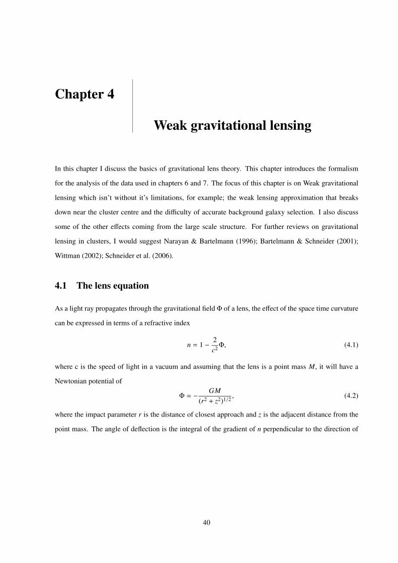
where ΩR, ΩM, Ωκ and ΩΛ are the present-day radiation, matter, curvature and dark energy densities

with respect to the critical density. In a flat Universe the curvature term is negligible, and the radiation

term becomes negligible at late epochs. The evolution scaling parameter can therefore be expressed as

E(z) =H(z)H0

=√

ΩM(1 + z)−3 + ΩΛ. (1.7)

1.1.2 Cosmological distances

The distance to a cosmological object is ambiguous due to the curvature and expanding nature of our

Universe. The comoving distance is perhaps the most straight forward measure of distance,

Dc(t0) = c∫ t0

te

dta(t)

. (1.8)

It is defined as the distance measured along the spatial geodesic between 2 points that accounts for the

expansion. However, the comoving distance to an object is not directly measurable. For astronomers, a

property that is observable is the amount of flux emitted by an object. Flux is usually measured within a

limited wavelength range, but when integrated over all wavelengths it is known as the bolometric flux.

For standard candles, an object of known luminosity, a convenient distance measure is the luminosity distance

DL, defined by its bolometric flux (F) and luminosity (L)

DL =

( L4πF

) 12. (1.9)

When the object of interest is not a standard candle, but is instead a standard ruler of a known actual size

l, and apparent angular size δθ, the angular diameter distance is used

DA =lδθ. (1.10)

These 3 distance measures are related to each other in the following way

DL = Dc(t0) (1 + z) = DA (1 + z)2. (1.11)


10−3 10−2 10−1 100 101

0.01

0.1

110

100

1000

P(k)[Mpc

3 h−3]

k[Mpc/h]

linearnon-linear

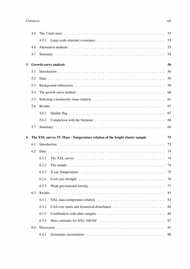
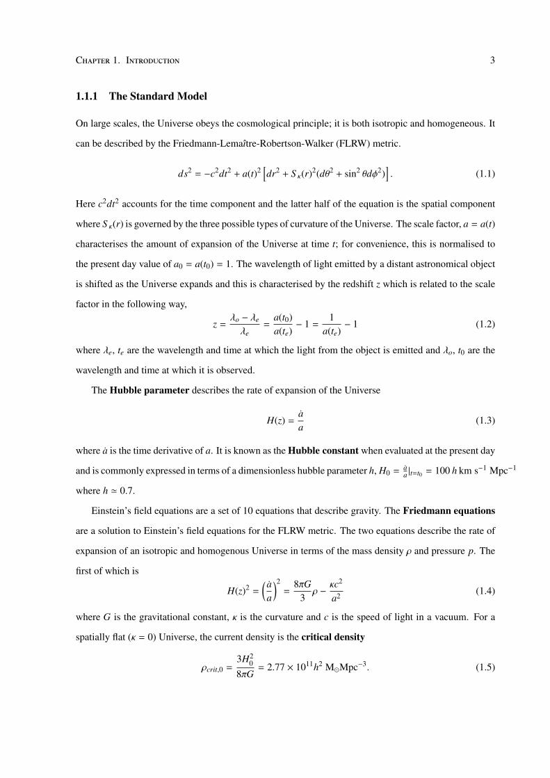
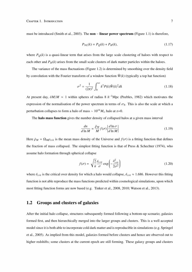
Figure 1.1: Linear and non linear matter power spectrum at z=1 and assuming a WMAP9 cosmology (Hinshaw et al., 2013),from the halofit program (Smith et al., 2003).

1.1.3 Growth of linear perturbations

The nodes, filaments and voids of the large scale structure observed today, originate from initial quantum

fluctuations in the early Universe that have been enhanced by cosmic expansion and self-gravity. These

density perturbations have been verified by temperature perturbations observed in the CMB; they are

characterised by the density contrast

δ(x) =ρ(x) − ρ

ρ(1.12)

where ρ(x) is the density at coordinate x and ρ is mean density. In a homogeneous Universe, δ ' 0 and

so higher order statistics are required in order to describe them.

The two point correlation function describes the probability of variation from uniformity, which in

Fourier space, is the power spectrum (Figure 1.1). For density contrast, the linear matter power spectrum

is

P(k) = 〈| ˆδ(k)|2〉, (1.13)

where ˆδ(k) denotes the Fourier transform of δ as a function of wavenumber (or wavelength λ) k = 2π/λ.

The fluctuations can be treated as a gaussian field, where the power spectrum contains all the statistical


1010 1011 1012 1013 1014 1015

0.5

12

M [Msol/h]

σ

1010 1011 1012 1013 1014 1015

10−7

10−6

10−5

10−4

10−3

10−2

M [Msol/h]dn

/dln

M [h

3 Mpc

−3]

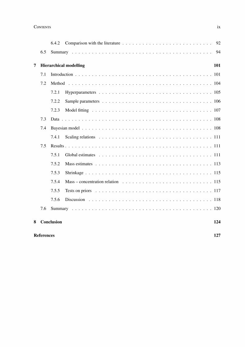
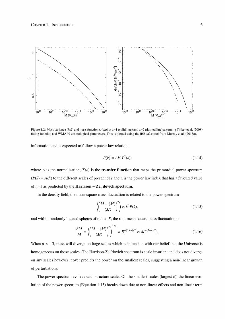
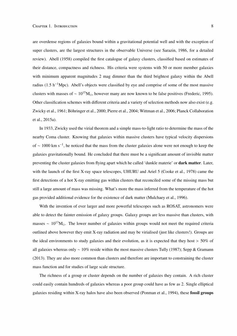
Figure 1.2: Mass variance (left) and mass function (right) at z=1 (solid line) and z=2 (dashed line) assuming Tinker et al. (2008)fitting function and WMAP9 cosmological parameters. This is plotted using the HMFcalc tool from Murray et al. (2013a).

information and is expected to follow a power law relation:

P(k) = AknT 2(k) (1.14)

where A is the normalisation, T (k) is the transfer function that maps the primordial power spectrum

(P(k) = Akn) to the different scales of present day and n is the power law index that has a favoured value

of n=1 as predicted by the Harrison − Zel′dovich spectrum.

In the density field, the mean square mass fluctuation is related to the power spectrum⟨(M − 〈M〉〈M〉

)2⟩∝ k3P(k), (1.15)

and within randomly located spheres of radius R, the root mean square mass fluctuation is

δMM

=

⟨(M − 〈M〉〈M〉

)2⟩1/2

∝ R−(3+n)/2 ∝ M−(3+n)/6. (1.16)

When n < −3, mass will diverge on large scales which is in tension with our belief that the Universe is

homogeneous on those scales. The Harrison-Zel’dovich spectrum is scale invariant and does not diverge

on any scales however it over predicts the power on the smallest scales, suggesting a non-linear growth

of perturbations.

The power spectrum evolves with structure scale. On the smallest scales (largest k), the linear evo-

lution of the power spectrum (Equation 1.13) breaks down due to non-linear effects and non-linear term


must be introduced (Smith et al., 2003). The non − linear power spectrum (Figure 1.1) is therefore,

PNL(k) = PQ(k) + PH(k), (1.17)

where PQ(k) is a quasi-linear term that arises from the large scale clustering of haloes with respect to

each other and PH(k) arises from the small scale clusters of dark matter particles within the haloes.

The variance of the mass fluctuations (Figure 1.2) is determined by smoothing over the density field

by convolution with the Fourier transform of a window function W(k) (typically a top hat function)

σ2 =1

(2π)2

∫ ∞

0k2P(k)W(k)2dk (1.18)

At present day, δM/M ' 1 within spheres of radius 8 h−1Mpc (Peebles, 1982) which motivates the

expression of the normalisation of the power spectrum in terms of σ8. This is also the scale at which a

perturbation collapses to form a halo of mass ∼ 1014M halo at z=0.

The halo mass function gives the number density of collapsed halos at a given mass interval

dnd ln M

=ρM

Mf (σ)

∣∣∣∣∣ d lnσd ln M

∣∣∣∣∣ (1.19)

Here ρM = ΩMρcrit is the mean mass density of the Universe and f (σ) is a fitting function that defines

the fraction of mass collapsed. The simplest fitting function is that of Press & Schechter (1974), who

assume halo formation through spherical collapse

f (σ) =

√2π

δcrit

σexp

−δ2crit

2σ2

(1.20)

where δcrit is the critical over density for which a halo would collapse, δcrit ≈ 1.686. However this fitting

function is not able reproduce the mass functions predicted within cosmological simulations, upon which

most fitting function forms are now based (e.g. Tinker et al., 2008, 2010; Watson et al., 2013).

1.2 Groups and clusters of galaxies

After the initial halo collapse, structures subsequently formed following a bottom-up scenario; galaxies

formed first, and then hierarchically merged into the larger groups and clusters. This is a well accepted

model since it is both able to incorporate cold dark matter and is reproducible in simulations (e.g. Springel

et al., 2005). As implied from this model, galaxies formed before clusters and hence are observed out to

higher redshifts; some clusters at the current epoch are still forming. These galaxy groups and clusters


are overdense regions of galaxies bound within a gravitational potential well and with the exception of

super clusters, are the largest structures in the observable Universe (see Sarazin, 1986, for a detailed

review). Abell (1958) compiled the first catalogue of galaxy clusters, classified based on estimates of

their distance, compactness and richness. His criteria were systems with 50 or more member galaxies

with minimum apparent magnitudes 2 mag dimmer than the third brightest galaxy within the Abell

radius (1.5 h−1Mpc). Abell’s objects were classified by eye and comprise of some of the most massive

clusters with masses of ∼ 1015M, however many are now known to be false positives (Frederic, 1995).

Other classification schemes with different criteria and a variety of selection methods now also exist (e.g.

Zwicky et al., 1961; Bohringer et al., 2000; Pierre et al., 2004; Wittman et al., 2006; Planck Collaboration

et al., 2015a).

In 1933, Zwicky used the virial theorem and a simple mass-to-light ratio to determine the mass of the

nearby Coma cluster. Knowing that galaxies within massive clusters have typical velocity dispersions

of ∼ 1000 km s−1, he noticed that the mass from the cluster galaxies alone were not enough to keep the

galaxies gravitationally bound. He concluded that there must be a significant amount of invisible matter

preventing the cluster galaxies from flying apart which he called ‘dunkle materie’ or dark matter. Later,

with the launch of the first X-ray space telescopes, UHURU and Ariel 5 (Cooke et al., 1978) came the

first detections of a hot X-ray emitting gas within clusters that reconciled some of the missing mass but

still a large amount of mass was missing. What’s more the mass inferred from the temperature of the hot

gas provided additional evidence for the existence of dark matter (Mulchaey et al., 1996).

With the invention of ever larger and more powerful telescopes such as ROSAT, astronomers were

able to detect the fainter emission of galaxy groups. Galaxy groups are less massive than clusters, with

masses ∼ 1013M. The lower number of galaxies within groups would not meet the required criteria

outlined above however they emit X-ray radiation and may be virialised (just like clusters!). Groups are

the ideal environments to study galaxies and their evolution, as it is expected that they host > 50% of

all galaxies whereas only ∼ 10% reside within the most massive clusters Tully (1987); Sepp & Gramann

(2013). They are also more common than clusters and therefore are important to constraining the cluster

mass function and for studies of large scale structure.

The richness of a group or cluster depends on the number of galaxies they contain. A rich cluster

could easily contain hundreds of galaxies whereas a poor group could have as few as 2. Single elliptical

galaxies residing within X-ray halos have also been observed (Ponman et al., 1994), these fossil groups


are likely to be remnants of a completely merged compact galaxy group.

In general, the X-ray temperatures of groups are TX . 3 keV whereas clusters are even hotter. None

the less, clusters are not simply scaled up versions of groups (Mulchaey, 2000; Voit, 2005; Lagana et al.,

2013). The distinction between a group and a cluster is not well defined but their physical properties can

be quite different.

For example, in clusters all abundant elements are ionised and therefore the X-ray emission spectra

is dominated by continuum emission. Groups on the other hand have low enough temperature for line

emission to dominate; consequently it is generally easier to measure the temperatures of groups than

clusters. In clusters, the majority of the baryonic mass is in the form of gas, however in groups the gas

fraction ( fg) is significantly lower, and in some cases on the order of, or even less than the stellar fraction

( f∗ Giodini et al., 2009; Lagana et al., 2013). The low fg in groups could be due to the difficulty in

retaining gas in a shallow gravitational potential well and the efficiency of expelling gas by non-thermal

processes such as supernovae driven winds. Although both fg and the baryon fraction ( fb) is observed to

increase with mass, f∗ is anti-correlated with the total mass (Lin et al., 2003; Giodini et al., 2009; Sun

et al., 2009). This implies that groups are have more efficient cooling and star formation.

Only about 50% of optically selected groups coincide with extended X-ray emission (Mulchaey et al.,

1996), however the presence X-ray emission does not necessarily imply that the system is virialised; X-

ray emission can also be attributed to shock heating of gas (Hernquist et al., 1995). Optically selected

systems are also prone to spurious detections due to superpositions of galaxies and filaments aligned

along the line of sight (Frederic, 1995; Ramella et al., 1997).

1.2.1 Cluster morphology

The gas distribution in clusters is non-uniform, observations of some clusters show excess X-ray emis-

sion at the core. Early studies concluded that the central gas must be radiatively cooling on timescales

much shorter than the Hubble time and that the cooled compressed gas would consequently allow for

inflow of surrounding hot gas (cooling flow) (Fabian et al., 1984). This model was soon ostracised since

observations failed to detect the expected amount of enhanced star formation (McNamara & O’Connell,

1989). These systems were subsequently termed cool core (CC) clusters (Molendi & Pizzolato, 2001).

The definition of a CC cluster is not well defined and classifications have been based on various proper-

ties including core temperature (Sanders et al., 2008), central gas entropy, cooling time (O’Hara et al.,


2006), core surface brightness (Santos et al., 2008) and mass deposition rate (Chen et al., 2007).

Clusters grow through the accretion of infalling groups, the merger history can be an indicator of past

collisions and interactions with nearby objects. In some cases the objects have enough velocity to pass

each other, but otherwise they will merge into a larger system. In the case of major mergers where the

systems are of similar size, the merging event will disrupt the original morphology and gas distribution.

Analogous to CC clusters are non-cool core (NCC) clusters that do not exhibit a drop in core temper-

ature alluding to cool core disruption caused by recent merger activity or cosmic feedback processes. For

this reason CC systems are often said to be dynamically relaxed, whereas NCC systems are non-relaxed.

This classification is a used as a powerful indication of whether assumptions such as dynamic and hydro-

static equilibrium holds, on the other hand simulations (e.g. Burns et al., 2008) insinuate that cool core

status is determined by early mergers and is not necessarily a good indicator of dynamical state.

1.2.2 Multi-wavelength observations of galaxy clusters

Galaxy clusters emit radiation across the entire electromagnetic spectrum making them ideal astronom-

ical laboratories to study the matter distribution of the Universe and both stellar and galaxy evolution in

the cluster environment.

In the optical and near Infrared (nIR), cluster galaxies are the main visible component, however there

may also be intracluster light (ICL) emitted from stars that are not associated with any galaxy. ICL could

contribute 10-50% of total cluster light (Zibetti et al., 2005; Gonzalez et al., 2007; McGee & Balogh,

2010) so is a non-negligible fraction of the cold baryonic matter. However only ∼ 1 − 2% of the total

cluster mass is directly observable at these wavelengths. Cluster galaxies are observed to follow a radial

trend with morphology, where the inner cluster regions are dominated by massive, elliptical galaxies.

This population of elliptical galaxies lie in tight correlation in color-magnitude space called the red

sequence (Gladders & Yee, 2000) and this can be exploited to select cluster members (see section 4.3).

Other quantities that can be derived from the optical data include redshifts, velocity dispersion, cluster

richness, luminosity and colour.

The emission in UV wavelengths tend to be associated to star forming regions within cluster galaxies,

however this emission is much lower than expected from the cooling times observed in the dense central

regoins (Fabian et al., 1991). Any UV emission by young stars is absorbed by dust and is re-radiated

in the mid and far infrared and therefore these wavelengths are also used as indicators of star formation


(Bregman et al., 1998; Donahue et al., 2015).

About ∼ 10 % of a cluster’s mass is in the form of gas shock heated to high temperatures of 107−108

K by the gravitational energy released during the formation of the cluster. This hot plasma is known

as the intracluster medium (ICM) and consists mostly of ionised hydrogen and helium but is also

enriched with heavy elements. The ICM emits mostly Bremsstrahlung radiation but also free-bound

and line emission that can be detected in X-ray wavelengths. Clusters are X-ray luminous sources with

luminosities ranging from 1043 − 1046 erg s−1. Other quantities observed in X-ray include spatial extent

and the cluster spectrum that allows the derivation of gas density, temperature, entropy and metallicity.

Active galactic nuclei (AGN) within the cluster also emit strong X-ray radiation.

Due to the presence of hot gas, CMB photons propagating through the cluster will undergo inverse

Compton scattering with the energetic ICM electrons (Sunyaev & Zeldovich, 1970, 1972). This effect

is known as the thermal Sunyaev Zel − d′ovich (SZ) effect since it increases their energies and conse-

quently their temperature. If the cluster gas is moving with respect to the CMB then there is a second

order effect due to the doppler shift in the CMB photons, this is the kinetic Sunyaev Zel − d′ovich (kSz)

effect. The radio can therefore be used to probe the cluster temperature, gas density and peculiar mo-

tions. Longer radio wavelength emissions indicate diffuse radio halos and/or AGN (Ferrari et al., 2008)

and have been used to identify high redshift proto-clusters (Venemans, 2006).

The majority of the cluster mass content is non-baryonic (∼ 85-90%). This elusive dark matter is

another reason why clusters are a particular interest to astronomers. Dark matter is weakly interacting

and is not known to be a direct observable, however there are claims of a 3.5keV emission line in observed

in clusters that could be attributed to dark matter decay (Bulbul et al., 2014). One way in which it can

be probed is through the effects of gravitational lensing, where the light from distant galaxies is both

distorted and magnified. Gravitational lensing was predicted in Einstein’s theory of General Relativity

(Einstein, 1915) and was first confirmed in observations of starlight being bent due to the gravity of our

Sun (Eddington, 1919). Later, Zwicky (1937) suggested that galaxies and galaxy clusters could act as

gravitational lenses, with a subsequent discovery of a multiply imaged quasar lensed by a cluster galaxy

(Walsh et al., 1979). Additional verifications came with the detection of giant luminous arcs surrounding

clusters (Lynds & Petrosian, 1986; Soucail, 1987) but weak gravitational lensing wasn’t verified until

even later with observations of Abell1689 and CL1409+54 (Tyson et al., 1990). The formalism and

systematics in weak gravitational lensing will be returned to in more detail in Chapter 4.


The most convincing argument for the existence of dark matter is an observation of the infamous

merging of 2 galaxy clusters, the Bullet Cluster (Clowe et al., 2004). In the X-ray, the hot gas is observed

to decelerate due to the impact of the collision, whereas the weak lensing indicates that the majority of

the mass (the dark matter) is hardly affected and the components of each cluster pass right through each

other.

1.2.3 Clusters as cosmological probes

In the ΛCDM model, the cosmological parameters that describe our Universe are the Hubble parameter

(H0); the matter (ΩM = ρM/ρc), baryonic (Ωb), radiation (ΩR) and cosmological constant (ΩΛ) density

parameters; the dark energy of state parameter (w = p/(ρc2)); the power spectral index (n) and σ8.

ΩM, Ωb, and H0 defines the shape of the power spectrum and it’s normalisation is defined by σ8. The

mass function at the cluster scale is then probably the most trivial method to probe cosmology because it

simply requires the counting of clusters of known mass and redshift in given volume in order to constrain

the amplitude of the power spectrum. What’s more it’s evolution is related to the linear growth rate of

density perturbations. Currently the cosmological parameter accuracy is limited by the uncertainty of σ8

which is most sensitive to the steep slope of the cluster mass function (Murray et al., 2013b). Similarly,

the luminosity function and velocity dispersion function of clusters can be used in a similar manner.

(Caldwell et al., 2016)

Other ways cluster can be used to probe cosmology include studying the clustering properties such as

the correlation function and power spectrum to constrain the shape and amplitude of the halo distribution.

If light traces mass, then a mass-to-light ratio can be used to estimate ΩM from a mean luminosity density

of the Universe, and assuming that the baryon fraction doesn’t evolve, it can be used to constrain ΩM,

ΩΛ and w (Borgani, 2008).

Galaxy clusters are tracers of dark matter halos that reside at the density peaks of the large scale struc-

ture making them imperative to understanding cosmological growth. Although considerable progress has

been made to probe cosmology using galaxy clusters, they are still less established compared to other

existing methods such as CMB, baryonic acoustic oscillations (probed by galaxy clustering) and super-

novae type Ia. Of particular importance in cosmology is the problem of dark energy. Despite being the

dominant component of our Universe, it’s nature is still unknown and there is no convincing explanation

for it’s existence. Key questions include whether DE can be accounted for by the cosmological constant


Λ (in which case w=-1) and whether or not it evolves with time (i.e. w(a)). Our limited understanding

of dark energy and dark matter suggest that our theories on fundamental particles and/or the standard

cosmological model maybe incorrect and need to be tested for. To do this requires multiple tests of cos-

mology including a growth of structure test (Albrecht et al., 2006; Peacock et al., 2006). These different

probes of cosmology are complementary to each other and to combine them would help to beat param-

eter degeneracies (for a review see Borgani, 2008; Allen et al., 2011). Furthermore, discrepancies have

been found between the σ8 values obtained from Planck SZ cluster counts (and other cluster surveys

e.g. Bocquet et al., 2015) and Planck primary CMB (Planck Collaboration et al., 2015b) , stressing how

critical it is to understand cluster mass calibration.

In order to use clusters as a cosmological probe, it is crucial that cluster mass measurements are both

precise and accurate and this emphasises the importance of understanding the systematics. Ideally we

also need multi-wavelength information to infer all the cluster properties and to properly understand the

assumptions made, and the cosmological constraints that are dependent on for example the evolution of

the mass function, this would highly benefit from data that cover a large redshift range.

1.3 Summary, aims and structure of this thesis

This introduction to cosmology, from the first moments of the Big Bang through to the Universe as it

is seen today, has laid the foundations for the equations used throughout this thesis. This includes the

cosmological distances and the halo mass function. I have discussed the formation of halos growing

from the quantum fluctuations of the early Universe, and their self-gravitational collapse as the densities

exceed the critical density δcrit. From these halos, galaxies and galaxy clusters hierarchically formed.

Galaxy groups and clusters are some of the largest structures in the observable Universe and I have

provided both a historical background and their application in cosmology.

This thesis concerns the mass measurements of galaxy groups and clusters. Studying the mass distri-

bution and evolution of groups and clusters is imperative to understanding the Universe and cosmological

growth. However, in this era of precision cosmology, it is crucial for estimates to be both accurate and

precise. Mass is not a direct observable and must be inferred from observable properties such as lumi-

nosity and temperature.


There are currently numerous surveys (e.g. ACT5, DES6, Planck7, SPT8) with the aim to constrain

cosmology using clusters. To-date the majority of research in this field has been focussed on the most

massive, but also few galaxy clusters (e.g. Vikhlinin et al., 2009; Mantz et al., 2015). In the past this

has been motivated by the limited available data, however many of the upcoming cluster cosmological

surveys will initiate efforts on wide-field and all sky astronomy. The next generation X-ray space ob-

servatory eROSITA9 will undoubtedly uncover up to a hundred thousand galaxy groups and clusters,

and the combined efforts of LSST10 and EUCLID11 will enable unprecedented accuracy of weak lensing

measurements that are crucial to measuring masses down to the group scale. Since groups inhabit a con-

siderable portion of the mass function our ability to constrain their mass are of vital importance in cluster

cosmology. To achieve the goal of both accurate and precise masses, requires a good understanding of

the assumptions made and the limitations of the data, both of which may introduce biases. This research

focusses on the calibration and systematics involved in constraining masses pushing to ∼ 1013 M and

provides a key step in preparing for these upcoming surveys.

The next chapters are structured following firstly a review of mass measurement methods, with a

particular focus on scaling relations, a review of the statistical methods employed to analyse the data,

and a review of weak gravitational lensing which forms the main mass proxy used in this thesis. The first

science chapter (Chapter 5), presents masses estimated from a method that relies solely on X-ray counts,

with results published in Clerc et al. (2014). Chapter 6 presents a mass–temperature scaling relation

calibrated with weak gravitational lensing measurements to eliminate the covariance introduced when

both scaling relation variables originate from the same data. This chapter is published (Lieu et al., 2015)

as part of a series of papers, many of which I contributed to (e.g. Pierre et al., 2015; Pacaud et al., 2015;

Giles et al., 2015; Ziparo et al., 2015b; Eckert et al., 2015). Chapter 7 takes a relatively new approach

to mass measurement, with the focus reversed to concentrate on the population of masses as opposed to

that of the individual clusters. I show that this new approach is very promising for cluster cosmology and

upcoming cluster surveys.

5http://act.princeton.edu6www.darkenergysurvey.org7http://www.cosmos.esa.int/web/planck8http://pole.uchicago.edu9http://www.mpe.mpg.de/eROSITA

10http://www.lsst.org11http://sci.esa.int/euclid/

http://act.princeton.edu

www.darkenergysurvey.org

http://www.cosmos.esa.int/web/planck

http://pole.uchicago.edu

http://www.mpe.mpg.de/eROSITA

http://www.lsst.org

http://sci.esa.int/euclid/

Chapter 2

Mass proxies

In theory, the estimation of cluster mass should be trivial, however there are many ways it can be done, all

with various levels of assumptions. The complexity of clusters, means that in many cases the assumptions

made are invalid. Also, since mass is not a directly observable and mass proxies are often expensive to

obtain, it is often preferable to use alternative observables to infer mass. This chapter introduces the

theory behind the mass estimation of galaxy clusters and observational results from the literature.

2.1 Mass measurement

Both accurate and precise mass measurements of galaxy groups and clusters are fundamental to our

understanding of cluster physics and cosmology however as an astronomer it is not possible to directly

examine these objects and their mass is not directly observable. Mass can however be probed through

the study of other attributes of clusters that are directly observable. But first we must define cluster mass.

2.1.1 Spherical overdensity mass

Mass is defined within a boundary of the cluster. In general, spherical symmetry is assumed and the mass

can be adequately approximated as the mass within a sphere of some radius r. Radii of fixed physical

units are not ideal because the masses and densities of different sized clusters within that radius are not

equivalent for their comparisons. Generally observers use an overdensity radius r∆ within which the

density is some fixed multiple (∆) of the critical density (ρcrit1) of the Universe scaled to the redshift of

the cluster. Hence mass is given as:

M∆ =4π3

r3∆ρcrit∆. (2.1)

The over density ∆ can take on any value, but commonly ∆ = 180, 200, 500 or 2500 are used. The

spherical overdensity mass equation facilitates the comparison between masses from simulations and

1ρcrit = 3H(z)2/8πG

15

Chapter 2. Mass proxies 16

observations. However it does not take into account non-gravitationally bound mass and the over density

value used varies throughout the literature, often making comparisons difficult. Alternatively spherical

overdensity mass can be calculated with reference to the mean matter density ρ which is independent of

cosmology, or with reference to the virial density ρvir. From simulations, ρvir corresponds to ∆ ' 178

(Bryan & Norman, 1998), within which all gravitationally bound mass is accounted for. It is important

to note that ρcrit, ρ and ρvir are not constant, they decrease with the expansion of the Universe. This

leads to increased r∆ and consequently increased M∆. Diemer et al. (2013) looked at the effect of this

pseudo-evolution on mass scaling relations and the scatter. They found that the effect is minimal.

2.1.2 Hydrostatic mass

Galaxy clusters are generally X-ray selected since the hot ICM emits bremsstrahlung radiation that is

easily identified in X-ray wavelengths. From X-ray observations, the total mass can then be estimated,

assuming both spherical symmetry and that the gas is in hydrostatic equilibrium:

M(< r) = −kTgasrGµmp

(d ln Tgas

d ln r+

d ln ρgas

d ln r

), (2.2)

where k is Boltzmanns constant, Tgas is gas temperature within radius r, µmp is mean mass per particle

and ρgas is gas density. The temperature is obtained from fitting observed spectra to known plasma

models; unfortunately this requires long exposure times and high spectral resolution which is expensive.

This is not ideal, since the total mass has a strong dependency on temperature, whereas it is only weakly

dependent on the gas density. What’s more, hydrostatic equilibrium cannot be applied for all clusters,

in particular those with recent merger events will be biased low by 10-15% due to residual gas motions.

On the other hand, hydrostatic mass is insensitive to triaxiality because the gravitational potential is

systematically more spherical than the mass (Gavazzi, 2005) and only has moderate scatter (∼10%)

(Nagai et al., 2007).

Gas mass can also be estimated from the X-ray data because the surface brightness is a projection of

the X-ray emission and hence is directly related to the gas density (emissivity ε ∝ ρ(R)2). The surface

brightness profiles of relaxed clusters are well described by a beta model (Cavaliere & Fusco-Femiano,

1976),

S (R) ∝ (1 + (R/rc)2)−3β+0.5 (2.3)

where rc is the core radius and the parameter β = µmpσ2/kT is the ratio between energy of the galaxies

and the energy of the gas. This assumes that both the galaxies and the gas is isothermal and in hydrostatic


equilibrium. However, since the gas and galaxies are not perfectly isothermal, in clusters the typical

observational value for β ∼2/3, falling to ∼0.5 for groups (Mohr et al., 1999). For cool core clusters, the

temperature of the core and outskirts are not well described by a single temperature value and therefore

the employment of a double β-model (Ettori, 2000) is generally preferred.

2.1.3 Dynamical mass

The velocities of cluster galaxies are directly related to the depth of the gravitational well. For clusters

in dynamical equilibrium, optical spectroscopy of the galaxy 3D velocity dispersion (σ) can be used to

estimate mass using the Jeans equation (van der Marel et al., 2000; Allen et al., 2011),

M(r) = −rσ2(r)

G

(d lnσ2

r

d ln r+

d ln nd ln r

+ 2β)

(2.4)

where n is the galaxy number density and β = 1− σ2+

σ2r, is the velocity dispersion anisotropy of the galaxies

relating to the tangential and radial velocity dispersion components (σ+, σr). The dynamical mass

is unaffected by various forms of non-thermal pressure support including magnetic fields, turbulence

and cosmic ray pressure however it is limited by the need of a large sample of cluster galaxies with

spectroscopic data.

Another method that makes use of the line-of-sight velocity and projected distance of galaxies is

caustic profiles (Diaferio & Geller, 1997), in which the cluster infall region is clearly defined. This

method allows for an estimate of the mass since the amplitude is equivalent to the cluster escape velocity.

2.1.4 Gravitational lensing mass

Weak gravitational lensing will be discussed in more detail in Chapter 4, however in short, the grav-

itational influence of a galaxy cluster acts as a lens and deflects the light of background galaxies, the

strength of which is dependent on the mass of the cluster.

Close to the centre of mass, the effect may be strong enough to create multiple images and arcs.

This is known as strong lensing and when the source of light is directly behind the lens, it will be

deflected in all directions producing a ring of light known as an Einstiein ring, however this has not

been yet been observed of clusters due to their highly asymmetric mass distribution. Giant arcs on the

other hand have (e.g. Lynds & Petrosian, 1986; Soucail, 1987). At large distances from the lens, weak

gravitational lensing slightly distorts the observed ellipticities of background galaxies, that become


apparent after averaging over a large statistical sample. This effect is solely gravitational, so does not

make assumptions on the dynamical state of the cluster but may be affected by model assumptions, halo

triaxiality, as well as correlated and uncorrelated structures along the line of sight (Hoekstra, 2003).

Gravitational lensing can also be used to direct reconstruct the projected mass along the line of sight.

The produced lensing maps can also be used to visualise the distribution of dark matter and identify dark

clusters, those that appear to lack baryonic matter (Erben et al., 2000; Umetsu & Futamase, 2000).

2.2 The self similar model

In the cluster formation process, overdense regions collapse and virialize at a mass that is a function of

ρcrit. If cluster formation and evolution is governed solely by gravity, then galaxy clusters and groups are

expected to follow a self similar model (Kaiser, 1986). There are two aspects of self similarity (Maughan

et al., 2012). Firstly, clusters are scale invariant systems, therefore, a massive cluster is the same as a low

mass group when scaled to the same characteristic radii eg. r200. The second definition of self similarity

predicts that a high redshift cluster is identical to a low redshift cluster of the same mass when scaled by

ρcrit.

Consequently, the self-similar model predicts a set of power law scaling relations that relate the

various cluster observables and are useful tools to study the validity of self similarity. Examples of such

scaling relations are derived in section 2.3. Any deviations from the theoretical result would suggest non-

gravitational physics not included in the self similar model. These are things such as radiative cooling

that acts to decrease the entropy of the gas, and non-gravitational heating and redistribution of gas from

feedback of AGN and supernovae (SN) winds. Unfortunately, it is often difficult to confirm whether the

deviations are down to non-gravitational physics or due to biases in sample selection.

Scaling relations that show no redshift dependence (y ∝ E(z)0x) are said to follow no evolution. The

true evolution of clusters is currently observed to lie somewhere between self-similar and no evolution

(Voit, 2005; Giodini et al., 2013).

2.3 Scaling relations

Scaling relations enable the use of an observable to probe another property of interest. For example if

the property of interest is cluster temperature, then use of an observable such as X-ray luminosity and


a scaling relation would be a cheaper alternative than the long observation times required to measure

temperature.

The observed scaling relations do not necessarily follow those predicted in self-similarity due to

assumptions made in the model and observational constraints. However, self similar scaling relations are

generally desirable since they are relatively insensitive to small changes in cosmology and can be used to

understand any deviations from self-similarity. To test the validity of the self similar model, comparisons

to simulations can be made with scaling relations calibrated from observational data. Scaling relations

calibrated from properties that are not predicted by the self similar model can equally be useful, for

example when used in conjunction with the mass function, scaling relations can be used to constrain

cosmological parameters. An ideal scaling relation has low intrinsic scatter, behaves in a self similar

manner and is applicable to all clusters irrespective of dynamical state, cool-core presence, merger history

etc. A detailed compilation of observed cluster scaling relations can be found in Giodini et al. (2013).

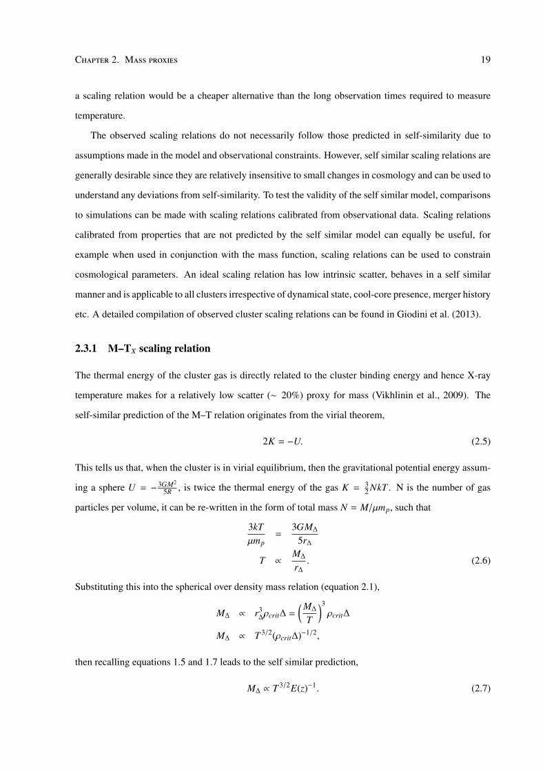
2.3.1 M–TX scaling relation

The thermal energy of the cluster gas is directly related to the cluster binding energy and hence X-ray

temperature makes for a relatively low scatter (∼ 20%) proxy for mass (Vikhlinin et al., 2009). The

self-similar prediction of the M–T relation originates from the virial theorem,

2K = −U. (2.5)

This tells us that, when the cluster is in virial equilibrium, then the gravitational potential energy assum-

ing a sphere U = − 3GM2

5R , is twice the thermal energy of the gas K = 32 NkT . N is the number of gas

particles per volume, it can be re-written in the form of total mass N = M/µmp, such that

3kTµmp

=3GM∆

5r∆

T ∝M∆

r∆

. (2.6)

Substituting this into the spherical over density mass relation (equation 2.1),

M∆ ∝ r3∆ρcrit∆ =

( M∆

T

)3ρcrit∆

M∆ ∝ T 3/2(ρcrit∆)−1/2,

then recalling equations 1.5 and 1.7 leads to the self similar prediction,

M∆ ∝ T 3/2E(z)−1. (2.7)


This means that for a given mass, objects at higher redshift will tend to be hotter systems than those at low

redshift. For massive clusters (> 3 keV), the observed hydrostatic mass – X-ray temperature relation is

in good agreement with the predicted slope of 3/2 (e.g. Sun et al., 2009; Vikhlinin et al., 2009; Eckmiller

et al., 2011; Jee et al., 2011), whereas samples that include groups sized systems are observed to have

much steeper slopes as high as ∼ 2 (Mohr et al., 1999; Finoguenov et al., 2001; O’Hara et al., 2007).

Simulations (Le Brun et al., 2014) find that the M–T scaling relation is the most robust against bary-

onic physics and feedback processes, however accurate temperature measurements require long exposure

times and cool core presence and dynamical state are known to affect the scatter on the derived relation

(Kravtsov et al., 2006).

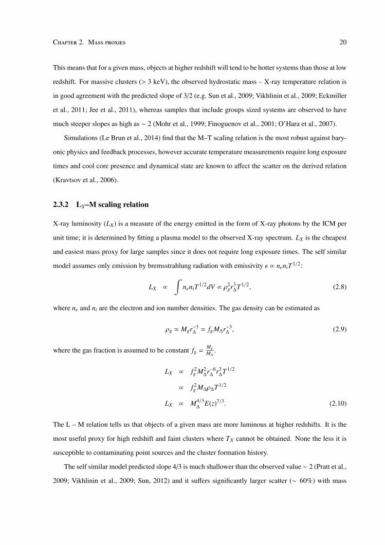
2.3.2 LX–M scaling relation

X-ray luminosity (LX) is a measure of the energy emitted in the form of X-ray photons by the ICM per

unit time; it is determined by fitting a plasma model to the observed X-ray spectrum. LX is the cheapest

and easiest mass proxy for large samples since it does not require long exposure times. The self similar

model assumes only emission by bremsstrahlung radiation with emissivity ε ∝ neniT 1/2:

LX ∝

∫neniT 1/2dV ∝ ρ2

gr3∆T 1/2, (2.8)

where ne and ni are the electron and ion number densities. The gas density can be estimated as

ρg ' Mgr−3∆ = fgM∆r−3

∆ , (2.9)

where the gas fraction is assumed to be constant fg =MgM∆

.

LX ∝ f 2g M2

∆r−6∆ r3

∆T 1/2

∝ f 2g M∆ρ∆T 1/2

LX ∝ M4/3∆

E(z)7/3. (2.10)

The L – M relation tells us that objects of a given mass are more luminous at higher redshifts. It is the

most useful proxy for high redshift and faint clusters where TX cannot be obtained. None the less it is

susceptible to contaminating point sources and the cluster formation history.

The self similar model predicted slope 4/3 is much shallower than the observed value ∼ 2 (Pratt et al.,

2009; Vikhlinin et al., 2009; Sun, 2012) and it suffers significantly larger scatter (∼ 60%) with mass


(Stanek et al., 2006) in comparison to temperature. The scatter is correlated to the cluster morphology,

with relaxed, cool core systems showing tighter scatter than relations of non-relaxed clusters. Scaling

relations that use core-excised temperature and luminosity also show smaller scatter values suggesting

that the thermal properties of the central gas play a important role (McCarthy et al., 2008).

Evidently from equation 2.9, the self-similar prediction of the gas mass – mass relation (Mg–M)

has a slope of 1. Gas mass is a low scatter mass proxy (∼ 15%, Mahdavi et al., 2013) subject to the

lower sensitivity to mergers however observations also indicate the possibility of a mass dependent slope

(Zhang et al., 2008).

2.3.3 Other scaling relations

For completeness, the L–T scaling relation predicted from the self similar model goes as LX ∝ T 2E(z)

with typical observational slopes being significantly steeper (O’Hara et al., 2007; Pratt et al., 2009;

Maughan et al., 2012). The observed scatter on luminosity in the L–T relation is also very high (∼ 70%),

mostly dominated by the presence of cool cores.

Other common scaling relations with mass include the YS Z–M relation (e.g. Bonamente et al., 2008;

Marrone et al., 2009), where YS Z is the integrated gas pressure along the line of sight observed with SZE

data. The SZE signal is independent of cluster redshift so is particularly useful to identify clusters out to

high redshifts.

The M–YX relation where YX is a product of the gas mass and cluster temperature has a predicted

slope of 3/5 (Kravtsov et al., 2006). In simulations, this relation has been shown to produce very small

scatter of 5-8% regardless of the dynamical state of the cluster sample, however observations indicate a

higher scatter of up to 20% (Okabe et al., 2010; Mahdavi et al., 2013). More recent simulations by Le

Brun et al. (2014) suggest that the M–YX relation is subject to baryonic effects that are more significant

in groups.

Lastly the near infrared (NIR) luminosity – mass relation, where NIR luminosity is related to the

stellar mass (M∗). In particular for K-band luminosity, observations suggest typically a ∼ 30% scatter

(e.g. Lin et al., 2003), however more recent work by Mulroy et al. (2014) who calibrate an LK–M relation

based on weak lensing masses show a significantly smaller scatter of ∼ 10% and a slope of ∼ 1, alluding

to evidence of a constant stellar mass to total mass ratio.


5x1013 1014 2x1014

1043

1044

M [Msol]

L X [e

rg/s

]

M [Msol]L X

[erg

/s]

1013 1014 1015

1042

1043

1044

1045

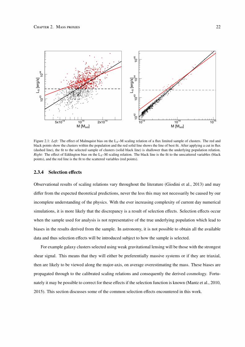
Figure 2.1: Left: The effect of Malmquist bias on the LX–M scaling relation of a flux limited sample of clusters. The red andblack points show the clusters within the population and the red solid line shows the line of best fit. After applying a cut in flux(dashed line), the fit to the selected sample of clusters (solid black line) is shallower than the underlying population relation.Right: The effect of Eddington bias on the LX–M scaling relation. The black line is the fit to the unscattered variables (blackpoints), and the red line is the fit to the scattered variables (red points).

2.3.4 Selection effects

Observational results of scaling relations vary throughout the literature (Giodini et al., 2013) and may

differ from the expected theoretical predictions, never the less this may not necessarily be caused by our

incomplete understanding of the physics. With the ever increasing complexity of current day numerical

simulations, it is more likely that the discrepancy is a result of selection effects. Selection effects occur

when the sample used for analysis is not representative of the true underlying population which lead to

biases in the results derived from the sample. In astronomy, it is not possible to obtain all the available

data and thus selection effects will be introduced subject to how the sample is selected.

For example galaxy clusters selected using weak gravitational lensing will be those with the strongest

shear signal. This means that they will either be preferentially massive systems or if they are triaxial,

then are likely to be viewed along the major-axis, on average overestimating the mass. These biases are

propagated through to the calibrated scaling relations and consequently the derived cosmology. Fortu-

nately it may be possible to correct for these effects if the selection function is known (Mantz et al., 2010,

2015). This section discusses some of the common selection effects encountered in this work.


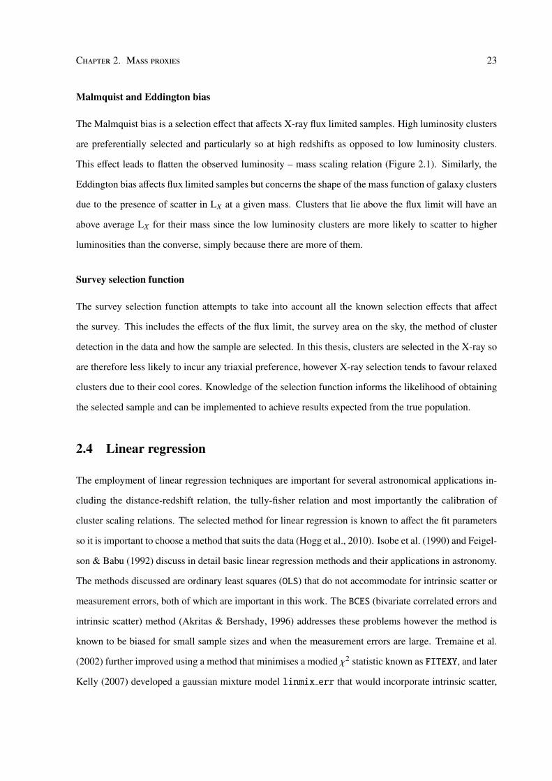
Malmquist and Eddington bias

The Malmquist bias is a selection effect that affects X-ray flux limited samples. High luminosity clusters

are preferentially selected and particularly so at high redshifts as opposed to low luminosity clusters.

This effect leads to flatten the observed luminosity – mass scaling relation (Figure 2.1). Similarly, the

Eddington bias affects flux limited samples but concerns the shape of the mass function of galaxy clusters

due to the presence of scatter in LX at a given mass. Clusters that lie above the flux limit will have an

above average LX for their mass since the low luminosity clusters are more likely to scatter to higher

luminosities than the converse, simply because there are more of them.

Survey selection function

The survey selection function attempts to take into account all the known selection effects that affect

the survey. This includes the effects of the flux limit, the survey area on the sky, the method of cluster

detection in the data and how the sample are selected. In this thesis, clusters are selected in the X-ray so

are therefore less likely to incur any triaxial preference, however X-ray selection tends to favour relaxed

clusters due to their cool cores. Knowledge of the selection function informs the likelihood of obtaining

the selected sample and can be implemented to achieve results expected from the true population.

2.4 Linear regression

The employment of linear regression techniques are important for several astronomical applications in-

cluding the distance-redshift relation, the tully-fisher relation and most importantly the calibration of

cluster scaling relations. The selected method for linear regression is known to affect the fit parameters

so it is important to choose a method that suits the data (Hogg et al., 2010). Isobe et al. (1990) and Feigel-

son & Babu (1992) discuss in detail basic linear regression methods and their applications in astronomy.

The methods discussed are ordinary least squares (OLS) that do not accommodate for intrinsic scatter or

measurement errors, both of which are important in this work. The BCES (bivariate correlated errors and

intrinsic scatter) method (Akritas & Bershady, 1996) addresses these problems however the method is

known to be biased for small sample sizes and when the measurement errors are large. Tremaine et al.

(2002) further improved using a method that minimises a modied χ2 statistic known as FITEXY, and later

Kelly (2007) developed a gaussian mixture model linmix err that would incorporate intrinsic scatter,


measurement errors, non-detections and selection effects. The following sections will discuss in more

detail the common fitting methods used in scaling relations in astronomy.

Assuming a bivariate data set xi, yi, i=1, 2, ... n, with a covariance matrix

Σ =

σ2x σxy

σxy σ2y

, (2.11)

where σx, σy, σxy are the measurement errors of x and y and their covariance respectively. The model is

assumed to have the form y = α + βx + σint, where α, β, σint are the normalisation, slope and intrinsic

scatter in y respectively. For independent variables, the measurement errors are uncorrelated and the

correlation coefficient ρ=0 in σxy.

2.4.1 BCES(Y|X)

The BCES(Y|X) estimator (Akritas & Bershady, 1996) is the most common in astronomy. It originates

from the OLS(Y|X) estimator that has a slope β that minimises the residuals in y, so β =cov(x,y)var(x) , however

also takes into account the measurement errors. The slope (β), intercept (α) and respective errors (σβ,

σα) are,

β =cov(x, y) − 〈σxy〉

var(x) − 〈σ2x〉

, (2.12)

α = 〈y〉 − β〈x〉, (2.13)

σ2β = n−1var(ξ), (2.14)

σ2α = n−1var(ζ). (2.15)

where

ξi =(xi − 〈x〉)(yi − βxi − α) + βΣ11,i − Σ12,i

var(x) − 〈σ2x〉

, (2.16)

ζi = yi − βxi − 〈x〉ξi, (2.17)

〈...〉 denotes the expectation value, cov(x, y) is the covariance of x and y, and var(x) is the variance of

x. Note that neglecting the measurement error terms reduces BCES(Y|X) to the formalism of OLS(Y|X).

The intrinsic scatter is

σint =

√var(y) − 〈σ2

y〉 − β(cov(x, y) − 〈σxy〉) (2.18)


The BCES(X|Y) minimises the residuals on the x variables. It has the same intercept as BCES(Y|X)

but the slope β and ξi is defined as

β =var(y) − 〈σ2

y〉

cov(x, y) − 〈σxy〉, (2.19)

ξi =(yi − 〈y〉)(yi − βxi − α) + βΣ12,i − Σ22,i

cov(x, y) − 〈σxy〉(2.20)

2.4.2 Bisector

Since the BCES(Y|X) and BCES(X|Y) methods give inconsistent slopes, the bisector method was intro-

duced to give a line that bisects the two. Parameters β and ξi are replaced by,

β =1

β1 + β2

[β1β2 − 1 +

√(1 + β2

1)(1 + β22)]

(2.21)

ξi =(1 + β2

2)βξ1,i

(β1 + β2)√

(1 + β21)(1 + β2

2)+

(1 + β21)βξ2,i

(β1 + β2)√

(1 + β21)(1 + β2

2)(2.22)

where β1, β2 are the slopes in equations 2.12 and 2.19 respectively.

2.4.3 Orthogonal

The BCES(Orthogonal) estimator minimises the orthogonal distances from the line of best fit.

β =12

[(β2 − β

−11 ) + sgn(cov(x, y))

√4 + (β2 − β

−11 )2

](2.23)

ξi =βξ1,i

β21

√4 + (β2 − β

−11 )2

+βξ2,i√

4 + (β2 − β−11 )2

(2.24)

Both the bisector and orthogonal methods are symmetric, and either method can be used when it is

unclear which variable should be treated as the dependent and which the independent.

2.4.4 MPFITEXY

MPFITEXY is similar to routine to FITEXY that uses the Levenberg-Marquardt technique (MPFIT, Mark-

wardt (2009)) to minimise the non-linear least squares to model linear regression (Williams et al., 2010)

χ2 =

n∑i=0

(y − βx − α)2

σ2y + β2σ2

x + σ2int

(2.25)

The uncertainties on the regression parameters are computed from the covariance matrix. The intrinsic

scatter is obtained iteratively to ensure that the reduced chi square χ2red = χ2

min/d.o. f ≈ 1, which in this


case d.o. f = n−2. When χ2red < 1, the intrinsic scatter is set to σint = 0 and similarly the uncertainties on

the regression parameters are meaningless unless χred = 1, since it implies that either the observational

uncertainties or the intrinsic scatter is not well estimated. The total scatter is

σ2tot =

χ2min∑n

i=0(σ2y + β2σ2

x + σ2int)−1. (2.26)

2.4.5 linmix err

Kelly (2007) show that the least square estimate of the slope when data with measurement error is biased

with respect to data without measurement error. They develop a bayesian method (linmix err) that

is particularly attractive to the astronomical community since it accommodates both for non-detections

(Isobe et al., 1986), where data do not have a measured error, and selection effects (as discussed section

2.3.4) such as the malmquist bias. The distribution of the observed data zi = yi, xi is modelled as a

mixture of K gaussian functions that are described by their weight π = π1, ...πK (note that∑K

k=1 πk = 1),

mean µ = µ1, ...µK and variance τ2 = τ1, ...τK The likelihood function of the observed data is

p(x, y|θ,φ) =

n∏i=1

K∑k=1

πk

2π|Vk,i|1/2 exp

[−

12

(zi − ζk)ᵀV−1k,i (zi − ζk)

], (2.27)

ζk =

α + βµk

µk

(2.28)

Vk,i =

β2τ2

k + σ2int + σ2

y,i βτ2k + σxy,i

βτ2k + σxy,i τ2

k + σ2x,i

(2.29)

where θ = α, β, σ2int, φ = π,µ, τ2. The code samples the posterior using either Gibbs Sampling or

Metropolis-Hastings MCMC methods (see section 3.1.1). This method treats the problem as a fixed effect

(Gelman et al., 2014) such that the gaussian functions are modelled on the x variable as the predictor for

y, the response variable. The intrinsic scatter is assumed to exist only on the response variable. Later on

(Chapter 7), a similar method is developed to obtain linear regression parameters however it is much less

restrictive since the components of the covariance matrix is sampled for.

Park et al. (2012) show that the BCES estimators work well only in the cases of small measurement

errors. They find MPFITEXY to be the best estimator compared to the other methods and is less computa-

tionally exhaustive than linmix err, however the latter produces the full posterior distribution function.


2.4.6 Error estimation

The two most common methods for error estimation are jack knife resampling and bootstrap resampling.

Jack knife resampling is used to estimate the variance of the sample mean by making copies of the

original data set whilst emitting each data point from the sample. The mean of each resampled data set

is then used to calculate the error on the mean of the original data.

Bootstrap resampling can be used to estimate the distribution of the sample mean x by resampling

the distribution of x with replacement to obtain multiple variations of the initial sample. For example a

resampled distribution could be x2, x6, x4, x4, x4, x1, x2. Taking the mean of each of the resampled data

sets, gives a distribution of x values that can be used to estimate the error on the true sample mean for

example by taking the standard deviation.

2.5 Summary

This chapter introduced cluster mass measurement and cluster scaling relations which are a prominent

feature in this thesis. I have described the self similar theoretical model where cluster scaling relations

are governed by gravity only and compared them with current observations. I have also discussed some

of the effects that plague observational results and some of the popular linear regression methods to fit

scaling relations.

Although most clusters are detected in the X-ray, the assumptions required make it a less favoured

mass estimator in comparison to weak gravitational lensing mass which only depends on the underly-

ing mass distribution. Towards the low mass of groups, the estimation of mass becomes increasingly

difficult. In the X-ray, count rate is smaller and the susceptibility to AGN contamination increases and

in gravitational lensing the limitations are due to low signal-to-noise. Many studies have shown dis-

crepancies between lensing and X-ray based mass measurements (Miralda-Escude & Babul, 1995) and

many attempts have been made to reconcile this so called hydrostatic mass bias (Smith et al., 2016).

Observations suggest a bias of around 10% but increasing for lower mass halos (Kettula et al., 2013).

Whether or not this bias is real or due to gaps in our understanding of cluster physics is ongoing research

and will benefit greatly from simulations which has only recently been extended to include baryonic

physics (e.g. Le Brun et al., 2014; Pike et al., 2014). The current status of cluster mass measurement is

that discrepancies exist in mass estimates arising from the method used, and discrepancies exist between


various studies of cluster scaling relations likely due to selection effects. This highlights the importance

of using scaling relations that are derived from samples with properties similar to the sample of interest

but also that these discrepancies need to be fully understood before we can properly excise clusters for

cosmological measurements.

Chapter 3

Bayesian inference

Bayesian inference is becoming more widely used to analyse astronomical data. In this regime, incor-

porating prior information enables better constraints on the predicted outcomes. This chapter gives an

introduction to the statistical techniques relied upon in the next few chapters of this thesis, all of which

can be found in any good bayesian statistics book (e.g. Gelman et al., 2014).

3.1 The Bayesics

In frequentist statistics, the probability of an event occurring can be be measured from the frequency

it occurs. In Astronomy however this is not always very helpful since it may be not be possible to

repeat observations - for example, is the case of supernovae explosions. Bayesian statistics treat the

probability of an event occurring as a degree of belief given the evidence available and is updated as

more information is attained. Bayes’ Theorem is the fundamental equation in Bayesian statistics and

can be easily derived from the conditional probability equation. The joint probability of events A and B

occurring is the product of the probability of event A occurring given B has occurred and the probability

of event B occurring:

P(A, B) = P(A|B)P(B) = P(B, A) = P(B|A)P(A), (3.1)

rearranging this gives Bayes′ theorem

P(M|D, I) =P(D|M, I)P(M|I)

P(D|I). (3.2)

Here, M is the model or hypothesis of the parameter(s), D is the data and I is the prior information (which

can be ignored in the equation). P(M|D, I) is called the posterior density function (PDF) and is a measure

of our state of knowledge of M. The PDF covers a range of M values, but should also encompass the true

value of M. Preferably when presenting the result it is optimal to provide the PDF, but when this is not

possible, summary statistics that best describe the distribution will suffice. P(D|M, I) is the likelihood

29

Chapter 3. Bayesian inference 30

which in this case is measure of how well the model fits the data. As more data is obtained the likelihood

narrows and the influence of the prior becomes negligible. P(M|I) is the prior, it incorporates any prior

information we know about the model and lastly P(D|I) is the marginal likelihood or evidence. This

normalising constant ensures that the probabilities sum to 1 and is important for model comparison but

not in this work so can be ignored.

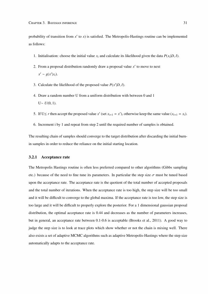
3.1.1 Markov Chain Monte Carlo

Bayes’ equation can be used to determine the probability of a model given the data whilst incorporating

any prior information. However, suppose that there are 2 parameters in the model that are of interest

and they are continuous variables. The PDF therefore lives on a 2 dimensional parameter space which

can be gridded up infinitesimally and the calculation of P(D|MI) at every grid pixel would be extremely

computationally expensive. Markov Chain Monte Carlo (MCMC) are algorithms that offer a simple

and efficient way to sample from the posterior distribution. A Markov chain is a path in the parameter

space where the PDF is evaluated. Each step in the parameter space is solely dependent on the previous

location. As the steps reach an equilibrium state, it converges to the target posterior distribution.

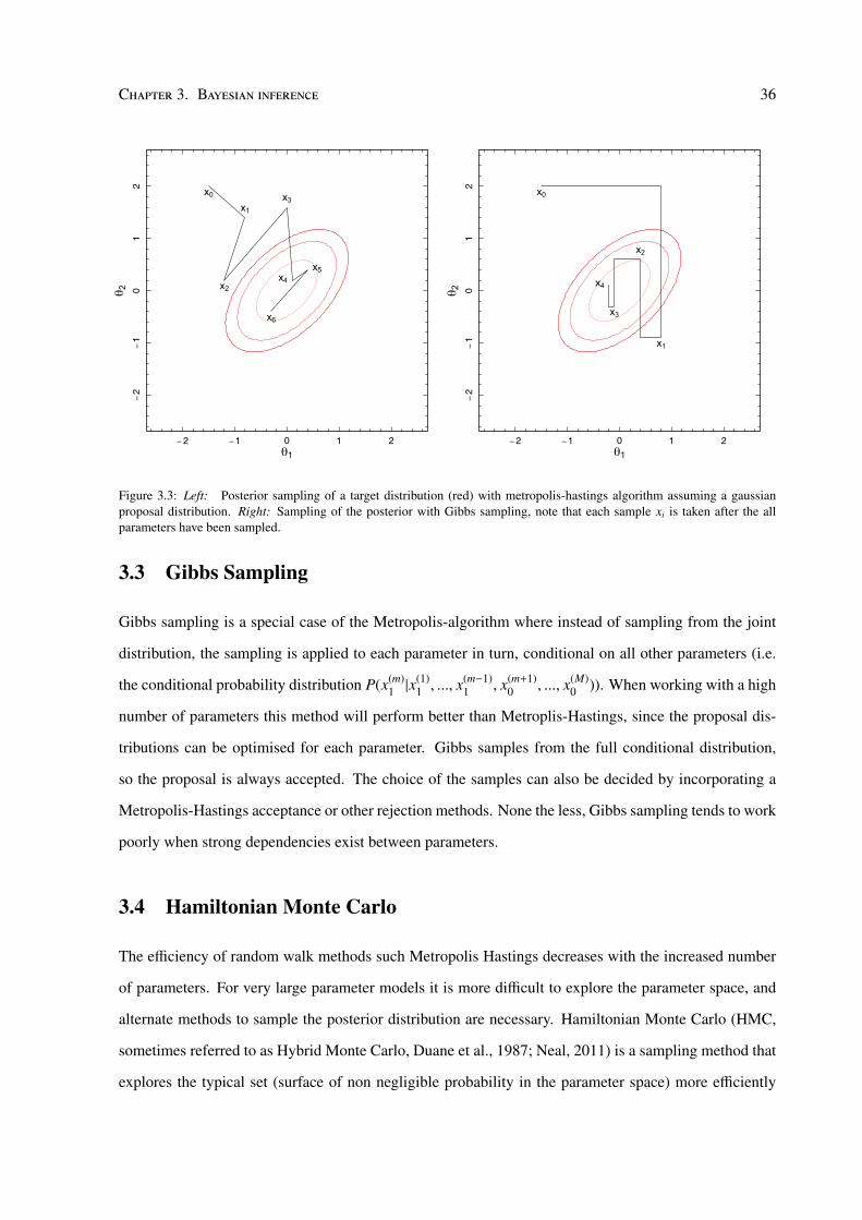
3.2 The Metropolis Hastings algorithm

The Metropolis-Hastings algorithm is an implementation of MCMC. It is a random walk in which a

proposal step (x′) is made based upon some proposal distribution g(x′|x). This proposal step is dependent

on only the current location in the parameter space and the step size and is commonly taken as a gaussian

(or multivariate gaussian) distribution with mean x and standard deviation σ. The acceptance of the

proposed step depends on the acceptance distribution

A(x′|x) = min(1, r) = min(1,

P(x′|D, I)g(x|x′)P(x|D, I)g(x|x′)

), (3.3)

where r is the metropolis ratio and gives the probability of acceptance. If r ≥ 1 then the step is always

accepted, otherwise it is accepted with a probability r. This helps to prevent the chain getting stuck

at local maxima. Note that r is not simply the ratio of the likelihoods P(x′ |D,I)P(x|D,I) but multiplied by the

ratio of proposal distributions. For symmetric proposal distributions g(x|x′) = g(x′|x). Including this

ratio ensures that the detailed balance condition (the probability of transition from x to x′ is equal to the


probability of transition from x′ to x) is satisfied. The Metropolis-Hastings routine can be implemented

as follows:

1. Initialisation: choose the initial value xi and calculate its likelihood given the data P(xi|D, I).

2. From a proposal distribution randomly draw a proposal value x′ to move to next

x′ ∼ g(x′|xi).

3. Calculate the likelihood of the proposed value P(x′|D, I).

4. Draw a random number U from a uniform distribution with between 0 and 1

U∼ U(0, 1).

5. If U≤ r then accept the proposed value x′ (set xi+1 = x′), otherwise keep the same value (xi+1 = xi).

6. Increment i by 1 and repeat from step 2 until the required number of samples is obtained.

The resulting chain of samples should converge to the target distribution after discarding the initial burn-

in samples in order to reduce the reliance on the initial starting location.

3.2.1 Acceptance rate

The Metropolis Hastings routine is often less preferred compared to other algorithms (Gibbs sampling

etc.) because of the need to fine tune its parameters. In particular the step size σ must be tuned based

upon the acceptance rate. The acceptance rate is the quotient of the total number of accepted proposals

and the total number of iterations. When the acceptance rate is too high, the step size will be too small

and it will be difficult to converge to the global maxima. If the acceptance rate is too low, the step size is

too large and it will be difficult to properly explore the posterior. For a 1 dimensional gaussian proposal

distribution, the optimal acceptance rate is 0.44 and decreases as the number of parameters increases,

but in general, an acceptance rate between 0.1-0.6 is acceptable (Brooks et al., 2011). A good way to

judge the step size is to look at trace plots which show whether or not the chain is mixing well. There

also exists a set of adaptive MCMC algorithms such as adaptive Metropolis-Hastings where the step size

automatically adapts to the acceptance rate.


0.1 1 10

00.2

0.4

0.6

0.8

1

x

P(x)

UniformJeffreys

0.1 1 10

00.2

0.4

0.6

0.8

1

xP

(ln x

) = x

P(x

)

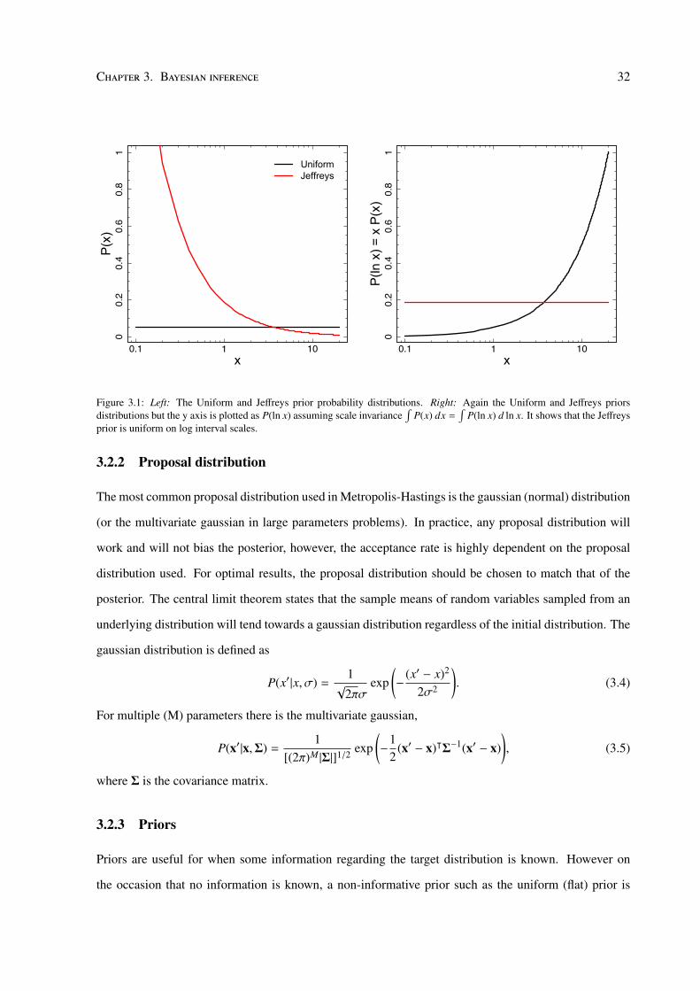
Figure 3.1: Left: The Uniform and Jeffreys prior probability distributions. Right: Again the Uniform and Jeffreys priorsdistributions but the y axis is plotted as P(ln x) assuming scale invariance

∫P(x) dx =

∫P(ln x) d ln x. It shows that the Jeffreys

prior is uniform on log interval scales.

3.2.2 Proposal distribution

The most common proposal distribution used in Metropolis-Hastings is the gaussian (normal) distribution

(or the multivariate gaussian in large parameters problems). In practice, any proposal distribution will

work and will not bias the posterior, however, the acceptance rate is highly dependent on the proposal

distribution used. For optimal results, the proposal distribution should be chosen to match that of the

posterior. The central limit theorem states that the sample means of random variables sampled from an

underlying distribution will tend towards a gaussian distribution regardless of the initial distribution. The

gaussian distribution is defined as

P(x′|x, σ) =1√

2πσexp

(−

(x′ − x)2

2σ2

). (3.4)

For multiple (M) parameters there is the multivariate gaussian,

P(x′|x,Σ) =1

[(2π)M |Σ|]1/2 exp(−

12

(x′ − x)ᵀΣ−1(x′ − x)), (3.5)

where Σ is the covariance matrix.

3.2.3 Priors

Priors are useful for when some information regarding the target distribution is known. However on

the occasion that no information is known, a non-informative prior such as the uniform (flat) prior is


required. Since it is not computationally feasible to sample from all parameter values (−∞ → ∞), the

uniform prior is typically taken as a top-hat function with limits at the edges of the parameter space. This

is given by

P(x) =1

xmax − xmin(3.6)

i.e it gives uniform probability to all values of x in the range limit.

This prior works well when the range of parameters is small, however in astronomy the quantities

of interest generally span large orders of magnitude. For example the mass range of galaxy groups and

clusters is 1013−1015 M. Using a uniform prior to sample this parameter space would induce a bias. To

demonstrate this, take for example the comparison of the probability that x lies between 1013 − 1014 M

and the probability that x lies between 1014 − 1015 M∫ 1014

1013 P(x) dx∫ 1015

1014 P(x) dx= 0.1. (3.7)

This means that it is 10 times more favoured for x to lie between 1014 − 1015 M when using a uniform

prior. It would therefore be more appropriate to use a scale invariant prior such as Jeffreys prior where

the prior is flat on a logarithmic scale (Fig. 3.1)

P(x) =1

x ln(xmax/xmin). (3.8)

Note that the Jeffreys prior diverges at x = 0, in which case an alternative prior must be used such as the

modified Jeffreys prior. When more information about the scale of the parameter of interest is available,

it might be preferable to instead use a weakly informative prior. Commonly a gaussian function prior

is used with a large variance however in some cases this too may be too restrictive to accommodate for

outliers. In which case a Cauchy distribution prior, effectively a gaussian with infinite tails, would be

more appropriate.

3.2.4 Convergence

MCMC is ergodic. Every location in the parameter space is eventually reachable from any other location

in the parameter space in a finite number of steps. The distribution of samples in the MCMC chain will

trace the target posterior distribution once the chain has been run long enough to attain a sufficient number

of samples. The chain is said to have converged, once this stationary distribution is achieved, however


0 200 400 600 800 1000

9.5

1010.5

11θ

0 200 400 600 800 1000iteration

0 200 400 600 800 1000

Figure 3.2: Traceplots of an MCMC sample, left is an example of a chain that has good mixing. Middle shows moderate mixing,the samples fluctuate about the convergence value, however the steps are small so will require a lot of thinning to remove thecorrelation between samples. Right is an example of bad mixing, the samples do not converge.

the samples in the chain correlated, which may lead to a false impression that the chain has converged.

In order to reduce the problem, the chain can be thinned by first computing the autocorrelation function

A(L) = A(−L) =

∑N−L−1k=0 (xk − x)(xk+L − x)∑N−1

k=0 (xk − x)2, (3.9)

where L is the lag, N is the total number of samples, xk is the kth sample in the chain and x is the

sample mean. Plotting the autocorrelation function against lag reveals how much the shift must be

applied between the samples before the samples in the chain are independent. This is the autocorrelation

length. Taking samples in the chain separated by the autocorrelation length (thinning the chain) ensures

uncorrelated samples.

Their are a number of ways to test whether the chain has converged (Cowles & Carlin, 1996). One

method is to run multiple MCMC chains initiating in different locations of the parameter space and test

that they all converge to the same posterior. The Gelman-Rubin convergence criterion (Gelman & Rubin,

1992) is a diagnostic that compares the variance within each chain to the variance between chains,

R =(1 − 1

N ) + J+1J2−J

∑Jj=1(x j − x)2

1J(N−1)

∑Nn=1

∑Jj=1(x j

n − x j)2, (3.10)

where N is the number of samples, J is the number of chains, x j is the mean of the jth chain, x is the

mean of all the chains combined and x jn is the nth sample in the jth chain. As convergence is reached, R

will approach unity. Generally a chain is converged if R < 1.03.

Another convergence diagnostic is to visually inspect the traceplot (Figure 3.2), a plot of each sample

drawn at each time step. An ideal trace plot will show good mixing, fluctuating uniformly about the

convergence value. With trace plots it is easy to identify steps in the chain being too small and hence

highly correlated samples, as well as those that don’t converge at all (bad mixing).


3.2.5 Summary statistics

In Bayesian statistics the result of the analysis should be reported as the full posterior probability density

as this contains the complete information. The frequentist (and also most common) approach is to report

a point estimate and it’s reliability. One way to decide the summary statistic that communicates the

largest amount of information, is to calculate the expected posterior loss of the point estimate x and to

minimise it. This is the loss function.

E(x) =

∫L(x, x)P(x|D)dx (3.11)

The maximum a posteriori (MAP) estimate is the mode of the posterior. It is particularly useful for

multimodal posteriors, where highest modal estimate(s) are useful. Note however the the mode of a

joint posterior P(x1, x2|D) does not necessarily correspond to the mode of the marginalised posteriors

P(x1|D), P(x2|D). When the loss function L(x, x) is zero-one, then the Bayes estimator is the mode, how-

ever for continuous distributions this loss function is invalid. The median is the optimal Bayes’ estimator

when the loss function is linear. It is generally invariant under re-parameterisation i.e. the median of

P(x) = the median of log(P(x)), however although it is unambiguous to define the median of a univariate

distribution, the median of a multivariate distribution less trivial. In high dimensional problems the mean

is the optimal estimator to trace the posterior mass because as the number of parameters increases the

area surrounding the modal peak becomes less important. The mean is the Bayes estimator for quadratic

loss functions. It is relatively invariant under rescaling however there are cases where the mean is non-

physical for example when it lies between 2 peaks in a region of 0 probability, or a cauchy disturbution

that tails off to infinity. It is also important to give a statistic that conveys the reliability of the point

estimate. Commonly this is the standard deviation which is related to the spread of the distribution or the

confidence interval where one can say with some percentage of confidence that the true value lies with

that interval. For multimodal or high dimensional problems, the credible interval (or credible region)

should be used. This grids up the posterior, counting from the highest density regions until some per-

centage of the total is reached. The density of the posterior is proportional to the likelihood, with 1,2, and

3 σ credible intervals corresponding to 68, 95 and 99.7% of the posterior mass. Credible intervals are

favourable over the other measures of reliability discussed as it is not limited to gaussian distributions.

Chapter 3. Bayesian inference 36θ 2

θ1−2 −1 0 1 2

−2

−1

01

2 x0x1

x2

x3

x4x5

x6

θ 2θ1

−2 −1 0 1 2

−2

−1

01

2 x0

x1

x2

x3

x4

Figure 3.3: Left: Posterior sampling of a target distribution (red) with metropolis-hastings algorithm assuming a gaussianproposal distribution. Right: Sampling of the posterior with Gibbs sampling, note that each sample xi is taken after the allparameters have been sampled.

3.3 Gibbs Sampling

Gibbs sampling is a special case of the Metropolis-algorithm where instead of sampling from the joint

distribution, the sampling is applied to each parameter in turn, conditional on all other parameters (i.e.

the conditional probability distribution P(x(m)1 |x

(1)1 , ..., x(m−1)

1 , x(m+1)0 , ..., x(M)

0 )). When working with a high

number of parameters this method will perform better than Metroplis-Hastings, since the proposal dis-

tributions can be optimised for each parameter. Gibbs samples from the full conditional distribution,

so the proposal is always accepted. The choice of the samples can also be decided by incorporating a

Metropolis-Hastings acceptance or other rejection methods. None the less, Gibbs sampling tends to work

poorly when strong dependencies exist between parameters.

3.4 Hamiltonian Monte Carlo

The efficiency of random walk methods such Metropolis Hastings decreases with the increased number

of parameters. For very large parameter models it is more difficult to explore the parameter space, and

alternate methods to sample the posterior distribution are necessary. Hamiltonian Monte Carlo (HMC,

sometimes referred to as Hybrid Monte Carlo, Duane et al., 1987; Neal, 2011) is a sampling method that

explores the typical set (surface of non negligible probability in the parameter space) more efficiently


by using the gradient of the log posterior and hamiltonian dynamics. In previous sampling routines,

for a given set of parameters θ and data y, the object of interest was the posterior P(θ|y). In HMC

the npar dimensional parameter space is transformed into a 2npar dimensional phase space, where each

parameter corresponds to a fictitious particle with co-ordinate θi and an assigned random momentum ui.

The sampling occurs on the joint density also known as the extended target density,

P(u, θ) = P(u|θ)P(θ) (3.12)

= exp[−H(θ, u)]. (3.13)

The Hamiltonian is defined as the sum of kinetic and potential energy terms, H(θ, u) = K(u|θ) + U(θ),

where the particle kinetic energy is

K(u|θ) = − ln P(u|θ) =uᵀu2, (3.14)

and the potential energy is governed by the log posterior

U(θ) = − ln P(θ). (3.15)

The momenta u is eventually marginalised out to obtain the target posterior. The system evolves accord-

ing to the Hamiltonian equations

dθdt

=∂H∂u

=∂K∂u

= u (3.16)

dudt

= −∂H∂θ

= −∂U∂θ

(3.17)

Since H is constant, the extended target density is uniform and hence the acceptance rate is 1. This allows

efficient exploration of the parameter space, and the generation of new random values of ui enables large

steps. However U(θ) is unknown, it is the quantity that we are seeking and can either be approximated

by running a short MCMC or by computing the derivative.

To solve the differential equations, a leapfrog algorithm is usually implemented as follows

1. Draw the particle momentum randomly from a normal distribution u ∼ N(0, 1)

2. Update the momentum by half a time step and update the position by a full time step (or step size,

ε) based on the new momentum value

u ← u −ε

2∂U∂θ

(3.18)

θ ← θ + εu (3.19)


3. Update the momentum by the remaining half a time step

u← u −ε

2∂U∂θ

(3.20)

4. Since U is an approximation, H is not exactly constant and a metropolis-hastings acceptance dis-

tribution is needed to decide on the acceptance of the sample and to ensure detailed balance.

A(θ′, u′|θ, u) = min(1, exp(H(θ, u) − H(θ′, u′))). (3.21)

5. If the proposal state is not accepted, then the existing state is added to sample and the algorithm is

iterated over the current state until the required number of steps is achieved.

The sampling efficiency of HMC is dependent on the tuning of 2 parameters, the step size ε and the

number of steps L. If ε is too small, the computational time will be very long, but if ε is too large, the

leapfrog integrator will be inaccurate resulting in many rejections. If L is too small, the samples will

exhibit random-walk like behaviour, but if L is too large the trajectories may loop back ending close to

the previous position, so again would be computationally exhaustive. Tuning these parameters by hand

would require computationally expensive preliminary runs. The No-U-turn sampler (NUTS Homan &

Gelman, 2014) is an adaptive HMC method that optimises these tuning parameters. For L the sampler

recursively doubles the number of steps until the point where a further increase in the number of steps

would no longer increase the distance between the proposal position θ′ and the initial position θ. This is

determined by the criterionddt

(θ′ − θ) · (θ′ − θ)2

≡ (θ′ − θ) · u′ < 0 (3.22)

i.e. the simulations are run until the proposal starts to make a U-turn and loop back on itself back

towards the initial position. This does not however guarantee time reversibility so in order to obey

detailed balance, the evolution of the Hamiltonian equations in NUTS runs both forwards and backwards

in time. This runs until either the criterion above is met or the maximum tree depth (maximum number

of doubling of ε) is reached and then slice sampling is used to decide on the final samples instead of the

metropolis acceptance ratio.

In order to automatically tune the step size ε, NUTS adopts a technique known as dual averaging

(Nesterov, 2009; Homan & Gelman, 2014) to obtain a particular average Metropolis acceptance ratio. For

HMC, the optimal value of ε corresponds to a theoretical acceptance ratio of 0.65. For high dimensions,


the acceptance ratio is closer to 0.85 Neal (2011). The larger the acceptance ratio, the smaller the step

size.

Both HMC and NUTS are rotation invariant which allows them to sample effectively from multivari-

ate densities with high correlations.

3.5 Summary

In this chapter I have provided a brief overview of the bayesian statistics starting from Bayes’ theorem.

I have introduced MCMC, an importance sampling method that can efficiently explore the posterior

distribution and provided examples of such routines used in this thesis, namely Metropolis-Hastings,

Gibbs sampling and Hamiltonian Monte Carlo. The importance of the choice of priors and posterior

distributions have been discussed as well as tests that the sampled chain has converged. Ideally the

results of importance sampling should be presented as the posterior distribution however sometimes this

is not possible. I have discussed some summary statistics that can be used to describe the posterior.

Statistical methods become increasingly important with the increasingly noisy astronomical data at high

redshifts. In order to extract the maximum amount of information and with the approaching launches of

future wide surveys, new statistical techniques need to be developed to prepare for the era of big data.

This chapter is the foundation of the analysis carried out in the following chapters.

Chapter 4

Weak gravitational lensing

In this chapter I discuss the basics of gravitational lens theory. This chapter introduces the formalism

for the analysis of the data used in chapters 6 and 7. The focus of this chapter is on Weak gravitational

lensing which isn’t without it’s limitations, for example; the weak lensing approximation that breaks

down near the cluster centre and the difficulty of accurate background galaxy selection. I also discuss

some of the other effects coming from the large scale structure. For further reviews on gravitational

lensing in clusters, I would suggest Narayan & Bartelmann (1996); Bartelmann & Schneider (2001);

Wittman (2002); Schneider et al. (2006).

4.1 The lens equation

As a light ray propagates through the gravitational field Φ of a lens, the effect of the space time curvature

can be expressed in terms of a refractive index

n = 1 −2c2 Φ, (4.1)

where c is the speed of light in a vacuum and assuming that the lens is a point mass M, it will have a

Newtonian potential of

Φ = −GM

(r2 + z2)1/2 , (4.2)

where the impact parameter r is the distance of closest approach and z is the adjacent distance from the

point mass. The angle of deflection is the integral of the gradient of n perpendicular to the direction of

40

Chapter 4. Weak gravitational lensing 41

Figure 4.1: A schematic diagram of a typical gravitational lens system.

travel

α = −

∫ ∞

−∞

∇⊥n dz = −2c2

∫∇⊥Φ dz

=4GM

c2

∫ ∞

0

z(r2 + z2)3/2 dz

=4GM

c2

[−

1(r2 + z2)1/2

]∞0

=4GMc2r

. (4.3)

For a gravitational lens system (Figure 4.1), an observer sees a source separated by an angle β from

the lens on the sky, however it is deflected by the gravitational potential of the lens and appears to be an

angle θ from the lens. Assuming that both the lens and source lie on planes perpendicular to the line of

sight to the lens with angular diameter distances Dl an Ds respectively, from geometry it can be seen that

θDs = βDs + αDls, (4.4)

where Dls is the distance between the source and lens. Note that Dls , Ds − Dl, for a spatially flat

Universe (Ωκ = 0) (Hogg, 1999),

Dls =Ds(1 + zs) − Dl(1 + zl)

1 + zs. (4.5)

Equation 4.4 can be rewritten to obtain the lens equation

β = θ − α (4.6)


where α =DlsDsα is the reduced deflection angle. The distances of the observer, lens and sources are

typically significantly larger than the size of the lens, which allows the lens to be approximated as a

plane. The distribution of its mass is characterised by its surface mass density, a measure of the projected

mass along the line of sight

Σ =

∫ρ dz (4.7)

For a lens with a constant surface mass density (i.e. Σ(r) = Σ),

α =Dls

Ds

4GMc2r

(4.8)

=4GDls

c2Ds r

∫ r

02πr′Σ dr′ (4.9)

=4GDls

c2Ds rΣπr2 (4.10)

=4πGΣθ

c2

DlsDl

Ds(4.11)

where θ = r/Dl. The density threshold required for strong lensing occurs at θ = α, where the source,

lens and observer are all aligned and the critical surface mass density is then defined as Σ(θ = α),

Σcrit =c2Ds

4πGDlDls. (4.12)

If Σ > Σcrit, then strong gravitational lensing effects are produced such as multiple images and caustics.

4.2 Shear and ellipticity

The Jacobian is a distortion matrix that maps light from the source plane (β) onto where we observe it

in the image plane (θ). It is given by the differential of the lensing equation

A =∂β

∂θ(4.13)

=∂

∂θ

(θ −

Dls

Dsα

)(4.14)

=∂

∂θ

(θ −

Dls

Ds

2c2

∫∇⊥Φ dz

)(4.15)

= δi j −∂2ψ

∂θi∂θ j(4.16)

where δi j is the kronecker delta function and ψ =DlsDl

Ds2c2

∫Φ dz is the effective lensing potential. Grav-

itational lensing causes both a distortion in the apparent size and apparent shape of objects that can be


parameterised by convergence κ and shear γ respectively. Both of these quantities can be expressed in

terms of the effective potential and κ is also conveniently expressed in terms of the surface mass density,

κ(θ) =12∇2ψ =

12

(ψ11 + ψ22), (4.17)

=Σ(θ)Σcrit

. (4.18)

where ψi j =∂2ψ∂θi∂θ j

. In order for shear to be expressed on a 2-D axis (γ1, γ2) with an orientation angle

φ measured anti-clockwise with respect to the x-axis (Figure 4.2), it must be decomposed in terms of a

complex quantity γ = γ1 + iγ2, where

γ1 = |γ| cos(2φ) =12

(ψ11 − ψ22), (4.19)

γ2 = |γ| sin(2φ) = ψ12 = ψ21. (4.20)

Consequently |γ| =√γ2

1 + γ22 and therefore the Lensing Jacobian can be written as,

A =

1 − ψ11 −ψ12

−ψ21 1 − ψ22

=

1 − κ − γ1 −γ2

−γ2 1 − κ + γ1

(4.21)

= (1 − κ)

1 0

0 1

− |γ| cos(2φ) sin(2φ)

sin(2φ) − cos(2φ)

(4.22)

In astronomy the background sources of interest are galaxies. The shape of a galaxy can be approxi-

mated as an ellipse with major (a) and minor (b) axes expressed as an ellipticity (Figure 4.2)

ε = ε1 + iε2 =a − ba + b

e2iφ. (4.23)

Galaxies are intrinsically elliptical and have random orientations so an ensemble average over a large

number of galaxies is required to measure the effects of gravitational lensing. In the weak lensing limit

(κ << 1), ellipticity is related to to shear in the following way

〈ε〉 = 〈g〉 =

⟨γ

1 − κ

⟩(4.24)

where g is the reduced shear that allows the decomposition of ellipticity into the intrinsic value εs and

that induced by lensing, g ' ε − εs. When averaging over a sufficient number of galaxy ellipticity values,

〈εs〉 = 0.

Note that g is invariant when the transformationA is scaled by some arbitrary scalar λ (i.e. γ′ = λγ),

whereas κ is not (1 − κ′ = λ(1 − κ)). Therefore κ can can only be determined up to transformation


−0.5 0 0.5

−0.5

00.5

e1e 2

Figure 4.2: Left: An illustration of the orientation angle φ and the semi-major a and minor b axes of a galaxy. Right: Variouscombinations of ellipticity components and the resulting galaxy shape.

κ′ = λκ + (1 − λ); this is a limitation of reconstructing the mass distribution and is known as mass sheet

degeneracy. Magnification (µ) is another consequence of gravitational lensing and is given as the inverse

determinant of the Jacobian, (µ = detA−1). If µ can be determined independently from shear, then it can

be used to break the degeneracy since µ′ = µλ−2.

4.2.1 Tangential shear

For weak lensing around galaxy groups and clusters, the measure of concern is the tangential shear γ+

(or tangential ellipticity ε+) because distortion due the mass of the galaxy cluster induces a tangential

alignment of background galaxies with respect to the cluster centre (Figure 4.3).

ε+ε× =

−<(εe−2iθ

)−=

(εe−2iθ

) =

− cos(2θ) − sin(2θ)

sin(2θ) − cos(2θ)

ε1

ε2

, (4.25)

where θ is the galaxy position angle. If the detected signal arises from gravitational lensing then any

signal should disappear when ellipticities are rotated by 45, therefore the cross component of ellipticity

ε× (equivalent to ε+ rotated by 45) can be used as a test for systematics (ideally 〈ε×〉 = 0). Another test

of systematics is to check that 〈ε+〉 = 0 when ellipticity values are randomised.


Figure 4.3: An illustration of the tangential and cross ellipticity of galaxy sources at different locations with respect to a centrepoint. The components of the ellipticity are assumed to be ε1 = 0.7 and ε2 = 0 for all 3 galaxies however the tangential andcross components of the ellipticity are dependent on the position angle θ.

4.2.2 Shape measurement

The intrinsic shape of a galaxy is not only affected by shear but also affected by atmospheric seeing,

instrumental effects from the telescope and detector and noise. These effects act to blur and pixelise the

observed shape of a galaxy causing distortions an order of magnitude larger than the lensing signal. In

principle the blurring can be easily predicted with the point spread function (PSF, which can be deter-

mined from calibration using stars assuming they are point sources), however in practice there are many

other influencing factors that are less trivial to model. Galaxies that form close together may be mutually

aligned due to the tidal force between them and galaxies that are in falling into dark matter halos are likely

to be aligned in the direction of infall (Sifon et al., 2015). These intrinsic alignments and other effects

such as the variation of the PSF with wavelength and location, contaminates the weak lensing signal. In

the case of ground based observations, simply building telescopes away from sea-level, at high-altitude,

dry locations can significantly improve seeing conditions and reduce atmospheric distortions.

Weak lensing is anticipated to be the most powerful technique to study dark energy when systematics

can be adequately controlled (Albrecht et al., 2006; Peacock et al., 2006; Weinberg et al., 2013). This


means that accurate shape measurements are vital, as are the many efforts to test galaxy shape measure-

ment methods (e.g. Heymans et al., 2006; Massey et al., 2007; Bridle et al., 2009; Kitching et al., 2012,

2015). Along with the halo model and photometric redshift uncertainty, inaccurate shape measurement

is one of the primary limiting factors in obtaining unbiased cluster mass estimates. Some of the most

prominent cluster surveys with overlapping clusters have shown tensions in mass estimates of up to 30%

(Applegate et al., 2014; Umetsu et al., 2014; Hoekstra et al., 2015; Okabe & Smith, 2015). Thus the

significance of understanding shape measurement particularly for the error budget on cluster mass is

unquestionable.

Various techniques exist to measure the ellipticities of galaxies, with the most common being the KSB

(Kaiser et al., 1995). KSB is a method that uses weighted quadrupole moments of galaxies to estimate

the shear of each galaxy. It is favoured for its speed, it is easy to implement and can achieve very

accurate results if used correctly, however significant limitations also exist (Bacon et al., 2001; Erben

et al., 2001), in particular it can be very inaccurate for low signal-to-noise galaxies and has a size and

magnitude dependent bias. KSB is generally sufficient for cluster science, however further accuracy is

required with the approaching next generation surveys (e.g. Euclid, LSST, WFIRST), especially for the

materialisation of 3D lensing studies. Another noteworthy shape measurement code is Lensfit (Miller

et al., 2007, 2013). Lensfit takes a bayesian approach to model the probability of an intrinsic ellipticity

distribution ε given the data x,

P(ε|xi) ∝ P(xi|ε)P(ε), (4.26)

which is then convolved with the PSF (derived from the data) before being fitted to the observations.

Unlike KSB, Lensfit does not make simple assumptions about the PSF shape and does not suffer from

magnitude and size bias.

4.3 Background galaxy selection

To obtain optimal weak lensing signal it is important to know the redshifts of the galaxies to ensure that

the background galaxies are truly behind the lens, in this case the galaxy cluster. Galaxies in front of the

cluster will not have been lensed, and galaxies within the cluster are not randomly orientated, therefore

including them will result in a diluted signal and biased cluster parameters (Broadhurst et al., 2005;

Hoekstra, 2007). This misidentification of background galaxies occurs often for faint unlensed galaxies

and is known as contamination.


To ensure only lensed galaxies are included in the background galaxy catalogue, ideally requires

spectroscopic information. Spectroscopic redshift uses spectroscopy to measure the displacement of

the known spectral lines, resulting in very accurate redshift measurements. However, spectroscopy is

observationally expensive and is therefore infeasible for large surveys.

A more time efficient approach is to take photometry to take snapshots of a galaxy’s brightness in

various filters. The photometric redshift can be estimated from features present in the different filter

bands. Templates from observed spectra or population synthesis models can then be used to fit to the

spectral energy distribution to obtain an estimated redshift. Also very high redshift systems, can be

distinguished from the presence of features such as the Lyman break at λ = 912Å and λ = 1216Å and

the 4000Å break. Photometry using 4-5 band filters is commonly used (e.g Applegate et al., 2014;

Covone et al., 2014), however too few bands can result in large uncertainties, if not completely wrong

redshifts, say for example if the spectral lines are misidentified. The accuracy of photometric redshifts

improves with the increasing number of filters bands and wider wavelength range, none the less they are

less reliable than spectroscopic redshifts.

An alternative method to select background galaxies, when multi-band photometry is unavailable is

to separate out the population of cluster galaxies from background galaxies using magnitude only (Kneib

et al., 2003), colour - magnitude (Okabe et al., 2010; Hoekstra et al., 2012; Applegate et al., 2014) or

colour-colour spaces (Medezinski et al., 2010; Umetsu et al., 2010).

When only single band photometry is available, background galaxies can simply be selected as faint

objects, however this is subject to substantial contamination.

If two photometric bands are available, colour-magnitude diagrams allow bright cluster galaxies to

be easily identified to lie on the cluster red sequence. The majority galaxies redder than the red sequence

are behind the cluster because higher redshift objects endure larger k-corrections (conversion of observer

frame redshifted flux to the rest frame of the object). These ‘red’ galaxies, can be used in the background

galaxy catalogue, however due to the low number density, it may be necessary to also include faint

galaxies that are bluer than the red sequence. Ziparo et al. (2015a) showed that blue galaxies cannot

be safely included in the background sample whilst simultaneously controlling contamination to percent

level precision. Fortunately, Okabe & Smith (2015) have developed a method to maximise background

galaxy number density whilst minimising contamination by using a radially dependent selection of red

galaxies.


0 0.5 1 1.5 2

0100

200

300

400

500

zl

DlDls/Ds

0 0.5 1 1.5 2 2.5 3

0100

200

300

400

500

600

zsDlDls/Ds

Figure 4.4: Left: Lensing efficiency as a function of lens redshift for source galaxies at z=0.5, 1, 1.5. The end of each curvecorresponds to each source redshift. Right Lensing efficiency as a function of source redshift for lenses at z=0, 0.5 and 1 fromleft to right. Both figures assume a cosmology of h = 0.7, ΩM = 0.3 and ΩΛ = 0.7.

In colour - colour (CC) space (which requires at least 3 band photometry), the location of the cluster

members can be identified from colour coding each CC cell by the mean distance between the objects

within the cell and the cluster centre. This is equivalent to the cluster red sequence. Foreground unlensed

galaxies are identifiable from the over densities in the CC space and therefore the selection of red and

blue background galaxies can be made from conservative cuts in CC space and magnitude.

The number density of cluster members declines as a function of cluster centric radius, whereas

the number density of background galaxies should be constant. However gravitational magnification

alters the distribution of background galaxies causing both depletion and increase of the number of

observed galaxies due to the magnified observed area and increased likelihood of detection of galaxies.

After correcting for this magnification bias, cluster centric radial number density plots can be used as a

diagnostic test of the amount of contamination in the background galaxy sample.

4.3.1 Lensing efficiency

The effect of weak gravitational lensing is not the same for all galaxies. The optimal efficiency of weak

lensing occurs when the lens lies close to the midpoint in z between the observer and the source (Figure

4.4). The shear of each galaxy should be weighted by a function of distances, this lensing efficiency is


defined as

g(χ) =

∫ χh

χp(χ′)dχ′

fK(χ′ − χ)fK(χ′)

(4.27)

where χ′, χ and χh are the comoving distances of the source, lens and horizon distance respectively,

fK(χ) is the comoving angular diameter distance and p(χ)dχ = p(zs)dzs is the source galaxy distance

distribution. The effective lensing efficiency of each source is g =DlsDs

.

4.4 Dark matter halo density profiles

Galaxy clusters are massive enough to induce a gravitational lensing signal on background galaxies, their

masses can be estimated by fitting dark matter halo density profiles.

4.4.1 NFW profile

In galaxy clusters, the density profile of the dark matter component does not follow the cored β profiles of

the hot gas. Numerical simulations suggest that the dark matter core region is cuspy and in dissipationless

collapse form dark matter halos that follow a universal density profile that is well described by the NFW

(Navarro et al., 1997) profile,

ρ(r) =ρ0

(r/rs)(1 + r/rs)2 . (4.28)

Here the inner regions go as ρ(r) ∝ r−1 and the outer regions go as ρ(r) ∝ r−3. The characteristic radius

r = rs, where the slope of the density profile is -2 allows us to define the concentration, a measure of the

amount of mass concentrated in the inner region of the halo, c = r200/rs. The core density can be derived

from the spherical density relation 2.1

ρ200 = 200ρcrit =3M200

4πr3200

(4.29)

=3

4πr3200

∫ r200

04πr2ρ(r)dr (4.30)

=3

r3200

∫ r200

0r2 ρ0

(r/rs)(1 + r/rs)2 dr (4.31)

= 3∫ r/x

0

ρ0x2

cx(1 + cx)2 dx (4.32)

= 3ρ0ln(1 + c) − c/(1 + c)

c3 (4.33)

∴ ρ0 = ρcritδcrit =2003

ρcritc3

ln(1 + c) − c/(1 + c)(4.34)


where x = r/r200. Numerical simulations are resolution limited making it difficult for accurate measure-

ments of the core. Some simulations have suggested that the Einasto profile (Einasto, 1965)

ρ(r) = ρ0 exp(−

2α

[(rrs

)α− 1

]), (4.35)

is a much better description of the distribution of dark matter at the core however is less favoured due to

the extra model parameter (α). The NFW profile on the other hand is completely defined by 2 parameters,

c and r200 (or equivalently M200).

The cuspy nature of dark matter halos predicted by simulations is debatable because although dark

matter profiles are not directly observable observations of rotation curves of galaxies favour flat central

densities. In cluster observations the central density is still controversial (Sand et al., 2008). A dis-

crepancy could arise if dark matter is not collisionless (Rocha et al., 2013) or from the lack of baryons

included in the simulations. In fact simulations of Martizzi et al. (2012), show that flat cores can can

be attributed to AGN feedback, however other studies that incorporate baryonic physics produce even

steeper cores (Schaller et al., 2015).The differences between the NFW and Einasto models are small for

low mass haloes (Klypin et al., 2014) and therefore in this work it is sufficient to assume a NFW profile.

The projected NFW profile has an analytical form that has been derived by Wright & Brainerd (2000),

at a scaled projected radius on the sky x = r/rs, the surface mass density is

Σ(x) =

2rsρ0x2−1

[1 − 2√

1−x2arctanh

√1−x1+x

](x < 1)

2rsρ03 (x = 1)

2rsρ0x2−1

[1 − 2√

x2−1arctan

√x−11+x

](x > 1)

(4.36)

and the mean surface mass density is

Σ(< x) =

4rsρ0x2

[2√

1−x2arctanh

√1−x1+x + ln

(x2

)]x < 1

4rsρ0[1 + ln

(12

)]x = 1

4rsρ0x2

[2√

x2−1arctan

√x−11+x + ln

(x2

)]x > 1

(4.37)

The radial dependence of shear γ(x) =Σ(<x)−Σ(x)

Σcritcan be expressed in the form of reduced shear g =

γ1−κ =

Σ(<x)−Σ(x)Σcrit−Σ(x) since convergence κ(x) = Σ(x)/Σcrit.


4.4.2 Centering

The location of a cluster centre can be defined in many ways. Generally the centre is taken as the peak of

the X-ray emission as it is assumed to trace the bottom of the potential well. Although this is not always

true, as is observed in clusters that have recently undergone merging. Alternatively one could use,the

X-ray centroid (defined as the average centre of the X-ray emission), the galaxy density centroid or the

weak lensing mass centroid. Many lensing studies prefer the location of the brightest cluster galaxy

(BCG) since it supposedly coincides well with the centre of the DM distribution (Oguri et al., 2010;

Zitrin et al., 2012). In relaxed clusters the various definitions of the center generally agree, but in clusters

that have undergone recent merging, the centres may be offset. In cluster lensing analysis, miscentring

dilutes the signal in the inner region which can propagate through to bias the estimated mass. This can

be as much as 30% in stacked lensing analyses (George et al., 2012) and is a function of both halo mass

(Kohlinger et al., 2015) and redshift (Mann & Ebeling, 2012) with low mass and high redshift haloes

more likely to be miscentred.

The distance between any two definitions of cluster centre (typically X-ray and some other) within a

given aperture is a robust indicator of merger history and hence also of miscentring. Another indicator

of miscentering is the cluster cool core status, where non-cool core clusters are unrelaxed so may have

undergone a recent merger event. Knowing this, the bias can be reduced by either excluding the inner

region when fitting a shear profile or by including a prior on the centre uncertainty.

4.4.3 Triaxiality

Triaxiality is another non-negligible systematic will bias estimation for cluster mass if not accounted for

(Corless & King, 2007; Oguri et al., 2009; Meneghetti et al., 2010). Previously, trixiality was mentioned

in terms of cluster selection in that weak lensing selected clusters tend to be biased to be triaxial and

aligned along the line of sight. Since the halo models discussed above are based on the assumption of

spherical symmetry, triaxiality are a possible cause of the discrepancy between model and data. The

bias in mass and concentration due to the assumption of sphericity can be as high as 50% and 200%

respectively (Corless & King, 2008; Feroz & Hobson, 2012), however with ground based data this is

still sub-dominant to scatter due to shape noise. Also since triaxial clusters are often associated with

filaments, simulations suggest that the bias may be reduced by limiting the outer fitting radius to rvir

(Becker & Kravtsov, 2011; Bahe et al., 2012).


4.5 The 2-halo term

The Large Scale Structure (LSS) formed through the gravitational instabilities of the initial density per-

turbations in the early Universe. These perturbations can be described by a random gaussian field, as de-

scribed in section 1.1.3. At large distances from the cluster centre the large scale structure (or sampling

variance) will also contribute to the lensing signal and must be taken into account. The excess density at

a distance r from the cluster centre is characterised by the halo-mass cross correlation function (Beraldo

e Silva et al., 2013),

ξhm(r) = 〈δh(x)δm(x + r)〉, (4.38)

where δh is the halo number density contrast and δm is the mass density contrast. It is a measure of the

average mass density 〈ρh〉 and can be decomposed into 2 components

ξhm(r) =〈ρh〉

ρm− 1 =

ρ1h

ρm+ bh

m(M)ξLm(r) (4.39)

the former component represents the contribution from the true halo and the latter component arises

from the large scale structure of the Universe, where the linear matter correlation function is the Fourier

transform of the power spectrum PLM(k) (see Figure 1.1)

ξLm(r) =

12π2

∫ ∞

0dk k2 PL

M(k)sin(kr)

kr, (4.40)

and the linear halo bias bLm(M) is a measure of the ratio between the halo power spectrum and the linear

dark matter power spectrum that can be obtained from the fitting functions of cosmological simulations

(e.g. Tinker et al., 2010). The projected lensing measurements around haloes are sensitive to the average

observed overdensity

δρobs(r) = 〈ρh〉 − ρm (4.41)

= ρ1h(r) + ρ2h(r). (4.42)

In terms of surface mass density this is the integral of the over density along the line of sight z

Σ(R) = Σ1h(R) + Σ2h(R) =

∫δρobs(z,R)dz. (4.43)

The computation of the 2-halo term therefore requires an iterative process since the halo bias (bLm(M)) is

mass dependent.


4.5.1 Large scale structure covariance

Consideration of the 2-halo term is only necessary when the density profile is fit out to large distances

from the cluster centre. What’s more it has been shown that the NFW model provides a better fit if the

2-halo term is neglected (Umetsu et al., 2011). None the less the uncertainty in shear arising from the

large scale structure should be taken into account. The uncertainty on shear and its covariance can be

constructed from the contributions of uncertainty on the galaxy shape noise (σg) and large scale structure

(σLS S ) (Hoekstra, 2003)

σ2obs = σ2

g + σ2LS S (4.44)

For `θ << 10 the large scale structure covariance is defined as

σ2LS S (θi, θ j) =

∫ ∞

0

`d`2π

Pκ(`)J2(`θi)J2(`θ j) (4.45)

where, J2 is the second order Bessel function of the first kind and Pκ(`) is the convergence power spec-

trum (Schneider et al., 1998; Schneider, 2005) at multipole `. It describes the Fourier Transform of

the two-point statistics of the weak gravitational lensing convergence between 2 angular separations

θi = ri/Dl and θ j = r j/Dl,

Pκ(`) = 〈|κ(`)|2〉. (4.46)

Assuming that the density field δ is a homogeneous and isotropic 3D random field, Limber’s equation

can be used to obtain Pκ(`) from the non-linear matter power spectrum P(k) (see Figure 1.1),

Pκ(`) =9H4

0Ω2m

4c4

∫ χh

0dχ

g2(χ)a2(χ)

P(k =

`

fK(χ)

)(4.47)

where g(χ) is the lensing efficiency (equation 4.27) and a(χ) is the scale factor. The HALOFIT+1 package

is commonly used to compute the convergence power spectrum Pκ.

4.6 Alternative methods

Besides fitting a density profile, cluster mass can also be inferred with non-parametric methods. Mass

reconstruction can be done by direct inversion of the convergence map (Kaiser & Squires, 1993). The

original method was developed to only be applicable in the weak lensing regime (κ << 1) and was

limited by noise and boundary effects but significant improvements have been made since (e.g Lensent2

1http://www.roe.ac.uk/˜jap/haloes/

http://www.roe.ac.uk/~jap/haloes/


Marshall et al., 2002). Another popular non-parametric method is aperture mass densitometry which

calculates the total projected mass within an aperture from the mean convergence within concentric

rings and relating it to the tangential shear (Fahlman et al., 1994; Kaiser et al., 1995). These methods

are particularly useful for locating mass peaks and the possible existence of dark clusters that are not

associated with any visible emission (Erben et al., 2000; Umetsu & Futamase, 2000). This work however,

focuses on the parametric model to estimate the de-projected total mass of clusters.

4.7 Summary

Clusters have been proven to be detectable with weak lensing surveys (Wittman et al., 2006), but the

largest samples of clusters for which weak-lensing observations are available are currently drawn from X-

ray surveys. These studies include the Canadian Cluster Cosmology Project (CCCP, Mahdavi et al., 2013;

Hoekstra et al., 2012) consisting of 50 massive X-ray selected clusters with TX > 5 keV and imaging

from the Canada-France-Hawaii-Telescope (CFHT); the Local Cluster Substructure Survey (LoCuSS,

Okabe et al., 2013) comprising of 50 X-ray luminosity selected clusters based on the ROSAT All Sky

Survey (RASS); and Weighing the Giants (WtG, von der Linden et al., 2014), comprising of 51 X-ray

luminous RASS clusters with CFHT imaging. Whilst samples of SZ detected clusters are growing rapidly

(Barbosa et al., 1996; Bleem et al., 2015; Planck Collaboration et al., 2015a), weak-lensing studies of

these surveys are still limited to a small numbers of clusters (High et al., 2012; Gruen et al., 2014).

Cluster science using weak gravitational lensing can be done relatively well with ground based ob-

servations, however it also has its limitations, for example it requires averaging over a large statistical

sample and is affected by atmospheric seeing. Currently cluster masses are obtained through stacking

the signal of multiple systems to obtain an average mass estimate. Individual weak lensing estimates of

cluster mass are generally exclusive to only the most massive high signal-to-noise clusters and even they

can suffer substantial biases.

The limititations currently lie in the quality of data, the background source density and the calibration

of systematic effects from shape measurements. Lack of redshift information makes background source

selection difficult and biases can also arise from miscentring, radial fitting range, triaxiality and large

scale structure. For the precision mass estimates required for cosmology, the bias and scatter in lensing

mass and mass-observable relations need to be thoroughly characterized and modelled. In doing so will

enable the push of individual mass estimates of even lower mass systems that currently suffer enormous


uncertainties (Kettula et al., 2013, 2015).

Weak gravitational lensing is one the key methods that enable the measurement of galaxy clusters

and this chapter has provided everything from the basic gravitational lensing equations through to the

modelling of dark matter halo profiles. With this background now in place, the following chapters

concern the research.

Chapter 5

Growth curve analysis

Galaxy clusters are commonly identified from their X-ray emission, however their mass can be difficult

to estimate when X-ray data alone is available. X-ray masses require long exposures and measured

temperature profiles, whereas often only single temperatures are available. Growth curves are a relatively

robust way to estimate cluster masses from X-ray data where temperature profiles are not available.

This chapter concerns the growth curve analysis method and its application to estimate masses for

a sample of 52 galaxy clusters. These masses are published in Clerc et al. (2014). The paper presents

52 X-ray bright clusters within the XMM-LSS survey, a pilot study of XMM-XXL that covers 11 deg2

of the full 50 deg2. The focus of the paper is the cluster selection function but they also present the

X-ray cluster properties (redshifts, temperatures, luminosities and masses). They compare the observed

redshift distribution of clusters with the cosmological expectations of WMAP-9 and Planck-2013 CMB

and observe a deficit of clusters at 0.4<z<0.9. They also calibrate an X-ray luminosity – temperature

scaling relation, which is observed to a follow a negative evolution (with respect to the self similar

prediction) and may contribute to the observed deficit of clusters. In the paper, masses are measured in

two different ways, one of which (the growth curve method) is discussed in detail in this chapter.

5.1 Introduction

The statistical analysis of the galaxy cluster population make for effective tests of cosmology. This re-

quires a well-defined cluster catalogue covering a wide redshift range with well understood selection

and properties such as mass. In many ways, X-ray selected clusters can be superior over those that are

optically selected. For example when accurate redshift information is not available optically selected

clusters can be prone to risk of false classification due to projection effects since the cluster galaxy distri-

bution is less concentrated than the X-ray emission. X-ray luminosity LX is potentially the most straight

forward property to extract from X-ray data. What’s more it is generally more tightly correlated with

56

Chapter 5. Growth curve analysis 57

mass in comparison to optical richness (Reyes et al., 2008), since the ICM is a tracer of the gravita-

tional potential. Cosmological fits using cluster LX has already been proven possible (Borgani & Guzzo,

2001; Reiprich & Bohringer, 2002; Allen et al., 2003), however it suffers a large amount of scatter due

to dominance by the cluster central regions. For high redshift clusters, the resolvability of the cluster

core becomes increasing difficult, however to achieve optimal constraints on cosmology requires a large

sample of clusters covering a broad redshift range. We aim to investigate the mass estimation of groups

and poor clusters out to high redshifts when only X-ray data is available.

X-ray data comes in the form of event files that give the sky location, detector location, energy and

time of arrival of each X-ray photon. The growth curve method was developed to obtain reliable flux

estimates out to the outskirts of clusters, specifically for the REFLEX and NORAS cluster samples as part

of the ROSAT all-sky-survey (RASS) (Bohringer et al., 2000). The method relies solely on knowledge of

the count rate (number of X-ray photons detected per second, Figure 5.1) and the relationships between

mass, luminosity and temperature. Growth curves are a measure of the integrated count rate (CR) in

concentric circles from the centre of a cluster, essentially, they are cumulative surface brightness profiles

(see for example Figure 5.4). An ideal growth curve has a steep increase in cumulative CR at the centre

of the cluster where X-ray emission is strongest and is flat at the outskirts where counts are low. A

growth curve that deviates from this (for example regions of decreasing cumulative CR or that continue to

increase even at very large radii) would indicate an over or under subtraction of the background emission.

Such growth curves are expected to coincide with high redshift and low luminosity clusters where the

detection rate is low relative to the background. The selected location of the background annulus can be

inaccurate if placed within the influence of the cluster emission or too far away. Hence the shape of the

growth curve is an indicator of the data reduction accuracy which can be revised if necessary.

This chapter is organised as follows; sections 5.2 and 5.3 describe the survey and data, and section 5.4

describes the growth curve analysis method which is applied on sample of clusters for mass estimation.

The results are presented in 5.6, and conclusions 5.7. The cosmology is assumed to be Ωm = 0.28,

ΩΛ = 0.72, H0 = 100h km s−1 Mpc−1 with h = 0.7 unless stated otherwise.


Figure 5.1: Imaging of low redshift cluster n0080 (z=0.05) courtesy of the XMM-LSS team. Left: X-ray data from XMM-Newton. The black circles show regions identified as point sources and sources of contaminating emission. The blue circle isthe region of growth curve extraction. The X-ray emission peak is clearly visible and coincides with the centre of our analysis.Right: the optical counterpart taken with CFHT.

Figure 5.2: The layout of the XMM-LSS extended 11 deg2 survey. Each circle represents a pointing of XMM-Newton andthe points correspond to clusters. The pointings are colour coded according to the amount of exposure time observed. Adoptedfrom Clerc et al. (2014).


5.2 Data

To date, The XXL survey is the largest programme on the X-ray space telescope XMM-Newton1. It will

be discussed more in detail in section 6.2.1. A pilot survey was initiated to cover an area of 5 deg2 (XMM-

LSS2 field) and later expanded to cover 11 deg2 (XMM-LSS extended, Figure 5.2), both with overlap

of the XXL Northern field observations. The work discussed here focuses on a subsample of clusters

in these pilot studies. The data analysed consists 29 clusters detailed in Pacaud et al. (2007) (XMM-

LSS) and 24 additional clusters detailed in Clerc et al. (2014) (XMM-LSS extended). The clusters are

flux-limited, with ∼96.2% completeness in terms of sky coverage and detection. It is important to note

that the survey is not targeted, in that individual pointings do not necessarily centre on a cluster, but

are strategically placed to maximise coverage. This ensures a homogeneous data sample with ∼ 10 ks

exposures on each pointing and facilitates the modelling of the selection function.

For the data reduction (Clerc et al., 2014) event lists are created for each observation of the XMM

detectors (MOS1, MOS2 and pn) and point sources are removed. The source detection is similarly

performed on each detector separately with images extracted in the [0.5-2] keV band. The sample of

52 systems (Table 5.2) span a large range in redshift and temperature, 0.06≤z≤1.91, 0.6≤kT≤6.9 keV

respectively, where cluster centres are defined from the X-ray emission centroid and temperatures are

defined from a single parameter APEC plasma model (v2.0.1) fit to the X-ray spectra. Cluster redshifts

are spectroscopic with the exception of the cluster ids n0079, n0088, n0090, n0095 and n0099 which are

photometric. For n0070 neither redshift nor temperature information was available and therefore mass

estimation is not possible. Note that the cluster properties are non-core excised because it is not possible

to differentiate between cool core and non-cool core systems due to the limited resolution of XMM to

resolve core regions.

5.3 Background subtraction

The counts from background sources must be subtracted to ensure that the only emission originates from

the galaxy cluster, this is carried out by Clerc et al. (2014). They define a local background annulus be-

yond the cluster to avoid inclusion of cluster emission. An algorithm is used to detect and remove point

sources, and a further manual check is performed to mask out missed source emission. The background

1http://xmm.esac.esa.int2http://cesam.oamp.fr/xmm-lss/

http://xmm.esac.esa.int

http://cesam.oamp.fr/xmm-lss/


is modelled for 2-components with a spatial variation (flat particle and vignetted components) and fit

for the 3 detectors. The flat particle background is a result of soft proton flares and cosmic rays. The

vignetted photon background due to off-axis incident photons, is an astrophysical background with con-

tributions from solar wind charge exchange and out-of-time events. The background subtraction method

was tested on simulated data to ensure the software accurately determines the background level of typical

XMM/XXL observations.

5.4 The growth curve method

Through the iteration over a cluster growth curve and a L-M scaling relation, it is possible to determine

r500, L500 and M500 (see section 2.1.1) for that cluster. A similar approach is used in Suhada et al. (2012),

who also iterate over temperature values, whereas our data is sufficient to measure temperature values

directly. The following steps are used to obtain an estimate of mass:

1. Initially the growth curves are provided in terms of unabsorbed count rate (counts s−1) and have

been corrected for the absorption by gas within our galaxy. The CR are converted to rest frame

flux using an energy conversion factor (CE) that is dependent on the hydrogen column density

(Kalberla et al., 2005) and is different for each cluster.

2. The rest frame flux is then multiplied by a band conversion factor (CB) to obtain a band flux in the

observed frame. The band conversion factor is calculated from fitting an APEC3 plasma model

(v2.0.2) and is equivalent to a k-correction which corrects for the redshifting of the observed band

flux. It requires knowledge of the X-ray temperature and gas metallicity (assumed to be 0.33 Z).

3. The band luminosity in the observed frame can be determined from the luminosity-flux relation.

Lx = 4πd2LCBCECR (5.1)

Where dL is the luminosity distance to the cluster and CR is the count rate.

4. The growth curve is a profile of the integrated luminosity (or count rate) that is first used to estimate

a luminosity L500 determined from an assumed value of r500. The luminosity is then used to predict

mass M500 from a LX - M500 scaling relation.

3http://www.atomdb.org


L-M relation A B C fit[5] pse[6] ∆TX[7] ∆LX

[8] LX[9] z[10]

Pratt, NE 53.62 0.51 0 BCES orth y 2-9 0.5-37 bol <0.2

Pratt, SS 53.62 0.51 -7/3 BCES orth y 2-9 0.5-37 bol <0.2

Reichert 2.42 0.54 -1.72 BCES(X|Y) y 2-9 0.5-37 bol <0.2

Sun, NE 333.01 0.49 0 BCES orth - 0.7-2.7 0.02-0.3 bol 0.012-0.122

Sun, SS 333.01 0.49 -7/3 BCES orth - 0.7-2.7 0.02-0.3 bol 0.012-0.122

Leauthaud, CC 0.00004 0.66 -2.52 Bayesian (Y|X) y - 0.001-1 0.1-2.4 0.2-0.5

Leauthaud, NC 0.0003 0.64 -2.52 Bayesian (Y|X) y - 0.001-1 0.1-2.4 0.2-0.5

Table 5.1: Compilation of mass-luminosity scaling relations from the literature (Pratt et al., 2009; Reichert et al., 2011; Sun,2012; Leauthaud et al., 2010) used in mass estimation where NE, SS, CC, NC correspond to no-evolution, self similar evolution,cool core corrected and non cool core corrected respectively. The scaling relations are in the form of M = A(LxE(z)C)B in units10−10 Mh−1

70 . Column 5 is the fitting method (see section 2.4) and column 6 is whether point sources are excised (y) or (n).Column 7 is the temperature range in units keV, 8 is X-ray luminosity range in units 1044erg s−1, 9 is luminosity band in keV orbolometric and 10 is the redshift range.

5. By assuming spherical symmetry a new value of r500 can be determined:

r500 =

(3M500

4π × 500ρcrit

)1/3

(5.2)

6. Steps 4-6 is repeated until the value of r500 converges. The final iteration produces an estimate of

the true r500, M500 and L500 of the cluster.

5.5 Selecting a luminosity–mass relation

In this study and also in the XXL survey, temperature measurements are not available for many of the

clusters. The growth curve method enables the mapping of growth curve flux to its corresponding mass

and relies on an external LX–M scaling relation.

X-ray luminosity is the cheapest X-ray observable to probe mass, but the relevant scaling relations

are known to suffer from larger scatter and are influenced by several factors including cool core presence

(O’Hara et al., 2006; Pratt et al., 2009), substructure, dynamical state (Bohringer et al., 2010), non-

gravitational physics (Nagai, 2006), selection function and fitting method. It is therefore important to

test the sensitivity of the growth curve method on the assumed L–M relation.


fit$V4

fit2$

V4

Leauthaud, NCC

Sun

, SS

B = 0.67

fit$V4

fit2$

V4

Leauthaud, CC

B = 0.69

fit$V4

fit2$

V4

Reichert

B = 0.88

fit$V4

fit2$

V4

Pratt, NE

B = 0.63

fit$V4

fit2$

V4

Pratt, SS

B = 0.84

fit$V4

fit2$

V4

Sun, NE

B = 0.76

fit$V4

fit2$

V4

Sun

, NE

B = 0.89

fit$V4

fit2$

V4

B = 0.91

fit$V4

fit2$

V4

B = 1.17

fit$V4

fit2$

V4

B = 0.83

fit$V4

fit2$

V4

1013 1014

1013

1014

M500[Msol/h70]

M50

0[M

sol/h

70]

B = 1.11

fit$V4

fit2$

V4

Pra

tt, S

S

B = 0.80

fit$V4

fit2$

V4

B = 0.82

fit$V4

fit2$

V4

B = 1.06

fit$V4

fit2$

V4

B = 0.75

fit$V4

fit2$

V4

Pra

tt, N

E

B = 1.07

fit$V4

fit2$

V4

B = 1.10

fit$V4

fit2$

V4

B = 1.41

fit$V4

fit2$

V4

Rei

cher

t

B = 0.76

fit$V4

fit2$

V4

B = 0.78

fit$V4

fit2$

V4

Leau

thau

d, C

C

B = 0.97

Figure 5.3: A comparison of the growth curve mass estimates assuming various luminosity mass scaling relations from Sun(2012); Pratt et al. (2009); Reichert et al. (2011) and Leauthaud et al. (2010), given equality (dashed line) and non errorweighted mass bias calculated as B = exp(〈ln(Mx/My)〉) where Mx and My are the M500 values for the corresponding x and yaxes respectively.


The assumed evolution plays a crucial role in the scaling relations. Self-similar clusters would be

more X-ray luminous at a given temperature at higher redshift however observationally, selection biases

are problematic and it is not clear whether clusters do evolve in a self similar manner. Observations show

that neither self similar evolution nor no evolution models are accurate depictions of the underlying

physics, however it not always possible to fit for evolution. Deviations from self similar evolution are

important to understanding growth of structure and can only be studied for through cluster samples of

broad redshift range. Theoretically the evolution can be strongly affected by feedback processes which

are more significant in groups. For this reason, L-M relations with varying evolutions are compared.

Another issue arises from the treatment of cool cores. These are present in ∼50% of clusters at low

redshift, and can contribute significantly to the total X-ray luminosity, as well as affecting the mean

temperature. Excising the cores of cool core clusters (typically up to 0.15r500) has been shown to signif-

icantly reduce the scatter in X-ray scaling relations. However XMM has limited resolution for resolving

core regions and core emission has therefore not been excised in this study. The L-M relations taken from

Leauthaud et al. (2010) suggest that removal of flux due to point sources such as AGN at the core will

underestimate the flux due to cool cores and consequently provide relations with and without corrections

for this effect.

The fitting method can also lead to significant differences in the scaling relations parameters (Isobe

et al., 1990), therefore an appropriate method should be chosen reflect the data.

The growth curve method is applied to a variety of L–M relations in the literature, with both X-

ray (Pratt NE, Pratt SS, Reichert, Sun NE, Sun SS) and weak lensing calibrated masses (Leauthaud

CC, Leauthaud NCC), varying fitting methods (see section 2.4), assumed evolutions and other sample

properties. The properties of the tested L–M relations are listed in Table 5.1. Note that the Reichert

relation uses the same sample as the Pratt relations. Depending on the assumed L-M relation, the mass

is found differ by up to 40% (Figure 5.3), but this comes as no surprise because the choice of scaling

relation is sensitive to both instrumental bias and cluster sample. In the case of the weak lensing relations,

the bias correction for cool cores is relatively small, increasing the masses by 3%. The assumed evolution

on the other hand has a large effect on the mass estimates. The relations assuming a self similar relation

result in a larger mass estimate than those assuming no evolution. Comparing the results of the Sun and

Pratt relations (that are based on groups and clusters respectively), suggests that the mass estimates based

upon a L–M relation calibrated with low mass objects results in higher masses than those calibrated with


high mass objects.

Given the mass dependency on the L–M relation it is important to select a scaling relation that is

derived from a sample that is representative of the clusters used in this work. In this study, the Sun et al

self similar relation was chosen as their sample is the most similar to the temperature range used in this

work and is derived from X-ray based masses (see section 2.1.2).


flux$theta

flux$

CR

n0011

flux$theta

flux$

CR

n0012

flux$theta

flux$

CR

n0013

flux$theta

flux$

CR

n0014

flux$theta

flux$

CR

n0015

flux$theta

flux$

CR

n0016

flux$theta

flux$

CR

n0018

flux$theta

flux$

CR

n0021

flux$theta

flux$

CR

n0022

flux$theta

flux$

CR

n0023

flux$theta

flux$

CR

n0024

flux$theta

flux$

CR

n0025

flux$theta

flux$

CR

n0026

flux$theta

flux$

CR

n0027

flux$theta

flux$

CR

n0028

flux$theta

flux$

CR

n0029

flux$theta

flux$

CR

n0032

flux$theta

flux$

CR

n0033

flux$thetaflu

x$C

R

n0034

flux$theta

flux$

CR

n0035

flux$theta

flux$

CR

n0036

flux$theta

flux$

CR

n0037

flux$theta

flux$

CR

n0039

flux$theta

flux$

CR

n0040

flux$theta

flux$

CR

n0041

flux$theta

flux$

CR

n0046

flux$theta

flux$

CR

n0052

flux$theta

flux$

CR

n0053

flux$theta

flux$

CR

n0057

flux$theta

flux$

CR

n0060

flux$theta

flux$

CR

n0075

flux$theta

flux$

CR

n0077

flux$theta

flux$

CR

n0079

flux$theta

flux$

CR

n0080

flux$theta

flux$

CR

n0081

flux$theta

flux$

CR

n0083

flux$theta

flux$

CR

n0087

flux$theta

flux$

CR

n0088

flux$theta

flux$

CR

n0089

flux$theta

flux$

CR

n0090

flux$theta

flux$

CR

n0091

flux$theta

flux$

CR

n0095

flux$theta

flux$

CR

n0098

flux$theta

flux$

CR

n0099

flux$theta

flux$

CR

n0101

flux$theta

flux$

CR

n0105

flux$theta

flux$

CR

n0106

flux$theta

flux$

CR

n0107

flux$theta

flux$

CR

n0109

flux$theta

flux$

CR

n0113

flux$theta

flux$

CR

n0116

0 200 400 600

flux$theta

flux$

CR

n0345

r[arcsec]

cum

ulat

ive

CR

[cts

/s]

Figure 5.4: Growth curves of the galaxy clusters in this study assuming the Sun, self similar luminosity–mass relation to fitthe r500 value (solid black vertical line). On the y axis is the cumulative count rate or interchangeably X-ray flux or luminosity.The scale is not plotted due the large range of cumulative count rates between the clusters (with peaks as low as 0.01ct/s and ashigh as 1ct/s) but starts at 0 counts s−1. The x axis is given as radial distance from the X-ray peak position in arcseconds. Theshaded gray is the 1σ error on the cumulative count rate and the diagonal shading represents the background annulus region.


XXLdbID quality rGC L500 MGC Cbol

×102kpc ×1042erg s−1 ×1013Mn0011 C 5.72 53.97 ± 5.02 7.50 ± 2.25 2.39n0012 B 6.80 286.52 ± 16.16 15.25 ± 4.53 2.50n0013 C 4.63 13.04 ± 2.05 3.82 ± 1.17 1.90n0014 C 5.72 366.13 ± 37.49 13.63 ± 4.09 2.42n0015 C 4.32 148.85 ± 19.89 7.58 ± 2.30 2.37n0016 A 5.70 27.39 ± 1.52 6.05 ± 1.80 2.19n0018 C 5.51 654.11 ± 46.61 15.69 ± 4.67 2.50n0021 A 4.70 14.86 ± 1.85 4.05 ± 1.22 1.91n0022 A 5.88 50.53 ± 2.77 7.57 ± 2.25 2.28n0023 C 4.81 17.87 ± 2.35 4.39 ± 1.33 2.57n0024 A 6.09 69.49 ± 2.32 8.69 ± 2.58 2.28n0025 C 5.75 49.22 ± 3.10 7.33 ± 2.18 2.40n0026 A 3.71 1.50 ± 0.12 1.53 ± 0.46 1.70n0027 C 3.61 1.40 ± 0.15 1.45 ± 0.44 1.67n0028 C 4.15 6.29 ± 1.10 2.70 ± 0.83 2.06n0029 C 3.78 1.69 ± 0.16 1.62 ± 0.48 1.66n0032 A 8.06 632.47 ± 21.44 23.49 ± 6.96 2.99n0033 C 5.36 35.91 ± 3.28 6.15 ± 1.84 2.19n0034 B 3.72 1.59 ± 0.21 1.56 ± 0.47 1.87n0035 C 5.40 201.50 ± 20.82 10.62 ± 3.19 2.34n0036 C 4.53 11.60 ± 1.97 3.60 ± 1.11 2.06n0037 C 6.59 373.66 ± 19.83 16.01 ± 4.76 2.46n0039 C 4.56 13.43 ± 2.85 3.80 ± 1.19 1.79n0040 C 4.48 11.83 ± 1.36 3.58 ± 1.08 2.10n0041 C 4.42 143.44 ± 26.44 7.68 ± 2.38 2.35n0046 A 6.94 91.31 ± 2.12 10.92 ± 3.23 2.69n0052 C 4.97 129.92 ± 22.44 8.46 ± 2.60 2.42n0053 A 4.30 6.61 ± 1.02 2.86 ± 0.87 1.88n0057 A 4.61 11.27 ± 1.08 3.64 ± 1.09 1.89n0060 C 5.06 47.26 ± 5.60 6.30 ± 1.90 2.36n0075 C 5.63 89.57 ± 10.36 8.63 ± 2.60 3.25n0077 B 3.70 1.48 ± 0.31 1.52 ± 0.47 1.66n0079 B 4.53 7.85 ± 1.47 3.18 ± 0.99 1.89n0080 B 4.88 8.05 ± 0.32 3.48 ± 1.03 2.19n0081 A 6.17 60.55 ± 3.30 8.44 ± 2.51 2.42n0083 A 5.34 27.36 ± 3.30 5.63 ± 1.70 2.16n0087 A 8.36 284.63 ± 2.52 19.07 ± 5.64 3.30n0088 A 4.50 9.01 ± 1.12 3.30 ± 1.00 1.89n0089 B 6.48 123.73 ± 6.73 11.12 ± 3.30 2.55n0090 A 4.49 132.17 ± 19.67 7.60 ± 2.32 2.40n0091 A 5.72 29.15 ± 1.53 6.18 ± 1.84 2.32n0095 B 3.56 804.33 ± 118.86 10.37 ± 3.16 2.59n0098 A 5.44 505.59 ± 53.76 14.26 ± 4.29 2.40n0099 A 5.07 126.76 ± 17.09 8.59 ± 2.60 2.27n0101 C 4.78 11.35 ± 1.97 3.79 ± 1.17 2.18n0105 C 4.68 124.43 ± 9.13 7.82 ± 2.33 2.33n0106 A 4.63 14.94 ± 1.42 3.99 ± 1.20 2.28n0107 A 4.39 15.73 ± 2.46 3.83 ± 1.17 2.37n0109 A 4.79 59.71 ± 6.63 6.38 ± 1.92 2.34n0113 C 3.42 1.43 ± 0.63 1.38 ± 0.51 4.19n0116 B 4.63 48.61 ± 6.06 5.76 ± 1.74 2.21

Table 5.2: Estimated growth curve masses for clusters using Sun et al. (2009) self similar M-L relation - Quality flag (column2) where A is good, B is satisfactory, C is unsatisfactory in terms of reliability for mass estimation. Provided is r500 (column 3),L500 (column 4), M500 (column 5) and bolometric conversion factor (column 6) values.


5.6 Results

From the growth profiles of the clusters, r500 values are measured assuming the Sun self similar relation

(Figure 5.4). It can be seen that the r500 values correspond to the knee of the growth curve just before

the plateau (i.e. the region at which you are entering the background, and the cluster flux contribution

diminishes) which is reassuring for computing reliable mass estimates. However, it is also clear that not

all of the growth are equal.

5.6.1 Quality flag

The behaviour of the growth curves for these 52 clusters varied significantly. For example some growth

curves increase indefinitely which indicates an underestimated background subtraction whereas some

growth curves decrease indefinitely, with negative cumulative flux values that are non-physical. This

would be an indication of over subtraction of the background. This prompted the use of a grading system

to classify the quality of background subtraction. This in turn would enable us to judge the credibility of

the mass estimate. Clusters were graded with respect to:

1. The growth curve show a definite increase in luminosity at small radii and a definite flattening at

large radii.

2. The growth curve should not increase indefinitely at large radii and should not decrease signifi-

cantly anywhere.

3. The growth curve should not show large fluctuations.

4. The region used for background modelling is taken within an annulus close to the edge where

luminosity is no longer increasing.

Of the Clusters, 20 had growth curves that satisfy all the above conditions and were assigned a quality

flag of ’A’. Clusters that satisfied these criteria only out to the edge of the background annulus were

assigned a quality flag of ’B’. 8 clusters were assigned this quality grade and all other clusters were

assigned a C grade quality. These are listed in Table 5.2.


1 10

1013

1014

TX[keV]

M50

0E(z

) [M

sol/h

70]

Vikhlinin+09Sun+09Arnaud+05

0 z 2

0 0.5 1 1.5

1042

1043

1044

1045

z

L 500

[erg

/s/h

702]

0.7 Tx[keV] 6.7

Figure 5.5: Left: Growth curve masses in the mass temperature plane. The size of the points corresponds to the quality grade,with A grade objects being the largest and C grade objects being the smallest. Clusters are colour coded with respect to theirredshifts and compared to mass–temperature relations from Arnaud et al. (2005); Sun et al. (2009) and Vikhlinin et al. (2009).Right: Growth curve luminosities as a function of redshift and coloured with respect to the X-ray temperature values. Thedashed line represents the soft band ([0.5-2] keV) flux limit of FX = 4 × 10−15 erg s−1 cm−2.

In the mass – X-ray temperature plane, the growth curve masses can be seen to agree relatively

well with predictions from the literature (Figure 5.5). The growth curve masses are increasingly un-

derestimated with the decrease in growth curve quality. In the X-ray luminosity redshift plane, C qual-

ity growth curves tend to be higher redshift albeit, lower luminosity objects. The clusters used here

are not flux limited since the selection is a function of both detection likelihood and extension likeli-

hood. The detection likelihood corresponds approximately to flux limit of ∼ 4 × 10−15 erg s−1 cm−2 and

∼ 2 × 10−14 erg s−1 cm−2 in the [0.5-2] keV and [2-10] keV bands respectively.

5.6.2 Comparison with the literature

Clerc et al. (2014) uses an independent method to compute the masses of the same sample that solely

relies on TX . Their method is based on combining the β model profile (Equation 2.3) with the hydrostatic

equilibrium equation, under the assumption of an isothermal ICM

M500 = (1.11 × 1014)βRcT

x3500

1 + x2500

. (5.3)

Here x500 = r500/Rc and r500 is derived from a mass - temperature scaling relation (Sun et al., 2009).

The beta model is fit to the cluster surface brightness profile with 2 free parameters when possible, β

and core radius Rc. If the surface brightness profile cannot constrain the 2 parameters, then β is fixed to

2/3 (this is the case for 22 clusters). Comparing the beta model method and the growth curve method


1013 1014

1013

1014

M500(h−1Msol) β −model

M500(h−1 M

sol)

grow

th c

urve

1042 1043 1044 1045

1042

1043

1044

1045

L500(erg s) β −modelL 500(ergs)

gro

wth

cur

ve

Figure 5.6: Comparison of measured variables, M500 (left) and bolometric L500 (right) using beta model fitting (Clerc et al.,2014) and growth curve methods where the dotted line represents equality.

(Figure 5.6) gives good agreements in both M500 and LX variables, with 〈MGC/Mβ−model〉=0.98±0.56 and

〈LGC/Lβ−model〉=0.99±0.1.

Approximately half of the sample is published in Pacaud et al. (2007) who also estimate masses from

a beta model fit, using an r500-TX scaling relation (Willis et al., 2005) to estimate r500 from X-ray tem-

perature. The relation is based on systems with 0.75< T <14 keV so overlaps with our systems however

to span a much larger temperature range. Their beta model masses are slightly larger than ours but agree

within the uncertainties 〈MS un,S S /MPacaud〉=1.19±0.51.

5.7 Summary

This chapter has shown that it is possible to estimate cluster mass based only on the X-ray data and its ap-

plication to real observational data. The sample consists 52 non-core excised galaxy clusters observed in

XMM-LSS/ext fields with a broad range of redshifts (0.06≤z≤1.91) and temperatures (0.6≤TX ≤6.9keV).

Both masses and luminosities are estimated using the growth curve method, proving to be an effective

way to obtain masses of galaxy clusters, however the method relies on a luminosity mass relation a priori

and is sensitive to the background subtraction of the raw X-ray data. Despite this however the growth

curves enables easy identification of badly subtracted background clusters.


Using the Sun (2012) self-similar L-M scaling relation, masses were found to lie between M500 =1.38

- 23.48 ×1013M and luminosities L500 =1.4 - 804.3×1042 erg s−1. The masses are in good agreement

with β-model based masses and M-T scaling relations. However LX is difficult to model reliably within

cosmological simulations (Lewis et al., 2000) and it is clear that the large scatter attributed to the suscep-

tibility of cluster cores to non-gravitional physics can lead in problems in choosing the appropriate L–M

relation. With core excision, the impact of the core would be reduced but unfortunately XMM-Newton is

not capable of resolving cores. For this method to be effective, an XXL-based scaling relation is required

in the future for self-consistency. However using the same data (i.e. X-ray is used to derive both mass

and luminosity) to calibrate a scaling relation parameters may introduce degeneracies if the covariances

are not properly accounted for. Ideally scaling relations should be calibrated from variables that originate

from different data sources other than X-ray.

Chapter 6

The XXL survey IV. Mass -

Temperature relation of the

bright cluster sample

This chapter takes the text from Lieu et al. (2015), a paper I wrote with comments from collaborators

who have been included in the author list. The paper has been accepted for publication in the Astronomy

& Astrophysics Journal. Any work was carried out by me unless stated otherwise.

The XXL survey is the largest survey carried out by XMM-Newton. Covering an area of 50 deg2,

the survey contains ∼450 galaxy clusters out to a redshift ∼2 and to an X-ray flux limit of ∼ 5 ×

10−15 erg s−1 cm−2 . This paper is part of the first release of XXL results focussed on the bright cluster

sample. We investigate the scaling relation between weak-lensing mass and X-ray temperature for the

brightest clusters in XXL. The scaling relation discussed in this article is used to estimate the mass of

all 100 clusters in XXL-100-GC. Based on a subsample of 38 objects that lie within the intersection of

the northern XXL field and the publicly available CFHTLenS shear catalog, we derive the weak-lensing

mass of each system with careful considerations of the systematics. The clusters lie at 0.1 < z < 0.6

and span a temperature range of T ' 1 − 5 keV. We combine our sample with an additional 58 clusters

from the literature, increasing the range to T ' 1 − 10 keV. To date, this is the largest sample of clusters

with weak-lensing mass measurements that has been used to study the mass – temperature relation. The

mass – temperature relation fit (M ∝ T b) to the XXL clusters returns a slope b = 1.78+0.37−0.32 and intrinsic

scatter σlnM|T ' 0.53; the scatter is dominated by disturbed clusters. The fit to the combined sample

of 96 clusters is in tension with self-similarity, b=1.67±0.12 and σlnM|T ' 0.41. Overall our results

demonstrate the feasibility of ground-based weak-lensing scaling relation studies down to cool systems

of ∼1keV temperature and highlight that the current data and samples are a limit to our statistical preci-

sion. As such we are unable to determine whether the validity of hydrostatic equilibrium is a function of

71

Chapter 6. The XXL survey IV. Mass - Temperature relation of the bright cluster sample 72

halo mass. An enlarged sample of cool systems, deeper weak-lensing data, and robust modelling of the

selection function will help to explore these issues further.

6.1 Introduction

Analytical and numerical calculations both predict that the temperature of the X-ray emitting atmo-

spheres of galaxy groups and of clusters scales with the mass of their host dark matter halos, with

M ∝ T 3/2 (Kaiser, 1986; Evrard et al., 2002; Borgani et al., 2004). Testing this so-called self-similar

prediction is of fundamental importance to a broad range of astrophysical and cosmological problems,

including constraining any non-gravitational physics that affects the gas, and exploring galaxy clusters

as probes of cosmological parameters.

To date, any studies of the mass-temperature relation have employed X-ray observations to measure

both the temperature and the mass of galaxy groups and clusters. Assuming hydrostatic equilibrium, the

self-similar predicted slope value of 1.5 can be derived from the virial theorem (see §2.3.1). Observa-

tional relations, however, generally steepen from close to the self-similar for hot systems to a slope of

∼ 1.6 − 1.7 when cooler systems (T < 3 keV) are included (see Bohringer et al., 2012; Giodini et al.,

2013, for recent reviews). These results are subject to several problems, most prominently that the mass

measurements are based on the assumption that the intracluster gas is in hydrostatic equilibrium and also

that the same data are used for both temperature and mass measurements, likely introducing a subtle

covariance into the analysis.

Independent measurements of mass and temperature, and reliance on fewer assumptions, help to

alleviate these questions. Gravitational lensing mass measurements are useful in this regard, and have

been shown to recover the ensemble mass of clusters to reasonably good accuracy (Becker & Kravtsov,

2011; Bahe et al., 2012), despite concerns that individual cluster mass measurements may be affected

by halo triaxiality and projection effects (e.g. Corless & King, 2007; Meneghetti et al., 2010). Lensing

based studies of the mass-temperature relation have so far obtained slopes that are consistent with the

self-similar prediction, albeit with large statistical uncertainties (Smith et al., 2005; Bardeau et al., 2007;

Hoekstra, 2007; Okabe et al., 2010; Jee et al., 2011; Mahdavi et al., 2013). One of the limitations of

these studies has been that they concentrate on relatively hot clusters, T > 4 keV.

Building on the Leauthaud et al. (2010) weak-lensing study of the mass-luminosity relation of


40 38 36 34 32 30

−12

−10

−8

−6

−4

α(deg)

δ(d

eg)

Figure 6.1: Overlap of XXL-100-GC with the CFHTLenS W1 field. The boxes are individual pointings in CFTHT with XXL-North field clusters (filled points). The shaded boxes are pointings that fail the CFHTLenS weak-lensing field selection criteria(See §6.4.1).

groups in the COSMOS survey, Kettula et al. (2013) recently pushed lensing-based studies of the mass-

temperature relation into the group regime, T ' 1 − 3 keV. Combining ten groups with complementary

measurements of massive clusters from the literature, they obtained a relation spanning T ' 1 − 10 keV,

with a slope in good agreement with the self-similar prediction. This suggests that the assumption of

hydrostatic equilibrium may be less valid in cooler systems than hotter systems since the discrepancy is

only seen at the cool end of the MHSE–T relation. However, Connor et al. (2014) obtained a slope steeper

than the hydrostatic results using a sample of 15 poor clusters. Their study was limited to cluster cores

within r2500 (i.e. the radius at which the mean density of the cluster is 2500 times the critical density of

the universe at the cluster redshift), in contrast to previous results (e.g Kettula et al., 2013) that were de-

rived within r500, indicating that the mass temperature relation may depend on the cluster centric radius

within which the mass is measured.

We present the mass calibration of the XXL bright cluster sample (XXL-100-GC) based on a new

mass-temperature relation that we constrain using the largest sample used to date for such studies: 96

groups and clusters spanning X-ray temperatures of T ' 1−10 keV and a redshift range of z ' 0.1−0.6.

Thirty-eight of these systems come from XXL-100-GC itself. We combine the XMM-Newton survey data

and the high-fidelity weak-shear catalog from the CFHTLenS survey to obtain independent temperature

and halo mass measurements, respectively. We describe the sample, data, and analysis, including details


on the weak gravitational lensing analyses, in Section 6.2. In Section 6.3 we present our main results,

the mass-temperature relation of XXL-100-GC. We discuss a range of systematic uncertainties in our

analysis, confirming that they are sub-dominant to the statistical uncertainties, in Section 6.4. We also

compare our results with the literature in Section 6.4, and summarise our results in Section 6.5. We

assume a WMAP9 (Hinshaw et al., 2013) cosmology of H0 = 70 km s−1Mpc−1, ΩM = 0.28, and ΩΛ =

0.72. All statistical errors are reported to 68% significance and upper limits are stated at 3σ confidence.

6.2 Data

6.2.1 The XXL survey

The XXL Survey is described in detail by Pierre et al. (2015, Paper I, hereafter). This ∼50 deg2 XMM-

Newton survey has a sensitivity of ∼ 5×10−15 erg s−1 cm−2 in the [0.5-2] keV band that provides a

well-defined galaxy cluster sample for precision cosmology. The survey is an extension of the 11 deg2

XMM-LSS survey (Pierre et al., 2004) and consists of two 25 deg2 areas. The XXL-100-GC1 sample is

a flux-limited sample based on 100 clusters ranked brightest in flux. It is described in detail by Pacaud

et al. (2015, Paper II, hereafter), some of these clusters have previously been described in the XMM-LSS

and XMM-BCS studies (Clerc et al., 2014; Suhada et al., 2012). We note that five systems (XLSSC 113,

114, 115, 550, and 551) were observed in bad pointings that are contaminated by flaring. Subse-

quently, the sample was supplemented with five additional clusters: XLSSC 091, 506, 516, 545 and

548. All systems within the XXL-100-GC sample are characterised as either C1 or C2 (Clerc et al.,

2014). The C1 objects have a high likelihood of detection and extension. The probability of contamina-

tion by spurious detection or point sources for these systems is low (< 3%), whereas the C2 objects have

on average ∼ 50% contamination. The XXL-100-GC sample is estimated to be more than 99% complete

down to ∼ 3×10−14erg s−1 cm−2 and to have spectroscopic redshifts of 0.05 ≤ z ≤ 1.07 (Paper II).

6.2.2 The sample

The mass-temperature relation presented in this paper is based on weak-lensing mass measurements

using the Canada-France-Hawaii Telescope Lensing Survey (CFHTLenS) shear catalogue2 (Heymans

1XXL-100-GC data are available in computer readable form via the XXL Master Catalogue browser http://cosmosdb.iasf-milano.inaf.it/XXL and via the XMM XXL Database http://xmm-lss.in2p3.fr

2www.cfhtlens.org

http://cosmosdb.iasf-milano.inaf.it/XXL


http://xmm-lss.in2p3.fr

www.cfhtlens.org


et al., 2012; Erben et al., 2013). CFHTLenS spans a total survey area of ∼ 154deg2 that has consid-

erable overlap with the northern XXL field (Fig. 6.1). Their shear catalogue comprises galaxy shape

measurements for a source density of 17 galaxies per arcmin2, as well as u∗g′r′i′z′-band photometry

and photometric redshifts for the same galaxies. The median photometric redshift of the galaxies in the

catalogue is zmedian = 0.75 (Hildebrandt et al., 2012).

Fifty-two of the 100 XXL-100-GC sources lie in the northern XXL field, of which 45 lie within

the CFHTLenS survey area (Fig. 6.1). A few of these 45 clusters lie at redshifts beyond the median

redshift of the CFHTLenS shear catalogue, thus significantly reducing the number density of galaxies

behind these distant clusters. We therefore limit our analysis to clusters at z < 0.6, which corresponds

to imposing a lower limit on the effective source density of ∼ 4 arcmin−2 (Fig. 6.3). This gives a total

sample of 38 galaxy clusters for which we have a redshift, faint galaxy shape measurements, and an

X-ray temperature (Table 6.1). All 38 of these galaxy clusters are classified as C1 with the exception of

XLSSC114, which is a C2 class system.

6.2.3 X-ray Temperatures

The temperature of the intracluster medium of each cluster is measured and described in detail by Giles

et al. (2015, Paper III, hereafter). Here we summarise the key points pertaining to our analysis.

The spectra are extracted using a circular aperture of radius 0.3 Mpc centred on the X-ray positions,

with a minimum of 5 counts bin−1. Point sources are identified using SExtractor and excluded from the

analysis; the images are visually inspected for any that might have been missed. Radial profiles of each

source were extracted within the 0.5 − 2 keV band with the background subtracted. The detection radius

was defined as the radius at which the source is detected to 0.5σ above the background. Background re-

gions were taken as annuli centred on the observation centre with a width equal to the spectral extraction

region and the region within the detection radius excluded. Where this was not possible, the background

was measured from an annulus centred on the cluster with inner radius set to the detection radius and

outer radius as 400 arcsec.

The X-ray temperatures span 1.1 keV ≤ T300kpc < 5.5 keV (Figure 6.2) and are non-core excised

owing to the limited angular resolution of XMM-Newton. The temperatures are extracted within a fixed

physical radius of 0.3 Mpc such that they are straightforward to calculate from shallow survey data with-

out needing to estimate the size of the cluster. This is the largest radius within which it is possible to


Figure 6.2: Redshift versus X-ray temperature T300kpc for the 38 clusters from XXL-100-GC that are located within theCFHTLenS shear catalogue footprint.

measure a temperature for the whole XXL-100-GC sample. To check the sensitivity of our main results

to this choice of aperture, we also re-fit the mass-temperature relation discussed in the results section

using the temperatures that are available in larger apertures up to 0.5 Mpc, and find that the systematic

differences between the respective fit parameters are negligible compared with the statistical errors on

the fits.

6.2.4 Cool core strength

The cool core strength of XXL-100-GC is estimated by Democles, et al. (in prep.) using the concentra-

tion parameter method of Santos et al. (2008). We summarise a few key points of the analysis here. The

X-ray surface brightness profile is extracted within concentric annuli centred on the X-ray peak, it is both

background-subtracted and exposure corrected and then re-binned to obtain a minimum signal-to-noise

ratio (S/N) of 3 in each bin. The profiles are fit using three 3D density profile models which are projected

on the sky and convolved with the XMM-Newton point spread function (PSF). Depending on the number


Figure 6.3: Left: Number density of background galaxies behind each galaxy cluster versus cluster redshift. Right: Weak-lensing shear signal-to-noise ratio as a function of cluster redshift.

of bins in the surface brightness profile (nbin), a flexible β-model (see Equation 2.3) is fit to the data:

β = 2/3 is assumed for profiles with nbin < 3; β is a free parameter for 3 ≤ nbin ≤ 4; a double β model

is used for nbin > 4. The surface brightness concentration parameter (CSB) is defined as the ratio of the

integrated profile within 40 kpc to that within 400 kpc, CSB=SB(<40 kpc)/SB(<400 kpc). The cool core

status is defined as

• Non-cool core: CSB < 0.075

• Weak cool core: 0.075 ≤ CSB ≤ 0.155

• Strong cool core: CSB > 0.155

6.2.5 Weak gravitational lensing

We use the full photometric redshift probability distribution, P(z), of each galaxy in the CFHTLenS shear

catalogue to identify galaxies behind our cluster sample. Galaxies are selected as background galaxies if

they satisfy

zs − δzs(3σ) > z + 0.01, (6.1)

where zs is the peak of the respective galaxy’s P(z), z is the cluster redshift, δzs(3σ) is the 99.7% lower

confidence interval on zs, and the addition of the value 0.01 represents a velocity offset of 3000 km s−1

as a conservative allowance for the velocity width of the cluster galaxy distributions.


The method outlined in Velander et al. (2014) and Miller et al. (2013) is used to calibrate the grav-

itational shear measurements. The raw ellipticity values (e1, e2) undergo two calibration corrections, a

mulitiplicative component (m) derived from simulations (Miller et al., 2013) and an additive component

(c) derived from the data (Heymans et al., 2012). The observed ellipticity can be written as

eobs = (1 + m)etrue + c + ∆e (6.2)

where etrue is the true ellipticity (intrinsic plus shear) and ∆e is the noise on the measurement.

The multiplicative component m is dependent on both galaxy size and S/N and gives, on average,

a 6% correction. The additive component c is similarly dependent on the galaxy size, and the S/N

determined by Lensfit. For the CFHTLenS data 〈c1〉 is consistent with zero and c2 is subtracted from e2

for each galaxy. The multiplicative correction is applied as an average ensemble of each bin.

A weighting is also applied that corrects for the geometry of the lens-source system in the form of

the lensing kernel ξ = DLS/DS, where DLS and DS are the angular diameter distances between the lens

and the source, and between the observer and the source, respectively. This is applied as a ratio between

that of the cluster-galaxy system and that of the reference η = ξ/ξref . The reference is taken as the mode

source redshift of the sum of all background galaxy weighted P(zs), i.e. the mode of

n(zs) =

Ngal∑i=1

wiPi(zs) (6.3)

where wi is the CFHTLenS inverse variance weight (Miller et al., 2013, their Equation 8) applied to

calibrate for the likelihood of the measured ellipticity and intrinsic shape noise. The calibrated shear at a

distance r from the cluster centre therefore takes the form

〈γ(r)cal〉 =

Ngal∑i=1

wiηiγinti

Ngal∑i=1

wiηi

Ngal∑i=1

wiηi(1 + mi)Ngal∑i=1

wiη2i

.

(6.4)

In the weak-lensing limit the shear can be estimated as the average complex ellipticity γ ≈ 〈e〉, where

e ≡ e1 + ie2. In terms of tangential and cross-component ellipticity,

e+ = −<e−2iφ = −(e2 − c2) sin(2φ) − e1 cos(2φ) (6.5)

e× = −=e−2iφ = e1 sin(2φ) − (e2 − c2), cos(2φ) (6.6)


where the tangential shear, e+(r), is the signal that can be modelled in terms of the total matter density

profile of the lens. The cross shear e×(r) is orientated 45 with respect to the tangential component and

should be consistent with zero as a check on systematic errors.

We extract the shear profile of each cluster within a 0.15 − 3 Mpc annulus (Figures 6.9-6.13). The

inner radial cut helps to ameliorate centering uncertainties, and the outer radial cut is motivated by

numerical simulations (Becker & Kravtsov, 2011). The cluster centre is taken as the X-ray centroid.

For reference, the mean offset between the X-ray centroid and the brightest cluster galaxy (BCG) is

〈δr〉 = 64.7 kpc. Our results are unchanged if we centre the shear profiles on the respective BCGs (see

§6.4.1 for more details).

The shear is binned in eight radial bins equally spaced in log and with a lower limit of 50 galaxies

per radial bin. If this threshold is not met, the bin is combined with the next radial bin. The errors on the

shear in each radial bin are estimated from 103 bootstrap resamples with replacement and includes the

large scale structure covariance (Schneider et al., 1998):

CLS Si j =

∫Pk(l)J2(lθi)J2(lθ j)

ldl2π, (6.7)

where Pk(l) is the weak-lensing power spectrum as a function of angular multipole l and J2(lθ) is the

second-order Bessel function of the first type at radial bins θi and θ j (see §4.5.1).

Shear S/N is calculated following Okabe et al. (2010) as

(S/N)2 =

Nbin∑n=1

〈e+(rn)〉2

σ2e+(rn)

. (6.8)

For our sample the weak-lensing S/N ranges from 1 ≤ S/N ≤ 7 (see Table 6.1). We include all objects

in the mass-temperature relation regardless of the S/N value to avoid imposing a low-shear selection

on top of the original X-ray selection. Note however that Equation 6.8 gives values that are not neces-

sary intuitive in terms of cluster detection. The equation assumes that S/N is positive whereas in some

cases non-detections have negative shear (Figures 6.9-6.13). In such cases (e.g. XLSSC90, XLSSC92,

XLSSC99) a significantly negative shear can be assigned a high S/N value (due to taking the square) and

can mistakenly appear as a significant detection.

We model the shear profile as a (Navarro et al., 1997, NFW hereafter) profile following the formalism

set out by Wright & Brainerd (2000). A Markov chain Monte Carlo (MCMC) sampler with a Gaussian

likelihood is used to fit the NFW model to the reduced tangential shear (g, see section 4.2) profile. The


Table 6.1: Cluster properties and mass estimates.

Name z T300kpc c200 M200,WL M500,WL r500,WL δr δr/r500,WL CSB SNR(keV) (1014h−1

70 M) (1014h−170 M) (Mpc) (10−2Mpc) (10−1) (10−2)

(1) (2) (3) (4) (5) (6) (7) (8) (9) (10) (11)XLSSC 006 0.429 4.8 +0.5

−0.4 2.7 5.3 +6.0−2.3 3.4 +3.7

−1.4 0.9 +0.3−0.2 10.1 1.1 8.0 ± 1.0 3.4

XLSSC 011 0.054 2.5 +0.5−0.4 3.4 1.6 +2.0

−1.1 1.1 +1.3−0.7 0.7 +0.2

−0.2 0.4 0.1 12.7 ± 0.9 3.6XLSSC 022 0.293 2.1 +0.1

−0.1 3.4 0.5 +0.9−0.4 0.4 +0.5

−0.2 0.5 +0.2−0.1 4.5 1.0 34.6 ± 2.6 1.5

XLSSC 025 0.265 2.5 +0.2−0.2 3.1 1.7 +1.6

−1.3 1.1 +1.0−0.8 0.7 +0.2

−0.2 0.0 0.0 27.9 ± 2.7 2.3XLSSC 027 0.295 2.7 +0.4

−0.3 2.9 3.3 +3.9−2.1 2.1 +2.4

−1.4 0.8 +0.2−0.2 8.1 1.0 4.7 ± 2.5 3.5

XLSSC 041 0.142 1.9 +0.1−0.2 3.4 1.0 +0.9

−0.7 0.7 +0.6−0.5 0.6 +0.1

−0.2 1.3 0.2 29.9 ± 2.5 3.1XLSSC 054 0.054 2.0 +0.2

−0.2 3.5 1.1 +1.6−0.7 0.7 +1.1

−0.5 0.6 +0.2−0.2 0.5 0.1 11.1 ± 1.3 2.7

XLSSC 055 0.232 3.0 +0.3−0.3 2.8 8.1 +7.6

−3.1 5.2 +4.7−2.0 1.1 +0.3

−0.2 4.2 0.4 11.3 ± 1.9 3.7XLSSC 056 0.348 3.2 +0.5

−0.3 2.8 4.5 +2.7−2.4 2.8 +1.7

−1.5 0.9 +0.2−0.2 6.4 0.7 5.6 ± 1.7 3.4

XLSSC 057 0.153 2.2 +0.3−0.1 3.7 ≤ 0.9 ≤ 0.6 ≤ 0.6 3.0 0.7 17.1 ± 1.8 2.5

XLSSC 060 0.139 4.8 +0.2−0.2 3.2 2.1 +1.4

−1.5 1.4 +0.9−1.0 0.8 +0.1

−0.3 13.5 1.8 2.3 ± 0.1 4.4XLSSC 061 0.259 2.1 +0.5

−0.3 2.9 3.8 +0.9−2.1 2.4 +0.5

−1.3 0.9 +0.1−0.2 2.9 0.3 9.9 ± 3.3 3.8

XLSSC 083 0.430 4.5 +1.1−0.7 2.7 4.0 +3.6

−2.8 2.5 +2.2−1.7 0.8 +0.2

−0.3 4.1 0.5 7.0 ± 2.4 3.2XLSSC 084 0.430 4.5 +1.6

−1.3 2.7 4.3 +3.2−3.2 2.7 +1.9

−2.0 0.9 +0.2−0.3 10.9 1.3 3.0 ± 0.7 2.8

XLSSC 085 0.428 4.8 +2.0−1.0 3.2 ≤ 2.6 ≤ 1.21 ≤ 0.7 0.0 0.0 10.6 ± 4.3 1.7

XLSSC 087 0.141 1.6 +0.1−0.1 3.6 0.5 +0.4

−0.4 0.3 +0.3−0.2 0.5 +0.1

−0.2 0.9 0.2 41.5 ± 2.9 3.5XLSSC 088 0.295 2.5 +0.6

−0.4 3.1 1.8 +1.3−1.5 1.2 +0.9

−0.9 0.7 +0.1−0.3 28.2 4.2 2.7 ± 0.4 2.4

XLSSC 090 0.141 1.1 +0.1−0.1 4.1 ≤ 0.6 ≤ 1.2 ≤ 0.7 0.9 0.3 41.7 ± 4.2 2.4

XLSSC 091 0.186 5.1 +0.2−0.2 2.8 9.7 +3.3

−2.9 6.2 +2.1−1.8 1.2 +0.1

−0.1 5.0 0.4 2.5 ± 0.1 6.2XLSSC 092 0.432 3.1 +0.8

−0.6 3.2 ≤ 2.2 ≤ 1.4 ≤ 0.7 26.3 7.9 6.9 ± 1.7 2.6XLSSC 093 0.429 3.4 +0.6

−0.4 2.7 5.9 +3.5−3.0 3.7 +2.1

−1.8 0.9 +0.2−0.2 2.9 0.3 5.4 ± 1.6 3.8

XLSSC 095 0.138 0.9 +0.1−0.1 3.6 ≤ 1.0 ≤ 0.6 ≤0.6 0.0 0.0 40.3 ± 14.9 2.5

XLSSC 096 0.520 5.5 +2.0−1.1 3.5 ≤ 1.4 ≤0.9 ≤0.6 5.0 1.7 7.3 ± 2.5 1.1

XLSSC 098 0.297 2.9 +1.0−0.6 3.0 2.8 +3.6

−2.3 1.8 +2.3−1.5 0.8 +0.2

−0.3 2.3 0.3 17.1 ± 6.7 3.1XLSSC 099 0.391 5.1 +3.1

−1.5 3.5 ≤ 2.2 ≤ 1.4 ≤ 0.7 1.9 0.6 6.6 ± 1.8 1.8XLSSC 103 0.233 3.5 +1.2

−0.8 2.8 8.5 +4.2−3.0 5.4 +2.6

−1.8 1.1 +0.2−0.2 4.2 0.4 6.9 ± 2.6 5.3

XLSSC 104 0.294 4.7 +1.5−1.0 3.0 2.6 +4.1

−1.3 1.7 +2.6−0.9 0.8 +0.3

−0.2 14.9 2.0 9.9 ± 3.7 3.7XLSSC 105 0.429 5.2 +1.1

−0.8 2.4 19.8+6.5−7.7 12.1 +3.9

−4.6 1.4 +0.1−0.2 14.3 1.0 3.5 ± 0.7 5.0

XLSSC 106 0.300 3.3 +0.4−0.3 2.8 6.8 +3.0

−3.3 4.3 +1.8−2.1 1.0 +0.1

−0.2 27.2 2.6 7.0 ± 1.3 4.5XLSSC 107 0.436 2.7 +0.4

−0.3 2.8 2.8 +4.8−2.2 1.8 +3.0

−1.4 0.7 +0.3−0.3 0.0 0.0 13.0 ± 2.6 2.4

XLSSC 108 0.254 2.2 +0.3−0.2 3.9 ≤ 0.9 ≤ 0.6 ≤ 0.5 4.0 1.3 14.0 ± 2.5 1.7

XLSSC 109 0.491 3.5 +1.3−0.8 2.6 7.6 +6.6

−4.5 4.7 +4.0−2.8 1.0 +0.2

−0.3 3.1 0.3 60.5 ± 19.7 3.9XLSSC 110 0.445 1.6 +0.1

−0.1 2.7 4.6 +5.3−1.6 2.9 +3.2

−1.0 0.9 +0.2−0.1 17.7 2.0 2.6 ± 0.4 4.0

XLSSC 111 0.299 4.5 +0.6−0.5 2.7 10.1 +3.0

−2.9 6.3 +1.8−1.8 1.2 +0.1

−0.1 1.6 0.1 13.8 ± 4.5 6.1XLSSC 112 0.139 1.8 +0.2

−0.2 3.4 1.2 +0.9−0.8 0.8 +0.6

−0.5 0.6 +0.1−0.2 6.9 1.1 9.3 ± 1.5 2.5

XLSSC 113 0.050 1.2 +0.0−0.1 3.9 0.4 +0.6

−0.2 0.3 +0.4−0.2 0.5 +0.2

−0.1 0.4 0.1 19.4 ± 2.9 3.5XLSSC 114 0.234 4.7 +4.2

−1.9 3.1 2.1 +1.9−1.0 1.4 +1.2

−0.6 0.7 +0.2−0.1 5.5 0.8 5.0 ± 1.9 4.0

XLSSC 115 0.043 2.1 +0.6−0.2 4.3 ≤ 0.6 ≤ 0.4 ≤ 0.5 2.5 0.8 6.9 ± 2.3 3.5

Column 1 is the cluster catalogue id number; Col. 2 is the cluster redshift; Col. 3 X-ray temperature measured within an aperture of 300 kpc; Col.

4 is the concentration parameter measured within r200,WL; Cols. 5 and 6 are fitted estimates of weak-lensing mass centred on the X-ray centroid and

measured within fitted r200,WL and r500,WL respectively. Upper limits on mass are given at 3 sigma confidence. Cols. 7 and 8 are the weak-lensing

r500,WL and the offset between the X-ray centroid and the BCG; Col. 9 is the the BCG offset as a fraction of r500,WL; Col. 10 is the CSB parameter and

Col. 11 is the signal-to-noise ratio on the weak-lensing shear. Positions of the cluster X-ray centroids are listed in Paper II Table 1.


algorithm returns 5×104 samples of the target distribution using a jump proposal based on a Metropolis-

Hastings algorithm (section 3.2) with a mean acceptance rate of 0.57. The autocorrelation length is

computed to thin correlated samples within the chain and incorporates burn-in of 150 samples. The

Gelman-Rubin criterion (Gelman & Rubin, 1992) is computed for three chains to ensure convergence

see subsection 3.2.4. The mass of each cluster is taken as the mode of the posterior and the errors are

given as 68% credible regions of the highest posterior density as this is the best representation of the

skewed Gaussian posteriors.

Given the wide range of possible cluster mass, a uniform in log (Jeffreys) prior is used to ensure scale

invariance P(M|I) = 1M ln(1016/1013) (1013 ≤ M200 ≤ 1016M). Given the generally low-shear S/N, we fix

cluster concentration to values from a mass-concentration relation based on N-body simulations (Duffy

et al., 2008):

c200 = 5.71(1 + z)−0.47(

M200

2 × 1012h−1M

)−0.084

. (6.9)

We test the sensitivity of our results to the choice of this relation and find that it is not a dominant source

of uncertainty (see §6.4.1 for more details).

To estimate M∆,WL for each cluster we integrate the NFW model out to the radius at which the mean

density of the halo is ∆ρcrit(z), where z is the cluster reshift (Table 6.1) and ∆=500:

M∆,WL =

∫ r∆,WL

0ρ(r)4πr2dr

= 4πρsr3s

[ln

(1 +

r∆,WL

rs

)−

r∆,WL

rs + r∆,WL

].

(6.10)

6.3 Results

A positive correlation between our weak-lensing mass and X-ray temperature measurements is evident

(Figure 6.4). In this section, we define the scaling relation model that we will fit to the data, describe

the regression analysis, and present the main results. We defer consideration of possible systematic

uncertainties and comparison with the literature to §6.4.


Figure 6.4: The mass-temperature relation for 38 clusters drawn from XXL-100-GC for which weak-shear information isavailable from CFHTLenS. The line is the highest posterior density fit and the shaded region is the credible region. Systemswith upper limits on mass are indicated by arrows and plotted at 3 σ confidence.

6.3.1 XXL mass-temperature relation

We model the mass–temperature relation as a power law:

log10

M500E(z)Mh−1

70

= a + b log10

( TkeV

)(6.11)

with intercept a and slope b, where E(z) =√

Ωm(1 + z)3 + ΩΛ describes the evolution of the Hubble

parameter. We note that by not allowing any freedom in the exponent of E(z), we are assuming self-

similar evolution. This is motivated by the large scatter which is apparent in our data, that precludes us

from constraining evolution at this time.

For the linear regression we use the Gibbs sampler implemented in the multivariate Gaussian mixture

model routine linmix err (see subsection 2.4.5, Kelly, 2007) with the default of three Gaussians. We

use 105 random draws of the sampler and take the fitted parameters as the posterior mode and the error as

the 68% highest posterior density credible interval. When the number of data points is small, the Gibbs


Figure 6.5: Mass-temperature relation for the extended sample, including 38 systems from XXL (black), 10 from COSMOS(blue), and 48 from CCCP (red). The solid line and light gray shaded region are the best fit scaling relation and 68% credibleinterval for the XXL+COSMOS+CCCP sample. The dashed line and dark grey shaded region are the best fit and credibleregion for the XXL only sample. Systems with upper limits on mass are indicated by arrows and plotted at 3 sigma confidence.

sampler will have difficulty in reaching convergence. linmix err also has the option of running as a

Metropolis-Hastings algorithm, which is more efficient for small sample size. Tests implementing the

Metropolis-Hastings algorithm give consistent results.

We fit the model to the measured values of M500,WL and T300kpc. For some galaxy clusters, the weak-

lensing S/N is so low that the we are only able to obtain an upper limit on M500,WL. The posteriors of these

systems are truncated by the lower bound prior on mass. Despite this, it is important to include these

systems in the fit because they are X-ray detected at high significance, and to exclude them would add a

further selection in addition to the primary X-ray selection. The fitting method used is able to incorporate

upper limits as censored data using a likelihood that integrates over the censored and uncensored data

separately (see Kelly, 2007, for more details). However their implementation is not suitable for our

problem since we have prior knowledge of the X-ray detection we know that these systems should have a


Table 6.2: Mass-temperature relation fit parameters for equation 6.11. Fixed slope relations are denoted by FS.

sample intercept slope intrinsic scatter N

(a) (b) (σint ln M|T)

XXL 13.56+0.16−0.17 1.78+0.37

−0.32 0.53+0.21−0.17 38

XXL+COSMOS+CCCP 13.57+0.09−0.09 1.67+0.14

−0.10 0.41+0.07−0.06 96

XXL FS 13.67+0.07−0.03 1.50 0.48+0.19

−0.08 38

XXL cool core 13.46+0.19−0.24 1.81+0.43

−0.57 0.64+0.26−0.23 21

XXL non-cool core 14.18+0.46−0.39 0.75+0.76

−0.73 0.50+0.30−0.22 17

XXL undisturbed 13.56+0.15−0.19 1.86+0.35

−0.36 0.34+0.25−0.20 19

XXL disturbed 13.67+0.40−0.49 1.49+0.82

−0.89 0.91+0.28−0.32 19

XXL cool core FS 13.59+0.04−0.08 1.50 0.72+0.03

−0.16 21

XXL non-cool core FS 13.83+0.04−0.17 1.50 0.50+0.15

−0.14 17

XXL undisturbed FS 13.71+0.09−0.08 1.50 0.39+0.16

−0.13 19

XXL disturbed FS 13.62+0.05−0.12 1.50 0.75+0.31

−0.16 19

mass greater than 1013M, flagging them as censored data would contradict the mass prior used in fitting

the NFW profile. Tests to recover scaling relation parameters on simulated toy data show that censoring

leads to a positive bias in the slope. For systems where the lower credible region is truncated by the mass

prior and hence underestimated we set the lower mass error equal to the upper mass error. In our toy

model tests this gave the least bias in scaling relation parameters, with biases < 10%.

The mass-temperature relation based on the 38 clusters that overlap between the XXL-100-GC and

the CFHTLenS shear catalog has a slope of b = 1.78+0.37−0.32, with an intrinsic scatter in natural log of mass

at fixed temperature of σint ln M|T ' 0.5 (Table 6.2).

6.3.2 Cool core status and dynamical disturbance

We investigate whether the mass-temperature relation fit parameters depend on the strength of cooling in

the clusters cores and the dynamical state of the clusters.

First, we collectively classify weak and strong cool cores as cool core systems and fit the mass-

temperature relation to this cool core subsample, and the non-cool core subsample. The results of the

fits have large statistical uncertainties and intrinsic scatter. The same is true if we repeat the fits to the

two subsamples holding the slope of the respective relations fixed at the self-similar value of b = 1.5


(Table 2).

Second, we use the offset between the X-ray centroid and the BCG (Lavoie, in prep.), expressed as a

fraction of r500,WL, to classify clusters as undisturbed δr/r500,WL < 0.05, and disturbed δr/r500,WL > 0.05.

The scatter in the mass-temperature relation for undisturbed clusters is less than that of the disturbed

clusters, albeit with large uncertainties. We see similar results if we hold the slope of the relation fixed

at self-similar, as above. This suggests that the disturbed clusters dominate the scatter in the XXL-100

mass-temperature relation.

The distribution of CSB parameter and X-ray centroid-BCG offset is shown in Figure 6.6. It is tempt-

ing to attribute the large scatter in the mass-temperature relation for disturbed clusters to the physics of

the cluster merger activity implied by a large value of δr/r500,WL. However we caution that dynamically

active clusters likely have more complicated mass distributions than less active (“undisturbed”) clusters.

Our ability to constrain reliable cluster mass measurements in the 1013 < M500 < 1014M regime with

low SNR survey data is likely a function of the complexity of the mass distribution. This mass range has

not yet been explored to any great extent by simulation studies (e.g. Becker & Kravtsov 2011; Bahe et

al. 2012).

6.3.3 Combination with other samples

To improve the precision and to extend the dynamic range of our mass-temperature relation we now

include 10 groups from COSMOS (Kettula et al., 2013) and 48 massive clusters from the Canadian

Cluster Comparison Project (CCCP; Mahdavi et al. (2013); Hoekstra et al. (2015)). The COSMOS

groups are X-ray selected and their weak-lensing masses are based on deep Hubble Space Telescope

observations, and follow a similar analysis method to our own. Unlike our sample, the temperatures of

the COSMOS systems are core excised. We have therefore measured non-core excised temperatures for

the ten COSMOS groups within the same 0.3Mpc measurement aperture using the same analysis process

described in Section 6.2.3. Comparison between these non-core excised temperature and the core excised

temperatures used by Kettula et al. (2013) reveals a bias of 〈T300kpc/T0.1−0.5r500,WL〉 = 0.91 ± 0.05 (Figure

6.7), and emphasise the importance of ensuring that the temperatures are measured in a consistent manner

when combining samples.

We also obtained non-core excised temperatures for the CCCP clusters analysed by Mahdavi et al.


Figure 6.6: Surface brightness concentration (CSB) parameter versus the offset between X-ray centroid and BCG as a fractionof weak-lensing r500,WL. The horizontal dashed line at CSB = 0.075 indicates the separation of cool core and non-cool coreclassed systems. The vertical dashed line at δr/r500,WL = 0.05 separates undisturbed and disturbed clusters. The grey shadedregion shows the overlap between cool core and undisturbed clusters. There is no observed correlation between the CSBparameter and the centering offset despite the theory that both are indicators of cluster dynamical state.

(2013) from the CCCP web-site3, albeit within a 0.5 Mpc aperture. This is larger than the aperture that

we use for our own temperature measurements. Given that the CCCP systems are more massive than

ours, we do not expect this difference in aperture to have a significant affect on our results. We confirm

that this is indeed the case (see §6.4.1 for more details).

We fit the mass-temperature relation to the joint data set following the same procedure as applied to

the XXL-only sample in §3.1. The statistical precision of the fit is much higher than that of the XXL-only

fit, and has very similar central values for all fit parameters between the two fits (Table 3). The slope

parameter of the joint fit is b = 1.67+0.14−0.10 with an intrinsic scatter of σint(ln M |T ) = 0.41+0.07

−0.06.

3http://sfstar.sfsu.edu/cccp/


Figure 6.7: Comparison of core excised X-ray temperatures (Kettula et al., 2013) and the re-derived temperatures measuredwithin a 0.3Mpc aperture. The dashed line is equality.

6.3.4 Mass estimates for XXL-100-GC

The mass of each member of XXL-100-GC is computed from the joint XXL+COSMOS+CCCP mass-

temperature relation (see Table 6.2). The uncertainties on these masses are estimated by propagating

uncertainties on individual temperature measurements, and the intrinsic scatter on the mass-temperature

relation. The masses are presented in Paper II, and denoted as M500,MT to indicate that they are based on

the mass–temperature scaling relation.

6.4 Discussion

In §6.4.1 we discuss the effect of systematic uncertainties on our results, and in §6.4.2 we compare our

results with the literature.


Figure 6.8: Left: Comparison of our results on the slope of the mass-temperature relation with those in the literature (Eckmilleret al., 2011; Lovisari et al., 2015; Sun et al., 2009; Vikhlinin et al., 2009). Right: Comparison of the mass of a cluster of tem-perature T = 3 keV at z = 0.3 based on mass-temperature relations and those in the literature. In both panels, filled circles aresamples that use weak-lensing masses, open diamonds are samples that use hydrostatic masses. The COSMOS+CCCP+160Dand COSMOS-only relations are from Kettula et al. (2013) and the CFHTLS relation from Kettula et al. (2015). The other twoKettula et al. (2015) relations include COSMOS and CCCP clusters and BC has been corrected for Eddington bias.

6.4.1 Systematic uncertainties

Several sources of systematic uncertainty have been discussed in the preceding sections. Here we de-

scribe the tests that were performed to assess the amplitude of these uncertainties.

Fitting method – We tested the robustness of the fitting method on the resultant scaling parameters using

mpfitexy (Williams et al., 2010). This is a variation of the standard idl fitting technique mpfit (Markwardt,

2009) that minimises a χ2 statistic and iteratively adjusts for intrinsic scatter. However, it does not

calculate the error on the intrinsic scatter. Using mpfitexy the XXL+COSMOS+CCCP fit of 96 objects

produces a slope of b = 1.71±0.11, intercept of a = 13.55±0.09, and intrinsic scatter ofσint ln M|T = 0.38,

i.e. fully consistent with our results presented in Section 6.3 (Table 6.2).

Upper limits – To test the sensitivity of our results to the treatment of clusters with upper limits on

M500,WL we re-fitted the mass-temperature relation excluding these objects, obtaining a marginally shal-

lower slope of b = 1.63±0.13 and an intrinsic scatter ofσln M|T = 0.39±0.06 for the joint XXL+CCCP+COSMOS

sample and b = 1.84 ± 0.38, σln M|T = 0.30 ± 0.18 for the XXL-only sample – again, consistent with our

main results.

Centring of the shear profile – Cluster masses are dominated by statistical noise such that whether we


centre the shear profile on the BCG or on the X-ray centroid does not lead to a large systematic uncer-

tainty. There is large scatter between the masses derived from the different centres; however, the bias is

minimal (〈MXray500,WL/M

BCG500,WL〉 = 1.00± 0.16) and so does not have an impact on our results. The removal

of the core when fitting the NFW profile (0.15 < r <3 Mpc) reduces the centering bias. The BCG

centred fits return a XXL-CCCP-COSMOS combined MT relation with slope b = 1.61 ± 0.14 and an

intrinsic scatter of σint ln M|T = 0.43 ± 0.06.

Source selection – The photometric redshift uncertainty of galaxies and its contribution to the mass

estimation of clusters in our sample is small 〈dξ/ξ〉 = 0.13 and so we used all background galaxies

with P(z) measurements that satisfy our redshift cuts (§6.2.5). Benjamin et al. (2013) use tests with

spectroscopic redshifts to find that within the CFHTLenS catalogue the redshifts are most reliable be-

tween 0.1 < z < 1.3. At z < 0.1, their contamination model tends to underpredict contamination

by higher redshift galaxies. At z > 1.3 the predicted contamination by lower redshift galaxies is also

underestimated. We compared masses derived using all galaxies to masses restricted to the reliable red-

shift range 0.1 < z < 1.3. The masses are impervious to the two source selections with a ratio of

〈M0.1<z<1.3500,WL /M500,WL〉 = 1.13 ± 0.18. In our sample only 10% of the systems include the z < 0.1 con-

taminated galaxies and the low number of z > 1.3 galaxies should contribute little to the shear. This in

combination with the large statistical uncertainties on shear would explain the agreement.

Outer fitting radius – The systems considered in this article are lower mass than most of those considered

by Becker & Kravtsov (2011). Thus the outer radius to which the NFW model is fitted to the measured

shear profile may extend further into the infall region than in their simulation study, and thus might bias

our mass measurements. We implemented a simple test whereby we compared the mass obtained from

NFW models fitted to the annulus 0.15 − 2 Mpc to those described in section 2.4. The mean ratio of the

masses derived from these fits and those upon which our results are based (0.15 – 3 Mpc) is 1.01 ± 0.17.

Choice of mass-concentration relation – We adopted the Duffy et al. (2008) mass-concentration re-

lation for our mass modelling of the shear signal, which aids comparison with the literature (Ket-

tula et al., 2013). However observational studies (e.g. Okabe et al., 2013; Umetsu et al., 2014) indi-

cate that clusters are more concentrated than expected from simulations (e.g. Duffy et al., 2008; Bhat-

tacharya et al., 2013). Hoekstra et al. (2012) show that a 20% change in normalisation of the mass-

concentration relation would bias NFW-based masses by ∼ 5 − 15%, although recent work by Sereno

et al. (2015) suggest the bias could be accounted for by selection effects. As a simple test, we perturbed


the normalisation of the Duffy et al. (2008) relation by a factor of 1.31 to bring it into line with the

stacked weak-lensing analysis of Okabe et al. (2013). The masses that we computed using this per-

turbed relation are slightly lower than our Duffy-based masses, although consistent within the errors:

〈MPerturbed/MDuffy〉 = 0.93 ± 0.14. Although it is possible to obtain a mass when allowing concentration

to be a free parameter (〈Mfree/MDuffy〉 = 0.87± 0.14), we did not do this as we were not able to constrain

concentration with this data. The slope of the mass-temperature relation fits to the joint sample, based

on our perturbed and free-concentration masses are bperturbed = 1.75 ± 0.13 and bfree = 1.71 ± 0.14.

Within the errors both are consistent with the Duffy concentration prior results. The XXL-only M–T

relation using free-concentration masses has regression parameters b = 1.77 ± 0.37, a = 13.54 ± 0.21,

and σln M|T = 0.38 ± 0.20.

Cosmic shear test – Heymans et al. (2012) compute the star-galaxy cross-correlation function of objects

within the CFHTLenS catalogue finding an amplitude much higher than expected from simulations. Ap-

proximately 25% the fields fail this cosmic shear test and when rejected bring the observations back

into agreement with simulations. This affects ∼ 40% of our systems: XLSSC 054, 055, 060, 056,

091, 095, 096, 098, 099, 103, 104, 105, 107, 108, 110, and 111. Excluding these sys-

tems from our sample does not significantly change our results; for example a joint fit to the remain-

ing XXL clusters, COSMOS, and CCCP (80 systems in total) yields a = 13.43+0.13−0.09, b = 1.79+0.16

−0.12,

σint,ln M|T = 0.42+0.07−0.06. This suggests that it has an insignificant effect on cluster lensing where PSF resid-

uals are reduced from the radial averaging. All CFHTLenS fields are used in both Velander et al. (2014)

and Kettula et al. (2015).

Mismatch in temperature measurement apertures – As discussed in the results section, our temperature

measurement aperture differs from that used by CCCP. This should not dramatically affect our results as

the temperature profile of clusters is shallow and for groups 0.3 Mpc is a significant fraction of r500,WL,

whereas for the massive clusters in CCCP the same holds at 0.5Mpc. Nonetheless, as a test we computed

temperatures within the same 0.5 Mpc aperture for our clusters, finding that this measurement is feasible

for 36 of the 38 XXL clusters, and for all 10 COSMOS groups. The best fit slope parameter and intrinsic

scatter for this fully self-consistent non-core excised relation are b = 1.61 ± 0.12, and σ(ln M |T ) =

0.42 ± 0.06. The mismatched aperture uncertainty is therefore comparable to the statistical errors, and

does not alter our result.

Selection function – The XXL-100-GC sample selection function needs to account for the flux-limit,


survey volume, pointings and more. In the M-T relation this calculation is not trivial. We created a

simplified toy model to test the bias in measured slope on a flux limited sample as a function of the

correlation between X-ray luminosity and temperature. For this test we took a population of 10,000

groups and clusters with masses (1 × 1013 < M500 < 1 × 1015M) and redshifts (0 < z < 1.5) from the

Tinker et al. (2008) mass function. We converted the mass simultaneously to X-ray luminosity using the

scaling relation in Maughan (2014) and temperature using a relation of slope 1.5, normalisation 13.65.

These were drawn from a bivariate Gaussian distribution with intrinsic scatter in log10 of 0.4 and 0.3 for

luminosity and temperature, respectively, and repeated for correlation coefficients between luminosity

and temperature from 0 to 1 in steps of 0.05. Each luminosity was then converted to a flux and a cut

at 3 × 10−14ergs s−1 cm−2 was applied to replicate the selection on the XXL-100-GC sample. We drew

20 samples of 100 clusters before and after the flux cut for each of the correlation coefficients between

L-T and fitted the mass-temperature relation for each of these samples. Comparing the bias between

the scaling relation parameters measured before and after the flux cut as a function of the correlation

between L-T shows a weak dependency. We expect the correlation coefficient between luminosity and

temperature to be ∼0.3 (e.g Maughan, 2014). In our model this corresponds to less than 5% bias in both

slope and normalisation. Kettula et al. (2015) apply a correction for Eddington bias to both masses and

temperatures to a sample similar to ours in their scaling relation. Their results indicate a 10% bias on the

slope when uncorrected for; however, this is detected at 0.7σ significance. For the CCCP clusters used

in this paper, a selection function model is not possible. The CCCP sample is selected from a variety of

archived data and various selection criteria. We note that the selection function test above only applies to

the XXL-only sample, but will be modelled comprehensively in a future XXL paper, when an alternative

massive cluster sample with a well-defined selection function is available.

Outliers – One particular outlier in our sample is XLSSC 110. This system has been studied in detail by

Verdugo et al. (2011) and is particularly interesting for the strong lensing features caused by a merger of

three galaxies. For this system the temperature is particularly low for the estimated mass. If we instead

centre our shear profiles on the merger (corresponding to the BCG) we obtain a 25% higher mass. For

this system the temperature may have been underestimated by the exclusion of the AGN contaminated

emission from the merger. Verdugo et al. (2011) use several methods to estimate the mass of this system

but within a fixed radius. Refitting the joint scaling relation excluding this system gives constraints of

b = 1.71 ± 0.13, a = 13.54 ± 0.09, and σln M|T = 0.41 ± 0.06.


Mass bias on XXL-100-GC masses – To test the impact of biases on the individually measured weak-

lensing masses in the XXL sample on the masses derived from the M–T relation, we perturbed the XXL

masses down by increments of 10%, refitted the joint M–T relation, and recomputed the masses of XXL-

100-GC. We find for offsets of 10, 20, and 30% in XXL masses, the resulting M–T derived masses,

M500,MT, will be lower by 0.04±0.02, 0.10±0.06, and 0.22±0.08, respectively. Hence the systematics

discussed in this section will have a relatively small influence on the XXL-100-GC masses computed

from the M–T relation given the large uncertainties on the linear regression parameters and temperature.

6.4.2 Comparison with the literature

The mass-temperature relation fitted to the 96 clusters and groups spanning T ' 1 − 10 keV from XXL,

COSMOS, and CCCP has a slope of b = 1.67+0.14−0.10. This is 1.5σ higher than the self-similar prediction

(Kaiser, 1986). Most previous weak-lensing based measurements of this relation have concentrated

on higher redshift samples, and/or a smaller (higher) temperature range (Smith et al., 2005; Bardeau

et al., 2007; Hoekstra, 2007; Okabe et al., 2010; Jee et al., 2011; Mahdavi et al., 2013), thus precluding

useful comparison with our joint study of groups and clusters. Our slope is marginally steeper (1.1σ

significance) than the most comparable study, that of Kettula et al. (2013), who obtained a slope of

b = 1.48+0.13−0.09 for a sample of 65 groups and clusters spanning a similar temperature and redshift range

to ours. The main difference between their study and ours is that ours includes 38 new systems from

XXL-100-GC, we use the latest CCCP masses and the temperatures are measured in different ways.

We measure temperatures within a fixed metric aperture of 300 kpc, whereas Kettula et al. measure

temperatures within an annulus that excludes the core and scales with the mass of the cluster, 0.1r500,WL <

R < 0.5r500,WL. Nevertheless, within the current statistical precision the intercept and slope of the

respective relations agree (Figure 6.8). We also note that the predicted self-similar slope applies to

relations based on core-excised temperature measurements. We also express the normalisation of these

two relations and those of others from the literature as the mass of a cluster at z = 0.3 with a temperature

of T = 3 keV to facilitate comparison between relations that differ in the details of how they are defined.

We see that the relations based on weak-lensing calibrated mass in the group regime favour ∼ 40% higher

normalisations than hydrostatic relations at ∼ 1 − 2σ. Although the bias correction applied by Kettula

et al. (2015) can reproduce the self-similar slope, it has a negligible effect on the mass estimated at fixed

T = 3 keV and z = 0.3 (Figure 6.8)


Two of our clusters (XLSSC 091 and XLSSC 006) also appear in Kettula et al. (2015) under their XID

111180 and 102760, using the same CFHTLenS survey data. The former has a spectroscopic redshift of

0.185(Mirkazemi et al., 2015), whereas the latter has a photometric measurement of 0.47(Gozaliasl et al.,

2014), compared to our values of 0.186 and 0.429. For XLSSC 091 and XLSSC 006 respectively, the right

ascension and declination are measured in XXL to be 37.926, -4.881 and 35.438, -3.772, whereas they

appear in table 1 of Kettula et al. (2015) at 37.9269, -4.8814 and 35.4391, -3.7712. The respective offsets

are ∼3.5” and ∼4.9”. They measure masses M500,WL = 8.5±2.1×1014h−170 M and 5.5±3.3×1014h−1

70 M

and temperatures of T = 5 ± 0.6 keV and 8.2 ± 5.6 keV. These agree with our masses and temperatures

within the statistical errors.

Most studies of the mass-temperature relation of groups and clusters have relied on X-ray data to esti-

mate mass, and thus assumed that the intracluster medium is in hydrostatic equilibrium (e.g. Finoguenov

et al., 2001; Sun et al., 2009; Eckmiller et al., 2011; Lovisari et al., 2015). These authors obtained slopes

of b ' 1.65 − 1.75 with a statistical uncertainty of ∼ 0.05. The Kettula et al. core-excised weak-lensing

relation is in tension with the hydrostatic results at the 1-2 σ level suggesting that the difference between

the lensing and X-ray based mass-temperature relations is mass dependent. The slope of our weak-

lensing-based non-core excised mass-temperature relation is, however, in agreement with the slope of

the hydrostatic mass-temperature relations.

Several observational and theoretical studies have found that hydrostatic equilibrium may not be a

valid assumption in the most massive clusters (e.g. Nagai et al., 2007; Mahdavi et al., 2008, 2013; Shaw

et al., 2010; Zhang et al., 2010; Rasia et al., 2012; Israel et al., 2015). The assumption of hydrostatic

equilibrium has not yet been explored in great detail in galaxy groups, i.e. T < 3 keV; however, Borgani

et al. (2004) pointed out that the steep slope of the hydrostatic mass-temperature relation of groups is hard

to reproduce with simulations. More recent papers of Le Brun et al. (2014); Pike et al. (2014); Planelles

et al. (2014) show that the reproducibility of scaling relations is dependent on the physics included in the

simulation. Simulations including baryonic processes are expected to bias scaling relations from the self-

similar prediction with a stronger effect on low-mass systems where the baryons are more important. The

statistical precision of our results is not sufficient to test whether the validity of hydrostatic equilibrium

is a function of halo mass.


6.5 Summary

We have presented a study of the mass-temperature relation of galaxy groups and clusters spanning

T ' 1−10 keV, based on weak-lensing mass measurements. Our main analysis is based on the 38 systems

drawn from the XXL 100 brightest cluster sample, that also lie within the footprint of the CFHTLenS

shear catalog. Here we summarise the main results of this paper:

• We measured individual weak-lensing masses of clusters within XXL-100-GC with careful checks

on systematics. In this mass (M500 ∼ 1013 − 1015M) and temperature range (1 . T . 6 keV) this

is currently the largest sample of groups and poor clusters with weak-lensing masses available for

studying the mass-temperature relation.

• We used the masses to calibrate the mass-temperature relation down to the group and poor cluster

mass scale. This relation has a slope of 1.78+0.37−0.32.

• We find that the scatter in our XXL-only mass-temperature relation is dominated by systems with

significant offsets between their BCG and X-ray centroids (§6.4.1). This suggests that ongo-

ing/recent merging activity may act to increase the scatter by affecting the accuracy of our weak-

lensing mass measurements and/or by perturbing the temperature of the merging systems. We will

return to this issue when better quality data become available.

• We increased the sample by incorporating 48 massive clusters from CCCP and 10 X-ray selected

groups from COSMOS. This extended sample spans the temperature range T ' 1 − 10 keV. The

mass-temperature relation for this extended sample is steeper than the self-similar prediction, with

a slope of 1.67+0.14−0.10 and intrinsic scatter of σln M|T = 0.41. We used this relation to estimate the

mass of each member of XXL-100-GC; these masses are available in Paper III.

• The slope of our mass-temperature relation is in agreement with relations based on assuming

hydrostatic equilibrium favouring a steeper slope than self-similar. Whilst insignificant given the

current uncertainties, this result is in tension with previous weak-lensing studies that suggest non-

thermal pressure support being more significant in lower mass systems. However, the offset in the

normalisation of the relations estimated by comparing the mass of a 3 keV system at z = 0.3 using

the available relations implies that the hydrostatic mass of a 3 keV system is ∼ 40% lower than


that obtained using a weak-lensing mass-temperature relation, which may indicate a halo mass

dependent hydrostatic mass bias.

Our future programme will extend mass-observable scaling relations for groups and clusters in the

XXL and related surveys to include other mass proxies, including gas mass and K-band luminosity.

We will also expand the sample of groups and poor clusters available for this work as deeper weak-

lensing data becomes available for XXL-N from Hyper Suprime-CAM, and high-quality weak-lensing

data become available for XXL-S from our ongoing observations with Omegacam on the ESO VLT

Survey Telescope. These enlarged samples and the improved statistical precision will also motivate

careful modelling and the incorporation of the selection function into our analysis.


Figure 6.9: Tangential and cross-component ellipticity as a function of distance from cluster centre.


Figure 6.10: Tangential and cross-component ellipticity as a function of distance from cluster centre. Here upper limit massestimates are measured for XLSSC57 and XLSSC85.


Figure 6.11: Tangential and cross-component ellipticity as a function of distance from cluster centre. Here upper limit massestimates are measured for XLSSC90, XLSSC92 and XLSSC96.


Figure 6.12: Tangential and cross-component ellipticity as a function of distance from cluster centre. Here upper limit massestimates are measured for XLSSC99 and XLSSC108.


Figure 6.13: Tangential and cross component ellipticity as a function of distance from cluster centre. Here upper limit massestimates are measured for XLSSC115.

Chapter 7

Hierarchical modelling

Mass is a fundamental property of galaxy groups and clusters. In theory weak gravitational lensing, will

enable the unbiased measurement of mass, however parametric methods require the additional knowl-

edge of concentration. The difficulty in measuring both quantities accurately are limited by the degen-

eracy between the two, and more so for low mass, high redshift systems where the signal-to-noise is

low. In this chapter a hierarchical model of mass and concentration is developed for mass inference of 38

galaxy groups and poor clusters down to masses of ∼ 1013 M. The model provides a relationship among

parameters that allow prediction of parameters from incomplete and noisy future measurements. Addi-

tionally the underlying population is used to infer an observational based concentration-mass relation

c = exp(α)Mβ(1 + z)γ, where α = 3.43+12.01−8.04 , β = −0.10+0.26

−0.36, γ = 2.60+4.61−1.45. This method is equivalent to

a quasi-stacking approach with the degree stacking set by the data. Mass and concentration derived from

pure stacking can be offset from the population mean with differing values depending on the method of

stacking.

7.1 Introduction

Galaxy groups and clusters are some of the largest structures in the observable Universe. They give

insight to the growth and evolution of structure through the multi-wavelength study of their properties.

Knowledge of the abundance and mass of these systems can be used in combination to probe cosmolog-

ical parameters through the mass function (Voit, 2005; Allen et al., 2011). Although mass is not a direct

observable, it can be estimated in a number of ways including hydrostatic mass from the X-ray emis-

sion of the hot intracluster medium and the dynamical mass from the velocity dispersions of galaxies.

These estimators of mass rely on assumptions that may be biased from the true halo mass, for example

X-ray masses could incur a bias of 10-30% (Piffaretti & Valdarnini, 2008; Le Brun et al., 2014) from the

assumption of hydrostatic equilibrium. What’s more, mass is generally observationally expensive.

101

Chapter 7. Hierarchical modelling 102

If gravity is the main contributor to the formation of clusters, then we would expect them to follow

self-similarity (Kaiser, 1986) and have simple power law relationships between mass and other observ-

able properties known as mass proxies (temperature, luminosity etc.). These scaling relations, are a

useful alternative to obtain mass measurements and are observationally cheaper. Never the less, scaling

relations provide a less accurate estimate of mass and are influenced by the calibration cluster sample

(Sun, 2012; Giodini et al., 2013).

Weak lensing mass is a measure of the influence of the cluster gravitational potential on the light

path of background galaxies (see e.g. Hoekstra et al., 2013, for a review) and the arising galaxy shape

distortion is known as shear. The effect is purely geometrical; it is sensitive only to line of sight structures

and does not make as many assumptions (e.g. dynamical and hydrostatic equilibrium) as other methods,

thus it provides a good estimator of the true halo mass. However lensing masses can suffer from the large

scatter and noise. In particular, galaxy groups are less massive than clusters (typically < 1014M making

weak lensing measurements particularly challenging due to the low shear signal to noise ratio (SNR) and

individual mass measurements in this context can be strongly biased (Corless & King, 2007; Becker &

Kravtsov, 2011; Bahe et al., 2012).

The NFW model (Navarro et al., 1997) provides a reasonable description of the density profile of

clusters, it is given by

ρ(r) =ρs

(r/rs)(1 + r/rs)2 , (7.1)

where ρs is the central density and rs is a characteristic scale radius at which the slope of the log density

profile is -2. The NFW model can be characterised by two parameters: halo mass M∆1 determines the

normalisation and concentration c∆ = r∆/rs determines the radial curvature. Whilst M is both a physical

quantity and a model parameter, c is less well defined; c is a parameter in the NFW profile but may not

be equivalent to c in other density profiles (e.g Einasto profile, Klypin et al., 2014). Concentration is

difficult to constrain due its inherent covariance with mass (Hoekstra et al., 2011) and the degeneracy is

particularly high for individual weak lensing measurements of high redshift, low mass systems. Depend-

ing on the number of background galaxies, even massive clusters with reasonable shear SNR require the

stacking of multiple clusters in order to constrain concentration (Okabe et al., 2013; Umetsu et al., 2014).

The radial averaging when stacking helps to smooth out substructures; however it can be hard to decide

which clusters to stack and how to stack them. What’s more, stacking results in a loss of information.

1M∆ is the mass within which the mean density is ∆ times the critical density


Therefore, it is more common to use a fixed concentration value (Foex et al., 2012; Oguri et al., 2012;

Applegate et al., 2014), or a c–M scaling relation based on numerical simulations. (e.g. Bahe et al., 2012;

Duffy et al., 2008; Dutton & Maccio, 2014; Zhao et al., 2009). The choice of c–M relation is again non-

trivial, as dark-matter-only simulations tend to produce low normalisation relations compared to those

that include baryonic physics. These issues will affect both mass and concentration due to parameter de-

generacies. For example the (Duffy et al., 2008) c–M relation has 20% lower concentrations than Dutton

& Maccio (2014) and correspondingly 9% higher M200 (Hoekstra et al., 2015).

Accurate mass measurements are important for cluster cosmology, however traditionally, methods

to obtain cosmological constraints from the data are divided into separate analyses and work from the

bottom-up. For example; observations are made and are processed into data catalogues, the catalogues

are used to obtain individual masses of some clusters where the data quality is adequate to do so, a

scaling relation fit is obtained for some mass proxy to allow further mass estimates of clusters where the

data quality for mass is poor, and finally the cosmology can be obtained by fitting a mass function. Not

only is this inefficient, it is also sub-optimal due to the loss of information, introduction of biases and the

difficulty in consistent propagation of uncertainties at each step.

Here we instead consider a bayesian inference model that embeds the global problem into a forward

modelling approach and subsequently avoids these many issues. Hierarchical modelling is a unified sta-

tistical analysis of the source population and individual systems. The prior distribution on the individual

cluster parameters can seen as a common population distribution and the data can collectively be used to

infer aspects of the population distribution that is otherwise not observed. In traditional non-hierarchal

methods, introducing too few model parameters produces inaccurate fits to large data sets and too many

parameters runs the risk of overfitting the data. By treating the problem as a hierarchical model (see e.g.

Schneider et al., 2015; Alsing et al., 2016) we have enough parameters to fit the data well when possible;

the population distribution accounts for a full statistical dependence of all parameters when not otherwise

constrained by data. This “quasi-stacking” approach enables improved estimates on weakly constrained

parameters such as concentration and masses of low SNR clusters by incorporating information from the

population in a principled way.

This chapter builds on the work presented in chapter 6 on the XXL weak lensing Mass -Temperature

relation. We propose a method to exploit the underlying cluster population properties in order to improve

constraints on weak lensing masses of individual groups and poor clusters within the XXL survey. The


data are fit with the assumption that the parameters originate from the same underlying population. This

approach uses the distribution of the population mass and concentration as a prior on the corresponding

individual cluster parameters. It therefore eliminates both the upper limit mass measurements caused

by the prior boundaries and the dependency on an external c–M relation to constrain the concentration

as is implemented in chapter 6. This method is therefore fully self-consistent with the data and makes

it possible to constrain concentration of each cluster without the need of full stacking. It works well

even with low signal to noise data which will be important for future weak lensing surveys where the

observations may be shallow such as DES2 and KIDS3.

This chapter is structured as follows: in section 7.2 we describe in detail the hierarchical model. In

section 7.3 we introduce the data used to demonstrate the algorithm, we detail the results in section 7.5,

outline the method for parameter prediction in section 7.4 and conclude in section 7.6. Throughout, the

WMAP9 (Hinshaw et al., 2013) cosmology of H0 = 70 km s−1 Mpc−1, ΩM = 0.28 and ΩΛ = 0.72 is

assumed. All statistical errors are reported to 68% credibility unless otherwise stated.

7.2 Method

Our model assumes each cluster can be described by n parameters. The distribution of the cluster pop-

ulation properties are described by a multivariate gaussian with a global mean n-vector µ and a n × n

covariance matrix Σ that describes the intrinsic scatter of each property and the covariances between

them. For now, we focus on the cluster mass M200, concentration c200 and the lens redshift z. Therefore

n=3,

µ =

ln(M200)

ln(c200)

ln(1 + z)

,and

Σ =

σ2

1 ρ12σ1σ2 ρ13σ1σ3

ρ12σ1σ2 σ22 ρ23σ2σ3

ρ13σ1σ3 ρ23σ2σ3 σ23

.Here the subscripts 1, 2, 3 on σ represent ln M200, ln c200 and ln(1+z) respectively and ρ is the correlation

coefficient.2http://www.darkenergysurvey.org3http://kids.strw.leidenuniv.nl


The true distribution for the population mass should be the cluster mass function which describes the

number density of clusters of a given mass and redshift (e.g. Tinker et al., 2008). Massive clusters form

from rare, dense peaks in the initial mass-density fluctuations of early Universe so are less abundant than

poor clusters and low mass groups that form from smaller more common fluctuations. However the least

massive systems are also the least luminous and are therefore are less likely to be detected than more

luminous massive clusters. This selection function causes a decrease in the number of clusters observed

at low mass due to survey sensitivity limits. Here we justify the use of a log-normal distribution as to

imitate the cluster mass function and selection function. This also motivated from the log-normal scatter

seen in simulations of the cluster concentration mass distribution (Jing, 2000; Bullock et al., 2001; Duffy

et al., 2008; De Boni et al., 2013).

7.2.1 Hyperparameters

It is common to call the parameters that describe the population (µ and Σ) hyper-parameters. For the

prior on the covariance matrix Σ, we take the Stan Development Team (2016b) recommended approach,

which decomposes the prior on Σ into a correlation matrix Ω and a scale vector τ (Barnard et al., 2000):

Σ = diag(τ)Ωdiag(τ) (7.2)

The prior on τ is taken to be the weakly informative, half-Cauchy distribution - essentially a fat-tailed

gaussian.

Pr(τ|µτ, στ) =1πστ

11 + ((τ − µτ)/στ)2 , (7.3)

with µτ=0 and στ=2.5, which allows enough flexibility for large values of τ. The prior on the correlation

matrix Ω is taken to be the LKJ distribution (Lewandowski et al., 2009),

Pr(Ω|ν) ∝ det(Ω)ν−1 (7.4)

where the shape parameter ν > 0. This distribution converges towards the identity matrix as ν increases,

allowing the control of the correlation strength between the multiple parameters and consequently the

variance and covariance of parameters in the population. A flat prior can be imposed by setting ν=1 and

for 0 < ν < 1 the density has a trough at the identity matrix. To optimise our code we decompose the


correlation matrix Ω into its Cholesky factors

Ω = LΩLᵀΩ

(7.5)

Pr(Ω|ν) =

K∏k=2

LK−k+2ν−2kk , (7.6)

and implement on the Cholesky factor LΩ a LKJ prior parameterised in terms of the Cholesky decom-

position setting ν=1. For the global mean vector we use a very weakly informative prior - a multivariate

gaussian,

Pr(µ|µ0,Σ0) =1

√2πΣ0

exp[−

(µ − µ0)2

2Σ0

], (7.7)

where µ0=(32,1,0.2) and Σ0 = (3, 3, 3).

The prior on Σ is more commonly chosen to be the scaled inverse Wishart distribution (Gelman &

Hill, 2007) for its conjugacy on gaussian likelihoods and simplicity within Gibbs Sampling, however we

note that this distribution undesirably assumes a prior relationship between the variances and correlations

(see Alvarez, 2014, for a review on priors for covariance matrices). In our sampling method, which we

discuss in subsection 7.2.3, conjugate priors are not necessary and this particular distribution is not effi-

ciently sampled. We test the sensitivity of our results to the hyperpriors (µ0 and Σ0) in subsection 7.5.5.

7.2.2 Sample parameters

The parameters that describe the properties of the ith cluster xi are drawn from the global population dis-

tribution. To optimise the inference efficiency and performance we use a non-centered parameterisation

(Betancourt & Girolami, 2015) to draw cluster parameters from the population:

x = µ + Lα (7.8)

α ∼ N(0, 1)

where L is the Cholesky decomposition of Σ, and ∼ N(x, y) represents a sampling from a normal distri-

bution with mean x and standard deviation y

This re-parameterisation is equivalent to drawing from a multivariate gaussian but is less compu-

tationally expensive since the covariance matrix is only decomposed once. It makes for more efficient

sampling of the deformed regions of the parameter space commonly found in hierarchical inference

problems. The probability of the parameters conditional on the global population takes the form of a


multivariate gaussian distribution:

Pr(x|µ,Σ) =∏

i

1√

(2π)n|Σ|exp

[−

12

(xi − µ)ᵀΣ−1(xi − µ)]

(7.9)

where n=3 and

xi =

ln(M(i)

200)

ln(c(i)200)

ln(1 + z(i))

.

7.2.3 Model fitting

The full posterior can be written as:

Pr(µ,Σ, x|d) =Pr(d|x)Pr(x|µ,Σ)Pr(µ)Pr(Σ)

Pr(d)(7.10)

where x are the individual cluster parameters and d are the data (shear profiles). The likelihood is

Pr(d|x) =∏

i

∏j

1√

(2π)σi, jexp

− (di, j − g(ri, j, xi))2

2σ2i, j

, (7.11)

where di, j and σi, j is the observed shear and its uncertainty of the ith cluster in the jth radial bin and g is

the true reduced shear at the radius ri, j from the cluster centre, it is a function of the mass, concentration

and redshift as computed according to a NFW (Navarro et al., 1997) density profile following the formal-

ism set out by Wright & Brainerd (2000). Despite the low shear signal to noise ratios (SNR∼1-6) of these

systems, we do not fix the concentration to values from a mass-concentration relation; instead informa-

tion on the relationship between c-M flows through the population distribution which is simultaneously

fit to our data set.

The STAN probabilistic coding language (see section 3.4) is used to implement a fully Bayesian

statistical inference on our problem with the R interface Stan Development Team (2016a). STAN eval-

uates posterior distributions using Hamiltonian Monte Carlo (HMC) and No-U-turn (NUTS) algorithms

(Neal, 2011). HMC is a Markov Chain Monte Carlo MCMC sampling method where proposed states

are determined by the Hamiltonian dynamics as opposed to a probability distribution. This enables more

efficient exploration of the typical set and hence faster convergence which is crucial for problems work-

ing in high dimensions. We run 3 chains on all parameters with 10,000 burn-in samples followed by

10,000 monitored samples. Convergence is checked using trace plots and calculation of the Gelman-

Rubin convergence criterion (Gelman & Rubin, 1992). Sample bias is also checked by monitoring the


number of divergences in a given sample (143/60000 samples). This diagnostic is specific to HMC, it

indicates the number of numerical divergences occurred whilst sampling and is typical for regions of the

parameter space that are hard to explore. It can be reduced by increasing the acceptance probability, or

by re-parameterising the model (for more details see subsection 3.2.4).

7.3 Data

The sample used in this paper are as defined in chapter 6. Here we provide a brief summary.

The sample consists of 38 spectroscopically confirmed groups and poor clusters that lie at 0.05 < z <

0.6 and span the low temperature range of T300kpc ' 1 − 5 keV(Giles et al., 2015). They are selected in

X-ray to be in the 100 brightest systems ranked in flux4 and collectively lie within both the Northern field

of the XXL survey (Pierre et al., 2015) and the CFHTLenS survey5 (Heymans et al., 2012; Erben et al.,

2013). The clusters are confined to z<0.6 due to limited depth of the CFHTLenS survey, this corresponds

to an effective background galaxy density cut of ∼ 4 arcmin−2. The sample is not simply flux-limited,

the systems are selected based upon both count rate and extension (see Pacaud et al., 2015, for details).

We use non-stacked shear profiles as computed in chapter 6 that are distributed into 8 radial bins

equally spaced on the log scale in units of physical radius. They use a minimum threshold of 50 galaxies

per radial bin which if not met, is combined with the subsequent radial bin. The errors on the shear are

computed using bootstrap resampling with 103 samples and incorporate large scale structure covariance.

All 38 clusters have spectroscopic redshifts, therefore we are able to use this information as data

within the model.

7.4 Bayesian model

In order to use the results from the hierarchical model to predict parameters of future data, consider the

parameters of an individual system of interest

xt = Mt, ct, zt (7.12)4XXL-100-GC data are available in computer readable form via the XXL Master Catalogue browser http://cosmosdb.

iasf-milano.inaf.it/XXL and via the XMM XXL Database http://xmm-lss.in2p3.fr5www.cfhtlens.org



http://xmm-lss.in2p3.fr

Chapter 7. Hierarchical modelling 109-1.0

0.0

1.0

2.0

µ2

32.0 32.5 33.0 33.5µ1

0.22

0.26

µ3

-1.0 0.0 1.0 2.0µ2

0.22 0.26µ3

-60

Σ12

-0.05

0.15

Σ13

015Σ22

0.0

0.3

Σ23

1 3Σ11

0.010Σ33

-6 0Σ12

-0.05 0.15Σ13

0 15Σ22

0.0 0.3Σ23

0.010Σ33

Figure 7.1: Posterior distributions of the 9 hyperparameters, where the subscripts 1,2,3 represent ln(M200), ln(c200) and ln(1 + z)respectively. The red contours show 68, 95 and 99% confidence intervals, the histograms show the marginalised parameterswith dashed vertical lines at 2σ. Left: Global mean vector parameters Right: Covariance matrix elements.

where we use Mt, ct, zt as short-hand for the true underlying parameters ln M200, ln c200, ln(1 + z). In our

model,

xt ∼ N(µT ,ΣT ), (7.13)

where

µT = ΣT (Σ−1µ + Σ−1o µo)

ΣT =(Σ−1 + Σ−1

o

)−1

Σ−1o = diag(σ2

M, σ2c , σ

2z)−1,

and σ are the uncertainties on the measurements. Thus the parameters of an individual system are

drawn from a normal distribution about the weighted mean of the population µ and the observable values

µo. The uncertainties are similarly dependent both on the population width Σ and the observational

uncertainty Σo (the subscripts M, c, z, correspond to the mass, concentration and redshift components of

the respective ln quantities). A small observable uncertainty will cause the parameter to be dominated

by the observational measured value, whereas the large observable uncertainty will pull the parameter

closer to the population estimate. This affect is particularly useful for measurements of low-signal to

noise data. Where observables are missing, for example a measurement a mass and redshift but have no


measurement of concentration, the hierarchical model can still be used by setting σc = ∞, in which case

the estimate of µcT would be weighted entirely by the population distribution at the appropriate values of

M and z

We now derive Equation 7.13. Using Bayes theorem, the conditional distribution of the true param-

eters can be written:

Pr(xt|xo,Σo,µ,Σ)

∝ Pr(xo|xt,Σo,µ,Σ) Pr(xt|Σo,µ,Σ)

∝ exp[−

12

(xo − xt)ᵀΣ−1o (xo − xt)

]exp

[−

12

(xt − µ)ᵀΣ−1(xt − µ)]

∝ exp[−

12

((xo − xt)ᵀΣ−1

o (xo − xt) + (xt − µ)ᵀΣ−1(xt − µ))]

The log-likelihood is thus:

L = −12

((xo − xt)ᵀΣ−1

o (xo − xt) + (xt − µ)ᵀΣ−1(xt − µ)).

The optimal estimate of xt occurs at the maxima of the likelihood, where the derivative of the log-

likelihood is 0. It’s variance is the inverse of the negative second derivative of the log-likelihood. The

first and second derivatives of the log-likelihood are

∂L

∂xt= Σ−1

o (xo − xt) + Σ−1(µ − xt),

∂2L

∂x2t

= −Σ−1o − Σ

−1.

Setting xt ≡ µT ,

∂L

∂xt

∣∣∣∣∣µT

= Σ−1o (xo − µT ) + Σ−1(µ − µT ),

and ∂L∂xt

= 0,

µT = ΣT (Σ−1o xo + Σ−1µ). (7.14)

The variance ΣT is

ΣT = −

(∂2L

∂x2t

)−1

= (Σ−1o + Σ−1)−1, (7.15)

recovering the equations defined earlier.


7.4.1 Scaling relations

The formalism outlined above is the correct way to use the results from this hierarchical model to predict

new data, however in order to compare with existing c–M methods and other scaling relations when

additional cluster properties are included in the future, we need to formalise the model into a linear

regression form. To do this we maximise the log likelihood differentiated with respect to the parameter

of interest. For the c–M relation:

∂L

∂xct

∣∣∣∣∣xc

t =µcT

=Σ−1occ(xc

o − xct ) + Σ−1

ocm(xmo − xm

t ) + Σ−1ocz(xz

o − xzt )

+ Σ−1cc (µc − µc

T ) + Σ−1cm(µm − xm

t ) + Σ−1cz (µz − xz

t )

=0.

Assuming that we measure mass and redshift perfectly and with no uncertainty i.e. σM = σz = 0,

xmo = xm

t , xzo = xz

t and measure concentration with infinite uncertainty i.e. σoc → ∞ ∴ Σ−1occ → 0

µcT =

Σ−1cm

Σ−1cc

(µm − xmt ) +

Σ−1cz

Σ−1cc

(µz − xzt ) + µc. (7.16)

If we replace µcT , xm

t and xct by ln(c200), ln(M200) and ln(1 + z) respectively

ln(c) =Σ−1

cm

Σ−1cc

(µm − ln(M)) +Σ−1

cz

Σ−1cc

(µz − ln(1 + z)) + µc. (7.17)

then we can rearrange into the familiar multiple regression form

ln(c) = α + β ln(M) + γ ln(1 + z) (7.18)

where

α =Σ−1

cm

Σ−1ccµm +

Σ−1cz

Σ−1ccµz + µc

β = −Σ−1

cm

Σ−1cc

γ = −Σ−1

cz

Σ−1cc

7.5 Results

7.5.1 Global estimates

The posteriors of the hyperparameters follow gaussian distributions (Figure 7.1). This justifies the use

of the posterior mean and standard deviation as the estimator of the fits. For the global mean vector and


1e+13 1e+14 1e+15

28 29 30 31 32 33 34 35 36

0.0

0.2

0.4

0.6

0.8

1.0

1.2

1.4

ln(M200)

PDF

M2000.1 1 10 100

-4 -3 -2 -1 0 1 2 3 4 5

0.0

0.2

0.4

0.6

0.8

1.0

ln(c200)

c200

1

-0.2 0.0 0.2 0.4 0.6

0.0

0.6

1.2

1.8

2.4

3.0

3.6

ln(1+z)

1+z

Figure 7.2: Left & center: Comparison of the posteriors for the population mean (solid blue) and the posteriors for theindividual clusters (solid grey) for mass and concentration respectively. A gaussian distribution centred on the populationmean and with a standard deviation from the covariance matrix is also shown (dashed blue). Right: The z distribution of thepopulation plotted as a gaussian centred on a mean and standard deviation obtained from the global mean vector and covariancematrix (dashed blue). It agrees well with the spectroscopic redshift distribution of the sample (solid grey). From this we canconclude that the data is able to constrain the individual cluster masses reasonably well, as the individual mass posteriors appearindependent of the population mass posterior. On the contrary, the individual concentrations are completely dominated by theposterior of the population concentration, which implies that without the hierarchical model, individual cluster concentrationswould not be possible.

covariance matrix these are

µ =

32.842 ± 0.279

0.766 ± 0.404

0.242 ± 0.015

,

Σ =

1.789 ± 0.660 −0.098 ± 0.725 0.060 ± 0.046

−0.098 ± 0.725 1.426 ± 2.238 0.033 ± 0.043

0.066 ± 0.046 0.033 ± 0.043 0.013 ± 0.003

.A comparison between the population z distribution and the distribution of spectroscopic redshifts of

the sample acts as a reassurance that the model is indeed working. We also compare the posteriors of µM

and µc to the posteriors of M200 and c200 of the individual clusters (Figure 7.2). The individual concen-

tration values are weakly constrained resulting in posteriors that are dominated by the population mean,

whereas the individual masses are able to suppress the influence of the mean mass. This demonstrates

that independently, the individual clusters could not have constrained a concentration value.


M200,h Msol

M20

0,ol

dM

sol

1013 1014 1015

1013

1014

1015

Fixed cFree c

Figure 7.3: Comparison between the masses measured with the hierarchical method and those measured in chapter 6. Thedashed lined shows equality. The black circles are masses where they assume a fixed c–M relation from Duffy et al. (2008)and the blue triangles are where they allow concentration to be free. Our mass estimates show a systematic difference that isexpected from the nature of the hierarchical model in that for high mass clusters we predict lower masses and low mass groupswe predict higher mass values. The influence of the population distribution is more pronounced for the low mass systems wherethe uncertainties on the data are larger.

7.5.2 Mass estimates

We find smaller masses than those computed independently from the individual shear profiles in chapter 6

(Figure 7.3).

We calculate the weighted geometric mean between 2 mass estimates of n clusters as

〈M1/M2〉 = exp

∑n

i=1 wi ln( M1,i

M2,i

)∑n

i=1 wi

. (7.19)

The weight is the expressed as a function of the error on the individual mass measurements (σM1 , σM2).

wi =1

σ2

ln(

M1,iM2,i

) =

(σM1,i

M1,i

)2

+

(σM2,i

M2,i

)2−1

, (7.20)

and the error we present on the mean is calculated from the standard deviation of 1000 bootstrap resam-

ples. For an unbiased comparison we look at only non-upper limit measurements. With masses where

the concentration is a fitted parameter we find that 〈Mhierarchical/Mfree〉 = 0.88 ± 0.05. In comparison

to the masses assuming a fixed concentration following Duffy et al. (2008) c–M relation, the bias is

〈Mhierarchical/MDuffy〉 = 0.85 ± 0.07. However it is clear that it is not very informative to express the


3031

3233

3435

σlnM2

ln(M

200)

0 1 2 3 4 5 6 7 → ∞

1e+

131e

+14

1e+

15M

200

Figure 7.4: Individual galaxy cluster mass shrinkage estimates show the individual mass estimates shrink towards the populationmean asσ2

ln M decreases. Each cluster is represented as a different colour. The points show the fitted individual masses of clustersusing the hierarchical method where σ2

ln M is 1.79 and the shaded region is the 1σ error. The stars and crosses are the individualmasses following a non-hierarchical method chapter 6 where concentration is a free parameter and where concentration is fixedto the Duffy et al. (2008) c–M relation respectively.

comparison in terms of a single number. The offset in mass is mass dependent, the hierarchical method

measures significantly larger masses for the upper limit/low mass systems as they are pulled towards the

population mean. The comparison of the posterior distribution functions of the masses derived here and

those derived independently with concentration as a free parameter, show reasonable agreement (Fig-

ure 7.8). The obvious outliers are the low SNR objects which when treated individually show truncated

posteriors at 1×1013M. This truncation arises from the implantation of a harsh prior boundary that is

well motivated from the X-ray temperatures. For the same clusters, our masses all lie above 1013M but

with very different values of mass, implying that even with a well motivated prior, the affect on mass can

be significant.


7.5.3 Shrinkage

In the hierarchical model, mass is shrunk towards to the global population mean (Figure 7.4). In compari-

son to the individually fitted masses measured in chapter 6, equivalent to a population with mass variance

σ2ln M = ∞, the hierarchical method is able to obtain better constraints on weakly constrained masses.

Further, shrinkage estimates can be obtained by reducing the value of the relevant diagonal element of

the global covariance matrix. As σ2ln M → 0, the mass estimates shrinks towards the global mean, which

is equivalent to the mass obtained by stacking all clusters.

Assuming all clusters have a single mass value, whilst allowing concentration to be free we obtain

a stacked mass estimate of exp(ln M200) = 2.06 ± 0.33 × 1014M with a global concentration value of

exp(µln c) = 2.32 ± 1.44

We can perform the same analysis for concentration, whilst allowing mass to be free we obtain

a stacked concentration estimate of exp(ln c200) = 2.34 ± 0.69 with a global concentration value of

exp(µln M) = 1.71 ± 0.42

A simultaneous fit for a single stacked mass and concentration, results in 2.01±0.32 × 1014M and

1.56±0.51 respectively. Hence both parameters are in agreement within the errors either based on stack-

ing only on either one of those parameters or both. The constraints on mass are stronger than concentra-

tion as expected due to the difficulty in measuring the latter.

The global means for the hierarchical fit were exp(µln M) = 1.83 ± 0.53 × 1014M and exp(µln c) =

2.16±0.86 Although within the errors these results are consistent with the shrinkage estimates, the mean

mass is slightly smaller and the mean concentration slightly larger. Simple stacking is a more severe

constraint on M–c; blindly stacking clusters together can cause incorrect mass estimates.

In particular, our constraint on concentration is poor. More data is required to achieve a reliable

estimate of the mean concentration of the population.

7.5.4 Mass – concentration relation

Using this method we obtain mean values of intercept α = 3.43+12.01−8.04 , slope β = −0.10+0.26

−0.36 and evolution

γ = 2.60+4.61−1.45 (Figure 7.5). Note that the majority of the individual masses lie within 1σ since it is based

not on the means of the masses but the posteriors. Here the 1 σ ellipse encompasses a third of the

combined individual posteriors.

We find concentrations that are typically smaller than Duffy et al. (2008) and Dutton & Maccio


28 30 32 34 36

-4-2

02

4

ln(M200)

ln(c200)

1e+13 1e+14 1e+15 1e+16M200 Msol

0.1

110

100

c 200

This workDuffy+2008Dutton+2014

Figure 7.5: Concentration – mass relation. c values are computed for all M values in the range using the equation 7.18 for eachpair of µ and Σ sampled. The mean and 1σ uncertainty is shown as the solid black and dotted lines respectively. The fittedcovariance and mean of population concentration and mass shown by red contours of 1, 2 and 3σ confidence and thereforeappear mis-aligned from the fit. For comparison, the solid purple line shows the Duffy et al. (2008) c–M relation at ourpopulation mean redshift z=0.27 and the solid green line is the Dutton & Maccio (2014) relation for NFW haloes at z=0.5. Theblack points are the mean of the individual log parameters.

(2014) though the slope of our relation is compatible. We note that with the quality of the data, we

are unable to constrain concentration leading to large uncertainties on our regression parameters. None

the less, the data suggests a weak anti- correlation between concentration and mass as is expected from

mass accretion history theory (Bullock et al., 2001). Low mass groups formed in early times when the

mean density of the Universe was larger, allowing concentrated cores to form. Massive clusters formed

later on through the accretion of groups. In the literature, the concentration–mass relation is primarily

estimated using numerical simulations where the concentration parameters are known exactly. Where

a c–M relation has been measured from observations, studies have relied on stacking multiple clusters

together to obtain a concentration estimate. We have already seen from the shrinkage estimates that


−20 0 20 40α

−1.5 −1 −0.5 0 0.5 1β

0 10 20γ

Figure 7.6: Posteriors of the regression parameters, the dotted line represents the mean. It is clear that although the normal-isation prefers lower values, the uncertainty is large and we cannot completely rule out higher normalisations. Similarly theuncertainty on the evolution parameter γ but is fully consistant with no evolution whereas the slope β much better constrained.

stacking can cause overestimation of concentration. We note that the individual measurements of the

ln〈c200〉, ln〈M200〉 are consistent with the higher values of concentration seen in the literature, however

our assumption that these parameters are log normally distributed means that the correct values should be

taken as 〈ln c200〉 and 〈ln M200〉 where the latter gives a result that is closer to the posterior peak of both

Pr(x) and Pr(ln(x)) where x is c200 and M200. Our results are not able to rule out higher concentrations.

The uncertainty on the normalisation of the relation is large (Figure 7.6) and the c–M relations taken

from the literature lie comfortably within the contours of the population mean and covariance.

7.5.5 Tests on priors

We test the influence of the prior on the global mean vector µ. Recall that µ ∼ N(µ0, σ2 = 3) where

µ0 = (32, 1, 0.2). We vary the values of µ0 and find that the weakly informative prior does not influence

the estimation of the population mean µ (Figure 7.9). In general, the weak anti-correlation is reproduced

and we also see from the confidence ellipses that Σ11 is more robust against sample variances as opposed

to Σ22.

If the imposed gaussian prior width is reduced to σ2=1, a correlation is observed between µ0,2 and

µ2 whereas the estimated mass is independent of µ0. This means that for concentration, the posterior is

dominated by the prior, whereas mass is less influenced by the prior. A width of σ2=3 is large enough to

remove the correlation with concentration.

The posterior on population mass width Σ11 is fairly robust since the data are able to constrain mass


0 2 4 6 8 10

0.0

0.2

0.4

0.6

0.8

Σ22

PDF

Figure 7.7: Posterior of concentration width Σ22 (solid black), and the prior function Pr(τ|µτ = 0, στ = 2.5) (dashed blue). Thelarge scale parameter used in the prior allows even very high values of σ2

ln(c) and the results is not dominated by the prior on τ.

fairly well, the same is not true of concentration. None the less we find that the concentration width Σ22

is not dominated by the weak prior implemented in the model (Figure 7.7).

7.5.6 Discussion

The concentration–mass relation is still a topic of interest since the regression parameters throughout

literature vary significantly and observationally, the uncertainties are large. Observation based c–M

relations rely on stacking analyses which we do not use and as stated previously stacked concentration

estimates tend to be biased high. Here we discuss and compare our results to the literature.

Our data on average show lower concentration values compared to the Duffy et al. (2008) c–M

relation which is known to be lower than many other simulation based c–M relations (e.g. Okabe et al.,

2013; Dutton & Maccio, 2014). However their relation assumes WMAP5 cosmology, whereas we use

WMAP9 and the inferred cosmology is known have a non-negligible effect on concentration (Maccio

et al., 2008). Further, c–M relations based on numerical simulations tend to lower normalisations in

comparison to observational samples. This could be due to selection effects or the physics included in

the simulations.

Using cold dark matter simulations based on Planck cosmology Dutton & Maccio (2014) find no

redshift evolution in slope and normalisation. Our data suggest a positive redshift evolution however with

large uncertainties that are fully consistent with little or no evolution. Like many simulation based studies


(Klypin et al., 2014), they find the Einasto density profile to be a better model for dark matter haloes

in comparison to the NFW profile, however the significance is more pronounced for massive systems.

Gao et al. (2008) find that the Einasto profile improves the sensitivity of concentration estimates to the

radial fitting range in particular for stacked clusters. To implement this model however, would require

the introduction of 5 extra hyper parameters, and 38 parameters. More importantly baryon physics is

expected to play a more significant role in low mass systems which are not included in these simulations.

Okabe et al. (2013) have shown that the NFW profile fits well to the observations of stacked weak lensing

data. Our method imposes a quasi-stacking so NFW may be appropriate. Compared to Duffy et al.

(2008) and Dutton & Maccio (2014) our relation are 38% and 48% systematically lower respectively

although only with a significance of 1.09 and 1.65σ lower. Our low concentration is consistent within

the uncertainties with the literature (Sereno & Covone, 2013).

Bahe et al. (2012) use mock weak lensing observations based on numerical simulations to study the

bias and scatter in M and c. They find that substructure and triaxiality can bias the concentration low

(∼ 12%) with respect to the true halo concentration, with the effect of substructure being the dominant

effect. It can also lead to large scatter whilst having little effect on M200. We expect this effect to be small

on our sample because substructure and triaxial halos are more characteristic of massive clusters.

Recently, Du et al. (2015) use 220 redMaPPer (Rykoff et al., 2014) clusters with overlap with

CFHTLenS to calibrate an observations c–M relation without stacking. They find a relation consistent

with simulations but with large statistical uncertainties. Their clusters are slightly more massive then ours

(M200 ∼ 1014 − 1015M) none the less their results suggest that the c–M relation is highly sensitive to

the assumed prior (their Figure 6.). They find that dilution by contaminating galaxies and mis-centering

can negatively bias the concentration values, we expect the latter to be more important in this work since

we use spectroscopic redshifts and a conservative background selection, but our shear data is centred on

the X-ray centroid. By including priors based on richness and centring offset in their model, their results

change significantly. Consequently we expect our c-M relation to change in the future with the inclusion

of other cluster properties.

It is important to note that, like mass measurements, concentration values observed using differ-

ent methods and definitions may vary. Concentrations derived from weak gravitational lensing, strong

lensing and X-ray are yet to reach agreement (Comerford & Natarajan, 2007).

Possible reasons that the low normalisation of our c-M relation include the assumed cosmology,


internal substructure, halo triaxiality or galaxy formation related processes that expel baryons into the

outer regions of the halo resulting in a shallower density profile (Sales et al. 2010, van Daalen et al.

2011b). Also centre offset is degenerate with the normalisation of the c-M relation and neglecting any

mis-centering could bias concentrations low (Viola et al., 2015). In our work we centre shear profiles on

the X-ray centroids which may not trace the centre of the dark matter halo as well as the BCG but this

should be accounted for since the NFW model is only fitted between by using an inner radius of 0.15

Mpc when fitting the NFW model.

Another important point regards the imposed multivariate gaussian model and how well it fits the

data. Figure 7.2 shows that the posteriors of the individual cluster concentrations agree well with the

gaussian prior however the masses appear more constrained by the single gaussian fit. A mixture model

of 3 or more gaussians may be a better prior for the mass, however the additional flexibility introduced

will also affect our ability to constrain concentration. In the future we hope to calculate the Bayes factor,

B =Pr(D|M1)Pr(D|M2)

(7.21)

to compare the 2 models (M1,M2) from the data (D). The Bayes factor implements Occam’s razor that

penalises more complex models and therefore would be able to account for overfitting.

7.6 Summary

We have developed a hierarchical model to infer the population of galaxy groups and clusters from a

small sample of 38 low mass systems. We use the model to obtain weak lensing mass estimates of the

individual clusters down to ∼ 1 × 1013M without the compromise of upper limit measurements on low

signal-to-noise systems. Below is a summary of our main findings.

1. The mean population cluster mass and concentration are measured to be µM = 1.83±0.53×1014M

and µc = 2.16 ± 0.86.

2. Using this hierarchical method we are able to achieve better constraints on both mass and concen-

tration without the need of harsh prior boundaries or the use of an external concentration–mass

relation. This eliminates the bias introduced from calibrating with information derived from a

sample that may not be representative of our systems. What’s more the concentrations used in

chapter 6 are derived from dark matter only simulations, the missing physics could invoke dif-

ferences from observations. We measure masses on average 12% smaller compared to the mass


estimates from chapter 6.

3. The shrinkage of individual masses towards the population mean suggest that hierarchical mod-

elling has a larger effect on the low mass systems where the signal-to-noise ratio is low. Tests

with shrinkage of parameters suggest that blindly stacking clusters for mass and concentration can

bias the estimated values. Parameterising a single concentration whilst allowing mass to be free

results in a concentration that is biased high compared to the population mean by 8%. Stacking

both concentration and mass to a single value on the contrary results in a positive mass bias of

10% and negative concentration bias of 28%. This is worrisome for studies that rely on single

concentrations for mass estimation those that blindly stack large samples of clusters.

4. We present a method for the correct usage of our result to incorporate more clusters enabling the

estimation of unknown parameters, but also show how familiar scaling relations can be extracted.

5. We estimate the concentration–mass relation from the underlying population obtaining a result

which within the uncertainties is consistent with the literature. We are able to recover the weak

anti-correlation between concentration and mass as seen in other studies with the slope of β ∼-0.1,

however we find our data suggests much lower concentrations than those previously measured in

observations and simulations. We attribute this to the fact that observation based c–M relations rely

on stacking analyses which we do not use and as stated previously stacked concentration estimates

tend to be biased high. Our c–M relation suggests an evolutionary dependance, however within

the errors is not able to rule out no evolution.

Our method can be easily modified to incorporate more population parameters such as X-ray temperature,

luminosity, gas mass etc. The additional cluster information will help to improve the constraints on mass

predictions. In the future we hope to extend to cosmological inference by implementing a more accurate

function to describe the population of clusters, namely convolving the true selection function with the

cluster mass function. When the weak lensing data for XXL-south clusters becomes available we will

be able to incorporate the additional systems to improve constraints on our model. This work will be

important for current wide field surveys (such as DES, KiDS etc) where the data may be limited by the

shallow survey depth, and for future big data surveys (e.g. LSST, eRosita) who will need more efficient

ways to deal with processing the predicted quantities of data whilst extracting the maximum amount of

information from them.


N = 10000 Bandwidth = 0.1155

Den

sity

n0016

0.0

0.2

0.4

P(M

200)

N = 10000 Bandwidth = 0.1007

Den

sity

n0022

N = 10000 Bandwidth = 0.1149D

ensi

ty

n0024

N = 10000 Bandwidth = 0.1125

Den

sity

n0025

N = 10000 Bandwidth = 0.1565

Den

sity

n0026

N = 10000 Bandwidth = 0.08751

Den

sity

n0032

0.0

0.4

P(M

200)

N = 10000 Bandwidth = 0.1237

Den

sity

n0080

N = 10000 Bandwidth = 0.09687

Den

sity

n0081

N = 10000 Bandwidth = 0.08939

Den

sity

n0083

N = 10000 Bandwidth = 0.1317

Den

sity

n0087

N = 10000 Bandwidth = 0.07818

Den

sity

n0089

0.0

0.4

P(M

200)

N = 10000 Bandwidth = 0.1201

Den

sity

n0091

N = 10000 Bandwidth = 0.1395

Den

sity

n0214

N = 10000 Bandwidth = 0.1047

Den

sity

n0216

N = 10000 Bandwidth = 0.1347

Den

sity

n0220

N = 10000 Bandwidth = 0.05045

Den

sity

n0225

0.0

0.4

0.8

P(M

200)

N = 10000 Bandwidth = 0.1162

Den

sity

n0233

N = 10000 Bandwidth = 0.09107

Den

sity

n0234

N = 10000 Bandwidth = 0.1493

Den

sity

n0243

N = 10000 Bandwidth = 0.1369D

ensi

ty

n0255

N = 10000 Bandwidth = 0.1284

Den

sity

n0260

0.0

0.2

0.4

P(M

200)

N = 10000 Bandwidth = 0.08382

Den

sity

n0262

N = 10000 Bandwidth = 0.09369

Den

sity

n0267

N = 10000 Bandwidth = 0.1351

Den

sity

n0269

N = 10000 Bandwidth = 0.09438

Den

sity

n0273

N = 10000 Bandwidth = 0.1024

Den

sity

n0274

0.0

0.2

0.4

P(M

200)

N = 10000 Bandwidth = 0.1319

Den

sity

n0275

N = 10000 Bandwidth = 0.08772

Den

sity

n0293

N = 10000 Bandwidth = 0.1088

Den

sity

n0294

N = 10000 Bandwidth = 0.07292

Den

sity

n0303

N = 10000 Bandwidth = 0.08234

Den

sity

n0311

0.0

0.4

P(M

200)

N = 10000 Bandwidth = 0.09801

Den

sity

n0320

N = 10000 Bandwidth = 0.1228

Den

sity

n0322

N = 10000 Bandwidth = 0.1405

Den

sity

n0326

1e+13 1e+14M200

N = 10000 Bandwidth = 0.1232

Den

sity

n0328

1e+13 1e+14M200

N = 10000 Bandwidth = 0.07469

Den

sity

n0338

1e+13 1e+14M200

0.0

0.4

0.8

P(M

200)

N = 10000 Bandwidth = 0.06039

Den

sity

n0341

1e+13 1e+14M200

N = 10000 Bandwidth = 0.1126

Den

sity

n0343

1e+13 1e+14M200

Figure 7.8: The posterior distribution functions of the individual mass measurements (solid black line) and the fit statistic takenas the posterior mean (dotted black line). The grey shaded regions show the posteriors of the individual masses from chapter 6assuming a free concentration parameter for comparison. The truncation at the lower prior bound of 1013 M is a visible featureof the upper limit systems (subsection 6.3.1).


xr

yr

−4

−1

24

xr

yr

xr

yr

xryr

xr

yr

xr

yr

xr

yr

xr

yr

−4

−1

24

xr

yr

xr

yr

xr

yr

xryr

xr

yr

xr

yr

xr

yr

−4

−1

24

xr

yr

xr

yr

xr

yr

xr

yr

xr

yr

xr

yr

xr

yr

−4

−1

24

ln(c

200)

xr

yr

xr

yr

xr

yr

xr

yr

xr

yr

xr

yr

xr

yr

−4

−1

24

xr

yr

xr

yr

xr

yr

xr

yr

xr

yr

xr

yr

xr

yr

−4

−1

24

xr

yr

xr

yr

xr

yr

xr

yr

xr

yr

xr

yr

xr

yr

−4

−1

24

xr

yr

xr

yr

xr

yr

xr

yr

xr

yr

xr

yr

xr

yr

−4

−1

24

28 32 36

xr

yr

28 32 36

xr

yr

28 32 36

xr

yr

28 32 36

ln(M200) xr

yr

28 32 36

xr

yr

28 32 36

xr

yr

28 32 36

Figure 7.9: Test of prior sensitivity on the global mean vector. X-axis is the centre of the gaussian prior on mass and the y-axisis the centering of the gaussian prior on concentration. Each individual plot shows the confidence ellipse based on the meancovariance matrix centred on the mean global mean vector at 1,2 and 3σ. Black dot represents the prior center, vertical andhorizontal lines show the population mean mass and concentration respectively, with 1σ uncertainty shaded grey.

Chapter 8

Conclusion

To summarise the conclusions of this thesis, this chapter discusses how the motivations outlined in the

earlier chapters have been achieved and the future directions of this research.

The focus of this thesis has been to develop methods to accurately estimate the masses of X-ray

selected galaxy groups and clusters for the greater goal of use in cosmology. The cluster mass is also

important for studies of the astrophysics, where the rich stellar, gas and dark matter content are useful to

study baryon fraction and star formation history to name a few. Despite this, most research thus far have

been carried out on small samples of systems and/or massive clusters that are much easier to detect.

Fortunately, the XXL survey provided the perfect platform to undergo this research. The survey

covers 2 x 25 deg2 areas, with hundreds of groups and clusters out to z ∼ 2. The well defined selec-

tion function and multi-wavelength overlap with other surveys, make XXL an ideal survey to constrain

cosmology with clusters.

The main concluding points that arose from this thesis are the following:

• Using X-ray data alone is not adequate for reliable mass measurements. The masses estimated

from the growth curves of clusters are highly dependent on the assumed external LX–M scaling

relation (chapter 5). If this method is to be used then the scaling relation must self-consistent

with the data. Another concern is that it relies on hydrostatic equilibrium being true, and by using

variables that are both derived from the same data may introduce a covariance that needs to be

accounted for.

• The LX–M scaling relation has too large intrinsic scatter to reliably measure cluster mass. Since

M–T has a more reasonable scatter, and temperature can be estimated for the majority of systems,

a weak lensing based MWL–TX relation was calibrated for XXL mass estimation purposes (chap-

ter 6). When combined with a sample of massive clusters (CCCP) and groups (COSMOS), we find

a slope of β = 1.67+0.14−0.1 , this is marginally steeper than the self-similar prediction.

124

Chapter 8. Conclusion 125

• We find evidence of a mass dependent hydrostatic bias, with groups biased by as much as ∼ 40%

(at 3 keV, see subsection 6.4.2).The weak lensing data is non-stacked and the lowest mass objects

are limited by the low signal-to-noise ratio. There are also systematics within the weak lensing (i.e.

centering, background galaxy selection etc.) that need to be properly understood before masses

can be estimated accurately.

• With hierarchical modelling (chapter 7), the population of cluster variables are parameterised first

which makes it possible to quasi-stack the lensing data using the population distribution as a prior

on the expected cluster mass. In this way we are able to extract more information and achieve

better constraints on the low signal to noise objects. I develop this method to successfully calibrate

a concentration–mass scaling relation without stacking. With this method in place, it is trivial

to further expand this to include other variables such as luminosity and temperature and even

cosmology. The benefit of taking this approach is that by using a self-contained method, the

uncertainties are correctly propagated through all stages of the analysis.

There is still a lot of progress to made in terms of mass calibration of galaxy groups and clusters

for cosmological parameter estimation. The evolution of the cluster mass function can be a powerful

tools to constrain σ8, baryon and mass content and the nature of dark energy, however to do this requires

reliable mass estimates down to the group scale objects. In this thesis I have shown that is possible to

push measurements of mass to ∼ 1013 M however statistical precision on the scaling relations could be

further improved with higher quality and larger quantities of data. The next steps of this work will be to

obtain better understanding of the weak lensing systematics and the cluster physics, these could benefit

from tests on cosmological simulations. To extend the hierarchical method to incorporate cosmological

parameters and potentially the pixel data itself in principle is straightforward however may be precluded

from the practicality in dealing with a significantly larger number of parameters.

In the future, this work will have implications for upcoming large surveys. The X-ray space telescope

XMM-Newton has now been running for over 16 years and has long surpassed its expected life-time (2

years). The next generation X-ray survey, eROSITA will launch in 2017 to produce an all-sky survey in

the medium X-ray band (0.3-10 keV). The survey is predicted to detect ∼105 groups and clusters out to

z>1 in order to study the large scale structure and its evolution. This is a crucial successor to the highly

successful X-ray observatories - Chandra and XMM-Newton, and may help us to understand the origin

of the discrepancy between cluster temperatures derived from these two missions.


By 2020, initial observations by the large mulit-radio telescope the Square Kilometer Array (SKA)

will begin. Operating in the 50 MHz - 30 GHz frequency domain, SKA will be able to use the 21cm

hydrogen line to measure galaxies out to the edge of the observable Universe. Its high image resolution

will exceed even that of the Hubble Space Telescope and it offers new possibilities for gravitational

lensing analyses by improving measurements of photometric redshifts and magnification.

Following that, the Large Synoptic Survey Telescope (LSST) ground-based telescope is scheduled

to create a 3D map of the Universe, by imaging the entire visible sky with 6-band (ugrizy) photometry.

The scientific goal of LSST is to probe the nature of dark matter and dark energy using a both deep

and wide survey. This is aided by the telescopes large aperture, field of view (9.6 deg2) and small PSF

(mean seeing limit < 0.7 arcsec). In conjunction, the space-based Euclid telescope launching in 2020

will observe 15,000 deg2 of the sky and is predicted to measure spectroscopic redshifts for ∼ 50 million

objects. Its photometric redshifts will require calibration with ground-based data, but its accuracy and

precision for shape measurements means that it is the ideal complementary survey to LSST, and when

combined will push the boundaries on the current weak lensing measurements.

Detection of galaxy clusters is already successful in many different wavelengths. In optical and infra-

red the properties of cluster galaxies can be modelled (e.g. Ascaso et al., 2012, 2014) and knowledge of

position and redshift information can be used to search for over densities of galaxies (e.g. Knobel et al.,

2012; Blanton et al., 2015). In radio wavelengths, clusters can be identified as over densities around

radio sources (typically due to AGN or radio arcs and haloes that are associated with cluster mergers,

e.g. Castignani et al., 2014; Blanton et al., 2015), they can be detected from their X-ray emission (e.g.

Mehrtens et al., 2012), weak lensing induced shear (e.g. Wittman et al., 2006), or SZ signal (Planck

Collaboration et al., 2015b; Rines et al., 2016, see subsection 1.2.2). The importance of the selection

function was discussed in subsection 2.3.4, with each selection method sensitive to different aspects of

clusters and assumptions. Differences in the properties of clusters selected using different methods can

be used to untangle the complexity of cluster physics. For example radio selected clusters are sensitive

to mergers and non-gravitational processes (feedback), weak-lensing selected clusters favour over dense

systems and triaxial systems aligned along the line of sight and X-ray detections should be more sensitive

to those with cool-cores. For this reason multi-wavelength studies of clusters is very important.

In terms of cosmology, the large surveys discussed above (LSST, Euclid, eRosita and SKA) are

a crucial step forward, and the synergies between them are to improve our understanding of the dark


universe (dark matter and dark energy). Of the main cosmological probes (CMB, supernovae, baryonic

acoustic oscillations), clusters offer the largest potential to answer many of the outstanding cosmological

questions. Whilst observations of the CMB anisotropy have already revolutionised our knowledge of

cosmology, it has only uncovered one aspect of it (namely the geometry of the Universe) and many

other aspects are yet to be explored. The formation and evolution of clusters is governed by gravity

and therefore clusters are crucial to distinguishing between theories of gravity and to test the growth

of structure paradigm. They also have the potential to asses the origin, geometry and dynamics of the

Universe (see Peacock et al., 2006). However, the tension between the Planck cluster counts and primary

CMB measurements of σ8 highlight that we are are yet to fully understand the systematics of clusters.

Cluster physics is complex, yet simple assumptions are used to model them (e.g. power law relationships

between properties, hydrostatic equilibrium, no turbulence, no bulk motion, no magnetic field etc.). The

current limitations with clusters lie in the uncertainties of their masses and are typically derived from

observed properties (LX , TX etc). In order for clusters to succeed as cosmological probe requires both

a good understanding of the cluster physics and a well defined cluster sample. These goals can be

achieved with multi-wavelength studies and calibration with numerical simulations. The next upcoming

large surveys will provide the statistical power required to break degeneracies between cosmological

parameters and the assumptions that enter into cluster analyses.

XXL is the ideal platform to calibrate the selection of clusters in these future surveys and prepare us

for the wealth of data (weak lensing, photometric redshifts etc.) to come. I believe that the hierarchical

method I have developed in chapter 7 is a step towards uniting cluster observables into a self-consistent

cosmological analysis of clusters in the future.

References

Abell, G. O. 1958, ApJS, 3, 211

Akritas, M. G., & Bershady, M. A. 1996, ApJ, 470, 706

Albrecht, A., Bernstein, G., Cahn, R., et al. 2006, ArXiv Astrophysics e-prints, astro-ph/0609591

Allen, S. W., Evrard, A. E., & Mantz, A. B. 2011, Annual Review of Astronomy and Astrophysics, 49,

409

Allen, S. W., Schmidt, R. W., Fabian, A. C., & Ebeling, H. 2003, MNRAS, 342, 287

Alsing, J., Heavens, A., Jaffe, A. H., et al. 2016, MNRAS, 455, 4452

Alvarez, I. 2014, arXiv preprint arXiv:1408.4050

Applegate, D. E., von der Linden, A., Kelly, P. L., et al. 2014, Monthly Notices of the Royal Astronomical

Society, stt2129

Arnaud, M., Pointecouteau, E., & Pratt, G. W. 2005, A&A, 441, 893

Ascaso, B., Wittman, D., & Benitez, N. 2012, MNRAS, 420, 1167

Ascaso, B., Wittman, D., & Dawson, W. 2014, MNRAS, 439, 1980

Bacon, D. J., Refregier, A., Clowe, D., & Ellis, R. S. 2001, MNRAS, 325, 1065

Bahe, Y. M., McCarthy, I. G., & King, L. J. 2012, MNRAS, 421, 1073

Baltz, E. A. 2004, ArXiv Astrophysics e-prints, astro-ph/0412170

Barbosa, D., Bartlett, J. G., Blanchard, A., & Oukbir, J. 1996, A&A, 314, 13

Bardeau, S., Soucail, G., Kneib, J.-P., et al. 2007, A&A, 470, 449

Barnard, J., McCulloch, R., & Meng, X.-L. 2000, Statistica Sinica, 10, 1281

128

REFERENCES 129

Bartelmann, M., & Schneider, P. 2001, Physics Reports, 340, 291

Becker, M. R., & Kravtsov, A. V. 2011, ApJ, 740, 25

Benjamin, J., Van Waerbeke, L., Heymans, C., et al. 2013, MNRAS, 431, 1547

Beraldo e Silva, L. J., Lima, M., & Sodre, L. 2013, MNRAS, 436, 2616

Betancourt, M., & Girolami, M. 2015, Current Trends in Bayesian Methodology with Applications, 79

Bhattacharya, S., Habib, S., Heitmann, K., & Vikhlinin, A. 2013, ApJ, 766, 32

Blanton, E. L., Paterno-Mahler, R., Wing, J. D., et al. 2015, in IAU Symposium, Vol. 313, Extragalactic

Jets from Every Angle, ed. F. Massaro, C. C. Cheung, E. Lopez, & A. Siemiginowska, 315–320

Bleem, L. E., Stalder, B., de Haan, T., et al. 2015, ApJS, 216, 27

Bocquet, S., Saro, A., Mohr, J. J., et al. 2015, ApJ, 799, 214

Bohringer, H., Dolag, K., & Chon, G. 2012, A&A, 539, A120

Bohringer, H., Voges, W., Huchra, J. P., et al. 2000, ApJS, 129, 435

Bohringer, H., Pratt, G. W., Arnaud, M., et al. 2010, A&A, 514, A32

Bonamente, M., Joy, M., LaRoque, S. J., et al. 2008, ApJ, 675, 106

Borgani, S. 2008, in Lecture Notes in Physics, Berlin Springer Verlag, Vol. 740, A Pan-Chromatic View

of Clusters of Galaxies and the Large-Scale Structure, ed. M. Plionis, O. Lopez-Cruz, & D. Hughes,

24

Borgani, S., & Guzzo, L. 2001, Nature, 409, 39

Borgani, S., Murante, G., Springel, V., et al. 2004, MNRAS, 348, 1078

Bregman, J. N., Snider, B. A., Grego, L., & Cox, C. V. 1998, ApJ, 499, 670

Bridle, S., Shawe-Taylor, J., Amara, A., et al. 2009, The Annals of Applied Statistics, 6

Broadhurst, T., Takada, M., Umetsu, K., et al. 2005, ApJL, 619, L143

REFERENCES 130

Brooks, S., Gelman, A., Jones, G., & Meng, X.-L. 2011, Handbook of Markov Chain Monte Carlo (CRC

press)

Bryan, G. L., & Norman, M. L. 1998, ApJ, 495, 80

Bulbul, E., Markevitch, M., Foster, A., et al. 2014, ApJ, 789, 13

Bullock, J. S., Kolatt, T. S., Sigad, Y., et al. 2001, Monthly Notices of the Royal Astronomical Society,

321, 559

Burns, J. O., Hallman, E. J., Gantner, B., Motl, P. M., & Norman, M. L. 2008, ApJ, 675, 1125

Caldwell, C. E., McCarthy, I. G., Baldry, I. K., et al. 2016, ArXiv e-prints, arXiv:1602.00611

Castignani, G., Chiaberge, M., Celotti, A., Norman, C., & De Zotti, G. 2014, ApJ, 792, 114

Cavaliere, A., & Fusco-Femiano, R. 1976, A&A, 49, 137

Chen, Y., Reiprich, T., Bohringer, H., Ikebe, Y., & Zhang, Y.-Y. 2007, Astronomy & Astrophysics, 466,

805

Clerc, N., Adami, C., Lieu, M., et al. 2014, MNRAS, 444, 2723

Clowe, D., Gonzalez, A., & Markevitch, M. 2004, ApJ, 604, 596

Comerford, J. M., & Natarajan, P. 2007, Monthly Notices of the Royal Astronomical Society, 379, 190

Connor, T., Donahue, M., Sun, M., et al. 2014, ApJ, 794, 48

Cooke, B. A., Ricketts, M. J., Maccacaro, T., et al. 1978, MNRAS, 182, 489

Corless, V. L., & King, L. J. 2007, MNRAS, 380, 149

—. 2008, MNRAS, 390, 997

Covone, G., Sereno, M., Kilbinger, M., & Cardone, V. F. 2014, ApJL, 784, L25

Cowles, M. K., & Carlin, B. P. 1996, Journal of the American Statistical Association, 91, 883

De Boni, C., Ettori, S., Dolag, K., & Moscardini, L. 2013, MNRAS, 428, 2921

Democles, J. in. prep.

REFERENCES 131

Diaferio, A., & Geller, M. J. 1997, ApJ, 481, 633

Diemer, B., Kravtsov, A. V., & More, S. 2013, ApJ, 779, 159

Donahue, M., Connor, T., Fogarty, K., et al. 2015, ApJ, 805, 177

Du, W., Fan, Z., Shan, H., et al. 2015, ApJ, 814, 120

Duane, S., Kennedy, A. D., Pendleton, B. J., & Roweth, D. 1987, Physics Letters B, 195, 216

Duffy, A. R., Schaye, J., Kay, S. T., & Dalla Vecchia, C. 2008, MNRAS, 390, L64

Dutton, A. A., & Maccio, A. V. 2014, Monthly Notices of the Royal Astronomical Society, 441, 3359

Eckert, D., Ettori, S., Coupon, J., et al. 2015, ArXiv e-prints, arXiv:1512.03814

Eckmiller, H. J., Hudson, D. S., & Reiprich, T. H. 2011, A&A, 535, A105

Eddington, A. S. 1919, The Observatory, 42, 119

Einasto, J. 1965, Trudy Astrofizicheskogo Instituta Alma-Ata, 5, 87

Einstein, A. 1915, Sitzungsberichte der Koniglich Preußischen Akademie der Wissenschaften (Berlin),

Seite 778-786.

Erben, T., Van Waerbeke, L., Bertin, E., Mellier, Y., & Schneider, P. 2001, A&A, 366, 717

Erben, T., van Waerbeke, L., Mellier, Y., et al. 2000, A&A, 355, 23

Erben, T., Hildebrandt, H., Miller, L., et al. 2013, MNRAS, 433, 2545

Ettori, S. 2000, MNRAS, 318, 1041

Evrard, A. E., MacFarland, T. J., Couchman, H. M. P., et al. 2002, ApJ, 573, 7

Fabian, A. C., Nulsen, P. E. J., & Canizares, C. R. 1984, Nature, 310, 733

—. 1991, A&AR, 2, 191

Fahlman, G., Kaiser, N., Squires, G., & Woods, D. 1994, ApJ, 437, 56

Feigelson, E. D., & Babu, G. J. 1992, ApJ, 397, 55

REFERENCES 132

Feroz, F., & Hobson, M. P. 2012, MNRAS, 420, 596

Ferrari, C., Govoni, F., Schindler, S., Bykov, A. M., & Rephaeli, Y. 2008, Space Sci. Rev., 134, 93

Finoguenov, A., Reiprich, T. H., & Bohringer, H. 2001, A&A, 368, 749

Foex, G., Soucail, G., Pointecouteau, E., et al. 2012, A&A, 546, A106

Frederic, J. J. 1995, ApJS, 97, 259

Gao, L., Navarro, J. F., Cole, S., et al. 2008, Monthly Notices of the Royal Astronomical Society, 387,

536

Gavazzi, R. 2005, A&A, 443, 793

Gelman, A., Carlin, J. B., Stern, H. S., & Rubin, D. B. 2014, Bayesian data analysis, Vol. 2 (Taylor &

Francis)

Gelman, A., & Hill, J. 2007, Data analysis using regression and multilevel/hierarchical models, Vol.

Analytical methods for social research (New York: Cambridge University Press), xxii, 625 p

Gelman, A., & Rubin, D. B. 1992, Statistical science, 457

George, M. R., Leauthaud, A., Bundy, K., et al. 2012, ApJ, 757, 2

Giles, P. A., Maughan, B. J., Pacaud, F., et al. 2015, ArXiv e-prints, arXiv:1512.03833

Giodini, S., Lovisari, L., Pointecouteau, E., et al. 2013, Space Sci. Rev., 177, 247

Giodini, S., Pierini, D., Finoguenov, A., et al. 2009, ApJ, 703, 982

Gladders, M. D., & Yee, H. K. C. 2000, AJ, 120, 2148

Gonzalez, A. H., Zaritsky, D., & Zabludoff, A. I. 2007, ApJ, 666, 147

Gozaliasl, G., Finoguenov, A., Khosroshahi, H. G., et al. 2014, A&A, 566, A140

Gruen, D., Seitz, S., Brimioulle, F., et al. 2014, MNRAS, 442, 1507

Hernquist, L., Katz, N., & Weinberg, D. H. 1995, ApJ, 442, 57

Heymans, C., Van Waerbeke, L., Bacon, D., et al. 2006, MNRAS, 368, 1323

REFERENCES 133

Heymans, C., Van Waerbeke, L., Miller, L., et al. 2012, MNRAS, 427, 146

High, F. W., Hoekstra, H., Leethochawalit, N., et al. 2012, ApJ, 758, 68

Hildebrandt, H., Erben, T., Kuijken, K., et al. 2012, MNRAS, 421, 2355

Hinshaw, G., Larson, D., Komatsu, E., et al. 2013, ApJS, 208, 19

Hoekstra, H. 2003, MNRAS, 339, 1155

—. 2007, MNRAS, 379, 317

Hoekstra, H., Bartelmann, M., Dahle, H., et al. 2013, Space Sci. Rev., 177, 75

Hoekstra, H., Hartlap, J., Hilbert, S., & van Uitert, E. 2011, MNRAS, 412, 2095

Hoekstra, H., Herbonnet, R., Muzzin, A., et al. 2015, MNRAS, 449, 685

Hoekstra, H., Mahdavi, A., Babul, A., & Bildfell, C. 2012, MNRAS, 427, 1298

Hogg, D. W. 1999, arXiv preprint astro-ph/9905116

Hogg, D. W., Bovy, J., & Lang, D. 2010, ArXiv e-prints, arXiv:1008.4686

Homan, M. D., & Gelman, A. 2014, The Journal of Machine Learning Research, 15, 1593

Hubble, E. 1929, Proceedings of the National Academy of Science, 15, 168

Isobe, T., Feigelson, E. D., Akritas, M. G., & Babu, G. J. 1990, ApJ, 364, 104

Isobe, T., Feigelson, E. D., & Nelson, P. I. 1986, ApJ, 306, 490

Israel, H., Schellenberger, G., Nevalainen, J., Massey, R., & Reiprich, T. H. 2015, MNRAS, 448, 814

Jee, M. J., Dawson, K. S., Hoekstra, H., et al. 2011, ApJ, 737, 59

Jing, Y. P. 2000, ApJ, 535, 30

Kaiser, N. 1986, MNRAS, 222, 323

Kaiser, N., & Squires, G. 1993, ApJ, 404, 441

Kaiser, N., Squires, G., & Broadhurst, T. 1995, ApJ, 449, 460

REFERENCES 134

Kalberla, P. M. W., Burton, W. B., Hartmann, D., et al. 2005, A&A, 440, 775

Kelly, B. C. 2007, ApJ, 665, 1489

Kettula, K., Finoguenov, A., Massey, R., et al. 2013, ApJ, 778, 74

Kettula, K., Giodini, S., van Uitert, E., et al. 2015, MNRAS, 451, 1460

Kitching, T. D., Balan, S. T., Bridle, S., et al. 2012, MNRAS, 423, 3163

Kitching, T. D., Rhodes, J., Heymans, C., et al. 2015, Astronomy and Computing, 10, 9

Klypin, A., Yepes, G., Gottlober, S., Prada, F., & Hess, S. 2014, ArXiv e-prints, arXiv:1411.4001

Kneib, J.-P., Hudelot, P., Ellis, R. S., et al. 2003, ApJ, 598, 804

Knobel, C., Lilly, S. J., Iovino, A., et al. 2012, ApJ, 753, 121

Kohlinger, F., Hoekstra, H., & Eriksen, M. 2015, MNRAS, 453, 3107

Kravtsov, A. V., & Borgani, S. 2012, ARA&A, 50, 353

Kravtsov, A. V., Vikhlinin, A., & Nagai, D. 2006, ApJ, 650, 128

Lagana, T. F., Martinet, N., Durret, F., et al. 2013, A&A, 555, A66

Lavoie, S. in prep.

Le Brun, A. M. C., McCarthy, I. G., Schaye, J., & Ponman, T. J. 2014, MNRAS, 441, 1270

Leauthaud, A., Finoguenov, A., Kneib, J.-P., et al. 2010, ApJ, 709, 97

Lewandowski, D., Kurowicka, D., & Joe, H. 2009, Journal of multivariate analysis, 100, 1989

Lewis, G. F., Babul, A., Katz, N., et al. 2000, ApJ, 536, 623

Lieu, M., Smith, G. P., Giles, P. A., et al. 2015, ArXiv e-prints, arXiv:1512.03857

Lin, Y.-T., Mohr, J. J., & Stanford, S. A. 2003, ApJ, 591, 749

Lovisari, L., Reiprich, T. H., & Schellenberger, G. 2015, A&A, 573, A118

Lynds, R., & Petrosian, V. 1986, in BAAS, Vol. 18, Bulletin of the American Astronomical Society, 1014

REFERENCES 135

Maccio, A. V., Dutton, A. A., & van den Bosch, F. C. 2008, MNRAS, 391, 1940

Mahdavi, A., Hoekstra, H., Babul, A., et al. 2013, ApJ, 767, 116

Mahdavi, A., Hoekstra, H., Babul, A., & Henry, J. P. 2008, MNRAS, 384, 1567

Mann, A. W., & Ebeling, H. 2012, MNRAS, 420, 2120

Mantz, A., Allen, S. W., Ebeling, H., Rapetti, D., & Drlica-Wagner, A. 2010, MNRAS, 406, 1773

Mantz, A. B., von der Linden, A., Allen, S. W., et al. 2015, MNRAS, 446, 2205

Markwardt, C. B. 2009, in Astronomical Society of the Pacific Conference Series, Vol. 411, Astronomi-

cal Data Analysis Software and Systems XVIII, ed. D. A. Bohlender, D. Durand, & P. Dowler, 251

Marrone, D. P., Smith, G. P., Richard, J., et al. 2009, ApJL, 701, L114

Marshall, P. J., Hobson, M. P., Gull, S. F., & Bridle, S. L. 2002, MNRAS, 335, 1037

Martizzi, D., Teyssier, R., Moore, B., & Wentz, T. 2012, MNRAS, 422, 3081

Massey, R., Heymans, C., Berge, J., et al. 2007, Monthly Notices of the Royal Astronomical Society,

376, 13

Maughan, B. J. 2014, MNRAS, 437, 1171

Maughan, B. J., Giles, P. A., Randall, S. W., Jones, C., & Forman, W. R. 2012, MNRAS, 421, 1583

McCarthy, I. G., Babul, A., Bower, R. G., & Balogh, M. L. 2008, MNRAS, 386, 1309

McGee, S. L., & Balogh, M. L. 2010, MNRAS, 403, L79

McNamara, B. R., & O’Connell, R. W. 1989, AJ, 98, 2018

Medezinski, E., Broadhurst, T., Umetsu, K., et al. 2010, MNRAS, 405, 257

Mehrtens, N., Romer, A. K., Hilton, M., et al. 2012, MNRAS, 423, 1024

Meneghetti, M., Rasia, E., Merten, J., et al. 2010, A&A, 514, A93

Miller, L., Kitching, T. D., Heymans, C., Heavens, A. F., & van Waerbeke, L. 2007, MNRAS, 382, 315

Miller, L., Heymans, C., Kitching, T. D., et al. 2013, MNRAS, 429, 2858

REFERENCES 136

Miralda-Escude, J., & Babul, A. 1995, ApJ, 449, 18

Mirkazemi, M., Finoguenov, A., Pereira, M. J., et al. 2015, ApJ, 799, 60

Mohr, J. J., Mathiesen, B., & Evrard, A. E. 1999, ApJ, 517, 627

Molendi, S., & Pizzolato, F. 2001, ApJ, 560, 194

Mulchaey, J. S. 2000, ARA&A, 38, 289

Mulchaey, J. S., Davis, D. S., Mushotzky, R. F., & Burstein, D. 1996, ApJ, 456, 80

Mulroy, S. L., Smith, G. P., Haines, C. P., et al. 2014, MNRAS, 443, 3309

Murray, S. G., Power, C., & Robotham, A. S. G. 2013a, Astronomy and Computing, 3, 23

—. 2013b, MNRAS, 434, L61

Nagai, D. 2006, ApJ, 650, 538

Nagai, D., Vikhlinin, A., & Kravtsov, A. V. 2007, ApJ, 655, 98

Narayan, R., & Bartelmann, M. 1996, ArXiv Astrophysics e-prints, astro-ph/9606001

Navarro, J. F., Frenk, C. S., & White, S. D. M. 1997, ApJ, 490, 493

Neal, R. M. 2011, Handbook of Markov Chain Monte Carlo, 2

Nesterov, Y. 2009, Mathematical programming, 120, 221

Oguri, M., Bayliss, M. B., Dahle, H., et al. 2012, MNRAS, 420, 3213

Oguri, M., Takada, M., Okabe, N., & Smith, G. P. 2010, MNRAS, 405, 2215

Oguri, M., Hennawi, J. F., Gladders, M. D., et al. 2009, ApJ, 699, 1038

O’Hara, T. B., Mohr, J. J., Bialek, J. J., & Evrard, A. E. 2006, ApJ, 639, 64

O’Hara, T. B., Mohr, J. J., & Sanderson, A. J. R. 2007, ArXiv e-prints, arXiv:0710.5782

Okabe, N., & Smith, G. P. 2015, arXiv preprint arXiv:1507.04493

Okabe, N., Smith, G. P., Umetsu, K., Takada, M., & Futamase, T. 2013, ApJL, 769, L35

REFERENCES 137

Okabe, N., Takada, M., Umetsu, K., Futamase, T., & Smith, G. P. 2010, PASJ, 62, 811

Oort, J. H. 1932, bain, 6, 249

Pacaud, F., Pierre, M., Adami, C., et al. 2007, MNRAS, 382, 1289

Pacaud, F., Clerc, N., Giles, P. A., et al. 2015, ArXiv e-prints, arXiv:1512.04264

Park, D., Kelly, B. C., Woo, J.-H., & Treu, T. 2012, ApJS, 203, 6

Peacock, J. A., Schneider, P., Efstathiou, G., et al. 2006, ESA-ESO Working Group on ”Fundamental

Cosmology”, Tech. rep., astro-ph/0610906

Peebles, P. J. E. 1982, ApJL, 263, L1

Penzias, A. A., & Wilson, R. W. 1965, ApJ, 142, 419

Pierre, M., Valtchanov, I., Altieri, B., et al. 2004, Journal of Cosmology and Astroparticle Physics, 2004,

011

Pierre, M., Pacaud, F., Adami, C., et al. 2015, ArXiv e-prints, arXiv:1512.04317

Piffaretti, R., & Valdarnini, R. 2008, A&A, 491, 71

Pike, S. R., Kay, S. T., Newton, R. D. A., Thomas, P. A., & Jenkins, A. 2014, MNRAS, 445, 1774

Planck Collaboration, Ade, P. A. R., Aghanim, N., et al. 2015a, A&A, 581, A14

—. 2015b, ArXiv e-prints, arXiv:1502.01597

Planelles, S., Borgani, S., Fabjan, D., et al. 2014, MNRAS, 438, 195

Ponman, T. J., Allan, D. J., Jones, L. R., et al. 1994, Nature, 369, 462

Pratt, G. W., Croston, J. H., Arnaud, M., & Bohringer, H. 2009, A&A, 498, 361

Press, W. H., & Schechter, P. 1974, ApJ, 187, 425

Ramella, M., Pisani, A., & Geller, M. J. 1997, AJ, 113, 483

Rasia, E., Meneghetti, M., Martino, R., et al. 2012, New Journal of Physics, 14, 055018

Reichert, A., Bohringer, H., Fassbender, R., & Muhlegger, M. 2011, A&A, 535, A4

REFERENCES 138

Reiprich, T. H., & Bohringer, H. 2002, ApJ, 567, 716

Reyes, R., Mandelbaum, R., Hirata, C., Bahcall, N., & Seljak, U. 2008, MNRAS, 390, 1157

Rines, K. J., Geller, M. J., Diaferio, A., & Hwang, H. S. 2016, ApJ, 819, 63

Rocha, M., Peter, A. H. G., Bullock, J. S., et al. 2013, MNRAS, 430, 81

Ryden, B. S. 2003, Introduction to cosmology, Vol. 4 (Addison-Wesley San Francisco USA)

Rykoff, E., Rozo, E., Busha, M., et al. 2014, The Astrophysical Journal, 785, 104

Sand, D. J., Treu, T., Ellis, R. S., Smith, G. P., & Kneib, J.-P. 2008, ApJ, 674, 711

Sanders, J. S., Fabian, A. C., Allen, S. W., et al. 2008, MNRAS, 385, 1186

Santos, J. S., Rosati, P., Tozzi, P., et al. 2008, A&A, 483, 35

Sarazin, C. L. 1986, Reviews of Modern Physics, 58, 1

Schaller, M., Frenk, C. S., Bower, R. G., et al. 2015, MNRAS, 452, 343

Schneider, M. D., Hogg, D. W., Marshall, P. J., et al. 2015, ApJ, 807, 87

Schneider, P. 2005, ArXiv Astrophysics e-prints, astro-ph/0509252

Schneider, P., Kochanek, C., & Wambsganss, J. 2006, Gravitational Lensing: Strong, Weak and Micro:

Saas-Fee Advanced Course 33, Vol. 33 (Springer Science & Business Media)

Schneider, P., van Waerbeke, L., Jain, B., & Kruse, G. 1998, MNRAS, 296, 873

Sepp, T., & Gramann, M. 2013, ArXiv e-prints, arXiv:1309.7786

Sereno, M., & Covone, G. 2013, Monthly Notices of the Royal Astronomical Society, 434, 878

Sereno, M., Giocoli, C., Ettori, S., & Moscardini, L. 2015, MNRAS, 449, 2024

Shaw, L. D., Nagai, D., Bhattacharya, S., & Lau, E. T. 2010, ApJ, 725, 1452

Sifon, C., Hoekstra, H., Cacciato, M., et al. 2015, A&A, 575, A48

Smith, G. P., Kneib, J.-P., Smail, I., et al. 2005, MNRAS, 359, 417

REFERENCES 139

Smith, G. P., Mazzotta, P., Okabe, N., et al. 2016, MNRAS, 456, L74

Smith, R. E., Peacock, J. A., Jenkins, A., et al. 2003, MNRAS, 341, 1311

Soucail, G. 1987, The Messenger, 48, 43

Springel, V., White, S. D. M., Jenkins, A., et al. 2005, Nature, 435, 629

Stan Development Team. 2016a, RStan: the R interface to Stan, Version 2.9.0

—. 2016b, Stan Modeling Language Users Guide and Reference Manual, Version 2.9.0

Stanek, R., Evrard, A. E., Bohringer, H., Schuecker, P., & Nord, B. 2006, ApJ, 648, 956

Sun, M. 2012, New Journal of Physics, 14, 045004

Sun, M., Voit, G. M., Donahue, M., et al. 2009, ApJ, 693, 1142

Sunyaev, R. A., & Zeldovich, Y. B. 1970, Ap&SS, 7, 3

—. 1972, Comments on Astrophysics and Space Physics, 4, 173

Tinker, J., Kravtsov, A. V., Klypin, A., et al. 2008, ApJ, 688, 709

Tinker, J. L., Robertson, B. E., Kravtsov, A. V., et al. 2010, ApJ, 724, 878

Tremaine, S., Gebhardt, K., Bender, R., et al. 2002, ApJ, 574, 740

Tully, R. B. 1987, ApJ, 321, 280

Tyson, J. A., Valdes, F., & Wenk, R. A. 1990, ApJL, 349, L1

Umetsu, K., Broadhurst, T., Zitrin, A., et al. 2011, ApJ, 738, 41

Umetsu, K., & Futamase, T. 2000, ApJL, 539, L5

Umetsu, K., Medezinski, E., Broadhurst, T., et al. 2010, ApJ, 714, 1470

Umetsu, K., Medezinski, E., Nonino, M., et al. 2014, ApJ, 795, 163

Suhada, R., Song, J., Bohringer, H., et al. 2012, A&A, 537, A39

van der Marel, R. P., Magorrian, J., Carlberg, R. G., Yee, H. K. C., & Ellingson, E. 2000, AJ, 119, 2038

REFERENCES 140

Velander, M., van Uitert, E., Hoekstra, H., et al. 2014, MNRAS, 437, 2111

Venemans, B. P. 2006, Astronomische Nachrichten, 327, 196

Verdugo, T., Motta, V., Munoz, R. P., et al. 2011, A&A, 527, A124

Vikhlinin, A., Burenin, R. A., Ebeling, H., et al. 2009, ApJ, 692, 1033

Viola, M., Cacciato, M., Brouwer, M., et al. 2015, MNRAS, 452, 3529

Voit, G. M. 2005, Reviews of Modern Physics, 77, 207

von der Linden, A., Allen, M. T., Applegate, D. E., et al. 2014, MNRAS, 439, 2

Walsh, D., Carswell, R. F., & Weymann, R. J. 1979, Nature, 279, 381

Watson, W. A., Iliev, I. T., D’Aloisio, A., et al. 2013, MNRAS, 433, 1230

Weinberg, D. H., Mortonson, M. J., Eisenstein, D. J., et al. 2013, Physics Reports, 530, 87

Williams, M. J., Bureau, M., & Cappellari, M. 2010, MNRAS, 409, 1330

Willis, J. P., Pacaud, F., Valtchanov, I., et al. 2005, MNRAS, 364, 751

Wittman, D. 2002, in Lecture Notes in Physics, Berlin Springer Verlag, Vol. 608, Gravitational Lensing:

An Astrophysical Tool, ed. F. Courbin & D. Minniti, 55

Wittman, D., Dell’Antonio, I. P., Hughes, J. P., et al. 2006, ApJ, 643, 128

Wright, C. O., & Brainerd, T. G. 2000, ApJ, 534, 34

Zhang, Y.-Y., Finoguenov, A., Bohringer, H., et al. 2008, A&A, 482, 451

Zhang, Y.-Y., Okabe, N., Finoguenov, A., et al. 2010, ApJ, 711, 1033

Zhao, D., Jing, Y., Mo, H., et al. 2009, The Astrophysical Journal, 707, 354

Zibetti, S., White, S. D. M., Schneider, D. P., & Brinkmann, J. 2005, MNRAS, 358, 949

Ziparo, F., Smith, G. P., Okabe, N., et al. 2015a, ArXiv e-prints, arXiv:1507.04376

Ziparo, F., Smith, G. P., Mulroy, S. L., et al. 2015b, ArXiv e-prints, arXiv:1512.03903

REFERENCES 141

Zitrin, A., Bartelmann, M., Umetsu, K., Oguri, M., & Broadhurst, T. 2012, MNRAS, 426, 2944

Zwicky, F. 1933, Helvetica Physica Acta, 6, 110

—. 1937, ApJ, 86, 217

Zwicky, F., Herzog, E., Wild, P., Karpowicz, M., & Kowal, C. T. 1961, Catalogue of galaxies and of

clusters of galaxies, Vol. I

Date post:	25-Mar-2020
Category:	Documents
Upload:	others
View:	14 times
Download:	0 times

Cosmic giants on cosmic scales - COnnecting REpositories · Cosmic giants on cosmic scales by...

Documents