MNRAS 467, 1140–1153 (2017) doi:10.1093/mnras/stx075Advance Access publication 2017 February 2

Cosmic phylogeny: reconstructing the chemical history of the solarneighbourhood with an evolutionary tree

Paula Jofre,1,2‹ Payel Das,3 Jaume Bertranpetit4,5 and Robert Foley5

1Institute of Astronomy, University of Cambridge, Madingley Road, Cambridge CB3 0HA, UK2Nucleo de Astronomıa, Facultad de Ingenierıa, Universidad Diego Portales, Av. Ejercito 441, Santiago, Chile3Rudolf Peierls Centre for Theoretical Physics, University of Oxford, Oxford OX1 3NP, UK4Institut de Biologia Evolutiva, Universitat Pompeu Fabra, E-08002 Barcelona, Spain5Leverhulme Centre for Human Evolutionary Studies, Department for Anthropology and Archaeology, University of Cambridge, Cambridge CB2 1QH, UK

Accepted 2017 January 10. Received 2017 January 10; in original form 2016 November 4

ABSTRACTUsing 17 chemical elements as a proxy for stellar DNA, we present a full phylogenetic studyof stars in the solar neighbourhood. This entails applying a clustering technique that is widelyused in molecular biology to construct an evolutionary tree from which three branches emerge.These are interpreted as stellar populations that separate in age and kinematics and can be thusattributed to the thin disc, the thick disc and an intermediate population of probable distinctorigin. We further find six lone stars of intermediate age that could not be assigned to anypopulation with enough statistical significance. Combining the ages of the stars with theirposition on the tree, we are able to quantify the mean rate of chemical enrichment of each ofthe populations, and thus show in a purely empirical way that the star formation rate in thethick disc is much higher than that in the thin disc. We are also able to estimate the relativecontribution of dynamical processes such as radial migration and disc heating to the distributionof chemical elements in the solar neighbourhood. Our method offers an alternative approachto chemical tagging methods with the advantage of visualizing the behaviour of chemicalelements in evolutionary trees. This offers a new way to search for ‘common ancestors’ thatcan reveal the origin of solar neighbourhood stars.

Key words: methods: data analysis – methods: statistical – stars: solar-type – Galaxy: evolu-tion – solar neighbourhood.

1 IN T RO D U C T I O N

In 1859, Charles Darwin published his revolutionary view of life,claiming that all organic beings that have ever lived have descendedfrom one primordial form (Darwin 1859). One important outcomeof Darwin’s view of ‘descent with modification’ was the recognitionthat there is a ‘tree of life’ or phylogeny that connects all forms oflife. The key assumption in applying a phylogenetic approach isthat there is continuity from one generation to the next, with changeoccurring from ancestral to descendant forms. Therefore where twobiological units share the same characteristics they do so becausethey have normally inherited it from a common ancestor.

This assumption is also applicable to stars in galaxies, even if themechanisms of descent are very different. We know that Popula-tion I, II and III stars emerged from a gas cloud whose primordialcomposition has evolved with time – in other words, PopulationI stars were made from matter present in Population II stars, and

� E-mail: pjofre@ast.cam.ac.uk

Population II stars from matter in Population III stars. Broadlyspeaking, the most massive stars explode in supernovae (SNe) do-nating metal-enriched gas to the interstellar medium (ISM), whicheventually accumulates to form new molecular clouds and producea new generation of stars. This cycle has been repeating ever since.Less massive stars (M < 0.8 M�) live longer than the age of theUniverse and therefore serve as fossil records of the compositionof the gas at the time they formed. Two stars with the same chemi-cal compositions are therefore likely to have been born in the samemolecular cloud. This process of ‘descent’ mirrors that of biologicaldescent, even though biological evolution is driven by adaptationand survival, while chemical evolution is driven by mechanismsthat lead to the death and birth of stars. In other words, here theshared environment is the ISM, which may be the key aspect study-ing evolution, rather than shared organism heredity key in biology.This raises the question of whether biologically derived techniquesfor reconstructing phylogeny can be applied to galaxy evolution.

Phylogenetic techniques have existed as long as evolutionary bi-ology, but the strength of phylogenies based on DNA rather thanphenotypes (aspects of morphology or biological structures, such

C© 2017 The AuthorsPublished by Oxford University Press on behalf of the Royal Astronomical Society

brought to you by COREView metadata, citation and similar papers at core.ac.uk

provided by Apollo

Phylogeny in the solar neighbourhood 1141

as skulls), is that the mechanisms of change can be quantified,and so rates of change in DNA can be estimated independently(Lemey 2009). In astrophysics the chemical pattern obtained fromspectral analysis of FGK-type stars can be interpreted as stellarDNA, as it remains intact for the majority of their lives (Freeman& Bland-Hawthorn 2002). The mechanisms for change in chemi-cal abundances can also be identified. There is enrichment of theISM, which is relatively well understood due to advances in nucle-osynthesis and SNe yield calculations (McWilliam & Rauch 2004;Kobayashi & Nakasato 2011; Matteucci 2012). Differences inchemical abundances of stars can also be the result of environ-mental processes bringing gas and stars from extragalactic systemsand dynamical processes. Dynamical processes are a result of per-turbations from nearby non-axisymmetric features such as the bar,spiral arms, molecular clouds or merger activity. This can lead toradial migration, which is a change in the angular momentum thatconserves the orbit’s eccentricity or heating, which is a change inthe eccentricity that conserves the angular momentum (Sellwood& Binney 2002; Minchev & Famaey 2010). Therefore abundancegradients produced from radial gas flows can result in metal-richerstars born in the inner Galaxy and metal-poorer stars born in theouter Galaxy being brought into the solar neighbourhood. Fossilsof the same chemical enrichment history born at different epochsshould show a direct correlation between chemical difference andage, and therefore knowledge of stellar ages can help quantify thebalance between the two possibilities. Kinematic information canthen further help distinguish between origins of stars arising fromdifferent chemical enrichment histories.

Clustering algorithm leading to trees have already been devel-oped in astrophysics with a method called astrocladistics (Fraix-Burnet, Choler & Douzery 2006; Fraix-Burnet, Davoust & Char-bonnel 2009; Fraix-Burnet & Davoust 2015). In one applicationthey relate the morphology of dwarf galaxies of the Local Group(Fraix-Burnet et al. 2006), finding three groups emerging fromone common ancestor. The second application was to study stellarpopulations in ω-centauri (Fraix-Burnet & Davoust 2015) findingthree populations with distinct chemical, spatial and kinematicalproperties that they believe originate from gas clouds of differentorigins.

While these works have shown the advantages of using cluster-ing algorithms that are also employed in biology in astrophysics,they have not explored in full the power of using trees. A tree cangive us an extra dimension to the clustering algorithm: history. Asshown and discussed in the papers mentioned above, astrocladis-tics essentially attempts to represent the pattern of morphologicalsimilarity in, e.g. dwarf galaxies. Phylogenetics, on the other hand,tries to represent the branching pattern of evolution (see for in-stance Ridley 1986, for further discussion). A full phylogeneticanalysis essentially consists in weighting shared characteristics ac-cording to the depth of the shared ancestry. Thus, there is a sub-tle but very important difference between the work of astrocladis-tics and the goal of this paper. This is also the subtle differencebetween any other chemical tagging work and the goal of thispaper.

Here we perform a full phylogenetic study of a sample of solarneighbourhood stars; in other words, here we attempt to study theevolution of the solar neighbourhood by using a sample of starsand tree thinking. We aim to obtain an insight into the chemicalenrichment history of stars in different components in the MilkyWay, using chemical abundance ratios as stellar DNA. To this endwe need to employ a different method to the work of Fraix-Burnet& Davoust (2015) to construct the tree. Here we use genetic dis-

tance methods (see Section 3) and not the maximum parsimonymethod. Maximum parsimony methods are designed to do cladis-tics, i.e. to determine the branching sequence and classify familiesof organisms. Distances methods, on the other hand, enable a fullphylogenetic study to be conducted by analysing the branch lengthsin the tree in detail. This allows us to understand how chemical en-richment history varies between the identified stellar populations.Our application therefore offers a complementary approach to as-trocladistics as it allows us to go beyond a pure phenomenologicalclassification and study evolutionary processes.

2 DATA

We demonstrate the phylogenetic approach on a sample of solartwins, for which accurate abundance ratios for several elements havebeen derived by Nissen (2015, 2016). The sample is selected fromFGK stars with precise effective temperatures, surface gravities andmetallicities derived from spectra measured with the High AccuracyRadial velocity Planet Searcher (HARPS). This is a high-resolution(R ∼ 115 000) echelle spectrograph at the European Space Obser-vatory (ESO) La Silla 3.6-m telescope. The sample was selectedto have parameters within ±100 K in Teff, ±0.15 dex in log g and±0.10 dex in [Fe/H] of those known for the Sun. The sample iscomposed of 22 stars: 21 solar twins and the Sun. Abundances areavailable for C, O, Na, Mg, Al, Si, S, Ca, Sc, Ti, Cr, Mn, Cu, Fe,Ni, Zn, Y and Ba, with typical measurement errors of the order of0.01 dex. We consider the abundances in the [X/Fe] notation andthus, the Sun is assumed to have [X/Fe] = 0.

There are several advantages to using such a sample. It de-creases the systematic uncertainties associated with determiningabundances for stars of different stellar spectral types. Furthermore,the stellar parameters and chemical abundance measurements forsolar twins were done differentially with respect to the Sun. Differ-ential analyses are well known to significantly increase the accuracyof results with respect to direct absolute abundance measurements(see e.g. Melendez, Dodds-Eden & Robles 2006; Datson, Flynn& Portinari 2014; Jofre et al. 2015a; Spina et al. 2016). A relatedadvantage, pointed out by Nissen (2015) and later extensively dis-cussed by Spina et al. (2016), is that the well-constrained stellarparameters allow accurate ages (with errors �0.8 Gyr) to be deter-mined from isochrones as they only span a restricted area in the HRdiagram. This enables us to consider stellar ages in our interpretation(Section 3.2).

We also note that choosing a particular spectral type introduces aselection bias, which has to be taken into account when interpretingour evolutionary tree. For example, using solar metallicities willbias the sample towards thin-disc stars rather than thick-disc andhalo stars. Therefore in this study we cannot perform a quantitativeanalysis of the number of stars in different populations. This sampleis still suited for our analysis since this small slice in metallicity stillhosts a range of abundances and ages (0.7–9.8 Gyr), as discussedby Nissen (2015).

Finally, the abundances of the stars are supplemented with veryaccurate radial velocities derived from the cross-calibration pro-cedure of the HARPS pipeline, which were downloaded from theESO public archive,1 as well as accurate astrometry from Hippar-cos. The astrometric data are shown along with the radial velocitiesin Table A1. A further comparison of these data with the new as-trometric data from Gaia Data Release 1 (DR1) can be found in

1 Request number 235607.

MNRAS 467, 1140–1153 (2017)

1142 P. Jofre et al.

Appendix A. We note these data are not used in the construction ofthe tree but will aid the interpretation of components that emerge inour evolutionary tree.

3 M E T H O D

Here we discuss the steps involved in constructing the phyloge-netic tree using the chemical abundance ratios, acquiring ages andderiving dynamical properties of the stars.

3.1 Tree construction

Numerous tree-making methods have been proposed and dis-cussed in the literature (see e.g. Sneath & Sokal 1973; Felsen-stein 1982, 1988; Lemey 2009; Yang & Rannala 2012). In particu-lar, genetic-distance methods are the appropriate ones for biologicalevolutionary studies, as the genetic difference between two organ-isms is directly related to the degree of evolution between them.The construction of a robust evolutionary tree in biology involvesfour main steps: (1) define the set of categories and the characters ortraits that will be employed to determine shared ancestry and diver-gence; (2) construct a measure of the genetic distance between eachpair of organisms to find the relation between them; (3) calibratebranch lengths to reflect the evolution of the system with time and(4) assess the reliability of the tree topology. Each of these steps isexplained below in more detail with relation to the application inour case. We recall that the array of abundance ratios is our stellarDNA sequence and therefore genetic distances will be hereaftercalled chemical distances.

3.1.1 Categories

These are commonly referred to in evolutionary studies as Oper-ational Taxonomical Units (OTUs), or simply taxa. They can beeither organisms of a given species, different species or groups ofspecies. OTUs are those at the end nodes (leaves) of the tree, i.e. theyare the ‘observables’. Similarly, internal nodes in the tree are calledHypothetical Taxonomic Units (HTUs) to emphasize that they arethe hypothetical progenitors of OTUs. Defining the set of taxa isimportant as this will shape the evolutionary analysis inferred fromthe tree. In astrophysics, OTUs can be individual stars, group ofstars or dwarf galaxies as in the case of Fraix-Burnet et al. (2006).In this work we have 22 taxa, each representing one star of thesample described in Section 2.

3.1.2 Chemical distance matrix

We define the chemical distance between the star i and star j asfollows:

Di,j =N∑

k=1

∣∣∣[Xk/Fe]i − [Xk/Fe]j∣∣∣, (1)

where the sum with respect to k is over all abundance ratios [X/Fe].Each value Di, j comprises one element of the chemical distancematrix. The matrix is symmetric, with zeroes along the diagonal.This way of determining the chemical distance between stars isalso used in the chemical tagging study of Mitschang et al. (2013),but here we do not need to normalize by the number of chemicalelements as this is always the same. We also do not explicitly con-sider weighted distances here, but they feature in determining therobustness of the tree in Section 3.1.4. We comment here that thisdefinition of chemical distance might be subject of degeneracies if

the number of dimensions of the chemical space is large (see DeSilva et al. 2015, for a discussion). We analyse this by considering abootstrapping analysis (described below) that essentially serves tocollapse any branch of a star that does not belong to a branch withenough statistical significance when different chemical elementsare considered. It is worth to comment that the chemical distancedefined in equation (1) can be replaced by other estimate of dis-tance because is the clustering algorithm (next section) is what isthe novel approach as it is responsible to create the tree. A dis-cussion of how this compares with other methods can be found inSection 5.4.

3.1.3 Calculating branch lengths

Several methods exist in the literature for calculating the branchlengths for the tree from the distance matrix. In biological evolutionstudies, the larger the genetic distance, the more evolution in gen-eral that separates two taxa and thus the larger the branch length.In the past, this evolutionary separation has been translated to timeunder the assumption of a ‘universal clock’, i.e. the systems modifytheir characteristics at a constant rate. Recent studies have shownhowever that there is no universal clock, i.e. the rate of modificationdepends on location and taxa (see Lemey 2009, for an extensivediscussion). Therefore, the translation from genetic distance to timecan only be directly done in very specific cases. In Galactic chemi-cal evolution, chemical elements become more abundant from onegeneration to another, but they may do so at different rates in differ-ent Galactic components. Stars brought in from different radii dueto radial migration or disc heating may also have followed differentchemical enrichment histories. As with several cases in biology, wetherefore need a method that allows the different branches to havedifferent lengths, accounting for different enrichment rates.

In order to construct such a tree, we use the concept of min-imum evolution, which is based on the assumption that the treewith the smallest sum of branch lengths is most likely to be thetrue one. Rzhetsky & Nei (1993) prove this tree has the highestexpectation value, as long as the distance matrix used is statisticallyunbiased. As there are many possible trees that could be explored(see Section 3.1.4), we estimate the minimum-evolution tree, usingthe widely used neighbour-joining (NJ) method (Saitou & Nei 1987;Studier & Keppler 1988), which we explain below with regard toour application.

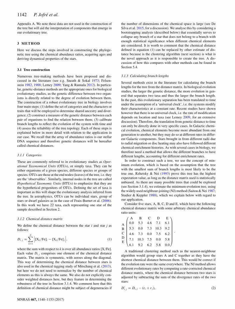
Consider five stars, A, B, C, D and E, which have the followingchemical distance matrix with some arbitrary chemical abundanceratio units:

ABCDE

⎛⎜⎜⎜⎜⎜⎜⎜⎜⎝

A B C D E0.0 5.3 4.6 7.1 6.1

5.3 0.0 7.3 10.3 9.2

4.6 7.3 0.0 7.5 6.2

7.1 10.3 7.5 0.0 5.8

6.1 9.2 6.2 5.8 0.0

⎞⎟⎟⎟⎟⎟⎟⎟⎟⎠

.

A traditional clustering method such as the nearest-neighbouralgorithm would group stars A and C together as they have theshortest chemical distance between them. This would be correct ifthe evolution rate were the same everywhere. The NJ method allowsdifferent evolutionary rates by computing a rate-corrected chemicaldistance matrix, where the chemical distance between two stars isadjusted by subtracting the sum of the divergence rates of the twostars:

D′i,j = Di,j − (ri + rj ), (2)

MNRAS 467, 1140–1153 (2017)

Phylogeny in the solar neighbourhood 1143

where Di, j are the elements of the chemical distance matrix definedin equation (1), n∗ is the number of stars and the divergence ratesare calculated as

rj =∑

i �=j Di,j

(n∗ − 2). (3)

The divergence rate is essentially the ‘mean’ chemical distance be-tween each of the two stars and the other stars. We note that thedenominator is n∗ − 2 rather than n∗ − 1 since we are consid-ering (n∗ − 1) stars for the star j. In our example, r2 would bethe divergence rate for star B, with a value (9.2 + 0.0 + 7.3 +10.3 + 5.3)/3 = 10.8.

A new node, ij, is defined for the two stars for which Dri,j is

minimal, i.e. the chemical distance between them is small comparedto how much those stars vary with every other star. The branchlengths from the new node ij to its ‘children’ i and j are calculatedas

Dij,i = Di,j + ri − rj

2, (4)

and similarly for Dij, j. The total branch length between i and j isstill just their chemical distance Di, j. Now a new distance matrixis constructed with the new node ij in place of i and j. This newdistance matrix contains (n∗ − 1) × (n∗ − 1) elements. The chemicaldistances to the new node are calculated as

Dij,k = Di,k + Dj,k − Di,j

2. (5)

If the element of the new matrix for which the rate-corrected chem-ical distance is smallest is between the new ij node and another star,say C, a new node is created that branches into the ij node and C.Otherwise the new node is created at the end of a new branch. Thewhole process is repeated until the tree topology is fully resolved.We only have dichotomies. The advantage of this method is thatit is very fast, which is crucial when dealing with a large sampleof taxa and when assessing the statistical significance of the tree(Section 3.1.4). Furthermore, this is a widely used method in biol-ogy, and therefore many implementations exist as packages. We usethe NJ method implemented in the software MEGA, v7.02 (Kumar,Stecher & Tamura 2016). This software, unlike many other codes,is able to construct trees from pre-defined distance matrices, ratherthan the original DNA sequences. Furthermore, MEGA can be easilycalled from PYTHON, which is important for studying the robustnessof the tree.

3.1.4 Assessing robustness

Inferring an evolutionary tree is an estimation procedure, in which a‘best estimate’ of the evolutionary history is made on the basis of in-complete information. In the context of molecular phylogenetics, amajor challenge is that many different trees can be produced from aset of observables. With 20 taxa, for example, there are close to 1022

trees of the type we have constructed (Dan & Li 2000). With currentspectroscopic surveys of Milky Way stars, we can have millions ofstars with detailed chemical abundances, producing an enormousnumber of tree possibilities. Here we use only 22 solar twins, butthis still implies a huge number of possible trees. Of course, manyof these have very low probability and therefore it is very importantto develop a statistical approach to infer the most probable treesamong this huge sample. Even if we use the NJ method to helpestimate the most likely tree, measurement errors in the abundance

2 http://www.megasoftware.net/home

ratios and systematic errors in our choice of elements to repre-sent the chemical sequence will distort the likelihood distribution.It is therefore crucial before interpreting the tree and reconstruct-ing the evolutionary history of our sample of stars to ensure thatour final tree is robust by means of statistical techniques (see e.g.Felsenstein 1988, for a discussion).

Here, our robust tree was obtained by combining a Monte Carlomethod that explores measurement error with a bootstrapping proce-dure that explores alternative definitions of the chemical sequence.

(i) Monte Carlo simulations. This is a widely used method forpropagating uncertainties in measured quantities. The measurementerrors in the abundance ratios are of the order of 0.01 dex. Usingthose listed in table 4 of Nissen (2015) and table 2 of Nissen (2016),we generate new data matrices by drawing from Gaussian distribu-tions with means equal to the abundance ratios in the old data matrixand dispersions equal to the measured errors. In doing this, we as-sume the errors in [Fe/H] are very small and therefore essentiallyindependent.

(ii) Bootstrapping/jackknifing. This is commonly employed inevolutionary studies, where random characters in the DNA sequenceare removed from the data matrix. As our chemical sequences aresignificantly shorter than DNA sequences – 17 abundance ratiosin comparison to millions of genes – we instead create alternativechemical sequences in which the length of the chemical sequenceis kept constant at 17 using the new data matrix generated by theMonte Carlo method. These are created by generating a randomsequence of the original 17 abundance ratios, using sampling withreplacement. Thus we obtain chemical sequences that may not con-tain all the elements, and the elements that are included will have arandom weight.

1000 resamples of the original data matrix are produced using thecombined Monte Carlo and bootstrapping method, each consistingof 22 stars and a chemical sequence of length 17. New chemicaldistance matrices and trees are calculated for each resample. Aconsensus tree is then built from the 1000 trees using the softwareMESQUITE, v3.10.3 A majority-rule consensus method is used forwhich branches only appear that are statistically significant, i.e. thatappear in a non-conflictive way in at least 50 per cent of the trees.The majority-rule consensus method is particularly important forassessing the significance of very short branches. If these branchesare not statistically significant, they are removed and polytomies(more than two branches extending from one node) are obtainedrather than dichotomies (two branches extending from one node).This is important because a fundamental concept in evolutionary bi-ology studies is that natural processes divide a population into two,enabling further independent evolution in dichotomies. Polytomies,on the other hand, are interpreted as a burst of diversification: manyspecies diverging at the same time, with a single origin. In biol-ogy this is rather unlikely, and therefore polytomies are treatedwith caution and interpreted as unresolved data or incomplete data(Felsenstein 1988). In Galactic chemical evolution however, poly-tomies are expected consequences of star formation bursts and there-fore constructing the majority-rule consensus tree is a fundamentalstep of applying phylogenetics in our case.

We comment that Monte Carlo simulations are standard methodsto assess the robustness of trees in evolutionary biology. Theseare combined with bootstrapping by adding and removing genes(chemical elements in our case). There might be other approaches to

3 http://mesquiteproject.org/

MNRAS 467, 1140–1153 (2017)

1144 P. Jofre et al.

do this, but they do not seem in biology to be competitive enough toreplace the standard Monte Carlo and bootstrapping methods. Somemore sophisticated methods have been proposed in the literature,like the double bootstrap (e.g. see Ren, Ishida & Akiyama 2013,for recent discussion). These methods however do not significantlyimprove results with respect to standard methods but lower downthe computational time to obtain final trees, which is relevant whenlarge data sets are being analysed. A discussion of this can be alsofound in Ropiquet, Li & Hassanin (2009).

It is true that in astrophysics this could be different, but here weare trying to make the first step, which is to use what are the standardtechniques in biology. Since we do not find anything conflictive inour results (below), we believe that applying this is sufficient forthis first step. Certainly when numerical simulations and largerdata sets are used, more sophisticated techniques will have to beexplored.

3.2 Ages and dynamical properties

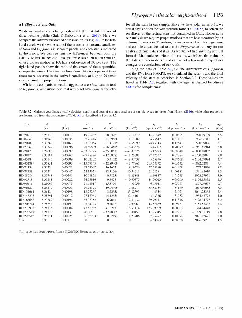
Knowledge of stellar ages will help explore how chemical distancescorrelate with time in identified stellar populations, and in the casesthey do, quantify how the rates differ between them. The ages used inthis work (Table A2) are taken from Nissen (2015, 2016), which arederived considering the stellar parameters and isochrones. Combin-ing ages with dynamical properties will help interpret the differentbranches that appear in the consensus tree. We calculate dynami-cal properties, using the astrometric and kinematic information inTable A1. To convert from heliocentric coordinates to Galactocen-tric coordinates, we assume that the Sun is located at (R0, z0) = (8.3,0.014) kpc (Schonrich 2012), that the local standard of rest (LSR)has an azimuthal velocity of 238 km s−1, and that the velocity of theSun relative to the LSR is (vR, vφ , vz) = (−14.0, 12.24, 7.25) km s−1

(Schonrich 2012).We calculate the velocities (U, V, W) of the stars in heliocen-

tric Cartesian coordinates, which tell us the velocities of the starswith respect to the Sun. We also calculate the actions Jr, Jφ andJz of the stars, which quantify the extent of the star’s orbit inthe radial, azimuthal and vertical directions. In an axisymmetricsystem, Jφ is simply the z component of the angular momentumLz. The actions will help identify which Galactic component thestars belong to as we would expect thin-disc stars to be on nearcircular orbits in the equatorial plane and therefore have a smallJr and Jz. The actions can be calculated from Cartesian coordi-nates using the Stackel Fudge, given some gravitational potentialassumed for the Galaxy. We use the composite potential proposedby Dehnen & Binney (1998), generated by thin and thick stellardiscs, a gas disc and two spheroids representing the bulge and thedark halo. We use the potential parameters of Piffl et al. (2014)and the implementation of the Stackel Fudge by Vasiliev et al.(in preparation), which is part of the Action-based Galaxy Mod-elling Architecture (AGAMA).4 In calculating the velocities and ac-tions of the stars, we propagate the errors in the astrometric andkinematic data, using 1000 Monte Carlo samples to estimate themean and dispersion. The dynamical properties can be found inTable A2.

4 AGAMA can be downloaded from https://github.com/GalacticDynamics-Oxford/AGAMA

4 R ESULTS

4.1 The consensus tree

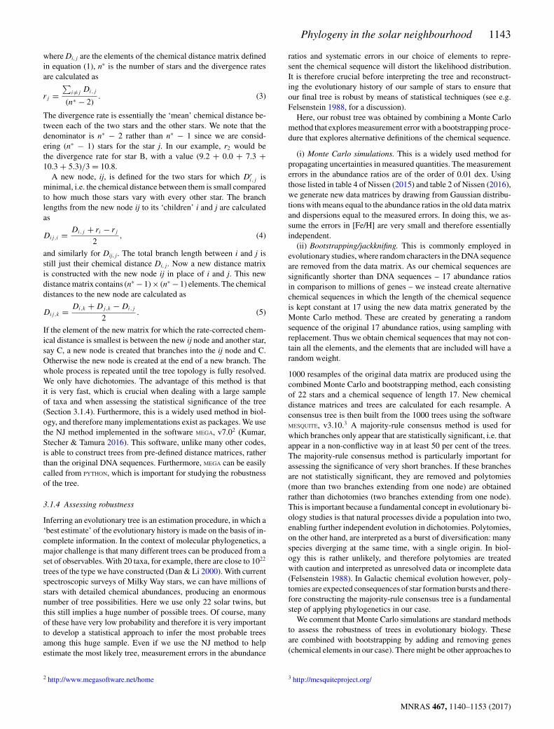
Fig. 1 presents our consensus tree. A tree constructed with the NJmethod is ‘unrooted’, and therefore even if clusters of stars appearto branch off initially from the same point, it does not signify thisis the beginning of the evolution of system. The radiation format(Fig. 1) for a phylogenetic tree is particularly suitable for visual-izing such trees as it emphasizes that the groups and unclassifiedstars are separate from each other. The length of the branches is inchemical dex units with the scale indicated in the legend. They rep-resent the chemical distance between each star and the node fromwhich it emerged. The chemical distance between any two starsis determined by adding up the lengths of the branches betweenthem.

The NJ method alone would only produce dichotomies, i.e. nodessplit into two branches. However, the application of the majority-rule consensus method results in several polytomies, showing thatsome of the branches found in each of the 1000 trees in the resam-pling were not significant. Such polytomies could be expected inchemical evolution when star formation bursts can result in severalstars driving different chemical enrichment paths, not just two.

Even with the polytomies, three main stellar populations, i.e.groups of stars sharing a common ancestor, are identified. The firstone (red) includes the following stars: the Sun, HD 2071, HD 45184,HD 146233, HD 8406, HD 92719, HD 27063, HD 96116 andHD 134664. A second stellar population (blue) includes the stars:HD 210918, HD 45289 and HD 220507. A third stellar population(orange) appears to be equally independent from the other two pop-ulations and includes the stars HD 78429, HD 208704, HD 20782and HD 38277. Finally, six stars (black) cannot be assigned toany population with enough statistical confidence. These stars areHD 28471, HD 96423, HD 71334, HD 222582, HD 88084 andHD 183658. We comment here that perhaps a different definition ofchemical distance than the one employed in equation (1) might helpto allocate some of these six stars into one of the populations withbetter confidence but this is beyond the purpose of this work. Herewe want to show that it is possible to apply phylogenetic analysesand tree thinking in the field of Galactic archaeology. In this workwe call these stars simply ‘undetermined’.

The branch lengths of the red stellar population are short, of theorder of 0.1 dex, except for HD 96116, which has a branch length ofalmost 0.4 dex. The branch lengths of the orange stellar populationare also of the order of 0.1 dex, reflecting that these stars are verychemically similar to each other. The branch lengths between theoriginal polytomy and the first node in the blue stellar populationare significantly larger than the first nodes in the red and orangepopulations, but the branch lengths between nodes are of the sameorder of magnitude, with the exception of HD 220507, which has abranch length of 0.3 dex.

For guidance, the ages of the stars are indicated next to theirnames in Fig. 1. The star furthest along the red right branch,HD 96116, is the youngest star of the sample (0.7 Gyr). It is moreseparate from the other stars in the red stellar population due toa larger chemical distance, and this is reflected in the ages of theother stars, which are clustered between 2.4 and 4.5 Gyr. The orangestellar population has stars that are chemically very similar to eachother. Their ages are also in a restricted range of 0.9 Gyr between7.4 and 8.3 Gyr.

The star furthest along the blue branch, HD 220507, is also theoldest star of the sample (9.8 Gyr). The other two stars in this

MNRAS 467, 1140–1153 (2017)

Phylogeny in the solar neighbourhood 1145

Figure 1. Unrooted phylogenetic tree. Three main branches are obtained and coloured with blue, red and orange. Stars that do not belong to any branch withstatistical significance are coloured with black. Branch lengths are in dex units, with the scale indicated at the bottom of the diagram.

branch have ages of 9.1 and 9.4 Gyr. The chemical distance betweenthe youngest star and the oldest star is the largest in the tree at1.6 dex and is obtained by adding the length of all the branches thatseparate the stars. The undetermined stars have ages between 5.2 and8.8 Gyr.

The mean age of all stars in a given population is indicated at thebottom of Fig. 1, following the colour coding of the branches. Wecan see that the stellar populations have different ages, with timeincreasing from left to right. The ages have told us that there isa very old stellar population (blue branch), a slightly younger butstill old population (orange branch), stars of intermediate age (blackbranches) and a young stellar population (red branch). We remarkhere that age was not used to build the tree.

Thus, the tree of Fig. 1 adds a rough direction to the evolutionaryprocesses, i.e. the older stars are found towards the left, while theyounger stars are found towards the right. However, it is clear that inthe region of overlap between the red, black and blue branches, thestars belonging to separate stellar populations may have been pro-duced from gas that was chemically enriched at different rates andexposed to dynamical processes such as heating and radial migra-tion. Therefore their location in this region is no longer indicativeof their age. We will come back to the importance of dynamicalprocesses in Section 5.

4.2 Dynamics of the identified stellar populations

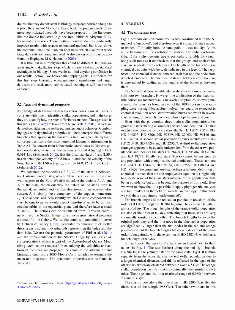
In order to study the nature of the identified stellar populationsmore clearly, we look at dynamical properties of the stars. Theleft-hand panel of Fig. 2 shows the classical Toomre diagram. They-axis indicates the contribution to the star’s velocity in directionsperpendicular to that of Galactic rotation and the x-axis indicates thecontribution to the star’s velocity along Galactic rotation, compared

to that of the Sun. Thin-disc stars should behave like the Sun,while thick disc and halo stars have velocities in random directions.Therefore the stars in the red population that cluster around zero inboth directions, and include the Sun, behave like thin-disc stars. Theother populations and undetermined stars cover a larger range in thisplot, but in general tend to have higher values in both directions andare therefore more likely to be thick-disc stars. They are unlikely tobe halo stars because they are comparatively metal rich.

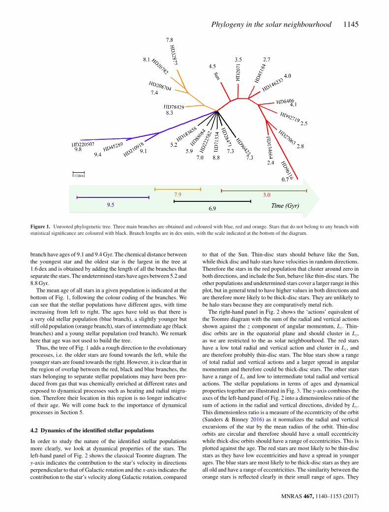
The right-hand panel in Fig. 2 shows the ‘actions’ equivalent ofthe Toomre diagram with the sum of the radial and vertical actionsshown against the z component of angular momentum, Lz. Thin-disc orbits are in the equatorial plane and should cluster in Lz,as we are restricted to the as solar neighbourhood. The red starshave a low total radial and vertical action and cluster in Lz, andare therefore probably thin-disc stars. The blue stars show a rangeof total radial and vertical actions and a larger spread in angularmomentum and therefore could be thick-disc stars. The other starshave a range of Lz and low to intermediate total radial and verticalactions. The stellar populations in terms of ages and dynamicalproperties together are illustrated in Fig. 3. The y-axis combines theaxes of the left-hand panel of Fig. 2 into a dimensionless ratio of thesum of actions in the radial and vertical directions, divided by Lz.This dimensionless ratio is a measure of the eccentricity of the orbit(Sanders & Binney 2016) as it normalizes the radial and verticalexcursions of the star by the mean radius of the orbit. Thin-discorbits are circular and therefore should have a small eccentricitywhile thick-disc orbits should have a range of eccentricities. This isplotted against the age. The red stars are most likely to be thin-discstars as they have low eccentricities and have a spread in youngerages. The blue stars are most likely to be thick-disc stars as they areall old and have a range of eccentricities. The similarity between theorange stars is reflected clearly in their small range of ages. They

MNRAS 467, 1140–1153 (2017)

1146 P. Jofre et al.

Figure 2. Toomre diagram (left) and the sum of the radial and vertical actions shown against the z component of angular momentum (right). Stellar populationsare coloured according to the classification of the tree of Fig. 1.

Figure 3. Eccentricity against age of the stars for the stellar populationsand undetermined stars identified in Fig. 1.

have a range in eccentricities that is intermediate between the thinand thick discs.

The undetermined stars randomly span the ages between the thinand thick discs with a range of eccentricities intermediate betweenthe thin-disc and thick-disc stars. Some of these stars could belongto the older, flared part of the thin disc and the oldest may belong tothe thick disc. The small number of data points means however thatif this were the case, the connection between these stars and thosein the thin and thick discs could not be recovered.

It should also be noted that the trend followed by thestars is continuous, restating the age–velocity dispersion relation(Wielen 1977), i.e. older stars have a higher velocity dispersion andtherefore lie on more eccentric orbits. There is no evidence fromthis plot that the data require separate components, and thereforea more careful inspection of the abundance ratios is required (seeSection 5).

4.3 Evolution of stellar populations

To go further than simply identifying stellar populations, the phy-logenetic nature of the tree allows us to investigate the evolution ofchemical abundances within each stellar population. For example,any time a branch splits (i.e. there is a dichotomy or polytomy),we can interpret this as an instance at which the evolution of thegas diverged. The stars arising from the split have formed from thesame or similar gas clouds. The further away a star in the poly-

tomy is from the node the more evolved a gas cloud from which itoriginated.

We study the chemical evolution within these different Galacticcomponents by exploiting the phylogenetic nature of the tree. Todo so, we redraw the tree of Fig. 1, using a classical format inFig. 4, as this allows us to inspect the individual branch lengths inmore detail. The Galactic components assigned to each branch areindicated on the left and stellar ages on the right for guidance. Sincewe focus here only on stars that are assigned to a branch with enoughstatistical relevance, we consider the blue, red and orange branchesindependently, and calculate the total branch length starting fromthe vertical line. This is done by adding up the values indicated ineach branch from the vertical line to each star. In Fig. 5 we show thebranch length and age (BLA) relation, finding that branch lengthdecreases with stellar age for the thick-disc (blue stars) but increaseswith stellar age for the thin-disc and intermediate stars (red andorange stars). This is simply a consequence of the location of thezero-point in the tree. We would expect environmental processes anddynamical processes that have brought stars from a very differentpart of the Galaxy to branch out as separate stellar populations.Therefore within each branch we would expect a monotonic trendof stars increasing their elemental abundances with time. However,stars brought in from radii near to the solar neighbourhood may beallocated to the same branch, adding scatter to this trend. We cantherefore make an estimate of the mean chemical evolution rate andcontributions from dynamical processes by carrying out linear fits(dashed lines in Fig. 5). Below we discuss the chemical evolutionhistory for the different groups of stars.

Thin disc. The BLA relation for the thin-disc stars is shown in redin Fig. 5. The stars are not consistent with being a single age, andtherefore the stars are likely to have formed in successive multiplebursts of star formation rather than a single burst. As suggested bythe tree, the stellar age generally correlates approximately linearlywith total branch length. Therefore we can make an estimate ofthe mean chemical evolution rate, 〈�XFe〉, by adding up all thebranch lengths between the node from which the Sun emergedand HD 96116 to obtain a total chemical distance of 0.673 dex.This distance emerged within a period of 4 Gyr, and therefore anindication of the mean chemical evolution rate can be obtained bydividing the total chemical distance by the difference in ages to get〈�XFe〉 = 0.168 dex Gyr−1.

We also notice in Fig. 5 that there is a significant degree ofscatter about the straight-line fit of the BLA relation (i.e. assuming

MNRAS 467, 1140–1153 (2017)

Phylogeny in the solar neighbourhood 1147

Figure 4. Phylogenetic tree of 22 solar twins in the solar neighbourhood, created using 17 elemental abundances. Stellar populations are assigned consideringthe age and the dynamical properties of the stars and are indicated at the right. Branch lengths have units in dex, with the scale indicated at the left bottom.

Figure 5. Stellar age against branch length measured from the verticaledge from which the thin-disc branch (red), thick-disc branch (blue) andintermediate population branch (orange) emerge.

that the mean chemical evolution rate is constant with time), whichmean coeval stars show a different level of chemical evolution. Starsdeviating more than 1σ from the fit are enclosed with a circle, andtheir name indicated. These stars may be good candidates to havearrived to the solar neighbourhood via radial migration because

their eccentricities do not stand out from the rest of the thin-discstars.

Thick disc. The stellar ages against total branch length for the thick-disc stars are plotted in blue in Fig. 5. The stars in this case areconsistent with being a single age, and therefore could have formedfrom a single burst, but the diversification in chemical sequencessuggests they were not all formed at exactly the same time. There-fore the burst was not instantaneous. As with the thin-disc stars,the BLA relation is linear, although we must emphasize that in thiscase the data are also consistent with a zero-gradient curve. Makinga simple estimate of the chemical evolution rate as with the thindisc, we obtain a total chemical distance of 0.473 dex and a totalage span of 0.7 Gyr. This gives a rate of 〈�XFe〉 = 0.657 dex Gyr−1,i.e. a higher rate compared to the thin disc.

Intermediate. The orange stars of Fig. 5 lack a clear evolution di-rection, i.e. the BLA relation is not evident. The stellar ages canalso be seen to be relatively consistent with each other within theerrors. Therefore, like the thick disc, these stars could have formedin a single burst and again the small level of diversification inchemical sequences suggests that the burst was not instantaneous.Despite the lack of a clear direction of chemical evolution, we canstill place a lower limit on the chemical evolution rate by con-sidering that a total branch length of 0.269 dex was experiencedwithin 1 Gyr, giving a lower limit on the chemical evolution rate of〈�XFe〉0.269 dex Gyr−1, which is in between both populations.

Undetermined. The black stars do not form a branch themselvesin Fig. 4, and therefore we cannot include them in Fig. 5.

MNRAS 467, 1140–1153 (2017)

1148 P. Jofre et al.

A B C D E

F G H I J

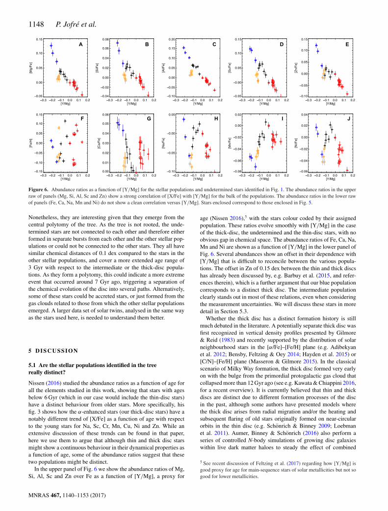
Figure 6. Abundance ratios as a function of [Y/Mg] for the stellar populations and undetermined stars identified in Fig. 1. The abundance ratios in the upperraw of panels (Mg, Si, Al, Sc and Zn) show a strong correlation of [X/Fe] with [Y/Mg] for the bulk of the populations. The abundance ratios in the lower rawof panels (Fe, Ca, Na, Mn and Ni) do not show a clean correlation versus [Y/Mg]. Stars enclosed correspond to those enclosed in Fig. 5.

Nonetheless, they are interesting given that they emerge from thecentral polytomy of the tree. As the tree is not rooted, the unde-termined stars are not connected to each other and therefore eitherformed in separate bursts from each other and the other stellar pop-ulations or could not be connected to the other stars. They all havesimilar chemical distances of 0.1 dex compared to the stars in theother stellar populations, and cover a more extended age range of3 Gyr with respect to the intermediate or the thick-disc popula-tions. As they form a polytomy, this could indicate a more extremeevent that occurred around 7 Gyr ago, triggering a separation ofthe chemical evolution of the disc into several paths. Alternatively,some of these stars could be accreted stars, or just formed from thegas clouds related to those from which the other stellar populationsemerged. A larger data set of solar twins, analysed in the same wayas the stars used here, is needed to understand them better.

5 D ISCUSSION

5.1 Are the stellar populations identified in the treereally distinct?

Nissen (2016) studied the abundance ratios as a function of age forall the elements studied in this work, showing that stars with agesbelow 6 Gyr (which in our case would include the thin-disc stars)have a distinct behaviour from older stars. More specifically, hisfig. 3 shows how the α-enhanced stars (our thick-disc stars) have anotably different trend of [X/Fe] as a function of age with respectto the young stars for Na, Sc, Cr, Mn, Cu, Ni and Zn. While anextensive discussion of these trends can be found in that paper,here we use them to argue that although thin and thick disc starsmight show a continuous behaviour in their dynamical properties asa function of age, some of the abundance ratios suggest that thesetwo populations might be distinct.

In the upper panel of Fig. 6 we show the abundance ratios of Mg,Si, Al, Sc and Zn over Fe as a function of [Y/Mg], a proxy for

age (Nissen 2016),5 with the stars colour coded by their assignedpopulation. These ratios evolve smoothly with [Y/Mg] in the caseof the thick-disc, the undetermined and the thin-disc stars, with noobvious gap in chemical space. The abundance ratios of Fe, Ca, Na,Mn and Ni are shown as a function of [Y/Mg] in the lower panel ofFig. 6. Several abundances show an offset in their dependence with[Y/Mg] that is difficult to reconcile between the various popula-tions. The offset in Zn of 0.15 dex between the thin and thick discshas already been discussed by, e.g. Barbuy et al. (2015, and refer-ences therein), which is a further argument that our blue populationcorresponds to a distinct thick disc. The intermediate populationclearly stands out in most of these relations, even when consideringthe measurement uncertainties. We will discuss these stars in moredetail in Section 5.3.

Whether the thick disc has a distinct formation history is stillmuch debated in the literature. A potentially separate thick disc wasfirst recognized in vertical density profiles presented by Gilmore& Reid (1983) and recently supported by the distribution of solarneighbourhood stars in the [α/Fe]–[Fe/H] plane (e.g. Adibekyanet al. 2012; Bensby, Feltzing & Oey 2014; Hayden et al. 2015) or[C/N]–[Fe/H] plane (Masseron & Gilmore 2015). In the classicalscenario of Milky Way formation, the thick disc formed very earlyon with the bulge from the primordial protogalactic gas cloud thatcollapsed more than 12 Gyr ago (see e.g. Kawata & Chiappini 2016,for a recent overview). It is currently believed that thin and thickdiscs are distinct due to different formation processes of the discin the past, although some authors have presented models wherethe thick disc arises from radial migration and/or the heating andsubsequent flaring of old stars originally formed on near-circularorbits in the thin disc (e.g. Schonrich & Binney 2009; Loebmanet al. 2011). Aumer, Binney & Schonrich (2016) also perform aseries of controlled N-body simulations of growing disc galaxieswithin live dark matter haloes to steady the effect of combined

5 See recent discussion of Feltzing et al. (2017) regarding how [Y/Mg] isgood proxy for age for main-sequence stars of solar metallicities but not sogood for lower metallicities.

MNRAS 467, 1140–1153 (2017)

Phylogeny in the solar neighbourhood 1149

spiral and giant molecular cloud heating on the discs. In these mod-els the outward-migrating populations are not hot enough verticallyto create thick discs. Other chemodynamical models and cosmolog-ical simulations (Chiappini, Matteucci & Gratton 1997; Kobayashi& Nakasato 2011; Minchev, Chiappini & Martig 2013; Minchevet al. 2015) consider further infall of gas via, e.g. mergers thatagree with many observables, such as the height of the disc and themetallicity and abundance gradients as a function of radius. Unfor-tunately, the mechanisms of mergers for instance are still poorlyunderstood.

Our results support a separation between thin and thick disc pop-ulations represented by two independent branches of stars evolvingat different rates, suggesting that these populations have differentformation histories.

5.2 The contribution of dynamical processes

Dynamical processes such as disc heating and radial migration bringin stars to the solar neighbourhood that have different birth radii.Therefore metal-richer stars born in the inner Galaxy and metal-poorer stars born in the outer Galaxy can be brought into the so-lar neighbourhood. The relation between branch length and stellarage in Fig. 5 for our small sample of stars however suggests thatchemical enrichment is the primary driver for changes in chemicaldistances in the stellar populations, even in the component iden-tified as the thin disc, where dynamical processes are thought tobe more prevalent. This may be because disc-heated and radiallymigrated stars that came from very different parts of the Galaxyend up in a different stellar population (e.g. the intermediate stars)or not allocated to any stellar population (the undetermined stars).However there is also a scatter in the branch length–stellar age re-lation for thin-disc stars, which could arise from disc-heated andradially migrated stars whose birth origin is not too far from thesolar neighbourhood. They could have been formed from similarlychemically enriched gas at the same stellar age.

Fig. 6 shows that the contribution to the scatter in the BLA relation(Fig. 5) for the thin-disc stars arises primarily from scatter in the[Fe/H], and to some extent scatter in other elements of the lowerpanel of that figure. This suggests that some elements are morevulnerable to radial gas flows than others, and therefore are goodtracers of dynamical processes. On the other hand, the elements ofthe upper panels of Fig. 6 have a well-defined trend, suggesting thatthey are good tracers for studying chemical enrichment history.

5.3 What is the origin of the intermediate population?

The intermediate population is significantly distinct in the chemicalplots of Fig. 6 except in the case of Fe, for which three of them areslightly metal poor and the fourth is metal richer. They cluster inother elemental abundances and age, but have lower levels of the α

elements (Mg, Si, Ca, S and O) and Al, Na, Cu, Sc and Zn than starsfrom the thin or thick discs with the same [Y/Mg]. The stars have aspread in actions and lie on the same trend in age and eccentricity asthe other stars in the sample, i.e. they are part of the same dynamicalsystem as the other stars. Stars with intermediate α abundances havealready been noted in the past (Edvardsson et al. 1993) and recentlydiscussions of their nature have become more active. They might berelated to the high-α metal-rich stars discussed in Adibekyan et al.(2012) as they were shown to be older and more α-enhanced than thetypical thin-disc stars. Intermediate-α stars have also been recentlydiscussed in Allende Prieto, Kawata & Cropper (2016), who foundthem to display intermediate dynamical behaviour between thin and

Figure 7. Sodium- versus nickel-to-iron abundance ratios for the stars olderand kinematically hotter than the thin-disc population.

thick discs, as in this study. Whether such stars are part of the thinor thick disc is still not known.

The intermediate stars could have been born at a different radiusin the Milky Way, and brought into the solar neighbourhood by ra-dial migration or disc heating. However we would not expect suchstars to cluster so strongly in abundance and age. Their chemistrysuggests that they were born from a gas cloud that suffered froma different chemical enrichment history than the rest of the starsin our sample. An accretion of a smaller system in the past is apossibility. The shallower gravitational potential in smaller systemsis less efficient at retaining the gas of stellar explosions that occurwhen massive stars die. Therefore elements such as Na, Ni, Cu,Zn and α-elements, which are mostly produced in massive stars(see Nomoto, Kobayashi & Tominaga 2013, for a review of theproduction sites of these elements), tend to be lower in these sys-tems (Tolstoy, Hill & Tosi 2009; Nissen & Schuster 2010; Bensbyet al. 2014). Furthermore, as extensively discussed in these papers,in the [Na/Fe]–[Ni/Fe] diagram, accreted stars appear systemati-cally at the lower end. In Fig. 7 we show these abundance ratiosfor our sample of stars. Here, following e.g. Bensby et al. (2014),we omit the thin-disc (red) stars as they correspond to the kinemat-ically cold population. We can see that the intermediate populationhas lower [Na/Fe] and [Ni/Fe] abundance ratios than the thick discstars, consistent with these stars being accreted.

Dwarf galaxies as potential progenitors for these stars are proba-bly ruled out as those in the Local Group tend to have much lowermetallicities than solar. Only Sagittarius achieves solar metallicity(e.g. Tolstoy et al. 2009). If a merger is responsible, it must have oc-curred around the time the stars were born, as the age–eccentricityplot shows that they have become part of the Milky Way dynamicalsystem. Furthermore, since the stars have solar metallicities, theprogenitor must have been significantly more massive than typicaldwarf galaxies.

Studies focused on the density profiles of metal-poor halo stars,such as that one of Deason et al. (2013), suggest that the Milky Waybroken profile can be associated with an early and massive accretionevent. Several works have found signatures of past accretion eventsin the Milky Way by assessing clustering in age and abundancespace (e.g. Helmi et al. 2006; Bensby et al. 2014). However, Ruchtiet al. (2015) searched for evidence of an accreted disc componentin a sample of almost 5000 stars in the Gaia-ESO spectroscopicsurvey with no success. This may be because they initially searchedin phase space, in which these stars may already be dispersed, andthey only used [Mg/Fe] abundance ratios to search for chemicallydistinct stars, or because there is simply none of such stars in thesolar neighbourhood. Since evidence of an early accreted material of

MNRAS 467, 1140–1153 (2017)

1150 P. Jofre et al.

solar-metallicity stars in the solar neighbourhood has not been found(see Ruchti et al. 2015, and references therein), it seems difficult toensure that the intermediate population corresponds indeed to suchstars given the relatively large number of them we find in our smallsample. A more detailed dynamical analysis of these interestingstars would be required to understand their origin.

5.4 How does a phylogenetic approach compareto other methods?

The use of chemical patterns of stars as a method for identifyingseparate populations that have been either born at different radii, dif-ferent Galactic components, or even extragalactic systems, alreadyforms the basis of chemical tagging studies (Freeman & Bland-Hawthorn 2002; Bland-Hawthorn, Krumholz & Freeman 2010).In its simplest form, populations of solar neighbourhood stars areseparated in the [α/Fe]–[Fe/H] diagram (Mikolaitis et al. 2014;Hawkins et al. 2015) or Toomre diagram (Bensby, Feltzing &Lundstrom 2003; Hattori & Gilmore 2015) to identify differentpopulations, in particular the thin and thick discs. Slicing popu-lations, according to some criterion, as in the earlier studies caninduce biases. They can be of a kinematic or chemical nature.For example, it is not fully established yet that the thick disc de-fined as the ‘high-α/Fe’ disc is the same as the kinematically hotdisc or the old disc selected from [C/N] abundances (Masseron &Gilmore 2015) for example. This leads to the problem that slic-ing populations like this makes it very difficult to study the inter-face between the thin-disc and thick-disc populations, especially atsolar metallicities (see discussion in, e.g. Adibekyan et al. 2012;Wojno et al. 2016) where the α/Fe ratios of both populations arevery similar.

Furthermore, there is still no consensus to what is the best def-inition of the ‘high-α/Fe’ stars. One reason is that in the [α/Fe]–[Fe/H] diagram, there is an ‘intermediate-α’ population lying be-tween the thin- and thick-disc populations (Edvardsson et al. 1993),probably related to our orange population. This population is eithersplit between the thin and thick discs (Kordopatis et al. 2015) orsimply rejected from the analyses (Hawkins et al. 2015; Masseron& Gilmore 2015). This becomes especially uncertain at solar metal-licities, where the [α/Fe] of the two populations overlaps (see dis-cussions in, e.g. Nidever et al. 2014).

Last but not least, survey selection function plays a crucial role inthis matter. For example, it is not clear what happens to the high α/Fedisc as we approach the Galactic Centre. It may not be the same asthe high velocity dispersion disc of the solar neighbourhood. Cutsto define populations might be useful locally only. Survey selectionfunction also affects the topology of trees, without a well-definedselection function of our data set we cannot give a global picture ofhow the evolution of the populations found as branches in the localtree takes place.

With the advent of new surveys, millions of high-resolution spec-tra are now available for a number of elements that can be used inthe hope to define a unique chemical sequence. A particular chal-lenge with an increasing number of chemical abundances is howbest to combine them for identifying separate populations. Tinget al. (2012) and Blanco-Cuaresma et al. (2015) apply a princi-pal component analysis (PCA), which transforms a set of variablesthat are possibly correlated into a smaller set of linearly uncorre-lated variables called principal components. Mitschang et al. (2013)combine weighted absolute distances in a large number of chemicalelements between two stars into a single metric and use this as thebasis for deriving a function that describes the probability that two

stars of common evolutionary origin. Hogg et al. (2016) identifyoverdensities in a 15-dimensional chemical-abundance space pro-vided by Apache Point Observatory Galactic Evolution Experiment(APOGEE) data, using the k-means algorithm, which is a methodfor clustering points in a high-dimensional space. This algorithmhas also been applied as a basis in the chemical tagging work ofBland-Hawthorn et al. (2010) but with less chemical elements andlater on confirmed with simulations in Feng & Krumholz (2014).While PCA assumes that the variables are linearly correlated, thenumber of stellar populations needs to be defined a priori for thek-means clustering algorithm.

A phylogenetic method offers a multivariate approach that doesnot assume linearity, does not need the number of stellar popula-tions to be specified beforehand and does not need to artificiallyslice populations. The implementation presented here with the NJmethod improves on traditional clustering metrics, by normaliz-ing the chemical distance by the degree to which the stars varyfrom all other stars. Phylogeny also offers a very simple visual-ization of separate stellar populations that additionally orders thestars within them according to chemical distance. This can then beused to compare chemical enrichment rates between stellar pop-ulations and obtain an insight into the importance of dynamicalprocesses in shaping the distribution of chemical elements in sam-ples of stars. Trees allow us to test hypotheses about both historyand process and therefore their analysis goes much beyond be-ing an efficient clustering algorithm like other chemical taggingtechniques.

5.5 Uncertainties in the analysis

Perhaps the largest uncertainty in our analysis is the small samplesize. The resulting consequence is that some connections betweenstars may have been missed, thus not allowing a full recovery of thechemical enrichment history.

In addition, we have only explored a single method for con-structing the phylogenetic tree (NJ, see Section 3). Although wehave assessed the robustness of applying this particular method,there are several other methods in the literature that may result indifferent groupings and branch lengths, and therefore a differentphylogeny. There are other ways of constructing the distance ma-trix and translating this into a tree. There are also methods thatdo not rely on constructing a distance matrix. Particular types ofevolutionary events can be penalized in the construction of the treecost, and then an attempt is made to locate the tree with the small-est total cost. The maximum likelihood and Bayesian approachesassign probabilities to particular possible phylogenetic trees. Themethod is broadly similar to the maximum-parsimony method butallows both varying rates of evolution and different probabilities ofparticular events. While this method is computationally expensiveand therefore not easy to use for large data sets, it remains to betested in future applications within Galactic archaeology.

As with chemical tagging studies, the method presented hererelies on the uniqueness of stellar DNA. We ascertain that as longas enough elements are used in the analysis, this should be the case(Hogg et al. 2016). We need to be aware however that our sampleneeds to be chosen such that the chemical distances are reflectingdifferences in chemical evolution and not systematic differences dueto internal processes happening in stars, such as atomic diffusion(e.g. Gruyters et al. 2013), pollution due to binary companions(McClure, Fletcher & Nemec 1980) or even enrichment due toaccretion of gas from the ISM (Shen et al. 2016). Therefore it isimportant to have a sample of stars with the same spectral class

MNRAS 467, 1140–1153 (2017)

Phylogeny in the solar neighbourhood 1151

(see e.g. extensive discussion in Blanco-Cuaresma et al. 2015; Jofreet al. 2015a, 2016).

6 SU M M A RY A N D C O N C L U S I O N S

We demonstrate the potential for the use of a phylogenetic methodin visualizing and analysing the chemical evolution of solar neigh-bourhood stars, using abundances of 17 chemical elements for the22 solar twins of Nissen (2015, 2016) as a proxy for DNA. Thechemical abundances were used to create a matrix of the chemicaldistances between pair of stars. This matrix was input into a soft-ware developed for molecular biology to create a phylogenetic tree.Despite the small size of the sample, we believe that the methodsuccessfully recovered stellar populations with distinct chemicalenrichment histories and produced a succinct visualization of thestars in a multidimensional chemical space.

A comparison of the order of the stars along tree branches withstellar ages confirmed that the order generally traces the directionof chemical enrichment, thus allowing an estimate of the meanchemical enrichment rate to be made. Chemical enrichment has amean rate of 〈�XFe〉 = 0.168 dex Gyr−1 in the thin disc, 〈�XFe〉 =0.657 dex Gyr−1 in the thick disc and 〈�XFe〉 = 0.269 dex Gyr−1 inthe intermediate population of stars. Our analysis thus confirms, ina purely empirical way, that the star formation rate in the thick discis much faster than that in the thin disc.

In addition to confirming a likely separate chemical enrichmenthistory in the thin disc compared to the thick disc, we also finda separate population, intermediate in age and eccentricities butdistinct and clustered in several abundance ratios. Because of itsold age and low abundances of α- and other iron-peak elementswith respect to coeval stars in the thin- and thick-disc populations,we surmise that these stars could have arrived via a major merger atthe early stages of the Milky Way formation. We however could notrule out the possibility that these stars might be the youngest tail ofthe thick disc or the oldest tail of the thin disc, as they belonged tosimilar trends in some abundance ratios and kinematical properties.The fact they emerge as an independent branch in our tree could beeither due to a truly different nature or due to selection effects. Weconclude that a more detailed dynamical study of such stars and alarger sample of old solar-metallicity stars is necessary. Future workwill also benefit greatly from tests on simulated stars in the solarneighbourhood in order to better understand how radially migratedand disc heated stars appear in the phylogenetic tree.

In biology it is commonly said that to study evolution, one essen-tially analyses trees. Galactic archaeology should be no different,especially now, during its golden ages. Thanks to Gaia and its com-plementary spectroscopic and asteroseismic surveys, we are quicklygetting chemical abundances of millions of stars that can be com-plemented with accurate astrometry and ages. These rich data setsare on the verge of putting us closer to finding the one tree thatconnects all stars in the Milky Way.

AC K N OW L E D G E M E N T S

We are deeply grateful to K. M. Reinhart, G. Weiss-Sussex andB. Burgwinkle for organizing the research event in King’s CollegeCambridge that inspired this work. We also thank P. E. Nissen foruseful comments about this paper. PJ acknowledges C. Worley, T.Masseron, T. Madler and G. Gilmore and PD thanks D. Labonte, J.Binney and the Oxford Galactic Dynamics group for discussions onthe topic. We acknowledge the positive feedback from the referee re-port. The research leading to these results has received funding from

the European Research Council under the European Union’s Sev-enth Framework Programme (FP7/2007-2013)/ERC grant agree-ment nos 320360 and 321067, as well as King’s College CambridgeCRA programme.

R E F E R E N C E S

Adibekyan V. Z., Sousa S. G., Santos N. C., Delgado Mena E., GonzalezHernandez J. I., Israelian G., Mayor M., Khachatryan G., 2012, A&A,545, A32

Allende Prieto C., Kawata D., Cropper M., 2016, A&A, 596, A98Aumer M., Binney J., Schonrich R., 2016, MNRAS, 459, 3326Barbuy B. et al., 2015, A&A, 580, A40Bensby T., Feltzing S., Lundstrom I., 2003, A&A, 410, 527Bensby T., Feltzing S., Oey M. S., 2014, A&A, 562, A71Blanco-Cuaresma S. et al., 2015, A&A, 577, A47Bland-Hawthorn J., Krumholz M. R., Freeman K., 2010, ApJ, 713, 166Chiappini C., Matteucci F., Gratton R., 1997, ApJ, 477, 765Dan G., Li W.-H., 2000, Fundamentals of Molecular Evolution. Sunderland,

MADarwin C., 1859, Carroll J., ed., On the Origin of Species, 2003 edn. Broad-

view Press, TorontoDatson J., Flynn C., Portinari L., 2014, MNRAS, 439, 1028Deason A. J., Belokurov V., Evans N. W., Johnston K. V., 2013, ApJ, 763,

113Dehnen W., Binney J., 1998, MNRAS, 294, 429De Silva G. M. et al., 2015, MNRAS, 449, 2604Edvardsson B., Andersen J., Gustafsson B., Lambert D. L., Nissen P. E.,

Tomkin J., 1993, A&AS, 102, 603Felsenstein J., 1982, Q. Rev. Biol., 57, 379Felsenstein J., 1988, Annu. Rev. Genetics, 22, 521Feltzing S., Howes L. M., McMillan P. J., Stonkute E., 2017, MNRAS, 465,

L109Feng Y., Krumholz M. R., 2014, Nature, 513, 523Fraix-Burnet D., Davoust E., 2015, MNRAS, 450, 3431Fraix-Burnet D., Choler P., Douzery E. J. P., 2006, A&A, 455, 845Fraix-Burnet D., Davoust E., Charbonnel C., 2009, MNRAS, 398, 1706Freeman K., Bland-Hawthorn J., 2002, ARA&A, 40, 487Gaia Collaboration et al., 2016, A&A, 595, A1Gilmore G., Reid N., 1983, MNRAS, 202, 1025Gruyters P., Korn A. J., Richard O., Grundahl F., Collet R., Mashonkina

L. I., Osorio Y., Barklem P. S., 2013, A&A, 555, A31Hattori K., Gilmore G., 2015, MNRAS, 454, 649Hawkins K., Jofre P., Masseron T., Gilmore G., 2015, MNRAS, 453,

758Hayden M. R. et al., 2015, ApJ, 808, 132Helmi A., Navarro J. F., Nordstrom B., Holmberg J., Abadi M. G., Steinmetz

M., 2006, MNRAS, 365, 1309Hogg D. W. et al., 2016, ApJ, 833, 262Jofre P. et al., 2015a, A&A, 582, A81Jofre P., Madler T., Gilmore G., Casey A. R., Soubiran C., Worley C., 2015b,

MNRAS, 453, 1428Jofre P. et al., 2016, preprint (arXiv:e-prints)Kawata D., Chiappini C., 2016, Astron. Nachr., 337, 976Kobayashi C., Nakasato N., 2011, ApJ, 729, 16Kordopatis G. et al., 2015, A&A, 582, A122Kumar S., Stecher G., Tamura K., 2016, Mol. Biol. Evolution, msw054Lemey P., 2009, The Phylogenetic Handbook: A Practical Approach to

Phylogenetic Analysis and Hypothesis Testing. Cambridge Univ. Press,Cambridge

Loebman S. R., Roskar R., Debattista V. P., Ivezic Z., Quinn T. R., WadsleyJ., 2011, ApJ, 737, 8

McClure R. D., Fletcher J. M., Nemec J. M., 1980, ApJ, 238, L35McWilliam A., Rauch M., eds, 2004, Origin and Evolution of the Elements.

Carnegie Observatories, Pasadena, CAMasseron T., Gilmore G., 2015, MNRAS, 453, 1855Matteucci F., 2012, Chemical Evolution of Galaxies. Springer-Verlag, Berlin

MNRAS 467, 1140–1153 (2017)

1152 P. Jofre et al.

Melendez J., Dodds-Eden K., Robles J. A., 2006, ApJ, 641, L133Mikolaitis S. et al., 2014, A&A, 572, A33Minchev I., Famaey B., 2010, ApJ, 722, 112Minchev I., Chiappini C., Martig M., 2013, A&A, 558, A9Minchev I., Martig M., Streich D., Scannapieco C., de Jong R. S., Steinmetz

M., 2015, ApJ, 804, L9Mitschang A. W., De Silva G., Sharma S., Zucker D. B., 2013, MNRAS,

428, 2321Nidever D. L. et al., 2014, ApJ, 796, 38Nissen P. E., 2015, A&A, 579, A52Nissen P. E., 2016, A&A, 593, A65Nissen P. E., Schuster W. J., 2010, A&A, 511, L10Nomoto K., Kobayashi C., Tominaga N., 2013, ARA&A, 51, 457Piffl T. et al., 2014, MNRAS, 445, 3133Ren A., Ishida T., Akiyama Y., 2013, Mol. Phylogenetics Evolution, 67, 429Ridley M., 1986, Evolution and Classification: The Reformation of Cladism.

LongmanRopiquet A., Li B., Hassanin A., 2009, Comptes Rendus Biologies, 332,

832Ruchti G. R. et al., 2015, MNRAS, 450, 2874Rzhetsky A., Nei M., 1993, Mol. Biol. Evolution, 10, 1073Saitou N., Nei M., 1987, Mol. Biol. Evolution, 4, 406Sanders J. L., Binney J., 2016, MNRAS, 457, 2107Schonrich R., 2012, MNRAS, 427, 274Schonrich R., Binney J., 2009, MNRAS, 399, 1145Sellwood J. A., Binney J. J., 2002, MNRAS, 336, 785Shen S., Kulkarni G., Madau P., Mayer L., 2016, preprint (arXiv:e-prints)Sneath P. H. A., Sokal R. R., 1973, Numerical Taxonomy. The Principles

and Practice of Numerical Classification. W.H. Freeman, San FranciscoSpina L., Melendez J., Karakas A. I., Ramırez I., Monroe T. R., Asplund

M., Yong D., 2016, A&A, 593, A125Studier J. A., Keppler K. J., 1988, Mol. Biol. Evolution, 5, 729Ting Y.-S., Freeman K. C., Kobayashi C., De Silva G. M., Bland-Hawthorn

J., 2012, MNRAS, 421, 1231Tolstoy E., Hill V., Tosi M., 2009, ARA&A, 47, 371van Leeuwen F., 2007, A&A, 474, 653Wielen R., 1977, A&A, 60, 263Wojno J. et al., 2016, MNRAS, 461, 4246Yang Z., Rannala B., 2012, Nat. Rev. Genetics, 13, 303

APPENDI X A : A STRO METRI C ANDK I N E M AT I C DATA

In Table A1 we list the coordinates, parallaxes and proper motions ofour sample of stars from the reduction of the Hipparcos data by vanLeeuwen (2007). Since these stars have been observed with HARPSfor the purpose of radial velocity monitoring to detect planets, thereare several RV measurements for them available. The RV valuelisted in the table represents the mean of three measurements takenat different epochs.

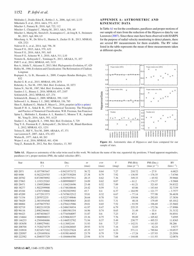
Figure A1. Astrometric data of Hipparcos and Gaia compared for oursample of stars.

Table A1. Hipparcos astrometry of the solar twins used in this work. We indicate the name of the star, equatorial sky positions, V-band apparent magnitudes,parallaxes (� ), proper motions (PM), the radial velocities (RV).

Star RA Dec. � σ� V PM (RA) PM (Dec.) RV(◦) (◦) (mas) (mas) (mag) (mas yr−1) (mas yr−1) (km s−1)

HD 2071 0.1077987647 − 0.9421973172 36.72 0.64 7.27 210.72 − 27.9 6.6823HD 8406 0.3622254703 − 0.2877530204 27.38 0.79 7.92 − 136.95 − 176.35 − 7.6766HD 20782 0.8729078992 − 0.5035957911 28.15 0.62 7.36 349.33 − 65.92 39.9666HD 27063 1.1192125265 − 0.0099900057 24.09 0.62 8.07 − 61.2 − 174.37 − 9.5868HD 28471 1.1569520864 − 1.1184218496 23.48 0.52 7.89 − 61.21 321.65 54.8322HD 38277 1.5022599908 − 0.1748188646 24.42 0.59 7.11 65.86 − 143.64 32.7339HD 45184 1.6787150866 − 0.5023025992 45.7 0.4 6.37 − 164.99 − 121.77 − 3.7577HD 45289 1.6772913373 − 0.7478632512 35.81 0.32 6.67 − 77.14 777.98 56.4638HD 71334 2.207072235 − 0.5223749846 26.64 0.78 7.81 139.04 − 292.03 17.3836HD 78429 2.3851954548 − 0.7590858065 26.83 0.51 7.31 48.18 179.49 65.1012HD 88084 2.6578675783 − 0.2704215986 29.01 0.65 7.52 − 93.59 − 196.69 − 23.5602HD 92719 2.8022119328 − 0.2406336934 41.97 0.47 6.79 235.35 − 172.56 − 17.8906HD 96116 2.8982366461 − 1.0081901354 16.96 0.74 8.65 31.49 − 35.4 31.3132HD 96423 2.9074038637 − 0.7744568097 31.87 0.6 7.23 87.3 − 86.9 54.8541HD 134664 3.9800988033 − 0.5390630337 23.36 0.75 7.76 99.89 − 105.82 7.6595HD 146233 4.2569404686 − 0.1460532782 71.94 0.37 5.49 230.77 − 495.53 11.8365HD 183658 5.1089279481 − 0.113692144 31.93 0.6 7.27 − 142.51 − 141.03 58.286HD 208704 5.7526274579 − 0.2210426045 29.93 0.74 7.16 32.03 62.24 3.9277HD 210918 5.8234517182 − 0.7222127624 45.35 0.37 6.23 571.11 − 789.84 − 19.0537HD 220507 6.1291695816 − 0.9198146045 23.79 0.79 7.59 − 17.24 − 157.93 23.2956HD 222582 6.2040357329 − 0.1044664586 23.94 0.74 7.68 − 144.88 − 111.93 12.0876

MNRAS 467, 1140–1153 (2017)

Phylogeny in the solar neighbourhood 1153

A1 Hipparcos and Gaia

While our analysis was being performed, the first data release ofGaia became public (Gaia Collaboration et al. 2016). Here wecompare the astrometric data of both missions in Fig. A1. In the left-hand panels we show the ratio of the proper motions and parallaxesof Gaia and Hipparcos in separate panels, and each star is indicatedin the x-axis. We can see that the differences between both areusually within 10 per cent, except few cases such as HD 96116,whose proper motion in RA has a difference of 30 per cent. Theright-hand panels show the ratio of the errors of these quantitiesin separate panels. Here we see how Gaia data is on general threetimes more accurate in the derived parallaxes, and up to 20 timesmore accurate in proper motions.

While this comparison would suggest to use Gaia data insteadof Hipparcos, we caution here that we do not have Gaia astrometry

for all the stars in our sample. Since we have solar twins only, wecould have applied the twin method (Jofre et al. 2015b) to determineparallaxes of the resting stars not contained in Gaia. However, inour analysis we require proper motions that are best measured by anastrometric mission. Therefore, to keep our analysis homogeneousand complete, we decided to use the Hipparcos astrometry for ouranalysis of kinematics of stars. As we did not find anything unusualfrom the kinematic behaviour of our stars, we believe that reducingthe data set to consider Gaia data has not a favourable impact norchanges the conclusions of our work.

Using the data of Table A1, i.e. the astrometry of Hipparcosand the RVs from HARPS, we calculated the actions and the totalvelocity of the stars as described in Section 3.2. These values arelisted in Table A2, together with the ages as derived by Nissen(2016) for completeness.

Table A2. Galactic coordinates, total velocities, actions and ages of the stars used in our sample. Ages are taken from Nissen (2016), while other propertiesare determined from the astrometry of Table A1 as described in Section 3.2.

Star R z U V W Jr Jz Lz Age(kpc) (kpc) (km s−1) (km s−1) (km s−1) (kpc km s−1) (kpc km s−1) (kpc km s−1) (Gyr)

HD 2071 8.29172 0.00113 − 19.95267 − 18.63223 − 7.14419 14.91899 0.00585 − 1920.49109 3.5HD 8406 8.30762 − 0.00035 37.76446 − 11.09508 − 1.11882 6.75647 0.21467 − 1986.76341 4.1HD 20782 8.31363 0.00163 − 37.38056 − 61.41219 − 2.65999 78.45743 0.12547 − 1570.39096 8.1HD 27063 8.33342 0.00096 28.59609 − 16.04689 − 18.43578 3.46062 0.70879 − 1951.65914 2.8HD 28471 8.29683 0.00392 − 53.89275 − 25.00513 − 62.07675 55.17953 28.08048 − 1870.88032 7.3HD 38277 8.33184 0.00262 − 7.98824 − 42.68783 − 11.25881 27.42507 0.07784 − 1730.0909 7.8HD 45184 8.31146 0.00209 10.02202 5.31122 − 18.37438 5.65876 0.68668 − 2124.07984 2.7HD 45289* 8.30851 0.00293 − 115.57143 − 22.89469 − 3.77961 205.68372 0.05632 − 1892.0283 9.4HD 71334 8.3128 0.00423 47.27097 − 36.36525 − 8.19526 27.75369 0.01968 − 1777.03046 8.8HD 78429 8.3028 0.00447 − 22.35954 − 62.31564 30.54011 62.0256 11.90181 − 1561.62639 8.3HD 88084 8.30748 0.00341 10.91872 − 0.78358 − 41.25848 2.60847 8.91765 − 2072.37971 5.9HD 92719 8.30281 0.00222 34.73916 9.3428 − 10.60875 14.70023 0.09766 − 2154.85832 2.5HD 96116 8.28099 0.00673 21.61917 − 25.8706 − 4.33059 6.63941 0.05597 − 1857.59697 0.7HD 96423 8.29279 0.00355 29.72398 − 49.04196 7.4871 33.82754 1.34169 − 1667.99685 7.3HD 134664 8.2642 0.00198 18.77267 − 3.22958 − 23.82393 1.42554 1.73021 − 2041.25362 2.4HD 146233 8.28791 − 0.00012 27.17963 − 14.42555 − 22.1416 2.48326 1.33952 − 1954.43792 4.0HD 183658 8.27389 − 0.00194 65.03352 6.90413 − 2.41432 39.79151 0.11846 − 2128.34777 5.2HD 208704 8.28359 − 0.0019 − 5.84723 9.76923 − 2.99267 14.57429 0.09451 − 2153.53487 7.4HD 210918* 8.28735 0.00004 − 47.58932 − 91.6203 − 8.57114 155.99919 0.00903 − 1314.04448 9.1HD 220507* 8.28179 0.0013 20.30581 − 32.88105 − 7.00157 11.95045 0.02781 − 1799.71119 9.8HD 222582 8.29731 − 0.00225 36.52928 − 0.67894 − 11.23786 7.96257 0.10894 − 2071.02691 7.0Sun 8.3 0.014 0 0 0 4.68053 0.28028 − 2076.992 4.5

This paper has been typeset from a TEX/LATEX file prepared by the author.

MNRAS 467, 1140–1153 (2017)