Cosmological Small-scale Structure: The Formation of The First Stars, Galaxies, and Globular Clusters by Alexander L. Muratov A dissertation submitted in partial fulfillment of the requirements for the degree of Doctor of Philosophy (Astronomy and Astrophysics) in The University of Michigan 2013 Doctoral Committee: Associate Professor Oleg Gnedin, Chair Professor August Evrard Professor Mario Mateo Associate Professor Eric Bell Associate Professor Mateusz Ruszkowski
Transcript
Cosmological Small-scale Structure: The Formationof The First Stars, Galaxies, and Globular Clusters
by
Alexander L. Muratov
A dissertation submitted in partial fulfillmentof the requirements for the degree of
Doctor of Philosophy(Astronomy and Astrophysics)in The University of Michigan
2013
Doctoral Committee:
Associate Professor Oleg Gnedin, ChairProfessor August EvrardProfessor Mario MateoAssociate Professor Eric BellAssociate Professor Mateusz Ruszkowski
were performed with 0.5h−1 and 0.25h−1 Mpc comoving boxes to explore the effects of
mass resolution (hereby referred to as H Mpc and Q Mpc runs, respectively). The details
for each run performed in our simulation suite are presentedin Section 2.2.3. Numbers
quoted in this paragraph, as well as Sections 2.2.1 and 2.2.2refer to our baseline 1h−1 Mpc
runs. These runs start with a 2563 root grid, which sets the DM particle mass tomDM =
5.53× 10³M⊙ and the base comoving resolution of 5.56 kpc. We employ Lagrangian
refinement criteria, refining cells when the DM mass approximately doubles compared
to the initial mass in the cell, specifically, when it exceeds2×mDM × ΩmΩDM
× 0.8, or the
gas density surpasses an approximately equivalent value modulated by the cosmic baryon
fraction 0.3×mDM × ΩmΩDM
×0.8. In both refinement conditions, the extra factor of 0.8 is
the split tolerance. We use a maximum of 8 additional levels of refinement, giving us a
final resolution of 106h−1/256/28 ≈ 22 comoving pc. Since we are studying high-redshift
galaxies, it is important to note that this translates to about 2 physical pc at the endpoint
of our simulations,z = 9, and 1 physical pc atz = 20 when the first stars begin to form.
This spatial resolution is sufficient to capture the detailed multi-phased structure of the
interstellar medium (ISM) (e.g. Ceverino & Klypin 2009).
In order to simulate several representative regions of the universe, we employ the "DC
mode" formulation presented in Sirko (2005) and Gnedin et al. (2011). Running simula-
tions with different DC modes allows us to sample cosmologically over- and under-dense
regions without actually changing the total mass within each box. A single parameter∆DC,
which is constant at all times for a given simulation box, represents the fundamental scale
of density fluctuations present in the box. At sufficiently early times, when perturbations
on the fundamental scale of the box are in the regime of lineargrowth,∆DC is related to the
overdensity,δDC(a) ≡ D+(a)∆DC, whereD+ is the linear growth factor. The expansion rate
26
of the individual box relates to the expansion rate of the universe by the following relation,
which is Equation 3 of Gnedin et al. (2011):
abox =auni
[1+∆DCD+(auni)]1/3 , (2.1)
where abox is the local scale factor of the simulation box, whileauni is the global ex-
pansion factor of the universe. For this study, we have used three different setups with
∆DC = −2.57,−3.35, and 4.04, labeled ’Box UnderDense−’, ’Box UnderDense+’ and ’Box
OverDense’, respectively. At the endpoint of our simulations, z = 9, these values trans-
late to overdensities ofδDC = −0.257,−0.335, and 0.404, respectively. Boxes UnderDense−
and UnderDense+ have negative DC modes, implying they are underdense regions of the
universe. However, while Box UnderDense− is representative of a void, and hosts only
low-mass galaxies which collapse relatively late, Box UnderDense+ hosts the first star-
forming galaxy among all three simulation boxes. This galaxy is also more massive than
any of those in Box OverDense untilz≈ 13.
Box OverDense hosts several massive star-forming galaxieswhich statistically domi-
nate the sample of simulated galaxies. The H Mpc and Q Mpc boxes used∆DC = 5.04
and 6.11, respectively. These runs are primarily designed to explore the earliest possible
epoch of Pop III star formation, tracing only the most overdense regions with even higher
mass resolution. None of our simulations continue pastz= 9, as the boxes are too small to
capture the nonlinear growth of large-scale modes at later epochs.
We construct catalogs of halo properties from simulation outputs using the profiling
routine described in Zemp et al. (2012). We take the virial radius,Rvir , as the distance from
the center of a halo which encloses a region that has an overdensity of 180 with respect to
the critical density of the universe.
2.2.1 Population II star formation
Following Gnedin et al. (2009) and Gnedin & Kravtsov (2011),we set the threshold for
Pop II star formation in a gas cell when the fraction of molecular hydrogen exceeds the
threshold fH2 ≡ 2nH2/nH = 0.1. Tests described in the above studies showed that the ex-
27
act value of this threshold was not important for overall star formation rates, but mainly
regulated the number and mass of stellar particles produced. The simulations performed
in that study employed a non-zero floor (minimum value) of thedust-to-gas ratio in cells,
which was meant to account for unresolved pre-enrichment. Since our current simulations
spatially resolve regions where the first stars are expectedto form, it is unnecessary and
inappropriate to use such a floor. This means that in our runs,prior to the metal feedback
from the first generation of stars, only primordial chemistry is used inH2 formation reac-
tions. We find that such primordial reactions with our resolution do not yield molecular
fractions fH2 > 0.01 on relevant timescales. Therefore, in order to form the first (Pop III)
generation of stars, a separate prescription is required and is outlined in the next section.
In cells where the molecular fraction exceeds thefH2 threshold, Pop II stellar particles
are formed with a statistical star formation delay,dtSF = 107 yr, implemented by drawing
a random number,P, between 0 and 1, and forming stars only ifP > exp(
− dtdtSF
)
, where
dt is the length of the timestep at the cell’s refinement level. Each particle represents a
stellar population with a Miller & Scalo (1979) IMF from 0.1M⊙ to 100 M⊙. The mass of
a stellar particle is determined by the following the relation:
ρ∗ =ǫ f f
τSFρH2. (2.2)
The star formation efficiency per free-fall time is set toǫ f f = 0.01, based on recent results of
Krumholz et al. (2012). We use a constant star formation timescaleτSF = 8.4×10⁶ yr cor-
responding to the free-fall time at hydrogen number densitynH = 50 cm−3. This approach
differs from Gnedin & Kravtsov (2011), where the timescale was computed by using the
physical density of molecular clouds. However, we find that in our simulations the density-
dependent timescale instills a strong resolution dependence on the star formation rate. Pop
II stellar particles are treated as statistical ensembles of stars for which the appropriate
metal yield and fraction of stars to go supernovae is computed by integration of the IMF.
The number of SN II explosions is 75 per 104M⊙ formed, while the amount of SN II metals
generated by a stellar particle is 1.1% of its initial mass. Each supernova releases 2×1051
erg thermal energy which is deposited over the course of 107 yr. Following the notation of
28
Hummels & Bryan (2012), this implies fraction of the rest mass energy of stars which is
available for thermal SNe feedback isESN/Mc2 = 8.4×10⁻⁶. This value is relatively high,
but consistent with values chosen by other researchers (Hummels & Bryan, 2012).
2.2.2 Population III star formation
Formation criteria
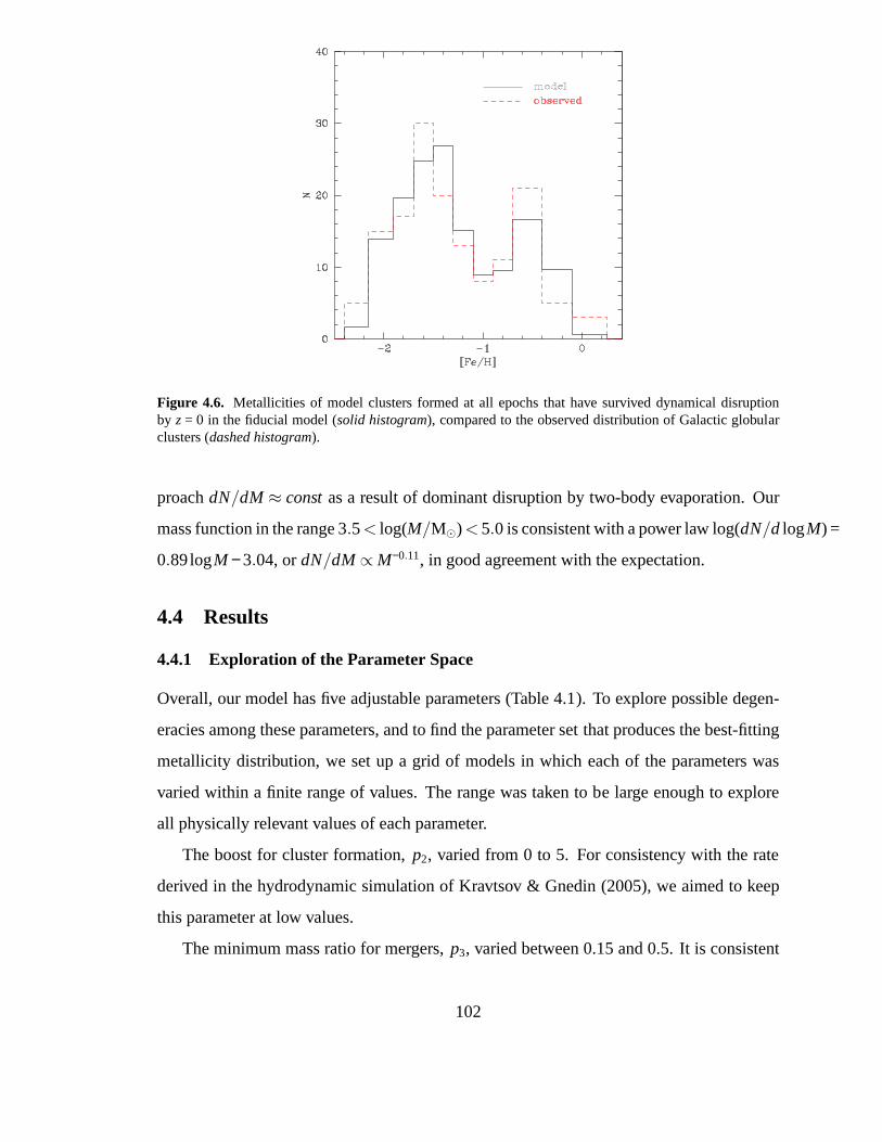
We model the formation of Pop III stars based on criteria derived from simulations of Abel
et al. (2002). These authors showed that once the core density of a proto-cloud reached
1000 cm−3, further collapse to a massive stellar object was imminent.Analyzing their
results, we found that for gas at any given densitynH past this threshold, the time of collapse
to a stellar core is approximately six times the free-fall time for that density, 6t f f (nH). This
collapse time is 9 Myr fornH = 1000 cm−3 and scales asn−1/2H . For our fiducial runs, we
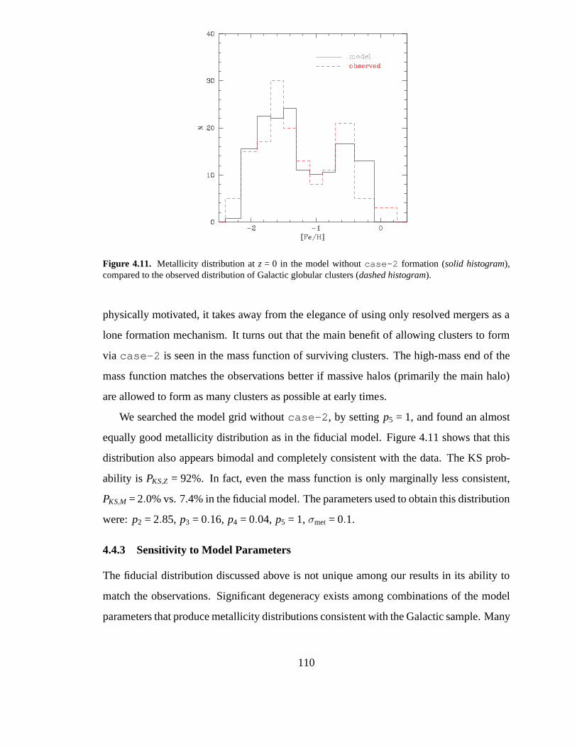
usenH,min = 10000 cm−3 as the threshold anddtSF = 2.8 Myr as the statistical star formation
delay, simulating the collapse time. This value is lower than the one used for Pop II stars.
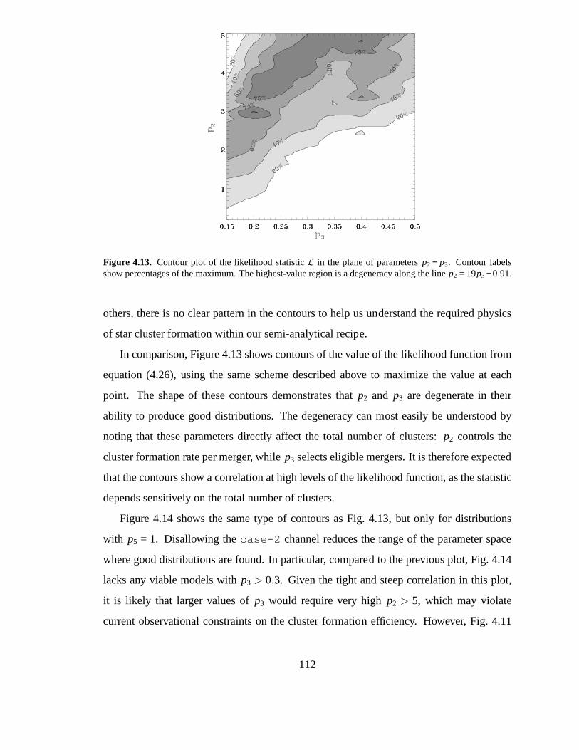
This density threshold value was chosen to ensure Pop III stars would form primarily when
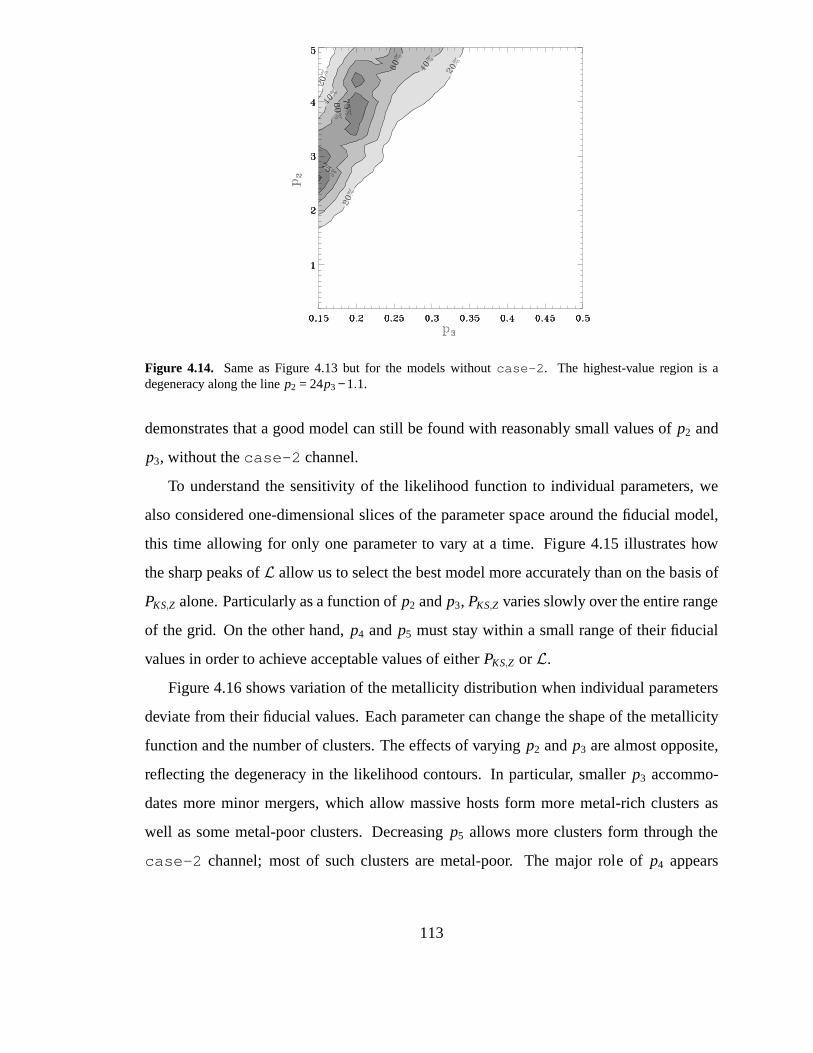
cells have been maximally refined, but is low enough such thatthe collapsing gas clouds
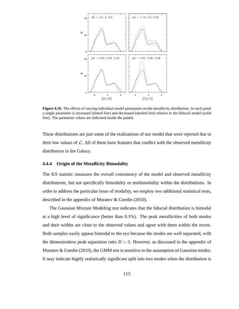
are still fully resolved in our simulations. Further discussion is presented in Section 2.2.3.
We also set a threshold for the minimum fraction of molecularhydrogen at 10−3 to
reflect that primordial gas clouds must cool primarily via ro-vibrational transitions ofH2
to form the first stars (Couchman & Rees, 1986; Tegmark et al., 1997). The precise value
of this threshold is rather arbitrary, as we do not attempt tomodel the actual chemistry of
stellar core formation. We have chosen this value because itis lower than, but close to
the typical value for the molecular hydrogen fraction in cold, dense primordial gas around
z= 20, which we have found empirically to be 2×10⁻³ (see Section 2.2.3 and Figure 2.3). A
minimum threshold for molecular fraction ensures that theH2-dissociating Lyman Werner
radiation from recently-formed Pop III stars will realistically suppress further Pop III star
formation in the region.
Pop III stars form in gas that has metallicity log10Z/Z⊙ < −3.5. This threshold is
chosen to match the critical metallicity discovered by Bromm et al. (2001a), and has held
up in later studies (Smith et al., 2009). Though the exact value of this critical metallicity
29
is still uncertain and can be affected by the presence of dust(Omukai et al., 2005), we find
that it is not very important as the majority of Pop III stars form in truly primordial, or
nearly primordial gas. Compiling all of our simulations, we found that only ~10% of Pop
III stars form with log10Z/Z⊙ > −5.
We summarize the formation criteria for Pop III stars with the following set of equa-
tions,
nH > nH,min = 104 cm−3
fH2 > fH2,min = 10−3
log10Z/Z⊙ < −3.5. (2.3)
Values given for each variable represent the fiducial choices.
IMF and supernova feedback
The IMF of Pop III stars is currently a hotly debated and active area of research. It is
still unclear whether the high Jeans mass of primordial gas results in a top-heavy IMF as
predicted by early studies (Abel et al., 2002; Bromm et al., 1999; Yoshida et al., 2003),
or if the angular momentum and radiative effects during infall can fragment the cloud and
generate relatively low-mass cores (Greif et al., 2011; Stacy et al., 2012; Hosokawa et al.,
2011; Clark et al., 2011). It is even likely that the Pop III IMFcan be considerably variable
depending on environment (O’Shea & Norman, 2007) and ionization state of the collapsing
gas (Yoshida et al., 2007). We choose not to explore various analytic forms for the IMF,
as constraining it is beyond the scope of this paper. Instead, we consider that the main
way by which the Pop III IMF can influence galaxy formation, incontrast to the known
Pop II IMF, is by enhancing the output of ionizing radiation and the number and intensity
of supernovae. In particular, PISNe, which are hypothetically plausible from stars in the
mass range 140− 260M⊙ (or for lower masses if rotation is considered, see e.g. Stacy
et al. 2013), would potentially be dramatic singular eventsin the evolution of any galaxy
(Bromm et al., 2003; Whalen et al., 2008). To account for the occurrence of PISNe we
use two different particle masses for Pop III stars. Every newly formed Pop III stellar
30
particle is randomly assigned to be either a 170M⊙ star, which is to explode in a PISN,
or 100M⊙ star, which only generates a mild explosion before collapsing into a black hole
(Heger & Woosley, 2002, 2010). The proportion of these two types of particle mass and
fate is governed by a single parameter,PPISN, which is the fraction of PISNe progenitors
(170M⊙ stars) that form when the Pop III star formation criteria aremet. In our fiducial
runs, we setPPISN = 0.5. This value was chosen to test the maximum possible impact of
PISNe on galaxy evolution, and probably represents the mosttop-heavy the primordial IMF
can possibly be. Since the atmospheres of Pop III stars are free of metals, they are unable
to drive stellar winds and therefore do not enrich the ISM in any way other than through
supernovae. Pop III stars which have masses too low to produce SNe are ignored in our
model.
For our fiducial value ofnH,min (as well as all other parameters considered in Section
2.2.3), we found that the gas mass in a maximally refined cell at z≈ 20 is sometimes not
sufficient to form a 170M⊙ star. Therefore, we prevent further refinement in metal-free
cells that havenH > 0.5nH,min and whose splitting would leave insufficient mass to form the
star. Through tests, we have checked that this refinement restriction never artificially slows
down Pop III star formation. It becomes especially relevantin the super-Lagrangian runs
discussed in Section 2.2.3 and in the H and Q Mpc boxes which inherently have very high
resolution.
The PISN from a 170M⊙ star releases 27× 1051 erg of thermal energy, as well as
80M⊙ of metals into the ISM (Heger & Woosley, 2002). As suggested by Wise & Abel
(2008), we use a delay of 2.3 Myr from the formation of a 170M⊙ particle to its PISN
event, representing the main sequence lifetime of this typeof star (Schaerer, 2002). After
the supernova goes off, the cell which hosts it often winds upwith super-solar metallicity.
The cooling functions employed in our code are not accurate for these high-temperature
high-metallicity conditions associated with the early phases of supernova remnants. We
found that while the blastwave expanded regardless of whether or not cooling was turned
on, the inner regions of the supernova remnant overcooled. We therefore turned off all
metal cooling for gas at temperatures higher than 104K. According to the models of Heger
& Woosley (2002), a 170M⊙ star is completely disrupted by its PISN event, and all gas
31
mass from the stellar interior would be ejected into the ISM leaving no remnant. The ejecta
then consists of 80M⊙ of metals from the core, as well as the primordial envelope which
is 22M⊙ of He and 68M⊙ of H.
A 100M⊙ star does not explode as a PISN, but its actual fate is still uncertain and
depends on the details of the stellar rotation and magnetic structure (Heger & Woosley,
2010). Before undergoing core collapse, such a star would experience thermonuclear pair-
instability pulses that would eject the outer layers of H andHe, with possible traces of the
elements C, N, and O. The energy released in such pulses is of the order or smaller than
the energy of a normal SN type II. If the remaining core has enough rotation to trigger
a gamma-ray burst in the collapsar model (Woosley & Heger, 2012), it may then lead to
a powerful explosion with over 1052 erg of energy and the ejection of significant mass of
metals. Without rotation, the core may drive a weak collapsar explosion or no explosion at
all, when all the remaining mass recollapses. Given these uncertainties, and to contrast with
the case of a full PISN explosion for the 170M⊙ stars, for the 100M⊙ stars we assume that
no substantial metals are deposited into the ISM and that thereleased energy corresponds
to a standard SN type II. About 50M⊙ of gas is released into the ISM, while also leaving
behind a remnant black hole of ~50M⊙.
To prevent artificial radiative losses, PISN energy and massejecta are distributed within
a sphere of constant density, with a radius 1.5 cell lengths,centered at the middle of the
PISN host cell. Each of the 27 cells within such a sphere, consisting of the star’s host cell
and its immediate neighbors, receive a dose of energy and metal-rich gas proportional to
the actual volume of the cell contained within the sphere. This prescription is physically
motivated as we found that our typical timestep (about 450 yr) is too coarse compared to the
typical timescale of the early free expansion phase of the SNremnant. For example, it takes
the ejecta ~500 yr to traverse half of the typical Pop III starhost cell length (4.5 pc) atz~20
if it travels at the free-expansion velocity. This velocityis computed here by assuming that
all of the PISN energy of 27×1051 erg goes into kinetic energy of the ejecta. In practice,
we found that this model did not significantly affect the geometry of the blastwave relative
to simulations where we injected the metals and energy into asingle cell.
32
Radiative feedback
In addition to the supernova feedback, all Pop III stars haveenhanced radiative feedback
relative to Pop II counterparts, due to the lack of metals in their atmospheres (Schaerer,
2002). We use the same spectral shape for the ionizing feedback of all stellar particles
(the Pop II SED from Figure 4 of Ricotti et al. 2002a), which has a characteristic energy
of 21.5 eV for ionizing photons, however we enhance the radiative output of Pop III stars
by a factor of 10 relative to Pop II, following Wise & Cen (2009). After a Pop III stellar
particle undergoes supernova, radiative feedback from thestar is completely shut off. On
the other hand, Pop II stellar particles shine according to alight curve fit from Starburst
99 model results (Leitherer et al., 1999). This light curve consists of a flat component for
the first 3×10⁶ yr, followed by a steep power-law falloff. Radiative feedback from Pop
II stellar particles becomes insignificant after 3×10⁷ yr. Since Pop II stars shine longer
than both types of Pop III stars, the factor of 10 radiative enhancement does not translate
into a proportionally higher number of ionizing photons perlifetime. Pop II stars emit
6,600 ionizing photons per stellar baryon per lifetime. In our fiducial runs, Pop III stars
emit 38,800 and 34,500 photons per baryon per lifetime for the 100M⊙ and 170M⊙ stars,
respectively.
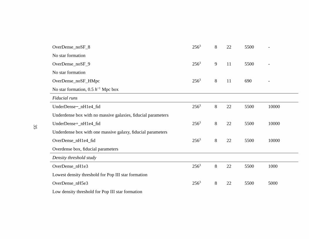
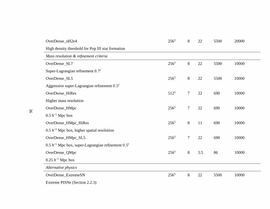
2.2.3 Convergence Study & Setting Fiducial Parameters
In this section, we describe the test runs that justify the numerical setup and the choice
of parameters for our main runs. Since the Pop III star formation recipe described above
is one of the critical components of our study, we focus on testing the key elements of
this model. In Table 1 we list the details of the simulations performed in our suite. Box
OverDense has many more potential sites for Pop III star formation than the other 1h−1
Mpc boxes, and therefore serves as the best testing ground. It is important to keep in mind
that while every parameter we test has an effect on Pop III star formation, the most drastic
differences between the simulations are caused by the choice of initial conditions. The role
of cosmic variance will be explored more comprehensively inChapter 3.
33
Table 2.1: SIMULATION RUNS OFCHAPTER 2
Run Base grid ℓmax dx (pc) mDM(M⊙) nH,min(cm−3)
Description
Convergence study
UnderDense−_noSF_7 2563 7 44 5500 -
No star formation
UnderDense−_noSF_8 2563 8 22 5500 -
No star formation
UnderDense−_noSF_9 2563 9 11 5500 -
No star formation
UnderDense+_noSF_7 2563 7 44 5500 -
No star formation
UnderDense+_noSF_8 2563 8 22 5500 -
No star formation
UnderDense+_noSF_9 2563 9 11 5500 -
No star formation
OverDense_noSF_7 2563 7 44 5500 -
No star formation
34
OverDense_noSF_8 2563 8 22 5500 -
No star formation
OverDense_noSF_9 2563 9 11 5500 -
No star formation
OverDense_noSF_HMpc 2563 8 11 690 -
No star formation, 0.5h−1 Mpc box
Fiducial runs
UnderDense−_nH1e4_fid 2563 8 22 5500 10000
Underdense box with no massive galaxies, fiducial parameters
UnderDense+_nH1e4_fid 2563 8 22 5500 10000
Underdense box with one massive galaxy, fiducial parameters
OverDense_nH1e4_fid 2563 8 22 5500 10000
Overdense box, fiducial parameters
Density threshold study
OverDense_nH1e3 2563 8 22 5500 1000
Lowest density threshold for Pop III star formation
OverDense_nH5e3 2563 8 22 5500 5000
Low density threshold for Pop III star formation
35
OverDense_nH2e4 2563 8 22 5500 20000
High density threshold for Pop III star formation
Mass resolution & refinement criteria
OverDense_SL7 2563 8 22 5500 10000
Super-Lagrangian refinement 0.7ℓ
OverDense_SL5 2563 8 22 5500 10000
Aggressive super-Lagrangian refinement 0.5ℓ
OverDense_HiRes 5123 7 22 690 10000
Higher mass resolution
OverDense_HMpc 2563 7 22 690 10000
0.5h−1 Mpc box
OverDense_HMpc_HiRes 2563 8 11 690 10000
0.5h−1 Mpc box, higher spatial resolution
OverDense_HMpc_SL5 2563 7 22 690 10000
0.5h−1 Mpc box, super-Lagrangian refinement 0.5ℓ
OverDense_QMpc 2563 8 5.5 86 10000
0.25h−1 Mpc box
Alternative physics
OverDense_ExtremeSN 2563 8 22 5500 10000
Extreme PISNe (Section 2.2.3)
36
OverDense_ExtremeRad 2563 8 22 5500 10000
Extreme Pop III radiation field (Section 2.2.3)
OverDense_LowMass 2563 8 22 5500 10000
Pop III IMF and feedback mirror Pop II (Section 2.2.3)
Column 1.) Name of the run;
2.) Base grid, number of DM particles, number of root cells;
3.) Maximum number of additional levels of refinement;
4.) Minimum cell size at the highest level of refinement in comoving pc;
5.) DM particle mass in M⊙;
6.) Minimum H number density for Pop III star formation in cm−3;
7.) Further description of the run. sideways
37
Density threshold for Pop III star formation
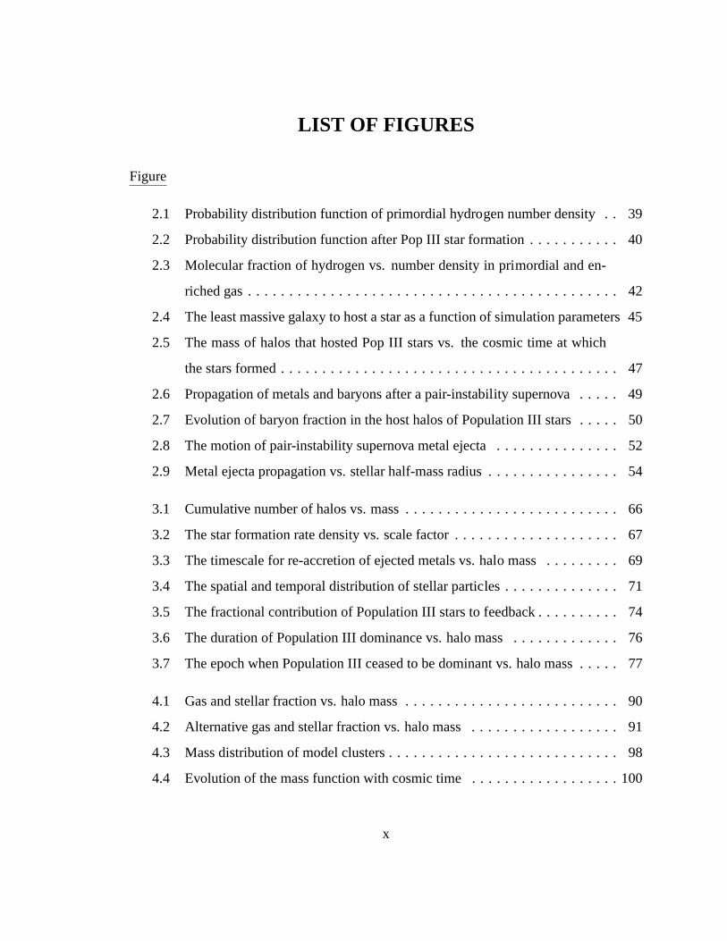
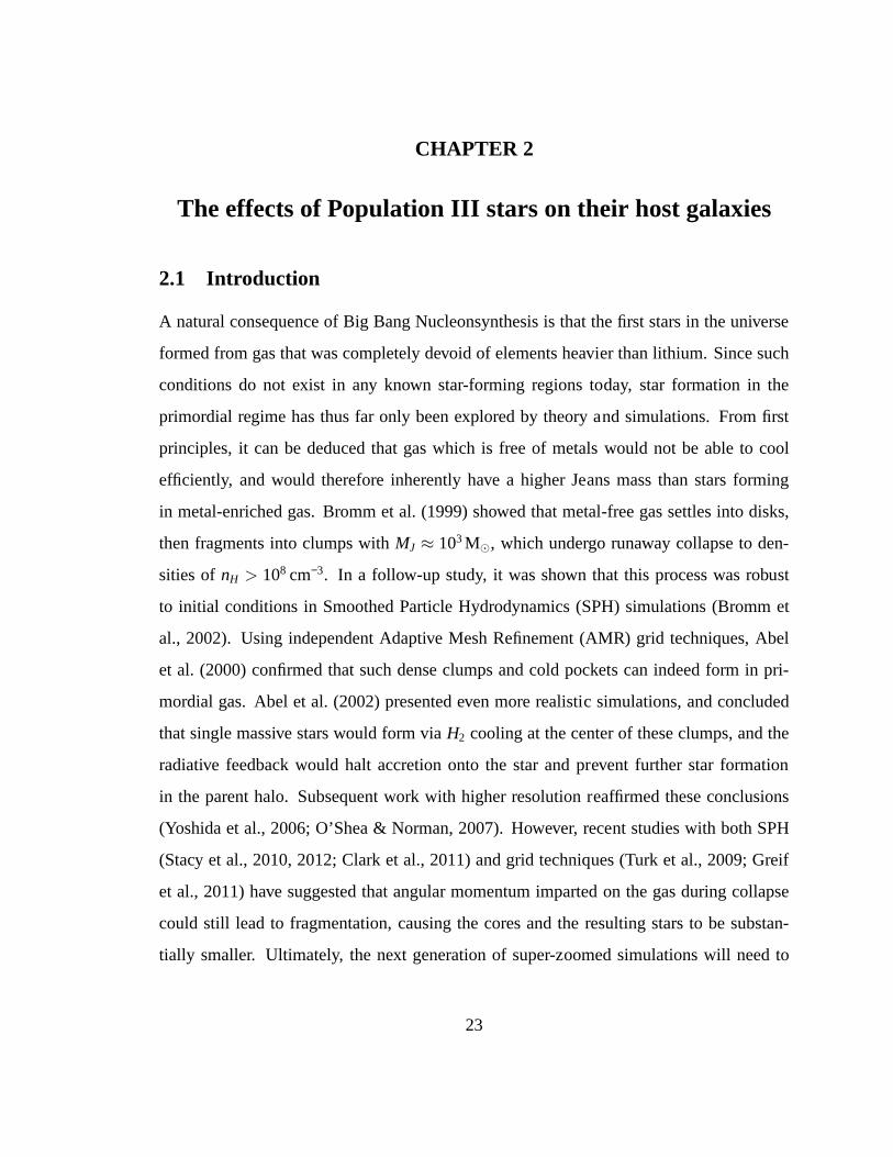
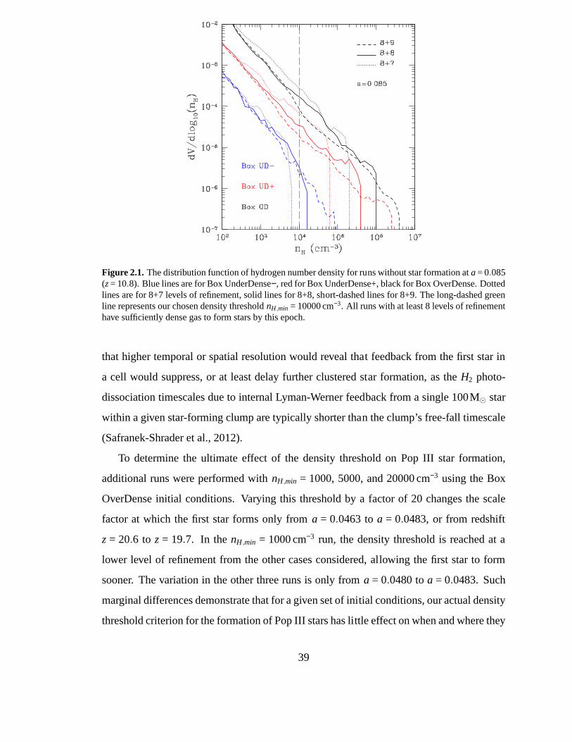
First, we choose an appropriate value for the density threshold for creating Pop III stars.
In Figure 2.1, we examine the high-density end of the volumetric probability distribution
function (PDF) of the hydrogen number density ata = 0.085 (z = 10.8). In order to test
the properties of the primordial gas from which the first stars form, we ran a special set
of simulations with no star formation or chemical enrichment (runs OverDense_noSF_8,
UnderDense+_noSF_8, UnderDense−_noSF_8, as well as additional versions of each with
one more and one fewer maximum level of spatial refinement). Though the total mass
of gas in each box is the same, only gas in the most massive halos has collapsed to this
density regime, meaning that the PDFs are very sensitive to the number and nature of such
halos. The PDFs of Box OverDense and UnderDense+ are offset by a factor of ~5 at all
densities, while the UnderDense− box is offset from Box UnderDense+ by another factor
of ~5. This difference is also seen in the maximum density achieved in each box. For our
fiducial resolution of 8+8 levels, all three boxes are able toreach a density of at least 10000
cm−3 by a = 0.085, giving us enough time to study star formation in every box before our
stopping point ofa = 0.1.
Based on these results, we chosenH,min = 10000 cm−3 as our fiducial value for the den-
sity threshold. In addition to the constraints obtained from the PDF, other considerations
went into this selection. A lower value would suffice to meet our proto-cloud collapse
criteria, but would result in all Pop III stellar particles forming before cells are maximally
refined. Such an outcome is poor practice in hydrodynamic simulations, as subgrid physics
is being invoked on scales where the resolution is still goodenough to self-consistently
capture relevant physical processes. On the other hand, using a higher threshold would
allow the maximally refined cells to reach densities beyond the resolving power of the sim-
ulation. When such conditions are reached, either further refinement or subgrid physics
should already be in use. In addition, using a higher densitythreshold in our test runs often
led to Pop III stars forming in bursts (in the same timestep, in neighboring cells). We do
not speculate here whether such bursts are physically plausible or not, but the scales neces-
sary to model this process properly are certainly unresolved in our simulations. We suspect
38
Figure 2.1.The distribution function of hydrogen number density for runs without star formation ata= 0.085(z= 10.8). Blue lines are for Box UnderDense−, red for Box UnderDense+, black for Box OverDense. Dottedlines are for 8+7 levels of refinement, solid lines for 8+8, short-dashed lines for 8+9. The long-dashed greenline represents our chosen density thresholdnH,min = 10000 cm−3. All runs with at least 8 levels of refinementhave sufficiently dense gas to form stars by this epoch.
that higher temporal or spatial resolution would reveal that feedback from the first star in
a cell would suppress, or at least delay further clustered star formation, as theH2 photo-
dissociation timescales due to internal Lyman-Werner feedback from a single 100M⊙ star
within a given star-forming clump are typically shorter than the clump’s free-fall timescale
(Safranek-Shrader et al., 2012).
To determine the ultimate effect of the density threshold onPop III star formation,
additional runs were performed withnH,min = 1000, 5000, and 20000 cm−3 using the Box
OverDense initial conditions. Varying this threshold by a factor of 20 changes the scale
factor at which the first star forms only froma = 0.0463 toa = 0.0483, or from redshift
z = 20.6 to z = 19.7. In thenH,min = 1000 cm−3 run, the density threshold is reached at a
lower level of refinement from the other cases considered, allowing the first star to form
sooner. The variation in the other three runs is only froma = 0.0480 toa = 0.0483. Such
marginal differences demonstrate that for a given set of initial conditions, our actual density
threshold criterion for the formation of Pop III stars has little effect on when and where they
39
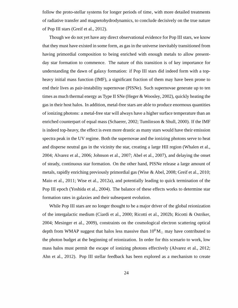
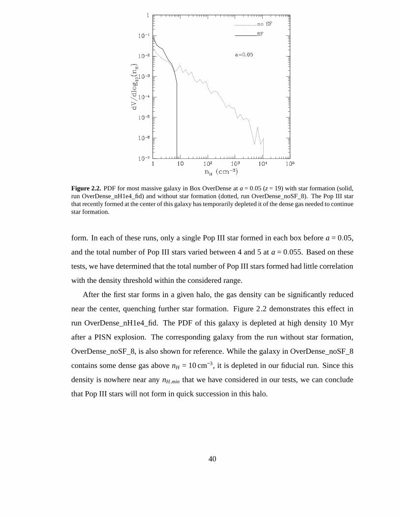
Figure 2.2. PDF for most massive galaxy in Box OverDense ata = 0.05 (z= 19) with star formation (solid,run OverDense_nH1e4_fid) and without star formation (dotted, run OverDense_noSF_8). The Pop III starthat recently formed at the center of this galaxy has temporarily depleted it of the dense gas needed to continuestar formation.
form. In each of these runs, only a single Pop III star formed in each box beforea = 0.05,
and the total number of Pop III stars varied between 4 and 5 ata = 0.055. Based on these
tests, we have determined that the total number of Pop III stars formed had little correlation
with the density threshold within the considered range.
After the first star forms in a given halo, the gas density can be significantly reduced
near the center, quenching further star formation. Figure 2.2 demonstrates this effect in
run OverDense_nH1e4_fid. The PDF of this galaxy is depleted at high density 10 Myr
after a PISN explosion. The corresponding galaxy from the run without star formation,
OverDense_noSF_8, is also shown for reference. While the galaxy in OverDense_noSF_8
contains some dense gas abovenH = 10 cm−3, it is depleted in our fiducial run. Since this
density is nowhere near anynH,min that we have considered in our tests, we can conclude
that Pop III stars will not form in quick succession in this halo.
40
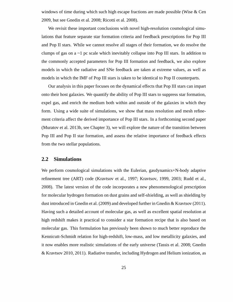
Molecular Fraction
Another component of the Pop III star formation criterion isthe requirement of a minimal
fraction of H2 in the host cell. To determine what value of theH2 threshold makes sense
in the context of these simulations, we examine the molecular fraction of hydrogen as a
function of density in the runs without star formation at theepoch (z≈ 20) when gas is
beginning to reach densities close tonH,min. Figure 2.3 shows that the molecular fraction
in primordial gas generally increases with density, but saturates abovenH ≈ 10 cm−3. The
saturation value offH2 grows slowly with time in the absence of star formation, and does
not appear to depend significantly on spatial or mass resolution. Our fiducial choice of 10−3
for the minimalH2 fraction does not exclude dense gas from forming stars in anyruns, as
long as little Lyman-Werner radiation is present.
41
Figure 2.3.Molecular fraction of hydrogen vs. number density for threeBox OverDense runs using differentresolution without star formation ata = 0.05 (z = 19, runs OverDense_noSF_9, OverDense_noSF_8, andOverDense_noSF_7 are black triangles, red circles, and purple squares, respectively). The medianH2 fractionin each density bin is indicated by a triangle, while the error bars show 25th and 75th percentile levels.At this epoch, when the first stars would normally be forming,our fiducial resolution of 8 levels has thesame molecular fraction as if we were using one more or one fewer level of refinement, and the pointsactually lie directly on top of each other fornH < 10 cm−3. Run OverDense_noSF_HMpc ata = 0.05 (greenfilled triangles) has lower values and wider spread ofH2 fraction fornH < 102 cm−3 but converges with theother runs at higher densities, demonstrating a lack of dependence on mass resolution. Also shown is runOverDense_nH1e4_fid where star formation has already takenplace bya = 0.05 (blue filled circles). Sincethe gas has been enriched by a PISN, molecular gas can form at much lower densities. Light red and light bluepoints trace out theH2 fraction in every single cell for run OverDense_noSF_8 and OverDense_nH1e4_fid,respectively.
42
Super-Lagrangian Refinement
Since we have demonstrated resolution dependence for the maximum density of gas within
a given galaxy, it is expected that refinement criteria couldplay a role in controlling when
gas in the simulation first reaches thenH,min threshold. To test this, in some of our runs
we employ super-Lagrangian (SL) refinement criteria. This approach dictates that the re-
finement threshold between subsequent levels is lowered by aconstant factor, granting
a more effective zoom-in on the densest regions at earlier times. The refinement crite-
ria in a cell can be written as 2×mDM × ΩmΩDM
×Xℓ × 0.8 for the dark matter mass, and
0.3×mDM × ΩmΩDM
×Xℓ×0.8 for the gas mass, whereℓ is the level of the cell which is to be
refined. In this formalismX = 1 implies Lagrangian refinement as described at the begin-
ning of Section 2.2. We have tried runs with very aggressive SL refinement (X = 0.5, run
OverDense_SL5) and less aggressive refinement (X = 0.7, run OverDense_SL7). Running
these simulations in Box OverDense withnH,min = 10000 cm−3, we found that the epoch at
which Pop III stars first appear is pushed back froma = 0.0478 toa = 0.0456 withX = 0.7,
and toa= 0.0435 withX = 0.5. This demonstrates that the use of SL refinement is an impor-
tant numerical tool for exploring the earliest epoch of starformation in a given simulation
box. However, using SL refinement produces an enormous number of high-level cells:
at a = 0.05, run OverDense_SL5 has a factor of 4000 more maximally refined cells than
run OverDense_nH1e4_fid. This drastic difference makes theSL simulations prohibitively
expensive soon after the first stars form.
Therefore, we use these SL runs to study Pop III star formation at the earliest possible
epochs, when the mass of the halos that hosted them was low enough for PISNe to have
their maximal effect.
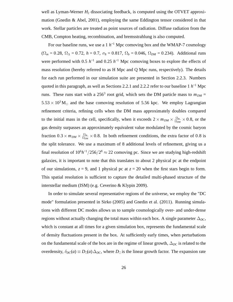
Increased Mass Resolution
We test the effects of mass resolution by setting up one run with 5123 initial grid, giving a
DM particle mass of 690M⊙. We use 7 additional levels of refinement, therefore granting
us the same maximum spatial resolution as in the fiducial 2563 run. Having consistency in
spatial resolution allows us to test the effects of mass resolution alone. All other numerical
parameters are kept consistent with run OverDense_nH1e4_fid.
43
The increased mass resolution has several immediate implications. Since we now re-
solve halos of mass 106M⊙ with over 1000 particles, we can better probe the regime where
the very first Pop III stars are expected to collapse in proto-galactic ’minihalos’. Indeed, the
epoch of formation of the first star in the box becomesa = 0.0427 in a halo of 1.5×10⁶M⊙
(compared toa= 0.0481 andMh = 7.5×10⁶M⊙ in run OverDense_nH1e4_fid). The higher
mass resolution effectively means that there is more power on the small scales responsible
for the growth of halos in this mass regime. Due to the high computational cost of this run,
we have only advanced it toa = 0.055.
The effect of increasing mass resolution is further explored through runs using the H
and Q boxes of 0.5h−1 Mpc and 0.25h−1 Mpc in size. Applying the 2563 base grid to these
boxes gives us a DM particle mass of 690M⊙ and 86M⊙, respectively. We find that the H
box (run OverDense_HMpc_HiRes) produces a Pop III star bya= 0.0456 in a halo of mass
1.5×10⁶M⊙, while the Q Mpc box (run OverDense_QMpc) does not produce one until
a = 0.0473. Using SL refinement in the HMpc box (run OverDense_HMpc_SL) allows us
to see a Pop III star forming in a 8×10⁵ M⊙ halo.
The earlier formation epochs and lower mass of halos hostingthe first stars in the
H and Q Mpc boxes, compared to the fiducial 1h−1 Mpc runs, show that it is crucial
to have high enough mass resolution to capture Pop III star formation in halos close to
106M⊙. It has been previously shown that halos less massive than this threshold will
not achieve significant enoughH2 abundances to trigger Pop III star formation at earlier
epochs (Yoshida et al., 2003). The further significance of this mass range will be explained
in our Results section. Figure 2.4 shows explicitly how varying refinement criteria, spatial
resolution, and mass resolution affected the lowest possible mass for a star-forming galaxy.
Low Mass Pop III IMF
We present one simulation, run OverDense_LowMass, which does not rely on a top-heavy
IMF for Pop III stars. The conditions for Pop III star formation in this run are similar to our
fiducial top-heavy recipe in that we use the same thresholdnH,min to determine which cells
are allowed to form stars. However, the stellar particle masses are drawn from the same
IMF as for Pop II stars. This run explores the possibility that Pop III stars were ordinary
44
Figure 2.4. The least massive galaxy to host a star in various runs vs. theminimum comoving cell sizeemployed in the run. The colors indicate the simulation box size: 1h−1 Mpc (black), 0.5h−1 Mpc (red), or0.25h−1 Mpc (blue). The shape of points indicates the refinement criterion employed in the box, with opensquares for Lagrangian refinement, filled triangles for 0.7ℓ SL refinement, and open five-pointed stars for0.5ℓ SL refinement.
low-mass objects. Whenever the density in a given cell exceeds the threshold, the star
formation rate is determined according to the following relation:
ρ∗ =ǫ f f
τSFρgas, (2.4)
whereρgas is the mass density of all gas in the cell. This relation is similar to equation 2.2,
but does not explicitly use molecular hydrogen. This modification is necessary because
primordial gas can reach densities above our star formationthreshold, but cannot become
fully molecular without the presence of dust.
Extreme Pop III Feedback
To isolate the relative impacts of the feedback effects, we ran toy simulations using exag-
gerated values for the PISN energy and ionizing photon yield. In one run, called Over-
Dense_ExtremeSN, PISNe released 270×1051 erg of thermal energy, a factor of 10 larger
than in all other runs. The extreme ionizing simulation OverDense_ExtremeRad had in-
45
stead an additional factor of 10 boost in the ionizing photonflux of Pop III stars, giving the
100M⊙ and 170M⊙ stars 388,000 and 345,000 photons per lifetime, respectively. While
these models are too strong to be consistent with any published results, using them allows
us to explore the most extreme effects of Pop III feedback.
2.3 Results
Pop III stars in our simulations begin to form in halos of massMh & 106M⊙ starting at
a ≈ 0.045 (z≈ 21.2) in accordance with expectations from prior work (Yoshidaet al.,
2003). Figure 2.5 shows the mass of host halo in which each PopIII star formed. Pop
II stars begin forming in most of these halos shortly thereafter, but are not shown in this
plot. In the 1h−1 Mpc runs, the halo mass for first star formation is close to 107M⊙.
This mass is an order of magnitude larger than that of the halos hosting the first stars
in the simulations of Wise et al. (2012a) and Greif et al. (2011), and those preferred by
theoretical considerations (Tegmark et al., 1997). Consequently, those authors also find
an earlier epoch for the formation of the first stars. Given that the extra mass resolution
granted by the H Mpc box allows us to see star formation in 106M⊙ halos, we infer that
our fiducial 1h−1 Mpc runs are not properly resolving the very first star-forming minihalos.
Rather, they are more generally simulating Pop III star formation in an early population
of galaxies. The fraction of star-forming halos in run OverDense_nH1e4_fid ata = 0.07
(z= 13.3) was only 1% in the mass range 106M⊙ < Mh < 107M⊙, but it reached 65% for
Mh > 107M⊙. In run OverDense_HMpc_HiRes, these numbers increase significantly to
15% for 106 M⊙ < Mh < 107M⊙ and 100% forMh > 107M⊙. In addition to the resolution
effects, the suppression of star formation in the 106 to 107 M⊙ range is also plausible in the
regime of a moderate Lyman-Werner background (e.g. Machacek et al. 2001; O’Shea &
Norman 2008; Safranek-Shrader et al. 2012).
It is worth noting that the ratio of star-forming galaxies inthe range 107M⊙ < Mh <
108M⊙ falls off gradually with time in run OverDense_nH1e4_fid. Itchanges from 65%
at a = 0.065 to 20% ata = 0.1, suggesting that halo mass alone is not a good proxy for
determining whether a galaxy can achieve the high density required for our Pop III star
formation criteria. One potential cause of the change is thedecreased physical spatial
46
Figure 2.5. Each Pop III star’s host halo mass at the time of formation vs.the scale factor at whichthe star formed for run UnderDense−_nH1e4_fid (blue), run UnderDense+_nH1e4_fid (red), run Over-Dense_nH1e4_fid (black), and run OverDense_HMpc_HiRes, which did not go pasta = 0.075 (green). Ad-ditional points for the halos hosting the first stars from each of the runs used for Figure 2.4 are also included,with the same color and shape scheme. In our 1h−1 Mpc runs, Pop III star formation happens almost exclu-sively in halos between 107 M⊙ and 108 M⊙. The additional mass resolution in run OverDense_HMpc_HiResmakes it possible to see that the first Pop III stars form in halos between 106 M⊙ and 107 M⊙. The averagemass of Pop III star-forming halos increases slightly with time. When multiple Pop III stars form within agalaxy in a very short time interval, points on the plot are grouped into a clustered shape.
resolution at later epochs, but according to our study of thegas in the first star-forming
galaxy shown in Figure 2.3, the factor-of-two difference inspatial resolution achieved by
using one fewer level of refinement does not preclude gas fromreaching the fiducialnH,min =
104 cm−3 threshold. The difference is more likely to be rooted in the evolution of physical
density in halos of a given mass. For halos between 107 and 108M⊙, the average matter
density within the virial radius changes from 2.5× 10⁻² M⊙ pc−3 at a = 0.065 to 6.8×
10−3M⊙ pc−3 at a = 0.1, due to the expansion of the universe. Even the density within the
central 100 pc of these halos changes from 0.73M⊙ pc−3 to 0.34M⊙ pc−3 between the same
two epochs.
Very few Pop III stars formed in halos withMh > 108M⊙, because such halos have
already been enriched to metallicities above log10Z/Z⊙ = −3.5, allowing for normal star
formation to commence. In many cases, halos withMh > 3×10⁷ M⊙ had earlier formed
47
one or more 100M⊙ Pop III stars, which shut off star formation temporarily butdid not
enrich the galactic gas, allowing it to remain pristine and continue forming Pop III stars.
Another major exception occurs in run OverDense_nH1e4_fid in a galaxy that has already
formed a significant number of Pop II stars that have in turn enriched the ISM terminating
further Pop III star formation. However ata = 0.095, this galaxy undergoes a major merger
with another massive halo, causing low-metallicity gas in the outer part of the galaxy to
collapse, thereby triggering a burst of Pop III star formation which appears as a cluster of
points withMh = 5×10⁸ on Figure 2.5. All of these stars form with metallicities around
the critical log10Z/Z⊙ = −3.5 value, suggesting that their existence is sensitive to thevalue
of this threshold and therefore should not be treated as a general result.
2.3.1 Effect of Pop III stars on their host galaxies
The strong ionizing flux of Pop III stars and enormous energy injections from PISNe have
been shown in previous work to significantly alter the ISM of their host galaxies. Here we
explore such effects during time when Pop III stars are the dominant drivers of feedback.
In Figure 2.6 we show that there is a significant variation in the potential effect of
Pop III stars on their host galaxies depending on the galaxy mass. In halos withMh <
3×10⁶M⊙, Pop III stars can temporarily evacuate the gas from the galaxy, and the metals
from PISNe are ejected past the virial radius into the intergalactic medium (IGM). On the
other hand in halos withMh > 3×10⁶M⊙, the metals are confined within the virial radius,
and there is little movement of baryons beyond the virial radius.
48
Figure 2.6. Though metals from PISNe are ejected past the virial radius,they do not stay there for long.Plotted here are the radii enclosing 80% of the metals produced in the galaxy, as well as the radii where theenclosed mass of baryons divided by the virial mass equals 80% of the universal baryon fraction. Each linerepresents a galaxy as it evolves in time, beginning at the epoch when the first star forms. Within 50 Myr ofthe PISN event (denoted by five-pointed stars), most of the gas and metals have begun to recollapse, or areat least enclosed within the virial radius once again. The maximum extent of metal propagation is stronglyregulated by galaxy mass. The distance between two points oneach line corresponds to 10 Myr.
49
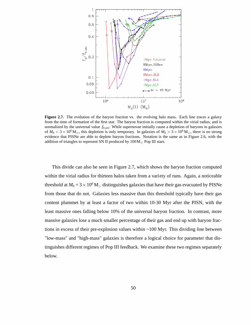
Figure 2.7. The evolution of the baryon fraction vs. the evolving halo mass. Each line traces a galaxyfrom the time of formation of the first star. The baryon fraction is computed within the virial radius, and isnormalized by the universal valuefb,uni. While supernovae initially cause a depletion of baryons in galaxiesof Mh < 3×10⁶ M⊙, this depletion is only temporary. In galaxies ofMh > 3×10⁶ M⊙, there is no strongevidence that PISNe are able to deplete baryon fractions. Notation is the same as in Figure 2.6, with theaddition of triangles to represent SN II produced by 100M⊙ Pop III stars.
This divide can also be seen in Figure 2.7, which shows the baryon fraction computed
within the virial radius for thirteen halos taken from a variety of runs. Again, a noticeable
threshold atMh = 3×10⁶M⊙ distinguishes galaxies that have their gas evacuated by PISNe
from those that do not. Galaxies less massive than this threshold typically have their gas
content plummet by at least a factor of two within 10-30 Myr after the PISN, with the
least massive ones falling below 10% of the universal baryonfraction. In contrast, more
massive galaxies lose a much smaller percentage of their gasand end up with baryon frac-
tions in excess of their pre-explosion values within ~100 Myr. This dividing line between
"low-mass" and "high-mass" galaxies is therefore a logical choice for parameter that dis-
tinguishes different regimes of Pop III feedback. We examine these two regimes separately
below.
50
Dependence on halo mass
To further understand how halo mass can determine the effectiveness of Pop III stellar
feedback, we examine the structural evolution of several galaxies in different mass regimes.
First, we examine a relatively low-mass galaxy from run OverDense_HMpc_HiRes,
which is shown by the black line that extends toM ≈ 107M⊙ in Figures 2.6 and 2.7. The
first star (of 170M⊙) forms when the mass of the halo is 1.7×10⁶M⊙. Within 20 Myr of
its formation, the PISN has blasted metals out beyond 1 kpc from the galactic center (or
4Rvir at this epoch), and the baryon fraction has dipped tofb/ fb,uni ≈ 0.15. However, soon
after this point the baryon fraction begins to grow again, and the virial radius increases
enough to enclose a larger fraction of the expelled gas and metals.
At t = 139 Myr after the first PISN (the halo mass is now 9×10⁶M⊙), the galaxy has re-
gained ~37% of the PISNe metals. The baryon fraction is over half of the universal value.
It will still take more time for this galaxy to completely recover from the explosion, but
there is considerable evidence from Figure 2.6 that metals and baryons in general are flow-
ing in rather than out of the galaxy. Another sign of recoveryis that Pop II star formation
has commenced within the galaxy, as it now contains 4 Pop II stellar particles (which still
contribute little to the metal budget).
Figure 2.8 follows the radial distribution of metals in thisgalaxy from the time of the
first PISN until 139 Myr after it has exploded. The Pop II starshave contributed less than 1
M⊙ to the metal budget, so essentially all of the metals shown here are products of the first
PISN, and of a second PISN which happens 15 Myr after the first in a neighboring halo
at a distance of approximately 2 kpc. The mass of this galaxy has increased by a factor
of ~5 betweena = 0.0508 when the star first formed anda = 0.0726 at the final snapshot
considered.
While the PISNe do clearly cause baryon depletion and suppress star formation in
galaxies such as the one presented here, the rate of growth ofthese galaxies is high enough
that a mixture of ejecta and fresh primordial gas fall in to restore the baryon fraction to
at least 50% of the universal fraction within ~150 Myr. This replenishment results from a
combination of actual re-accretion of ejected material, accretion of new primordial baryons
51
Figure 2.8. The ejecta of PISNe is traced via examining the enclosed massof metals as a function ofgalactocentric distance. Lines of different color correspond to 1, 27, 59, 91, and 139 Myr after the first PISN.A second PISN happens 15 Myr after the first in a nearby galaxy.Approximately 60 Myr after the first PISN,more metals are flowing into the galaxy than outwards, as the metal-rich ejecta have mixed with primordialgas accreting onto the galaxy. Arrows show the direction of metal movement at each epoch. The length ofeach arrow corresponds to the distance traversed by the metals in a 20 Myr interval. The y-axis positions ofthe arrows show the mass of metals at each epoch used to compute the rate of propagation. This galaxy isdepicted by the black line in Figures 2.6 and 2.7.
from filaments, and rapid growth of galaxy virial radius ("gobbling up" of ejecta).
The eventual fate of this low-mass galaxy, and of many such minihalos which were
significantly affected by the first PISNe, is to merge with a more massive companion prior
to the completion of the metal re-accretion process. The resultant galaxy will ultimately
have a baryon fraction close to the universal value, and willcontain enough of the PISN
ejecta from the progenitors to form Pop II stars. In some cases, we observed that halos
in this mass range sustained more long-term damage from PISN, and their baryon fraction
stayed below 50% by the end of our simulation, as late as 200 Myr after the explosion. This
scenario played out in relatively isolated environments with slow filamentary accretion.
Galaxies that underwent such long-term disruption by PISNehad their virial mass increase
at an average rate of 0.04M⊙ yr−1 for 100 Myr after the explosion, while all other galaxies
that hosted Pop III stars grew at rates ranging from 0.04M⊙ yr−1 to 0.8M⊙ yr−1.
52
In run OverDense_HMpc_HiRes, which effectively resolved galaxies in the minihalo
regime, 21% of PISNe occurred in underdense environments where the metals were per-
manently ejected from the host galaxy. Another 25% of PISNe happened in galaxies where
the host merged with a separate galaxy prior to the complete gobbling of metals. The re-
maining 54% of PISNe happened in galaxies where metals were effectively gobbled up by
the end of the simulation. These findings suggest that 20-45%of the metals from Pop III
supernova ejecta can be observed in the IGM atz≈ 10.
Next, we study a galaxy from run OverDense_nH1e4_fid that wasthe first to form
a Pop III star, which also happens to be a PISN progenitor. This galaxy is represented
by the brown lines in Figures 2.6 and 2.7. The first star forms when the mass of the
halo is 7.5×10⁶M⊙. About 30 Myr later, 80% of the metals generated in the PISN have
propagated as far as 420 parsecs from the core. The injectionof metals by the PISN is
enough to bring the gas metallicity in some cells hundreds ofparsecs away from the galactic
center to be as high as log10Z/Z⊙ = −1. After another 50 Myr, the effects of the outflow
have subdued. Not only are 80% of generated metals now entirely confined to the innermost
120 parsecs, but the metals have diffused, and the maximum metallicity has decreased by
1 dex. This suggests that the inflow of new primordial gas is playing a greater role in the
evolution of the galaxy than the outflow generated by the PISN. The majority of metals
produced by PISN do not escape into intergalactic space.
We emphasize that some galaxies in this mass range should have hosted Pop III stars at
earlier times than those resolved by our simulations. The apparent ineffectiveness of Pop
III feedback demonstrated here shows that simulations which do not resolve halos with
Mh < 3×10⁶ M⊙ are missing a portion of galactic evolution. This omission could mean
that Pop III stars should self-terminate at earlier times, hence decreasing their contribution
to the cosmic ionizing background. On the other hand, the expulsion of baryons from
low-mass halos leads to suppression of Pop II star formation, which implies we may also
overestimate the Pop II rates. The balance of these effects will be explored further in
Chapter 3.
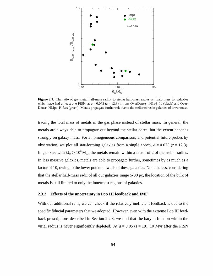
Figure 2.9 shows how far metals propagate in galaxies relative to the stellar cores. The
"gas metal half-mass radius" is calculated as the more familiar stellar half-mass radius, but
53
Figure 2.9. The ratio of gas metal half-mass radius to stellar half-massradius vs. halo mass for galaxieswhich have had at least one PISN, ata = 0.075 (z= 12.3) in runs OverDense_nH1e4_fid (black) and Over-Dense_HMpc_HiRes (green). Metals propagate further relative to the stellar cores in galaxies of lower mass.
tracing the total mass of metals in the gas phase instead of stellar mass. In general, the
metals are always able to propagate out beyond the stellar cores, but the extent depends
strongly on galaxy mass. For a homogeneous comparison, and potential future probes by
observation, we plot all star-forming galaxies from a single epoch,a = 0.075 (z = 12.3).
In galaxies withMh ≥ 108M⊙, the metals remain within a factor of 2 of the stellar radius.
In less massive galaxies, metals are able to propagate further, sometimes by as much as a
factor of 10, owing to the lower potential wells of these galaxies. Nonetheless, considering
that the stellar half-mass radii of all our galaxies range 5-30 pc, the location of the bulk of
metals is still limited to only the innermost regions of galaxies.
2.3.2 Effects of the uncertainty in Pop III feedback and IMF
With our additional runs, we can check if the relatively inefficient feedback is due to the
specific fiducial parameters that we adopted. However, even with the extreme Pop III feed-
back prescriptions described in Section 2.2.3, we find that the baryon fraction within the
virial radius is never significantly depleted. Ata = 0.05 (z = 19), 10 Myr after the PISN
54
explosion in the first star-forming galaxy, we findfb = 10.3% and 5.8% in runs Over-
Dense_ExtremeSN and OverDense_ExtremeRad, compared to 11.5% in the fiducial run.
In the case of the extremely energetic PISN, this is a relatively small resulting difference
for a 10-fold increase in the thermal energy and ionizing radiation output. The mass of the
galaxy at this epoch is 9×10⁶ M⊙, which we have shown to be large enough to withstand
standard Pop III feedback. On the other hand, the differenceis more pronounced in the
case of extreme ionizing feedback, indicating that the disruptive efficacy of supernovae is
significantly increased when it explodes in a region where neutral hydrogen has been more
effectively ionized and dispersed by radiative feedback.
The effect of both types of extreme feedback on the propagation of metals is stronger.
Metals tend to be blown out of galaxies anisotropically, often extending outwards in di-
rections orthogonal to filaments, into lower density regions. The galactocentric radius that
encloses 80% of the metals formed in the PISN stretches out to1.7Rvir 20 Myr after the
explosion in both run OverDense_ExtremeSN and run OverDense_ExtremeRad, compared
to just 0.91Rvir in the fiducial run. These metals do not fully escape the gravitational pull
of the galaxy, however, and 90 Myr after the explosion, the galaxies from both extreme
feedback runs contain 80% of the metals from the first PISN within the virial radius (in the
fiducial run, they are contained within just 0.15Rvir).
Though we increased the feedback effects by a factor of 10, only modest and temporary
differences were observed between the runs. Such inefficiency of feedback demonstrates
the weak coupling of thermal energy from PISNe to the ISM at the densities and tem-
peratures resolved by our simulations, as almost any amountof energy can be quickly
radiated away. This can be seen when considering typical cooling times in the ISM,
τcool = kbT/Λn ≈ 3000(T/104 K)(1 cm−3/n) yr, for Λ = 10−23 erg s−1 cm−3 (Hopkins et al.,
2011). The cooling time of the dense, filamentary gas surrounding the supernova remnant
(n = 10 cm−3, T = 104 K) is just ~300 yr, which is comparable to a typical timestep in our
simulations (~500 yr). This dense gas mixes with the shock-heated supernova remnant,
allowing the entire region to return to the ambient temperature of the ISM within a few
Myr.
The impact of extreme feedback is more pronounced in the IGM,particularly in run
55
OverDense_ExtremeRad. The mass fraction of ionized gas between 1-3 kpc from the
galactic center is enhanced by a factor of ~200, compared to the fiducial run, even 40
Myr after the PISN. Within the same distance range, the IGM temperature is a factor of
~10 higher at this epoch. The relatively hot and ionized IGM in turn could affect accretion
rates onto galaxies at later times.
The effect of making PISNe ten times more powerful in the H Mpcbox was more
drastic, as this box sampled lower mass galaxies. The baryonfraction in the first galaxy
dropped below 10−5 after the first PISN, compared to 1.7% in the standard run Over-
Dense_nH1e4_fid. The radii enclosing 80% of the baryons and metals are twice as large as
in the standard run, demonstrating that the added energy in this extreme run coupled with
the ISM more efficiently. Even with the standard feedback prescription we would expect a
strong blowout in a halo of this mass (2.7×10⁶M⊙ at this epoch). However, in the fiducial
run this galaxy ultimately gobbled up most of the ejected metals. On the other hand, the
extreme PISN energy (270×1051 erg) is able to completely destroy the high-density gas
clouds needed for star formation, prevent re-accumulationof dense gas from filaments, and
cause the metal ejecta to travel far enough into the IGM wherethey may never fall back
onto the galaxy.
These tests indicate that given enough energy input, the host halos of Pop III stars can
become completely devoid of gas for cosmologically-significant intervals of time, partic-
ularly when they are below the mass threshold ~3×10⁶M⊙. However, for the feedback
parameters currently considered realistic (our fiducial runs), the feedback of the first stars
is limited as illustrated in Figures 2.6 and 2.7.
In the run with low masses of Pop III stars (OverDense_LowMass), without any PISN,
metal transport is extremely ineffective. Ata = 0.055, 80% of the metals that have been
generated by stars in the first star-forming galaxy are confined within 75 pc of the galactic
center, compared to 420 pc in the fiducial run. This test demonstrates that if Pop III stars
did not have a top-heavy IMF, their contribution to enriching the IGM would be further
marginalized. These results agree qualitatively with the work of Ritter et al. (2012), who
argued that filamentary accretion was never significantly disrupted if Pop III stars had low
or moderate characteristic masses and exploded in type II supernovae.
56
2.4 Discussion and Conclusions
We have presented the results of simulations that implemented primordial star formation
in the cosmological code ART. We find that the effects of stellar feedback on the amount
of baryons and metals within the first galaxies depend strongly on galaxy mass. For the
lowest-mass galaxies (Mh ~106M⊙) our results are similar to those of Bromm et al. (2003);
Whalen et al. (2008); Wise & Abel (2008); Wise et al. (2012a), with gas and metals of-
ten being driven well beyond the virial radius of the Pop III star’s host galaxy. For more
massive galaxies (Mh ≥ 107M⊙), however, a single PISN is not effective in evacuating the
galactic ISM, as suggested by Wise & Cen (2009). Feedback fromPop III stars does not
typically inject enough energy into the massive halos to permanently photo-evaporate the
gas, and drive metal-rich outflows past the virial radius. While Pop III stars can temporar-
ily expel gas and quench star formation, the ISM begins to replenish soon after the SN
explosion, as accretion from filaments at this epoch is very fast. All galaxies considered in
our analysis with at leastMh ≈ 3×10⁶ M⊙, and some which are even less massive, appear
to have more than 50% of the universal baryon fraction restored 100 Myr after the first
Pop III supernova event. Metals are ejected anisotropically, and can travel relatively longer
distances through the diffuse IGM in directions perpendicular to the dense filaments which
feed galactic accretion. This means that it typically takesmore time for the ejected met-
als to be re-accreted into the galaxy, but we have demonstrated that this re-accretion does
frequently occur, even in low-mass galaxies.
The aforementioned dividing line ofMh ≈ 3× 10⁶M⊙ is important for determining
whether the energy injection from the supernova at the end ofthe star’s life can expel
gas and metals out to a significant distance. The concept of a dividing line between early
galaxies that suffer from significant blowout from those that do not has been considered in
prior work (e.g. Ciardi et al. 2000; Ricotti et al. 2002b). However, our results point to a
considerably lower threshold than what had been expected, as all but the very first galaxies
are apparently robust to PISN feedback when continued accretion from filaments and the
fallback of ejecta into the growing galaxy is considered. The strength of this conclusion
is bolstered by our use of a very strong feedback model for PopIII stars (even in our
57
fiducial runs). In addition, the first stars may have a lower characteristic mass (Greif et al.,
2011), which would make PISNe less frequent and the feedbackeffects would be further
marginalized (Ritter et al., 2012).
In order for simulations to capture the full range of relevant effects from Pop III star
formation, resolving halos around 106M⊙ with a sufficiently large number of particles is
critical. With insufficient resolution (less than 1000 DM particles for 106M⊙ halos), all
galaxies seem to reachM > 107M⊙ without having yet formed a star. Since these galaxies
are already beyond theMh ≈ 3×10⁶M⊙ dividing line, they display few disruptive effects
from Pop III feedback. Aggressive super-Lagrangian refinement may help resolve star for-
mation in halos of lower mass, but requires a prohibitively large number of computations.
A more practical approach is to begin simulations with sufficiently high resolution in the
initial conditions.
58
CHAPTER 3
The epoch of Population III stars
3.1 Introduction
The first stars in the universe formed in gas devoid of metals.This exotic environment may
have caused the initial mass function (IMF) for Population III stars to be different from the
modern day case. Namely, the high Jeans mass of metal-free gas suggests a top-heavy IMF
(Abel et al., 2000; Bromm et al., 1999; Abel et al., 2002; Yoshida et al., 2003). In turn,
the feedback processes in the first stars may have been more drastic, prompting the release
of extreme amounts of ionizing radiation (Tumlinson & Shull, 2000; Bromm et al., 2001a)
and the occurrence of pair instability supernovae (PISNe) (Heger & Woosley, 2002).
To explore the effects of these stars on their host galaxies,we developed a model for
Pop III star formation and feedback and implemented it into the adaptive refinement tree
(ART) code, as described in a companion paper, (Muratov et al. 2013a, see Chapter 2). Pop
III stars were modeled to form in gas that was dense, partially molecular, and of primordial
composition. Pop III SNe and ionizing radiation feedback were enhanced relative to their
Pop II counterparts, and the first PISNe seeded the ISM with metals. We ran a suite of
cosmological simulations with this model, and found that the dynamical impact of Pop III
feedback depended strongly on the galaxy mass. In agreementwith previous work in the
field (e.g. Bromm et al. 2003; Whalen et al. 2008; Wise et al. 2012a), we found that PISNe
were able to efficiently expel gas and metals from theMh ~106M⊙ halos expected to host
the very first stars (Tegmark et al., 1997). However, these effects were often temporary, as
cosmological inflows of fresh gas restored the baryon fraction to the universal value. The
metals, which had previously escaped past the virial radius, also typically fell back into the
growing potential wells of the accreting galaxies, leavingthe intergalactic medium (IGM)
59
mostly pristine. In galaxies with massMh > 107M⊙, most gas remained bound even after
a PISN event, and metals were not ejected past the virial radius.
Since Pop III stars by definition only form in primordial gas,the large amount of metals
released in PISNe leads to the ’self-termination’ of Pop IIIstar formation (Yoshida et al.,
2004). According to our findings in Chapter 2, this self-termination can only be local, as
enrichment of the IGM and external halos is rather minimal from single PISNe. Therefore,
determining the epoch when Pop III termination becomes universal is a somewhat different
question (Tornatore et al., 2007). Pop III star formation could be relevant for a much longer
phase of cosmic history if a Pop III star formed in every pristine halo withM & 106−108 M⊙
prior to reionization, as the abundance of such halos increases considerably with cosmic
time.
Population II star formation can commence in galaxies once they are either sufficiently
massive to enable the rapid gas cooling by atomic hydrogen lines, or enriched enough to
enable efficient metal cooling (Ostriker & Gnedin, 1996). Because the feedback of Pop
II stars is weaker than that of Pop III, Pop II star formation should ramp up rapidly in
the host galaxy, provided that accretion from filaments continues to bring new supply.
However, the relative weakness of the feedback, taken in conjunction with the plethora of
primordial sites where Pop III stars may still form, means that the host galaxy, as well
as the universe as a whole, are still influenced by Pop III stars for some time after Pop
II star formation begins. Though this scenario has already been explored through semi-
analytical models(e.g. Scannapieco et al. 2003; Yoshida etal. 2004; Schneider et al. 2006)
and numerical simulations (e.g. Tornatore et al. 2007; Maioet al. 2010, 2011; Greif et al.
2010; Johnson et al. 2013; Wise et al. 2012a), understandingthis transition quantitatively
is relevant for the ability of future observational facilities such as the James Webb Space
Telescope (JWST) to observe galaxies dominated by Pop III stars. Studies thus far have
shown that the first galaxies generally sit on the brink of detectability by JWST (Pawlik et
al., 2011, 2013; Zackrisson et al., 2011, 2012).
In this paper, we follow the evolution of the galaxies described in Chapter 2 through
the epoch of dominance of the first stars. This sample of simulated galaxies spans a range
of masses and accretion histories, therefore representinga broad variety of cosmic envi-
60
ronments. We study the transition from Pop III to Pop II star formation, and quantify the
duration of this epoch. We also explore the effect of cosmic variance, and determine the
prevalence and importance of Pop III stars at various cosmicepochs.
3.2 Simulations
A full description of our simulation setup, including the details of both the Pop III and Pop
II star formation recipes, is presented in Chapter 2. Here, weoutline the setup only briefly.
We perform the simulations with the Eulerian gasdynamics+N-body adaptive refinement
tree (ART) code (Kravtsov et al., 1997; Kravtsov, 1999, 2003; Rudd et al., 2008; Gnedin
& Kravtsov, 2011). We use a 2563 initial grid with up to 8 additional levels of refinement.
For most of our runs, we apply this grid to a 1h−1 Mpc comoving box with the WMAP-7
us a DM particle massmDM = 5.53×10³M⊙ and a minimum cell size of 22 comoving pc.
We also employ a 0.5h−1 Mpc comoving box, where using the same grid, the DM particle
mass is set tomDM = 690M⊙ and the minimal cell size is 11 comoving pc.
Pop III stars formed in the almost pristine gas with the abundance of heavy elements
below the critical metallicity log10Z/Z⊙ = −3.5 (Bromm et al., 2001b). Cells were allowed
to form Pop III stars if the gas density exceeded a thresholdnH,min, and a molecular hy-
drogen fraction thresholdfH2,min. Through a series of convergence tests, we found that
nH,min = 104 cm−3 and fH2,min = 10−3 were appropriate values for the two thresholds.
The Pop III prescription was designed to test the maximum possible effect of feedback,
relying on an IMF that was top-heavy. Half of the Pop III starsformed as 170M⊙ particles
and were set to explode in PISNe. Each PISN injected 27×1051 erg of thermal energy and
80M⊙ of metals into the ISM (Heger & Woosley, 2002). The remaining50% of Pop III
stars formed as 100M⊙ particles that explode in type II SNe, generating 2× 1051 erg of
energy. All Pop III stellar particles emited a factor of 10 more ionizing photons per second
than their Pop II counterparts of the same mass (Schaerer, 2002; Wise & Cen, 2009). A
suite of cosmological simulations performed with this model revealed that Pop III stars
drastically affected halos withMh < 3×10⁶ M⊙, but not halos of higher masses. Extended
convergence tests revealed that without sufficient mass resolution, it was easy to miss these
61
important dynamical effects.
In gas that is enriched beyond the critical metallicity, PopII star formation is modeled
according to the molecular-based star formation recipe presented in Gnedin et al. (2009)
and Gnedin & Kravtsov (2011).
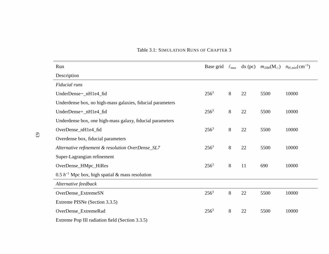
In Table 1 we list all of the simulations from the suite which we analyze in this paper.
Some of the simulations that were used in Chapter 2 for convergence tests and for determin-
ing the best parameters for Pop III star formation are not included here. In addition to the
three fiducial 1h−1 Mpc boxes (UnderDense−_nH1e4_fid, UnderDense+_nH1e4_fid, and
OverDense_nH1e4_fid), we study runs with extreme feedback,where we increased PISNe
energy (run OverDense_ExtremeSN) and ionizing photon emission (run OverDense_ExtremeRad)
by a factor of 10. We also include a run with a conservative "low-mass" Pop III IMF that
assigns the same feedback parameters to Pop III as for Pop II stellar particles (run Over-
Dense_LowMass) to account for the present uncertainty in the Pop III IMF (e.g. O’Shea &
Norman 2007; Greif et al. 2011).
In Chapter 2, we demonstrated that mass resolution was crucial for capturing Pop III
star formation in halos of massMh~106M⊙, and that halos withMh < 3× 10⁶M⊙ were
most susceptible to Pop III feedback. Our fiducial 1h−1 Mpc runs lacked the resolution
to study these objects effectively, but using the same grid on a smaller box increased the
resolution sufficiently while keeping the computational cost down. For this reason, we
also use a 0.5h−1 Mpc box (referred to as H Mpc) for run OverDense_HMpc_HiRes,to
test the validity of our results in the low-mass regime. Run OverDense_SL7 employs a
super-Lagrangian refinement, allowing for the simulation to more effectively zoom in on
overdense regions in primordial galaxies, allowing Pop IIIstars to form at early times in
low mass halos, hence extending the mass range of our sample.
62
Table 3.1: SIMULATION RUNS OFCHAPTER 3
Run Base grid ℓmax dx (pc) mDM(M⊙) nH,min(cm−3)
Description
Fiducial runs
UnderDense−_nH1e4_fid 2563 8 22 5500 10000
Underdense box, no high-mass galaxies, fiducial parameters
UnderDense+_nH1e4_fid 2563 8 22 5500 10000
Underdense box, one high-mass galaxy, fiducial parameters
OverDense_nH1e4_fid 2563 8 22 5500 10000
Overdense box, fiducial parameters
Alternative refinement & resolution OverDense_SL7 2563 8 22 5500 10000
Super-Lagrangian refinement
OverDense_HMpc_HiRes 2563 8 11 690 10000
0.5h−1 Mpc box, high spatial & mass resolution
Alternative feedback
OverDense_ExtremeSN 2563 8 22 5500 10000
Extreme PISNe (Section 3.3.5)
OverDense_ExtremeRad 2563 8 22 5500 10000
Extreme Pop III radiation field (Section 3.3.5)
63
OverDense_LowMass 2563 8 22 5500 10000
Pop III IMF and feedback mirror Pop II (Section 3.3.6)
Column 1.) Name of the run;
2.) Base grid, number of DM particles, number of root cells;
3.) Maximum number of additional levels of refinement;
4.) Minimum cell size at the highest level of refinement in comoving pc;
5.) DM particle mass in M⊙;
6.) Minimum H number density for Pop III star formation in cm−3;
7.) Further description of the run.
64
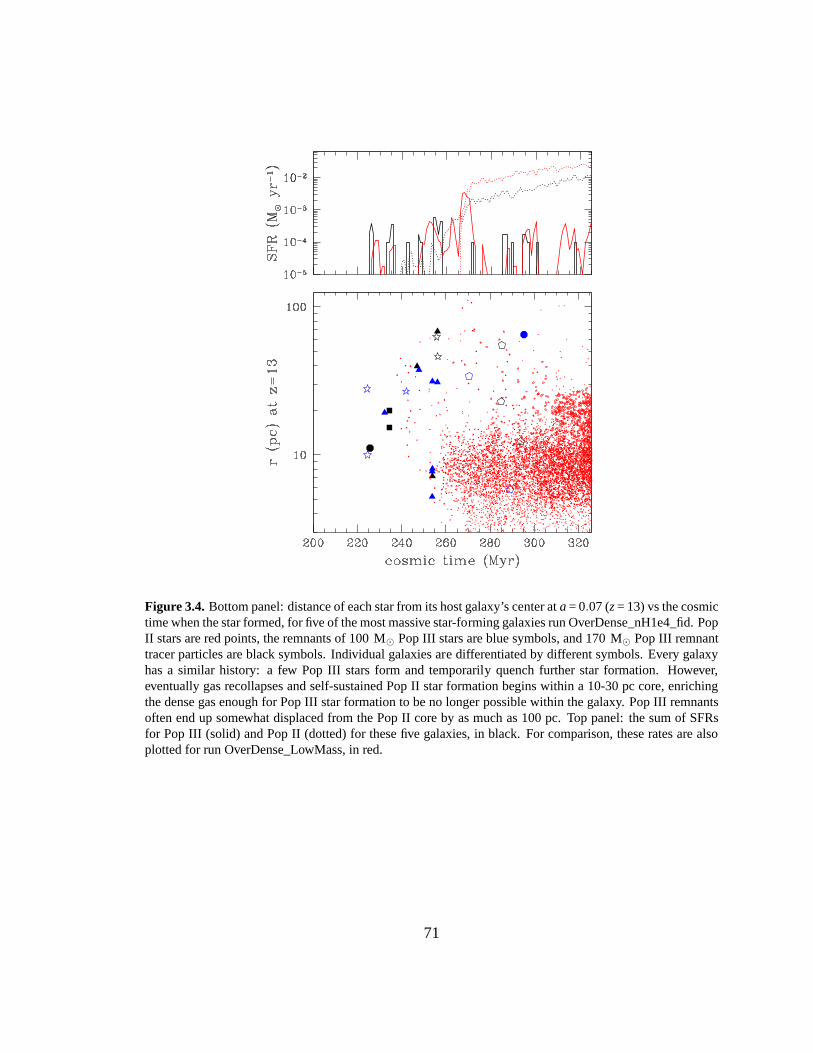
3.3 Results
3.3.1 Cosmic Variance
Using the DC mode formalism for the generation of initial conditions (Sirko, 2005; Gnedin
et al., 2011) allows us to test several representative regions of the universe without sacrific-
ing resolution, as would be needed were we to simulate a larger cosmological volume. With
a single parameter that stays constant over time in a given simulation box,∆DC, we encode
the amplitude of density fluctuations on the fundamental scale of the box. Although many
studies have been done to understand the effects of cosmic variance on the dark matter halo
mass function (Tinker et al., 2008), studying it in hydrodynamic simulations is significantly
more difficult. Here we present an analysis of the variance ofthe three different 1h−1 Mpc
boxes in our study. For reference, the DC mode values are∆DC = −2.57,−3.35, and 4.04 in
Box UnderDense−, UnderDense+, and OverDense respectively. The H Mpc box hasa DC
mode of∆DC = 5.04. Large positive values of∆DC indicate an overdense region.
The first Pop III stars form around scale factora≈ 0.047 (z≈ 20.3) in both Box Under-
Dense+ and Box OverDense. On the other hand, Box UnderDense− stalled significantly,
and no star formation occurs untila ≈ 0.073 (z≈ 12.7), translating to a time difference
of 165 Myr. This wide range demonstrates immediately that the epoch when Pop III star
formation begins is a strong function of local overdensity.If voids like the one represented
by Box UnderDense− are indeed not enriched by external sources, Pop III stars could have
existed in these voids until the end of cosmic reionization,at epochs that will be probed by
JWST (Hummel et al., 2012) and the Large Synoptic Survey Telescope (LSST) (Trenti et
al. 2009; but see Pan et al. 2012b).
Figure 3.1 shows the number of halos capable of hosting Pop III stars. Box Over-
Dense clearly dominates over the other two across the entiremass range, and since halo
mass strongly correlates with the density of central gas cells, Box OverDense is host to
many more star forming galaxies. Despite having fairly similar DC mode values, Box
UnderDense− and Box UnderDense+ have disparate halo abundances at the early epochs
considered in our study. This is particularly visible at thehigh-mass end, where the most
massive halo in Box UnderDense− has about 10 analogs in Box UnderDense+. The H Mpc
65
Figure 3.1. Cumulative number of halos vs. mass at two epochs for the three 1 h−1 Mpc boxes and one0.5 h−1 Mpc box. The smallest mass plotted corresponds to the earliest halo to form a Pop III star amongall of our runs. Box OverDense (black) has an order of magnitude more halos than Box UnderDense+ (red)and Box UnderDense− (blue) across almost the entire range of masses considered.While Box UnderDense+and Box UnderDense− have similar DC mode values, the former clearly has more massive halos. One BoxUnderDense+ galaxy in particular is on par with the most massive galaxies in Box OverDense. The H Mpcbox (green, run OverDense_HMpc_HiRes) represents only an eighth of the volume of the other boxes, andtherefore hosts fewer massive galaxies while still representing an overdense region.
box contains fewer halos than Box UnderDense+, but per unit volume it contains higher
density of massive halos, consistent with its higher∆DC value. At the time of formation of
the first stars (arounda= 0.05), none of the halos are more massive than 2×10⁷ M⊙. Figure
3.2 presents the star formation rate (SFR) density in each box for the runs with fiducial pa-
rameters. We can immediately see that SFRs vary by orders of magnitude among the three
boxes. Only two galaxies are able to form Pop III stars in the extreme void represented by
Box UnderDense−, and the total mass of Pop II is only 2300M⊙ by a = 0.1 (z= 9) in this
run. Such a narrow margin of error suggests that it is possible that with slightly different
parameters for the initial overdensity, galaxies in this box may have never been able to form
Pop III stars before all halos were stripped of gas by external ionizing radiation.
Box UnderDense+ and Box OverDense have similar global Pop IISFRs ata < 0.07
(z> 13), as each box is being dominated by only a few galaxies at early times. However,
66
Figure 3.2. The SFR density vs scale factor for runs UnderDense−_nH1e4_fid (blue squares), Under-Dense+_nH1e4_fid (red triangles), OverDense_nH1e4_fid (black circles), and OverDense_HMpc_HiRes(green pentagons). Global SFRs are significantly affected by the initial conditions in their respective simula-tion boxes. Pop III SFRs are denoted by open circles, Pop II SFRs by filled circles.
the disparity between the mean density of the boxes becomes evident at late times, as Box
OverDense becomes filled with a population of massive halos able to host dense cores
in which Pop III, and subsequently, Pop II star formation is initiated. Box UnderDense+
continues hosting only one such galaxy for a large fraction of the duration of the simula-
tion until a = 0.085, when an external halo of primordial composition reaches the Pop III
threshold density and later merges with the central galaxy.
In contrast to the large differences between the simulationboxes, we find the variance in
the SFR between various realizations within the same box to be low. Differences between
the setup of our test runs in Chapter 2 primarily affect Pop IIIstars, but ata = 0.055, the
total number of PopIII stars in Box OverDense was the same. Furthermore, Pop II stars
constitute most of the star formation ata > 0.07. Once a given galaxy transitions to Pop
II as the dominant stellar population, details of Pop III star formation do affect the history
of that galaxy. The Pop III SFR stays relatively constant between 10−5 and 10−4M⊙ yr−1
throughout the entire simulation. The range of values and relative constancy of this SFR up
to z~6 are similar to the results found in larger-scale (4 Mpc) SPH simulations by Johnson
67
et al. (2013).
The H Mpc box, represented here by run OverDense_HMpc_HiRes, samples a very
overdense region of the universe. The Pop III SFR density in this run significantly exceeds
the other boxes beforea = 0.065, but the Pop II SFR density never reaches the correspond-
ing values for Box OverDense and Box UnderDense+. This disparity results from the fact
that the 1 Mpc boxes ultimately sample more massive galaxieswhich are able to sustain
high Pop II star formation rates. Instead, a large fraction of low-mass galaxies simulated in
the H Mpc box have considerable gas blowout after PISNe, delaying Pop II star formation
for a cosmologically significant period of time.
3.3.2 The Ejection and Gobbling of Pop III Metals
The initial enrichment of the galactic ISM in our simulations happens almost exclusively
through internal Pop III SNe rather than external intergalactic winds. This means that
every galaxy will first have a phase during which Pop III starsconstitute the entirety of the
galactic stellar mass and drive all feedback. As our model considers only PISNe as a source
of metal feedback during this Pop III phase, the enrichment required to transition to Pop
II star formation is accomplished by at least one energetic PISN explosion. The explosion
can be particularly potent, as it occurs in a hot, ionized, and diffuse medium carved out by
the Pop III star’s enhanced ionizing radiative feedback. The explosion therefore disrupts,
or at least displaces, the dense gas necessary for further star formation.
We refer readers to Chapter 2, as well as prior work (e.g. Whalenet al. 2008) for a
detailed description of this process. Here, we note that theefficacy of the feedback of these
individual massive stars depends significantly on the galaxy mass at the time of Pop III
star formation. A ~106M⊙ "minihalo" can lose a significant fraction of its baryons, while
a more massive (~107M⊙) halo can better withstand the explosion. Most galaxies, partic-
ularly those in overdense environments, benefit from continued accretion from filaments,
and can re-accrete the lost metals and baryons even if they were initially ejected beyond
the virial radius. Particularly, many galaxies "gobble up" the metals that they previously
ejected through a combination of rapid growth of their virial radius and true gravitational
fallback of the ejecta. The virial radius of a given galaxy grows both because of continual
68
Figure 3.3. The timescale for a galaxy to re-accrete ("gobble up") 80% ofthe metals ejected by its PISN vs.halo mass at the time of the explosion. Open squares represent instances where the primary galaxy mergeswith a secondary that has already been enriched by internal star formation, preventing accurate tracing ofthe metals initially associated with the primary galaxy’s PISN. The more massive the galaxy, the shorter isthe gobble timescale. Plotted galaxies are from runs OverDense_nH1e4_fid, OverDense_SL7, and Over-Dense_HMpc_HiRes.
buildup of matter in the outer parts of galaxies, and becausethe virial radius depends on
the critical density of the universe, which evolves with redshift. In Figure 3.3, we show the
time it takes each galaxy to gobble up 80% of the mass of metalsgenerated in the initial
PISN. We confirm that this timescale is relatively rapid (50-100 Myr) for galaxies more
massive than the 3×10⁶ M⊙ threshold we discovered in Chapter 2. In galaxies which are
sufficiently massive (above ~107M⊙) at the time of the explosion, the metals rarely travel
further than the virial radius, hence the gobble timescale is short.
Galaxies below the 3×10⁶M⊙ threshold have longer gobble timescales, and occasion-
ally will merge with a more massive galaxy prior to the completion of the re-accretion
process. Such instances prevent accurate tracing of the metals associated with the original
PISN of the minihalo, and are therefore lower limits for the gobble timescales (denoted
by open squares in Figure 3.3). In particularly underdense environments with slow fila-
mentary accretion, the metals are permanently ejected fromthe minihalo. In run Over-
69
Dense_HMpc_HiRes, which resolves galaxies in the minihaloregime, only 20% of PISNe
result in such permanent ejections. The metals that are the result of the permanent ejections
do not pollute other halos sufficiently to initiate Pop II star formation over the course of
our simulations. Though these metals enrich the IGM, the total fraction of volume that is
enriched beyond the critical metallicity, log10Z/Z⊙ = −3.5, has a peak value of 0.05% at
z≈ 10.5 in our most minihalo-dominated simulation, run OverDense_HMpc_HiRes.
The scatter of the gobble timescale for galaxies of a given mass is largely associated
with their diverging mass accretion histories. We investigated the accretion history in both
absolute and relative terms. The absolute growth rate is computed as the change in halo
mass in the 100 Myr following the supernova. The relative growth is computed as the
timescale for the halo to double the virial mass it had at the time of the explosion. We
find that the absolute growth rate serves as a better predictor for the gobble timescale: all
galaxies withdM/dt > 0.2M⊙ yr−1 have a gobble timescale of less than 100 Myr, while
those with 0.04< dM/dt < 0.2M⊙ yr−1 show a wide range between 30 to 160 Myr. The
20% of PISNe that result in permanent ejections have growth rates under 0.04M⊙ yr−1 and
mass doubling timescales longer than 90 Myr (most longer than 150 Myr).
3.3.3 Transition to Normal Star Formation
For the remainder of the paper, we mainly deal with galaxies that are more massive than
3× 10⁶M⊙, and hence have relatively short gobble timescales. These galaxies typically
dominate the star formation rate in the simulation boxes at late times. In particular, in this
section, we focus on run OverDense_nH1e4_fid during the first140 Myr after the first star
forms. This corresponds to the range of scale factor 0.048< a < 0.07, or equivalently
20> z> 13. After that epoch the most massive galaxies in this box allform exclusively
Pop II stars. Even more importantly, bya = 0.07, all Pop III stars in these galaxies have
already exploded as SNe, and no longer provide radiative feedback. We will quantify the
duration of the Pop III epoch in Section 3.3.4.
70
Figure 3.4.Bottom panel: distance of each star from its host galaxy’s center ata= 0.07 (z= 13) vs the cosmictime when the star formed, for five of the most massive star-forming galaxies run OverDense_nH1e4_fid. PopII stars are red points, the remnants of 100 M⊙ Pop III stars are blue symbols, and 170 M⊙ Pop III remnanttracer particles are black symbols. Individual galaxies are differentiated by different symbols. Every galaxyhas a similar history: a few Pop III stars form and temporarily quench further star formation. However,eventually gas recollapses and self-sustained Pop II star formation begins within a 10-30 pc core, enrichingthe dense gas enough for Pop III star formation to be no longerpossible within the galaxy. Pop III remnantsoften end up somewhat displaced from the Pop II core by as muchas 100 pc. Top panel: the sum of SFRsfor Pop III (solid) and Pop II (dotted) for these five galaxies, in black. For comparison, these rates are alsoplotted for run OverDense_LowMass, in red.
71
Figure 3.4 shows the distance of each stellar particle from the center of its host galaxy
at a = 0.07 vs the cosmic time at which the stellar particle was formed. Five of the most
massive star-forming galaxies are stacked together in thisplot, showing the similarity in
the assembly history of these galaxies. We see that each of the five galaxies does not host
more than a few Pop III stars. If a 100M⊙ star is the first to form in a given galaxy, it
will not release any metals, and further Pop III star formation will be possible after the gas
recollapses. If on the other hand a 170M⊙ star is formed, Pop III star formation is rarely
possible in the same galaxy again. The metals generated by a single PISN from a 170M⊙
star are enough to switch the galaxy’s primary mode of star formation to be Pop II by
pushing the metallicity of gas above the critical thresholdlog10Z/Z⊙ = −3.5 (as has been
previously demonstrated e.g. Greif et al. 2010; Wise et al. 2012a). A few exceptions to this
pattern happen when the sites of Pop III star formation within the galaxy are sufficiently
spread apart (i.e. two Pop III stars form in two different halos that subsequently merge)
or alternatively, the Pop III stars form sufficiently close together in time. The latter case
is possible when many cells within the same giant molecular cloud reach the threshold
density for star formation and several Pop III stars form before their feedback disperses the
remaining gas in the cloud. This produces Pop III star multiples that are very close to each
other in location and age.
The spatial distributions of Pop III stellar remnants and Pop II stars within their host
galaxy are significantly different. Pop III stellar remnants can be found out to 70 pc from
the center, while most Pop II stellar particles at this epochare within 20 pc. Note that
the centers of the galaxies are defined to only ~5-15 pc, because of the limited number
of DM particles and force resolution. High-mass galaxies have better-defined centers than
low-mass galaxies. Both stellar populations generally form close to the center of the host
galaxy, but Pop III stars typically form at earlier times when the galaxy is not very massive,
and the spatial concentration of DM particles is not very high. In this environment, dense
star-forming gas has a clumpy structure, which is off-center from the DM cusp. After
powerful Pop III feedback ejects gas from this region, the Pop III remnants become less
bound, further increasing the apocenter of their orbit. On the other hand, Pop II stars are
rapidly produced only once the galaxy becomes relatively massive and concentrated, and
72
the DM center is more closely associated with the location ofthe densest gas. Pop II
thermal feedback and radiative feedback is not strong enough to shut off further Pop II star
formation near the galactic center, ultimately leading PopII stars to have a very high spatial
concentration.
3.3.4 Epoch of Equivalence
The duration of the Pop III epoch has been previously studied(e.g. Trenti & Stiavelli 2009)
by comparing the SFRs of the two populations, and finding the epoch where the Pop III SFR
drops off dramatically compared to Pop II. Our Figure 3.2 shows that bya = 0.07 (z= 13),
Pop II star formation is more common in all boxes except the void represented in Box
UnderDense−. However this approach may not properly account for the impact Pop III stars
have on the universe at early times, as Pop III stars are able to generate significantly more
thermal, ionizing, and metal feedback per baryon compared to their Pop II counterparts
(e.g. Tumlinson & Shull 2000). To more precisely quantify the impact of Pop III stars, we
compute the relative "budget" of thermal energy, metals, andionizing photons contributed
in each galaxy by the two stellar populations, integrated over the lifetimes of all stellar
particles. For the purpose of this analysis, we define the "epoch of equivalence" as the
time when Pop II stars have generated just as much ionizing radiation as their Pop III
counterparts. In turn, we define the "duration of the Pop III phase" as the length of time
from the formation of the first Pop III star to the epoch of equivalence.
A global picture of the feedback budget is shown in Figure 3.5. Here, we calculate
at each epoch the relative contribution of Pop III stars to the budget of ionizing photons,
thermal energy from SNe, and metals injected into the ISM in run OverDense_nH1e4_fid.
Every budget can be examined individually. Pop II stars haveproduced as many ionizing
photons as Pop III stars bya = 0.0633 (z= 14.8). The total thermal energy released by SNe
in Pop II stars surpasses that produced by Pop III stars ata = 0.0642 (z= 14.6). The total
mass of metals produced in Pop II stars surpasses that of Pop III at a = 0.0689 (z= 13.5).
Though we have chosen to define the epoch of equivalence in terms of ionizing radiation,
any one of these feedback quantities leads us to the conclusion that the duration of the Pop
III phase is short.
73
Figure 3.5. The fractional contribution of Pop III stars to the integrated feedback budget of the universe inrun OverDense_nH1e4_fid vs scale factor. This fraction is calculated separately for metals (blue), ionizingradiation (black), and thermal radiation due to SNe (red).
The exact timing of the epoch of equivalence can be affected by the simulation’s ability
to resolve low-mass halos that are susceptible to the deleterious effects of Pop III feedback,
and hence have longer delays for the onset of Pop II star formation. The resolution nec-
essary to probe such low-mass galaxies is not attained in runOverDense_nH1e4_fid. Run
OverDense_SL7 probes the same volume as run OverDense_nH1e4_fid, but Pop III stars
form at earlier times, when the host halos are less massive. In this run, the epochs of equiv-
alence shifts toa = 0.0633,a = 0.0674 and,a = 0.0710 for ionizing radiation, SNe thermal
energy, and metals, respectively. For run OverDense_HMpc_Hires, which resolves many
galaxies in the minihalo regime, the epoch of equivalence for the three types of feedback
is reached ata = 0.0721,a = 0.0735, anda = 0.0764. These consistently small shifts in the
duration of Pop III dominance give us no reason to believe that significant contributions of
feedback from Pop III stars are missed in simulations that fail to resolve minihalos.
We did not include Box UnderDense+ and UnderDense− in this analysis, as they sample
few star-forming galaxies and do not make significant contributions to the budget of either
Pop III or Pop II feedback.
74
To understand the transition to normal star formation in individual galaxies, we also
budget the feedback from stars within a given galaxy. All numbers quoted in this section
reflect the integrated total feedback contributions over the lifetime of stellar particles up
to the epoch considered. As a case study, we take the third galaxy to form a Pop III star
in run OverDense_nH1e4_fid. The first star forms ata = 0.055 (z = 17.2), when the halo
mass and gas mass of this galaxy are 9.8× 10⁶M⊙ and 1.2× 10⁶M⊙, respectively. At
a = 0.06 (z= 15.7, 23 Myr later) this galaxy has formed a total of 118M⊙ of Pop II stars.
The first and only Pop III star that formed in the galaxy was a 170M⊙ PISN progenitor.
Although the total mass of each stellar population is comparable, the one Pop III star still
has had dominant influence on the galaxy by way of its strongerfeedback. The Pop III
star contributed 98% of the metals, 88% of the ionizing photons, and 93% of the thermal
energy. This galaxy is clearly in the phase of its evolution where the effects of Pop III star
formation are most likely to be seen. However, we again note that despite this, the galaxy
has not been significantly perturbed by the Pop III star’s injection of energy. Only 1.7% of
its hydrogen is ionized, and all of the metals are confined in the gas well within the virial
radius.
By a = 0.0675 (80 Myr after the first star formed), one more Pop III starhas formed,
giving 270M⊙ of Pop III mass formed in the galaxy, but now the total Pop II mass has
increased to 1260M⊙. This second Pop III star has a metallicity of log10Z/Z⊙ = −4.7,
suggesting it formed in gas that was significantly enriched,but below the critical metallicity
of log10Z/Z⊙ = −3.5. Therefore, whether the star should be Pop III or Pop II is rather
sensitive to the particular setup of the model and stochastic effects. These two Pop III stars
still contribute 91% of the metals, 61% of the ionizing photons and 71% of the thermal
energy. We see that the energy contributions from Pop II stars are catching up with those of
Pop III stars, but the metal contribution of Pop III stars remains dominant. This confirms
the trend of Figure 3.5 that the large yield of metals produced by PISNe is the longest
lasting contribution of Pop III star formation.
By a = 0.075 (z= 12.3, 134 Myr after the first star formed), the epoch of Pop III stars
is clearly over in this galaxy despite the fact it has merged with another galaxy, which also
hosted a recent PISN progenitor Pop III star. The combined initial mass of Pop III stars is
75
Figure 3.6. The duration of the epoch of Pop III dominance vs halo mass of host galaxies ata = 0.1 (z =9). Plotted are galaxies in run OverDense_nH1e4_fid (black), run UnderDense+_nH1e4_fid (red), and runUnderDense−_nH1e4_fid (blue). More massive galaxies have shorter Pop III epochs.
now 440M⊙, while Pop II stars contribute 48000M⊙. The Pop III stars still contribute 26%
of the metal budget, but a mere 5% of the ionizing photon budget and 8% of the thermal
energy budget. Bya = 0.08, the Pop III metal contribution has finally dwindled away to
only 8%.
The epoch when Pop III stars have affected the evolution of the galaxy is thereby con-
fined to between the time when the first star formed (arounda≈ 0.055) and the time when
the budget of energy and metals of Pop II stars begins to dominate over Pop III stars
(a ≈ 0.07). The window of Pop III dominance only corresponds to∆a ≈ 0.015, or 100
Myr.
Figure 3.6 shows the duration of Pop III stars in this galaxy as well as in others, plotted
against halo mass ata= 0.1 (z= 9). We note that the length of the Pop III epoch is generally
between 20-200 Myr, confirming that the galaxy discussed in the above paragraphs is not
unique. The figure also reveals a trend where more massive galaxies exit the Pop III stage
earlier. These galaxies form in more biased regions, where the infall of fresh gas overcomes
the negative feedback generated by the thermal and ionizingradiation of Pop III stars, and
76
Figure 3.7. The epoch at which the contributions of Pop III and Pop II stars to the cumulative ionizingphoton budget are equal vs. halo mass of host galaxies ata = 0.1 (z= 9). Plotted are galaxies in run Over-Dense_nH1e4_fid (black), run UnderDense+_nH1e4_fid (red),and run UnderDense−_nH1e4_fid (blue). Theepoch of equivalence is earlier in more massive galaxies.
Pop II star formation erupts in the newly metal-enriched gas. Galaxies with higher mass at
the time of Pop III star formation can also radiate the PISN energy more efficiently.
Figure 3.7 shows that the epoch of equivalence for individual galaxies is also strongly
correlated with the mass of the halo ata= 0.1 (z= 9). This trend is perhaps not surprising, as
the sites of formation for the first stars have to be the most biased regions of the simulation
box, which would also produce the most massive galaxies. It is impressive, however, that
the trend is so definitive that it suggests we can predict the epoch at which Pop III stars
became subdued based simply on the halo mass.
We have also calculated the duration of the Pop III epoch by using the metal and ther-
mal energy budgets instead of the ionizing photon budget. The thermal energy dominance
of Pop III stars tends to last on average about ~10 Myr longer than the ionizing photon
epoch, with little variance, while Pop III metals remain dominant for ~20-50 Myr longer.
These differences are significant, and can be understood by looking at the relative effi-
ciency of metal production of 170M⊙ Pop III stars compared to Pop II counterparts. While
77
our Pop II stellar particles only generate an amount of metals equivalent to 1.1% of their
initial mass, 170M⊙ Pop III stars release almost 47% of their mass in metals following a
PISNe, meaning that Pop III metal feedback is ~40 times more effective. In comparison,
the number of ionizing photons per stellar baryon per lifetime is 6,600 for Pop II stars vs.
34,500 for 170M⊙ Pop III stars respectively, or only a factor of ~5 differencein efficiency.
The variation between individual galaxies can be caused by the number of non-enriching
100M⊙ Pop III stars that form there, and by the rate at which Pop II stars form, as their
feedback is released gradually over a longer interval of time. Despite this variation associ-
ated with using different feedback budget quantities, our conclusion on the brevity of the
Pop III epoch within each galaxy remains robust.
3.3.5 Extreme Pop III Feedback
The duration of the phase of Pop III dominance may depend on the details of the implemen-
tation of stellar feedback. Here, we consider two additional runs with artificially enhanced
Pop III feedback. Bya= 0.0625 (z= 15), the fiducial run OverDense_nH1e4_fid has 34 Pop
III stars, while run OverDense_ExtremeSN has 28 stars and the OverDense_ExtremeRad
run has 19 stars. At least part of this variation can be explained by the stochastic effect
that the OverDense_ExtremeRad run happened to form 170M⊙ PISNe progenitors more
frequently than the other runs, hence quenching further PopIII star formation in their
hosts. However, other evidence suggests that the extreme radiation does indeed quench
star formation very efficiently. This can be discerned by examining Pop II star forma-
tion, as 20000M⊙ formed in run OverDense_nH1e4_fid, 7000M⊙ formed in run Over-
Dense_ExtremeSN, and 4000M⊙ in run OverDense_ExtremeRad ata = 0.0625. While we
showed in Chapter 2 that the effects of baryon expulsion in individual galaxies are tempo-
rary in both extreme feedback runs as well as the fiducial run,the cumulative effect of many
more extreme feedback events appears to have suppressed of star formation at early times.
More specifically, the relatively high IGM temperature in run OverDense_ExtremeRad
(discussed in Chapter 2) means that newly accreted gas in thisrun will take longer to cool
and condense to the densities required for star formation. In our models, radiative feed-
back is more effective than SN thermal feedback as a means of regulating star formation
78
and modifying the structure of the ISM and IGM.
In both extreme feedback runs, the epoch of equivalence is pushed back relative to
the fiducial run, however it is always reached beforez = 13. The epoch of equivalence
for ionizing radiation increased byδa = 0.0073 in run OverDense_ExtremeRad, while
the epoch of equivalence for SN thermal energy increased byδa = 0.0068 in run Over-
Dense_ExtremeSN. Even the drastic modifications to Pop III feedback output causes only
marginal shifts in the duration of their epoch of dominance.
3.3.6 Low Mass Pop III IMF
Using a standard Miller & Scalo (1979) IMF for Pop III stars causes the duration of the
Pop III epoch to be somewhat shorter than in the top-heavy fiducial case. The epoch of
equivalence for ionizing radiation is reached in run OverDense_LowMass ata = 0.0622, a
mere 90 Myr after the first star forms.
However, the more important distinction in run OverDense_LowMass is the relative
lack of suppression of star formation within individual galaxies. Bya = 0.065 (z= 14.4),
the total stellar mass formed in run OverDense_LowMass is a factor of ~3 larger than in the
fiducial run OverDense_nH1e4_fid (see top panel of Figure 3.4). The majority of stellar
mass in both runs is contained in the three most massive star-forming galaxies, each of
which has more stellar mass in the run OverDense_LowMass. Inthis run, nearly all of
the stellar particles that formed in these three galaxies are within 10 pc of their galaxy’s
center, enriching the dense gas slowly and steadily to perpetuate further star formation. A
similar Pop II core is seen in the fiducial run, however some Pop II stars and Pop III stellar
remnants are found up to 100 pc from their galactic centers (see bottle panel of Figure 3.4).
3.4 Discussion and Conclusions
We find that Pop III star formation can be expected to extend until at leastz≈ 10. However,
Pop III stars are not the dominant source of any form of globalfeedback pasta ≈ 0.07
(z≈ 13) in our models, and only dominate individual galaxies for20 to 200 Myr.
The UV radiation of Pop III stars and their powerful supernovae can temporarily evac-
uate neutral gas from the first galaxies, creating an opportunity for ionizing flux from the
79
subsequent generations of Pop II stars to escape into the IGM. However, it is unlikely that
the escape fraction was high because, as we showed in Chapter 2, accretion from filaments
brings back most of the expelled gas on roughly the same timescale (~150 Myr) as the
duration of the Pop III phase. This means that by the time starformation resumes at the
center, the entire galaxy will again be surrounded by neutral gas, making it difficult for the
ionizing photons to escape.
We also showed in Chapter 2 that most of the metals generated inPISN would eventu-
ally fall back into the host galaxy rather than remaining in the IGM. This fact, combined
with the relative insignificance of the Pop III metal budget,leads us to conclude that Pop
III stars did not play much of a role in enriching the IGM, and that instead enrichment hap-
pened by normal stellar populations during and after the epoch of reionization. Though Pop
III star formation is self-limiting in individual galaxies, the absence of universal enrichment
implies that Pop III stars could form in underdense regions long after the universe has pri-
marily transitioned to normal star formation. It is in the least massive galaxies that formed
in underdense regions where we might expect to find the most recent signatures of Pop
III stars, suggesting that ultra-faint dwarf spheroidal galaxies and their disrupted remnants
within the Milky Way stellar halo may be the best place to look. As the chemical signature
of PISNe metals is expected to be different from that of Type II SNe, and the metal budget
of Pop III stars is the last feedback tracer to be overtaken byPop II, studying the spectra of
old metal-poor stars with peculiar chemical abundances maybe one of the most promising
ways to observationally constrain the chemical history of the first galaxies. The first efforts
in this field of ’stellar archeology’ have already yielded interesting results (e.g. Frebel et
al. 2007; Frebel & Bromm 2012), but there is more work to be done to increase the sample
of metal-poor stars, and to improve our knowledge of their abundances, many of which
are currently too faint for detailed spectroscopy. The nextgeneration of spectroscopic and
photometric surveys, such as Gaia-ESO and SkyMapper, will significantly improve the
sample, while the light collecting area of upcoming large ground-based optical telescopes
will enable detailed follow-ups of significantly fainter candidates (Frebel, 2011).
According to mock observational analysis for JWST by Pawlik et al. (2013), galaxies
with SFR in excess of 0.1M⊙ yr−1 may be detectable atz > 10. Only two galaxies in
80
our simulation box meet this criterion in the final snapshot at z= 9, and both are evolved
far beyond the point where Pop III stars made a significant contribution to their feedback
budgets. According to a separate analysis by Zackrisson et al. (2012), JWST surveys that
target gravitationally lensed fields are much more likely todiscover primordial galaxies
than ultra-deep unlensed fields. These authors suggest thatgalaxies in which 0.1% of
baryons are in the form of Pop III stars are detectable through direct starlight if they are in
the lensed field of the galaxy cluster J0717.5+3745. However, none of our galaxies meet
this criterion at any given time.
A more promising way to detect galaxies that are still dominated by Pop III stars is by
looking for PISN events directly. The light curve of a PISN isthought to have a similar
peak luminosity to SN Ia, but can remain bright for hundreds of days, producing a distinct
signature (e.g. Scannapieco et al. 2005). This idea has beenexplored and shown to be
feasible for both LSST (Trenti et al., 2009) and JWST (Hummel et al., 2012; Pan et al.,
2012a; Whalen et al., 2012). Again, considering our findings that underdense regions of
the universe may remain pristine until late times, we conclude that the best approach for
observing campaigns is to focus on areas where the spatial clustering signal is low, such
as cosmic filaments that connect two bright galaxies, to maximize the number of bright,
low-redshift detections.
If Pop III stars instead formed with a normal IMF (e.g. Greif et al. 2011), they would
have even less impact on the universe, as demonstrated by ourlow-mass IMF run. On
the other hand, while our extreme feedback runs showed that the Pop II transition could
be delayed with stronger Pop III feedback parameters, the transition inevitably happened
beforez = 13 and takes less than 250 Myr for even the least massive galaxies. In both
cases, our modifications to the feedback output were simplistic ways to test the range of
potential impact of Pop III stars without detailed modelingof additional physical processes.
However, it is becoming clear that missing physics in galaxyformation simulations can
have a wide variety of effects that are not accounted by our limited approach. For example,
momentum-driven winds from radiation pressure can significantly stir the ISM increasing
its susceptibility to other forms of feedback (Wise et al., 2012b; Agertz et al., 2013). The
presence or absence of dust can affect the shielding capabilities of molecular clouds from
81
UV radiation, thereby modifying fragmentation and potentially the IMF of stars (Aykutalp
& Spaans, 2011). Dark matter annihilation (Smith et al., 2012), cosmic rays (Jasche et
al., 2007; Stacy & Bromm, 2007; Uhlig et al., 2012), magneticfields (Turk et al., 2012),
and X-ray feedback from the first black holes (Haiman, 2011; Jeon et al., 2012) could
also be potentially important. We plan to explore them further in the next generation of
simulations.
82
CHAPTER 4
Modeling the Metallicity Distribution of Globular Clusters
4.1 Introduction
A self-consistent description of the formation of globularclusters remains a challenge to
theorists. A particularly puzzling observation is the apparent bimodality, or even multi-
modality, of the color distribution of globular cluster systems in galaxies ranging from
dwarf disks to giant ellipticals (reviewed by Brodie & Strader, 2006). This color bimodal-
ity likely translates into a bimodal distribution of the abundances of heavy elements such
as iron. We know this to be the case in the Galaxy as well as in M31, where relatively
accurate spectral measurements exist for a large fraction of the clusters. In this paper we
will interchangeably refer to metal-poor clusters as blue clusters, and to metal-rich clusters
as red clusters.
Bimodality in the globular cluster metallicity distribution of luminous elliptical galax-
ies was proposed by Zepf & Ashman (1993), following a theoretical model of Ashman &
Zepf (1992). The concept of cluster bimodality became universally accepted because the
two populations also differ in other observed characteristics. The system of red clusters
has a significant rotation velocity similar to the disk starswhereas blue clusters have little
rotational support, in the three disk galaxies observed in detail: Milky Way, M31, and M33
(Zinn, 1985). In elliptical galaxies, blue clusters have a higher velocity dispersion than red
clusters, both due to lack of rotation and more extended spatial distribution. Red clusters
are usually more spatially concentrated than blue clusters(Brodie & Strader, 2006). All
of these differences, however, are in external properties (location and kinematics), which
reflectwherethe clusters formed, but nothow. The internal properties of the red and blue
clusters are similar: masses, sizes, and ages, with only slight differences. Even the metal-
83
licities themselves differ typically by a factor of 10 between the two modes, not enough
to affect the dynamics of molecular clouds from which these clusters formed. Could it be
then that both red and blue clusters form in a similar way on small scales, such as in giant
molecular clouds, while the differences in their metallicity and spatial distribution reflect
when and where such clouds assemble?
All scenarios proposed in the literature assumed differentformation mechanisms for
the red and blue clusters, and most scenarios envisioned thestellar population of one mode
to be tightly linked to that of the host galaxy (e.g., Forbes et al., 1997; Cote et al., 1998;
Strader et al., 2005; Griffen et al., 2010). The other mode isassumed to have formed dif-
ferently, in some unspecified “primordial” way. This assumption only pushed the problem
back in time but it did not solve it. For example, Beasley et al. (2002) used a semi-analytical
model of galaxy formation to study bimodality in luminous elliptical galaxies and needed
two separate prescriptions for the blue and red clusters. Intheir model, red clusters formed
in gas-rich mergers with a fixed efficiency of 0.007 relative to field stars, while blue clusters
formed in quiescent disks with a different efficiency of 0.002. The formation of blue clus-
ters also had to be artificially truncated atz= 5. Strader et al. (2005), Rhode et al. (2005),
and Griffen et al. (2010) suggested that the blue clusters could instead have formed in very
small halos atz> 10, before cosmic reionization removed cold gas from such halos. This
scenario requires high efficiency of cluster formation in the small halos and also places
stringent constraints on the age spread of blue clusters to be less than 0.5 Gyr. Unfortu-
nately, even the most recent measurements of relative cluster ages in the Galaxy (De Angeli
et al., 2005; Marín-Franch et al., 2009; Dotter et al., 2010)cannot detect age differences
smaller than 9%, or about 1 Gyr, and therefore cannot supportor falsify the reionization
scenario. Dotter et al. (2010) also show that the red clusters have larger dispersion of ages
(15%, or about 2 Gyr) and those located outside 15 kpc of the Galactic center tend to show
measurably lower ages, by as much as 50% (or 6 Gyr). In addition, Strader et al. (2009)
find that the red clusters in M31 have lower mass-to-light ratios than the blue clusters,
possibly indicating an age variation.
In this paper we set out to test whether a common mechanism could explain the for-
mation of both modes and produce an entire metallicity distribution consistent with the
84
observations. We begin with a premise of the hierarchical galaxy formation in aΛCDM
universe. Hubble Space Telescope observations have convincingly demonstrated one of the
likely formation routes for massive star clusters today – inthe mergers of gas-rich galaxies
(e.g., Holtzman et al., 1992; O’Connell et al., 1995; Whitmoreet al., 1999; Zepf et al.,
1999). We adopt this single formation mechanism for our model and assume that clusters
form only during massive gas-rich mergers. We follow the merging process of progenitor
galaxies in a Galaxy-sized environment using a set of cosmological N-body simulations.
We need to specify what type and how many clusters will form ineach merger event. For
this purpose, we use observed scaling relations to assign each dark matter halo a certain
amount of cold gas that will be available for star formation throughout cosmic time and an
average metallicity of that gas. In order to keep the model transparent, we choose as simple
a parametrization of the cold gas mass as possible. Finally,we make the simplest assump-
tion that the mass of all globular clusters formed in the merger is linearly proportional to
the mass of this cold gas.
Although such model appears extremely simplistic, we have some confidence that it
may capture main elements of the formation of massive clusters. Kravtsov & Gnedin
(2005) used a cosmological hydrodynamic simulation of the Galactic environment at high
redshiftsz> 3 and found dense, massive gas clouds within the protogalactic disks. If the
high-density regions of these clouds formed star clusters,the resulting distributions of clus-
ter mass, size, and metallicity are consistent with those ofthe Galactic metal-poor clusters.
In that model the total mass of clusters formed in each disk was roughly proportional to the
available gas mass,MGC ∝ Mg, just as we assume here.
We tune the parameters of our semi-analytical model to reproduce the metallicity dis-
tribution of the Galactic globular clusters, as compiled byHarris (1996). This distribution
is dominated by the metal-poor clusters but is also significantly bimodal. We attempt to
construct a model without explicitly differentiating the two modes and test if bimodality
could arise naturally in the hierarchical framework.
We adopt a working definition of red clusters as having [Fe/H] > −1 and blue clusters
as having [Fe/H] < −1. This definition should also roughly apply to extragalactic globular
cluster systems. We use the concordance cosmology withΩ0 = 0.3, ΩΛ = 0.7, h = 0.7.
85
4.2 Prescription for Globular Cluster Formation
4.2.1 Cold Gas Fraction
We follow the merging process of protogalactic dark matter halos using cosmologicalN-
body simulations of three Milky Way-sized systems described in Kravtsov et al. (2004).
The simulations were run with the Adaptive Refinement Tree code (Kravtsov et al., 1997)
in a 25h−1 Mpc box. Specifically, we use merger trees for three large host halos and their
corresponding subhalo populations. The three host halos contain∼ 106 dark matter parti-
cles and have virial masses∼ 1012M⊙ atz= 0. Two halos are neighbors, located at 600 kpc
from each other. The configuration of this pair resembles that of the Local Group. The third
halo is isolated and is located 2 Mpc away from the pair. All three systems experience no
major mergers atz< 1 and thus could host a disk galaxy like the Milky Way.
In addition to the host halos, the simulation volume contains a large number of dwarf
halos that begin as isolated systems and then at some point accrete onto the host halo. Some
of these satellites survive as self-gravitating systems until the present, while the rest are
completely disrupted by the tidal forces. We allow both the host and the satellite systems
to form globular clusters in our model.
We adopt a simple hypothesis, motivated by the hydrodynamicsimulation of Kravtsov
& Gnedin (2005), that the mass in globular clusters,MGC, that forms in a given protogalac-
tic system is directly proportional to the mass of cold gas inthe system,Mg. We define the
corresponding mass fraction,fg, of cold gas that will be available for star cluster formation
in a halo of massMh as
fg ≡Mg
fb Mh, (4.1)
where fb ≈ 0.17 is the universal baryon fraction (Komatsu et al., 2011).
The gas fraction cannot exceed the total fraction of baryonsaccreted onto the halo,
which is limited by external photoheating and depends on thecutoff massMc(z):
fin =1
(1+ Mc(z)/Mh)3. (4.2)
We use an updated version of the cutoff mass as a function of redshift (originally defined
86
by Gnedin 2000), based on our fitting of the results of recent simulations by Hoeft et al.
(2006), Crain et al. (2007), Tassis et al. (2008), and Okamotoet al. (2008):
Mc(z) ≈ 3.6×10⁹ e−0.6(1+z) h−1M⊙. (4.3)
Given the scatter in simulation results and the numerical limitations of the modeling of gas
physics, a reasonable uncertainty in this mass estimate is of the order 50%. However, the
resulting cluster mass and metallicity distributions are not very sensitive to the exact form
of this equation. Note that Orban et al. (2008) provided an earlier revision of the equation
for Mc(z); our current form is more accurate. IfMc(z) falls below the mass of a halo with
the virial temperature of 104 K, we setMc(z) equal to that mass:
Mc,min(z) = M4 ≡ 1.5×10¹⁰∆
−1/2vir
H0
H(z)h−1M⊙, (4.4)
where∆vir = 180 is the virial overdensity andH(z) is the Hubble parameter at redshiftz.
This criterion ensures that we only select halos able to coolefficiently via atomic hydrogen
recombination lines.
Some of the baryons accreted onto a halo may be in a warm or hot phase (atT > 104 K)
unavailable for star formation, thusfg < fin < 1. We assume that only the gas in cold phase
(T ≪ 104 K) is likely to be responsible for star cluster formation. The cold gas fractionfg is
calculated by combining several observed scaling relations. From the results of McGaugh
(2005), the average gas-to-stellar mass ratio in nearby spiral and dwarf galaxies can be
fitted asMg
M∗
≈(
M∗
Ms(z)
)−0.7
, (4.5)
whereMs is a characteristic scale mass, which we found to beMs(z= 0)≈ 4×10⁹M⊙. This
relation saturates at low stellar masses, wherefg cannot exceedfin. At higher redshift the
only information on the gas content of galaxies comes from the study by Erb et al. (2006)
of Lyman break galaxies atz= 2. These authors estimated the cold gas mass by inverting
the Kennicutt-Schmidt law and using the observed star formation rates. These estimates are
fairly uncertain and model-dependent. Within the uncertainties, their results can be fitted
87
by the same formula but with a different scale mass:Ms(z= 2)≈ 2×10¹⁰M⊙. To extend
this relation to all epochs, we employ a relation that interpolates the two values:
Ms(z) ≈ 109.6+0.35z M⊙. (4.6)
An additional scaling relation is needed to complement equation (4.5) with a prescrip-
tion for stellar mass as a function of halo mass. We compile itby combining the ob-
served stellar mass–circular velocity correlation with the theoretical circular velocity–halo
mass correlation. Woo et al. (2008) found that the stellar mass of the dwarf galaxies in
the Local Group correlates with their circular velocities,which are taken as the rotation
velocity for the irregular galaxies or the appropriately scaled velocity dispersion for the
spheroidal galaxies. In the range 107M⊙ < M∗ < 1010M⊙, appropriate for the systems that
may harbor globular clusters, the correlation isVc ∝ M0.27±0.01∗ . This can be inverted as
M∗ ≈ 1.6×10⁹ M⊙ (Vc/100 km s−1)3.7.
CosmologicalN-body simulations show that dark matter halos, both isolated halos
and satellites of larger halos, exhibit a robust correlation between their mass and max-
imum circular velocity (e.g., Fig. 6 of Kravtsov et al., 2004): Vmax ≈ 100 (Mh/1.2×
1011M⊙)0.3 km s−1. This maximum circular velocity of dark matter is typicallylower than
the rotation velocity of galaxies because of the contribution of stars and gas. To connect
the two velocities, we apply the correctionVc =√
2Vmax, which reflects the observation that
the mass in dark matter is approximately equal to the mass in stars over the portions of
galaxies that contain the majority of stars. Then the equations in the last two paragraphs
lead toM∗ ≈ 5.5×10¹⁰(Mh/1012M⊙)1.1 M⊙.
We also need to extend this local relation to other redshifts. Conroy & Wechsler (2009)
matched the observed number densities of galaxies of given stellar mass with the predicted
number densities of halos of given mass fromz = 0 to z∼ 2, averaged over the whole
observable universe. They find that the stellar fractionf∗ peaks at massesMh ∼ 1012M⊙
and declines both at lower and higher halo masses. The range of masses of interest to us
is below the peak, where we can approximatef∗ dependence on halo mass as a power-law.
The results from Fig. 2 of Conroy & Wechsler (2009) are best fit by a steeper relation
88
than we derived for the Local Group and also show significant variation with redshift at
lower halo masses∼ 1011M⊙: M∗ ∝ M1.5h (1+ z)−2 (there is much less variation with time
around the peak at 1012M⊙, implying only a weak evolution in the total stellar density
at z < 1). We adopt the same redshift dependence to our local relation, while using the
shallower slope derived from Woo et al. (2008) because it deals with a population of halos
in the mass range corresponding to the Milky Way progenitors. The stellar mass fraction
of isolated halos is thus
f∗ =M∗
fbMh≈ 0.32
(
Mh
1012M⊙
)0.1
(1+ z)−2. (4.7)
This relation steepens at low masses because of two additional limits on the gas and stellar
fractions, which we impose to constrain the range of equations (4.5–4.7) to be physical.
First, the sum of the gas and stars (“cold baryons”) cannot exceed the total amount of
accreted baryons in a halo:
f∗ + fg ≤ fin. (4.8)
At each redshift, there is a transition massMh,cold, below which f∗ + fg = fin and above
which f∗ + fg < fin. For massesM < Mh,cold (but not too low, see next paragraph), we set
fg,revised= fin − f∗, with f∗ still given by equation (4.7). We consider the baryons that are not
included in fg or f∗ to be in the warm-hot diffuse phase of the interstellar medium.
Second, the ratio of stars to cold baryons,µ∗ ≡ f∗/( f∗ + fg), is not allowed to increase
with decreasing halo mass. For massive halos (Mh > Mh,cold) µ∗ monotonically decreases
with decreasing mass because of the condition (4.5). At someintermediate massesMh,µ <
Mh < Mh,cold, µ∗ continues to decrease but the gas fraction is reduced by the condition (4.8).
At Mh < Mh,µ, µ∗ would reverse this trend and increase with decreasing halo mass because
the cold gas is almost completely depleted. Such a reversal is unlikely to happen in real
galaxies, which would not be able to convert most of their cold gas into stars. Therefore,
for all massesMh < Mh,µ we fix µ∗ to be equal to the minimum value reached atMh,µ. This
affects bothf∗ and fg.
We expect our stellar mass prescription to apply in the rangeof halo masses from 109 to
1012M⊙, at least for the Local Group. However, this relation breakswhen a halo becomes a
89
Figure 4.1.Gas mass fraction (solid lines) and stellar mass fraction (dotted lines) vs. halo mass in our modelat redshiftsz= 0,1,2,3,4,5,6. Stellar fractions monotonically increase with time while gas fractions decreasewith time. The kink in the curves is due to our restriction on the maximum stellar fraction via eq. (4.8).
satellite of a larger system. Satellite halos often have dark matter in the outer parts stripped
by tidal forces of the host, while the stars remain intact in the inner parts. Unless the
satellite is completely disrupted, we keep its stellar massfixed at the value it had at the
time of accretion, even though the halo mass may subsequently decrease.
The simultaneous effects of the above scaling relations aredifficult to understand as
equations. Figure 4.1 illustrates graphically the values of the gas and stellar fractions
used in our model at various cosmic times. Atz= 0 the gas fraction peaks for halos with
Mh ∼ 3× 10¹⁰ M⊙. At lower masses it is reduced by the amount of accreted baryons
(eq. 4.8), while at higher masses it is reduced by the gas-to-stars ratio (eq. 4.5). The
stellar fraction follows equation (4.7) at high masses but drops faster at low masses be-
cause of the constraint (4.8). For a Galaxy-mass halo,Mh ≈ 1012M⊙, our model gives
M∗ ≈ 5.5× 10¹⁰M⊙ andMg ≈ 9× 10⁹M⊙. These numbers are consistent with the ob-
served amount of the disk and bulge stars and the atomic and molecular gas in the Galaxy,
from Binney & Tremaine (2008).
At earlier epochs at all masses of interest, the gas fractionis higher and the stellar
90
Figure 4.2. Same as Fig. 4.1, but for an alternative stellar mass prescription, eq. (4.9).
fraction is lower. There is a range of halos withMh & 1010 M⊙, which have an almost 100%
gas fraction at redshiftsz> 3. Such halos should be most efficient at forming massive star
clusters.
We realize that our adopted relations for the evolution of the stellar and gas mass are
not unique, as we are basing each fit on two data points. In order to test the sensitivity of
our results to these assumptions, we consider alternative functional forms for these fits in
Section 4.4.5. In particular, we give the stellar fraction asteeper dependence on halo mass
and weaker dependence on cosmic time:
f∗,alt = 0.32
(
Mh
1012M⊙
)0.5
(1+ z)−1. (4.9)
Such a slower evolution of the stellar mass is consistent with the observational studies of
Borch et al. (2006), Bell et al. (2007), and Dahlen et al. (2007). The corresponding gas and
stellar fractions are shown in Figure 4.2. Note that the amount of cold gas available for
cluster formation is not strongly affected by this change (compare Figs. 4.1 and 4.2).
91
4.2.2 Rate of Cluster Formation
Having fixed the parametrization of the available cold gas, we then relate the gas mass of a
protogalaxy to the combined mass of all globular clusters itcan form within∼ 108 yr (the
timescale of the simulation output). We based it on the rate derived in Kravtsov & Gnedin
(2005):
MGC = 3×10⁶ M⊙ (1+ p2)Mg/ fb
1011M⊙
. (4.10)
An additional factor, 1+ p2, allows us to boost the rate of cluster formation. Such a boost
may be needed because we form new clusters only at arbitrarily chosen epochs correspond-
ing to the simulation outputs. Unresolved mergers between the outputs may requirep2 > 0.
In our model we find the best fit to the Galactic metallicity distribution for p2 ∼ 3 (see Ta-
ble 4.1).
Note also that equation (4.10) imposes the minimum mass of a halo capable of forming
a globular cluster. Based on dynamical disruption arguments (Section 4.3) we track only
clusters more massive thanMmin = 105M⊙. Since we always haveMg < fb Mh, in order to
form even a single cluster with the minimum mass, the halo needs to be more massive than
109M⊙. For gas-rich systems at high redshift,MGC ∼ 10−4Mg/ fb ∼ 10−4 Mh.
Given the combined mass of all clusters to be formed in an event, MGC, our procedure
for assigning masses to individual clusters is as follows. We first draw the most massive
cluster, which we call the nuclear star cluster, even thoughwe do not have or use the
information about its actual location within the host galaxy and it is not important for our
current study. The mass assigned to the nuclear cluster,Mmax, is derived from the assumed
initial cluster mass function,dN/dM = M0M−2:
1 =∫ ∞
Mmax
dNdM
dM, (4.11)
which givesMmax = M0. This normalization is constrained by the integral clustermass:
MGC =∫ Mmax
Mmin
MdNdM
dM = MmaxlnMmax
Mmin. (4.12)
The power-law initial mass function agrees both with the observations of young star clus-
92
ters and the hydrodynamic simulations. After the nuclear cluster is drawn, the masses of
smaller clusters are selected by drawing a random number 0< r < 1 and inverting the
cumulative distribution:r = N(< M)/N(< Mmax):
M =Mmin
1− r(
1− Mmin/Mmax) . (4.13)
We continue generating clusters until the sum of their masses reachesMGC.
The formation of clusters is triggered by a gas-rich major merger of galaxies, which
includes mergers of satellite halos onto the main halo as well as satellite-satellite mergers.
New clusters form when the halo mass ati-th simulation output exceeds the mass at the
previous output by a certain factor, and at the same time the cold gas fraction exceeds a
Also, we require that the maximum circular velocity does notdecrease in this time step, to
ensure that the mass increase was real rather than a problem with halo identification. We
have experimented with a more relaxed criterion for the mainhalo than for satellite halos,
with p3,main < p3,sat, but did not find a significantly better fit to the mass or metallicity
distributions. We therefore keep a single value ofp3 for all halos.
For some model realizations, we consider an optional alternative channel for cluster
formation without a detected merger, if the cold gas fraction is very high:
case−2 : fg > p5, (4.15)
where the thresholdp5 is expected to be close to 100%. This channel allows continuous
cluster formation at high redshift when the galaxies are extremely gas-rich. High-redshift
galaxies are probably in a continuous state of major and minor merging, but because of
their lower masses it is more difficult to detect such mergersin the simulation. Additional
motivation for this channel follows from some nearby starburst galaxies that are forming
young massive clusters despite appearing isolated.Case-2 formation is allowed only for
93
Table 4.1.FIDUCIAL MODEL PARAMETERS
Parameter Value Effectσmet 0.1 log-normal dispersion of mass-metallicity relationp2 3.0 boost of the rate of cluster formationp3 0.2 minimum merger ratiop4 0.04 minimum cold gas fraction forcase-1 formationp5 0.98 minimum cold gas fraction forcase-2 formation
isolated halos before they are accreted into larger systemsand become satellites. The epoch
of accretion is defined by the last timestep before the orbit of the subhalo falls permanently
within the virial radius of its host.
Our model sample combines clusters formed in the main halo and in its satellites, either
surviving or disrupted. We exclude clusters from the satellites that have a galactocentric
distance atz= 0 greater than 150 kpc, which is the largest distance of a Galactic globular
cluster. We apply the criteria for cluster formation at every timestep of the simulation
(every∼ 108 yr) for each of the three main halos and their satellite populations. The rate
of cluster formation per every merger event is therefore approximatelyMGC/108 yr.
In order to compare the distribution of clusters obtained from our analysis to the dis-
tribution of Galactic globular clusters, we normalize the total number of model clusters by
the ratio of the Galaxy mass to the simulated halo masses atz= 0:
Nnormalized= NmodelMMW
Mh1 + Mh2 + Mh3. (4.16)
We takeMMW = 1012M⊙ and useMh1 = 2.37×10¹²M⊙, Mh2 = 1.77×10¹²M⊙, andMh3 =
1.70×10¹²M⊙ from Kravtsov et al. (2004).
4.2.3 Metallicity
The iron abundance is assigned to each model cluster according to the estimated average
metallicity of its host galaxy. The latter we obtain from themass-metallicity relation for
dwarf galaxies of the Local Group atz= 0 as formulated by Woo et al. (2008):
[Fe/H]0 = −1.8+ 0.4log
(
M∗
106M⊙
)
. (4.17)
94
In fact, the same fit is valid for the smallest, ultrafaint dwarfs studied by Kirby et al. (2008).
Thus we apply this relation to all protogalactic systems in our simulation volume.
We also include the evolution of this relation with cosmic time, based on the available
observations of Lyman-break galaxies atz≈ 2 (Erb et al., 2006), Gemini Deep Deep Survey
galaxies atz≈ 1 (Savaglio et al., 2005), and cosmological hydrodynamic simulations that
provide the average metallicity of galaxies (Brooks et al.,2007; Davé et al., 2007):
[Fe/H](t) ≈ [Fe/H]0 − 0.03
(
t0 − t109 yr
)
. (4.18)
While this temporal evolution is probably real, it can changethe metallicity for the same
stellar mass by at most 0.36 dex in 12 Gyr. This amount is smaller than the 0.4 dex change
of [Fe/H] due to the stellar mass variation by a factor of 10. In our model, globular clusters
form in protogalaxies with a range of stellar masses of several orders of magnitude (see
Fig. 4.9 below).
The observed mass-metallicity relation for a large sample of galaxies observed by the
SDSS has an intrinsic scatter of at least 0.1 dex (e.g., Tremonti et al., 2004). We account
for it, as well as for possible observational errors, by adding a Gaussian scatter to our
calculated [Fe/H] abundances with a standard deviation ofσmet = 0.1 dex. The exact value
of this dispersion is not important and can go up to 0.2 dex without affecting the results
significantly.
Using equations (4.17) and (4.18) along with the proceduresof Section 4.2.2, we
can generate a population of star clusters with the corresponding masses and metallici-
ties. The model contains two random factors: the scatter of metallicity and the individual
cluster masses assigned via equation (4.13). We sample these random factors by creat-
ing 11 realizations of the model with different random seeds. Each realization combines
clusters in all three main halos. Taking into account that the halos are about twice as
massive as the Milky Way, the expected number of clusters in each model realization is
∼ 150(the observed number)× (2.37+1.77+1.7)≈ 870. The total set of all 11 realizations
includes∼ 9500 clusters. For the purpose of conducting statistical tests on the distributions
of cluster mass and metallicity, we consider each realization separately and then take the
95
Table 4.2.SUMMARY OF MODEL EQUATIONS
Equation Section Description4.2 4.2.1 fraction of baryons accreted onto a halo4.3 4.2.1 cutoff mass for baryon accretion4.5 4.2.1 cold gas mass relative to stellar mass4.7 4.2.1 stellar mass relative to halo mass4.10 4.2.2 mass in globular clusters relative to gas mass4.17 4.2.3 stellar mass-metallicity relation for halos4.24 4.3 evolution of cluster mass
median value of the calculated statistic.
For convenience, we provide a list of the most important equations we used in the model
in table 4.2.
4.3 Dynamical Disruption
Star clusters are prone to gradual loss of stars, and in some cases, total disruption by in-
ternal and external processes. It is expected that the mass function of globular clusters
has evolved through cosmic time, from an initial (probably,a power law) distribution to
the approximately log-normal distribution that is observed today. Since the main focus of
this paper is on the observable properties of the Galactic population, we evolve all of our
model clusters dynamically from their time of formation until the present epoch. We adopt
the evaporation via two-body relaxation and stellar evolution as the mechanisms for mass
loss. Tidal shocks are ignored for simplicity. Cluster mass changes because of the decrease
of the number of stars,N∗(t), by evaporation and the decrease of the average stellar mass,
m(t), by stellar evolution:
1M
dMdt
≡ 1N∗
dN∗
dt+
1m
dmdt
= −νev(M) −νse(t)m(0)
m. (4.19)
We have assumed, as done in the recent literature, that the evaporation rate depends only
on cluster mass. The timet for each cluster is measured from the moment of its formation.
We adopt the calculation of Prieto & Gnedin (2008) for the time-dependent mass-loss
rate due to stellar evolution,νse(t) (see their Fig. 7). That calculation uses the relation
96
between star’s initial mass and remnant mass from Chernoff & Weinberg (1990) and the
main-sequence lifetimes from Hurley et al. (2000). Over time, stellar evolution reduces
the cluster mass by up to 40%, for a Kroupa (2001) IMF. This implies that no clusters are
disrupted by stellar evolution alone, and the net effect is only a shift in the mass distribution
towards the lower end.
We now need to derive the evaporation rate,νev(M), as a function only of cluster mass.
We begin by writing down the standard approximation (Spitzer, 1987) using the half-mass
relaxation time,trh:
νev =ξe
trh=
7.25ξemG1/2 lnΛ
M1/2R3/2h
, (4.20)
whereξe is the fraction of stars that escape per relaxation time,Rh is the half-mass radius,
and lnΛ is the Coulomb logarithm. We takem= 0.87M⊙ for a Kroupa IMF, and lnΛ = 12,
which is a common value used for globular clusters (Spitzer,1987).
We then assume that at the time of formationRh depends only on cluster mass, as
Rh ∝ Mδ0, and not on the position in the host galaxy. As a fiducial model, we use a constant
density model whereδ0 = 1/3 (Kravtsov & Gnedin, 2005; Prieto & Gnedin, 2008). The
relation for the initial size is normalized with respect to the median observed mass of
Galactic clusters, 2×10⁵ M⊙, and their median size of 2.4 pc:
Rh(0) = 2.4 pc
(
M(0)2×10⁵ M⊙
)δ0
. (4.21)
A similar relation extends to other dynamically hot stellarsystems: nuclear star clusters
and ultracompact dwarf galaxies (Kissler-Patig et al., 2006). The mass-size relation may
change over the course of the cluster evolution. We considera power-law relation with a
potentially different slope, so that the half-mass radius responds to changes in the cluster
mass asRh(t)Rh(0)
=
(
M(t)M(0)
)δ
. (4.22)
Our preferred value is againδ = 1/3, but we also discuss results for other choices ofδ0 and
δ. RecentN-body models of cluster disruption are consistent withδ ≈ 1/3 (Trenti et al.,
2007; Hurley et al., 2008). Note that cluster sizes are only used as an intermediate step
97
Figure 4.3. Dynamically evolved clusters atz= 0 in the fiducial model withξe = 0.033,δ = δ0 = 1/3 (solidhistogram), compared to the observed distribution of Galactic globular clusters (dashed histogram). Dottedhistogram shows the combined initial masses of model clusters formed at all epochs, including those that didnot survive until the present. In the model we do not follow clusters with the initial masses below 105 M⊙.
in the derivation ofνev(M) and can be subsequently ignored. The evaporation time thus
becomes
ν−1ev ≈ 1010yr
(
ξe
0.033
)−1(M(0)
2×10⁵ M⊙
)
1+3δ02(
M(t)M(0)
)1+3δ
2
. (4.23)
The fractionξe is not well constrained. The lower limit onξe is achieved in isolated
clusters, for whichξe = 0.0074 (Ambartsumian, 1938; Spitzer, 1940). Tidally-truncated
clusters lose stars at a faster rate, as first calculated by Hénon (1961) and Spitzer & Cheva-
lier (1973). Using orbit-averaged Fokker-Planck models ofcluster evolution, Gnedin et al.
(1999) foundξe varying between 0.02 and 0.08 depending on time and cluster concentration
(their Fig. 4 and Table 2). More recently, realistic directN-body models became possible
(e.g., Baumgardt, 2001; Baumgardt & Makino, 2003). These calculations revealed that the
gradual escape of stars through the tidal boundary, which isnot spherical as in the Fokker-
Planck calculations, breaks the linear scaling of the disruption time with the relaxation
time. Baumgardt (2001) suggested that the evaporation timescales asν−1ev ∝ t3/4
rh . Gieles
& Baumgardt (2008) verified this relation and found almost nodependence on the cluster
98
half-mass radius. Instead, they proposed an explicit dependence on the Galactocentric dis-
tanceRG and velocityVG, to reflect the strength of the local tidal field:ν−1ev ∝ ω−1 ≡ RG/VG.
This givesν−1ev ∝ M3/4ω−1. Their formula is similar to the empirical estimates of the disrup-
tion time by Lamers et al. (2005):ν−1ev ∝ M0.65.
Since the calculation of the local tidal field is currently beyond our simple model, we
ignore the dependence on the Galactocentric distance but argue that we can incorporate the
result of Gieles & Baumgardt (2008) for the disruption timescale by using a lower value of
δ0 = δ = 1/9. With this choice of the exponents, our equation (4.23) givesν−1ev ∝ M2/3. We
discuss these alternative models in Section 4.4.6.
For consistency with Prieto & Gnedin (2008), we adoptξe = 0.033 for the fiducial
model.
With the above ingredients, we can now compute the cluster mass at timet after forma-
tion by invertingνev(M) in equation (4.19) and assuming that most of the stellar evolution
mass loss happens much faster than the evaporation:
M(t) = M(0)[
1−∫ t
0νse(t
′)dt′]
[
1−1+ 3δ
2νev,0 t
]2/(1+3δ)
, (4.24)
whereνev,0 ≡ νev(M = M(0)).
The initial mass function of globular clusters is evolved from the time of formation until
the present epoch and is shown in Figure 4.3 for the fiducial model. The observed mass
function in the Milky Way is well represented by a log-normaldistribution. We derive
the masses of the Galactic clusters by taking their absoluteV-band magnitudes from the
Harris (1996) catalog and assuming a constant mass-to-light ratio M/LV = 3M⊙/L⊙. The
functional form of a Gaussian built around logM for the observed sample is given by
dNd logM
=1√
2πσM
exp
[
−(logM − logM)2
2σ2M
]
, (4.25)
with the meanlogM = 5.22 and standard deviationσM = 0.61, in solar masses. The pre-
dicted mass function in the fiducial model withξe = 0.033 andδ = δ0 = 1/3 is consistent
with the observations. The Kolmogorov-Smirnov (KS) test probability of the two mass
99
Figure 4.4. The mass function of clusters in the fiducial model at different epochs corresponding to thecosmic times of 1 Gyr (z≈ 5.7, dotted), 2 Gyr (z≈ 3.2, dotted), 5 Gyr (z≈ 1.3, dashed), 9 Gyr (z≈ 0.5,dot-dashed), and 13.5 Gyr (z= 0, solid).
functions being drawn from the same distribution isPKS,M = 7.4%. This value is the median
of the KS probabilities for the 11 random realizations of themodel. The model distribution
is also well fit by a Gaussian, withlogM = 5.14 andσM = 0.65.
The mean of the model distribution is slightly lower than observed, implying that the
disruption process needs to be stronger to fully reconcile with the data. Clusters that start
out with low mass but are not disrupted effectively over their lifetime over-populate the low
end of the present-day model mass function. Old and intermediate-age clusters that started
with initial mass 5< logM < 5.4 and survived until the present era appear to be the main
cause of this discrepancy.
Figure 4.4 illustrates the evolution of the mass function over cosmic time as an inter-
play between the continuous buildup of massive clusters (M > 105M⊙) and the dynamical
erosion of low-mass clusters (M < 105M⊙). Since we do not track the formation of clusters
belowMmin, the low end of the mass function was built by a gradual evaporation of more
massive clusters. The strongest bout of cluster formation happens between a cosmic time
of 1 and 5 Gyr, and a peak of the mass function forms atM ∼ 3×10⁴M⊙. The peak moves
to larger masses,∼ 105M⊙ by t = 9 Gyr, while a power-law tail develops at low masses. A
100
Figure 4.5. Final mass of model clusters vs. their initial mass, for a single realization of the fiducial model.Clusters are divided into three age groups:trianglesrepresent old clusters (age > 10 Gyr),squaresrepresentintermediate age clusters (5 Gyr < age < 10 Gyr), andcircles represent young clusters (age < 5 Gyr). Alldisrupted clusters are placed at the bottom of the plot, to illustrate the range of their initial mass. The birthlineof clusters,M = M(0), is plotted as a dashed line for reference.
significant fraction of low-mass clusters is disrupted between 9 Gyr and the present, as few
new clusters are produced.
The relation between the cluster initial and final masses is shown in Figure 4.5. Old
clusters that have undergone significant amounts of dynamical and stellar evolution form
a tight sequence on this plot. The lower boundary with a denseconcentration of points
corresponds to the expressionM = 0.63[M(0)− 2.6× 10⁵ M⊙], which reflects 13 Gyr of
stellar and dynamical evolution according to equation (4.24) with the fiducial values of
the parameters. Thus an old cluster must have an initial massof at least 2.6×10⁵M⊙ to
survive dynamical disruption. Clusters in the younger age groups fill the space between
their birthline and this boundary. The youngest clusters have the shallowest slope at low
mass, as few of them have had enough time to undergo significant disruption. The mean
final mass for all three age groups is about the same, implyingthat some of the oldest
globular clusters could have been more massive at the time oftheir formation than clusters
that have formed recently in the local universe.
Fall & Zhang (2001) suggested that a low-mass end of the mass function should ap-
101
Figure 4.6. Metallicities of model clusters formed at all epochs that have survived dynamical disruptionby z= 0 in the fiducial model (solid histogram), compared to the observed distribution of Galactic globularclusters (dashed histogram).
proachdN/dM ≈ constas a result of dominant disruption by two-body evaporation.Our
mass function in the range 3.5< log(M/M⊙) < 5.0 is consistent with a power law log(dN/d logM) =
0.89logM − 3.04, ordN/dM ∝ M−0.11, in good agreement with the expectation.
4.4 Results
4.4.1 Exploration of the Parameter Space
Overall, our model has five adjustable parameters (Table 4.1). To explore possible degen-
eracies among these parameters, and to find the parameter setthat produces the best-fitting
metallicity distribution, we set up a grid of models in whicheach of the parameters was
varied within a finite range of values. The range was taken to be large enough to explore
all physically relevant values of each parameter.
The boost for cluster formation,p2, varied from 0 to 5. For consistency with the rate
derived in the hydrodynamic simulation of Kravtsov & Gnedin(2005), we aimed to keep
this parameter at low values.
The minimum mass ratio for mergers,p3, varied between 0.15 and 0.5. It is consistent
102
Figure 4.7. Metallicity distribution in the fiducial model, split by theformation criterion: major mergers(case-1) and early mergers (case-2). Solid histograms show the clusters formed in the main Galactichalo.
with typical major merger criteria used in the literature (e.g. Beasley et al. 2002 usep3 =
0.3).
The cold gas fraction required for cluster formation duringa merger,p4, could be rel-
atively low but non-zero, so that we considered 0< p4 < 0.2. This threshold parameter
accounts for why disk galaxies like the Milky Way are still forming stars despite a low gas
fraction, while ellipticals are not.
The gas fraction forcase-2, p5, has to be very high – above 90%, as our prescription
predicts that many halos have a very high gas fraction at highredshift and could over-
produce blue globular clusters (as was the case in the Beasley et al. 2002 model).
We considered several values forσmet but found that a value of 0.2 or higher smeared
out the peaks in the metallicity distribution, while a valueof 0 failed to fill the extreme ends
of the distribution. We therefore include only three valuesin our search,σmet = 0,0.1,0.2.
We find the best-fit model by searching through the multi-parameter space and max-
imizing the KS probabilities of the metallicity distribution, PKS,Z, and the mass function,
PKS,M, being consistent with observations. The likelihood function also contains additional
103
factors that force the parameters towards the values that weconsider ideal. We require the
model to produce the observed number of clusters,N≈ 150, scaled by the host galaxy mass
as in equation (4.16). We wish to maximize the fraction of clusters formed in the main disk,
fdisk, to be consistent with the observed spatial distribution (Section 4.5). We penalize the
likelihood function for large values ofp2 and for any young clusters formed aftert = 10
Gyr, Nafter10. We also wish to minimize the fraction of clusters formed through thecase-2
channel,fcase2, for simplicity of the model. Finally, we want to increase the likelihood of
the metallicity distribution being bimodal, as characterized by the Dip test,Pdip, which we
discuss later in Section 4.4.4. The actual likelihood function that we maximize is given by
The coefficients for each term were adjusted heuristically until we found that their relative
weights matched our expectation to select acceptable distributions. The “best-fit” distribu-
tion that maximizesL is therefore a subjective fiducial model that we use to illustrate how
the bimodality may arise. We then look at how many model realizations are similar to the
“best-fit” for other possible values of the parameters.
4.4.2 Age and Metallicity Distributions
Figure 4.6 shows the predicted best-fit metallicity distribution of model clusters and the
observed distribution of Galactic globular clusters, bothmetal-poor and metal-rich. Note
that we require our model to have the same formation criteriafor both cluster populations;
we do not explicitly differentiate between the two modes. The only variable is the gradually
changing amount of cold gas available for star formation. Yet, the model predicts two
peaks of the metallicity distribution, centered on [Fe/H] = −1.54 and [Fe/H] = −0.58, in
remarkable agreement with the observations. The standard deviation of the red peak is 0.24
dex and of the blue peak is 0.32 dex.
The probability of KS test of the model and data samples beingdrawn from the same
distribution isPKS,Z = 80%, that is, they are fully consistent with each other. Thenumber
104
of surviving clusters isN = 147, also matching the observations. Even though our cur-
rent model is extremely simple, this bimodality is reproduced naturally, without explicit
assumptions about truncation of the production of metal-poor clusters at some early epoch
or about the formation of metal-rich clusters in a merger of two spiral galaxies.
We find that the main halo contributes more significantly to the red peak than it does to
the blue peak (Figure 4.7). In particular, clusters with thehighest [Fe/H] appear to have
been formed primarily by late merging into the main halo.
The fraction of clusters formed viacase-2 channel isfcase2= 22%. These clusters
produce a single-peaked distribution of blue clusters. In contrast, clusters formed in major
mergers contribute to both red and blue modes, in about equalproportions. We return to
this point in the discussion of globular cluster systems of elliptical galaxies in Section 4.7.
Clusters that formed afterz= 2 constitute the bulk of the red peak and contribute little
to the blue peak in the metallicity distribution (Figure 4.8). The strength of this result
implies that the gas reservoir and the rate of hierarchical merging at intermediate redshifts
is conducive to the creation of red clusters. This result lends itself well to the idea that
the simulation of Kravtsov & Gnedin (2005) was only able to reproduce the metal-poor
population of globular clusters because the simulation wasstopped atz≈ 3.
Our prescription links cluster metallicity to the average galaxy metallicity in a one-
to-one relation, albeit with random scatter. Since the average galaxy metallicity grows
monotonically with time, clusters forming later have on theaverage higher metallicity.
The model thus encodes an age-metallicity relation, in the sense that metal-rich clusters
are younger by several Gyr than their metal-poor counterparts. This relation is required
in the model to reproduce the observed metallicity distribution, because very old galaxies
cannot produce high enough metallicities. However, Figure4.8 shows that clusters of the
same age may differ in metallicity by as much as a factor of 10,as they formed in the
progenitors of different mass.
Available observations of the Galactic globular clusters do not show a clear age-metallicity
relation, but instead indicate an age spread increasing with metallicity (De Angeli et al.,
2005; Marín-Franch et al., 2009; Dotter et al., 2010; Forbes& Bridges, 2010). Red clus-
ters have younger mean age overall and may be as young asτ ≈ 7 Gyr. Our model does
105
Figure 4.8. Age-metallicity relation in all 11 realizations of the fiducial model (≈ 9500 clusters). Thebuild-up of massive halos drives the steep slope of this relation at early epochs. Outer histograms showmarginalized distributions on linear scale. Notice an order-of-magnitude spread in metallicities of clustersforming at a given epoch.
not appear to be in an obvious conflict with this trend. We define cluster age asτ ≡ t0 − t f ,
wheret f is the time of formation. We find the mean age of 11.7 Gyr for theblue population
and 6.4 Gyr for the red population, with the standard deviation of 1.3 Gyr and 2.7 Gyr,
respectively. More accurate dating of the Galactic and extragalactic clusters is needed to
falsify the predicted age-metallicity trend.
Distributions of the cluster formation time and environment in the fiducial model are
shown in Figure 4.9. The age distribution, which peaks strongly between 11 and 13 Gyr,
demonstrates that the majority of our clusters is still veryold and falls in line with the
observed perception of globular clusters. However, the distribution of formation redshift
appears remarkably flat in the range 1< z < 7, emphasizing that the clusters were not
formed in a single event but rather through the continuous process of galaxy formation.
Few clusters were formed prior to the era of reionization, assufficiently large quantities of
gas could not be condensed to meet the mass threshold for cluster formation at redshifts
z> 9. The distributions of the total and stellar mass of the hostgalaxies extend over three
orders of magnitude. Their extended high-mass tails contribute to the strength of the red
106
0 2 4 6 8 100
10
20
30
0 5 10
8 9 10 11 12 130
10
20
30
6 8 10 12
0 2 4 6 8 100
10
20
30
0 5 10
8 9 10 11 12 130
10
20
30
6 8 10 12
Figure 4.9. Number of clusters in the fiducial model as a function of the environment: redshift of formation(top left panel), present age (top right panel), host halo mass at the time of formation (bottom left panel), andhost stellar mass (bottom right panel).
peak, as the most massive halos would form most metal-rich clusters.
Globular clusters form much earlier than the majority of field stars. Figure 4.10 shows
the fraction of galaxy stellar mass locked in massive star clusters, normalized for conve-
nience as 103MGC/M∗. To calculate this ratio, we summed over all protogalactic systems
that would end up within 150 kpc of the galaxy center atz= 0, regardless of their location at
earlier times. Thus it represents a global cluster formation efficiency in a Milky Way-sized
environment. Specific realizations of the model differ in detail in the three host halos, by as
much as a factor of 2. This scatter is shown by the shaded region on the plot. The globular
cluster mass includes their continuous formation and the mass loss due to the dynamical
evolution. A striking prediction of the model is a very high cluster fraction at early times,
neart = 1 Gyr, ofMGC/M∗ ≈ 10− 20%. Star cluster production may have been a dominant
component of galactic star formation atz> 3. By t = 3 Gyr (z≈ 2), the cluster fraction
drops to only a few percent, as expected for a galaxy undergoing active star formation. At
the current epoch, massive star clusters make up less than 0.1% of the stellar mass. The
predicted ratio is progressively more uncertain at higher redshift because it relies on our
107
Figure 4.10.Ratios of total cluster mass and number to the galaxy stellarmass, summed over all systems thatare located within 150 kpc of the center atz= 0. Lines represent the average over all three host halos andtheircorresponding subhalo populations. Shading represents the scatter in these ratios, given by the lowest andhighest values among the three hosts. Massive star cluster formation was a much more dominant componentof galactic star formation at early times than it has been forthe last 10 Gyr.
extrapolated prescription for the galactic stellar mass. The low-redshift prediction should
be robust. We also show a variant of the specific frequency parameter related to the number
of clusters,T ≡ N/(M∗/109M⊙), introduced by Zepf & Ashman (1993). It shows a similar
decline with time, reachingT ≈ 2 at the present.
These global cluster formation efficiencies agree with manyobservations across galaxy
types. Rhode et al. (2005) findT ∼ 1 for both red and blue clusters in the field and group
spiral galaxies. This parameter increases with the galaxy mass. In the Virgo cluster, Peng
et al. (2008) findT ∼ 5 for galaxies in the mass range appropriate for the Milky Way.
McLaughlin (1999) estimated the cluster mass fraction in both spiral and elliptical galaxies
to beMGC/(M∗ + Mg) ≈ 0.0026±0.0005. This is larger than what we find by a factor of
several, but we count inM∗ all stars out to 150 kpc, which includes some satellite galaxies
as well as the host. Therefore, both predicted cluster efficiencies atz = 0 are reasonable.
Their rise at high redshift is an interesting prediction of the model.
The model also shows that the globular cluster system overall is more metal-poor than
108
the stars in disrupted satellites, which are expected to form a stellar spheroid of the Galaxy.
We calculated the mass-weighted metallicity of stars formed in the disrupted satellites of all
three main halos (using eqs. 4.7, 4.8, 4.17, 4.18). This calculation bears all the uncertainty
of our extrapolated time evolution of the stellar fraction and mass-metallicity relation, but
nevertheless provides a useful estimate. We find the tail of halo star metallicities as low
as the most metal-poor globular clusters, but the overall stellar distribution peaks around
[Fe/H] ≈ −0.3. A very similar situation is observed in NGC 5128 and discussed by Harris
(2010). In our model, majority of globular clusters form before the bulk of field stars and
therefore acquire lower metallicities. For comparison, the metallicity of stars in surviv-
ing satellite galaxies peaks around [Fe/H] ≈ −0.8 and forms an intermediate population
between the clusters and the field.
Despite our attempts to incorporate it as a major penalty in the likelihood statistic,
we were unable to completely eliminate the phenomenon of young massive star clus-
ters. Interestingly, these clusters did not originate in the main galactic disks. All clusters
younger than 5 Gyr formed in satellite halos in the mass range∼ 1010 − 1011M⊙, at dis-
tances 40− 100 kpc from the center. Although the proper sample of the Galactic globular
clusters does not contain any young clusters, there are several young massive clusters in
M31 whose ages were confirmed both from the visual and UV colors (Fusi Pecci et al.,
2005; Rey et al., 2007) and from the integrated-light spectroscopy (Puzia et al., 2005). The
actual analogs of young model clusters may be found in the LMC,which hosts globular
clusters with a wide range of ages and continues to form clusters now. There may even
exist young star clusters with masses∼ 105M⊙ in the Galactic disk, hidden behind tens
of visual magnitudes of extinction but revealing themselves through free-free emission of
their ionization bubbles (Murray & Rahman, 2010). Massive star cluster formation at late
times thus paints a picture consistent with the idea that today’s super star clusters are des-
tined to become observationally equivalent to globular clusters, as envisioned by Ashman
& Zepf (1992) and Harris & Pudritz (1994).
A separate criterion for the formation of clusters in extremely gas-rich systems (case-2)
is not necessary for achieving a good fit to the observed metallicity distribution. Though
we feel that the inclusion ofcase-2 formation channel in the model is both useful and
109
Figure 4.11. Metallicity distribution atz = 0 in the model withoutcase-2 formation (solid histogram),compared to the observed distribution of Galactic globularclusters (dashed histogram).
physically motivated, it takes away from the elegance of using only resolved mergers as a
lone formation mechanism. It turns out that the main benefit of allowing clusters to form
via case-2 is seen in the mass function of surviving clusters. The high-mass end of the
mass function matches the observations better if massive halos (primarily the main halo)
are allowed to form as many clusters as possible at early times.
We searched the model grid withoutcase-2, by settingp5 = 1, and found an almost
equally good metallicity distribution as in the fiducial model. Figure 4.11 shows that this
distribution also appears bimodal and completely consistent with the data. The KS prob-
ability is PKS,Z = 92%. In fact, even the mass function is only marginally lessconsistent,
PKS,M = 2.0% vs. 7.4% in the fiducial model. The parameters used to obtain this distribution
The fiducial distribution discussed above is not unique among our results in its ability to
match the observations. Significant degeneracy exists among combinations of the model
parameters that produce metallicity distributions consistent with the Galactic sample. Many
110
Figure 4.12. Contour plot of the KS probability for the metallicity distributions in the plane of parametersp2 − p3. Contour labels are the actual probability values,PKS,Z. This plot shows that KS test alone cannot ruleout any region of the parameter space from being statistically consistent with the data.
models within the grid have sufficiently high KS probabilities. In this section we explore
which regions of the parameter space produce models similarto our best fit.
First, let us motivate the use of the likelihood function given by equation (4.26) as
opposed to using a standard statistical test to select the best fit. In the early stages of
development of our model, we relied on KS test alone to help usunderstand the range of
parameters that produce metallicity distributions that match the observations. However,
once the model was completed, it became apparent that KS testalone was not powerful
enough for analysis of the results. This is clearly demonstrated in Figure 4.12, which shows
the value of the KS probabilityPKS,Z as a function ofp2 andp3 across their respective ranges
in the grid. Each point represents the maximum possiblePKS,Z for the given values ofp2 and
p3 with the other parameters free to vary within the grid. This is done to best represent the
full extent of the 5-dimensional parameter space within a 2-dimensional slice. Statistically,
any distribution withPKS,Z > 10% cannot be ruled out with confidence, implying that almost
the entire range of our parameters can produce statistically consistent distributions! In
addition, although some regions of the parameter space havehigher values ofPKS,Z than
111
Figure 4.13. Contour plot of the likelihood statisticL in the plane of parametersp2 − p3. Contour labelsshow percentages of the maximum. The highest-value region is a degeneracy along the linep2 = 19p3 −0.91.
others, there is no clear pattern in the contours to help us understand the required physics
of star cluster formation within our semi-analytical recipe.
In comparison, Figure 4.13 shows contours of the value of thelikelihood function from
equation (4.26), using the same scheme described above to maximize the value at each
point. The shape of these contours demonstrates thatp2 and p3 are degenerate in their
ability to produce good distributions. The degeneracy can most easily be understood by
noting that these parameters directly affect the total number of clusters:p2 controls the
cluster formation rate per merger, whilep3 selects eligible mergers. It is therefore expected
that the contours show a correlation at high levels of the likelihood function, as the statistic
depends sensitively on the total number of clusters.
Figure 4.14 shows the same type of contours as Fig. 4.13, but only for distributions
with p5 = 1. Disallowing thecase-2 channel reduces the range of the parameter space
where good distributions are found. In particular, compared to the previous plot, Fig. 4.14
lacks any viable models withp3 > 0.3. Given the tight and steep correlation in this plot,
it is likely that larger values ofp3 would require very highp2 > 5, which may violate
current observational constraints on the cluster formation efficiency. However, Fig. 4.11
112
Figure 4.14. Same as Figure 4.13 but for the models withoutcase-2. The highest-value region is adegeneracy along the linep2 = 24p3 − 1.1.
demonstrates that a good model can still be found with reasonably small values ofp2 and
p3, without thecase-2 channel.
To understand the sensitivity of the likelihood function toindividual parameters, we
also considered one-dimensional slices of the parameter space around the fiducial model,
this time allowing for only one parameter to vary at a time. Figure 4.15 illustrates how
the sharp peaks ofL allow us to select the best model more accurately than on the basis of
PKS,Z alone. Particularly as a function ofp2 andp3, PKS,Z varies slowly over the entire range
of the grid. On the other hand,p4 and p5 must stay within a small range of their fiducial
values in order to achieve acceptable values of eitherPKS,Z orL.
Figure 4.16 shows variation of the metallicity distribution when individual parameters
deviate from their fiducial values. Each parameter can change the shape of the metallicity
function and the number of clusters. The effects of varyingp2 andp3 are almost opposite,
reflecting the degeneracy in the likelihood contours. In particular, smallerp3 accommo-
dates more minor mergers, which allow massive hosts form more metal-rich clusters as
well as some metal-poor clusters. Decreasingp5 allows more clusters form through the
case-2 channel; most of such clusters are metal-poor. The major role of p4 appears
113
0 1 2 3 4 50
1
0.2 0.3 0.4 0.5
0 0.05 0.1 0.15 0.20
1
0.9 0.92 0.94 0.96 0.98 1
Figure 4.15.Marginalized single-parameter likelihood distributionsaround the fiducial model,L/Lmax (solidlines). Dashed lines show the metallicity probabilityPKS,Z normalized to the fiducial model value. Comparedwith PKS,Z alone, the likelihood functionL significantly tightens the constraints on the best values oftheparameters. Filled circles show the fiducial model.
to govern the extent of the most metal-rich clusters – lower threshold gas fraction allows
clusters to form in the later, more enriched environments ofmassive hosts.
Figure 4.17 illustrates the response of the metallicity distribution to simultaneous vari-
ations of model parameters. First, we plot two distributions where we changedp3 to 0.15
and 0.3 while keeping the other parameters fixed. The width ofthe metal-poor peak broad-
ens asp3 is lowered, indicating that a wider range of halos in the early universe were able
to produce clusters. Raisingp3 has the opposite effect. Note that the locations of the
two peaks are remarkably robust to these changes. Staying atp3 = 0.15, we setp5 = 1 to
eliminate thecase-2 channel and setp4 = 0 to allow even gas-poor massive halos at low
redshift to form clusters. The result (long-dashed line) isa distribution with a much broader
metal-rich peak, which extends well past the maximum metallicity of the fiducial model.
The dot-dashed line represents a corresponding change top4 = 0.08 andp5 = 0.96 for the
p3 = 0.3 model. In this case, the metal-rich peak is severely depleted and remains only as an
extended tail of a single-peaked, metal-poor distributiondominated bycase-2 clusters.
114
0
20
40
-2 -1 00
20
40
-2 -1 0
Figure 4.16.The effects of varying individual model parameters on the metallicity distribution. In each panela single parameter is increased (dotted line) and decreased (dashed line) relative to the fiducial model (solidline). The parameter values are indicated inside the panels.
These distributions are just some of the realizations of ourmodel that were rejected due to
their low values ofL. All of them have features that conflict with the observed metallicity
distribution in the Galaxy.
4.4.4 Origin of the Metallicity Bimodality
The KS statistic measures the overall consistency of the model and observed metallicity
distributions, but not specifically bimodality or multimodality within the distributions. In
order to address the particular issue of modality, we employtwo additional statistical tests,
described in the appendix of Muratov & Gnedin (2010).
The Gaussian Mixture Modeling test indicates that the fiducial distribution is bimodal
at a high level of significance (better than 0.1%). The peak metallicities of both modes
and their widths are close to the observed values and agree with them within the errors.
Both samples easily appear bimodal to the eye because the modes are well separated, with
the dimensionless peak separation ratioD > 3. However, as discussed in the appendix of
Muratov & Gnedin (2010), the GMM test is sensitive to the assumption of Gaussian modes.
It may indicate highly statistically significant split intotwo modes when the distribution is
115
Figure 4.17. The effects of simultaneous variation of several model parameters. The fiducial model (solidline) is plotted alongside four distributions that illustrate other outcomes of our model.Short-dashedanddotted linescorrespond to respectively lowering (to 0.15) and raisingp3 (to 0.3) away from its fiducial value(0.2).Long-dashed linecorresponds to the model withp3 = 0.15, p4 = 0, p5 = 1. Dot-dashed linecorrespondsto the model withp3 = 0.3, p4 = 0.08, p5 = 0.96.
truly unimodal but skewed. For faster and more robust model selection we consider another
test of multimodality.
The Dip test compares the cumulative input distribution with the best-fitting unimodal
distribution. The maximum distance between the two corresponds to a dip in the differ-
ential distribution. The Dip test for the observed Galacticclusters indicates that the dis-
tribution is 90% likely to not be unimodal. When applied to ourfiducial model, the Dip
test implies it is 99% likely to not be unimodal. However, there is a caveat that the prob-
ability of the Dip test depends on the number of objects in thesample, similarly to KS
test. The higher significance of the model result does not mean that the model is actually
more bimodal than the data, because we used all 11 random realizations of the model as a
combined sample to evaluate the Dip test. While this is not a fair comparison to the data, it
allows us to differentiate efficiently among alternative models.
We ran the Dip test for all models on the grid in a manner similar to the likelihood
statistic. The most interesting result of the Dip statisticcomes from one-dimensional slices
116
2 2.5 3 3.5 40
0.5
1
0.15 0.2 0.25 0.3
0.96 0.97 0.98 0.99 10 0.05 0.1 0.15 0.20
0.5
1
Figure 4.18. Median values of the Dip probability (triangles) among distributions with 140< N < 160,binned according to each parameter. Dashed lines extend to the 75% quartiles ofPdip. The fiducial model isshown by a red dot.
of the parameter space. Considering only models with the normalized number of clusters
in the range 140< N < 160, we binned the distributions according to the values of the
four parameters and found the median and quartiles ofPdip in each bin. Figure 4.18 shows
several trends. (i) Distributions with low formation ratep2 are unlikely to be bimodal.
The 75th percentile ofPdip increases systematically withp2 in the range 2< p2 < 3, but
plateaus forp2 > 3. (ii) The most bimodal distributions requirep3 to be small enough to
allow for merger ratios 1:5 to trigger cluster formation. Betweenp3 = 0.2 andp3 = 0.5,
the lowerp3 the better. However, mass ratios lower than 1:6 may dilute bimodality. (iii)
The gas fraction thresholdp4 should be under 10% for ideal bimodality, to include mergers
of massive galaxies. (iv) The fractionp5 has to be close to 1, implying thatcase-2
negatively affects bimodality. A conclusion from this plotis that bimodality appears in a
significant number of model realizations, for a wide range ofparameters. At the same time,
a similarly large number of realizations are unimodal.
The metallicity distribution is bimodal if metal-rich clusters constitute a significant sub-
set of all clusters. Thus, the fraction of red clusters,fred, is a simple proxy for bimodality.
117
Indeed, we find a strong correlation betweenfred andPdip. The red fraction follows sim-
ilar, but weaker, trends with model parameters to those shown in Fig. 4.18. The median
red fraction correlates most strongly withp5, increasing fromfred = 16% for p5 = 0.96 to
fred = 32% forp5 = 1. The red peak is significantly stronger withoutcase-2 clusters.
We note that the Dip test, unlike KS test, does not depend on comparing the model
distribution to the Galactic sample. Therefore, the trendsfor bimodality derived from the
Dip test should apply to other globular cluster systems. We anticipate that bimodality
would likely arise if we applied our model with the parametric constraints stated above
to any cosmologicalN-body simulation that follows the mass assembly history of alarge
galaxy. Further discussion of applying our model in different galactic environments follows
in Section 4.7.
In order to investigate the underlying cause of bimodality,we examined various proper-
ties of merger events. A merger event is defined as any time in ahalo’s track when it meets
the criteria forcase-1 formation. An important requirement here is the minimum mass
of cold gas needed to produce a cluster that would survive dynamical disruption. Through
equation (4.10), a cluster massM > 2×10⁵M⊙ requiresMg > 3×10⁸M⊙. This constraint
significantly reduces the number of eligible mergers. We considered the distributions of
halo mass, lookback time, and metallicity (without additional dispersion) for all relevant
merger events. We find that relatively few mergers happen in the space of high metallicity,
high mass, and late time. Almost half of the mergers (44%) take place beforeτ = 12 Gyr,
and only 24% of the mergers happen in the last 10 Gyr. If we alsocounted the events
that led to now-disrupted clusters, these numbers would spread even further to 53% and
17%, respectively. Nevertheless, the recent mergers standout for two reasons: each such
event creates more clusters, and these younger clusters have better chance of surviving
the dynamical disruption than the older clusters. Since thenumber of clusters formed in
each merger is positively correlated with the galaxy mass, the few stochastic super-massive
mergers with high metallicity are likely to produce a significant number of clusters, which
would separate the red peak from the blue peak.
We also considered that cluster bimodality may be linked to the mass ratios in the
merger events. "Major" and "minor" mergers have been proposedto play different roles in
118
Figure 4.19. Cumulative metallicity distributions of the fiducial modelclusters split by the range of mergermass ratios of their formation event: 0.2 < ∆Mh/Mh < 0.3 (dots), 0.3 < ∆Mh/Mh < 0.5 (dashes), and∆Mh/Mh > 0.5 (solid line). The similarity of all three distributions implies that metallicity bimodality is notcaused by mergers with any particular range of mass ratios. The observed distribution is plotted indot-dashesfor comparison.
galaxy formation, so it is conceivable that different typesof star clusters may be formed de-
pending on the merger ratio. In Figure 4.19 we plot cumulative metallicity distributions for
clusters grouped according to the mass ratios in the cluster-forming merger event. Merg-
ers with the closest masses,∆Mh/Mh > 0.5, contribute 48% ofcase-1 clusters, while
the lower two mass ranges each contribute equal portions of the rest. Running KS test on
these distributions revealed that they formally representstatistically different populations.
However, there is no clear-cut range of metallicities whereone type of merging is exclu-
sively producing all of the clusters, and the overall shapesof the distributions are similar.
This uniformity suggests that bimodality is a natural consequence of hierarchical cluster
formation regardless of the exact definition of a "major" merger.
Figure 4.20 shows how many models from the grid fall into particular ranges of the
Dip probability and the ratio ofcase-2 clusters tocase-1 clusters,N2/N1. The models
are restricted to have the normalized number of clusters 140< N1 + N2 < 160. The region
with the highest density of models is in the lower-right corner of the plot, corresponding
119
Figure 4.20.Number of models resulting in particular values of the Dip probability and the ratio ofcase-2to case-1 clusters, for all realizations of the parameter grid with the normalized number of clusters 140<N < 160.
to highPdip and lowN2/N1. Low values ofPdip are not significant since they cannot reject
a unimodal distribution. Effectively, bimodality requires N2/N1 . 0.5. At the significance
level ofPdip = 90%, corresponding to the observed distribution, 38% of the grid models are
bimodal if N2/N1 < 0.3. This fraction drops to only 15% for 0.3 < N2/N1 < 1, and then
further to 9% forN2/N1 > 1. These statistics confirms that bimodal populations appear
only when thecase-2 channel is a secondary formation mechanism.
Another part of the explanation of bimodality of the surviving clusters is due to the
dynamical evolution. Most of the disrupted clusters were old and blue. If we add these
disrupted clusters to the metallicity histogram in the fiducial model, the blue peak rises by
a factor of 2. The red peak remains virtually unaffected, since the more recently formed
red clusters are less subjected to dynamical disruption. Weran the Dip test on all grid
distributions, including both surviving and disrupted clusters. Among the models with the
number of surviving clusters in the range 100< N < 200, few distributions havePdip > 50%
and none hasPdip > 80%. This means virtually no bimodality. Indeed, the distributions
appear almost entirely unimodal, with the peak in the blue end and nothing more than
120
Figure 4.21.Same as Figure 4.13 but for the models with an alternative prescription forM∗ as a function ofMh, given by equation (4.9).
a tail in the red end. This leads to a prediction that late-type galaxies, which have more
continuous cluster formation than early-type galaxies, may be less likely to exhibit bimodal
cluster populations.
4.4.5 Alternative Formation Prescriptions
As alluded to in Section 4.2, some equations that we used in the prescriptions for the stellar
mass and the cold gas fraction were based on only a few observed points. Currently there
is limited observational or theoretical understanding of how these functions should behave
at high redshift, which is the period of primary interest forour study. Below we consider
some alternatives for these prescriptions.
The stellar fraction that we adopted from Woo et al. (2008) iswell motivated by Milky
Way dwarf galaxies at the present epoch, but the abundance-matching models such as the
one by Conroy & Wechsler (2009) predict a steeper dependence on halo mass in the range
108M⊙ < M∗ < 1010M⊙. Additionally, the redshift dependence of this relation isuncertain,
and recent observational surveys (Borch et al., 2006; Bell et al., 2007; Dahlen et al., 2007)
have advocated a slower evolution than (1+ z)−2 adopted in our model. To accommodate
121
Figure 4.22.Metallicity distribution atz= 0 in the best-fit model with an alternative prescription forM∗ as afunction ofMh, given by equation (4.9) (solid histogram), compared to the observed distribution of Galacticglobular clusters (dashed histogram).
this uncertainty, we re-ran the entire parameter grid with equation (4.9) instead of equation
(4.7). The corresponding contour plot is shown in Figure 4.21 and the best-fit metallicity
distribution is shown in Figure 4.22. This best fit is capableof reproducing the observed
metallicity (PKS,Z = 49%) and mass distributions (PKS,M = 9.5%), similar to our fiducial
model. The acceptable range of the parameter space is narrower and shifted towards higher
values ofp2, as the steeper mass slope otherwise prevents low-mass halos from forming
a sufficient number of clusters. Nevertheless, this alternative prescription still leads to a
significant chance of a bimodal metallicity distribution.
Current observational constraints on the gas fraction at high redshift are even more
uncertain. We adjusted the fit by altering the scale mass in equation (4.6). As alternatives
to the fiducial model, we considered a power law of redshift,Ms = Ms,0 (1+ z)2, and an
inverse time dependence,Ms = Ms,0 (t/t0)−1. Both of these relations resulted in lower gas
fractions during the high-redshift epoch when most globular clusters should form. The
gas fractions were too low forcase-2 formation for any reasonable choice ofp5. More
importantly, the low gas masses did not allow even the most massive halos to form star
122
clusters until intermediate redshifts. Therefore, none ofthese fits is a viable alternative to
the fiducial model.
The same problems manifested if we took the simplistic approach of holding the gas
fraction constant for all halo masses at all times. This ideawas initially considered to see if
we could generate simple results based only on halo merger histories without speculation
on the baryonic physics. We quickly realized that this approach was not going to work.
Settingfg too low effectively prevents cluster formation at high redshift, when blue globular
clusters are expected to form, as most halos cannot build up sufficient mass to overcome the
minimum mass required to form a single massive star cluster (discussed in Section 4.2.2).
A constant gas fraction that is too high, on the other hand, presents obvious unphysical
predictions at low redshift, and in particular would drastically over-predict the number of
young clusters, forcing us to arbitrarily truncate their formation.
We also considered an alternative parametrization of the gas fraction, suggested by
Stewart et al. (2009). They took the same observational constraints as us, but fitted them as
Mg
M∗
= 0.04
(
M∗
4.5×10¹¹M⊙
)−0.59(1+z)0.45
. (4.27)
This formula predicts so much cold gas at high redshift that many low-mass halos would
be able to form clusters viacase-2 channel for anyp5 < 1. If we completely disable
case-2 formation and use the above prescription for the gas mass, wefind many model
realizations consistent with the observed metallicity distribution. This prescription differs
from our fiducial choice in that it produces considerably more young clusters and achieves
less clear metallicity bimodality. The maximum value of thelikelihood function attain-
able with this prescription is approximately half of the value for the fiducial prescription.
Nevertheless, it could still produce acceptable globular cluster results.
In addition to changing the formulation of the fits, we investigated the effect of adding a
random Gaussian dispersion with standard deviationσfits to the right hand sides of equations
(4.3), (4.5), and (4.7) to reflect their intrinsic scatter aswell as observational uncertainty.
Different random values for the three scatters are generated for each halo at each timestep,
but we always force the condition (4.8) on the total baryon content. For simplicity, we used
123
the same magnitude ofσfits for the scatter added to all three equations simultaneously. We
re-ran the parameter search grid usingσfits = 0.1,0.2, and 0.3 dex. For each value ofσfits,
we were still able to find models with high values ofPKS,Z and overall likelihood statis-
tic, although these values decline with the increasing amount of scatter. The metallicity
probability varies from 49% to 16% to 6%, forσfits = 0.1,0.2,0.3 dex respectively.
As an alternative to scatter in the cutoff mass (eq. 4.3) witha fixed functional form
for the gas fraction (eq. 4.2), we tried adding scatter to equation (4.2) while keeping fixed
equation (4.3). Adding scatter tofin allows the gas fraction to exceed the thresholdp5
much more easily and produce too manycase-2 clusters. To avoid unphysical results,
we analyze only results forcase-1 formation. In this case we find the best-fit models
with PKS,Z = 47%,13%, and 5%, forσfits = 0.1,0.2,0.3 dex respectively. These models are
still consistent with the observed Galactic distribution.
The addition of scatter as described above has two systematic effects on any individual
realization of the metallicity distribution: the high metallicity tail is extended even further
and the height of the blue peak is damped relative to the case of no scatter. The former effect
is due to the possibility of drawing higher values ofM∗ and hence higher [Fe/H]. The latter
effect arises from the enforcement of equation (4.8), whichprevents gas-rich halos at high-
redshift from gaining any extra gas from the positive scatter in equation (4.5); on the other
hand, negative scatter can prevent some of these halos from being eligible forcase-2
formation. Accordingly, the best distributions with higher values ofσfits were found for
models with low values ofp5. We note that the Dip probability in most realizations is not
strongly affected by the new scatter, implying that the actual smearing of the peaks is not
significant and bimodality is preserved.
4.4.6 Alternative Dynamical Disruption
In Section 4.3 we noted that the expression for the evaporation rate (eq. [4.23]) contains
some inherent parameters. Here we explore alternative disruption models with different
values ofξe andδ within the fiducial formation prescription.
The effect of decreasingξe is simply to reduce the number of clusters that are com-
pletely disrupted byz = 0. In the fiducial model withξe = 0.033, about 60% of the orig-
124
inal sample is disrupted. (Note that this implies that roughly 5× 10⁷M⊙ worth of stars
in the Galactic stellar halo could be remnants of the disrupted clusters.) With the factor
of ξe = 0.02, only∼ 30% are disrupted. With the factor ofξe = 0.01, almost all clusters
survive.
The effect of decreasingδ andδ0 is to shift the peak of the mass function to a lower
mass.
We repeated the grid parameter search for the best metallicity distribution for two al-
ternative prescriptions, one withξe = 0.02, δ = δ0 = 1/3, and the other withξe = 0.033,
δ = δ0 = 1/9. We found that in both cases our model could produce an observationally-
consistent metallicity distribution. However, lowering either ξe or δ significantly alters the
mass function away from the data, by allowing too many low-mass clusters to survive.
Raisingξe andδ may improve the mass function, but steers away from recent constraints
on the two parameters (Baumgardt & Makino, 2003; Gieles & Baumgardt, 2008). There-
fore, we ultimately conclude that our fiducial prescription(ξe = 0.033,δ = δ0 = 1/3) works
best.
For illustration, we list below the properties of the best models in the two alternative
prescriptions. Forξe = 0.02, δ = δ0 = 1/3, we find a peak model that has a metallicity
distribution withPKS,Z = 69% and mass distribution withPKS,M = 0.02%. The parameters of
this model arep2 = 4.4, p3 = 1.4, p4 = 0, p5 = 0.99.
For ξe = 0.033, δ = δ0 = 1/9, we find a peak model that has a metallicity distribution
with PKS,Z = 19% and mass distribution withPKS,M = 12%. The parameters of this model
arep2 = 4, p3 = 1.4, p4 = 0, p5 = 0.97. Its metallicity distribution is shown in Figure 4.23.
The overabundance of metal-poor clusters is clear.
The latter alternative prescription (δ = 1/9) predicts the disruption time to scale with
cluster mass in a manner nearly identical to Gieles & Baumgardt (2008), if we take that
all model clusters have a mean galactocentric frequencyω = (2.4×10⁷yr)−1. Based on the
orbit calculations discussed in the next section, we find a similar median value ofω for
the sample of model clusters in the fiducial model. We also findno correlation between
ω and cluster mass, which confirms our assertion in Section 4.3that in such a model the
disruption time of the average cluster would scale with massasν−1ev ∝ M2/3.
125
Figure 4.23. Metallicity distribution atz = 0 in the best-fit model with an alternative dynamical disrup-tion prescription,δ = δ0 = 1/9 (solid histogram), compared to the observed distribution of Galactic globularclusters (dashed histogram).
4.5 Spatial Distribution
Using the sameN-body simulation as in this paper, Prieto & Gnedin (2008) investigated
the present spatial distribution of model clusters that formed in high-redshift (metal-poor)
galactic systems. They calculated the orbits of clusters from the time when their host galax-
ies accreted onto the main galaxy and identified three distinct populations.Disk clusters
formed in the most massive halo that eventually hosts the present Galactic disk. These
clusters, found within the inner 10 kpc, are scattered into eccentric orbits by the perturba-
tions from accreted galactic satellites.Inner halo clusters, found between 10 and 60 kpc,
came from the now-disrupted satellite galaxies. Their orbits are inclined with respect to the
Galactic disk and are fairly isotropic.Outer halo clusters, beyond 60 kpc from the center,
are either still associated with the surviving satellite galaxies, or were scattered away from
their hosts during close encounters with other satellites and consequently appear isolated.
The azimuthally-averaged space density of metal-poor globular clusters is consistent
with a power law,n(r) ∝ r−γ, with the slopeγ ≈ 2.7. Since all of the distant clusters
originate in progenitor galaxies and share similar orbits with their hosts, the distribution of
126
the clusters is almost identical to that of the surviving satellite halos. This power law is
similar to the observed slope of the metal-poor globular clusters in the Galaxy. However,
the model clusters have a more extended spatial distribution (larger median distance) than
observed. In the model it is largely determined by the orbitsof the progenitor galaxies and
the epoch of formation. Moore et al. (2006) showed that the early-forming halos are more
spatially concentrated and in order to match the Galactic distribution, globular clusters
would need to form atz∼ 12. However, such an early formation may be inconsistent with
the requirement of high mass and density of the parent molecular clouds.
In this work, we have retraced some of these steps to attempt to reproduce the spatial
distribution of the whole Galactic globular cluster system.
The clusters that formed in the disk of the main halo are assigned radial positions ac-
cording to the exponential profile,dN/dR∝ Re−R/Rd, with the observed scale length of
the Galactic disk,Rd = 3 kpc. The azimuthal angles are assigned randomly. The vertical
position in the disk is also assigned randomly, with the scale-height of one fifth of the scale-
length. The clusters are limited to the radial range 0.6 < R< 10 kpc, where the observed
disk globular clusters are located. The distances are also given a random Gaussian scatter
of 10% to replicate observational distance uncertainties.
Clusters that formed in satellite halos that survived untilz= 0 are assigned the present
position of the host, with a small displacement analogous tothe distribution in the main
disk. Clusters that formed in subhalos that did not survive until z= 0 are initially assigned
the last known position and velocity of the host in the simulation, with the same displace-
ment as above. We then follow the orbits of these stray clusters untilz= 0 using a leap-frog
integration scheme with fixed time step.
The orbit integration follows Prieto & Gnedin (2008). The main halo and the satel-
lite halos contribute their NFW potentials, while the diskswithin the halos contribute the
Miyamoto-Nagai potentials with the total mass of gas and stars computed from equations
(4.5) and (4.7). The total gravitational potential is computed by linearly interpolating the
masses of halos and subhalos between the simulation snapshots. Positions of subhalos at
each timestep are computed with cubic splines between the snapshots. We also include the
acceleration on the clusters that results from the use of thesplines, as described in Prieto
127
& Gnedin (2008). Cosmological dark energy contributes an additional component to the
acceleration in physical coordinates:aΛ = ΩΛ H20 r .
Just as in the previous study, we find a more extended spatial distribution of the globular
cluster system than that observed in the Galaxy. Clusters that formed in surviving satellites
(about 24% of the sample in the fiducial model) are the most distant from the center, as
forced by the location of the satellites. The orbit integration for the clusters formed in
disrupted satellites (about 52% of the sample) shows that these clusters also do not migrate
in r far from the last known position of their host. Such couplingto the dark matter halos
is the main reason for the overextended cluster system.
Clusters that formed in the disk of the main halo (the remaining 24% of the sample)
most closely resemble the spatial properties of the Galactic clusters. They are confined to
the inner 10 kpc and would be referred to as the bulge or disk clusters. However, this group
should contain more than 50% of the sample to be consistent with observations. A recent
paper by Griffen et al. (2010) similarly investigated the formation of red clusters by major
mergers in the Aquarius simulation and concluded that such clusters must have formed in
the central disk.
Note that our orbit calculations, as well as those by Griffenet al. (2010), use the grav-
itational potential derived in collisionless cosmological simulations. Stars and cold gas
would deepen the gravitational potential in the inner regions of the main halo and bring
the satellites closer to the center. Dense stellar nuclei ofthe satellites should also survive
against tidal disruption longer than pure dark matter halos. The hydrodynamic simulations
of Naab et al. (2009) show that the combined effect of baryonsmay be to deposit half
of stellar remnants of the disrupted satellites, includingtheir globular clusters, within 10
kpc of the center. This would effectively reconcile the predicted cluster distribution with
the Galactic sample, since over 50% of our clusters formed indisrupted satellites. More
detailed hydrodynamic simulations of galaxy formation areneeded to verify either hypoth-
esis.
An observational test of the cluster orbits would be possible when proper motions
are measured for a large fraction of the Galactic clusters. Such measurements could be
achieved with the planned SIM-Lite space observatory.
128
4.6 Globular Cluster Colors
We attempted another direct comparison of the model predictions with the observed sam-
ple, by constructing single stellar population models using Bruzual & Charlot (2003) code
GALAXEV. As input for GALAXEV, we used the age and metallicity for each globular
cluster created with the fiducial model.
The distribution of the modelB−V color was considerably less bimodal than the metal-
licity distribution discussed in previous sections. The main cause of the smearing of the
two peaks appears to be the younger age of metal-rich clusters predicted by the model. The
metal-poor clusters constitute a clearly defined peak atB−V = 0.67, which corresponds
well to the blue peak of the Galactic sample. But the metal-rich clusters, which are ex-
pected to make up the red peak, have a meanB−V color of 0.77, while the observed red
mean is close to 0.85. The standard deviation of the red modelclusters is 0.08, implying
that the result is consistent within one sigma of the observed, but the bimodality of the
distribution is not evident to the eye.
To test the hypothesis that the smearing of the color peaks compared was due to the
relative age of the populations, we ran the population synthesis models again, this time
using a constant age of 12.1 Gyr for all clusters. The resulting distribution indeed appeared
to constitute two peaks, with a blue peak at a mean ofB−V = 0.67 and a red peak atB−V =
0.84, with a clearly defined gap between them. It should be notedthat a known discrepancy
exists between theB−V colors predicted by all major population synthesis codes and those
of observed globular clusters (Conroy & Gunn, 2009). All models predict colors that are
too blue at high metallicity, which would directly play intosmearing bimodality in our
result.
In addition to the colors, we examined the cluster luminosities (absoluteV-band mag-
nitudes) calculated by GALAXEV. These allow a more direct comparison with the obser-
vations than the mass function presented in Section 4.3, forwhich we were required to
assume a constant mass-to-light ratio for all observed clusters. This constantM/LV ratio
has been a traditional approach, but has come under recent scrutiny by Kruijssen (2008)
who argued thatM/LV may vary as a function of cluster mass. However, the distribution
129
of V-band magnitudes for our fiducial model has a KS probability of 4.3%, which is not a
significant departure from the 7.4% for the mass function. When we tried the same exercise
as above by setting the ages of all model clusters to 12.1 Gyr,the KS probability jumped to
25%. This improvement likely happened because we convertedthe magnitudes of observed
clusters into masses usingM/LV = 3, while GALAXEV typically predictedM/LV < 3 for
the 12.1 Gyr isochrones. This brought the mean luminosity ofmodel clusters closer to the
observed value than the average mass of model clusters was toits observed counterpart.
Even though these population synthesis results are interesting, we believe that the mass
and metallicity distributions presented in previous sections are more reliable. Population
synthesis modeling adds an extra layer of empirical uncertainty to our results, as the spe-
cific nature of horizontal-branch evolution remains an issue that has not been completely
resolved.
4.7 Summary and Implications for Galaxy Formation Models
We have presented a model for the origin of the metallicity distribution of globular clusters.
In our scenario, bimodality results from the combination ofthe history of galaxy assembly
(rate of mergers) and the amount of cold gas in protogalacticsystems. Early mergers are
frequent but involve relatively low-mass protogalaxies, which produce preferentially blue
clusters. Late mergers are infrequent but typically involve more massive galaxies. As the
number of clusters formed in each merger increases with the progenitor mass, just a few
late massive mergers can produce a significant number of red clusters. The concurrent
growth of the average metallicity of galaxies between the late mergers leads to an apparent
“gap” between the red and blue clusters.
The peak metallicities of the red and blue populations are remarkably robust to varia-
tions of the model parameters. The peaks encode the mass-metallicity relation in galaxies
and do not depend strongly on the rate or timing of cluster formation. The exact definition
of a major merger is also not important for our result, as longas the merger mass ratio is at
least 1:5.
Our conclusions on the origin of metallicity bimodality arenot significantly affected
by the large uncertainties in our knowledge of the stellar mass and cold gas mass in high-
130
redshift galaxies. We considered alternative prescriptions for the stellar fraction, gas-to-
stars ratio, and even dynamical disruption, but in all casesfound a metallicity distribution
consistent with the observations. Such robustness indicates that most external factors are
not as important as the internal mass-metallicity relationin host galaxies.
We find that dynamical disruption over the cosmic history naturally converts an initial
power-law cluster mass function into an observed log-normal distribution. A continuous
formation of clusters in the first several Gyr help to replenish the depleted low-mass end.
Dynamical disruption also helps establish metallicity bimodality by preferentially deplet-
ing old clusters in the metal-poor peak.
Our prescription links cluster metallicity to the average galaxy metallicity in a one-to-
one relation, albeit with random scatter. Since the averagegalaxy metallicity grows mono-
tonically with time, the cluster metallicity also grows with time. Our model thus encodes
an age-metallicity relation, in the sense that metal-rich clusters are somewhat younger than
their metal-poor counterparts. Observations of the Galactic globular clusters indicate an
age spread that ranges from 1 Gyr for the inner blue clusters to 2 Gyr for the inner red clus-
ters to 6 Gyr for the outer clusters, which is generally consistent with the predicted spread.
However, the model may be marginally inconsistent with the observation that some of the
metal-rich clusters appear as old as the metal-poor ones. Note that our model is still sim-
plistic and does not include metallicity gradients within protogalaxies, which may dilute
the predicted age-metallicity relation.
Our model demonstrates that star cluster formation during gas-rich mergers of proto-
galactic systems is a single mechanism that successfully reproduces many observed prop-
erties of the Galactic globular clusters. It may avoid the need for two separate formation
mechanisms for the red and blue clusters invoked in the modelof Beasley et al. (2002).
Their model relied on constant cluster formation efficiencyrelative to the field stars, but
required different efficiencies for the two modes. While the red clusters in their models
continued forming through galaxy mergers, the blue clusters needed to be arbitrarily shut
off at z= 5. This was the main cause of the bimodal metallicity distribution in their model,
as the blue clusters did not have much overlap with the red clusters that formed in major
mergers involving metal-enriched gas considerably afterz = 5. The Beasley et al. (2002)
131
model also neglected the effects of the dynamical evolutionthat shaped the present cluster
distribution. In contrast, in our model some old blue clusters are disrupted and some are
unable to form at recent times because the protogalaxies aregas-poor. Another difference
is that in our model major mergers contribute both red and blue clusters, while in Beasley et
al. they contribute only red clusters. We also find that globular clusters form significantly
earlier than the bulk of field stars and therefore the two cannot be linked by a constant
formation efficiency at all times (see Fig. 4.10).
We have compared the metallicity distribution of globular clusters to the mass-weighted
metallicity distributions of other stellar populations aspredicted by our scaling relations
given in Section 2. We find that galaxy field stars overall havea single-peaked distribution
with a mean of [Fe/H] ≈ 0, a metal poor tail, and no stars with [Fe/H] > 0.4. This is con-
sistent with our current understanding of the metallicity of stars in the Galactic disk. The
stars in surviving satellites, which correspond to Milky Way dwarf galaxies, also appear to
have a single-peaked distribution with a mean metallicity [Fe/H] ≈ −1. Only the globular
cluster system display a bimodal metallicity distribution.
We derived some simple scaling relations for the overall efficiency of globular cluster
formation. We adopted the cluster formation rate in gas-rich, high-redshift merger events
(eq. 4.10) that scales with the host system mass asMGC ∼ 10−4Mg/ fb ∼ 10−4Mh. We
have later learned of a similar empirical relation for all types of massive galaxies, derived
independently by Spitler & Forbes (2009) and Georgiev et al.(2010). The outcome of
the model is a prediction that the fraction of galaxy stellarmass locked in star clusters,
MGC/M∗, is of the order 10− 20% atz> 3 and then declines steadily with time to about
0.1% at present. The specific frequency parameter follows a similar decline with time
and reachesN/(M∗/109M⊙) ∼ 1 at the present. These efficiencies are in agreement with
the compilations of McLaughlin (1999), Rhode et al. (2005),and Peng et al. (2008). We
also find that the globular cluster system overall is significantly more metal-poor than the
galactic spheroid, which is populated by stars from the disrupted satellites.
Our scenario can be applied to other galactic environments,such as those of elliptical
galaxies which contain much larger samples of globular clusters. For example, Peng et al.
(2008) showed that the fraction of red clusters increases from 10% to 50% with increasing
132
luminosity of elliptical galaxies in the Virgo cluster. In our model, globular cluster forma-
tion is entirely merger-driven. We showed that the Galacticsample may have arisen from
early super-gas-rich low-mass mergers and later metal-rich high-mass mergers. Compared
to the Galaxy, giant ellipticals are expected to experiencemore high-mass mergers which
would contribute more prominently to the globular cluster system. As Figure 4.7 shows,
such mergers would produce comparable numbers of red and blue clusters simultaneously.
Thus the fraction of red clusters should increase with galaxy mass, reaching∼ 50% for
giant ellipticals. This trend, observed by Peng et al. (2008), may be a natural outcome of
the hierarchical formation.
At the other end of the galactic spectrum, dwarf galaxies likely lacked metal-rich merg-
ers and produced only metal-poor blue clusters. In particular, dE and dSph type dwarfs
which are now deprived of cold gas are not expected to containany young and metal-rich
clusters. Some dIrr galaxies, such as the LMC, still possess considerable amounts of cold
gas and may produce younger clusters, although they are still likely to have subsolar metal-
licity. The variety of globular cluster ages observed in theLMC indicates that it may have
had bursts of star formation throughout its cosmic evolution.
Our study places interesting constraints on galaxy formation models. Within the frame-
work of our model, acceptable mass and metallicity distributions result only from a certain
range of the parameters. In particular, the minimum ratio ofmasses of merging protogalax-
ies strongly correlates with the cluster formation rate. Ifthe clusters form very efficiently
only a few massive mergers are needed; if the clusters form inefficiently many mergers are
needed, which requires a lower merger threshold. However, mass ratios of less than 0.2
are disfavored in the model (see Fig. 4.13). Formation of massive clusters in very gas-rich
systems without detected mergers (ourcase-2 scenario) improves the final mass func-
tion but is not required for reproducing the metallicity distribution. Thus, globular cluster
formation solely in major mergers is consistent with the available observations. Finally,
our results rest on the derived prescription for the cold gasfraction as a function of halo
mass and cosmic time. This prescription (Fig. 4.1) can be tested by future observations of
high-redshift galaxies with JWST and by detailed hydrodynamic simulations.
133
CHAPTER 5
Conclusions
Here, I present a summary of all topics discussed in the thesis, and provide a roadmap
for future work that can further illuminate each subject.
5.1 Chapter 2 Summary
In this chapter, I revisited the formation and evolution of the first galaxies using new hydro-
dynamic cosmological simulations with the ART code, and attempted to quantify the effect
that Pop III stars had on the evolution of these galaxies. Oursimulations featured separate
prescriptions for the formation of Pop III and Pop II stars. The latter featured recently
developed model forH2 formation and dissociation as presented in Gnedin & Kravtsov
(2011), and a star formation recipe that is based on molecular rather than atomic gas. For
the former, we developed and implemented a recipe for the formation of metal-free stars in
galaxy-scale simulations that resolve primordial clouds with sufficiently high density. We
based our recipe on the results of prior zoom-in simulationsthat resolved the protostellar
collapse in pre-galactic objects. We focused our investigation on the possibility that a large
fraction of Pop III stars were massive, and that many exploded in pair-instability super-
novae. Our recipe prescribed very high output for ionizing radiation from Pop III stars, and
thermal injections for the supernovae that generated shocks and outflows.
Sufficiently massive galaxies which hosted Pop III stars didnot retain dynamical sig-
natures of their thermal and radiative feedback for more than 108 yr after the lives of the
stars ended in pair-instability supernovae, even when we consider the maximum reason-
able efficiency of the feedback. Though metals ejected by thesupernovae traveled well
beyond the virial radius of the host galaxy, they typically begin to fall back quickly, and
134
do not enrich a large fraction of the intergalactic medium. Galaxies with total mass in ex-
cess of 3×10⁶M⊙ re-accrete most of their baryons and transition to metal-enriched Pop II
star formation. This accretion process is driven by a combination of the expanding virial
radius, increasing gravitational potential, and rapid inflows of the early stages of galaxy
formation. Galaxies less massive than this limit were more vulnerable to the feedback,
especially those in underdense regions of the universe. We found that roughly 20% of all
pair-instability supernovae may result in ejections that are permanently incorporated into
the diffuse intergalactic medium.
5.1.1 Future Work
As discussed in the introduction of this thesis, studying the first stars and galaxies with ab
initio cosmological simulations is inherently appealing due to the relative simplicity of the
initial conditions. This simplicity was exploited by researchers at the turn of the century
to make bold predictions regarding the first stars, differentiating them significantly from
modern-day counterparts by the top-heavy initial mass function. Our study showed that
even with a top-heavy initial mass function, it is doubtful that Pop III stars made much
of a long-lasting dynamical impact on their host galaxies. We can still hope to observe
the impact of the first stars is by the actual detections of their explosions, which may be
possible with JWST (Wise & Abel, 2005; Hummel et al., 2012; Panet al., 2012a; Whalen
et al., 2012). Alternatively, we can gain some clues by observing the chemical signatures
of the stars which formed from their ejecta (Bromm & Loeb, 2003; Frebel et al., 2007).
Under detailed scrutiny, the formation of the first stars even in completely metal-free
gas was shown to be considerably more complicated than initially believed. Indeed, turbu-
lence (Wise et al., 2008; Greif et al., 2008; Prieto et al., 2012; Latif et al., 2013), magnetic
fields (Turk et al., 2012), and radiative feedback that couldterminate accretion (Hosokawa
et al., 2011; Stacy et al., 2012) could potentially push the IMF to lower characteristic
masses. Perhaps most importantly, simulations that continued to follow the protostellar
cores for long periods of time find that fragmentation can naturally occur from classic
disk instabilities (Stacy et al., 2010; Clark et al., 2011; Greif et al., 2011, 2012). It must
be said that no simulation has actually followed the accretion process to its termination,
135
and the protostellar cores may continue to grow to be more massive. Future simulations
should focus on following these processes for longer periods of time and culminating into
a statistical initial mass function.
From the perspective of galaxy formation simulations like the ones which constitute my
thesis, the way forward most likely involves scaling down our estimate for the characteristic
mass of Pop III stars in future works. At the very least, predictions should be made for the
chemical signatures and supernova rates for Pop III stars ofvarying masses. We have
already begun to look at this with the "low-mass Pop III IMF" run discussed in sections of
Chapters 2 and 3. In future works, this can be made more realistic by tracking the details
of ordinary stellar explosions in the minihalo environments. Studies such as Ritter et al.
(2012) have already taken the initiative on this frontier. Once the sample of low-metallicity
stars becomes well characterized, and JWST is able to probe tosufficiently high redshifts,
our models will finally be constrained and ab initio simulations of galaxy formation can
accurately connect to later epochs.
5.2 Chapter 3 summary
In this chapter, we investigated the transition from primordial Pop III star formation to nor-
mal Pop II star formation in the first galaxies using the cosmological hydrodynamic sim-
ulations first presented in Chapter 2. Continuing the simulations after the pair-instability
supernova explosions revealed that while these explosionsseeded their host galaxies with
metals, the enrichment of the intergalactic medium was veryinefficient, even with our as-
sumption of a top-heavy initial mass function. This means that Pop III star formation could
potentially continue untilz≈ 6 in different unenriched regions of the universe, before being
ultimately shut off by cosmic reionization.
Given this pattern, each galaxy is responsible for its own chemical enrichment. A single
pair instability supernova is all that is needed to seed Pop II star formation, and Pop II stars
typically overtake Pop III stars in 20-200 Myr, based on the amount of stellar feedback and
metal production. The exception to this rule happens for minihalos in underdense regions
with very slow accretion rates.
136
5.2.1 Future work
As discussed in the summary of Chapter 2, the conclusions of this chapter are also liable
to change when considering alternative forms for the mass function of Population III stars.
If the chemical feedback of the first stars is somewhat more modest, one supernova will no
longer be enough to facilitate a complete transition to Pop II star formation within a galaxy.
This puts greater emphasis on the need to understand star formation in low, but non-zero
metallicity environments. We postulate that the inclusionof dust physics into fully radiative
hydrodynamic simulations, combined with realistic dust yields from early supernovae will
allow for the most sophisticated simulations of the processyet. The critical metallicity for
the transition to Pop II star formation is subject to vary depending on dust content of the
gas. Recent studies (e.g., Aykutalp & Spaans 2011) indicatethat the interplay between UV
radiation field and metallicity must be considered when determining whether gas can cool
enough to fragment efficiently in star-forming regions. Even in the high-density regime of
protostellar collapse, dust cooling makes a difference (Omukai et al., 2005).
Another way to make these simulations more realistic is by considering the feedback
effects of radiation pressure from starlight. This is currently being explored in modern-day
star-formation (Hopkins et al., 2011; Agertz et al., 2013) as well as mostly primordial envi-
ronments (Wise et al., 2012b). The strength of this feedbackmay also depend significantly
on dust physics, as dust provides an additional source of optical depth to drive winds. Gen-
erally speaking, ab initio simulations of galaxy formationduring unresolved epochs can
only be fully trusted once the community can agree on a singlecomprehensive, realistic
recipe to model present-day stellar feedback.
The payoff for performing these more realistic high-redshift galaxy simulations is im-
measurable. These galaxies are attributed to being the yet-undetected faint sources that
contributed to reionization (Robertson et al., 2013), the building blocks of present-day mas-
sive galaxies, and in some cases, they can even survive to become remnant dwarf galaxies
(Ricotti & Gnedin, 2005). Ultimately, a self-consistent theory of galaxy formation will
require that ab-initio simulations of the first galaxies canbe connected to the present day.
The accuracy of our modeling should become increasingly constrained when new observa-
137
tional facilities such as JWST, ALMA, LOFAR, and the next generation of ground-based
optical telescopes become fully realized.
5.3 Chapter 4 Summary
In this chapter, I presented a model which prescribes the formation of globular clusters
semi-analytically using galaxy assembly history from cosmological simulations coupled
with observed scaling relations for the amount and metallicity of cold gas available for star
formation. We assumed that massive star clusters form only during mergers of massive
gas-rich galaxies and tune the model parameters to reproduce the observed distribution in
the Milky Way. A wide, but not entire, range of model realizations produced metallicity
distributions consistent with the data. The resulting metallicity distribution of the clusters
was bimodal, with the peaks occurring at the same metallicities as in the Milky Way’s. The
distribution of cluster masses was also consistent with theMilky Way’s once we applied a
realistic treatment of dynamical mass disruption.
Many of the clusters were formed in now-disrupted satellitegalaxies. Others were
formed in surviving satellites, with some potentially accounting for the massive star cluster
population associated with local dwarfs like the Large Magellanic Cloud. A third popu-
lation that was primarily metal-rich formed in the most massive progenitor, making them
analogous to the bulge population of the Milky Way. We found that early mergers of
smaller hosts create exclusively blue clusters, whereas subsequent mergers of more mas-
sive galaxies create both red and blue clusters. Thus bimodality arises naturally as the
result of a small number of late massive merger events. This conclusion is not significantly
affected by the large uncertainties in our knowledge of the stellar mass and cold gas mass
in high-redshift galaxies. The fraction of galactic stellar mass locked in globular clusters
declines from over 10% atz> 3 to 0.1% at present.
5.3.1 Future work
One very notable challenge remains for the hierarchical galaxy formation scenario to ex-
plain the properties of globular clusters - dark matter. Ourstudy, as well as other works
that have modeled and simulated the formation of globular clusters (Beasley et al., 2002;
138
Bromm & Clarke, 2002; Boley et al., 2009; Griffen et al., 2010), generally prescribe glob-
ular clusters to form in environments where the dark matter density should also be high.
However, to date, studies have generally found that there isno dynamical evidence for the
presence of dark matter within globular clusters (Conroy et al., 2011), even taking into
account the gradual dynamical evaporation of dark matter particles (Baumgardt & Mieske,
2008). If the evidence continues to be inclined this way, simulators and theorists will need
to provide explanations for how gas physics can cause the clusters to form off-center in
halos, thereby averting significant dynamical contributions from the dark matter. Fortu-
nately, studies are already beginning to show that this is a plausible phenomenon (Powell
et al., 2013). Our group’s future simulations that will include detailed treatment of dust
physics can shed further light on this, as we may be able to discover regions where the
star-formation efficiency ought to be high enough where massive star clusters may form
shielded from the negative effects of internal and externalfeedback.
Another recently discovered phenomenon in globular clusters is the apparent presence
of multiple stellar populations, or at the very least, a variety of enrichment patterns within
each cluster (Conroy & Spergel, 2011). Future work should be able to self-consistently
account for this phenomenon, allowing for multiple bursts and/or self-enrichment by re-
accretion of outflows.
The models presented in our study were specifically created for Milky Way-like galac-
tic environments, and meant to reproduce the properties of only the Milky Way’s globular
cluster system. Future semi-analytical efforts will have to broaden the focus of model-
ing to also self-consistently reproduce the varying properties of globular clusters in other
galaxies, from massive ellipticals to dwarf irregulars. Age, color, brightness, and metal-
licity measurements for large samples of extragalactic globular clusters will significantly
increase the database available for constraining future modeling attempts (Chies-Santos et
al., 2011; Cho et al., 2012; Pota et al., 2013). Once better constraints become available for
the gas and stellar content of high-redshift galaxies, the models may need to be re-tooled
to match these constraints.
One final possible future direction of research that will synthesize the work presented
in all three chapters of this thesis is a study of the potential contribution of early globular
139
clusters to cosmic reionization. This possibility has beendiscussed in literature (Ricotti,
2002; Griffen et al., 2010, 2013; Katz & Ricotti, 2013), as globular clusters’ ages are not in
conflict with the possibility of forming prior to reionization. Indeed, in order to reproduce
the current mass function of globular clusters, the total ratio of star formation that occurs
in massive clusters approaches unity at high redshift, as discussed in Chapter 3 (Muratov
& Gnedin, 2010). If massive clusters do form efficiently in low-mass galaxies, especially
if they can form off-center, we expect that the escape fraction of ionizing radiation to be
high, easing observational constraints on reionization. If this is indeed a physical possibil-
ity, this process may be resolved in my next generation of simulations by our group. Oth-
erwise, the simulations should resolve the formation of globular clusters after the epoch
of reionization, whether it be in protogalactic mergers (Kravtsov & Gnedin, 2005) or in
star-bursting Lyman-alpha emitters (Elmegreen et al., 2012). Either conclusion would be a
ground-breaking theoretical study in both galaxy formation and globular clusters.
140
BIBLIOGRAPHY
Abel, T., Anninos, P., Norman, M. L., & Zhang, Y. 1998, ApJ, 508, 518
Abel, T., Bryan, G. L., & Norman, M. L. 2000, ApJ, 540, 39
Abel, T., Bryan, G. L., & Norman, M. L. 2002, Science, 295, 93
Abel, T., Wise, J. H., & Bryan, G. L. 2007, ApJ, 659, L87
Ahn, K., Iliev, I. T., Shapiro, P. R., et al. 2012, ApJ, 756, L16
Agertz, O., Kravtsov, A. V., Leitner, S. N., & Gnedin, N. Y. 2013, ApJ, 770, 25
Alpher, R. A., Bethe, H., & Gamow, G. 1948, Physical Review, 73, 803
Alvarez, M. A., Bromm, V., & Shapiro, P. R. 2006, ApJ, 639, 621
Alvarez, M. A., Finlator, K., & Trenti, M. 2012, ApJ, 759, L38
Ambartsumian, V. A. 1938, Uch. Zap. Leningrad G. U., 22, 19 [English transl. in IAU
Symp. 113, Dynamics of Star Clusters, ed. J. Goodman & P. Hut (Dordrecht: Reidel),
521]
Ashman, K. M. & Zepf, S. E. 1992, ApJ, 384, 50
Ashman, K. M., Bird, C. M., & Zepf, S. E. 1994, AJ, 108, 2348
Ashman, K. M., & Zepf, S. E. 2001, AJ, 122, 1888
Aykutalp, A., & Spaans, M. 2011, ApJ, 737, 63
Barkana, R., & Loeb, A. 2001, Physics Reports, 349, 125