Cost-based Registration using A Priori Data for Mobile Robot Localization Ling Xu Anthony Stentz CMU-RI-TR-08-05 January 2008 Robotics Institute Carnegie Mellon University Pittsburgh, Pennsylvania 15213 c Carnegie Mellon University
Transcript
Cost-based Registration using A PrioriData for Mobile Robot Localization
A major challenge facing outdoor navigation is the localization of a mobile ro-bot as it traverses a particular terrain. Inaccuracies in dead-reckoning and the loss ofglobal positioning information (GPS) often lead to unacceptable uncertainty in vehicleposition. We propose a localization algorithm that utilizes cost-based registration andparticle filtering techniques to localize a robot in the absence of GPS. We use vehiclesensor data to provide terrain information similar to that stored in an overhead satellitemap. This raw sensor data is converted to mobility costs to normalize for perspectivedisparities and then matched against overhead cost maps. Cost-based registration isparticularly suited for localization in the navigation domain because these normalizedcosts are directly used for path selection. To improve the robustness of the algorithm,we use particle filtering to handle multi-modal distributions. Results of our algorithmapplied to real field data from a mobile robot show higher localization certainty com-pared to that of dead-reckoning alone.
Many autonomous ground vehicles operating outdoors use an aerial map to navigatefrom one point to the next. In order to ensure little deviation from this path, groundvehicles need to know their exact location during their traversal. The most commonway to determine this position is from the Global Positioning System (GPS). However,GPS is sometimes unavailable due to occlusion, technical failures or jamming. Onecontingency to GPS is dead-reckoning (i.e., inertial sensing plus odometry) a methodprone to increasing error over distance and time. In these cases, prior knowledge of theenvironment can be very useful in correcting odometry errors to more accurately locatethe robot.
Prior knowledge is largely available in the form of overheadmaps such as satelliteimagery for different regions of the world and is reasonablyeasy to obtain. While theresolution of these maps may be coarse, the maps typically give a comprehensive viewof an area. Additionally, the vehicle usually possesses a perception system that cansense the terrain around the robot to produce a more detailedlocal map. A naturalmethod for registration in localization algorithms compares the global and local mapsto find data matches at particular positions.
Current localization techniques typically employ visual landmarks as markers toalign two sets of data [1] [2]. Literature exists that cite different methods of findingand extracting distinguishing features to be landmarks such as [3] [4]. However, thedata from the overhead imagery and local sensors may differ greatly due to perspectivedifferences. For instance, tree trunks are visible when viewed from the local perspectivewhile only the canopies are visible from above making individual feature comparisonsdifficult. These data inconsistencies drastically complicate feature tracking in outdoorenvironments. In constrast, we use mobility costs. Mobility costs are derived fromterrain features and specify the difficulty of traversing a particular patch of terrain.Thus, mobility cost maps minimize reliance on a single landmark for localization andhelp reduce perspective effects by capturing the quality ofthe environment rather thanits features or characteristics.
In order to localize based on cost map matches, we use a particle filter to manage es-timates of the robot’s state. Current methods for state estimation include Kalman filtersand particle filters [5]. Recent localization algorithms have employed these two tech-niques for position estimation such as [6] [7]. Kalman filters assume the belief state isunimodal, typically a Gaussian distribution, which may notaccurately reflect the par-ticular state distribution being modelled [8]. Alternatively, a particle filter, which is asample-based estimation Monte Carlo technique, can handlemulti-modal distributionsby maintaining competing hypotheses for the robot position[9]. Finally, particle filtersare generally more space efficient because they sample a space instead of modellingthe entire space.
Our contribution consists of applying a well-established estimation method to over-head and ground mobility cost maps to localize an outdoor mobile robot. While particlefilters and cost maps have each been used for localization, the combination of the twohas not been tested. We show that despite cost discrepancies, a particle filter combinedwith a simple similarity metric demonstrates promising results for localization. Wecompare our method to pure dead-reckoning on a test course where the robot traveled
1
Figure 1: Illustration of our approach
over 3000m.This paper is organized in a top-down manner. We present an overview of the
approach in Section II. We show more details and examples of the different algorithmcomponents in Section III. We illustrate and analyze results conducted on data collectedfrom field tests in Section IV. Finally we present our conclusions in Section V.
2 Approach
Our approach localizes a mobile robot using cost-based registration to estimate the ro-bot’s position. Our approach process is illustrated in Figure 1. We used commerciallyavailable satellite imagery with a 30cm resolution as the prior data. The local data wasgathered using the perception system on the robot. To factorout perspective differ-ences, we transformed the two data sets into mobility cost maps. During each cycleof a particle filter, we register the two maps to produce a state estimate for the vehi-cle. While the conversion to cost maps is not the focus of this paper, we explain theconversion process to illustrate the registration process.
We process raw image and range data from terrain features such as vegetation,ground, and rocks into a single mobility value [10]. To support a grid-based repre-sentation, the maps are divided into grid cells and this conversion from raw featuresto a combined mobility cost occurs for each grid cell in both the overhead and localmaps. The overhead map costs are made consistent with the ground costs using self-supervised learning [11]. However, this process cannot remove all the inconsistenciesbetween the two cost maps generated by occlusion (the obstruction of certain featuresby other features) and aliasing (the mapping of multiple features to a single object).Aliasing effects result in multi-modal position matches where one item in the localmap matches more than one item in the global map. We used a particle filter becauseof its ability to handle the multi-modal nature of the map matches.
For position estimation, the particle filter keeps a sample of particles which denote
2
Figure 2: This example captures the capability of the particle filter in maintainingmultiple hypotheses. At time stept, the global map (GM) contains three features thatmatch the local map (LM) resulting in the distribution of theparticles shown in thebottom figure. We assume the vehicle is centered in the local map. After it moves attime stept + 1, the vehicle collects more information of the scene, updates the localmap (LM), and the particle distribution shifts to favor the bottom right location.
(x, y) vehicle positions. At each cycle, the algorithm operates intwo main steps: pre-diction and correction. The prediction step estimates the motion of the particles usingthe vehicle’s motion model. We used dead-reckoning as our motion model defined ascommanded vehicle movement plus Gaussian noise. With pure dead-reckoning, theposition error of the vehicle grows indefinitely within the Gaussian noise bounds.
The correction step decreases the effects of the motion noise by adjusting the parti-cle weights using registration. The algorithm calculates the quality of matches using asimilarity measure. Centering the local cost map at each particle position, the similar-ity metric returns the value of the match at the specific location. This value determinesthe removal of certain particles and the retainment of others. In this manner, the parti-cle filter retains the vehicle positions with the most map matches. Figure 2 shows anexample where the particle filter first finds three matches between the global and localmaps at time stept and then reduces these three hypotheses down to one when the ve-hicle captures more environmental information at time stept + 1. This technique alsohelps minimize the effects of sporadic false matches because it considers the weightedaverage of the samples at each comparison cycle.
Since the mobility cost map is also used for path generation,mismatches usingthese maps are more significant than mismatches using another map format.
3
3 Algorithm Details
This section presents the details of our approach (Algorithm 1). In the algorithm,(ai
t, wit) represents a particle, in particular particlei at timet whereai
t represents the(x, y) location andwi
t represents the corresponding weight. We initialize the particlefilter with M particles of equal probability at the correct vehicle location (Alg. 1 line1). In the prediction step, the samples are projected forward in time using the motionmodel (Alg. 1 line 3). In the correction step, the local mobility cost mapst is matchedto the overhead cost map at each particle pose and a similarity metric assigns a prob-ability p(st|a
it) to the match. Then the algorithm uses the registration probability to
update weights of each particle (Alg. 1 line 4). After the prediction and correctionsteps, the algorithm returns the estimated position (Alg. 1line 5-6). Finally in the re-sampling step, if the effective sample size drops below a certain threshold, a new set ofparticles is selected from the current distribution (Alg. 1line 7-9).α is the resamplingfactor which determines this resampling threshold. Next, we will unpack each of thefour major steps individually.
Algorithm 1 Particle Filter
1: (ai0, w
i0) ⇐ (ai
0, 1/M)2: for t=1 to Tdo3: ai
t ⇐ ait−1 + δai
t−1 + N(0, σ2) {Prediction Step}4: wi
t ⇐ wit · p(st|a
it) {Correction Step}
5: aestt ⇐ Σia
i
t·wi
t
Σiwi
t
{Position Estimation}
6: returnaestt
7: if ESS< αM then8: Resample(ai
t, wit) by sampling from weights{Resampling}
9: end if10: end for
3.0.1 Prediction Step
In the prediction step, the filter estimates the motion of theparticles at every cycle usinga motion model, in this case the dead-reckoning of the vehicle. In order to accuratelysimulate dead-reckoning, we add noise to the motion model tomodel odometry errors.The noise is assumed to be a Normal distribution with the spread of the distributionproportional to the distance traveled. We assume the noise distribution to have a spreadof 3 standard deviations from the mean that is equal to5% of the total distance trav-eled. For the motion noise in our experiments, we chose the standard deviation (σ) tobe equal to the amount the vehicle moves every cycle. We also assume that the noisesamples are independent with respect to time. Hence the predicted motion becomesthe distance traveledδai
t−1 plus a small amount of Gaussian noiseN (0, δait−1
2) (Al-
gorithm 2). The predicted motion is independently calculated for each axis componentof the displacement.
For example, imagine the robot starts out at(0, 0) and commands a movement of
4
Algorithm 2 Motion Update for timet1: for i=1 to M do2: ai
t ⇐ ait−1 + δai
t−1 + N (0, δait−1
2)
3: end for
−200 −100 0 100 200−100
−50
0
50
100
150
x (m)
y (m
)
Figure 3: Particle locations using only the motion model after the vehicle has traveledroughly 3 km
0.5m in the x direction and0.7m in the y direction. Assume that all the particles areat (0, 0). The motion model will predict that the particles moved to(0.5 + αi, 0.7 +βi) whereαi is randomly drawn fromN (0, 0.52) and βi is randomly drawn fromN (0, 0.72).
Fig. 3 shows the location of the set of particles after a test run using the motionmodel alone. After 8000 iterations, the vehicle has traveled roughly 3 km. At theend of the run, the particles represents a Normal distribution with aσ of 56m, roughly1.7% of the total travel distance. Hence, the motion model accurately estimates thedead-reckoning error accumulated through the test run since 3σ is approximately 5%of 3 km.
3.0.2 Correction Step
In the correction step, the particle filter corrects the prediction using a Bayesian update(Algorithm 3). Every cycle, new sensor data produces a new cost map. The algorithmcenters the local cost mapS at every particle position on the global cost mapA, andcalculates the quality of the match using the sum of squared difference metric betweencorresponding map cellsSSEai
t
(Alg. 3 line 2). This measurement is then convertedinto a likelihood probabilityp(st|ai
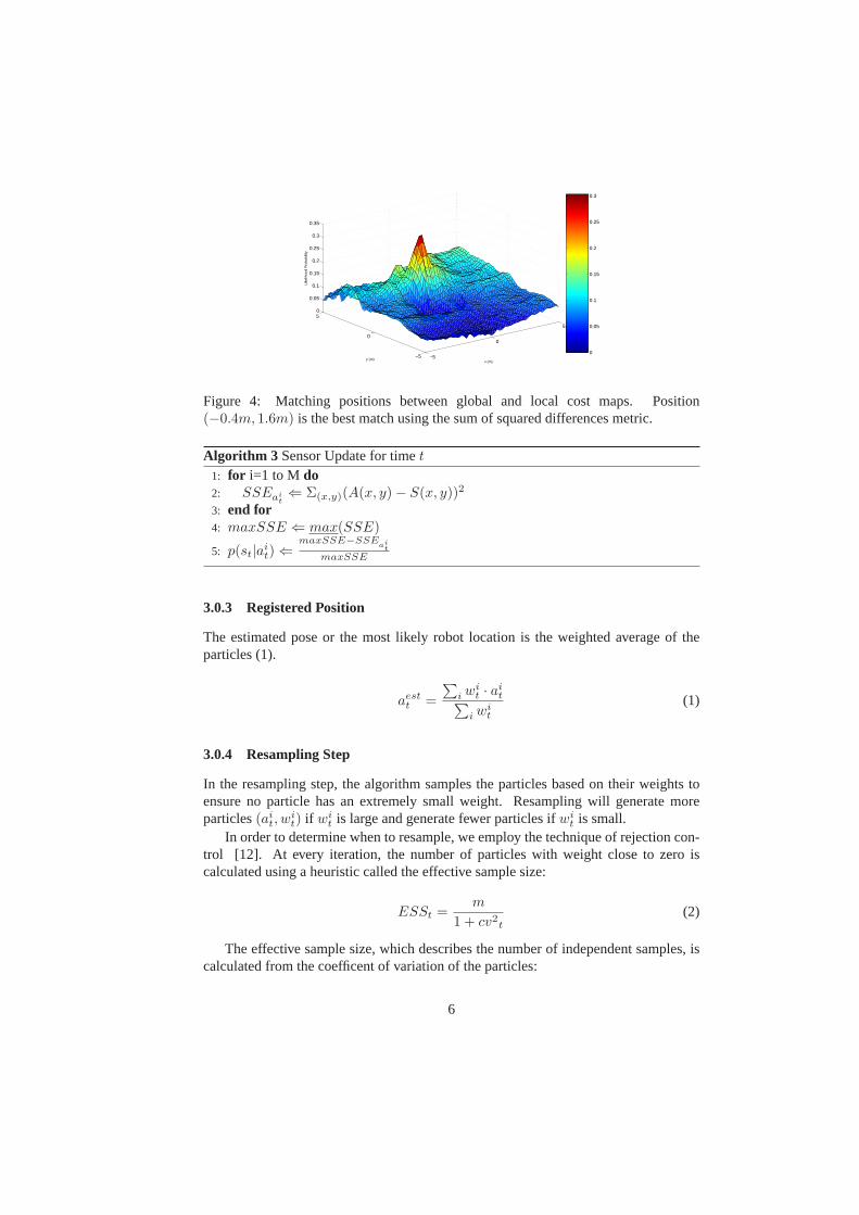
t) by taking the fraction of the difference valueover the maximum difference valuemaxSSE (Alg. 3 line 5). Using this similaritymetric, the larger the likelihood probability, the better the match. An example of aerror distribution generated from real data is shown in Fig.4. In this figure, there is aclear match around (-0.4m, 1.6m) indicating the most likelyvehicle position.
5
−5
0
5
−5
0
50
0.05
0.1
0.15
0.2
0.25
0.3
0.35
x (m)y (m)
Like
lihoo
d P
roba
bilit
y
0
0.05
0.1
0.15
0.2
0.25
0.3
Figure 4: Matching positions between global and local cost maps. Position(−0.4m, 1.6m) is the best match using the sum of squared differences metric.
Algorithm 3 Sensor Update for timet1: for i=1 to M do2: SSEai
t
⇐ Σ(x,y)(A(x, y) − S(x, y))2
3: end for4: maxSSE ⇐ max(SSE)
5: p(st|ait) ⇐
maxSSE−SSEa
it
maxSSE
3.0.3 Registered Position
The estimated pose or the most likely robot location is the weighted average of theparticles (1).
aestt =
∑i wi
t · ait∑
i wit
(1)
3.0.4 Resampling Step
In the resampling step, the algorithm samples the particlesbased on their weights toensure no particle has an extremely small weight. Resampling will generate moreparticles(ai
t, wit) if wi
t is large and generate fewer particles ifwit is small.
In order to determine when to resample, we employ the technique of rejection con-trol [12]. At every iteration, the number of particles with weight close to zero iscalculated using a heuristic called the effective sample size:
ESSt =m
1 + cv2t
(2)
The effective sample size, which describes the number of independent samples, iscalculated from the coefficent of variation of the particles:
6
cv2t =
var(wit)
E2(wit)
(3)
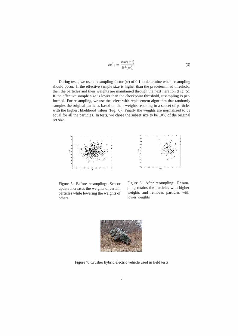
During tests, we use a resampling factor (α) of 0.1 to determine when resamplingshould occur. If the effective sample size is higher than thepredetermined threshold,then the particles and their weights are maintained throughthe next iteration (Fig. 5).If the effective sample size is lower than the checkpoint threshold, resampling is per-formed. For resampling, we use the select-with-replacement algorithm that randomlysamples the original particles based on their weights resulting in a subset of particleswith the highest likelihood values (Fig. 6). Finally the weights are normalized to beequal for all the particles. In tests, we chose the subset size to be 10% of the originalset size.
Figure 5: Before resampling: Sensorupdate increases the weights of certainparticles while lowering the weights ofothers
Figure 6: After resampling: Resam-pling retains the particles with higherweights and removes particles withlower weights
Figure 7: Crusher hybrid electric vehicle used in field tests
7
Figure 8: A priori cost map at 30cm resolution with a size of 974m by 806m. Theblack line represents the vehicle’s path through the terrain.
4 Results
The robot used for field testing was a large, six-wheeled vehicle equipped with laserrangefinders and cameras for on-board perception (Fig. 7). To test the algorithm,we used data collected from field tests conducted on off-roadterrain containing anassortment of vegetation, slopes, ditches, trees, and rocks. This data also included thetrue vehicle location collected using GPS. A path planner used the cost maps generatedfrom overhead and local data to find the lowest cost route through the terrain.
The map cost values range from0 to 65535 with 0 being unknown and65535 beingcompletely blocked. Lower cost indicate more traversable map cells. Because theon-board sensors and overhead mapping process differ significantly in data resolutionand occlusion properties, the extreme cost values (i.e., 0 and 65535) are discarded tofacilitate better matching.
Fig. 8 shows the area that the robot traversed. It contains both open areas with fewterrain features and dense areas with many more features. Wetested the localizationalgorithm in simulation on this area by ignoring the GPS information. We ran theexperiment on the tree-covered portion of the terrain, since a vehicle is most likelyto lose GPS in these areas; however, these areas are also likely to have unique costfeatures for matching.
During testing, the robot generated local maps with a 20cm resolution and a sizeof 24m by 24m. The robot was centered on each of the maps. The global map had a30cm resolution and was 974m by 806m in size. We initialized the algorithm with 484particles at the correct starting pose. We assumed that before the robot traveled into thetest region, GPS was available and position was known. Once the vehicle entered theregion, GPS became unavailable. In the map, this region starts at the upper left hand
8
side and continues down through the more feature-rich terrain, depicted by the blackpath. The localization algorithm was invoked once per meterof robot travel. Duringthe entire test run, the robot traveled approximately2.263 km in the x direction and2.072 km in the y direction giving a total distance of3.068 km.
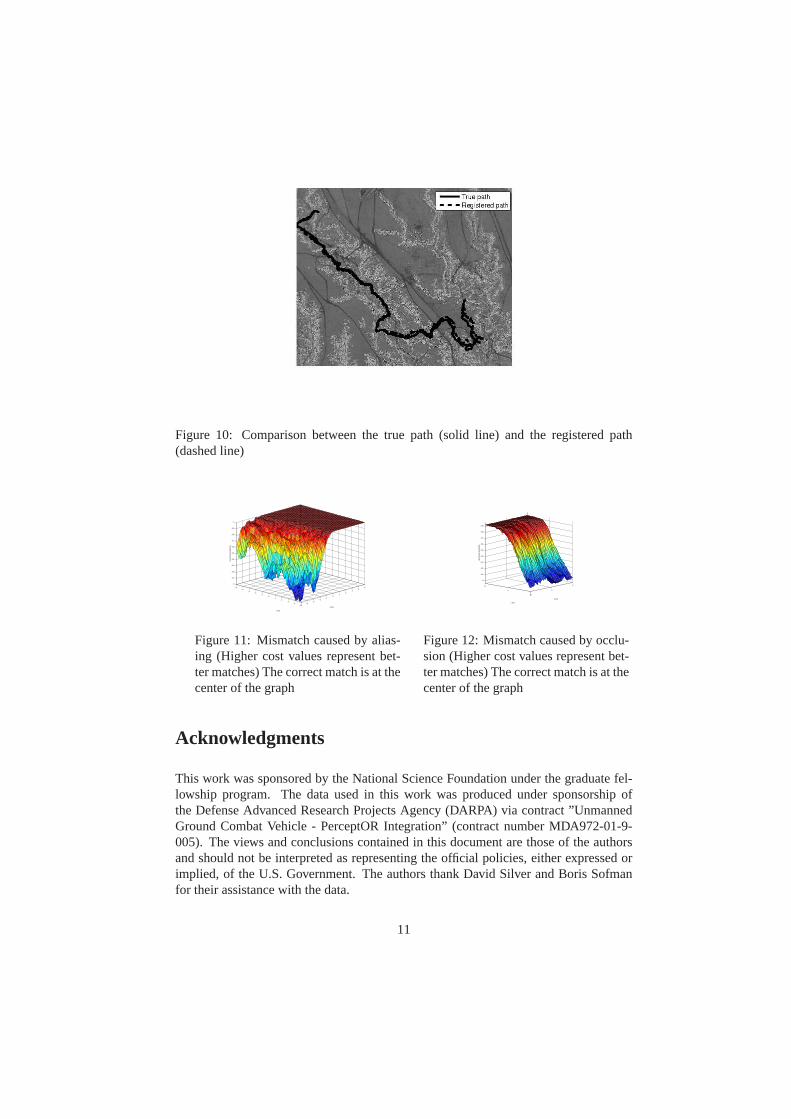
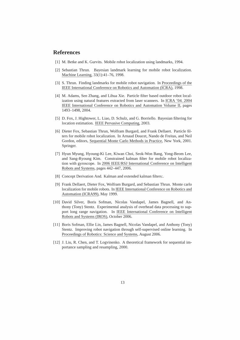
Fig. 9 shows the Euclidean distance between the estimated pose (producted fromsimulated experiments) and the correct pose (collected from the dataset) at each frame.While some frames benefit from registration, for other frames, localization errors arehigh. The estimated position deviates as little as 1m and as much as 45m from thetrue position of the robot (Fig. 10). One reason is due to ambigious matches in theregistration process particularly when the likelihood probability distribution appearsto be multi-modal. These ambiguities or aliasing effects lead to several high scor-ing matches between the sensor and overhead data as opposed to just one. In framescontaining the aliasing effects, the algorithm fails to choose the correct location. Aninstance of an aliasing effect occurs around frame 6000 where the scene is very sparsewith few features against which to register. The graph of theposition matches indicateseveral mismatches (Fig. 11). The particle filter could not recover from the mismatchesbecause the vehicle stayed in the open area for almost 200 cycles before reaching a re-gion with more distinct features. One way to solve this problem is to detect when thedistribution is multi-modal, select the best position using a heuristic, and renormalizethe particles based on the position selected. This method will mitigate aliasing effectsby removing the ambiguities from the data.
Localization errors also occur because of perspective effects and occlusion that arenot completely removed by the cost conversion. For instance, the global and localmaps at frame 4700 are shown in Fig. 13. While a high cost feature appears in theoverhead map (circled part), only a portion of the feature appear in the sensor map.The remainder of the feature is occluded making it difficult to match the data exactlydue to the missing part. This results in the registration returning an incorrect match.Whereas the global and local data should match at the center ofthe frame, the bestmatch using sum of squared difference at positions within a 10m by 10m square aroundthe true pose is at position(5m,−4m), 6.7 meters off (Fig. 12). However the particlefilter recovers from this mismatch because the large weightsfor the correct positionoffset the single mismatch. One way of further removing occlusion effects during thecost conversion process is to only use cost features that canbe measured easily in bothoverhead and sensor data. For instance, features such as trees would be disregardeddue to potentially large perspective differences.
Fig. 14 shows the position distributions between dead-reckoning plus registrationand dead-reckoning alone at the end of the test. While the dead-reckoning distributioncontains no bias, the standard deviation of the distribution is fairly large at 56.7m. Onthe other hand, the standard deviation of the localization distribution is much smaller,at 4.8m. The two standard deviations indicate that the uncertainty using only dead-reckoning is greater than the uncertainty using dead-reckoning plus registration. Inother words, dead-reckoning errors can grow up to 156m due toGaussian noise. How-ever, incorporating registration pushes the estimated vehicle position to be 35m awayfrom the correct position. This result arises because of thehigh number of map mis-matches that occur in the second half of the run. In this comparison, dead-reckoningpossesses zero bias because it is produced from simulation while the registration re-
9
1000 2000 4000 6000 8000 100004700 60000
5
10
15
20
25
30
35
40
45
50
Frame
Err
or (
m)
Figure 9: Registration error when compared to GPS ground truth at every frame
sults were obtained through experiments and therefore subject to bias due to positionmismatches.
One way to interpret the results is to use risk analysis to findthe amount of riskinvolved in each method. We consider risk as a weighted mean of a particular lossfunction:
riskt = ΣiL(ait) · w
it (4)
For instance, we analyzed the results using a popular loss function, the quadraticfunction L(x) = (ai
t − aestt )2. We chose this because we wanted to penalize more
for uncertainty in the estimate. Using the particles and their weights at the completionof the test run, the risk calculated for the localization results is31693.5 while the riskfor dead-reckoning is80688.01. Thus using this particular loss function, pure dead-reckoning is more than twice as risky as cost-based registration.
5 Conclusion
When GPS is absent, relying on dead-reckoning alone can be risky because the robotcan become lost in an environment due to error accumulation.Incorporating environ-mental information to help track the position of a vehicle can be very useful in robotlocalization. In this paper, we proposed a particle filter approach that uses mobilitycost maps to address the position tracking problem. Howevertwo main obstacles toperfect cost-based registration are aliasing and occlusion effects. Despite these issues,sample-based localization produces a position distribution with a much smaller losswhen compared to the distribution of pure dead-reckoning. Depending on the lossfunction used to analyze the risk of each approach, localization via registration mayperform better. Therefore, cost-based registration for robot localization is a promisingmethod for position tracking.
10
Figure 10: Comparison between the true path (solid line) andthe registered path(dashed line)
−5−4
−3−2
−10
12
34
5−5−4
−3−2
−10
12
34
5
0
0.1
0.2
0.3
0.4
0.5
0.6
0.7
0.8
0.9
1
y (m)
x (m)
Like
lihoo
d pr
obab
ility
Figure 11: Mismatch caused by alias-ing (Higher cost values represent bet-ter matches) The correct match is at thecenter of the graph
−5
0
5−5
0
5
0
0.1
0.2
0.3
0.4
0.5
0.6
0.7
0.8
0.9
y (m)
x (m)
Like
lihoo
d pr
obab
ility
Figure 12: Mismatch caused by occlu-sion (Higher cost values represent bet-ter matches) The correct match is at thecenter of the graph
Acknowledgments
This work was sponsored by the National Science Foundation under the graduate fel-lowship program. The data used in this work was produced under sponsorship ofthe Defense Advanced Research Projects Agency (DARPA) via contract ”UnmannedGround Combat Vehicle - PerceptOR Integration” (contract number MDA972-01-9-005). The views and conclusions contained in this document are those of the authorsand should not be interpreted as representing the official policies, either expressed orimplied, of the U.S. Government. The authors thank David Silver and Boris Sofmanfor their assistance with the data.
11
Figure 13: The bottom left cost map gives the overhead view ofthe area at frame4700. The bottom right cost map gives a ground view of the samearea. The twocircles indicate a feature that shows up fully in the overhead view, but is occluded inthe ground view. Lighter colors indicate higher cost.
−300 −200 −100 0 100 200 3000
0.02
0.04
0.06
0.08
0.1
0.12
0.14
x (m)
Pro
babi
lity
(nor
mal
ized
)
RegistrationPure dead−reckoning
Figure 14: Position distributions of particles resulting from registration and dead-reckoning
12
References
[1] M. Betke and K. Gurvits. Mobile robot localization usinglandmarks, 1994.
[2] Sebastian Thrun. Bayesian landmark learning for mobilerobot localization.MachineLearning, 33(1):41–76, 1998.
[3] S. Thrun. Finding landmarks for mobile robot navigation. In Proceedingsof theIEEE InternationalConferenceonRoboticsandAutomation(ICRA), 1998.
[4] M. Adams, Sen Zhang, and Lihua Xie. Particle filter based outdoor robot local-ization using natural features extracted from laser scanners. In ICRA ’04. 2004IEEE InternationalConferenceon Roboticsand AutomationVolume II, pages1493–1498, 2004.
[5] D. Fox, J. Hightower, L. Liao, D. Schulz, and G. Borriello. Bayesian filtering forlocation estimation.IEEEPervasiveComputing, 2003.
[6] Dieter Fox, Sebastian Thrun, Wolfram Burgard, and FrankDellaert. Particle fil-ters for mobile robot localization. In Arnaud Doucet, Nandode Freitas, and NeilGordon, editors,SequentialMonteCarloMethodsin Practice, New York, 2001.Springer.
[7] Hyun Myung, Hyoung-Ki Lee, Kiwan Choi, Seok-Won Bang, Yong-Beom Lee,and Sang-Ryoung Kim. Constrained kalman filter for mobile robot localiza-tion with gyroscope. In2006IEEE/RSJInternationalConferenceon IntelligentRobotsandSystems, pages 442–447, 2006.
[8] Concept Derivation And. Kalman and extended kalman filters:.
[9] Frank Dellaert, Dieter Fox, Wolfram Burgard, and Sebastian Thrun. Monte carlolocalization for mobile robots. InIEEEInternationalConferenceonRoboticsandAutomation(ICRA99), May 1999.
[10] David Silver, Boris Sofman, Nicolas Vandapel, James Bagnell, and An-thony (Tony) Stentz. Experimental analysis of overhead data processing to sup-port long range navigation. InIEEE InternationalConferenceon IntelligentRobotsandSystems(IROS), October 2006.
[11] Boris Sofman, Ellie Lin, James Bagnell, Nicolas Vandapel, and Anthony (Tony)Stentz. Improving robot navigation through self-supervised online learning. InProceedingsof Robotics:ScienceandSystems, August 2006.
[12] J. Liu, R. Chen, and T. Logvinenko. A theoretical framework for sequential im-portance sampling and resampling, 2000.