Cost Effective Design of RC Building FrameEmploying Uni�ed Particle Swarm OptimizationPayel Chaudhuri  ( payelce@gmail.com )

Indian Institue of Technology, Kharagpur https://orcid.org/0000-0003-2214-9554Swarup Barman 

Indian Institute of Technology KharagpurDamodar Maity 

Indian Institute of Technology KharagpurDipak Kumar Maiti 

Indian Institute of Technology Kharagpur

Research Article

Keywords: cost effective design, uni�ed particle swarm optimization, STAAD Pro, RC building frame, windload, seismic load.

Posted Date: April 28th, 2021

DOI: https://doi.org/10.21203/rs.3.rs-227713/v1

License: This work is licensed under a Creative Commons Attribution 4.0 International License.  Read Full License

1

Cost effective design of RC building frame employing unified particle 1

swarm optimization 2

Payel Chaudhuri1, Swarup K. Barman2, Damodar Maity1, Dipak K. Maiti2 3

1Civil Engineering Department, Indian Institute of Technology, Kharagpur -721302, India, 4

payelce@gmail.com 5

2Aerospace Engineering Department, Indian Institute of Technology, Kharagpur -721302, 6

India. 7

8

ABSTRACT 9

Present paper deals with the cost effective design of reinforced concrete building frame 10

employing unified particle swarm optimization (UPSO). Two building frames with G+8 11

stories and G+10 stories have been adopted to demonstrate the effectiveness of the present 12

algorithm. Effect of seismic loads and wind load have been considered as per Indian Standard 13

(IS) 1893 (Part-I) and IS 875 (Part-III) respectively. Analysis of the frames has been carried 14

out in STAAD Pro software. The design loads for all the beams and columns obtained from 15

STAAD Pro have been given as input of the optimization algorithm. Next, cost optimization 16

of all beams and columns have been carried out in MATLAB environment using UPSO, 17

considering the safety and serviceability criteria mentioned in IS 456. Cost of formwork, 18

concrete and reinforcement have been considered to calculate the total cost. Reinforcement of 19

beams and columns has been calculated with consideration for curtailment and feasibility of 20

laying the reinforcement bars during actual construction. The numerical analysis ensures the 21

accuracy of the developed algorithm in providing the cost optimized design of RC building 22

frames considering safety, serviceability and constructional feasibilities.Further, Monte Carlo 23

simulations performed on the numerical results, proved the consistency and robustness of the 24

developed algorithm. Thus, the present algorithm is capable of giving a cost effective design 25

of RC building frame, which can be adopted directly in construction site without making any 26

changes. 27

28

2

Key words: cost effective design, unified particle swarm optimization, STAAD Pro, RC 29

building frame, wind load, seismic load. 30

1. Introduction 31

Reinforced concrete is a dominant material for constructing various civil engineering 32

structures due to its high compressive strength, durability and resistance to damage from fire 33

and water. Conventional trial and error based design of RC structures is based on only safety 34

criteria, and requires excessive materials. Thus construction costs of building increases. So, 35

increase in use of reinforcement concrete comes with the demand for economical design. 36

Thus, from last few decades, researchers have proposed different method for cost 37

optimization of RC frames. Increase in computational power of computers has enhanced the 38

willfulness of such attempts drastically. Main challenge in optimizing the RC structures are 39

number of optimizing variables in comparison with the optimal design of steel structures, 40

where only material is considered for entire structures and cost of the entire structure is 41

proportional to weight of that material. On the other hand, cost of RC structures consist of 42

cost of concrete, cost of steel reinforcement and cost of formworks. Their unit costs differ 43

from each other. Their inter-relations are not simple, because any two of them change 44

significantly with slight changes in the quantity of the third factor. This in turn changes the 45

total cost of RC frame to a great extent. Thus, the actual problem comes to finding 46

appropriate combination of values for three aforementioned components of costs without 47

violating the safety requirements so that the total cost becomes minimum. Again, RC sections 48

are cast in situ. So, while designing cost effective sections, size of the sections and 49

reinforcement detailing should be provided to meet the specific demands from architectural 50

and construction point of view. Thus, presence of all these factors along with constraints 51

regarding strength, serviceability, architectural demands and easiness of construction make 52

cost optimization of real life RC structures a highly cumbersome task. However, in the same 53

time an algorithm to optimize the cost of a RC building frame satisfying all the necessary 54

criteria will be a valuable tool to the design practitioner. 55

Despite all these challenges many researchers have tried to find cost optimize designs of 56

RC building components. Milajić et al. [1] reviewed various methods available in literatures 57

for optimal design of reinforced concrete structure. They focused on the problems of these 58

existing methodologies, such as: gap between the theory and practice in the field, lack of 59

universal criteria and standard benchmark problem etc.Also, when ones talks about of cost 60

3

optimized design of a complete RC building project, it includes optimizing the topology of 61

the building, material costs of the building components, reinforcement distribution, cost of 62

shuttering, labor cost maintaining all the safety guidelines of competent authority. 63

Topology optimization of building means finding out optimum layout of the building for 64

a particular project. Topology optimization is avery popular and common term in steel 65

structures, where topology of truss is optimized to achieve cost optimum design [2]. 66

However, researchers also tried to implemented the concept of topology optimization also in 67

case of concrete structures by various means, such as windowed evolutionary structural 68

optimization (WESO) [3], plastic design layout optimization technique [4], dynamic 69

programming utilizing genetic algorithm (GA) based multi objective optimization [5]. Apart 70

from that, Zegard et al. [6] have implemented three different methods of topology design 71

optimization in building engineering. However, in real project topology is not decided solely 72

based oncost only. There are other deciding factor such as utility of the building, aesthetic 73

beauty or client’s wish. Labor cost depend on the location of the construction and days 74

required to finish the construction. This can be managed with proper 75

constructionmanagement and planning strategies like Critical Path Method (CPM) and 76

Project Evaluation and Review Technique (PERT). Thus, present study is focused on the 77

optimizing the design of the structural components of a building frame. 78

Structural components, such as, beams, columns, slab and foundation contribute most in 79

the total cost of a project. Thus, cost optimum design of structural components are of utmost 80

important for minimizing the project cost. Cost optimum design of RC beams have been 81

attempted by researchers utilizing various methods, simplex and Lagrangian optimization 82

method [7], geometric programming [8], GA based algorithm [9, 10], polynomial 83

optimization technique [11], simulated annealing [12], random search technique (RST) [13], 84

charged system search (CSS) [14]. Cost optimum design of T-beams [15]andCost optimum 85

design RC columns [7, 16, 17] also have been attempted. Apart from beam and column 86

optimization, design of reinforced concrete (RC) flat slabs have also been optimized by 87

Aldwaik and Adeli [18] using Neural dynamic model for Adeli and Park (NDAP) [19], 88

Design optimization of RC foundation has been performed by Chaudhuri and Maity [20]. 89

Besides these individual structural components researchers have also tried to optimize the 90

beam-column frames in terms of weight [21], in terms of cost [22-29]. All these studies 91

regarding design optimization of RC building components or frames are conformed to the 92

4

guidelines decided by the various standards of different countries such as Indian standard (IS 93

456)[7,11, 20, 26], American standard (ACI 318, ASCE7)[13,17, 21-25, 28, 29], European 94

standard (Eurocode 2) [15,27]and Australian standard (AS 3600) [14], Brazilian standard 95

(NBR 6118)[12]. Apart from these, RazmaraShooli et al. [30] have proposed a GA-PSO 96

based algorithm for performance-based design optimization of a special moment-resisting 97

frames based on guidelines provided by American standards (ATC-40, FEMA 356, ASCE-7 98

and ASCE-41).In these literatures the researchers used geometry of beam, column, amount of 99

reinforcement, cost of material and shuttering as their optimization variable.In the problems 100

regarding optimized design of RC components, optimizing the distribution of reinforcement 101

are also an important issue [31, 32]. 102

While solving any optimization problems choosing proper optimization techniques is 103

utmost important, every optimization techniques have their strengths and weaknesses. In this 104

regard, it is important to have an idea about the optimization techniques used by the 105

predecessors to solve a particular class of problems. The cost optimization design problems 106

of RC frames have been tackled by the researchers by using various optimization techniques. 107

Few of them have already been discussed earlier in this section. However, reviews of the 108

optimization algorithms used by researchers have been presented in Table 1 for clarity. 109

Thus, the key points, which have been observed from the above literature are as follows: 110

i) Literature studying the cost-optimum design of RC building are quite less in 111

number. 112

ii) Most of the literatures are focused on the optimization of only a particular 113

member (beam or column), and reinforcement detailing pattern of beam or column 114

sections. 115

iii) Also, no algorithm from above literature have been tested for large scale multi-116

storey building frame to provide cost optimized design accompanied by 117

construction friendly reinforcement detailing. 118

iv) Usage of optimization techniques in this field is also very less compared to other 119

fields like structural health monitoring, travelling salesman problems, water 120

resource etc. 121

5

Apart from above points another important issue is the shortcomings of commercial 122

design software. Although, design performed in the software is correct in term of safety 123

criteria, they provide the reinforcement amount in terms area instead construction friendly 124

reinforcement detailing. Thus, the method developed in the present studyaims towards 125

alleviate these shortcomings. Also Unified Particle Swarm Optimization has not been used 126

asa cost optimization method for multistory building design in the previous studies, although 127

it has been used very effectively in cost optimization of RC foundation [20], damage 128

detection problems [33-38], magnetoencephalography problem [39] etc. Hence, UPSO have 129

been found to the appropriate optimization method for multistory building design and cost 130

optimization. Thus, main objective of the present paper is to develop cost-optimized design 131

algorithm for RC frames following the safety and serviceability requirements of IS 456 [40] 132

employing UPSO. Efficiency of the algorithm has been shown using two building frames 133

(G+8, and G+10) of different planner configurations. Effects of seismic and wind load also 134

have been considered. Optimization has been performed based on minimum cost rather than 135

minimum weight, as the considered building frames are not high-rise (Prakash et al. [7]). 136

Final optimized sections and reinforcement details obtained from the present algorithm can 137

be used without altering in the actual site during construction phase.The efficiency of the 138

developed design optimization algorithm has been investigated using Monte Carlo 139

simulation. Monte Carlo method estimates the probability of favorablesolution of the 140

developed optimization algorithm when a large number of experiments are carried out for 141

cost optimization of both the buildings. This consequently evaluates the robustness of the 142

developed algorithm in case of huge number of experiments and different types of buildings. 143

2. Mathematical formulation 144

An UPSO based algorithm has been developed in the present study to obtain cost 145

effective design of the multi-storeyed reinforcement concrete frame. Details of structural 146

analysis, design criteria, optimization algorithm, objective functions have been discussed in a 147

brief manner in this section. 148

2.1. Structural analysis 149

In general building frames are subjected to gravity load (dead load (DL) and live load 150

(LL)), wind load (WL) and seismic load (SL). Designers use all these loads in various 151

combinations to calculate design forces such as axial loads, bending moments and shear 152

6

forces for beams and columns. The moments, shear forces and axial loads for the critical load 153

combination are used to design the beams and columns of the building frames. Detail 154

procedure for analysis of building frames under aforementioned loads is mentioned briefly in 155

the subsequent sections. 156

2.1.1. Gravity loads 157

Gravity loads consist of dead load and live load. Dead load of different components of a 158

building can be considered as per IS 875 (Part I) [41]. Dead loads constitute of the following 159

loads. 160

1. Self-weight of beams and columns. 161

2. Self-weight of internal and external wall and parapet wall. 162

3. Self-weight of floor slabs. 163

4. Dead load coming from floor finish and plastering 164

Any temporary or transient loads which act on the building can be defined as live loads. 165

People, furniture, vehicles, and almost everything else that can be moved throughout a 166

building come under live loads. Live loads can be provided to any structural element (floors, 167

columns, beams, even roofs). Appropriate amount and type of live load can be decided based 168

on the specification given on IS 875 (Part II) [42]. 169

2.1.2. Wind loads 170

Wind load should be considered for designing a multi-storey building frame.The nature 171

of flow of wind past a body resting on a surface depends on the conditions of the surface, the 172

shape of the body, its height, velocity of wind flow and many other factors [43]. IS 875 (Part 173

III) [44] contains the guidelines for considering the effects of wind on a multistorey building. 174

The shape of wind load velocity profile is similar to boundary layer flow profile.A typical 175

velocity profile of wind load considered for analysis has been shown in Fig. 1. The dotted 176

line represents boundary layer. In general velocity is zero at the ground and increases up to 177

the boundary layer. Beyond boundary layer wind velocity does not changes with height. As 178

the wind travel in upstream direction through a particular terrain, the wind profile changes 179

and velocity and height of boundary layer increases. The distance travelled by a wind profile 180

7

on a particular terrain is called fetch length, i.e. x1 and x2 in Fig. 1. Upward penetration of the 181

velocity profile at any fetch length is called developed height, i.e., h1 and h2 in 182

Fig.1.Developed height increases up to gradient height, where velocity become maximum. 183

After that even if wind travel upstream direction velocity profile remain unchanged. At this 184

point it can said that velocity profile is fully developed for that particular terrain. In case of 185

wind analysis of a structures generally it is assumed that wind profile is fully developed 186

before hitting the structure. The values of a fully developed velocity profile depends on the 187

terrain category. As the terrain category becomes rougher, gradient height increases. IS 875 188

(Part III) [44] have provided the multiplier for velocity profile for each terrain category. 189

Initially wind analysis of any structure starts with selecting proper basic wind speed 𝑉𝑏 190

depending on the location of the structure. The design wind speed 𝑉𝑧at height 𝑧 in m/s can be 191

calculated mathematically as per Eq. 1. 192

𝑉𝑧 = 𝑉𝑏𝑘1𝑘2𝑘3𝑘4 (1)

Here, 𝑘1 is risk factor or probability factor. It is decided based on design life of structures. 193 𝑘2is the velocity profile multiplier based on the terrain category. 𝑘3 is topography factor, 194

decided based on the ground slope of the site. 𝑘4is a factor based on the cyclonic importance 195

of the structure. 196

The wind pressure in N/m2 at any height 𝑧 above the mean ground level can be obtained 197

from the following Eq. 2. 198

𝑝𝑧 = 0.6𝑉𝑧2 (2)

Finally design wind pressure (𝑝𝑑) in N/m2 at any height 𝑧 above the mean ground level 199

can be obtained from the following Eq. 3. 200

𝑝𝑑 = 𝐾𝑑𝐾𝑎𝐾𝑐𝑝𝑧, 𝑝𝑑 ≥ 0.7𝑝𝑧 (3)

Design moment, shear and axial forces in beams and columns for wind load are calculated by 201

applying the design wind pressure on the frame. 202

2.1.3. Seismic loads 203

8

When, any structure is subjected to seismic load dynamic equation of the structure can be 204

represented as Eq. 4. 205

[𝑀]�̈�(𝑡) + [𝐶]�̇�(𝑡) + [𝐾]𝑥(𝑡) = −[𝑀]𝑢�̈�(𝑡) (4)

Where, [𝑀], [𝐶] and [𝐾] are mass, damping and stiffness matrix of the structure. 𝑢�̈�(𝑡)is the 206

acceleration time history of the induced earthquake. 𝑥(𝑡)is the time history response of the 207

structure due to the induced earthquake force. Equation 4 can be solved using numerical 208

approaches for time history responses, such as displacement 𝑥(𝑡), velocity �̇�(𝑡) and 209

acceleration �̈�(𝑡). Eventually stress time history also can be obtained. But, there are some 210

difficulties to do an actual seismic analysis for every structure to be designed. They are 211

i) It is not always possible to have the earthquake acceleration time history of the 212

exact location of the structure. 213

ii) Analysis of the structure cannot be carried out solely considering the peak ground 214

acceleration (PGA) of the earthquake, as the response of the structure depends on 215

the frequency component of the earthquake and its own dynamic properties. 216

These difficulties can be overcome by using the response spectrum of the earthquake instead 217

of using the acceleration time history as input. Response spectrum represents the maximum 218

response of damped single degree of freedom (SDOF) system for a particular input 219

earthquake motion at different natural period. Maximum response is more important to a 220

designer than the entire time history. One can also obtain mean response spectrum for a 221

particular location using more than one data of past earthquakes of the location. Also, use of 222

different damping value will give different response spectrum for same earthquake response. 223

Once acceleration response spectrum is known, one can easily obtain the maximum base 224

shear simply by multiplying the spectral acceleration obtained from the response spectrum 225

with the seismic mass of the structure. Every country develops their own design response 226

spectrum based on the past earthquake happenings in the region. In general seismic design 227

practice the structure should prevent non-structural damage for minor earthquake, prevent 228

structural damage with minimum non-structural damage for moderate earthquake and avoid 229

collapse to save lives in case of a major earthquake. Thus, no one use the spectral 230

acceleration associated with PGA (maximum considered earthquake (MCE)) for seismic 231

9

design of structure. Rather, the analysis is carried out for a much reduced value of spectral 232

acceleration (design basis earthquake (DBE)). 233

The guidelines for analyzing a building frame for seismic loading is mentioned in IS 234

1893(Part-I)[45]. Instead of solving rigorous dynamic equations, Indian standard has 235

provided simple linear static approach for simple regular structures utilizing the response 236

spectrum. Entire country has been divided into four seismic zone (II, III, IV, V) based on the 237

PGA. Seismic forces has two horizontal and one vertical components. For simple regular 238

building frame vertical component is ignored. The design horizontal seismic coefficient (𝐴ℎ) 239

can be calculated as Eq. 5. 240

𝐴ℎ = (𝑍2) (𝑆𝑎𝑔 )(𝑅𝐼 )

(5)

Here, 𝑍 is seismic zone factor depend on the seismic zone of the location of the structures. In 241

the term (𝑍2), (12) factor used to reduce the MCE to DBE.𝐼is the importance factor, decided 242

based on the occupancy and use of the structure. 𝑅is the response reduction factor depends on 243

the ductility, redundancy and overstrength of the structure. A structure with good ductility 244

will have high value of 𝑅, i.e., that structure will be designed for low seismic force. (𝑆𝑎𝑔 )is 245

normalize spectral acceleration coefficient, which can be calculated based on the natural 246

period of the structure and soil type from the design response spectrum presented in the 247

standard (Fig. 2). 248

The natural period of ordinary RC building can be calculated from Eq. 6. 249

𝑇𝑎 = 0.09𝐻𝑏𝑙√𝐷𝑏𝑙 (6)

Now, the base shear can be computed for the building as a whole from the following 250

equation (Eq. 7). 251

𝑉𝐵 = 𝐴ℎ𝑊 (7)

10

where, 𝑊 is the seismic weight of the building which is calculated by adding full dead load 252

and 25 percent of the liveload. 253

The base shear in Eq.7 is distributed at the center of mass of all the floor levels of the frame. 254

These forces are distributed to the individual lateral load resisting elements through structural 255

analysis considering floor diaphragm action. 256

2.1.4. Load combinations 257

All the above loads are considered for suitable load combinations according toIS 875 258

(Part V)[46] with appropriate load factors. The load combinations have been mentioned 259

below 260

1. 1.5(DL + LL) 261

2. 1.5(DL± WL) 262

3. (0.9DL±1.5WL) 263

4. 1.5(DL± SL) 264

5. (0.9DL±1.5SL) 265

6. 1.2(DL+LL±WL) 266

7. 1.2(DL+LL±SL) 267

Among all these load combinations only most critical load combination has been used for 268

designing each beam and column of the building frames. 269

2.2. Structural design 270

Beams and columns of all the frames were designed adopting Limit State Method as per 271

the guidelines provided in the Indian Standard IS 456 [40] in the present study. The design 272

procedure has been described briefly in the following sections. 273

2.2.1. Beam design 274

The design of beam is carried out based on limit state of collapse in flexure considering 275

plane section normal to the axis remains plane after bending. Longitudinal reinforcements in 276

11

beams are provided to carry bending moments, whereas stirrups are provided to carry shear 277

forces. Design bending moment (𝑀𝑢) and shear forces (𝑉𝑢) for all beam sections are obtained 278

from the structural analysis. At first the beam is designed to carry design bending moment. 279

The limiting moment of resistance of balanced singly reinforced beam section due to flexure 280

can be calculated as per Eq. 8. 281

𝑀𝑢,𝑙𝑖𝑚 = 0.36 𝑥𝑢𝑚𝑎𝑥𝑑𝑒 (1 − 0.42 𝑥𝑢𝑚𝑎𝑥𝑑𝑒 ) 𝑏𝑑𝑒2𝑓𝑐𝑘 (8)

If 𝑀𝑢 ≤ 𝑀𝑢,𝑙𝑖𝑚, then the beam section is designed as singly reinforced section. The required 282

area of tensile reinforcement can be calculated from equation Eq. 9. 283

𝑀𝑢 = 0.87𝑓𝑦𝐴𝑠𝑡𝑑𝑒 𝑥𝑢𝑚𝑎𝑥𝑑𝑒 (1 − 𝑓𝑦𝐴𝑠𝑡𝑏𝑑𝑒𝑓𝑐𝑘), 𝐴𝑠𝑡 ≥ 0.85𝑏𝑑𝑒/𝑓𝑦 (9)

If 𝑀𝑢 > 𝑀𝑢,𝑙𝑖𝑚, then the beam is designed as doubly reinforced section. Area of tensile 284

reinforcement (𝐴𝑠𝑡1) required for 𝑀𝑢,𝑙𝑖𝑚 is calculated from equation Eq. 9. The area of 285

compression reinforcement for the excess moment i.e. ( 𝑀𝑢 − 𝑀𝑢,𝑙𝑖𝑚) is obtained from Eq. 286

10. 287

𝑀𝑢 − 𝑀𝑢,𝑙𝑖𝑚 = 𝑓𝑠𝑐𝐴𝑠𝑐(𝑑𝑒 − 𝑑′) (10)

where, 𝑓𝑠𝑐 =design stress in compression reinforcement and it is obtained from Table I 288

(Appendix III) corresponding to a strain of 0.0035 (𝑥𝑢𝑚𝑎𝑥−𝑑′)𝑥𝑢𝑚𝑎𝑥 , 𝑥𝑢𝑚𝑎𝑥𝑑𝑒 =0.53, 0.48, 0.46 for 289 𝑓𝑦 = 250, 415, 500 respectively. The area of corresponding tensile reinforcement (𝐴𝑠𝑡2) for 290

the excess moment(𝑀𝑢 − 𝑀𝑢,𝑙𝑖𝑚) is calculated in Eq. 11. 291

𝐴𝑠𝑡2 = 𝑓𝑠𝑐𝐴𝑠𝑐/0.87𝑓𝑦 (11)

longitudinal reinforcement of beams are provided based on 𝐴𝑠𝑡, 𝐴𝑠𝑡1, 𝐴𝑠𝑡2.Next, the provide 292

beam section is checked for design shear force. Nominal shear stress for beam section shall 293

be obtained from the following Eq. 12. 294

𝜏𝑣 = 𝑉𝑢/𝑏𝑑𝑒 (12)

12

The design shear strength 𝜏𝑐of concrete is calculated from IS 456 [40] or Appendix IIIfor 295

grade of concrete and percentage of total tensile reinforcement provided.If 𝜏𝑣 ≤ 𝜏𝑐, minimum 296

shear reinforcement shall be provided as per in Eq. 13. 297

𝑠𝑣 = min (0.87𝑓𝑦𝐴𝑠𝑣0.4𝑏 , 3𝑑𝑒 , 300 𝑚𝑚) (13)

If𝜏𝑐 < 𝜏𝑣 < 𝜏𝑐𝑚𝑎𝑥, The shear reinforcement should be designed to carry a shear force 𝑉𝑢𝑠 =298 𝑉𝑢 − 𝜏𝑐𝑏𝑑𝑒. 𝜏𝑐𝑚𝑎𝑥 can be obtained from IS 456 depending on the strength of the concrete. 299

(Table II, Appendix III) The spacing of the shear reinforcement shall be provided as obtained 300

from the following equation. Eq. 14. 301

𝑠𝑣 = min (0.87𝑓𝑦𝐴𝑠𝑣𝑑𝑒𝑉𝑢𝑠 , 0.87𝑓𝑦𝐴𝑠𝑣0.4𝑏 , 3𝑑𝑒 , 300 𝑚𝑚) (14)

Once the longitudinal reinforcement and shear reinforcement had been designed, the beam 302

should be checked to be safe against the serviceability criteria of limit state method. Thus, 303

maximum deflection of the beam should be within the limit provided by the design standard. 304

The total deflection of beam is thus calculated as per Eq. 15. 305

𝑎𝑡𝑑 = 𝑎𝑠 + 𝑎𝑐𝑠 + 𝑎𝑐𝑐 (15)

where, 𝑎𝑠 is calculated for the usual method for elastic deformation theory using short term 306

elasticity modulus 𝐸𝑐 and effective moment of inertia 𝐼𝑒𝑓𝑓 given in Eq. 16. 307

𝐼𝑟1.2−𝑀𝑟𝑀 𝑧𝑑𝑒(1− 𝑥𝑑𝑒)𝑏𝑤𝑏𝑏 , 𝐼𝑟 < 𝐼𝑒𝑓𝑓 𝐼𝑒𝑓𝑓 =< 𝐼𝑔𝑟 (16)

where, 𝑀𝑟 = 𝑓𝑐𝑟𝐼𝑔𝑟/𝑦𝑡, 𝑎𝑐𝑠is the deflection due to shrinkage and it is calculated according to 308

the equation Eq. 17. 309

𝑎𝑐𝑠 = 𝑓3𝜑𝑐𝑠𝑙2 (17)

13

where, 𝜑𝑐𝑠 = 𝑓4 ∈𝑐𝑠𝐷 , where, 𝑓3, 𝑓4 are calculated from IS 456 [40] annex C-3.1. (Appendix 310

III). ∈𝑐𝑠=0.0003.𝑎𝑐𝑐is the deflection due to creep for permanent loads and is defined in Eq. 311

18. 312

𝑎𝑐𝑐 = 𝑎𝑖,𝑐𝑐 − 𝑎𝑖 (18)

where, 𝑎𝑖,𝑐𝑐 is the initial plus creep deflection due to permanent loads obtained using an 313

elastic analysis with an effective modulus of elasticity (𝐸𝑐𝑒 = 𝐸𝑐/(1 + 𝜃)). 314

2.2.2. Column design 315

The design of column is done based on the same assumption for limit state of collapse in 316

flexure i.e. plane section normal to the axis remains plane after bending. All compression 317

members should be designed for a minimum eccentricity of load in two principal direction. 318

Minimum eccentricity in design of columns can be obtained from Eq. 19. 319

𝑒𝑚𝑖𝑛 = min ( 𝑙𝑐500 + 𝐷𝑐30 , 20 𝑚𝑚) (19)

All the column sections are designed considering combined effects of axial load and biaxial 320

bending moments. Thus, minimum eccentricity should be checked for both x and y direction 321

bending separately. If the column is subjected to axial load 𝑃𝑢, biaxial moments 𝑀𝑢𝑥 and 322 𝑀𝑢𝑦, the column section thus designed should satisfy for interaction ratio given by Eq. 20. 323

( 𝑀𝑢𝑥𝑀𝑢𝑥1)𝛼𝑛 + ( 𝑀𝑢𝑦𝑀𝑢𝑦1)𝛼𝑛 ≤ 1.0 (20)

𝛼𝑛is the exponent component whose value depends on 𝑃𝑢/𝑃𝑢𝑧. 𝛼𝑛 = 1for 𝑃𝑢/𝑃𝑢𝑧 ≤324 0.2. 𝛼𝑛 = 2for 𝑃𝑢/𝑃𝑢𝑧 ≥ 0.8. Linear interpolation should be used for intermediate values. 325 𝑃𝑢𝑧is calculated from Eq. 21. 326

𝑃𝑢𝑧 = 0.45𝑓𝑐𝑘 Ac + 0.75𝑓𝑦𝐴𝑠𝑐𝑐 (21)

𝑀𝑢𝑥1, 𝑀𝑢𝑦1 are the maximum uniaxial moment carrying capacity of the column section 327

combined with the axial load 𝑃𝑢 respectively for about 𝑥 and 𝑦 direction. Now, while 328

14

considering any particular direction bending two different cases can emerge based on the 329

position of the neutral axis as shown in Fig. 3. 330

Case 1: When the neutral axis lies within the column section (Fig. 3b), the axial load 331

carrying capacity and moment carrying capacity of the section can be calculated from Eq. 22 332

and Eq. 23 respectively. 333

𝑃𝑢1 = 0.36𝑘𝑓𝑐𝑘𝑏𝑐𝐷𝑐 + ∑ 𝑝𝑖𝑏𝑐𝐷𝑐100 ∗ (𝑓𝑠𝑖 − 𝑓𝑐𝑖)𝑛𝑖=1

(22)

𝑀𝑢1 = 0.36𝑘𝑓𝑐𝑘𝑏𝑐𝐷𝑐2(0.5 − 0.416𝑘) + ∑ 𝑝𝑖𝑏𝑐𝐷𝑐100 ∗ (𝑓𝑠𝑖 − 𝑓𝑐𝑖)𝑛𝑖=1 𝑦𝑖

(23)

where 𝑘 = 𝑥𝑢/𝐷; 334

Case 2: If neural axis lies outside the column section (Fig. 3c) the axial load carrying 335

capacity and moment carrying capacity of the section can be calculated from Eq. 24 and Eq. 336

25 respectively. 337

𝑃𝑢1 = 𝐶1𝑓𝑐𝑘𝑏𝑐𝐷𝑐 + ∑ 𝑝𝑖𝑏𝑐𝐷𝑐100 ∗ (𝑓𝑠𝑖 − 𝑓𝑐𝑖)𝑛𝑖=1

(24)

𝑀𝑢1 = 𝐶1𝑓𝑐𝑘𝑏𝑐𝐷𝑐(0.5𝐷𝑐 − 𝐶2𝐷𝑐) + ∑ 𝑝𝑖𝑏𝑐𝐷𝑐100 ∗ (𝑓𝑠𝑖 − 𝑓𝑐𝑖)𝑛𝑖=1 𝑦𝑖

(25)

where,𝑓𝑐𝑖 is stress in concrete at the level of i-th row of reinforcement and can be calculated 338

from Fig. 3d. 𝑓𝑠𝑖 is stress in the i-th row of reinforcement can be obtained from Table III 339

(Appendix III). 𝐶1 is stress co-efficient and 𝐶2𝐷 is the distance of the centroid the concrete 340

stress block (Fig. 3d) measured from the highly compressed edge. 𝐶1 and 𝐶2can be obtained 341

from Eq. 26 and Eq. 27 respectively. 342

𝐶1 = Astr𝑓𝑐𝑘𝐷𝑐 (26)

15

𝐶2 = 𝑀𝑐/Astr (27)

𝐴𝑠𝑡𝑟is the area of the stress block (Fig.3d), and can be calculated from the Eq. 28. 343

𝐴𝑠𝑡𝑟 = 0.446𝑓𝑐𝑘𝐷𝑐 ∗ (1 − ( 421)( 4(7𝑘 − 3))2) (28)

𝑀𝑐 is the moment of the concrete stress block (Fig. 3d) about highly compressed edge is 344

obtained as per Eq. 29. 345

𝑀𝑐 = 0.446𝑓𝑐𝑘𝐷𝑐 ∗ (0.5 ∗ 𝐷𝑐) − (8/49) ∗ 𝑔 ∗ 𝐷𝑐2 (29)

Where 𝑔 is geometric properties of the parabola (Fig. 3d) obtained from Eq. 30. 346

𝑔 = (0.446𝑓𝑐𝑘 ∗ ( 47𝑘 − 3)2) (30)

Diameter of tie bar of a column section (𝜑𝑡𝑖𝑒) should be decided according to Eq. 31. 347

𝜑𝑡𝑖𝑒 = max (𝜑𝑚6 , 6 𝑚𝑚 ) (31)

Spacing of tie bar (𝑆𝑡𝑖𝑒) can be calculated according to Eq. 32. 348

𝑆𝑡𝑖𝑒 = min (16𝜑𝑡𝑖𝑒, 300 𝑚𝑚) (32)

349

2.3. Structural Design Optimization 350

2.3.1. Unified Particle Swarm Optimization (UPSO) 351

UPSO is a swarm based optimization proposed by Parsopoulos and Vrahitis [47] as a 352

upgraded version of Particle swarm optimization (PSO) [48, 49] based on the individual and 353

social behavior of flock of birds, school of fish etc. in their process of searching foods or 354

avoiding predators. 355

16

The algorithm begins with each particle assuming random position 𝑆(𝑡)and velocity 𝐻(𝑡). 356

The position of each particle in the swarm represents a possible solution of the optimization 357

problem. During the search process position of each particle gets updated with every iteration 358

through a velocity update rule. Velocity update of each particle in every iteration depends on 359

the three factor, such as,𝑎(𝑡), i.e., the best position visited by the particle itself, 𝑢(𝑡), i.e., the 360

best position ever visited by all the particles and 𝑛(𝑡), i.e.,thebest position visited by the 361

neighbors of that particle. Thus, new position for each particle 𝑆(𝑡 + 1) can be obtained by 362

adding the updated velocity 𝐻(𝑡 + 1) with previous position 𝑆(𝑡) (Eq. 33). 363

𝑆(𝑡 + 1) = 𝑆(𝑡) + 𝐻(𝑡 + 1), 𝑆(𝑡 + 1) ∈ [𝑆𝑚𝑖𝑛, 𝑆𝑚𝑎𝑥] (33)

The updated velocity can be obtained from Eq. 34. 364

𝐻(𝑡 + 1) = 𝜇𝐺(𝑡 + 1) + (1 − 𝜇)𝐿(𝑡 + 1), 𝐻(𝑡 + 1) ∈ [−𝐻𝑚𝑎𝑥, 𝐻𝑚𝑎𝑥] (34)

𝐺(𝑡 + 1) = 𝜒[𝐻(𝑡) + 𝑐1𝑟𝑎𝑛𝑑(0,1)(𝑎(𝑡) − 𝑆(𝑡)) + 𝑐2𝑟𝑎𝑛𝑑(0,1)(𝑢(𝑡) − 𝑆(𝑡))] (35)

𝐿(𝑡 + 1) = 𝜒[𝐻(𝑡) + 𝑐1𝑟𝑎𝑛𝑑(0,1)(𝑎(𝑡) − 𝑆(𝑡)) + 𝑐2𝑟𝑎𝑛𝑑(0,1)(𝑛(𝑡) − 𝑆(𝑡))] (36)

𝜇is unification factor increasing from 0 to 1 exponentially according to Eq. 37 365

𝜇(𝑡) = exp (𝑡 ∗ log 2𝑀𝑎𝑥𝐼𝑡 ) − 1 (37)

Also,𝑆𝑚𝑎𝑥 and 𝑆𝑚𝑖𝑛are upper and lower limit for position respectively. 𝑉𝑚𝑎𝑥is upper limit for 366

velocity= (𝑆𝑚𝑎𝑥 − 𝑆𝑚𝑖𝑛)/2, 𝜒 = 0.729, and 𝑐1 = 𝑐2 = 2.05[50]. 367

2.3.2.Beam and column design optimization 368

Beam and column design optimizations algorithm are developed by making suitable changes 369

in the above mentioned UPSO algorithm. In the present study beams and columns has been 370

optimized separately. The entire algorithm is divided into three steps accordingly. 371

(A) UPSO based beam design optimization 372

In the first steps all beams are optimized separately In case of beam design optimization 373

17

1. The input variables are considered as width (𝑏), overall depth (𝐷), diameter of main 374

bar at top (𝜑𝑡) and bottom (𝜑𝑏),no of compression bar support(𝑛𝑐𝑠) and mid span 375

(𝑛𝑐𝑚), no of tension bar at support (𝑛𝑡𝑠) and mid span (𝑛𝑡𝑚). 376

2. Only longitudinal reinforcement are optimized along with the cross sectional area. 377

Shear reinforcement are designed based on the optimized cross section and 378

longitudinal reinforcement amount. 379

3. The output variables are width, overall depth, diameter of bar at top and bottom of 380

section, number of bars at top and bottom for mid-span and support of section, 381

spacing of shear reinforcement at support and mid-spanof section. 382

4. The following constraints are considered 383

a. 1.5𝑏 ≤ 𝐷 ≤ 2𝑏 384

b. 𝑏and𝐷 are assumed in the multiple of 10 to take into account the practicality 385

aspects of construction. 386

c. Clear spacing of the bars should exceed the maximum aggregate size. 387

d. Moment and shear capacity of section should exceed the design moment and shear 388

of that section. 389

e. Total deflection (Eq. 14) should be less thanl250 . 390

Detailed algorithm of UPSO based RC beam design optimization have been presented in 391

Algorithm 1 of Appendix II. 392

(B) UPSO based column design optimization 393

In the second step all column are optimized separately. In case of column design 394

optimization 395

1. The input design variables considered are as follows: width (𝑏𝑐), depth(𝐷𝑐),𝑘𝑥, 𝑘𝑦, 396

diameter of main bars (𝜑𝑚), number of main bars of columns in 𝑥 and 𝑦 directions 397

(𝑛). 398

18

2. The output variables are considered as width (𝑏𝑐), depth (𝐷𝑐),𝑘𝑥, 𝑘𝑦, diameter of 399

main bars (𝜑𝑚), number of main bars of columns in 𝑥 and 𝑦 directions (𝑛), diameter 400

of tie bars and their spacing. 401

3. Constraints applied for columns are 402

a. 𝑏𝑐 and 𝐷𝑐 are assumed in the multiple of 10 to take into account the practicality 403

aspects of construction 404

b. Clear spacing of the bars should exceed the maximum aggregate size. 405

c. Limit for interaction ratio as given in equation Eq. 19 should be satisfied. 406

Detailed algorithm of UPSO based RC column design optimization have been presented in 407

Algorithm 2 of Appendix II. 408

(C) Combined beam-column design optimization 409

Evemtually, all the individual optimization results of beams and columns are combined to 410

obtain optimized design for the entire building frame in the third step. Detail algorithm for 411

such action have been presented in Algorithm 3 of Appendix II. A flowchart for the entire 412

developed program is presented in Fig. 4. 413

2.3.3. Cost based objective function 414

Cost based objective function for beams and columns have been presented in Eq. 38. 415

𝐹(𝑑𝑒𝑠𝑖𝑔𝑛_𝑣𝑎𝑟) = 𝑉𝑐𝐶𝑐 + 𝑉𝑠𝜌𝑠𝐶𝑠 + 𝐴𝑓𝐶𝑓 (38)

where 𝐶𝑐 = 𝑅𝑠. 5844/𝑚3 ; 𝐶𝑠 = 𝑅𝑠. 68.508/𝐾𝑔; 𝐶𝑓 = 225/𝑚2 (WB PWD schedule 2017 416

[51]). 417

Area of formwork (𝐴𝑓) for beam and columns can be calculated from Fig. 5 as per Eq. 39 and 418

Eq. 40 respectively 419

(𝐴𝑓)𝑏𝑒𝑎𝑚 = (𝑏 + 2𝐷) ∗ 𝑙𝑒𝑛𝑔𝑡ℎ 𝑜𝑓 𝑏𝑒𝑎𝑚 (39)

(𝐴𝑓)𝑐𝑜𝑙𝑢𝑚𝑛 = (2𝑏𝑐 + 2𝐷𝑐) ∗ 𝑙𝑒𝑛𝑔𝑡ℎ 𝑜𝑓 𝑐𝑜𝑙𝑢𝑚𝑛 (40)

420

19

3.Numerical results and discussion 421

3.1. Problem definition 422

One G+8 L shaped building frame (Fig. 6a) and one G+10 U shaped building frame (Fig. 6b) 423

are considered to demonstrate the efficacy of proposed algorithm. The structures were 424

analyzed in STAADPro V8i [52] considering seismic loads, wind loads and gravity loads to 425

determine the most critical load case for each member. Now, an UPSO based algorithm has 426

been developed to obtain cost optimum design for beams and columns utilizing the design 427

loads obtained from STAAD Pro [52] for critical load cases without disrupting the safety 428

criteria. The designs ofeach beam and each columnare optimized separately to consider the 429

contribution of all the design parameters responsible for beams and columns. The optimized 430

cost of all beams and columns are summed up to get the total optimized cost for each frame. 431

Efficient cost optimization algorithm of RC building frame depends on appropriate choice of 432

design parameters and internal parameters for optimization algorithm. 433

3.2. Design parameters 434

Important design parameter considered in the present study has been mentioned below: 435

i) Location of the structure : Kolkata, India (assumed) 436

ii) Thickness of outer wall and inner wall =250mm and 125 mm respectively (outer 437

walls and inner walls are assumed to be on outer and inner beam respectively). 438

iii) Unit weight of brick wall= 20 KN/m3 439

Unit weight of reinforced concrete= 25 KN/m3 440

iv) Floor finish load on roof= 1 KN/m2 441

v) Live on all roof= 1.5 KN/m2 442

Live load on all other floor= 3 KN/m2 443

vi) For wind load (IS 875(Part III) 2015) [44] (Appendix III) 444 𝑉𝑏 = 50m/s, 𝑘1 = 1(50 years life span) (Table IV, Appendix III), 𝑘2 is function 445

of height (Table V of Appendix III) for terrain category 2, 𝑘3 = 1 (for ground 446

slope <3o), 𝑘4 = 1 (ordinary RC frame). 447 𝐾𝑑 = 1, 𝐾𝑎 = 1, 𝐾𝑐 = 0.9.The velocity profile of wind load analysis used in the 448

analysis has been presented in Fig. 7. 449

vii) For seismic load (IS 1893(Part I)[45] 450

20

𝑍 = 0.16 (Zone III), 𝐼 = 1 (Ordinary building), 𝑅 = 3 (ordinary moment resisting 451

frame), soil type: medium, 𝑆𝑎𝑔 can be calculated as per Fig. 2. 452

Seismic weight is calculated considering full dead load, no live load on roof and 453

half live load on all other floors 454

viii) Yield strength of reinforcement bar =415MPa and Characteristic strength of 455

concrete =25MPa (assumed) 456

ix) Beams and columns are designed considering load reversal due to seismic and 457

wind load cases. Reinforcement is placed only along the outer periphery of the 458

sections. Equal number of reinforcement is placed on all the four sides of the 459

columns. The space between two consecutive bars should be greater than 460

maximum aggregate size for convenience of the construction. Curtailment of extra 461

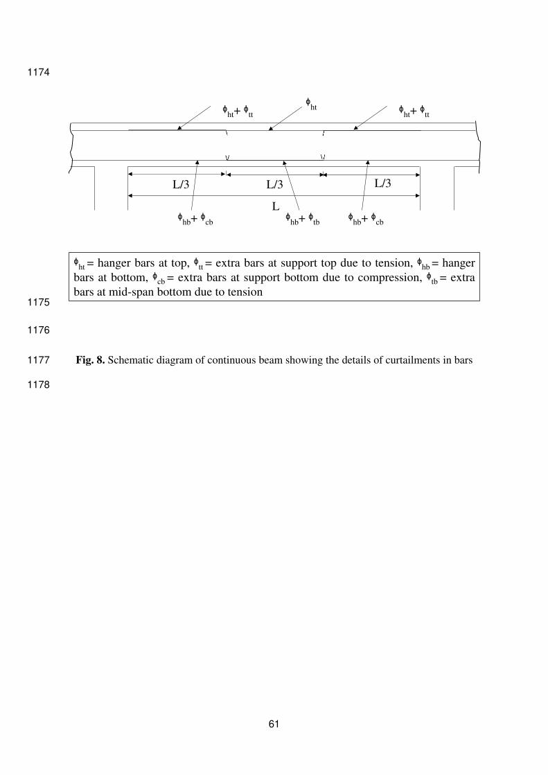
tensile bars in beam has been considered in present study (Fig. 8). Development 462

length of reinforcement of beam and columns at the end supports has not been 463

considered. In case of beam, different shear reinforcement spacing has been used 464

for support and mid span as required as all the beams are continuous with fixed 465

supports. Shear reinforcement for support has been designed for maximum shear 466

force of beam, while shear reinforcement at the mid span designed to carry 467

minimum shear. 468

x) Minimum and maximum diameter of main reinforcing bars for beams and 469

columns are 12mm and 32mm. The diameter of tie bar for shear in beams is 2 470

legged 8 mm and for columns are 8 mm. 471

3.3. Optimization parameters 472

1. Beams are optimized starting from bottom floor to top floor. The search space of the 473

beam design optimization has been restricted in such a way that the maximum value 474

of optimization design variables for a particular floor shall be equal to the optimized 475

design values obtained for the beams in the subsequent bottom floor (except for 476

ground floor). The minimum range of the design variables of all beams have been 477

kept same for all floors. 478

2. Columns are optimized starting from top floor to bottom floor. The search space of 479

the column design optimization has been restricted in such a way that the minimum 480

value of optimization design variables for a particular floor shall be equal to the 481

optimized design values obtained for the columns in the subsequent top floor (except 482

21

for topmost floor). The maximum range of the design variables of all beams have 483

been kept same for all floors. 484

3. Individual beam and column design optimization are performed separately for 10 485

numbers of experiments considering maximum iteration and swarm size 50 and 10 486

respectively. The experiment which exhibit minimum cost has been considered as the 487

optimized design for the respective beam and column. 488

4. In case of continuous beams, all spans have been designed considering the maximum 489

design moments and shear for the beam. 490

3.4. Numerical Results 491

3.4.1. L-shaped building frame 492

In this section developed UPSO based algorithm has been used to optimize the RC design of 493

the G+8 L-shaped building frame to have minimum cost. Search space of design variables 494

should be decided appropriately depending on the experience of the designer, as 495

inappropriate choice of search space can lead to large computational effort.Search space of 496

design variables considered in the study in case of beams are: 𝑏 ∈ [200,400], 𝐷 ∈497 [300,600], 𝜑𝑡 ∈ [12,20],𝜑𝑏 ∈ [12,20], 𝑛𝑐𝑠 ∈ [2,5],𝑛𝑐𝑚 ∈ [2,5], 𝑛𝑡𝑠 ∈ [2,5],𝑛𝑡𝑚 ∈ [2,5]. 498

Search space of design variables considered in the study in case of columns are: 𝑏𝑐 ∈499 [250,500],𝐷𝑐 ∈ [250,500], 𝑘𝑥 ∈ [0.5,1.2],𝑘𝑦 ∈ [0.5,1.2], 𝜑𝑚 ∈ [12,25],𝑛 ∈500 [2,4].Convergence curve for total cost for M20, M25, M30, and M35 grades of concrete 501

along with Fe 415 steel have been plotted in Fig. 9(a). Total cost of the building frame is 502

found to be varying within the range [3840101, 4014875] for Fe 415 steel and [3564230, 503

3942723] for Fe 500 steel for different grades of concrete. It can be observed that variation 504

among different grades of concrete is 4.5% and 10.7% for Fe 415 and Fe 500 steel. Next, Fig. 505

9(b) has been plotted showing the convergence curves of the total cost of concrete, total cost 506

formwork and total cost of steel through all the iterations for M20 grade of concrete and 507

Fe415 grade of steel. This will give designers a good insight regarding the inter-relationship 508

among these three parameters. Also, a bar diagram has been presented showing the 509

comparisons of total cost of the frame for different grades of steel (Fe415, Fe500) and 510

concrete (M20, M25, M30, M35) in Fig. 9(c). It can be seen that for all concrete grades, Fe 511

500 steel yields lower cost than Fe415 steel.Optimized design output for beams and columns 512

obtained from the algorithm has been reported respectively in Table 2 and Table 3 for 513

M20concrete and Fe 415 steel. Beam design details of only three floors have been presented 514

22

for brevity (Table 2), whereas typical column design details for all the floors have been 515

presented (Table 3). In case of columns6 mm diameter of links are considered throughout and 516

the spacing is 190mm c/c, 255mm c/c and 300mm c/c for 12 mm, 16 mm, and 20 mm 517

diameter main bars respectively. 518

Thus, the present algorithm has been found to be very flexible and effective to provide cost 519

optimized design for multistoried L shaped building, considering all the codalprovisions (IS 520

456 [40]) and the practical considerations. 521

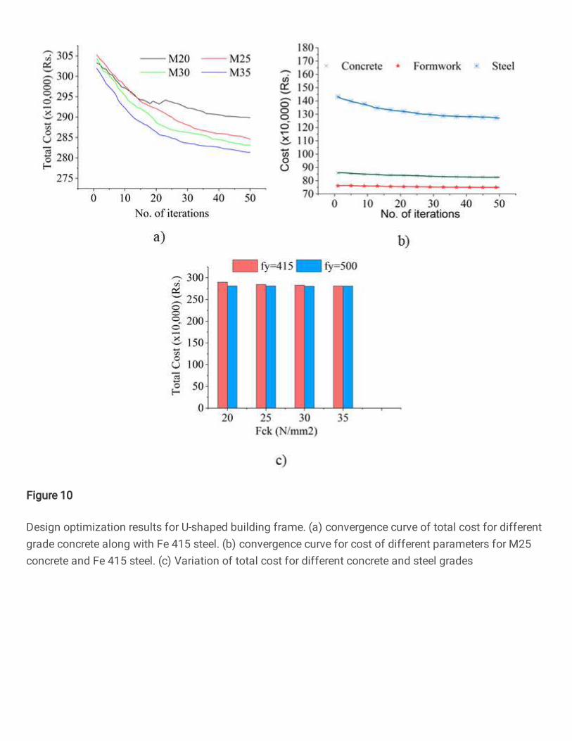
3.4.2. U-shaped building frame 522

In this section developed UPSO based algorithm has been used to optimize the RC design of 523

the G+10 U-shaped building frame to have minimum cost. Search space of design variables 524

should be decided appropriately depending on the experience of the designer, as 525

inappropriate choice of search space can lead to large computational effort. Search space of 526

design variables considered in the study in case of beams are: 𝑏 ∈ [200,250], 𝐷 ∈527 [500,300], 𝜑𝑡 ∈ [12, 16],𝜑𝑏 ∈ [12, 16], 𝑛𝑐𝑠 ∈ [2, 5],𝑛𝑐𝑚 ∈ [2, 5], 𝑛𝑡𝑠 ∈ [2, 5],𝑛𝑡𝑚 ∈ [2, 5]. 528

Search space of design variables considered in the study in case of columns are: 𝑏𝑐 ∈529 [250,400], 𝐷𝑐 ∈ [250,400], 𝑘𝑥 ∈ [0.5,1.2],𝑘𝑦 ∈ [0.5,1.2], 𝜑𝑚 ∈ [12,20],𝑛 ∈530 [2,3].Convergence curve for total cost for M20, M25, M30, and M35 grades of concrete 531

along with Fe 415 steel have been plotted in Fig. 10(a). Total cost of the building frame is 532

found to be varying within the range [2813601, 2898791] for Fe 415 steel and [2805123, 533

2813406] for Fe 500 steelfor different grades of concrete Hence, the maximum variation in 534

total cost among different grades of concrete is found to be 3.03 % and 0.30 % for Fe 415 and 535

Fe 500 steel respectively. Fig. 10(b) representsthe convergence curves of the total cost of 536

concrete, total cost formwork and total cost of steel through all the iterations for M25 grade 537

of concrete and Fe415 grade of steel.A bar diagram showing the total cost of frame was 538

outlined in Fig. 10(c) for various grades of concrete (M20, M25, M30, M35) and steel 539

(Fe415, Fe500). There is not much difference in the cost output for Fe 415 and Fe 500 as 540

observed in the previous problem. It can be seen that for all concrete grades, Fe 500 steel 541

yields lower cost than Fe415 steel. While beam design details of three different floors have 542

been presented in Table 4, column design details has been presented in Table 5 for typical 543

columns in all the floors. M25 concrete and Fe 415 steel are considered for design outputs of 544

both the tables.The diameter and spacing of links in columns are similar to the results 545

reported for L-shaped building frame.The present algorithm is adequately apt, suitably 546

23

adaptable and effectively potent to provide cost optimized design of reinforced concrete 547

buildings U- shaped building frame considering all the codal provisions(IS 456 [40])and 548

practical considerations. 549

3.5. Statistical Analysis 550

As optimization algorithms are based on random processes, possibility of coming up 551

with a different solution is quite common when a large number of experiments are involved. 552

However, the probability of the optimized objective function value to lie within an acceptable 553

range decides the robustness of the optimization algorithm. For that, a large number of 554

experiments are required and each and every solution should be checked whether it is in the 555

acceptable range of the optimum solution. It is a very time consuming and rigorous to 556

conduct a huge number of experiments (i.e. 5000 or 10,000) on the developed algorithm and 557

check every solution manually. In that case, the Monte Carlo simulation (Metropolis and 558

Ulam[53], Metropolis [54]) is used to assess the variations of the solutions of the developed 559

algorithm for large of number of experiments. However, the variations in results should be 560

within an acceptable range for an engineer to accept the results. Monte Carlo simulation is a 561

mathematical numerical method that uses random draws to perform calculations and complex 562

problems. The method was first introduced by Stanislaw Ulam (Eckhardt [55]) and is based 563

on the game of dice, roulette etc. Monte Carlo simulation can be used create large number of 564

solutions of the problem in hand numerically from a small available number of solutions 565

based on a normal distribution curve or bell curve. Then the normal distribution curve can be 566

used to obtain the forecast of the favorable solution and its probability. The probability of the 567

occurrence of the favourable solution among a large number of experiments can be estimated 568

in the normal distribution curve. This decides the robustness of the developed algorithm. 569

In the present study aMonte Carlo simulation for 5000 probable solutions (total cost of 570

frames) of the developed algorithm was performed using MS excel.The expression for 571

probable solution of each simulation was worked out using the following expression in Eq. 572

41. 573

𝑡𝑜𝑡_𝑐𝑜𝑠𝑡𝑖+1 = 𝑡𝑜𝑡_𝑐𝑜𝑠𝑡𝑖 × 𝑒𝐷𝑟+𝑅 , 𝑖 = 1,2, … ,5000 (41)

where, 𝐷𝑟 and 𝑅 can be calculated from Eq. 42 and Eq. 43 respectively. 574

24

𝐷𝑟 = 𝜇𝐸– 𝜎2/2

(42)

𝑅 = 𝜎 × 𝑛𝑜𝑟𝑚𝑠𝑖𝑛𝑣(𝑟𝑎𝑛𝑑(0,1)) (43)

Where, 𝑛𝑜𝑟𝑚𝑠𝑖𝑛𝑣 is an excel function which returns probability corresponding to the 575

standard normal distribution with a mean of zero and a standard deviation of one. 𝜇𝐸 and 𝜎 576

are respectively mean and standard deviation of the 10 number of available total cost values. 577 𝜇𝐸 is considered as 𝑡𝑜𝑡_𝑐𝑜𝑠𝑡𝑖for calculating the values for first simulation. 578

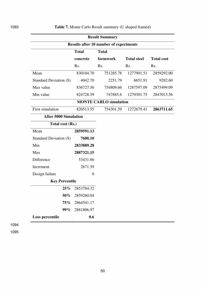
Summary of results of 10 numbers of experiments obtained employing the optimization 579

algorithm along with the key solution of Monte Carlo simulation is presented in Table 6 and 580

Table 7 for L-shaped building frame and U-shaped building frame respectively. Total cost of 581

L-shaped and U-shaped building frame are found to be lying in the ranges of [3792373.03, 582

3923637.97] and [2833889.28, 2887321.15] respectively after 5000 simulations. These 583

ranges are divided into 20 equal divisions. The probability of total cost falling within each 584

interval was estimated considering 5000 forecasted solutions. These probability values 585

obtained for 20 intervals are plotted in Fig. 11 and Fig. 12 for L-shaped and U-shaped frames 586

respectively. Both the plots clearly depict the nature of a normal distribution curve.The most 587

likely solution is at the middle of the curves, meaning there is an equal chance that the actual 588

solutionwill be higher or lower than that value. The key percentile shows the likely values of 589

the total cost of frames.For example, the key percentile value against the 25% shows that 590

there is 25% chance that the developed algorithm will provide this total cost. Similarly, key 591

percentiles for 50% and 75% chance have also been evaluated. Key percentile values are 592

presented in Table 6 and Table 7 for L-shaped and U-shaped building frame 593

respectively.Also, the total cost corresponding to 99% for both the frames also proves that 594

there is negligiblescope for design failure by the developed algorithm. Loss percentile is 595

calculated keeping the maximum total cost to be Rs. 39, 00,000 and Rs. 28, 80,000 for L-596

shaped and U-shaped frame respectively. The loss percentile shows that there is only 2% 597

chance of the total cost to exceed Rs. 39, 00,000 (Table. 6) for L-shaped frame and 0.6% 598

chance to exceed Rs. 28, 80,000 (Table 7) for U-shaped frame, which are very close to first 599

simulation values. The loss percentages are found to be very negligible. Therefore, the 600

optimum design of the frames using the developed algorithm is not only found safe in every 601

experiments but it also provide an optimum overall cost almost every time. 602

25

3.6. Feasibility analysis in terms of safety 603

In the present algorithm beams and columns are optimized separately and added later to 604

obtain the optimized design for the entire frame. Therefore, the stiffness redistribution among 605

beams and columns due to varying sizes of them in each iteration of the optimization have 606

not been taken into account. Thus, from mathematical point of view slight error has been 607

imparted into the analysis. In the present algorithm a few measures have been taken to ensure 608

the safety of the structures. The analysis and preliminary design of the buildings are 609

performed in STAAD Pro, in such way that sizes of all beams and columns has been chosen 610

in a conservative manner. It was then made sure that design was safe as per design standard. 611

Next, design forces (shear force, moment and axial forces) have been taken from the 612

conservative STAAD Pro model and fed into the developed optimization algorithm in 613

MATLAB. In that way the sizes of beams and columns only reduced during optimization 614

procedure as can be seen from Table 2-5. The design force is kept same as the preliminary 615

analysis of STAAD Pro. In that way, it has been made sure that design was always carried 616

out for design forces higher than the actual design forces obtained during the course of the 617

optimization program. After optimization is done, optimized member sizes are incorporated 618

in STAADPro model to compare the design forces of optimized structures with actual 619

STAADPro model. Table 8-9 have been presented showing the comparison between the 620

design forces of the structures before and after optimization for a typical fourth floor of one 621

building (L-shaped). Actual design forces and moments of optimized structure are observed 622

to be significantly lower than the design forces and moments of the structure before 623

optimization. So, the optimized design has been indeed carried out for higher design forces 624

and moments than the actual. Therefore, the aforementioned error has not influence the safety 625

of the buildings significantly enough to violate the safety criteria provided by the design 626

standard. So, from practical civil engineering point of view the design results obtained from 627

present algorithm is feasible and safe enough to be used for cost-optimum design of RC 628

building frame. 629

4.Conclusion 630

In the present study, an UPSO based optimization algorithm has been developed in 631

MATLAB [56]environment to find cost optimum design of reinforcement concrete building 632

frame considering the codal specifications of safety and serviceability of IS 456 [33] along 633

with the consideration for the construction requirements in practical field. 634

26

Two building frames namely G+8 L-shaped frame and G+10 U-shaped frame have been 635

adopted to demonstrate the efficacy of the developed algorithm. Popular design and analysis 636

software STAADPro. V8i [52] has been used to obtain the design forces (bending moments, 637

shear forces and axial forces) in critical sections of all the beams and columns considering the 638

effects of gravity loads, wind loads and seismic loads as per the specifications of the 639

respective Indian Standards. Next, each beam and column are optimized separately 640

employing UPSO based algorithm. Thus, total optimized cost of the frames hasbeen obtained 641

by adding up all the optimized costs of these beams and columns. Numerical results have 642

revealed that the present algorithm is capable of providing cost optimized design of RC 643

frames of any shape and height with profound accuracy.Further, Monte Carlo 644

simulationperformed assures the consistency and robustness of the developed algorithm with 645

almost hundred percent design success. This further confirms that the algorithm can be 646

effectively used for optimal design of any type of reinforced concrete buildings having 647

different design constraints. Only the design variables and constraints need to be modified to 648

adapt to the particular building problem. Overall, the present UPSO based algorithm has been 649

found to be very effective in finding cost optimum design of RC frame having any planner 650

irregularity and any number of floors.The positive findings of the research will encourage the 651

future researchers to improve the present algorithm to incorporate more minute reinforcement 652

details such as development length, ductile detailing etc.Also, finite element method can be 653

incorporated within the algorithm to obtain the design forces directly instead of relying on 654

commercial design software. In that way accuracy of the results can be improved further. 655

656

Data availability statement 657

All the required data presented in the manuscript itself. Any further dataimportant to the 658

readers can be made available as per their request. 659

Acknowledgement 660

The author wish to acknowledge anonymous reviewers for their valuable suggestions and 661

comments. The authors are grateful to department of Civil Engineering, IIT Kharagpur to 662

provide the necessary infrastructure to carry out the research work. 663

Conflict of interest 664

27

On behalf of all authors, the corresponding author states that there is no conflict of interest. 665

Replication of results 666

The authors hereby statethat they are willing to share all the codes and numerical data needed 667

to reproduce the figures. 668

669

28

References 670

[1] Milajić, A., Pejicic, G., and Beljakovic, D. (2013). “Optimal Structural Design of 671

Reinforced Concrete Structures – Review of Existing Solutions.” Archives for 672

Technical Sciences, 9(1), 53–60. 673

[2] Hasencebi, O., Teke, T., and Pekcan, O. (2013). “A bat-inspired algorithm for 674

structural optimization.” Computers and Structures, 128, 77-90. 675

[3] Wang, L., Zhang, H. and Zhu, M. (2020). “A new Evolutionary 676

StructuralOptimization method and application for aided design to reinforced 677

concretecomponents.” Struct Multidisc Optim. https://doi.org/10.1007/s00158-020-678

02626-z. 679

[4] Lu, H., Gilbert, M. and Tyas, A. (2019). “Layout optimization of building frames 680

subject to gravity and lateral load cases”. Struct Multidisc Optim 60, 1561–1570. 681

[5] Lee, J. (2019). “Multi-objective optimization case study with active and passive 682

design in building engineering.” Struct Multidisc Optim 59, 507–519. 683

[6] Zegard, T., Hartz, C., Mazurek, A. (2020). “Advancing building engineering through 684

structural and topology optimization.” Struct Multidisc Optim. 685

https://doi.org/10.1007/s00158-020-02506-6. 686

[7] Prakash, A., Agarwala, S. K., and Singh, K. K. (1988). “Optimum design of 687

reinforced concrete sections.” Computers and Structures, 30(4), 1009–1011. 688

[8] Chakrabarty, B. K. (1992). “Models for optimal design of reinforced concrete 689

beams.” Computers and Structures, 42(3), 447–451. 690

[9] Coello, C. C., Hernández, F. S., and Farrera, F. A. (1997). “Optimal design of 691

reinforced concrete beams using genetic algorithms.” Expert Systems with 692

Applications, 12(1), 101–108. 693

[10] Rajeev, S., and Krishnamoorthy, C. S. (1998). “Genetic algorithm-based 694

methodology for design optimization of reinforced concrete frames.” Computer-695

Aided Civil and Infrastructure Engineering, 13(1), 63–74. 696

29

[11] Dole, M. R., Ronghe, G. N., and Gupta, L. M. (2000). “Optimum design of 697

reinforced concrete beams using polynomial optimization technique.” Advances in 698

Structural Engineering, 3(1), 67–79. 699

[12] De Medeiros, G. F., and Kripka, M. (2013). “Structural optimization and 700

proposition of pre-sizing parameters for beams in reinforced concrete buildings.” 701

Computers and Concrete, 11(3), 253–270. 702

[13] Nigdeli, S. M., and Bekdaş, G. (2017). “Optimum design of RC continuous beams 703

considering unfavourable live-load distributions.” KSCE Journal of Civil 704

Engineering, 21(4), 1410–1416. 705

[14] Uz, M. E., Sharafi, P., Askarian, M., Fu, W., and Zhang, C. (2018). “Automated 706

layout design of multi-span reinforced concrete beams using charged system search 707

algorithm.” Engineering Computations, 35(3), 1402–1413. 708

[15] Ferreira, C. C., Barros, M. H. F. M., and Barros, A. F. M. (2003). “Optimal design 709

of reinforced concrete T-sections in bending.” Engineering Structures, 25(7), 951–710

964. 711

[16] Preethi, G., and Arulraj, P. G. (2016). “Optimal Design of Axially Loaded RC 712

Columns.” Bonfring International Journal of Industrial Engineering and 713

Management Science, 6(3), 78–81. 714

[17] Bekdaş, G., and Niğdeli, S. M. (2016). “Optimum design of reinforced concrete 715

columns employing teaching-learning based optimization.” Challenge Journal of 716

Structural Mechanics, 2(4), 216–219. 717

[18] Aldwaik, M. and Adeli, H. (2016). “Cost optimization of reinforced concrete flat 718

slabsof arbitrary configuration in irregular highrise building structures.” Struct 719

MultidiscOptim54, 151–164. 720

[19] Aldwaik, M. and Adeli, H. (2014). “Advances in optimization of 721

highrisebuildingstructures.” Struct Multidisc Optim50, 899–919. 722

[20] Chaudhuri, P. and Maity, D. (2020).“Cost optimization of rectangular RC footing 723

using GA and UPSO.” Soft Computing, 24 (January), 709–721 724

30

[21] Kaveh, A., and Behnam, A. F. (2013). “Design optimization of reinforced concrete 725

3D structures considering frequency constraints via a charged system search.” 726

ScientiaIranica, Elsevier B.V., 20(3), 387–396. 727

[22] Bekdaş, G., and Nigdel, S. M. (2014). “Optimization of RC frame structures 728

subjected to static loading.” 11th World Congress on Computational Mechanics, 729

WCCM 2014, 5th European Conference on Computational Mechanics, ECCM 730

2014 and 6th European Conference on Computational Fluid Dynamics, ECFD 731

2014, (Wccm Xi), 3869–3875. 732

[23] Aga, A. A. A., and Adam, F. M. (2015). “Design Optimization of Reinforced 733

Concrete Frames.” Open Journal of Civil Engineering, 05(01), 74–83. 734

[24] Gharehbaghi, S., and Khatibinia, M. (2015). “Optimal seismic design of reinforced 735

concrete structures under time- history earthquake loads using an intelligent hybrid 736

algorithm.” Earthquake Engineering and Engineering Vibration, 14(1), 97–109. 737

[25] Esfandiary, M. J., Sheikholarefin, S., and Bondarabadi, H. A. R. (2016). “A 738

combination of particle swarm optimization and multi-criterion decision-making 739

for optimum design of reinforced concrete frames.” International Journal of 740

Optimization in Civil Engineering, 6(2), 245–268. 741

[26] Kulkarni, A., and Bhusare, V. (2017). “Structural optimization of reinforced 742

concrete structures Structural Optimization of Reinforced Concrete Structures.” 743

International Journal of Engineering Research & Technology (IJERT), 5(March), 744

123–127. 745

[27] Bekas, G. K., and Stavroulakis, G. E. (2017). “Machine Learning and Optimality in 746

Multi Storey Reinforced Concrete Frames.” Infrastructures, 2(2), 6. 747

[28] Tapao, A., and Cheerarot, R. (2017). “Optimal parameters and performance of 748

artificial bee colony algorithm for minimum cost design of reinforced concrete 749

frames.” Engineering Structures, Elsevier Ltd, 151, 802–820. 750

[29] Esfandiari, M. J., Urgessa, G. S., Sheikholarefin, S., and Manshadi, S. H. D. (2018). 751

“Optimum design of 3D reinforced concrete frames using DMPSO algorithm.” 752

Advances in Engineering Software, 115(September 2017), 149–160. 753

31

[30] RazmaraShooli, A., Vosoughi, A.R. and Banan, M.R. (2019). “A mixed GA-PSO-754

based approach for performance-based design optimization of 2D reinforced 755

concrete special moment-resisting frames.” Applied Soft Computing Journal, 756

85(105843). 757

[31] Milajić, A., Beljakovic, D., and Culic, N. (2014). “Optimal Structural Design Based 758

on Applicability in Practice.” In conference proceedings of People, People, 759

Buildings and Environment, Kroměříž, Czech Republic, 306–315. 760

[32] Milajić, A., Prokic, A., Beljakovic, D., and Pejicic, G. (2015). “Quantitative method 761

for evaluating applicability of designed reinforcement pattern.” 762

Kvantitativnimetodzaocjenuprimjenljivostiprojektiraneshemearmiranja, 22(1), 763

119–124. 764

[33] Nanda, B., Maity, D., Maiti, D.K. (2014). “Modal parameter based inverse 765

approach for structural joint damage assessment using unified particle swarm 766

optimization.”Applied Mathematics and Computation, 242(1), 407-422. 767

[34] Nanda, B., Maity, D., Maiti, D.K. (2014). “Damage assessment from curvature 768

mode shape using unified particle swarm optimization.” Structural Engineering 769

and Mechanics Volume, 52(2), 307-322. 770

[35] Mohan, S. C., Maiti, D. K and Maity, D. (2013) “Structural damage assessment 771

using FRF employing particle swarm optimization” Applied Mathematics and 772

Computation, 219 (20), 10387-10400. 773

[36] Barman S.K., Maiti D.K., Maity D. (2020) Damage Detection of Truss Employing 774

Swarm-Based Optimization Techniques: A Comparison. In: Venkata Rao R., Taler 775

J. (eds) Advanced Engineering Optimization Through Intelligent Techniques. 776

Advances in Intelligent Systems and Computing, 949.21-37 Springer, Singapore. 777

[37] Barman, S. K., Jebieshia, T. R., Tiwari, P, Maiti, D.K. and Maity, D. (2019) “Two-778

Stage Inverse Method to Detect Delamination in Composite Beam Using Vibration 779

Responses” AIAA Journal. 57 (3). 1312-1322. 780

[38] Mishra, M., Barman, S. K, Maity, D and Maiti, D. K. (2020). “Performance 781

Studies of 10 Metaheuristic Techniques in Determination of Damages for Large-782

32

Scale Spatial Trusses from Changes in Vibration Responses.” Journal of 783

Computing in Civil Engineering, 34 (2), 04019052. 784

[39] Parsopoulos, K.E., Kariotou, F., Dassios, G. and Vrahatis, M.N. (2009). ‘Tackling 785

magnetoencephalography with particle swarm optimization’. International Journal 786

of Bio-Inspired Computation, 1(1–2), 32-49 787

[40] IS 456 (2000). Plain and Reinforced Concrete - Code of Practice, Bureau of Indian 788

Standards, New Delhi, India 789

[41] IS 875 (Part I) (1987). Code of practice for design loads (other than earthquake)for 790

buildings and structures: part 1 dead loads - unit weights of building material and 791

stored materials, Bureau of Indian Standards, New Delhi, India 792

[42] IS 875 (Part II) (1987). Code of practice for design loads (other than earthquake) 793

for buildings and structures: part 2 imposed loads, Bureau of Indian Standards, 794

New Delhi, India 795

[43] SP 64 (Part III) (2001). Explanatory handbook on Indian standard code of practice 796

for design loads (other than earthquake) for buildings and structures, Bureau of 797

Indian Standards, New Delhi, India 798

[44] IS 875 (Part III) (2015). Design loads (other than earthquake) for buildings and 799

structures - code of practice - part 3 wind loads, Bureau of Indian Standards, New 800

Delhi, India 801

[45] IS 1893 (Part I) (2016). Criteria for earthquake resistant design of structures - part 802

1: general provisions and buildings, Bureau of Indian Standards, New Delhi, India 803

[46] IS 875 (Part V) (2015). Code of practice for design loads (other than 804

earthquake)for buildings and structures: part 5special loads and load 805

combinations, Bureau of Indian Standards, New Delhi, India 806

[47] Parsopoulos, K. E., and Vrahatis, M. N. (2005). “Unified Particle Swarm 807

Optimization for Solving Constrained Engineering Optimization Problems.” 808

Advances in natural computation, Springer, Springer Berlin Heidelberg, Berlin, 809

Heidelberg, 582–591. 810

33

[48] Kennedy, J. and Eberhert, R. (1995). “Particle swarm optimization.” International 811

Conference on Neural Networks, IEEE, Australia. 812

[49] Perez, R. E., and Behdinan, K. (2007). “Particle swarm approach for structural 813

design optimization.” Computers and Structures, 85(19), 1579-1588. 814

[50] Parsopoulos, K. E., and Vrahatis, M. N. (2010).Particle Swarm Optimization and 815

Intelligence, Vol. 270, 2010. doi:10.4018/978-1-61520-666-7. 816

[51] WB PWD schedule.(2017) Schedule of rates, volume I: building works. Public 817

Works Department (PWD), Government of West Bengal (WB), India 818

[52] STAAD Pro V8i (2017). Select series 6, Bentley Systems, Inc. PA, USA. 819

[53] Metropolis, N., andUlam, S. (1949). “The Monte Carlo Method.”Journal of the 820

American Statistical Association, 44(247), 335-341. doi:10.2307/2280232 821

[54] Metropolis, N. (1987). The beginning of the Monte Carlo method. Los Alamos 822

Science15: 125-130 823

[55] Eckhardt, R. (1987). “Stan Ulam, John Von Neumann, and the Monte Carlo 824

method.” Los Alamos Science, 15, 131--136. 825

[56] MATLAB (2015), TheMathworks Inc. USA. 826

827

34

APPENDIX I. Notation 828

The following symbols have been used in this paper: 829

𝐴ℎ = Horizontal acceleration coefficient 830

𝑊 = Seismic weight of building 831

𝑍 = Seismic zone factor 832

𝑆𝑎𝑔 = Design acceleration coefficient 833

𝑇𝑎 = Natural period of building 834

𝐻𝑏𝑙= Height of the building from plinth level 835 𝐷𝑏𝑙 = Base dimension of the building in the direction of earthquake 836

shaking 837

𝑅 = Response reduction factor 838

𝐼 = Importance factor 839

𝑝𝑑 = Design wind pressure 840

𝐾𝑑 = Wind directionality factor 841

𝐾𝑎 = Area averaging factor 842

𝐾𝑐 = Combination factor 843

𝑉𝑧 = Design wind speed 844

𝑉𝑏 = Basic wind speed 845

𝑘1 = Probability factor 846

𝑘2 = Terrain roughness and height factor 847

𝑘3 = Topology factor 848

35

𝑘4 = Importance factor for cyclonic region 849

𝑏 = Width of the beam 850

𝐷 = Overall depth of the beam 851

𝑑𝑒 = Effective depth of the beam 852

𝑑′= depth of compression reinforcement from compression face of 853

beam. 854 𝑙𝑐= effective length of column 855 𝐷𝑐= width/ depth of the column 856

𝑥𝑢𝑚𝑎𝑥𝑑𝑒 = Limiting neutral axis depth factor for beam. 857

𝑓𝑐𝑘 = Grade of concrete 858

𝑓𝑦 = Grade of steel reinforcement 859

𝐴𝑠𝑡 = Area of tensile reinforcement for beam 860

𝐴𝑠𝑐 = Area of compressive reinforcement for beam 861

𝜏𝑣 = Nominal shear strength 862

𝜏𝑐 = Shear strength of concrete 863

𝜏𝑐𝑚𝑎𝑥 = Maximum shear strength of concrete 864

𝑠𝑣 = Spacing of shear reinforcement for beam 865

𝐴𝑠𝑣 = Total cross sectional area of the stirrup legs 866

𝑎𝑠 = Short term deflection of beam 867

𝑎𝑐𝑠 = Deflection of beam due to shrinkage 868

𝑎𝑐𝑐 = Deflection of beam due to creep 869

36

𝐸𝑐 = Short term elasticity modulus for beam 870

𝐼𝑒𝑓𝑓 = Effective moment of inertia for short term deflection of beam 871

𝐼𝑟 = Moment of inertia of cracked section of beam 872

𝐼𝑔𝑟 = Gross moment of inertia of beam 873

𝑀𝑟 =Cracking moment 874

𝑓𝑐𝑟 = Modulus of rupture of concrete 875 𝑦𝑡 = Distance from the centroidal axis of gross section, neglecting the 876

reinforcement, to extreme fibre in tension 877 𝑀 = Maximum moment under service load for beam 878 𝑧 = Lever arm of the beam section 879 𝑥 = Depth of the neutral axis for beam 880 𝑏𝑤 = Breadth of web for beam 881 𝑏𝑏 = Breadth of compression face for beam 882 𝑓3 = Constant depending upon the support condition of beam 883 𝜑𝑐𝑠 = Shrinkage curvature for beam 884 𝑓4 = Factor depending on percentage of tensile and compressive 885

reinforcement for beam 886 ∈𝑐𝑠= Ultimate shrinkage strain of concrete for beam 887 𝑙 = Length of the span of beam 888 𝑎𝑖,𝑐𝑐 = Initial plus creep deflection of beam due to permanent loads 889

𝐸𝑐𝑒 = Young’s modulus of concrete to calculate 𝑎𝑖,𝑐𝑐 890

37

𝐸𝑐= Actual Young’s modulus of concrete to calculate short term 891

deflection 892 𝜃= Creep coefficient 893 𝐷𝑐 =Depth of the column 894 bc =width of column 895 𝑙𝑐 =Length of the column. 896 Ac = Area of the concrete in column section 897 Ascc = Area of reinforcement in column 898 𝜑𝑚= Diameter of the main bar of the column 899 iter = number of iterations in each experiment for the developed 900

MATLAB program. 901 𝑚𝑎x_iter = maximum number of iterations in each experiment for the 902

developed MATLAB program. 903 𝑒𝑥𝑝 = number of experiments, i.e., 1,2,3,…. 904 𝑛𝑒𝑥𝑝 = maximum number of experiments considered. 905 𝑉𝑐= Volume of gross concrete work of beam / column in cubic meters. 906 𝑉𝑠=Volumeof steel reinforcement of beam / column in cubic meters. 907 𝜌𝑠= Density of steel i.e. 7850 Kg/m3. 908 𝐶𝑐= Cost of reinforced concrete work per cubic meters. 909 𝐶𝑠= Cost of steel reinforcement per Kg. 910 𝐶𝑓= Cost of formwork per square meters. 911

912

38

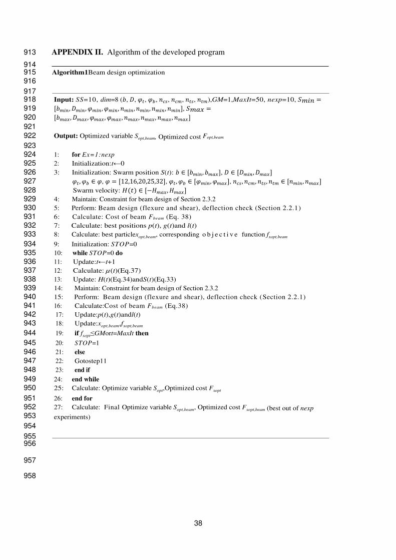
APPENDIX II. Algorithm of the developed program 913

914 Algorithm1Beam design optimization 915

916

917 Input: SS=10, dim=8 (𝑏, 𝐷, 𝜑𝑡, 𝜑𝑏, 𝑛𝑐𝑠, 𝑛𝑐𝑚, 𝑛𝑡𝑠, 𝑛𝑡𝑚),GM=1,MaxIt=50, nexp=10, 𝑆𝑚𝑖𝑛 =918 [𝑏𝑚𝑖𝑛, 𝐷𝑚𝑖𝑛, 𝜑𝑚𝑖𝑛, 𝜑𝑚𝑖𝑛, 𝑛𝑚𝑖𝑛, 𝑛𝑚𝑖𝑛, 𝑛𝑚𝑖𝑛, 𝑛𝑚𝑖𝑛], 𝑆𝑚𝑎𝑥 =919 [𝑏𝑚𝑎𝑥, 𝐷𝑚𝑎𝑥, 𝜑𝑚𝑎𝑥 , 𝜑𝑚𝑎𝑥, 𝑛𝑚𝑎𝑥, 𝑛𝑚𝑎𝑥, 𝑛𝑚𝑎𝑥, 𝑛𝑚𝑎𝑥] 920

921

Output: Optimized variable Sopt,beam, Optimized cost Fopt,beam 922

923

1: for Ex=1:nexp 924

2: Initialization:t←0 925

3: Initialization: Swarm position S(t): 𝑏 ∈ [𝑏𝑚𝑖𝑛, 𝑏𝑚𝑎𝑥], 𝐷 ∈ [𝐷𝑚𝑖𝑛, 𝐷𝑚𝑎𝑥] 926

𝜑𝑡 , 𝜑𝑏 ∈ 𝜑, 𝜑 = [12,16,20,25,32], 𝜑𝑡 , 𝜑𝑏 ∈ [𝜑𝑚𝑖𝑛, 𝜑𝑚𝑎𝑥], 𝑛𝑐𝑠, 𝑛𝑐𝑚, 𝑛𝑡𝑠, 𝑛𝑡𝑚 ∈ [𝑛𝑚𝑖𝑛, 𝑛𝑚𝑎𝑥] 927

Swarm velocity: 𝐻(𝑡) ∈ [−𝐻𝑚𝑎𝑥, 𝐻𝑚𝑎𝑥] 928

4: Maintain: Constraint for beam design of Section 2.3.2 929

5: Perform: Beam design (flexure and shear), deflection check (Section 2.2.1) 930

6: Calculate: Cost of beam Fbeam (Eq. 38) 931

7: Calculate: best positions p(t), g(t)and l(t) 932

8: Calculate: best particlexopt,beam, corresponding o b j e c t i v e function fxopt,beam 933

9: Initialization: STOP=0 934

10: while STOP=0 do 935

11: Update:t←t+1 936

12: Calculate: µ(t)(Eq.37) 937

13: Update: H(t)(Eq.34)andS(t)(Eq.33) 938

14: Maintain: Constraint for beam design of Section 2.3.2 939

15: Perform: Beam design (flexure and shear), deflection check (Section 2.2.1) 940

16: Calculate:Cost of beam Fbeam (Eq.38) 941

17: Update:p(t),g(t)andl(t) 942

18: Update:xopt,beam,fxopt,beam 943

19: if fxopt≤GMort=MaxIt then 944

20: STOP=1 945

21: else 946

22: Gotostep11 947

23: end if 948

24: end while 949

25: Calculate: Optimize variable Sopt,Optimized cost Fxopt 950

26: end for 951

27: Calculate: Final Optimize variable Sopt,beam, Optimized cost Fxopt,beam (best out of nexp 952

experiments) 953

954

955 956

957

958

39

959 Algorithm2 Column design optimization 960

961 962

Input: SS=10, dim= 6 (𝑏𝑐, 𝐷𝑐, 𝑘𝑥, 𝑘𝑦, 𝜑𝑚, 𝑛),GM=1,MaxIt=50, nexp=10, 𝑆𝑚𝑖𝑛 =963 [𝑏𝑐,𝑚𝑖𝑛, 𝐷𝑐,𝑚𝑖𝑛, 𝑘𝑥,𝑚𝑖𝑛, 𝑘𝑦,𝑚𝑖𝑛, 𝜑𝑚𝑖𝑛, 𝑛𝑚𝑖𝑛], 𝑆𝑚𝑎𝑥 = [𝑏𝑐,𝑚𝑎𝑥, 𝐷𝑐,𝑚𝑎𝑥, 𝑘𝑥,𝑚𝑎𝑥, 𝑘𝑦,𝑚𝑎𝑥, 𝜑𝑚𝑎𝑥, 𝑛𝑚𝑎𝑥] 964

965

Output: Optimized variable Sopt,column, Optimized cost Fopt,column 966

967

1: for Ex=1:nexp 968

2: Initialization:t←0 969

3: Initialization:SwarmpositionS(t): 970

𝑏𝑐 ∈ [𝑏𝑐,𝑚𝑖𝑛, 𝑏𝑐,𝑚𝑎𝑥], 𝐷𝑐 ∈ [𝐷𝑐,𝑚𝑖𝑛, 𝐷𝑐,𝑚𝑎𝑥], 𝑘𝑥 ∈ [𝑘𝑥,𝑚𝑖𝑛, 𝑘𝑥,𝑚𝑎𝑥], 𝑘𝑦 ∈ [𝑘𝑦,𝑚𝑖𝑛, 𝑘𝑦,𝑚𝑎𝑥] 971

𝜑𝑚 ∈ 𝜑, 𝜑 = [12,16,20,25,32], 𝜑𝑚 ∈ [𝜑𝑚𝑖𝑛, 𝜑𝑚𝑎𝑥], 𝑛 ∈ [𝑛𝑚𝑖𝑛, 𝑛𝑚𝑎𝑥] 972

973

Swarm velocity𝐻(𝑡) ∈ [−𝐻𝑚𝑎𝑥, 𝐻𝑚𝑎𝑥] 974

4: Maintain: Constraint for column design of Section 2.3.2 975

5: Perform: Column design for longitudinal reinforcement and lateral ties (Section 2.2.2) 976

6: Calculate: Cost of column Fcolumn (Eq.38) 977

7: Calculate: best positions p(t), g(t)and l(t) 978

8: Calculate: best particle xopt,column, corresponding o b j e c t i v e function fxopt,column 979

9: Initialization: STOP=0 980

10: while STOP=0 do 981

11: Update: t←t+1 982

12: Calculate: µ(t) (Eq.37) 983

13: Update: H(t) (Eq.34) and S(t) (Eq.33) 984

14: Maintain: Constraint for column design of Section 2.3.2 985

15: Perform: Column design for longitudinal reinforcement and lateral ties (Section 2.2.2) 986

16: Calculate: Cost of column Fcolumn (Eq.38) 987

17: Update: p(t),g(t)andl(t) 988

18: Update: xopt,column, fxopt,column 989

19: if fxopt ≤ GMort=MaxIt then 990

20: STOP=1 991

21: else 992

22: Gotostep11 993

23: end if 994

24: end while 995

25: Calculate: Optimize variable Sopt, Optimized cost Fxopt 996

26: end for 997

27: Calculate: Final Optimize variable Sopt,column, Optimized cost Fxopt,column (best out of nexp 998

experiments) 999

1000 1001

1002

1003

1004

1005

40

1006 Algorithm3 Combined optimized cost of frame 1007

1008 1009

Input:𝑋𝑚𝑖𝑛,𝑋𝑚𝑎𝑥 (as per Section.3.4), Design forces: Moment and shear force for beams, 1010

Axial forces and biaxial moments for columns from STAAD 1011

1012

Output: Optimized designs:Xopt,beam, Xopt,column, Optimized cost: Fopt,beam, Fopt,column 1013

1014 1: Beam design optimization (Algorithm 1): One by one from ground floor to top floor. Update 1015 𝑋𝑚𝑖𝑛,𝑋𝑚𝑎𝑥 for each floor (Section 3.3). 1016

2: Column design optimization (Algorithm 2): One by one from top floor to ground floor. Update 1017 𝑋𝑚𝑖𝑛,𝑋𝑚𝑎𝑥 for each floor (Section 3.3). 1018

3: Find out optimum beam design and column design 1019

3: Calculate total optimize cost of frame=∑ 𝐹𝑜𝑝𝑡,𝑏𝑒𝑎𝑚 + ∑ 𝐹𝑜𝑝𝑡,𝑐𝑜𝑙𝑢𝑚𝑛 1020

1021 1022

1023 1024

41

APPENDIX III 1025

1026

Parameters used in design of beam: 1027

For doubly reinforced beam 1028

Table I Stress in compression reinforcement (𝑓𝑠𝑐), (N/mm2) in doubly reinforced beams with cold 1029 worked bars 1030

SP16 Table F 𝑑′/𝑑 𝑓𝑦 =415 N/mm2 𝑓𝑦 =500 N/mm2

0.05 355 424

0.1 353 412

0.15 342 395

0.2 329 370

1031

For design of beam in shear 1032

Design shear strength 𝜏𝑐 = 0.85√0.8𝑓𝑐𝑘(√1+5𝛽−1)6𝛽 , 𝛽 = 0.8𝑓𝑐𝑘6.89𝑃𝑡 ≥ 1, 𝑃𝑡 = 100𝐴𝑠𝑡𝑏𝑑 , 𝐴𝑠𝑡 is area of tensile reinforcement, 1033 𝑏, 𝑑 are width and effective depth.𝑓𝑐𝑘= Grade of concrete 1034

1035

Table II Maximum Shear Stress (𝜏𝑐,𝑚𝑎𝑥), N/mm2 (IS 456) 1036

Table 24 (Clauses B-2.3, B-5.2.3. B·5.2.3. t, B.5.5,1 and B-

6.3.1) 𝑓𝑐𝑘 (N/mm2) 15 20 25 30 35 40 𝜏𝑐,𝑚𝑎𝑥(N/mm2) 2.5 2.8 3.1 3.5 3.7 4

1037

For deflection check in beam 1038 𝑓3 =0.5 for cantilevers, 0.125 for simply supported members, 0.086 for continuous at one end and 0.063 for fully 1039

continuous members 1040 𝑓4 = 0.72 𝑃𝑡−𝑃𝑐√𝑃𝑡 ≤ 1.0 for0.25 ≤ 𝑃𝑡 − 𝑃𝑐 ≤ 1.0 1041 = 0.65 𝑃𝑡−𝑃𝑐√𝑃𝑡 ≤ 1.0 for 𝑃𝑡 − 𝑃𝑐 ≥ 1.0, 𝑃𝑡 = 100𝐴𝑠𝑡𝑏𝑑 , 𝑃𝑐 = 100𝐴𝑠𝑐𝑏𝑑 , 𝐴𝑠𝑐 is area of compressive reinforcement. 1042

1043

Parameters used in design of column: 1044

1045

Table III Salient points on the design stress-strain curve for cold-worked bars 1046

SP 16 (Table A) 𝑓𝑦 =415 N/mm2 𝑓𝑦=500 N/mm2

Strain Stress (N/mm2) Strain Stress (N/mm2)

0.00144 288.7 0.00174 347.8

0.00163 306.7 0.00195 369.6

0.00192 324.8 0.00226 391.3

0.00241 342.8 0.00277 413

0.00276 351.8 0.00312 423.9

0.0038 360.9 0.00417 434.8

1047

42

1048

Parameters used in wind analysis: 1049

1050 Table IV Risk coefficient (𝑘1) for structures in different wind speed zones 1051

1052

IS 875 part 3 2015 Table 1 (Clause 6.3.1)

Class of structures Design life of

structures (years)

𝑘1 factor for basic wind speed (m/s)

33 39 44 47 50 55

All general structures 50 1.00 1.00 1.00 1.00 1.00 1.00

Temporary structures 5 0.82 0.76 0.73 0.71 0.70 0.67

Structures with low degree

of hazards 25 0.94 0.92 0.91 0.90 0.90 0.89

Important building 100 1.05 1.06 1.07 1.07 1.08 1.08

1053 1054 Table V Factors to obtain design wind speed variation with height in different terrains (𝑘2) 1055

IS 875 part 3 2015 Table 2 (Clause 6.3.2.2.)

Height

(m) Height multiplier (𝑘2) for terrain

categoty

1 2 3 4

10 1.05 1.00 0.91 0.80

15 1.09 1.05 0.97 0.80

20 1.12 1.07 1.01 0.80

30 1.15 1.12 1.06 0.97

50 1.2 1.17 1.12 1.1

100 1.26 1.24 1.2 1.2

150 1.3 1.28 1.24 1.24

200 1.32 1.3 1.27 1.27

250 1.34 1.32 1.29 1.28

300 1.35 1.34 1.31 1.3

350 1.35 1.35 1.32 1.31

400 1.35 1.35 1.34 1.32

450 1.35 1.35 1.35 1.33

500 1.35 1.35 1.35 1.34

1056

1057

43

List of Tables 1058

1 Review of all the optimization techniques used by the researchers for solving 1059

design optimization problem of RC structures………………………………… 44 1060

2 Beam design details for three different floors - L shaped building frame….........45 1061

3 Typical column design details for all floor - L shaped building frame.………….46 1062

4 Beam design details for three different floors- U shaped building frame.....…….47 1063

5 Typical column design details for all floor –U shaped building frame……..........48 1064

6 Monte Carlo Result summary (L shaped frame)…………………………….…...49 1065

7 Monte Carlo Result summary (U shaped frame)………..………….…………….50 1066

8 MATLAB and STAADPro comparison of beam design (L shaped 1067

frame)…………………………………………………………………………….51 1068

9 MATLAB and STAADPro comparison of column design (L shaped 1069

frame)…………………………………………………………………………….52 1070

10 MATLAB and STAADPro comparison of beam design (U shaped 1071

frame)…………………………………………………………………………….53 1072

11 MATLAB and STAADPro comparison of column design (U shaped 1073

frame)…………………………………………………………………………….54 1074

1075

1076

44

Table 1. Review of all the optimization techniques used by the researchers for 1077

solving design optimization problem of RC structures 1078

Authors Optimization algorithm

Prakash et al.[7] Simplex and Lagrangian optimization

method

Chakrabarty [8] Geometric programming

Coello et al.[9], Rajeev and

Krishnamoorthy[10], Chaudhuri and Maity[20]

Genetic algorithm (GA)

Dole et al. [11] polynomial optimization technique

De Medeiros et al. [12] Simulated annealing (SA)

Nigdeli and Bekdaş [13] random search technique (RST)

Uz et al. [14], Kaveh and Behnam [21] charged system search (CSS)

Preethi and Arulraj [16] sequential quadratic programming (SQP)

Bekdaş and Niğdeli [17] Teaching-learning-based-optimization

(TLBO)

Bekdaş and Nigdel[22] Harmony search (HS)

Aga and Adam[23] Artificial neural network (ANN)

Gharehbaghi and Khatibinia[24] intelligent regression model (IRM)

combined with Particle swarm optimization

(PSO)

Esfandiary et al. [25, 29] decision-making Particle Swarm

Optimization (DMPSO)

Kulkarni and Bhusare[26] Response Surface Method (RSM)

Tapao and Cheerarot[28] Artificial bee colony (ABC)

RazmaraShooli et al. [30] GA-PSO algorithm

Chaudhuri and Maity [20] Unified particle swarm optimization

(UPSO)

1079

1080

45

Tables 2 Beam design details for three different floors - L shaped building frame. 1081

Floors Beam

types

Size (mm x

mm)

Support (mm) Mid-span (mm) Stirrups

spacing

Top Bottom Top Bottom 8mm φ

Top

B1 210x 410 3-12φ 3-12 φ 2 -12 φ 3-12φ 300

B2,

B3,B4 210x 420 2-16φ 2-12φ 2 -16 φ 3-12φ 300

B5 210x 420 3-12φ 3-12 φ 2-12φ 3-12 φ 300

6th

B1 210x 390 3- 20φ 2- 20 φ 2- 20 φ 2- 20 φ 300

B2, B3 270x 530 6-16φ 2- 20 φ 2-16φ 2- 20 φ 300

B4 240x 470 4- 20 φ 2- 20 φ 2- 20 φ 3- 20 φ 300

B5 240x 470 5-16φ 2- 20 φ 2-16φ 3- 20 φ 300

1st

B1 240x 460 5- 20 φ 2- 20 φ 2- 20 φ 3- 20 φ 300

B2 280x 530 6-16φ 2- 20 φ 2-16φ 4- 20 φ 300

B3 270x 510 5- 20 φ 2- 20 φ 2- 20 φ 4- 20 φ 300

B4 270x 520 5- 20 φ 3- 20 φ 2- 20 φ 2- 20 φ 300

B5 240x 470 5- 20 φ 2- 20 φ 2- 20 φ 3- 20 φ 300

1082

46

Table 3.TypicalColumndesign details for all floor - L shaped building frame. 1083

Floor

s

Column numbers

C1 C3 C5 C9

Size

(mmxmm)

Reinforc

ement

Size

(mmxmm)

Reinfor

cement

Size

(mmxmm)

Reinfor

cement

Size

(mmxmm)

Reinforc

ement

8 340x450 12-16φ 320x380 8-16 φ 370x280 8-16 φ 430x370 8-12 φ

7 410x450 12-16φ 330x420 8-20 φ 380x330 8-20 φ 450x450 8-12 φ

6 440x450 12-16 φ 350x440 8-20 φ 410x370 8-20 φ 450x450 8-20 φ

5 450x450 12-20 φ 370x450 8-20 φ 440x410 8-20 φ 450x450 8-20 φ

4 450x450 12-20 φ 410x500 8-20 φ 450x430 8-20 φ 450x450 8-20 φ

3 460x 480 12-20 φ 420x500 8-20 φ 480x460 8-20 φ 470x470 8-20 φ

2 500x 500 12-20 φ 470x500 8-20 φ 490x500 8-20 φ 500x500 8-20 φ

1 500x 500 12-20 φ 500x500 8-20 φ 500x500 8-20 φ 500x500 8-20 φ

G 500x 500 12-20 φ 500x500 8-25 φ 500x500 8-25 φ 500x500 8-25 φ

1084

1085

47

Table 4.Beam design details for three different floors- U shaped building frame 1086

Floors Beam types Size (mm

x mm)

Support (mm) Mid-span (mm) Stirrups

spacing

Top Bottom Top Bottom 8mm φ

Top

B1,B2, B3,

B4, B5,

B6, B7, B8

200x 380 2-12φ 2-16 φ 2 -12 φ 2-16φ 300

9th

B1 220x 430 5- 12φ 2- 16 φ 2 -12 φ 3-16φ 300

B2, B3 220x 440 5- 12φ 2- 16 φ 2 -12 φ 3-16φ 300

B4 230x 450 5- 12φ 2- 16 φ 2 -12 φ 3-16φ 300

B5 220x 430 4- 16φ 2- 16 φ 2 -16 φ 3-16φ 300

B6, B7 200x 370 4- 16φ 2- 16 φ 2 -16 φ 2-16φ 300

B8 220x 350 4- 16φ 2- 16 φ 2 -16 φ 3-16φ 300

1st

B1 240x 470 5- 16 φ 3-16 φ 2 -16 φ 4-16φ 300

B2 240x 480 4- 16φ 2- 16 φ 2 -16 φ 3-16φ 300

B3 250x 480 4- 16φ 2- 16 φ 2 -16 φ 4-16φ 300

B4 230x 450 5- 16 φ 3-16 φ 2 -16 φ 3-16φ 300

B5 250x 500 4- 16φ 2- 16 φ 2 -16 φ 4-16φ 300

B6 240x 430 5- 16 φ 3-16 φ 2 -16 φ 3-16φ 300

B7 240x 440 5- 16 φ 3-16 φ 2 -16 φ 3-16φ 300

B8 240x 470 5- 16 φ 3-16 φ 2 -16 φ 3-16φ 300

1087

48

Table 5.Typicalcolumn design details for all floor –U shaped building frame 1088

Floors

Column numbers

C1 C3 C5 C9

Size

(mmxm

m)

Reinfor

cement

Size

(mmxmm

)

Reinforc

ement

Size

(mmxmm

)

Reinforc

ement

Size

(mmxmm

)

Reinforc

ement

10 330x320 4-12 φ 330x260 4-12 φ 270 x310 4-12 φ 310x310 4-12 φ

9 380x350 4-16 φ 350x360 4-12 φ 330x350 4-16 φ 390x320 4-16 φ

8 390x370 4-20 φ 390x370 4-20 φ 350x370 4-20 φ 400x380 4-20φ

7 400x390 4-20 φ 400x380 4-20φ 360x390 4-20φ 400x390 4-20φ

6 400x400 4-20 φ 400x400 4-20 φ 380x400 4-20φ 400x400 4-20φ

5 400x400 4-20 φ 400x400 4-20 φ 390x400 8-20φ 400x400 4-20φ

4 400x400 4-20 φ 400x400 4-20 φ 390x400 8-20φ 400x400 4-20φ

3 400x400 4-20 φ 400x400 4-20 φ 390x400 8-20φ 400x400 4-20φ

2 400x400 4-20 φ 400x400 8-20 φ 400x400 8-20 φ 400x400 8-20 φ

1 400x400 4-20 φ 400x400 8-20 φ 400x400 8-20 φ 400x400 8-20 φ

G 400x400 8-20 φ 400x400 8-20 φ 400x400 8-20 φ 400x400 8-20 φ

1089

49

Table 6. Monte Carlo Result summary (L shaped framed) 1090

RESULT SUMMARY

Result after 10 number of experiments

Total

concrete

Total

formwork Total steel Total cost

Rs. Rs. Rs. Rs.

Mean 1044706.57 883111.02 1928855.23 3856672.82

Standard Deviation (S) 8777.08 4033.53 20228.66 20861.87

Max value 1057596.73 888445.8 1954894.32 3885445.32

Min value 1026706.01 875166.6 1894407.89 3827581.44

MONTE CARLO simulation

First simulation 1033501.77 875617.80 1934664.40 3885044.13

After 5000 Simulation

Total cost (Rs.)

Mean 3856471.18

Standard Deviation (S) 22264.92

Min 3792373.03

Max 3923637.97

Difference 131264.93

Increment 6563.24

Design failure 0

Key Percentile

25% 3841858.21

50% 3856822.15

75% 3872005.02

99% 3926568.36

Loss percentile 2

1091

1092

50

Table 7. Monte Carlo Result summary (U shaped framed) 1093

Result Summary

Results after 10 number of experiments

Total

concrete

Total

formwork Total steel Total cost

Rs. Rs. Rs. Rs.

Mean 830104.70 751285.78 1277901.51 2859292.00

Standard Deviation (S) 4042.70 2251.79 6651.91 9282.60

Max value 836727.36 754809.66 1287597.09 2875499.09

Min value 824728.59 747885.6 1270301.75 2847013.56

MONTE CARLO simulation

First simulation 820513.55 754301.59 1272679.41 2863711.65

After 5000 Simulation

Total cost (Rs.)

Mean 2859591.13

Standard Deviation (S) 7680.10

Min 2833889.28

Max 2887321.15

Difference 53431.86

Increment 2671.59

Design failure 0

Key Percentile

25% 2853784.32

50% 2859260.04

75% 2864541.17

99% 2881806.97

Loss percentile 0.6

1094

1095

51

Table 8.Comparison of beam design forces before and after optimization(L shaped frame) 1096

Fourth

floor

Beam

No.

Size (mm

x mm)

Bending moment

(kN-m) Shear

force

(KN) Support

top

Support

bottom

Midspan

bottom

Before B1

249 117 51 155

After 270 x 530 233 111 50 144

Before B2

255 130 50 150

After 280 x 490 242 122 60 144

Before B3

260 133 61 152

After 240 x 400 243 125 60 144

Before B4

263 137 61 153

After 240 x 440 260 143 64 144

Before B5

260 131 60 153

After 220 x 430 260 130 54 144

1097

1098

52

Table 9.Comparison of column design forces before and after optimization(L shaped frame) 1099

Fourth

floor

Column

No.

Size (mm x

mm)

Axial force

(kN)

Bending moment

(kN-m)

Mz My

Before C1

1587 254 9

After 450 x 450 1575 207 3

Before C2

1262 250 37

After 450 x 450 1231 216 35

Before C3

1125 41 184

After 450 x 450 1096 39 173

Before C4

1537 6 232

After 420 x 450 1505 4 205

Before C5

1565 1.49 250

After 450 x 450 1507 1.3 224

Before C6

1217 40 227

After 430 x 450 1210 37 219

Before C7

1523 221 6

After 450 x 450 1508 204 3.6

Before C8

1262 181 40

After 400 x 400 1247 175 38

Before C9

1245 184 41

After 450 x390 1230 178 39

Before C10

1123 148 39

After 450 x430 1106 144 38

Before C11

1246 230 43

After 450 x 400 1186 227 41

Before C12

1110 220 43

After 450 x 450 997 199 40

1100

1101

53

List of Figures 1102

1 Typical velocity profile of wind moving through a particular terrain (x1, x2=fetch 1103

length; h1, h2=developed height)…………………………………………………54 1104

2 Design acceleration response spectrum of IS 1893-2016(Part-III) [43]………..55 1105

3 a) Typical reinforcement detail of column section b) Strain diagram of concrete 1106

section when neutral axis lies inside the section c) Strain diagram of concrete 1107

section when neutral axis lies outside the section d) Stress diagram of concrete 1108

section when neutral axis lies outside the 1109

section……………………………………………………………………...…….56 1110

4 Flowchart for cost optimization of whole frame………………………...............57 1111

5 Formwork profile of member cross sections: a) beam b) column……………….58 1112

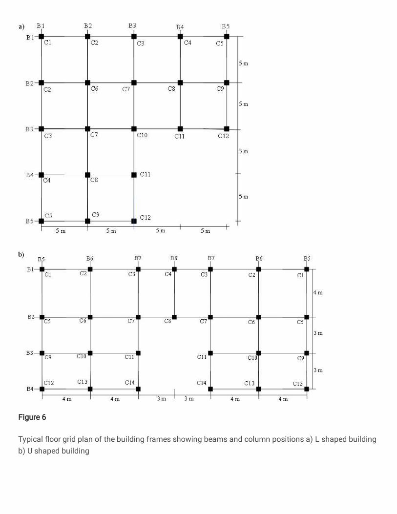
6 Typical floor grid plan of the building frames showing beams and column 1113

positions a) L shaped building b) U shaped 1114

building………………………..……………………………………………….....59 1115

7 Wind profile used wind load analysis a) Velocity profile b) Pressure profile….60 1116

8 Schematic diagram of continuous beam showing the details of curtailments in 1117

bars……………………………………………………………………………….61 1118

9 Design optimization results for L-shaped building frame. (a)convergence curve of 1119

total cost for different grade concrete along with Fe 415 steel.(b)convergence 1120

curve for cost of different parameters for M20 concrete and Fe 415 steel. (c) 1121

Variation of total cost for different concrete and steel grades …………………..62 1122

10 Design optimization results for U-shaped building frame. (a)convergence curve of 1123

total cost for different grade concrete along with Fe 415 steel.(b)convergence 1124

curve for cost of different parameters for M25 concrete and Fe 415 steel. (c) 1125

Variation of total cost for different concrete and steel grades …………………..63 1126

11 Probability distribution for 5000 simulated solutions (L shaped 1127

frame)....………………………………………………………………………….64 1128

12 Probability distribution for 5000 simulated solutions (U shaped 1129

frame)……………………………………………………………………….……65 1130

1131

54

1132

Fig.1. Typical velocity profile of wind moving through a particular terrain (x1, x2=fetch 1133

length; h1, h2=developed height) 1134

1135

1136

1137

1138

1139

1140

Wind

Direction

Vz

Wind

Direction

X

x1

x2

h1

h2=H (Gradient height)

Boundary layer

Building

Z

55

1141

1142

Fig.2.Design acceleration response spectrum of IS 1893-2016(Part-III)[43] 1143

1144

1145

1146

1147

0

0.5

1

1.5

2

2.5

3

0 2 4 6

Sa/

g

Natural period (T,s)

Hard soil

Medium soil

Soft soil

56

1148

1149

Fig. 3.a) Typical reinforcement detail of column section b) Strain diagram of concrete section 1150

when neutral axis lies inside the section c) Strain diagram of concrete section when neutral 1151

axis lies outside the section d) Stress diagram of concrete section when neutral axis lies 1152

outside the section 1153

1154

xu

Dc

0.0035

0.0035

0.002

CL

yi

Compression

i-th row reinforcement

Tension

εci

εci

3Dc/7

xu

a)

b)

c)

N.A

N.A

X

Y

bc

xu

d)

0.446fckg

N.A

57

1155

Fig.4. Flowchart for cost optimization of whole frame 1156

1157

START

STAAD Pro

Design forces for beams Design forces for columns

Optimization

(Algorithm 1, Appendix I)

Optimization

(Algorithm 2, Appendix I)

Optimized design and cost

for individual beams

Optimized design and cost

for individual columns

Optimized design and cost

for entire frame

58

1158

1159

Fig.5.Formwork profile for member cross section: a) Beam b) Column 1160

1161

b

D

bc

Dc

a) b)

59

1162

Fig. 6. Typical floor grid plan of the building frames showing beams and column positions a) 1163

L shaped building b) U shaped building 1164

1165

B1

B2

B3

B4

B5

B1 B2 B3 B5B4

C1 C2

C2

C3

C3

C4

C5

C4 C5

C6 C7

C7

C8

C8

C9

C9

C10 C11

C11

C12

C12

5 m 5 m 5 m 5 m

5 m

5 m

5 m

5 m

B1

B2

B3

B4

B5 B7B6 B8 B7 B6 B5

4 m 4 m 4 m 4 m3 m 3 m

4 m

3 m

3 m

C1 C1C2 C2C3 C3C4

C5 C5C6 C6C7 C7C8

C9 C9C10 C10C11 C11

C12 C12C13 C13C14 C14

a)

b)

60

1166

1167

1168

1169

Fig. 7.Wind profile used wind load analysis a) Velocity profile b) Pressure profile 1170

1171

1172

1173

0

5

10

15

20

25

30

35

40

45

50

0 20 40 60

Hie

ght

(m)

Design wind speeed (Vz) (m/s)

0

5

10

15

20

25

30

35

40

45

50

0 0.5 1 1.5 2

Hie

gh

t (m

)

Design wind pressure (Pd) (KN/m2)

a) b)

61

1174

1175

1176

Fig. 8. Schematic diagram of continuous beam showing the details of curtailments in bars 1177

1178

L

L/3 L/3 L/3

ᶲhb+ ᶲcb

ᶲhtᶲht+ ᶲtt

ᶲhb+ ᶲtb ᶲhb+ ᶲcb

ᶲht+ ᶲtt

ᶲht = hanger bars at top, ᶲtt = extra bars at support top due to tension, ᶲhb = hanger

bars at bottom, ᶲcb = extra bars at support bottom due to compression, ᶲtb = extra

bars at mid-span bottom due to tension

62

1179

Fig. 9. Design optimization results for L-shaped building frame. (a) convergence curve of 1180

total cost for different grade concrete along with Fe 415 steel.(b) convergence curve for cost 1181

of different parameters for M20 concrete and Fe 415 steel. (c) Variation of total cost for 1182

different concrete and steel grades 1183

1184

a) b)

c)

63

1185

Fig. 10. Design optimization results for U-shaped building frame. (a) convergence curve of 1186

total cost for different grade concrete along with Fe 415 steel. (b) convergence curve for cost 1187

of different parameters for M25 concrete and Fe 415 steel. (c) Variation of total cost for 1188

different concrete and steel grades 1189

1190

a) b)

c)

64

1191

Fig.11. Probability distribution for 5000 simulated solutions (L shaped frame) 1192

1193

65

1194

Fig. 12.Probability distribution for 5000 simulated solutions (U shaped frame) 1195

1196

Figures

Figure 1

Typical velocity pro�le of wind moving through a particular terrain (x1, x2=fetch length; h1, h2=developedheight)

Figure 2

Design acceleration response spectrum of IS 1893-2016(Part-III)[43]

Figure 3

a) Typical reinforcement detail of column section b) Strain diagram of concrete section when neutral axislies inside the section c) Strain diagram of concrete section when neutral axis lies outside the section d)Stress diagram of concrete section when neutral axis lies outside the section

Figure 4

Flowchart for cost optimization of whole frame

Figure 5

Formwork pro�le for member cross section: a) Beam b) Column

Figure 6

Typical �oor grid plan of the building frames showing beams and column positions a) L shaped buildingb) U shaped building

Figure 7

Wind pro�le used wind load analysis a) Velocity pro�le b) Pressure pro�le

Figure 8

Schematic diagram of continuous beam showing the details of curtailments in bars

Figure 9

Design optimization results for L-shaped building frame. (a) convergence curve of total cost for differentgrade concrete along with Fe 415 steel. (b) convergence curve for cost of different parameters for M20concrete and Fe 415 steel. (c) Variation of total cost for different concrete and steel grades

Figure 10

Design optimization results for U-shaped building frame. (a) convergence curve of total cost for differentgrade concrete along with Fe 415 steel. (b) convergence curve for cost of different parameters for M25concrete and Fe 415 steel. (c) Variation of total cost for different concrete and steel grades

Figure 11

Probability distribution for 5000 simulated solutions (L shaped frame)

Figure 12

Probability distribution for 5000 simulated solutions (U shaped frame)

Supplementary Files

This is a list of supplementary �les associated with this preprint. Click to download.

APPENDIX.docx