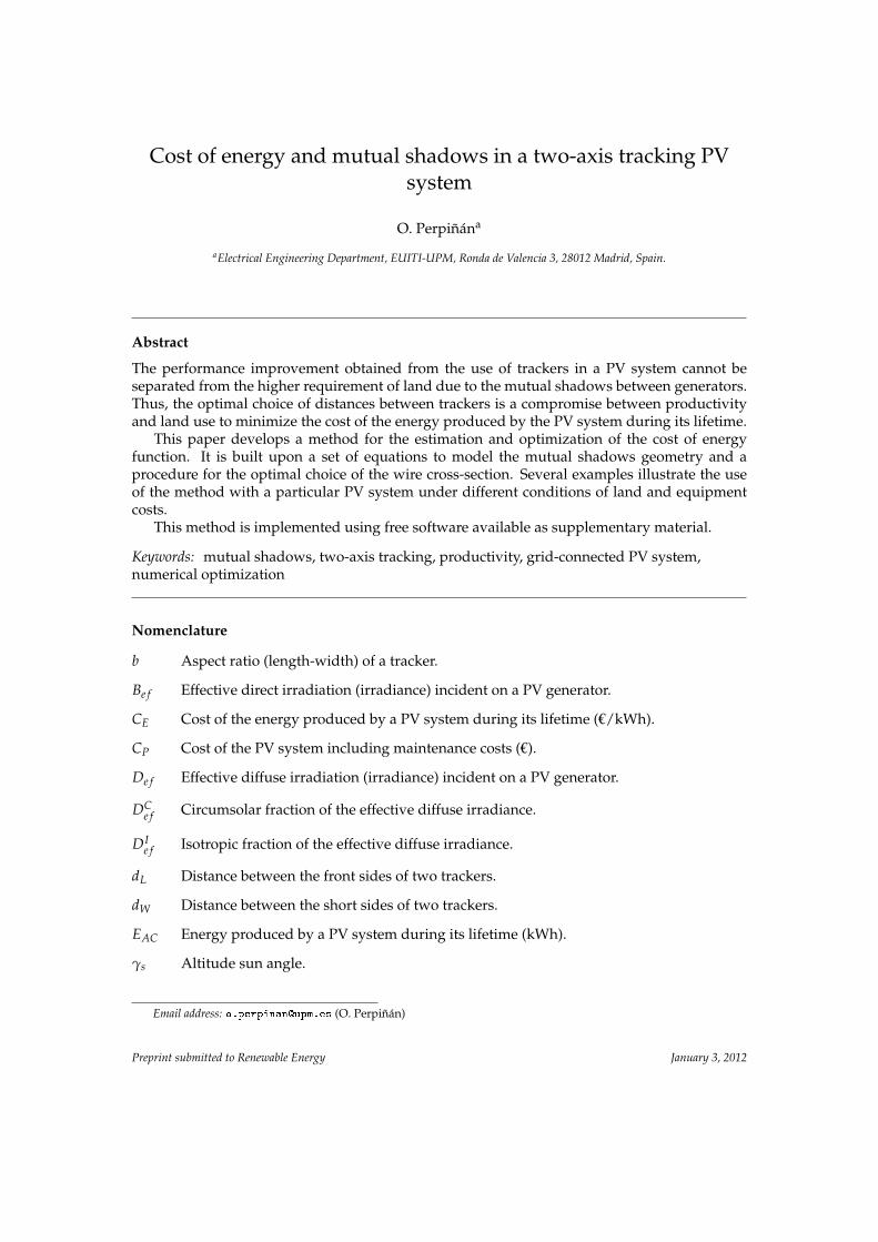
Cost of energy and mutual shadows in a two-axis tracking PV system O. Perpiñán a a Electrical Engineering Department, EUITI-UPM, Ronda de Valencia 3, 28012 Madrid, Spain. Abstract The performance improvement obtained from the use of trackers in a PV system cannot be separated from the higher requirement of land due to the mutual shadows between generators. Thus, the optimal choice of distances between trackers is a compromise between productivity and land use to minimize the cost of the energy produced by the PV system during its lifetime. This paper develops a method for the estimation and optimization of the cost of energy function. It is built upon a set of equations to model the mutual shadows geometry and a procedure for the optimal choice of the wire cross-section. Several examples illustrate the use of the method with a particular PV system under different conditions of land and equipment costs. This method is implemented using free software available as supplementary material. Keywords: mutual shadows, two-axis tracking, productivity, grid-connected PV system, numerical optimization Nomenclature b Aspect ratio (length-width) of a tracker. B ef Effective direct irradiation (irradiance) incident on a PV generator. C E Cost of the energy produced by a PV system during its lifetime (€/kWh). C P Cost of the PV system including maintenance costs (€). D ef Effective diffuse irradiation (irradiance) incident on a PV generator. D C ef Circumsolar fraction of the effective diffuse irradiance. D I ef Isotropic fraction of the effective diffuse irradiance. d L Distance between the front sides of two trackers. d W Distance between the short sides of two trackers. E AC Energy produced by a PV system during its lifetime (kWh). γ s Altitude sun angle. Email address: (O. Perpiñán) Preprint submitted to Renewable Energy January 3, 2012
Transcript
Cost of energy and mutual shadows in a two-axis tracking PVsystem
The performance improvement obtained from the use of trackers in a PV system cannot beseparated from the higher requirement of land due to the mutual shadows between generators.Thus, the optimal choice of distances between trackers is a compromise between productivityand land use to minimize the cost of the energy produced by the PV system during its lifetime.
This paper develops a method for the estimation and optimization of the cost of energyfunction. It is built upon a set of equations to model the mutual shadows geometry and aprocedure for the optimal choice of the wire cross-section. Several examples illustrate the useof the method with a particular PV system under different conditions of land and equipmentcosts.
This method is implemented using free software available as supplementary material.
Preprint submitted to Renewable Energy January 3, 2012
GCR Ground coverage ratio.
Ge f s Effective global irradiation (irradiance) incident on a PV generator including shadows.
GRR Ground requirement ratio.
Ii Current from the i-th tracker.
Iinv Current through the wire from the junction box to the inverter.
koi Coefficients of the efficiency curve of a inverter
L, W Length and width of a tracker.
Lew East-West distance between trackers.
lew East-West distance between trackers (normalized value).
Li Length of the wires from the i-th tracker to the junction box.
Linv Length of the wires from the junction box to the inverter.
Lns North-South distance between trackers.
lns North-South distance between trackers (normalized value).
Pinv Nominal power of the inverter
po Normalized output power of a inverter
ψs Azimuth sun angle.
Re f Albedo irradiance.
ρ Resistivity of the wires.
s Shadows length.
Si Section of the i-th tracker wires.
Sinv Section of the wires from the junction box to the inverter.
θzs Zenith sun angle.
1. Introduction
The concept of a Grid Connected PV System (GCPVS) as an investment product has accel-erated the development of tracking technologies. This quest for increasing the productivity ofGCPVS has a cost: in general, the more precise a tracking method, the less efficient its use ofland due to mutual shadows from nearby trackers.
Thus, the optimal choice of distances between trackers is a compromise between produc-tivity and land use to minimize the cost of the energy produced by the PV system during itslifetime.
The performance of tracking PV systems and mutual shadows models have already beenstudied by several authors. However, nothing has yet been published integrating mutual shad-ows geometry, land and equipment costs, and wiring calculations, to estimate the cost of energy.
2
In this context, this paper develops a method for the estimation and optimization of the costof energy function. It is built upon a set of equations to model the mutual shadows geometryand a procedure for the optimal choice of the wire cross-section.
This document is organized as follows: the section 2 develops a set of equations for thegeometry of shadows and discusses the relation between productivity, shadows and land re-quirement; the section 3 analyzes the wiring design issues in a two-axis tracking systems as aprevious step to the cost of energy calculations; using these concepts the section 4 defines thefunction of the cost of the produced energy and proposes procedures for both the estimationand the minimization of this function. Finally, the section 5 illustrate the estimation and op-timization of the cost function with a PV system under certain conditions of irradiation andtemperature, and with several combinations of land and equipments costs.
Besides, there are three sections at the appendix with a detailed discussion of the wiringcalculations (sections Appendix B and Appendix C) and costs (section Appendix A) issues.
2. Shadows in a two-axis tracking system
The performance of tracking PV systems and mutual shadows models have already beenstudied by other authors: [6] analyze the relation between shadows, area occupation, trackerand plant geometry, limitation of tracking angle and electrical configuration of the generator;[7] include a chapter devoted to geometrical considerations of tracking systems, the energyproduced by each tracking technology and the analysis of mutual shadows; [8] examine thegeometry of shadows in an azimuthal tracking system, applying the results to the design of aPV plant; [9] study the tracking and shading geometry for single vertical axis, single horizontalaxis and two axes, and present simulation results regarding energy production and groundcover; [10] introduce an algorithm that allows the calculation of the optimal location of thePV trackers of a photovoltaic facility on a building of irregular shape, taking into account theshadows caused by the PV trackers and the obstacles that are on the building or surrounding it.
Detailed information about PV tracking, a large set of equations describing the movementof several types of trackers, and a method for mutual shadows calculation can be found in [11].
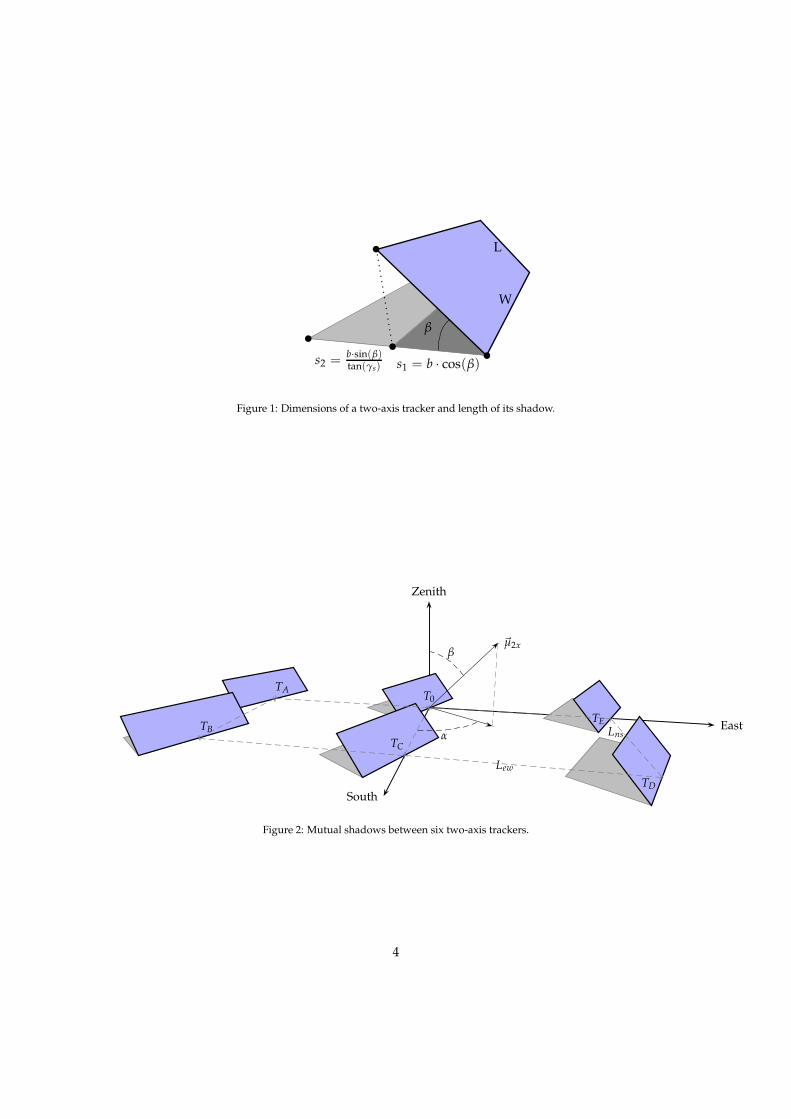
2.1. Geometry of shadowsThe geometry of shadows in a two-axis1 tracking PV system is determined by the next pa-
rameters (figures 1 and 2):
1. The inclination of the PV generator, β, ideally equal to the zenith sun angle, θzs.2. The orientation of the PV generator, α, ideally equal to the solar azimuth, ψs.3. Aspect ratio of the tracker, b : ratio between the length, L, and the width, W, of the tracker.
b =LW
(1)
Henceforth the width W will serve as the normalization factor for the distances between track-ers. Unless otherwise indicated, the distances and lengths of the next sections are normalizedvalues, using lowercase letters to denote this circumstance.
Let’s define a reference coordinate system (X, Y, Z) where the X axis is directed towards theWest, the Y axis towards the South (in the north hemisphere) and the Z axis towards the zenith(figure 2). Let T0 be a tracker at the origin of coordinates, (0, 0, 0) and let TX be a tracker located
1The subsequent analysis is restricted to two-axis tracking systems. The interested reader can find detailed equationsof the geometry of several tracking systems in [11]
3
b
bb
bβ
s1 = b · cos(β)s2 =b·sin(β)tan(γs)
L
W
Figure 1: Dimensions of a two-axis tracker and length of its shadow.
Zenith
South
East
β
α
Lew
Lns
T0
TC
TD
TE
TA
TB
~µ2x
Figure 2: Mutual shadows between six two-axis trackers.
4
T0
d L
dWs
TX
Figure 3: Distances between two trackers
at (x, y, z) (figure 3). The shadows occurrence on T0 due to TX is defined by the simultaneousfulfilling of three conditions:
1. dW < 1, where dW is the distance between the short sides of both trackers.2. s > dL, where s is the shadows length and dL is the distance between the front side of both
trackers.3. The tracker TX is situated between the sun and the tracker T0.
In order to check these conditions it is compulsory to compute the distances, dL and dW , andthe shadows length, s. This length is composed of two segments (figure 1):
s = s1 + s2 (2)s1 = b · cos(β) (3)
s2 =b · sin(β) + z
tan(γs)(4)
where z is the relative height of the tracker TX , and γs is the altitude sun angle. With idealsun-tracking β + γs = π/2, and therefore:
s =b
cos β+ z · tan β (5)
The distances dL and dW can be easily calculated with the cross product of two vectors asdistances between parallel lines. Let r1 be a line with a director vector ~ur1 and A a point inthis line, and r2 a line whose vector ~ur2 is parallel to ~ur1 , and B a point located in r2. Then, thedistance between r1 and r2 is:
d(r1, r2) =| ~AB× ~ur1 ||~ur1 |
(6)
The distance dW is calculated as the distance between the lines passing through the centersof the trackers pointing at the sun. Thus, A = (0, 0, 0), B = (x, y, 0) and ~ur1 = (sin ψs, cos ψs, 0).
dW = |x cos ψs − y sin ψs| (7)
5
The distance dL is the distance between the lines passing through the centers of the trackersbut whose direction is normal to the sun vector, ~ur1 = (cos ψs,− sin ψs, 0)
dL = |x sin ψs + y cos ψs| (8)
The third condition can be checked with the sign of the scalar product ~AB · ~ur = x sin ψs +y cos ψs. Thus, this condition can be stated as:
x sin ψs + y cos ψs > 0 (9)
In order to save computation time, it should be noted that the left term of this equation isthe right term of the equation (8) before taking absolute values.
When the three conditions apply (dW < 1, dL < s and equation (9)), the tracker at the originis being shaded by the tracker TX with a shadow factor, SF:
SF =(1− dW) · (s− dL)
b· sin(γs)
sin(γs + β)(10)
This shadow factor SF is calculated as the ratio between the shaded area and the total area ofthe generator. Therefore SF is zero when no shadow is received. The first fraction of this productaccounts for the shadow ratio on the horizontal plane, while the second fraction projects it uponthe generator plane.
The shadow factor with ideal tracking (β + γs = π/2, equation (5)) and coplanar trackers(z = 0) is:
SF =(1− dW) · (s− dL)
s(11)
2.2. Shadows and productivityThe power reduction for a given shade fraction depends on the electrical configuration of
the PV system. This relation is comprised between two extremes [12]. The upper or pessimisticbound assumes that shading of any part of the PV generator produces zero output power. Thelower or optimistic bound assumes that power losses due to shadows are proportional to theshaded beam radiation. Several references [13, 14, 16, 17, 18] show the complexity and limits as-sociated with the electrical models of shaded generators. Thus, the generalization of the varietyof cases comprised between these two bounds is not easily feasible (although some experimen-tal models have been already proposed [19]).
Gordon and Wenger [12] show that in a yearly basis the optimistic case is closer to a “basecase” where the power of a PV module is zero when it is shaded, as an approximation to the useof bypass diodes. This approach is particularly reasonable for large generators where the effectin the global I-V characteristic of the modification of the I-V curve in some modules is lowerthan in small generators.
Hence, in this work a modified optimistic formulation is applied: the shadow factor propor-tionally reduces both the beam and the circumsolar diffuse irradiance components:
Ge f s = DIe f + Re f + (DC
e f + Be f ) · (1− SF) (12)
where Ge f s is the global effective irradiance including shadows, DIe f and DC
e f are, respectively,the isotropic and circumsolar fractions of the effective diffuse irradiance, Be f is the direct irra-diance and Re f is the albedo irradiance.
This procedure has been sucessfully validated using performance data of a 6.02 MWp two-axis tracking GCPVS located in Spain [20]. However, this model imposes uncertainty in thesubsequent calculation steps. Therefore, the estimation and optimization results (section 5.2and 5.3) must be interpreted in this context.
6
2.3. The ground requirement ratioOne of the tasks of the design of a PV tracking system is to place the set of trackers. This
task must cope with the compromise of minimizing the losses due to mutual shadows whilerequiring the minimum land area.
A suitable approach to this problem is to simulate the planned system for a set of distancesbetween the trackers of the plant. Without any additional constraint, the optimum design maybe the one which achieves the highest productivity with the lowest ground requirement ratio.This definition of the optimization problem is not complete since the land requirements andthe costs of wiring and equipments should be included as additional constraints. They areconsidered in section 4.
The area of the PV generator and the total land requirement are commonly related withthe Ground Coverage Ratio (GCR) [9, 8, 12]. This ratio quantifies the percentage of land beingeffectively occupied by the system. In order to focus on the land area required, the inverse ofthis ratio, the Ground Requirement Ratio (GRR), is preferable. The GRR is the ratio between theground area required for installing the whole set of trackers and the generator area.
For this model GRR = lns ·lewb . Both lew and lns are normalized distances, related to the
absolute distances through lew = LewW and lns =
LnsW . Therefore, GRR = Lew ·Lns
L·W .A simplified two-axis tracking PV plant can be modeled with a group of six coplanar track-
ers, distributed in a matrix of two rows in the North-South direction and three columns in theEast-West direction (figure 2). Each tracker is named according to its position in the group. Forexample, a TA tracker could be shaded by a tracker on the East direction (T0) and another onein the South direction (TB). The model calculates the shaded irradiance for each of the six typesof trackers. The average irradiance incident on a PV tracking system is the weighted averageof the irradiance of the six trackers of the group. The weights are the proportion of trackers ineach position.
An example will clarify this approach. In the PV plant defined in the figure A.8, there are 10trackers T0 (for example, the tracker no.2 of the junction box no.1)2, 2 trackers TC (tracker no. 4of the junction box 1 and tracker no. 3 of the junction box no.2), 5 trackers TA (for example, thetracker no.2 of the junction box 4), etc. Thus, the model will calculate six different irradiances:Ge f ,0 for the trackers T0, Ge f ,A for the trackers TA and so on. The average irradiance of the groupof 24 trackers of the figure A.8 is:
Ge f ,av = 1/24 ·(
10 · Ge f ,0 + 5 · Ge f ,A + Ge f ,B + 2 · Ge f ,C + Ge f ,D + 5 · Ge f ,E
)(13)
3. Wiring design in a tracking PV system
A grid connected PV system is electrically divided in two parts: DC (from the PV modules tothe input of the inverter) and AC (from the output of the inverter to the grid connection point).The distances between a PV generator and its associated inverter, and between the inverter andthe electrical grid are design parameters to be defined as a compromise between energy lossesand wiring costs.
It is possible to show that (section Appendix B), upon a certain voltage threshold (around475 V for three-phase systems), a DC distribution scheme (the inverters are situated next to thegrid connection point) is better than a AC distribution scheme (the inverters are situated next tothe PV generators, and the AC wiring conducts the electricity to the grid.) Due to the large sizes
2In a large PV plant there will be a high number of trackers in the T0 location.
7
of the tracking PV plants, the input voltage of the inverters is commonly over this threshold.Thus, the optimization procedure to be described will assume that a DC distribution scheme isadopted.
The wiring design involves the selection of a wire section adequate to the electrical current(heat dissipation) and distance (voltage losses). Let’s assume that the cost of the wire is propor-tional to the conductor volume, and that the voltage drop to the inverter is the same from everytracker. Under such conditions, it is possible to show (section Appendix C) that the optimumsections to obtain a certain global voltage drop ∆U are calculated with (figures A.8 and C.10):
∆Uinv =∆U
1 +√
∑ni=1 L2
i ·IiL2
inv ·Iinv
(14)
∆Uinv = 2 · ρ · Linv · IinvSinv
(15)
∆Ui = 2 · ρ · Li · IiSi
(16)
where Iinv is the current through the inverter wire, Ii is the current from the i-th tracker (Iinv =∑n
i=1 Ii.), Linv is the length of the wires from the junction box to the inverter, Li is the length ofthe wires from the i-th tracker to the junction box, Sinv is the section of the inverter wires, Si isthe section of the i-th tracker wires and ρ is the electrical resistivity of the wires.
With these equations the wire section of each part of the system can be calculated to obtaina certain value of ∆U. These results have to be checked and conveniently corrected under twocriteria:
• Only a set of normalized sections is available. Thus Si ∈ (4, 6, 10, 16, 25, 35, 50, 70, 95, ...)mm2.
• Each type of conductor is characterized by a maximum admissible current dependent onthe kind of installation. These values are commonly documented in national regulations(for example, [21] for Spain).
4. The cost of energy
4.1. DefinitionThe cost of the energy produced by a PV plant during its lifetime, CE, (€/kWh), is the ratio
between the cost of the PV system including maintenance costs, CP (€), and the energy producedby a PV system during its lifetime, EAC (kWh):
CE =CP
EAC(17)
CP can be calculated with Cp = Cc + CA + CPV , where:
• Cc is the cost dependence on the wiring length (cable costs) modeled by a linear functionCc = kc · Lc, where the constant kc is the cost of cable per unit length (figure A.9) and Lc isthe length of cable.
• CA is the cost dependence on the required area (land costs), modeled with CA = kA · At,where the constant kA is the cost of land per unit area, and At is the total area (calculatedwith the distances between trackers, Lew and Lns).
8
• CPV is a constant term related with the cost of the PV generator, inverter, trackers andthose elements whose size and quantity are not influenced by the distances between track-ers (equipment costs).
Eac is the aggregated result of the procedure outlined in the table 1. Since one of the stepsof this procedure depends on the distances between trackers, both EAC and CP are functions ofthe distances LEW and LNS.
4.2. Calculation procedureSince this investigation is focused on the distances between trackers, the calculation pro-
cedure of the cost of energy assumes that the configuration of the PV plant has been alreadydefined: the PV generator and inverter power; the number and type of modules, inverters andtrackers; the number of modules in series and parallel; etc. With this information, the procedureis:
1. For a pair of LEW and LNS distances, the energy produced by a group of trackers withmutual shadows is calculated following the table 1.
2. The wiring section of each circuit of the system is calculated. Both the voltage drop andthe set of normalized sections constraints are applied (section 3).
3. The required land area is calculated with the distances between generators and the num-ber of trackers included in the system (section 2.3).
4. The cost of the plant is computed as the sum of costs of wire, land and equipments (section4.1).
5. Finally, the result is the ratio between the cost of the plant and the produced energy alongits lifetime.
4.3. Numerical optimization of the CE functionAlthough displaying the function CE over a grid of distances is useful to understand its
behavior (figure 4), the optimum configuration is more efficiently found with an optimizationalgorithm. The optimization of the distances between trackers means solving the problem inwhich the objective function (CE) is minimized by systematically choosing the values of realvariables from within an allowed set.
The optimization problem is limited to a feasible region defined by several constraints:
• The separation distances must be greater than the dimensions of the trackers: LEW > Wand LNS > L.
• The voltage drop across a circuit must equal a predefined value (1.5% for example).
• Only a set of wiring sections are allowed (section 3).
The iteration begins with a starting pair of distances (Lew, Lns) in the feasible region. For thisinitial pair the cost of energy is calculated following the procedure outlined at section 4.2. Withan optimization algorithm, a new pair of distances is selected and the calculation procedure isrepeated until a convergence criterion is achieved.
For any given optimization problem, it is sensible to compare several of the available algo-rithms that are applicable to that problem. The performance of each algorithm strongly dependsupon the problem to be solved. Moreover, not only the precision and robustness are importantbut also the computation speed and cost must be considered when evaluating a candidate.
9
Step Method
Sun and trackers geometry Set of equations as provided in [2]
Decomposition of monthly means ofdaily global horizontal irradiation
Correlation between diffuse fractionof horizontal radiation and clearnessindex [22]
Estimation of irradiance Ratio of global irradiance to dailyglobal irradiation [23]
Estimation of irradiance on inclinedsurface
The direct irradiance is calculated withgeometrical equations. The estimationof the diffuse component makes use ofthe anisotropic model [24]
Albedo irradiance Isotropic diffuse irradiance withreflection factor equal to 0.2.
Effects of dirt and angle of incidenceEquations proposed in [25]. A lowconstant dirtiness degree has beensupposed (2%)
Shading effects
Only the circumsolar diffuse anddirect irradiance components areproportionally reduced with theshadow factor, SF (equation ((12)))
PV generator
Identical modules withdVoc/dTc = 0, 475 %
°C andNOCT = 47°C. The MPP point iscalculated with the method by Ruiz(as published in [15]).
Efficiency of the inverter
Equation proposed in [26]:
ηinv =po
po + ko0 + ko
1 po + ko2 p2
o(18)
where po = Pac/Pinv is the normalizedoutput power of the inverter. Thecharacteristic coefficients of theinverters for the example are:ko
0 = 0.01, ko1 = 0.025, ko
2 = 0.05.
Other losses
• Average tolerance of the set ofmodules, 3%.
• Module parameter disperssionlosses, 2%.
• Joule losses due to the wiring,1.5%.
• Average error of the MPPalgorithm of the inverter, 1%.
• Losses due to the MVtransformer, 1%.
• Losses due to stops of thesystem, 0.5%.
Table 1: Calculation procedure for the estimation of energy produced by a PV system from daily global horizontalirradiation data
10
Although a systematic comparison of optimization algorithms is beyond the scope of thispaper, two different methods have been tested: the Nelder-Mead and the COBYLA algorithms,both as implemented in the NLopt package [27].
The Nelder-Mead (or downhill simplex) method [28] is a robust and quite simple techniquewhich approximates a local optimum of a problem with N variables when the objective functionvaries smoothly and is unimodal.
The COBYLA method (Constrained Optimization BY Linear Approximations) [29] for deriva-tive free optimization with nonlinear inequality and equality constraints constructs successivelinear approximations of the objective function and constraints via a simplex of n+1 points (inn dimensions), and optimizes these approximations in a trust region at each step.
5. Numerical results
The next sections illustrate the estimation (section 5.2) and optimization (section 5.3) of theCE function with a PV system under certain conditions of irradiation and temperature, and withseveral combinations of land and equipments costs. This information is related in the sectionAppendix A.
The use of a particular configuration for the PV system and meteorological conditions mayrepresent a loss of generality. However, since the aim of this paper is to propose a method (andassociated software) to estimate and optimize the CE function, the examples provide a betterway to understand the development.
5.1. SoftwareThe methods described in this paper have been implemented using the free software envi-
ronment R [1] and several contributed packages, namely the solaR package [2] for the solar ge-ometry, irradiation and PV energy calculations, the nloptr package for the optimization tasks,and the lattice [3], latticeExtra [4] and colorspace [5] packages as visualization tools.
The code is available at http://procomun.wordpress.com/documentos/articulos and asa supplementary material to this paper.
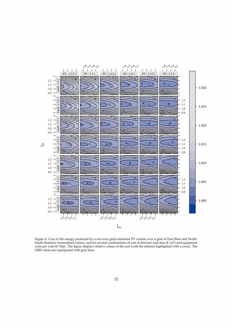
5.2. Output of the CE functionThe figure 4 shows the output of the CE function for the system described in the section
Appendix A over a grid of East-West and North-South distances, and for several combinationsof land and PV equipment costs. The figure displays relative values of the cost (with the minimahighlighted with a cross). The GRR values are superposed with gray lines.
The minima is located inside an ellipse with its major axis along the lEW axis. Thus, thevalues of the function are less sensitive to changes in the East-West distances than in the North-South distances. The figure 5 shows that the minima is easily located following the curves oflNS (right panel) although several values of lEW give results very close to the minima. Therefore,the designer can choose the LEW distance more flexibly than the LNS to achieve the optimal costof energy value.
The location of the minima moves for each combination of land and equipments costs. Forthe meteorological conditions of this example, it can be found near lNS ' 1.1 for all the panels,but goes over the whole range of lEW , from 1.7 for low values of equipment costs and highvalues of land costs, to 2.2 for the opposite combination. Besides, the minima traverse the GRRlines from GRR ' 4 for high land costs and low values of equipments costs, to GRR ' 6 for theopposite combination.
Figure 4: Cost of the energy produced by a two-axis grid-connected PV system over a grid of East-West and North-South distances (normalized values), and for several combinations of cost of land per unit area (€/m2) and equipmentcosts per watt (€/Wp). The figure displays relative values of the cost (with the minima highlighted with a cross). TheGRR values are superposed with gray lines.
Figure 5: Subset of the figure 4 (land costs of 2 €/m2) and equipments costs of 3,5 €/W. The left panel shows thebehavior with the North-South distance and the right panel displays the relation with the East-West distance. Eachcolor corresponds to a GRR range.
These results must be interpreted in the context of the uncertainty limitations due to theenergy estimation methods (table 1 and section 2.2). In this context, small departures from theoptimum are indistinguishable.
This observation, which adds more flexibility to the design tasks, is also important whencomparing the results from different optimization algorithms.
5.3. Numerical optimization of the CE functionIf the equipment cost is 2,5 €/W and the land cost is 1,5 €/m2 the Nelder-Mead algorithm
converges after 70 iterations with lEW = 2.114 (LEW = 48,853 m), lns = 1.196 (LNS = 27,63 m)and CE = 7,717 c€/kWh. The COBYLA algorithm converges after 35 iterations with approxi-mately the same results.
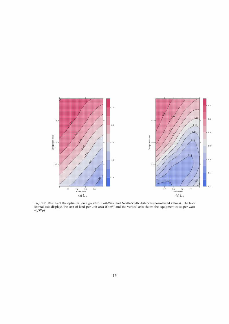
The figures 6 (GRR values) and 7 (lEW and lNS, normalized distances) display the results ofthe COBYLA algorithm for several combinations of land and equipment costs.
The GRR values range from GRR ' 6.5 for low values of land costs and high equipmentcosts to GRR ' 5 for the opposite combination, with intermediate values for the rest of thegrid. These results agree with the analysis of the figure 4.
The lEW values (figure 7a) range from lEW ' 1.8 to lEW ' 2.2. The lNS distance (figure 7b)varies along a smaller interval: from lNS ' 1.12 to lEW ' 1.24. Once again this behavior wasanticipated with the figures 4 and 5.
13
Land costs
Equ
ipm
ent c
osts
3.5
4.0
4.5
2.2 2.4 2.6 2.8
5.1
5.2
5.3
5.4
5.5
5.6
5.7
5.8
5.9
6.0
6.1
6.2
6.3
6.4
6.4
5.0
5.2
5.4
5.6
5.8
6.0
6.2
6.4
6.6
Figure 6: Results of the optimization algorithm: Ground Requirement Ratio. The horizontal axis displays the cost ofland per unit area (€/m2) and the vertical axis shows the equipment costs per watt (€/Wp)
6. Conclusions
The performance improvement obtained from the use of trackers in a PV system cannot beseparated from the higher requirement of land due to the mutual shadows between generators.Thus, the optimal choice of distances between trackers is a compromise between productivityand land use to minimize the cost of the energy produced by the PV system during its lifetime.
This paper develops a method for the estimation and optimization of the cost of energyfunction. It is built upon a set of equations to model the mutual shadows geometry and aprocedure for the optimal choice of the wire cross-section. Several examples illustrate the useof the method with a particular PV system under different conditions of land and equipmentcosts.
For this particular example, the minima is located inside an ellipse with its major axis alongthe lEW axis. In other words, the values of the function are less sensitive to changes in the East-West distances than in the North-South distances. Therefore, the designer can choose the LEWdistance more flexibly than the LNS to achieve the optimal cost of energy value.
The location of the minima moves for each combination of land and equipments costs. TheGRR values range from GRR ' 6.5 for low values of land costs and high equipment costs toGRR ' 5 for the opposite combination, with intermediate values for the rest of the grid. ThelEW values range from lEW ' 1.8 to lEW ' 2.2. The lNS distance varies along a smaller interval:from lNS ' 1.12 to lEW ' 1.24.
These results must be interpreted in the context of the uncertainty limitations due to theenergy estimation methods. In this context, small departures from the optimum are indistin-guishable.
This method and the examples are implemented using free software. The code is available
14
Land costs
Equ
ipm
ent c
osts
3.5
4.0
4.5
2.2 2.4 2.6 2.8
1.85
1.90
1.95
2.00
2.05
2.10
2.15
2.20
2.20
1.8
1.9
2.0
2.1
2.2
(a) Lew
Land costs
Equ
ipm
ent c
osts
3.5
4.0
4.5
2.2 2.4 2.6 2.8
1.14
1.15
1.16
1.17
1.17
1.18
1.18
1.19
1.20
1.21
1.221.23
1.12
1.14
1.16
1.18
1.20
1.22
1.24
(b) Lns
Figure 7: Results of the optimization algorithm: East-West and North-South distances (normalized values). The hor-izontal axis displays the cost of land per unit area (€/m2) and the vertical axis shows the equipment costs per watt(€/Wp)
15
as supplementary material.
Bibliography
[1] R Development Core Team, . R: A Language and Environment for Statistical Computing.R Foundation for Statistical Computing; Vienna, Austria; 2011. ISBN 3-900051-07-0; URLhttp://www.R-project.org.
[2] Perpinan, O.. solaR: Calculation of Solar Radiation and PV Systems.; 2011. R packageversion 0.24; URL http://cran.r-project.org/web/packages/solaR/.
[3] Sarkar, D.. Lattice: Multivariate Data Visualization with R. New York: Springer; 2008.ISBN 978-0-387-75968-5; URL http://lmdvr.r-forge.r-project.org.
[4] Sarkar, D., Andrews, F.. latticeExtra: Extra Graphical Utilities Based on Lattice; 2011. URLhttp://R-Forge.R-project.org/projects/latticeextra/.
[5] Ihaka, R., Murrell, P., Hornik, K., Zeileis, A.. colorspace: Color Space Manipulation;2011. R package version 1.1-0; URL http://CRAN.R-project.org/package=colorspace.
[6] Gordon, J.M., Kreider, J.F., Reeves, P.S.. Tracking and stationary flat plate solar collec-tors: Yearly collectible energy correlations for photovoltaics applications. Solar Energy1991;47(4).
[7] Macagnan, M.H.. Caracterización de la radiación solar para aplicaciones fotovoltaicas enel caso de madrid. Ph.D. thesis; Instituto de Energía Solar, UPM; 1993.
[8] Lorenzo, E., Pérez, M., Ezpeleta, A., Acedo, J.. Design of tracking photovoltaic sys-tems with a single vertical axis. Progress in Photovoltaics: Research and Applications2002;10(8):533–543. doi:\bibinfo{doi}{10.1002/pip.442}.
[9] Narvarte, L., Lorenzo, E.. Tracking and ground cover ratio. Progress in Photovoltaics:Research and Applications 2008;16(8):703–714. doi:\bibinfo{doi}{10.1002/pip.847}.
[10] Díaz-Dorado, E., Suárez-García, A., Carrillo, C.J., Cidrás, J.. Optimal distribution forphotovoltaic solar trackers to minimize power losses caused by shadows. Renewable En-ergy 2011;36(6):1826 – 1835. doi:\bibinfo{doi}{DOI:10.1016/j.renene.2010.12.002}.
[11] Perpiñán, O.. Energía Solar Fotovoltaica. 2011. URL http://procomun.wordpress.com/
documentos/libroesf/.
[12] Gordon, J.M., Wenger, H.J.. Central-station solar photovoltaic systems: field layout,tracker, and array geometry sensitivity studies. Solar Energy 1991;46(4):211–217.
[13] Woyte, A., Nijs, J., Belmans, R.. Partial shadowing of photovoltaic arrays with differentsystem configurations: literature review and field test results. Solar Energy 2003;74:217–233. doi:\bibinfo{doi}{10.1016/S0038-092X(03)00155-5}.
[14] Quaschning, V., Hanitsch, R.. Numerical simulation of current-voltage characteristics ofphotovoltaic systems with shaded solar cells. Solar Energy 1996;56(6).
[15] Alonso-García, M. C.. Caracterización y modelado de asociaciones de dispositivos foto-voltaicos. Ph.D. thesis; CIEMAT; 2005
[16] Alonso-García, M.C., Herrmann, W., Böhmer, W., Proisy, B.. Thermal and electricaleffects caused by outdoor hot-spot testing in associations of photovoltaic cells. Progress inphotovoltaics: research and applications 2003;11:293–307. doi:\bibinfo{doi}{10.1002/pip.490}.
[17] Alonso-García, M.C., Ruíz, J.M., Chenlo, F.. Experimental study of mismatch and shadingeffects in the I-V characteristics of a photovoltaic module. Solar Energy 2006;90(3):329–340.
[18] Alonso-García, M.C., Ruíz, J.M., Herrmann, W.. Computer simulation of shading effectsin photovoltaic arrays. Renewable Energy 2006;31(12):1986–1993. doi:\bibinfo{doi}{10.1016/j.renene.2005.09.030}.
[19] Martínez-Moreno, F., Muñoz, J., Lorenzo, E.. Experimental model to estimate shadinglosses on PV arrays. Solar Energy Materials and Solar Cells 2010;94(12):2298 – 2303. doi:\bibinfo{doi}{DOI:10.1016/j.solmat.2010.07.029}.
[20] Perpiñán, O.. Statistical analysis of the performance and simulation of a two-axis trackingPV system. Solar Energy 2009;83(11):2074–2085. doi:\bibinfo{doi}{10.1016/j.solener.2009.08.008}. URL http://oa.upm.es/1843/1/PERPINAN_ART2009_01.pdf.
[21] Ministerio de Ciencia y Tecnología, . Real Decreto 842/2002, de 2 de agosto, por el quese aprueba el Reglamento electrotécnico para baja tensión. 2002. URL http://www.ffii.
[22] Page, J.K.. The calculation of monthly mean solar radiation for horizontal and inclinedsurfaces from sunshine records for latitudes 40n-40s. In: U.N. Conference on New Sourcesof Energy; vol. 4. 1961, p. 378–390.
[23] Collares-Pereira, M., Rabl, A.. The average distribution of solar radiation: correlationsbetween diffuse and hemispherical and between daily and hourly insolation values. SolarEnergy 1979;22:155–164.
[24] Hay, J.E., McKay, D.C.. Estimating solar irradiance on inclined surfaces: A review andassessment of methodologies. Int J Solar Energy 1985;(3):203–.
[25] Martin, N., Ruíz, J.M.. Calculation of the PV modules angular losses under field condi-tions by means of an analytical model. Solar Energy Materials & Solar Cells 2001;70:25–38.
[26] Jantsch, M., Schmidt, H., Schmid, J.. Results on the concerted action on power con-ditioning and control. In: 11th European photovoltaic Solar Energy Conference. 1992, p.1589–1592.
[27] Johnson, S.G.. The NLopt nonlinear-optimization package; 2011. URL http://
ab-initio.mit.edu/nlopt.
[28] Nelder, J.A., Mead, R.. A simplex method for function minimization. Computer Journal1965;7:308–313.
[29] Powell, M.J.D.. Direct search algorithms for optimization calculations. ActaNumerica 1998;7:287–336. doi:\bibinfo{doi}{10.1017/S0962492900002841}. http://
Figure A.8: Layout of the PV system. For illustrative purposes, the wires are labeled with the values of lengths andcross-sections corresponding to LEW = 50 m and LNS = 30 m.
[30] Perpiñán, O., Lorenzo, E., Castro, M.A., Eyras, R.. Energy payback time of grid connectedPV systems: comparison between tracking and fixed systems. Progress in Photovoltaics:Research and Applications 2009;17:137–147. doi:\bibinfo{doi}{10.1002/pip.871}.
Appendix A. Data for the examples
This section provides information of the PV system, land and equipment costs, irradiationand temperature conditions, used in part of the paper to illustrate the definition of the CE func-tion in the section 5.
The PV system is composed of 24 two-axis trackers. Each of the trackers (L = 9,8 m, W =23,11 m) supports a PV array of 132 modules of 200 Wp with 12 modules in series and 11 inparallel. Detailed information about this system can be found in a previous paper [30].
A group of four trackers forms a PV generator with a nominal power of 105,6 kWp. Eachgroup feeds one of a set of six inverters of 100 kWp. The inverters are hosted in a buildingapproximately at the geometrical center of the plant (figure A.8)
This system is simulated with the meteorological conditions of a site located at Sevilla (lati-tude φ = 37.2°) (table Appendix A)
18
Parameter Jan Feb Mar Apr May Jun Jul Aug Sep Oct Nov Dec
Table A.2: Meteorological data (monthly means of global irradiation and ambient temperature) of Sevilla, Spain.
Section (mm²)
Uni
tary
Cos
t (eu
ro/m
)
20
30
40
50
60
70
0 20 40 60 80
● ●
●
●
●
●
●
●
●
RZConduitRZBuried
●
Figure A.9: Unitary costs for different sections of free-halogen cable (from the PREOC database).
The information for the cable costs have been extracted from the PREOC database. Thisdatabase is available online 3 and it is a frequently used reference for industrial and civil worksprices in Spain. The figure A.9 displays the unitary costs for a free-halogen cable either buriedor with conduits.
The equipment cost range (from 2,5 €/W to 5 €/W) is inspired from the SolarBuzz web-page4 while the land cost range (from 1,5 €/m2 to 4 €/m2)5 is derived from several professionalforums6.
Appendix B. AC versus DC
Let’s show that, upon a certain voltage threshold, a DC distribution scheme (the inverters aresituated next to the grid connection point) is better than a AC distribution scheme (the inverters
3http://www.preoc.es/4http://solarbuzz.com/facts-and-figures/retail-price-environment5For example, 2,5 €/m2 is the result of a yearly land rental of 1000€ per hectare during 25 years.6For example http://www.solarweb.net.
are situated next to the PV generators, and the AC wiring conducts the electricity to the grid.)Some assumptions are needed for a clearer proof:
1. The connection to the distribution grid is three-phase through three-phase inverters with-out neutral wire.
2. The efficiency of the inverter is almost constant with a value of 0.95.3. The reactive power of the inverter is negligible.4. The admissible voltage drop is ∆V = 1.5% · Vnom, where Vnom is the nominal voltage for
each part. For the AC part is Vnom = 400 V.5. Both distribution schemes use a wire with the same conductivity, σ.
The intersection point is found when both distribution schemes require the same mass ofwire:
2 · Sdc · Lw = 3 · S3ac · Lw (B.1)
where Lw is the wire length, Sdc is the section for the DC distribution scheme and Sac is thesection for the AC distribution scheme.
The DC section is calculated with:
Sdc =2 · Lw · Idcσ · ∆Vdc
(B.2)
and the AC section is calculated with:
S3ac =
√3 · Lw · I3ac
σ · ∆V3ac(B.3)
where the assumptions no.3 and no.5 have been considered.These equations can be rewritten with the relations between electrical power, voltage and
current (assumption no.4):
Sdc =2 · Lw · Pdc
σ · 1.5% ·V2dc
(B.4)
S3ac =Lw · Pac
σ · 1.5% ·V2ac
(B.5)
Equation (B.1) is now:
2 · 2 · Lw · Pdc
σ · 1.5% ·V2dc
= 3 · Lw · Pac
σ · 1.5% ·V2ac
(B.6)
It can be simplified using the assumption no.2:
4V2
dc=
3 · ηinvV2
ac(B.7)
which leads to the final result (with Vac = 400 V and ηinv = 0.95):
Vdc ' 473 V (B.8)
Thus, if the average Vmpp voltage of the PV generator is above 473 V, the DC distributionscheme is preferable to the AC distribution scheme to optimize the total mass of wire.
20
Junction
Box
Inverter
Linv, Iinv
Tracker 1
L1, I1
Tracker 2
L2, I2
Figure C.10: Wire lengths and currents in a PV system with two trackers feeding a common inverter through a junctionbox.
Appendix C. Wire section optimization
In order to calculate the wire section for each part of the system, two assumptions areneeded:
• The cost of the wire is proportional to the conductor volume.
• The voltage drop to the inverter is the same from every tracker.
For two generators feeding a common inverter (figure C.10), the voltage drops are:
∆Uinv + ∆U1 = ∆U (C.1)∆Uinv + ∆U2 = ∆U (C.2)
where ∆Uinv stands for the voltage drop from the junction box to the inverter, ∆Ui stands for thevoltage drop from the tracker i to the junction box, and ∆U is the voltage drop from a tracker tothe inverter. These voltage drops can be calculated with:
∆Uinv = 2 · ρ · Linv · IinvSinv
(C.3)
∆Ui = 2 · ρ · Li · IiSi
(C.4)
where Iinv is the current through the inverter wire, Ii is the current from the i-th tracker, Linv isthe length of the wires from the junction box to the inverter, Li is the length of the wires fromthe i-th tracker to the junction box, Sinv is the section of the wires from the junction box to theinverter, Si is the section of the i-th tracker wires and ρ is the electrical resistivity of the wires.
Of course, Iinv = I1 + I2. The total wire volume, assuming a DC distribution schema (sectionAppendix B), is:
With the equations (C.1) and (C.2) the wire volume is:
Vol = 4 · ρ ·(
L2inv · Iinv
∆Uinv+
L21 · I1
∆U − ∆Uinv+
L22 · I2
∆U − ∆Uinv
)(C.7)
21
The optimum choice of sections is the result of dVoldU = 0.
L2inv · Iinv
∆Uinv=
L21 · I1 + L2
2 · I2
∆U − ∆Uinv(C.8)
and, therefore,∆U − ∆Uinv
∆Uinv=
L21 · I1 + L2
2 · I2
L2inv · Iinv
(C.9)
which can be rewritten to:∆Uinv =
∆U
1 +√
L21·I1+L2
2·I2
L2inv ·Iinv
(C.10)
This last equation can be generalized for a higher number of trackers:
∆Uinv =∆U
1 +√
∑ni=1 L2
i ·IiL2
inv ·Iinv
(C.11)
where Iinv = ∑ni=1 Ii.
With the equation (C.1) to (C.4) and (C.11), the wire section of each part of the system can becalculated to obtain a certain value of ∆U. These results have to be checked and convenientlycorrected under two criteria:
• Only a set of normalized sections is available. Thus Si ∈ (4, 6, 10, 16, 25, 35, 50, 70, 95, ...)mm2.
• Each type of conductor is characterized by a maximum admissible current dependent onthe kind of installation. These values are commonly documented in national regulations(for example, [21] for Spain).