Ecological Modelling, 27 (1985) 45-68 45 Elsevier Science Publishers B.V., Amsterdam - Printed in The Netherlands
ARTICULATION, ACCURACY AND EFFECTIVENESS OF MATHEMATICAL MODELS: A REVIEW OF FRESHWATER WETLAND APPLICATIONS
ROBERT COSTANZA and FRED H. SKLAR
Coastal Ecology Laboratory', Center for Wetland Resources, Louisiana State University, Baton Rouge, LA 70803 (U.S.A.)
(Accepted 6 September 1984)
ABSTRACT
Costanza, R. and Sklar, F.H., 1985. Articulation, accuracy and effectiveness of mathematical models: a review of freshwater wetland applications. Ecol. Modelling, 27: 45-68.
Eighty-seven mathematical models of freshwater wetlands and shallow water bodies were classified by wetland type, location, and degree of nonlinearity, and rated by three new indices: articulation; accuracy; and effectiveness. Articulation measures the size and complex- ity of the model in the three modes of components, space, and time. Accuracy combines measures of goodness-of-fit in each mode. Effectiveness measures explanatory power as a combination of articulation and accuracy. For the models reviewed accuracy was seen to fall with increasing articulation, probably as a result of increasing complexity and cost. Effective- ness, however, rose to a maximum at intermediate articulation and then fell, reflecting the fact that highly accurate models tended to be low in articulation (they said much about little), while highly articulate models tended to be low in accuracy (they said little about much). These methods for ranking models may prove useful for further analysis and the results of this analysis may provide a useful guide to model builders concerned with maximizing the effectiveness of their models using limited resources.
INTRODUCTION
Mathematical models are essential tools for understanding and managing ecosystems. There are a large number of models in the international litera- ture on freshwater wetlands alone, and the list for general ecosystems models is enormous.
One of the most fundamental questions facing scientists is: how does one evaluate alternative explanations (models), given that an essentially infinite number of models are possible and no one model can ever achieve perfec- tion? In this paper we (a) develop several methods for classify,.'ng models and several scales for ranking models; (b) apply them to mathematical models of freshwater wetlands; and (c) interpret the results.
The task can be thought of as a systematic literature review. To access, evaluate, and use modeling information, periodic literature reviews are necessary. An effective review must be more than a list, however. It must organize and summarize the information in a convenient and useful way. In this review we summarize the models by: (1) wetland type; (2) geographical area; (3) degree of nonlinearity; (4) a measure of model complexity we call the 'degree of articulation' in
terms of components, space, and time; (5) where possible, indices of 'descriptive accuracy' and 'effectiveness'.
The review is limited to models that use some kind of formal mathemati- cal description, either explicit equations or system diagrams with implied equations. The review is also limited to freshwater wetlands and shallow bodies of water. Shallow is taken to mean a maximum depth of 3 m or less. Rivers and other flowing water systems are also excluded.
While this review is not exhaustive, even of this limited subset of ecosys- tems, it covers 87 published works that span the modeling spectrum. Our organizational scheme provides a compact and accessible guide to this literature, and a method for classifying the models in terms that are useful for further analysis. First we briefly discuss some theoretical and philisophi- cal points.
Mathematical tools
The mathematical tools available for ecological modeling can be classified in several ways, but the most frequently used classification is into linear and nonlinear categories. This distinction is important since linear systems theory is a well-developed branch of mathematics, while there is no corresponding body of theory on nonlinear systems (cf. Patten, 1976).
With the development of inexpensive high speed computing, nonlinear systems began to receive more attention. Computer algorithms are the tools associated with nonlinear systems instead of the more traditional theorems and proofs associated with linear theory. For example, the diagrammatic languages developed by Odum (1971) and Forrester (1961) are tools for
47
developing computer programs to simulate nonlinear differential equation systems on computers. Even with readily available computers, however, nonlinear systems of equations are usually more difficult to manipulate than linear systems, and the more nonlinear a system of equations is, the more troublesome and difficult it usually is. This extra 'cost' must be compensated for by some 'benefits' in terms of a better description of the system. For this reason we looked at the 'degree of nonlinearity' of the models (measured as the percentage of nonlinear terms in the model equations) as one index of their mathematical difficulty.
Modes of articulation
To 'articulate' in language is to 'divide into syllables or words meaning- fully arranged'. The term articulation is a useful concept for the discussion of ecosystem models since models are simplifications or divisions of the continuum that is nature. The simplification or 'dividing into words' can be accomplished in three modes: components; space; and time. Ecosystem models can be classified according to their degree of articulation in these.
Dynamic models are those articulated in time: spatial models are articu- lated in space; and compartment models are articulated in the system components (state variables). Of course, models may be articulated in all three modes at once. The more articulated a model is, the more expensive it is to build and run. Since no practical model can be maximially articulated in all three modes simultaneously, there are trade-offs among the modes. The optimal solution is determined by the relative importance of articulation in each mode to specific questions the model is designed to address.
Descriptive accuracy
The terms descriptive and predictive recur in the modeling literature. In general, descriptive refers to models that describe an existing structure or known behavior of a system. Predictive refers to models that are used to extrapolate the structure or behavior of a system outside the existing data boundaries. Most mathematical models combine both functions, since pre- diction is usually accomplished by mathematically manipulating the descrip- tive model. Another way of thinking of the relationship is that descriptive models are the mathematical tools available to model builders for interpola- tion, while prediction requires extrapolation beyond the existing data.
One reason for the abundance and diversity of both descriptive and predictive models of ecosystems is that no single model can claim a high degree of accuracy over a broad range of ecosystem structure or behavior. This is to be expected, because ecosystems are complex phenomena. The
48
range of ecosystem structure and behavior cannot be totally captured in a single, cost-effective model. It is more useful to maintain a family of descriptive models (mathematical tools) and the predictions based on them (model uses), since each model has its own areas of accuracy and applicabil- ity.
The degree of accuracy with which a particular model can describe the historical structure or behavior of an ecosystem is measurable in a number of ways (JCrgensen 1982). Statistical indices of 'goodness-of-fit ' (like R-squared) are useful in this regard. Frequently, however, the data necessary to calculate these statistical indices are not available, and other less formal methods must be used.
Al though predictive accuracy is the goal of most models, descriptive accuracy is all one can measure before the fact. Descriptive accuracy is usually taken as at least a necessary ( though not a sufficient) condit ion for predictive accuracy. As such, it is a useful concept for classifying model performance.
METHODS
We supplemented our existing knowledge of the wetland modeling litera- ture with a systematic computer literature search and use of previous SCOPE wetland modeling reviews (i.e. Mitsch et al., 1982). While we cannot claim to have found via this method every reference that exists on freshwater wetland models, we do think that we achieved a relatively thorough review. Using this review, we compiled a bibliography and additional data for each reference. Wetland type (Table I), geographical location, and degree of nonlinearity were cataloged for each model (see Table II). In addition, indices of articulation, descriptive accuracy, and effectiveness, as described below, were computed for those models with sufficient information.
TABLE I
Wetland types used in this study
Number Wetland type a
(1) (2) (3) (4) (5) (6) (7) (8)
Forested swamp Bottomland hardwood forest Emergent marsh Floating marsh Shallow ponds and lakes (3 m or less) Bogs and fens Tundra Combinations of the above
a After Mitsch et al. (1982).
49
Articulation indices
To compare the degree of articulation of the models, we constructed indices for the three major modes of articulation: components, space, and time. The index for each mode, we thought, should have a 'diminishing return' form, to reflect the fact that initial articulation effort is more productive than later effort, and that infinite effort asymptotically ap- proaches a maximum articulation. We calculated the index for both the model and the data in all cases, since it is possible to construct a very articulate model with very inarticulate (or even nonexistent) data.
We used the following equation for the articulation index since it is a popular and simple form that exhibits the desired diminishing return behav- ior (although other equation forms that also exhibit diminishing returns would probably work just as well):
N i - 1 A, = k, + (N, - 1) × 100 (1)
where A i = articulation index for mode i; Ni = number of divisions in mode i; k~ = scaling factor for mode i.
The number of divisions in each mode are: the number of components or state variables for the component mode (No), the number of time steps for the time mode (Nt) , and the number of spatial units (i.e., pixels) for the space mode (N a). The scaling factor was chosen to reflect the relative degree of difficulty of increasing the number of divisions in the mode, and an idea of the maximum size of the most articulated existing models in each mode. The scaling factors chosen for components, time, and space, respectively, were:
k c = 50
k t = 1000
k s = 5000
These parameter values indicate that adding a component (state variable) to a model is much more difficult than adding a time step, which is in turn more difficult than adding a pixel of spatial resolution. For example, a model with 50 state variables, 1000 time steps, and 5000 spatial units would have an articulation index of 50 for each mode, and 50 average. The same average articulation could be achieved by a model with 200 state variables, 2340 time steps, and I spatial unit.
The distinction between the articulation index of the model and data is critical. It is relatively easy to run a simulation model with 10 000 time steps (or infinite time steps on an analog computer) but it is very difficult to
50
collect supportive data at this frequency. In many cases, the articulation of the data is the limiting factor.
Descriptive accuracy
An index of descriptive accuracy was calculated as the percentage of the total (historical) variation that was explainable by the model, averaged over all three modes and stated as a fraction between 0 and 1. The average value was used to standardize the index across all three modes of articulation and to estimate model accuracy as a percentage of the total maximum accuracy possible.
Our ability to calculate this index varies from study to study. In many cases the necessary information was not available. In most of the remaining cases, only a rough estimate of the descriptive accuracy of the model was possible. In only a few cases there was either enough information to precisely calculate the index or it has already been calculated and reported. We noted which of these three situations applied for each model.
Two situations arose frequently: (a) curves showing the model's behavior in time would be given, with the associated data points; or (b) the steady-state values for the model components would be given with average values for the real system. In the first case we estimated the descriptive accuracy of the model by using a small digitizer connected to a microcomputer to replicate t h e m o d e l and data time series. We then calculated the coefficient of determination (R 2) for each component and took the average; the error associated with this procedure was about 5-10% (based on the precision of the digitizer). In the second case we simply calculated the percent deviation between the model and the data as:
1 - [model - data I data (2)
and took the average over the components or spatial units. Neither of these procedures gives very precise estimates, and this must be
remembered when interpreting the results.
Effectiveness
The best model is the one that explains the most. A model with a high descriptive accuracy does not explain much if its accuracy is limited in articulation, however. For example, a one component model may have high descriptive accuracy for that one component, but say nothing about the rest of the system. Similarly, a highly articulated model which does not fit the data explains little.
51
To rank the models we developed an index of effectiveness or explanatory power. This index was calculated as the coefficient of determination (if calculatable) for each mode multiplied by the minimum of the data or model articulation index for that mode, and then averaged over the three modes. The most effective model under this scheme is one that balances the costs of added articulation with the benefits of increased accuracy to do the best job of explaining all the modes of the system.
RESULTS
Our review turned up 87 models in 59 different studies that were (a) sufficiently documented and (b) within the limits of our review. There were several additional models that were tangential to the topic, too general to allow calculation of indices, redundant with models we had already reviewed, or lacked readily available documentation. The reviewed models are a representative, though not an exhaustive, sample.
Tables I I - IV summarize the results of our review. Table II lists the reviewed models, sorted according to wetland type (as given in Table I), and lists the location, principal modeling unit, and the raw scores used for calculating the articulation indices and other parameters for each model. Many of the reviewed models had missing values for some of the data. These are indicated by a dash (-) in Table II and in subsequent tables.
Table II indicates that the majority of the modeling effort has been focused on shallow lakes (30 models), forested swamps (18 models), and emergent marshes (14 models). Floating marshes (5 models), tundra (4 models) and bogs and fens (2 models) are noticeably underrepresented. Except for some of the shallow lake models, the modeled systems are all in the United States.
The principal modeling component (PMC) is listed for those models that dealt with mainly one accounting unit that cycled through the internal modeling components. For example, there were 13 hydrologic models (PMC = water), 13 biomass models, 4 carbon models, 4 energy models, and 10 phosphorus models. There were several models that dealt in multiple units and these were labled PMC = general.
Table II lists the number of components or state variables in the model (MCA) and the data (DCA), the number of spatial units or pixels in the model (MSA) and the data (DSA), and the number of time intervals in the model (MTA) and the data (DTA) for each study. 'Analog' models or data are given a value of 99999. Different types of models have characteristic values for these variables, but these are more easily seen after the articulation indices based on them are calculated.
TA
BL
E
II
Rev
iew
ed m
od
els
sort
ed
by w
etla
nd
type
(se
e T
able
1),
sho
win
g t
he d
ate
and
loc
atio
n o
f th
e st
ud
y a
nd
ra
w s
core
s us
ed t
o ca
lcul
ate
indi
ces
to
Au
tho
r Y
ear
Reg
ion
Sta
te
Nat
ion
P
MC
M
CA
D
CA
M
SA
D
SA
M
TA
D
TA
P
CN
L
FIT
F
IT-
CF
M
SF
M
TF
M
CA
LC
(1)
For
este
d sw
amp
Bro
wn
1978
.1
Gre
en S
wam
p
FL
U
.S.A
. W
ater
4
2
Bro
wn
1978
.2
Cy
pre
ss d
om
e F
L
U.S
.A.
Bio
mas
s 10
5
Bro
wn
1978
.3
Flo
odpl
ain
FL
U
.S.A
. B
iom
ass
9 4
Co
stan
za
1975
.1
Gre
en S
wam
p
FL
U
.S.A
. G
ener
al
7 7
Co
stan
za e
t al
. 19
83.1
D
elta
ic P
lain
L
A
U.S
.A.
Gen
eral
11
0 11
0 E
wel
an
d D
eghi
19
78.0
G
aine
svil
le
FL
U
.S.A
. P
ho
sph
oru
s 15
15
F
lors
chut
z 19
78.0
S
outh
wes
t F
L
U.S
.A.
Ph
osp
ho
rus
4 4
Lit
tlej
ohn
1977
.0
Nap
les
Bay
F
L
U.S
.A.
Wat
er
2 2
Mit
sch
1983
.0
Cy
pre
ss D
om
e F
L
U.S
.A.
Bio
mas
s 8
7 N
esse
l 19
78.0
W
ald
o
FL
U
.S.A
. P
ho
sph
oru
s 14
1
Og
awa
1977
.0
Sou
ther
n IL
U
.S.A
. G
ener
al
15
15
Pas
chal
et
al.
1979
.0
Mic
e 11
11
P
atte
n an
d M
atis
19
82.0
W
ater
4
4 R
ykie
l 19
77b.
1 W
ater
2
2
Ryk
iel
1977
a.2
Wat
er
8 8
Skt
ar
1983
.0
Wat
er
1 1
Wh
arto
n
et a
l.
1976
.0
Gen
eral
17
0
Wie
mh
off
19
77.0
W
ater
2
2 (2
) B
otto
mla
nd h
ardw
ood
fore
st
Bot
kin
et a
l.
1972
.0
Co
stan
za e
t al
. 19
83.2
K
uenz
ler
et a
l.
1980
.1
Kue
nzle
r et
al.
19
80.2
O
du
m
and
Bro
wn
1975
.0
Phi
pps
1979
.1
Ph
ipp
s 19
79.2
P
hipp
s 19
79.3
Ph
ipp
s 19
79.4
(3
) E
mer
gent
mar
sh
Bay
ley
and
Od
um
19
76.0
B
urns
and
Tay
lor
1979
.0
Bur
ns a
nd
Tay
lor
1979
.1
Cle
vela
nd e
t al
. 19
81.0
C
ost
anza
19
75.0
Dis
mal
Sw
amp
N
C
U.S
.A.
Ok
efen
ok
ee
GA
U
.S.A
.
Ok
efen
ok
ee
GA
U
.S.A
. O
kef
eno
kee
G
A
U.S
.A.
Bar
atar
ia
LA
U
.S.A
.
Gen
eral
G
U
.S.A
.
Sou
ther
n IL
U
.S.A
.
Hu
bb
ard
B
roo
k
NH
U
.S.A
.
Del
taic
Pla
in
LA
U
.S.A
. C
reep
ing
Sw
amp
N
C
U.S
.A.
Cre
epin
g S
wam
p
NC
U
.S.A
. G
reen
Sw
amp
F
L
U.S
.A.
Wh
ite
Riv
er
AR
U
.S.A
. W
hit
e R
iver
A
R
U.S
.A.
Wh
ite
Riv
er
AR
U
.S.A
. W
hit
e R
iver
A
R
U.S
.A.
Eve
rgla
des
FL
U
.S.A
. K
issi
mm
ee R
. F
L
U.S
.A.
Kis
sim
mee
R.
FL
U
.S.A
.
Sou
ther
n L
A
U.S
.A.
Gre
en S
wam
p
FL
U
.S.A
.
1 1
2250
0 10
8 41
.6
0.94
1
1 1
1 24
15
.8
0.00
0
1 1
1 24
15
.8
0.00
0
1 99
999
1
1 26
.0
0.00
0
1 27
3 1
1 0.
0 0.
00
0 1
2 1
00
00
1
19.0
0.
00
0
1 1
99
99
9
1 10
.0
0.00
0
1 12
99
999
0.0
0.00
0
1 4
99
99
6
41.7
-
1 1
1 0
40.0
0.
00
0 1
1 1
1 50
.0
0.00
0
1 10
0 26
4
50.0
0.
16
1 1
1 1
1 0.
0 0.
00
0
1 1
1 1
0.0
0.00
0
1 1
1 1
0.0
0.00
0
1 4
768
24
45.2
0.
50
1
1 0
9999
9 0
75.0
0.
00
0
1 1
104
1 0.
0 0.
00
0
Tre
es
13
13
9999
9 9
99
99
20
0 1
20
0.3
1
Gen
eral
16
1
1 27
3 1
1 0
0.0
0 C
arb
on
7
7 1
1 1
1 0
- P
ho
sph
oru
s 9
9 1
1 1
1 0
-
Gen
eral
35
1
1 99
999
1
1 80
0.
0 0
Tre
es
25
25
43
56
4
35
6
200
1 43
0.
0 0
Tre
es
25
25
4 35
6 4
356
200
1 43
0.
0 0
Tre
es
25
25
43
56
4
35
6
200
1 43
0.
0 0
Tre
es
25
25
4 35
6 4
356
200
1 43
0.
0 0
Gen
eral
4
Wat
er
1 P
ho
sph
oru
s 7
Are
a 4
Gen
eral
7
2 1
1 99
999
1 25
0.
00
0 1
135
1 99
999
1 0
0.00
0
7 1
1 99
999
1 8
0.88
1
4 1
273
100
3 43
0.
00
0 7
1 99
999
1
1 26
0.
00
0
1 0
1
0 0
0 0
0 0
0 0
0 0
0 0
0 0
0 0
0 0
0 0
0
0 0
0 0
0 0
1 0
1 0
0 0
0 0
0 0
0 0
1 0
1
0 0
0 0
0 0
1 0
0
0 0
0
0 0
0 0
0 0
0 0
0 0
0 0
0 0
0
0 0
0 0
0 0
1 0
0
0 0
0 0
0 0
Co
stan
za e
t al
. 19
83.3
Co
stan
za e
t al
. 19
83.6
F
lebb
e 19
82.1
Fle
bbe
1982
.2
Fle
bbe
1982
.3
Gar
dn
er e
t al
. 19
80.0
H
uff
an
d Y
ou
ng
19
80.0
Sto
ne a
nd M
cHu
gh
19
79.0
W
hit
e et
al.
19
78.0
(4)
Flo
atin
g m
arsh
M
itsc
h 19
76.0
Mit
sch
1976
.1
Skl
ar
1983
.1
Skl
ar
1983
.2
Skl
ar
1983
.3
(5)
Shal
low
lak
es
Bro
wd
er
1978
.0
Co
stan
za e
t al
. 19
83.4
C
ost
anza
et
al.
1983
.5
Hal
fon
19
79.0
Hu
ff e
t al
. 19
73.0
Jo
lhnk
ai
1982
.1
Jol~
nkai
19
82.2
J~br
gens
en
1982
.0
Lo
uck
s an
d W
eile
r 19
79.0
Lo
uck
s an
d W
eile
r 19
79.0
M
itsc
h
1975
.0
Ny
ho
lm
1978
.1
On
do
k a
nd P
ok
orn
y
1982
.0
Ric
hey
1977
.0
Svi
rezh
ev a
nd V
oin
ov
19
82.0
U
hlm
ann
an
d R
eckn
agel
19
82.0
Ver
hag
en
1978
.0
Wai
ters
19
80.0
Wai
ters
et
al.
1980
.1
Wai
ters
et
al.
1980
.2
Wie
gert
19
71.1
W
ieg
ert
1971
.2
Wie
gert
19
71.3
W
ieg
ert
1971
.4
Wie
gert
19
71.5
Del
taic
Pla
in
LA
U
.S.A
. D
elta
ic P
lain
L
A
U.S
.A.
Ok
efen
ok
ec
GA
U
.S.A
. O
kef
eno
kee
G
A
U.S
.A.
Ok
efen
ok
ee
GA
U
.S.A
. L
ake
Win
gra
W
l U
.S.A
.
Mad
iso
n
WI
U.S
.A.
Bar
atar
ia
LA
U
.S.A
. N
avar
re
OH
U
.S.A
.
Gen
eral
70
70
G
ener
al
15
Car
bo
n
5 C
arb
on
5
Car
bo
n
5
Wat
er
2 W
ater
1
Wat
er
3
Tri
tiu
m
1
1 27
3 1
1 0
0.00
0
1 1
263
1 1
0 0.
00
0 5
1 1
1 1
0 0.
00
0
5 1
1 1
1 0
0.00
0
5 1
1 1
1 0
0.00
0
2 1
1 24
4 24
4 50
0.
89
1
1 1
1 24
0 24
0 0
0.86
1
3 30
25
5 9
99
99
12
0 0
0.69
1
1 31
6
26
00
28
0
0.58
1
Lak
e A
lice
F
L
U.S
.A.
Lak
e A
lice
F
L
U.S
.A.
Bar
atar
ia
LA
U
.S.A
.
Bar
atar
ia
LA
U
.S.A
.
Bar
atar
ia
LA
U
.S.A
.
Wat
er
1 1
1
Gen
eral
21
15
1
Bio
mas
s 7
6 1
Bio
mas
s 7
6 1
Bio
mas
s 7
6 1
1 26
9 26
9 0.
0 -
3 9
99
99
7
47.8
0.
7 1
1 7
200
24
45.2
0.
4 1
1 1
24
45.2
0.
0 0
1 1
24
45.2
0.
0 0
So
uth
wes
t F
L
U.S
.A.
Del
taic
Pla
in
LA
U
.S.A
. D
elta
ic P
lain
L
A
U.S
.A.
Hea
rt L
ake
ON
T
Can
ada
Lak
e W
ing
ra
Wl
U.S
.A.
Lak
e B
alat
on
Hu
ng
ary
Lak
e B
alat
on
Hu
ng
ary
Co
pen
hag
en
Den
mar
k
Lak
e W
ing
ra
Wl
U.S
.A.
Lak
e W
ing
ra
Wl
U.S
.A.
Cy
pre
ss P
on
o
FL
U
.S.A
.
Lak
e O
Uem
p
Den
mar
k
Gen
eral
10
15
G
ener
al
38
38
Gen
eral
14
1
Ph
osp
ho
rus
4 2
Bio
mas
s 8
8
TP
1
1 T
N
1 1
Eu
tro
ph
ic
17
17
Ph
osp
ho
rus
18
16
Ph
osp
ho
rus
18
16
Bio
mas
s 5
5 G
ener
al
7 7
S. B
oh
emia
M
ou
nta
ins
CA
Gen
eral
G
ener
al
De
Gro
te R
ug
G
ener
al
Lak
e G
eorg
e L
ake
Win
gra
W
I
Yel
low
ston
e Y
ello
wst
on
e Y
ello
wst
one
Yel
low
sto
ne
Yel
low
sto
ne
Ug
and
a U
.S.A
. M
T
U.S
.A.
MT
U
.S.A
. M
T
U.S
.A.
MT
U
.S.A
. M
T
U.S
.A.
Cze
cho
slo
vak
ia
Ox
yg
en
4 3
U.S
.A.
Ph
osp
ho
rus
9 7
U.S
.S.R
. E
utr
op
hic
4
0 G
.D.R
. B
od
1 1
Th
e N
eth
erla
nd
s B
iom
ass
8 8
Bio
mas
s 11
0
Gen
eral
28
28
G
ener
al
28
28
Alg
ae-f
ly
6 6
Alg
ae-f
ly
6 6
Alg
ae-f
ly
6 6
Alg
ae-f
ly
4 6
Alg
ae-f
ly
2 6
1 60
30
0 1
13.0
-
1 27
3 1
1 0.
0 0.
00
0 1
273
1 1
0.0
0.00
0
1 1
300
27
0.0
0.95
1
1 1
1750
24
50
.0
0.74
1
1 20
1
60
0.0
0.85
1
1 20
1
60
0.0
0.85
1
1 0
3 65
0 35
35
.8
0.69
2
1 50
.0
1 50
.0
- 1
4 9
99
99
6
40.0
-
-
1 1
360
9 50
.0
0.23
1
1 1
384
80
14.3
0.
88
2
5 6
6 6
33.3
0.
50
1 1
0 9
99
99
0
22.2
0.
00
0 1
12
1 40
0.
0 0.
90
1
1 1
9 99
9 6
0.0
- -
1 0
540
0 25
.0
0.00
0
1 1
36
50
0
365
50.0
0.
10
1 1
1 36
500
36
5 50
.0
0.38
1
1 3
360
1 50
.0
0.85
0
1 3
360
1 50
.0
0.68
2
1 3
360
1 50
.0
0.78
2
1 3
360
1 50
.0
0.19
2
1 3
360
1 50
.0
0.69
2
0 0
0 0
0 0
0 0
0 0
0 0
0 0
0 1
0 1
0 0
1 1
0 0
0 1
1
1 0
1 1
0 1
0 0
0 0
0 0
0 0
0 0
0 0
1 0
1 0
0 1
0 0
0 0
0 0
1 0
1
1 0
1
1 0
1
1 1
0
0 0
0
1 0
0
0 0
0 1
0 1
1 0
1
0 0
0 1
0 0
1 0
0 1
0 0
1 0
0 L~
L~
TA
BL
E 1
1 (c
on
tin
ued
)
Au
tho
r Y
ear
Reg
ion
S
tate
N
atio
n
PM
C
MC
A
DC
A
MS
A
DS
A
MT
A
DT
A
PC
NL
F
IT
FIT
- C
FM
S
FM
T
FM
CA
LC
Wh
eele
r et
al.
19
78.0
C
entr
al
IL
U.S
.A.
Lea
d
6 6
1 1
48
1 0.
0 0.
82
2 1
0 0
Wil
fiam
s 19
71.1
C
edar
Bo
g L
ake
MN
U
.S.A
. E
ner
gy
3
11
1 1
99
99
9
1 0.
0 0.
00
0 0
0 0
Wil
liam
s 19
71.2
C
edar
Bo
g L
ake
MN
U
.S.A
. E
ner
gy
10
10
1
1 9
99
99
1
0.0
0.00
0
0 0
0 W
illi
ams
1971
.3
Ced
ar B
og
Lak
e M
N
U.S
.A.
En
erg
y
10
10
1 1
99
99
9
1 29
.0
0.00
0
0 0
0 W
illi
ams
1971
.4
Ced
ar B
og
Lak
e M
N
U.S
.A.
En
erg
y
10
10
1 1
99
99
9
1 29
.0
0.00
0
0 0
0 (6
) B
ogs
and
fens
B
azil
evic
h an
d T
ish
ko
v
1982
.0
No
vg
oro
d
U.S
.S.R
. G
ener
al
28
28
1 1
l 1
50
- S
ilvo
la a
nd
Han
ski
1979
.0
Fin
lan
d
Pea
t 1
0 1
0 72
0
0 0
0 0
0 0
(7)
Tun
dra
Dau
ffen
bac
h e
t al
. 19
81.0
N
ort
h S
lop
e A
K
U.S
.A.
Gen
eral
51
0
1 0
0 50
.0
0.00
0
0 0
0 D
ou
ce
1978
.0
Bar
row
A
K
U.S
.A.
Bio
mas
s 5
5 1
99
99
9
- 6.
9 0.
00
0 0
0 0
MU
lct"
et
al.
1976
.0
Bar
row
A
K
U.S
.A.
Ph
osp
ho
ru
9 4
1 1
292
100
50.0
0.
84
1 1
0 1
Tiw
ari
1978
.0
Bar
row
A
K
U.S
.A.
Bio
mas
s 16
16
1
14
40
-
50.0
-
- (8
) C
ombi
natio
ns
Ho
pk
inso
n a
nd
Day
19
80.0
B
arat
aria
L
A
U.S
.A.
Wat
er
3 3
56
15
240
65
0 0.
68
2 1
1 0
Ke
mp
an
d M
itsc
h
1979
.0
Gen
eral
U
.S.A
. B
iom
ass
5 0
1 0
30
0 36
0.
00
0 0
0 0
Lar
son
et
Go
let
1982
.1
Bri
stol
Co
un
ty
MA
U
.S.A
. A
rea
11
11
1 1
2 2
0 0.
00
0 0
0 0
Lar
son
an
d G
ole
t 19
82.2
S
ou
th K
ing
sto
n
RI
U.S
.A.
Are
a 7
7 1
1 2
2 0
0.00
0
0 0
0 W
ang
19
78.0
G
ener
al
GA
U
.S.A
. O
xy
gen
1
1 1
1 1
1 0
0.99
2
1 0
0
PM
C,
Pri
ncip
al M
od
elin
g C
om
po
nen
t; M
CA
, n
um
ber
of
mo
del
co
mp
on
ents
; D
CA
, n
um
ber
of
dat
a co
mp
on
ents
; M
SA
, n
um
ber
of
mo
del
spa
tial
uni
ts;
DS
A,
nu
mb
er o
f d
ata
spat
ial
unit
s; M
TA
, =
nu
mb
er o
f m
od
el t
ime
inte
rval
s; D
TA
, n
um
ber
of
dat
a ti
me
inte
rval
s; P
CN
L,
per
cen
t n
on
lin
eari
ty o
f th
e m
od
el;
FIT
, co
effi
cien
t o
f d
eter
min
atio
n o
f th
e m
od
el.
FIT
CA
LC
= 0
if
FIT
is
no
t ca
lcul
atab
le,
1 if
FIT
is
esti
mat
ed,
2 if
FIT
is
esti
mat
ed,
and
(-)
if
FIT
is
mis
sing
. C
FM
, S
FM
, an
d T
FM
, co
mp
on
ent,
spa
ce,
and
tim
e fi
t m
od
ifie
rs,
resp
ecti
vely
; th
ey e
qu
al 1
if
FIT
was
cal
cula
ted
for
th
at m
od
e an
d 0
oth
erw
ise.
Nu
mb
ers
foll
owin
g d
ecim
al p
oin
ts u
nd
er y
ear
refe
r to
mu
ltip
le m
od
els
in t
he
sam
e p
ub
lica
tio
n.
55
Estimating the percent nonlinearity (PCNL) of the models was not always easy. We entered a value of 50% if we knew the models were nonlinear but could not disentangle them sufficiently to do a more precise estimate. The maximum PCNL was 80% for a general bottomland hardwood model by Odum and Brown (1975). Linear models are those with PCNL = 0. Almost 40% of the models we reviewed were linear.
As previously noted, calculation of the descriptive accuracy of the models (FIT in Table II) was complicated by poor reportage and missing data problems. The FITCALC modifier in Table II keeps track of whether the fit was not given or calculatable (0), estimated from given information (1), calculated from given information or reported directly (2), or calculatable but missing (-). Additional fit modifier variables are given that note if the fit was calculated for components (CFM = 1), space (SFM = 1), or time (TFM = 1). These additional modifiers were important for the calculation or effectiveness. For example, if FIT was only calculatable for components (CFM = 1, SFM = 0, and TFM = 0) then effectiveness would be the product of CFM, FIT, and the minimum of the data or model component articula- tion index (from Table III), divided by three (the number of modes). If FIT was calculable for all three modes (CFM = 1, SFM = 1, and TFM = 1), then effectiveness was the average of the products of FIT and the minimum of the data or model articulation index in each mode.
Table III lists the articulation indices calculated using equation 1 for each model, by mode for the model and the data, listed in order of decreasing average articulation. The average articulation index (AAI) is defined as the minimum of the average model or data articulation listed in Table III. Different types of models are recognizable from their model articulation indices. For example linear, static, input -output models - - like Ogawa (1977) or Costanza et al. (1983) - - have zero model space and time articulation, but generally high component articulation. Spatially articulated models are rare, with the forest models of Botkin et al. (1972) and Phipps (1979) being notable exceptions. Models that are highly articulated in time are fairly common, but matching time articulation in the data is rare. The models of Mitsch (1975), Gardner et al. (1980), Huff and Young (1980) and Waiters et al. (1980), are notable exceptions to this rule. Inspection of the order of the models in Table III shows the possible trade-offs between modes to achieve a high overall articulation. The models of Botkin et al. (1972) and Phipps (1979) top this list by combining high component and space articulation. These models simulate the growth of individual trees in forest plots. Costanza et al. (1983) score high purely on component articula- tion, while Waiters et al. (1980) combine component and time articulation.
Table IV is a summary of model characteristics including the degree of nonlinearity, average articulation index, descriptive accuracy index, and
TA
BL
E I
II
Art
icul
atio
n in
dice
s fo
r th
e fr
eshw
ater
wet
land
mod
els
revi
ewed
in
this
stu
dy
O~
Mod
el r
efer
ence
A
rtic
ulat
ion
mod
e
Aut
hor
Dat
e C
ompo
nent
S
pace
T
ime
Ave
rage
M
D
M
D
M
D
M
D
Bot
kin
et a
l. 19
72.0
19
.354
8 19
.354
8 95
.238
0 95
.238
0 16
.597
2 0.
0000
43
.730
0 38
.197
6 P
hipp
s 19
79.1
32
.432
4 32
.432
4 46
.552
6 46
.552
6 16
.597
2 0.
0000
31
.860
7 26
.328
4 P
hipp
s 19
79.2
32
.432
4 32
.432
4 46
.552
6 46
.552
6 16
.597
2 0.
0000
31
.860
7 26
.328
4 P
hipp
s 19
79.3
32
.432
4 32
.432
4 46
.552
6 46
.552
6 16
.597
2 0.
0000
31
.860
7 26
.328
4 P
hipp
s 19
79.4
32
.432
4 32
.432
4 46
.552
6 46
.552
6 16
.597
2 0.
0000
31
.860
7 26
.328
4 C
osta
nza
et a
l. 19
83.1
68
.553
5 68
.553
5 0.
0000
5.
1593
0.
0000
0.
0000
22
.851
2 24
.570
9 W
aite
rs e
t al
. 19
80.1
35
.064
9 35
.064
9 0.
0000
0.
0000
97
.333
3 26
.686
2 44
.132
7 20
.583
7 W
aite
rs e
t al
. 19
80.2
35
.064
9 35
.064
9 0.
0000
0.
0000
97
.333
3 26
.686
2 44
.132
7 20
.583
7 C
osta
nza
et a
l. 19
83.3
57
.983
2 57
.983
2 0.
0000
5.
1593
0.
0000
0.
0000
19
.327
7 21
.047
5 C
osta
nza
et a
l. 19
83.4
42
.528
7 42
.528
7 0.
0000
5.
1593
0.
0000
0.
0000
14
.176
2 15
.896
0 O
du
m a
nd B
row
n 19
75.0
40
.476
2 0.
0000
0.
0000
95
.238
0 0.
0000
0.
0000
13
.492
1 31
.746
0 B
azil
evic
h an
d 19
82.0
35
.064
9 35
.064
9 0.
0000
0.
0000
0.
0000
0.
0000
11
.688
3 11
.688
3
Tis
hkov
J~
brge
nsen
19
82.0
24
.242
4 24
.242
4 0.
0000
0.
0000
78
.490
0 3.
2882
34
.244
1 9.
1769
B
row
der
1978
.0
15.2
542
21.8
750
0.00
00
1.16
62
23.0
177
0.00
00
12.7
573
7.68
04
Mit
sch
1976
.1
28.5
714
21.8
750
0.00
00
0.04
00
99.0
099
0.59
64
42.5
271
7.50
38
Ew
el a
nd D
eghi
19
78.0
21
.875
0 21
.875
0 0.
0000
0.
0200
90
.908
3 0.
0000
37
.594
4 7.
2983
O
gaw
a 19
77.0
21
.875
0 21
.875
0 0.
0000
0.
0000
0.
0000
0.
0000
7.
2917
7.
2917
G
ardn
er e
t al
. 19
80.0
1.
9608
1.
9608
0.
0000
0.
0000
19
.549
5 19
.549
5 7.
1701
7.
1701
M
itsc
h 19
76.0
0.
0000
0.
0000
0.
0000
0.
0000
21
.235
6 21
.135
6 7.
0452
7.
0452
H
uff
and
You
ng
1980
.0
0.00
00
0.00
00
0.00
00
0.00
00
19.2
897
19.2
897
6.42
99
6.42
99
Pas
chal
et
al.
1979
.0
16.6
667
16.6
667
0.00
00
1.94
16
2.43
90
0.29
91
6.36
86
6.30
24
Lar
son
and
Gol
et
1982
.1
16.6
667
16.6
667
0.00
00
0.00
00
0.09
9 0.
099
5.58
89
5.58
89
Wil
liam
s 19
71.1
3.
8462
16
.666
7 0.
0000
0.
0000
99
.009
9 0.
0000
34
.285
3 5.
5556
W
illi
ams
1971
.2
15.2
542
15.2
542
0.00
00
0.00
00
99.0
099
0.00
00
38.0
880
5.08
47
Wil
liam
s 19
71.3
15
.254
2 15
.254
2 0.
0000
0.
0000
99
.008
9 0.
0000
38
.088
0 5.
0847
W
illi
ams
1971
.4
15.2
542
15.2
542
0.00
00
0.00
00
99.0
099
0.00
00
38.0
880
5.08
47
Mil
ler
et a
l.
Sto
ne a
nd
M
cHu
gh
H
uff
et
al.
Kue
nzle
r et
al.
V
erh
agen
R
ykie
l B
row
n N
yh
olm
S
klar
R
iche
y M
itsc
h
On
do
k a
nd
P
okor
ny
Cle
vela
nd e
t al
. L
arso
n a
nd
Gol
et
Bur
ns a
nd
Tay
lor
Co
stan
za
Co
stan
za
Kue
nzle
r et
al.
S
klar
S
klar
H
op
kin
son
an
d D
ay
Bro
wn
Wie
gert
W
iege
rt
Wie
gert
W
iege
rt
Wie
gert
W
heel
er e
t al
. M
itsc
h B
row
n F
leb
be
1976
.0
1979
.0
1973
.0
1980
.2
1978
.0
1977
a.2
1978
.1
1978
.1
1983
.1
1977
.0
1983
.0
1982
.0
1981
.0
1982
.2
1979
.1
1975
.0
1975
.1
1980
.1
1983
.2
1983
.3
1980
.0
1978
.2
1971
.1
1971
.2
1971
.3
1971
.4
1971
.5
1978
.0
1975
.0
1978
.3
1982
.1
13.7
931
3.84
62
12.2
807
13.7
931
12.2
807
12.2
807
5.66
04
10.7
143
10.7
143
13.7
931
12.2
807
5.66
04
5.66
04
10.7
143
10.7
143
10.7
143
10.7
143
10.7
143
10.7
143
10.7
143
3.84
62
15.2
542
9.09
09
9.09
09
9.09
09
5.66
04
1.96
08
9.09
09
7.40
74
13.7
931
7.40
74
5.66
04
3.84
62
12.2
807
13.7
931
12.2
807
12.2
807
1.96
08
10.7
143
9.09
09
10.7
143
10.7
143
3.84
62
5.66
04
10.7
143
10.7
143
10.7
143
10.7
143
10.7
143
9.09
09
9.09
09
3.84
62
7.40
74
9.09
09
9.09
09
9.09
09
9.09
09
9.09
09
9.09
09
7.40
74
5.66
04
7.40
74
0.00
00
37.6
869
0.00
00
0.00
00
0.00
00
0.00
00
0.00
00
0.00
00
0.00
00
0.07
99
0.00
00
0.00
00
0.00
00
0.00
00
0.00
00
0.00
00
0.00
00
0.00
00
0.00
00
0.00
00
1.08
80
0.00
00
0.00
00
0.00
00
0.00
00
0.00
00
0.00
00
0.00
00
0.00
00
0.00
00
0.00
000
0.00
00
0.07
99
0.00
00
0.00
00
0.00
00
0.00
00
0.00
00
0.00
00
0.00
00
0.09
99
0.06
00
0.00
00
5.15
93
0.00
00
0.00
00
95.2
380
95.2
380
0.00
00
0.00
00
0.00
00
0.27
92
0.00
00
0.04
00
0.04
00
0.04
00
0.04
00
0.04
00
0.00
00
0.06
00
0.00
00
0.00
000
22.5
407
99.0
099
63.6
231
0.00
00
90.9
074
0.00
00
95.7
445
26.4
165
87.8
034
0.49
75
90.9
074
27.6
934
9.00
82
0.09
99
99.0
099
0.00
00
0.00
00
0.00
00
0.00
00
0.00
00
19.2
897
0.00
00
26.4
165
26.4
165
26.4
165
26.4
165
26.4
165
4.48
90
99.0
099
0.00
00
0.00
00
9.00
82
10.6
345
2.24
83
0.00
00
0.49
75
0.00
00
9.66
58
0.79
37
2.24
83
0.49
75
0.49
75
7.32
16
0.19
96
0.09
99
0.00
00
0.00
00
0.00
00
0.00
00
2.24
83
2.24
83
6.01
50
2.24
83
0.00
00
0.00
00
0.00
00
0.00
00
0.00
00
0.00
00
0.49
75
2.24
83
0.00
000
12.1
113
46.8
477
25.3
013
4.59
77
34.3
960
4.09
36
33.8
016
12.3
769
32.8
392
4.79
02
34.3
960
11.1
179
4.88
95
3.60
47
36.5
747
3.57
14
3.57
14
3.57
14
3.57
14
3.57
14
8.07
46
5.08
47
11.8
358
11.8
358
11.8
358
10.6
923
9.45
91
4.52
66
35.4
724
4.59
77
2.46
91
4.88
95
4.85
35
4.84
30
4.59
77
4.25
94
4.09
36
3.87
55
3.83
60
3.77
97
3.77
06
3.75
73
3.72
26
3.67
31
3.60
47
3.57
14
35.3
174
35.3
174
3.57
14
3.77
97
3.77
97
3.38
01
3.21
86
3.04
36
3.04
36
3.04
36
3.04
36
3.04
36
3.03
03
2.65
50
2.63
62
2.46
914
TA
BL
E I
II (
cont
inue
d)
Art
icul
atio
n in
dice
s fo
r th
e fr
eshw
ater
wet
land
mod
els
revi
ewed
in
this
stu
dy
Mod
el r
efer
ence
A
rtic
ulat
ion
mo
de
Au
tho
r D
ate
Co
mp
on
ent
Spa
ce
Tim
e A
vera
ge
M
D
M
D
M
D
M
D
Fle
bb
e 19
82.2
7.
4074
7.
4074
0.
0000
0 0.
0000
0 0.
0000
F
leb
be
1982
.3
7.40
74
7.40
74
0.00
000
0.00
000
0.00
00
Flo
rsch
utz
1978
.0
5.66
04
5.66
04
0.00
(K~
0.00
000
99.0
099
Pat
ten
and
Mat
is
1982
.0
5.66
04
5.66
04
0.00
000
0.00
000
0.00
00
Cos
tanz
a et
al.
1983
.2
23.0
769
0.00
130
0.0
00
~
5.15
933
0.00
00
Cos
tanz
a et
al.
19
83.5
10
.634
9 0.
0000
0.
0000
0 5.
1593
3 0.
0000
C
osta
nza
et a
l. 19
83.6
21
.875
0 0.
0000
0.
0000
0 4.
9791
0 0.
0000
H
al fo
rt
1979
.0
5.66
04
1.96
08
0.00
000
0.00
000
23.0
177
Whi
te e
t al
. 19
78.0
0.
0000
0.
0000
0.
5964
2 0.
0990
78
.256
1 S
klar
19
83.0
0.
0001
3 0.
0000
0
.01
30
00
0.
0599
6 43
.406
9 B
ayle
y an
d O
du
m
1976
.0
5.66
04
1.96
08
0.00
000
0.00
000
99.0
099
Ryk
iel
1977
b.1
1.96
08
1.96
08
0.00
000
0.0
01
30
0
0.00
00
0.00
000
0.00
000
0.00
000
0.00
0013
0.
0000
0 0.
0000
0 0.
0000
0 2.
5341
1 2.
6290
2 2.
2482
9 0.
0000
0 0.
0000
0
2.46
91
2.46
91
34.8
901
1.88
68
7.69
23
6.87
83
7.29
17
9.55
94
26.2
842
14.4
690
34.8
901
0.65
36
2.46
914
2.46
914
1.88
679
1.88
679
1.71
978
1.71
978
1.65
970
1.49
830
0.90
964
0.76
942
0.65
359
0.65
359
Wie
mh
off
19
77.0
1.
9608
1.
9608
0.
0000
0 0.
0000
0 9.
3382
0.
0000
0 3.
7663
0.
6535
9 B
urn
s an
d T
aylo
r 19
79.0
0.
0000
0.
0000
2.
6100
5 0.
0000
0 99
.009
9 0.
0000
0 33
.873
3 0.
0000
0 D
auff
enb
ach
et
al.
1981
.0
50.0
000
0.00
00
0.00
000
0.00
000
- 0
.00
0~
-
0.00
000
Do
uce
19
78.0
7.
4074
7.
4074
0.
0000
0 -
99.0
099
- 35
.472
4 -
Jolh
nk
ai
1982
.1
0.00
00
0.00
00
0.00
000
0.37
856
0.00
00
5.57
129
0.00
00
1.98
329
Jolh
nk
ai
1982
.2
0.00
00
0.00
00
0.00
000
0.37
856
0.00
00
5.57
129
0.00
00
1.98
329
Ke
mp
an
d M
itsc
h
1979
.0
7.40
74
0.00
00
0.00
000
0.00
000
2.81
83
0.00
000
3.40
86
0.00
000
Lit
tlej
oh
n
1977
.0
1.96
08
1.96
08
0.00
000
0.21
952
99.0
099
- 33
.656
9 -
Lo
uck
s an
d W
eile
r 19
79.0
25
.373
1 23
.076
9 0.
0000
0 .
..
..
L
ou
cks
and
Wei
ler
1979
.0
25.3
731
23.0
769
0.00
000
..
..
.
Nes
sel
1978
.0
20.6
349
0.00
00
0.00
000
0.00
000
0.00
00
0.00
000
6.87
83
0.00
000
Sil
vola
an
d H
ansk
i 19
79.0
0.
0000
0.
0000
0.
0000
0 0.
0000
0 6.
6293
0.
0000
0 2.
2098
0.
0000
0 S
vir
ezh
ev a
nd
19
82.0
5.
6604
0.
0000
0.
0000
0 0.
0000
0 99
.009
9 0.
0000
0 34
.890
1 0.
0000
0 V
oin
ov
Tiw
ari
et a
l.
1978
.0
23.0
769
23.0
769
0.00
000
58.9
996
- 27
.358
8 -
Uh
lman
n a
nd
19
82.0
0.
0000
0.
0000
0.
0000
0 0.
2195
2 0.
0000
3.
7536
1 0.
0000
1.
3243
8 R
eck
nag
el
Wai
ters
19
80.0
16
.666
7 0.
0000
0.
0000
0 0.
0000
0 35
.022
7 0.
0000
0 17
.229
8 0.
0000
00
Th
e in
dic
es f
or
bo
th t
he
mo
del
s (M
) an
d t
he
dat
a (D
) ar
e g
iven
fo
r ea
ch m
od
e, a
lon
g w
ith
th
e av
erag
e o
ver
th
e th
ree
mo
des
. T
he
mo
del
s ar
e li
sted
in
dec
end
ing
ord
er s
tart
ing
wit
h t
he
larg
est
aver
age
arti
cula
tio
n (
the
min
imu
m o
f th
e m
od
el a
nd
th
e d
ata)
.
60
TABLE IV
Summary of model characteristics
Model reference PCNL Articulation Descriptive Effectiveness
Author Date accuracy
Waiters et al. 1980.2 50.0 20.5837 0.253333 7.82181 Gardner et al. 1980.0 50.0 7.1701 0.593333 6.38138
JC~rgensen 1982.0 35.8 9.1769 0.460000 6.33204 Huff and Young 1980.0 0.0 6.4299 0.286667 5.52973 Mitsch 1976.1 47.8 7.5038 0.466667 5.24333 Miller et al. 1976.0 50.0 4.8895 0.560000 4.10720 Brown 1978.1 41.6 3.8755 0.626667 3.64298 Ondok and Pokorny 1982.0 14.3 3.7226 0.586667 3.27587 Burns and Taylor 1979.1 8.0 3.5714 0.293333 3.14286 Wheeler et al. 1978.0 0.0 3.0303 0.273333 2.48485 Wiegert 1971.3 50.0 3.0436 0.260000 2.36364 Wiegert 1971.2 50.0 3.0436 0.226667 2.06061 Waiters et al. 1980.1 50.0 20.5837 0.066667 2.05837 Botkin et al. 1972.0 20.0 38.1976 0.100000 1.93548 Richey 1977.0 33.3 3.7706 0.333333 1.79904 Sklar 1983.1 45.2 3.7797 0.266667 1.51189 Halfon 1979.0 0.0 1.4983 0.633333 1.42338 Hopkinson and Day 1980.0 0.0 3.3801 0.453333 0.93508 Paschal et al. 1979.0 50.0 6.3024 0.106667 0.90484 Stone and McHugh 1979.0 0.0 4.8535 0.230000 0.88462 Nyholm 1978.1 50.0 3.8360 0.153333 0.88228 Huff et al. 1973.0 50.0 4.8430 0.246667 0.55458 White et al. 1978.0 0.0 0.9096 0.386667 0.52759 Wiegert 1971.5 50.0 3.0436 0.230000 0.45098 Sklar 1983.0 45.2 0.7694 0.333333 0.37471 Wiegert 1971.4 50.0 3.0436 0.063333 0.35849
effectiveness index. Table IV indicates where the most effective modeling efforts for freshwater wetlands have been, both in terms of model types and the level of articulation of the models, since the models are listed in order of decreasing effectiveness. Only 26 of the 87 models we reviewed were com- plete enough to calculate accuracy and effectiveness, and only these models are listed in Table IV. Among these, it is interesting to note that the highest effectiveness scores were not for the models with the highest articulation or the highest accuracy, nor were they exclusively linear or nonlinear. The most effective models were those that achieved a balance between articulation and accuracy. Note also that the effectiveness index shown in Table IV is not simply the product of average articulation and descriptive accuracy indices shown in Table IV. It is rather the average of the products of FIT and the
61
minimum of model or data articulation for the three modes as described above. Had we used the product of the averages instead, the results would not have been substantially different, however, although the order of some of the models would have changed.
D I S C U S S I O N
Science can be viewed as the process of building successively 'better' descriptive and predictive models of the world. But how does one define 'better'? In the past, scientists have tended to narrow their questions in order to achieve higher accuracy. This leads to models with low articulation but high descriptive accuracy. They say much about little. More recently, scien- tists have begun to take a 'systems view' that looks at phenomena more comprehensively. This strategy leads to highly articulated models with low accuracy. These models say little about much.
The real effectiveness or explanatory power of a model is a function of both how much it attempts to explain (articulation) and how well it explains what was attempted (descriptive accuracy). The overall effectiveness index captures both of these attributes.
The 26 models for which we could calculate accuracy and effectiveness exhibit some interesting patterns in the relationship between articulation and
F i g . 1. Plot of articulation index vs. descriptive accuracy index for the models reviewed in this study, showing the current accuracy frontier.
62
these variables. Figure 1 is a plot of average articulation on the x axis vs. average descriptive accuracy on the y axis. It shows that the maximum accuracy tends to decrease with increasing articulation. This relationship is analogous to the relationship between thermodynamic efficiency and the rate of energy transformation processes (Odum and Pinkerton, 1955; Gutkowicz-Krusin et al., 1978). Efficiency is analogous to accuracy in that both are performance ratios. The thermodynamic efficiency is maximal when the rate of the energy transformation is zero (the reversible or Carnot limit) and decreases as the rate increases. Articulation is analogous to the reaction rate, and accuracy may decrease as articulation increases for reasons analo- gous to those that cause efficiency to decrease with reaction rate. As the thermodynamic rate increases, entropy and disorder increase and efficiency drops. Likewise, as articulation increases there are more sources of error introduced and maximum accuracy is lowered. It is important to note that the points plotted in Fig. 1 do not all fall on a particular line, but rather below an upper bound line that can be thought of as an 'accuracy frontier'. Many of the models are below the accuracy frontier (the upper bound) for their degree of articulation because they have not been 'completed' suffi- ciently. It may be possible to push the frontier farther out with additional effort (and cost), but we hypothesize that there is a fundamental limit to this process, such that additional articulation can only be achieved at some cost in accuracy.
Figure 2 is a plot of the articulation index on the x axis vs. model effectiveness on the y axis. The shape of this plot is determined by the shape of the accuracy vs. articulation plot and the definition of effectiveness. The upper bound line of maximum achieved effectiveness (the effectiveness frontier) in Fig. 2 is low for low art iculat ion/high accuracy models (those that say much about little), increases to a maximum for articulation values around 25, and decreases again for high art iculat ion/low accuracy models (those that say little about much). This implies that there is an opt imum articulation for maximum model effectiveness at a point substantially below the maximum articulation.
It is important to note that this interpretation depends in large part on the scores for the one model we reviewed with high articulation (Botkin et al., 1972). It therefore cannot be stated with much force until additional data are collected. In informal conversations with ecosystem modelers on this point, however, several unpublished, high articulation models that tend to fit the pattern were mentioned. At this point it should best be considered a hypothesis with a small amount of supporting data.
If it proves accurate, the implications of Fig. 2 for model builders are obvious. There is an optimum size or complexity or articulation as we have called it beyond which the 'benefits' of additional articulation are out-
Fig. 2. Plot of articulation index vs. effectiveness index showing the current effectiveness frontier.
weighted by the 'costs' of lowered accuracy. If additional studies are suppor- tive, it could be very useful for model builders and consumers of model output. All types of models are expensive, and ecosystem models are among the most expensive. The question of how complex or articulate to make a model is of primary concern in any modeling study. A reliable guide to solving this problem would help to wisely use the limited resources that can be devoted to ecosystem modeling.
In a more general sense, this result speaks to a fundamental question in science concerning how one should rank alternative explanations. In the past both maximum accuracy and maximum articulation (under different names) have been used as ranking criteria, without much discussion of their poten- tial limits or possible trade-offs. For example, the model of science advoc- ated by Popper (1959, 1972) assumes that anything less than 100% accuracy 'falsifies' a model, and that science achieves ' truth' by successively identify- ing and discarding 'false' models. We believe the situation is not nearly so black-and-white in most cases, as our modeling review has demonstrated. We must speak of degrees of accuracy and articulation and the trade-offs between them, rather than in the absolute terms of truth and falsehood when evaluating complex models. We hope that this paper stimulates more discus- sion on these trade-offs, and we propose 'model effectiveness' as one way to begin quantifying them and ranking models in a more realistic way.
64
ACKNOWLEDGEMENTS
This work was supported in part by grants from the National Sea Grant College Program and the Center for Energy Studies at Louisiana State University. The Center for Wetland Resources provided additional support during preparation. P. Bianchi provided large and invaluable contributions. J. Bartholomew, C. Cleveland, E. Coleman, and two anonymous reviewers provided useful comments on earlier drafts.
REFERENCES
Bayley, S., and Odum, H.T., 1976. Simulation of interrelations of the Everglades' marsh, peat, fire, water and phosphorus. Ecol. Modelling, 2(3): 169-188.
Bazilevich, N.I. and Tishkov, A.A., 1982. A conceptual-balance model of chemical element cycles in a mesotrophic bog ecosystem. In: D.O. Logofet and N.K. Luckyanov (Editors), Ecosystem Dynamics in Freshwater Wetlands and Shallow Water Bodies, Vol. 2. U N E P / SCOPE, U.S.S.R. Academy of Sciences, Moscow, pp. 236-272.
Botkin, D.B., Janak, J.F. and Wallis, J.R.~ 1972. Some ecological consequences of a computer model of forest growth. J. Ecol., 60: 849-872.
Browder, J.A., 1978. A modeling study of water, wetlands, and wood storks. Wading Bird Res. Rep. 7, National Audubon Society, New York, NY, 21 pp.
Brown, S.L., 1978. A comparison of cypress ecosystems in the landscape of Florida. Ph.D. Diss., University of Florida, Gainesville, FL, 569 pp.
Burns, L.A. and Taylor, R.B., 1979 Nutrient-uptake model in marsh ecosystems. Proc. Am. Soc. Civ. Eng. J. Tech. Counc., 105: 177-196.
Cleveland, C.J., Neill, C. and Day, J.W., Jr., 1981. The impact of artificial canals on land loss in the Barataria Basin, Louisiana. In: W.J. Mitsch, R.W. Bosserman and J.M. Klopatek (Editors), Energy and Ecological Modelling. Developments in Environmental Modelling, 1. Elsevier, Amsterdam/New York/Oxford, pp. 425-434.
Costanza, R., 1975. An analysis of the energy and material budgets of some major subsystem groupings of the Green Swamp and the Green Swamp as a whole. In: M.T. Brown et al. (Editors), Natural Systems and Carrying Capacity of the Green Swamp. Report to Florida Department of Administration, Division of State Planning, Contract # M74-30317. Center for Wetlands, University of Florida, Gainesville, FL, pp. 39-99.
Costanza, R., Neill, C., Leibowitz, S.G., Fruci, J.R., Bahr, L.M., Jr. and Day, J.W., Jr., 1983. Ecological models of the Mississippi Deltaic Plain Region: data collection and presenta- tion. FWS/OBS-82/68, U.S. Fish and Wildlife Service, Division of Biological Services, Washington, DC, 342 pp.
Daeffenbach, L., Atlas, R.M. and Mitsch, W.J., 1981. A computer simulation model of the fate of crude petroleum spills in Artic tundra ecosystems. In: W.J. Mitsch, R.W. Bosser- man and J.M. Klopatek (Editors), Energy and Ecological Modelling. Developments in Ecological Modelling, 1. Amsterdam. Elsevier, Amsterdam/Oxford/New York, pp. 145-155.
Douce, G.K. and Webb, D.P., 1978. Indirect effects of soil invertebrates on litter decomposi- tion: elaboration via analysis of a tundra model. Ecol. Modelling, 4: 339-359.
Ewel, K.C. and Deghi, G., 1978. Effect sewage effluent application on phosphorus cycling in cypress domes. In: H.T. Odum and K.C. Ewei (Editors), Cypress Wetlands for Water
65
Management, Recycling and Conservation. Fourth Annual Report to NSF and Rocke- feller Foundation. Center for Wetlands, University of Florida, Gainesville, FL, pp. 104-155.
Flebbe, P.A., 1982. Biogeochemistry of carbon, nitrogen, and phosphorus in the aquatic subsystem of selected Okefenokee Swamp sites. Ph.D. Diss., University of Georgia, Athens, GA, 348 pp.
Florschutz, E., 1978. Dwarf cypress in the big cypress swamp of southeastern Florida. In: H.T. Odum and K.C. Ewel (Editors), Cypress Wetlands for Water Management, Recy- cling, and Conservation. Fourth Annual Report to NSF and Rockefeller Foundation. Center for Wetlands, University of Florida, Gainesville, FL, pp. 862-909.
Forrester, J.W., 1961. Industrial Dynamics. MIT Press, Cambridge, MA, 464 pp. Gardner, R.H., Huff, D.D., O'Neill, R.V., Mankin, J.B., Carney, J. and Jones, J., 1980.
Application of error analysis to a marsh hydrology model. Water Resour. Res., 16: 659-664.
Gutkowicz-Krusin, D., Procaccia, I. and Ross, J., 1978. On the efficiency of rate processes: power and efficiency of heat engines. J. Chem. Phys., 69: 3898-3906.
Halfon, E., Unbehauen, H. and Schmid, C., 1979. Model order estimation and system identification theory and application to the modelling of 32p kinetics within the tropho- genic zone of a small lake. Ecol. Modelling, 6: 1-22.
Hopkinson, C.S., Jr. and Day, J.W., Jr., 1980. Modelling hydrology and eutrophication in a Louisiana swamp forest ecosystem. Environ. Manage., 4: 325-335.
Huff, D.D. and Young, H.L., 1980. The effect of a marsh on runoff. I. A water-budget model. J. Environ. Qual., 9: 633-640.
Huff, D.D., Koonce, J.F., Ivarson, W.R., Weiler, P.R., Dettmann, E.H. and Harris, R.F., 1973. Simulation of urban run off, nutrient loading, and biotic response of a shallow eutrophic lake. In: E.J. Middlebrooks, D.H. Falkenberg and T.E. Maloney (Editors), Modeling the Eutrophication Process. Ann Arbor Science, Ann Arbor, MI, pp. 33-55.
Jolhnkai, G., 1982. Non-point source input modelling experiences on the catchment area of the lake Balaton, Hungary. In: D.O. Logofet and N.K. Luckyanov (Editors), Ecosystem Dynamics in Freshwater Wetlands and Shallow Water Bodies, Vol. 2. UNEP/SCOPE, U.S.S.R. Academy of Sciences, Moscow, pp. 273-296.
J¢rgensen, S.E., 1982. Modelling the eutrophication of shallow lakes. !n: D.O. Logofet and N.K. Luckyanov (Editors), Ecosystem Dynamics in Freshwater Wetlands and Shallow Water Bodies, Vol. 2. UNEP/SCOPE, U.S.S.R. Academy of Sciences, Moscow, pp. 125-155.
Kemp, W.M. and Mitsch, W.J., 1979. Turbulence and phytoplankton diversity: a general model of the 'paradox of plankton'. Ecol. Modelling, 7: 201-222.
Kuenzler, E.J., Molholland, P.J., Yarbro, L.A. and Smock, L.A., 1980. Distributions and budgets of carbon, phosphorus, iron, and manganese in a floodplain swamp ecosystem. Water Resour. Res. Rep. 157, Water Resources Research Institute, University of North Carolina, Chapel Hill, NC, 234 pp.
Larson, J.S. and Golet, F.C., 1982. Models of freshwater wetland change in southeastern New England. In: B. Goap, R.E. Turner, R.G. Wetzel and D.F. Whigham (Editors), Wetlands: Ecology and Management. National Institute of Ecology/International Scientific Publica- tions, New Dehli, pp. 181-155.
Littlejohn, C.B., 1977. An analysis of the role of natural wetlands in regional water management. In: C.A.S. Hall and J.W. Day, Jr. (Editors), Ecosystem Modeling in Theory and Practice. Wiley, New York, N.Y., pp. 451-476.
Loucks, O.L. and Weiler, P.R., 1979. The effects of harvest removal of phosphorus on remineralized P sources in a shallow lake. In: J.E. Breck, R.T. Prentki and O.L. Loucks
66
(Editors), Aquatic Plants Lake Mangement and Ecosystem Consequences of Lake Harvest- ing. Proc. Conf., 14-16 February 1979, Madison, WI, pp. 191-207.
Miller, P.C., Stoner, W.A. and Tieszen, L.L., 1976. A model of stand photosynthesis for the wet meadow tundra at Barrow Alaska. Ecology, 57: 411-430.
Mitsch, W.J., 1975. Systems analysis of nutrient disposal in cypress wetlands and lake ecosystem in Florida. Diss., University of Florida, Gainsville, FL, 421 pp.
Mitsch, W.J., 1976. Ecosystem modeling of waterhyacinth management in Lake Alice, Florida. Ecol. Modelling, 2: 69-89.
Mitsch, W.J., 1983. Ecological models for management of freshwater wetlands. In: S.E. J0rgensen and W.J. Mitsch (Editors), Application of Ecological Modeling in Environmen- tal Management, Part B. Developments in Environmental Modelling, 4B. Elsevier, Amsterdam/Oxford/New York, pp. 283-310.
Mitsch, W.J., Day, J.W. Jr., Taylor, J.R. and Madden, C.H., 1982. Models of North American freshwater wetlands. Int. J. Ecol. Environ. Sci., 8: 109-140.
Nessel, J.K., 1978. Phosphorus cycling, productivity, and community structure in the Waldo cypress' strand. In: H.T. Odum and K.C. Ewel (Editors), Cypress Wetlands for Water Management, Recycling, and Conservation. Fourth Annual Report to NSF and Rocke- feller Foundation. Center for Wetlands, University of Florida, Gainesville, FL, pp. 750-801.
Nyholm, N., 1978. A simulation model for phytoplankton growth and nutrient cycling in eutrophic, shallow lakes. Ecol. Modelling, 4: 279-310.
Odum, H.T., 1971. Environment, Power, and Society. Wiley Interscience, New York, NY, 317
PP. Odum, H.T. and Brown, M.T., 1975. Southern mixed hardwood floodplain swamp. In: M.T.
Brown et al. (Editors), Natural Systems and Carrying Capacity of the Green Swamp. Report to Florida Department of Administration, Division of State Planning Contract ~M74-30317. Center for Wetlands, University of Florida, Gainesville, FL, pp. 296-299.
Odum, H.T. and Pinkerton, R.C., 1955. Time's speed regulator: the optimum efficiency for maximum power output in physical and biological systems. Am. Sci., 43: 331-343.
Ogawa, H., 1977. Modelling of the Heron Pond ecosystem. In: W.J. Mitsch, C.L. Dorge and J.R. Wiemhoff (Editors), Forested Wetlands for water resource Management in Southern Illinois. Res. Rep. 132, Water Resources Center, University of Illinois, Urbana, IL, 275 pp.
Ondok, J.P. and Pokorny, J., 1982. Models of the 02 and CO 2 regimes in shallow ponds. In: D.O. Logofet and N.K. Luckyanov (Editors). Ecosystem Dynamics in Freshwater Wet- lands and Shallow Water Bodies, Vol. 2. UNEP/SCOPE, U.S.S.R. Academy of Sciences, Moscow, pp. 174-189.
Paschal, J.E., Soneshine, D.E. and Richardson, J.H., 1979. A simulation model of a peromys- cus leucopus population in an area of the great dismal swamp. In: P.W. Kirk, Jr. (Editors), The great dismal swamp. University Press of Virginia, VA, pp. 277-296.
Patten, B.C. (Editor), 1976. Systems Analysis and Simulation in Ecology, Vol. III. Academic Press, New York, NY, 601 pp.
Patten, B.C. and Matis, J.H., 1982. The water environs of Okefenokee swamp: an application of static linear environ analysis. Ecol. Modelling, 16: 1-50.
Popper, K.R., 1959. The Logic of Scientific Discovery. Basic Books, New York, NY, 479 pp. Popper, K.R., 1972. Objective Knowledge: An Evolutionary Approach. Clarendon, Oxford,
380 pp. Richey, J.E., 1977. An empirical and mathematical approach toward the development of a
67
phosphorus model of Castle Lake. In: C.S. Hall and J.W. Day, Jr. (Editors), Ecosystem Modeling in Theory and Practice. Wiley, Sons, New York, NY, pp. 267-288.
Rykiel, E.J., Jr., 1977a. Toward simulation and systems analysis of nutrient cycling in the Okefenokee Swamp, Georgia. Tech. Complet. Rep. USDI /OWRT Project A-060-GA. University of Georgia, Athena, GA, 139 pp.
Rykiel, E.J., Jr., 1977b. The Okefenokee swamp watershed: water balance and nutrient budgets. Ph.D. Diss., University of Georgia, Athena, GA, 170 pp.
Silvolva, J. and Hanski, I., 1979. Carbon accumulation in a raised bog: simulation on the basis of laboratory measurements of CO 2 exchange. Oecologia, 37: 273-283.
Sklar, F.H., 1983. Water budget, benthological characterization, and simulation of aquatic material flows in a Louisiana freshwater swamp. Ph.D. Diss., Louisiana State University, Baton Rouge, LA, 280 pp.
Stone, J.H. and McHugh, G.F., 1979. Hydrologic effects of canals in coastal Louisiana via computer simulations. In: Proc. 1979 Summer Computer Simulation Conference. AFIPS Press, Montvale, N J, pp. 339-346.
Svirezhev, Y.M. and Voinov, A.A., 1982. A shallow lake as a dynamic system. In: D.O. Logofet and N.K. Luckyanov (Editors), Ecosystem Dynamics in Freshwater Wetlands and Shallow Water Bodies, Vol. 2. UNEP/SCOPE, U.S.S.R. Academy of Sciences, Moscow, pp. 156-173.
Tiwari, J.L., Hobbie, J.E., Reed, J.P., Stanley, D.W. and Miller, M.C., 1978. Some stochastic differential equation models of an aquatic ecosystem. Ecol. Modelling, 4: 3-27.
Uhlmann, D. and Recknagel, F., 1982. Dimensioning of ponds for biological waste treatment. In: D.O. Logofet and N.K. Luckyanov (Editors), Ecosystem Dynamics in Freshwater Wetlands and Shallow Water Bodies, Vol. 2. UNEP/SCOPE, U.S.S.R. Academy of Sciences, Moscow, pp. 403-420.
Verhagen, J.H.G., 1978. A model of the plankton dynamics in an eutrophic shallow lake based on field data. In: S.E. J0rgensen (Editor), State-of-the-Art in Ecological Modelling. Pergamon Press, Oxford, pp. 661-672.
Waiters, C.J., 1980. Production pathways in relation to nutrient loading. In: E.D. LeCren and R.H. Lowe-McConnell (Editors), The Functioning of Freshwater Ecosystems. IBP 22, Cambridge University Press, Cambridge, pp. 229-235.
Waiters, C.J., Park, R.A. and Koonce, J.F., 1980. Dynamic models of lake ecosystems. In: E.D. LeCren and R.H. Lowe-McConnell (Editors), The Functioning of Freshwater Ecosystems. Cambridge University Press, pp. 455-479.
Wang, L.K., and Vielkind, D. and Wang, M.H., 1978. Mathematical models of dissolved oxygen concentration in freshwater. Ecol. Modelling, 5: 115-123.
Wharton, C.H., Odum, H.T., Ewel, K.C., Deuver, M., Lugo, A., Boyt, R., Bartholomew, J., DeBellevue, E., Brown, S., Brown, M. and Deuver, L., 1976. Forested wetlands of Florida - - their management and use. Final report to Division of State Planning, State of Florida. Center for Wetlands, University of Florida, Gainesville, FL.
Wheeler, G.L., Rolfe, G.L. and Reinbold, K.A., 1978. A simulation model for lead movement in a watershed. Ecol. Modelling. 5: 67-76.
White, G.C., Adams, L.W. and Bookhout, T.A., 1978. Simulation model of tritium kinetics in a freshwater marsh. Health Physics, 34: 45-54.
Wiegert, R.G., 1971. Simulation modelling of the algal-fly components of a thermal ecosys- tem: effects of spatial heterogeneity, time delays, and model condensation. In: B.C. Patten (Editor), Systems Analysis and Simulation in Ecology, Vol. III. Academic Press, New York, NY, pp. 157-181.
Wiemhoff, J., 1977. A Hydrology Model for Heron Pond. In: W.J. Mitsch, C.L. Dorge and
68
J.R. Wiemhoff (Editors), Forested Wetlands for Water Resource Management in Southern Illinois. Res. Rep. 132, Water Resources Center, University of Illinois, Urbana, IL, pp. 223-272.
Williams, R.B., 1971. Computer simulation of energy flow in Cedar Bog Lake, Minnesota, based on the classical studies of Lindeman. In: B.C. Patten (Editor), Systems Analysis and Simulation in Ecology. Vol. 1. Academic Press, New York, NY, pp. 543-582.


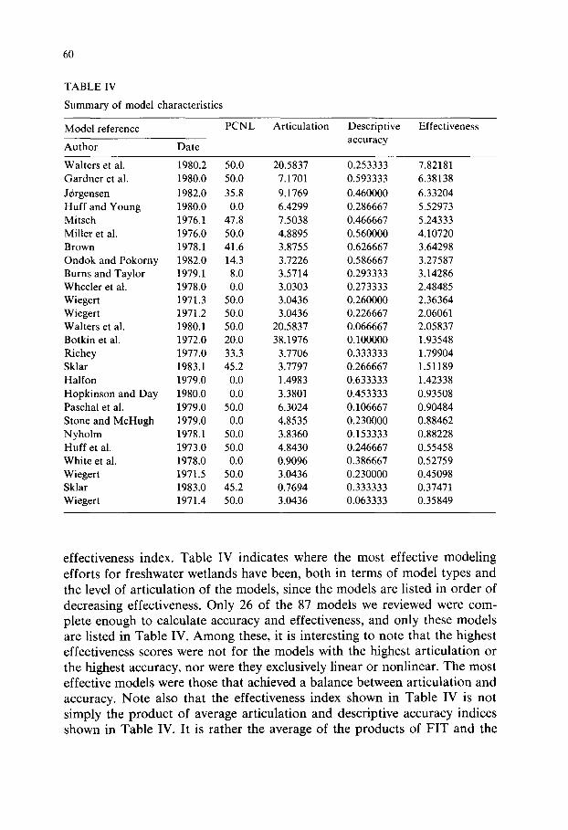


![Scientology Sklar Case 2009 SupremeCt Writ S.Ct.08-9180-Sklar-Cert_Petition[1]](https://static.documents.pub/doc/80x56/577dabcd1a28ab223f8cfa99/scientology-sklar-case-2009-supremect-writ-sct08-9180-sklar-certpetition1.jpg)

