Countergradient heat flux observations during the eveningtransition period
E. Blay-Carreras1, E. R. Pardyjak2, D. Pino1,3, D. C. Alexander2, F. Lohou4, and M. Lothon4
1Department of Applied Physics, Universitat Politècnica de Catalunya, BarcelonaTech, Barcelona, Spain2Department of Mechanical Engineering, University of Utah, Salt Lake City, UT, USA3Institute of Space Studies of Catalonia (IEEC–UPC), Barcelona, Spain4Université de Toulouse – CNRS 5560, Laboratoire d’Aérologie, Toulouse, France
Received: 4 March 2014 – Published in Atmos. Chem. Phys. Discuss.: 21 March 2014Revised: 30 June 2014 – Accepted: 8 July 2014 – Published: 3 September 2014
Abstract. Gradient-based turbulence models generally as-sume that the buoyancy flux ceases to introduce heat into thesurface layer of the atmospheric boundary layer in tempo-ral consonance with the gradient of the local virtual potentialtemperature. Here, we hypothesize that during the eveningtransition a delay exists between the instant when the buoy-ancy flux goes to zero and the time when the local gradientof the virtual potential temperature indicates a sign change.This phenomenon is studied using a range of data collectedover several intensive observational periods (IOPs) duringthe Boundary Layer Late Afternoon and Sunset Turbulencefield campaign conducted in Lannemezan, France. The focusis mainly on the lower part of the surface layer using a towerinstrumented with high-speed temperature and velocity sen-sors.
The results from this work confirm and quantify a flux-gradient delay. Specifically, the observed values of the delayare ∼ 30–80 min. The existence of the delay and its dura-tion can be explained by considering the convective timescaleand the competition of forces associated with the classicalRayleigh–Bénard problem. This combined theory predictsthat the last eddy formed while the sensible heat flux changessign during the evening transition should produce a delay. Itappears that this last eddy is decelerated through the actionof turbulent momentum and thermal diffusivities, and that thedelay is related to the convective turnover timescale. Obser-vations indicate that as horizontal shear becomes more im-portant, the delay time apparently increases to values greaterthan the convective turnover timescale.
1 Introduction
The general behavior of the diurnal cycle of the atmosphericboundary layer (ABL) under clear sky fair weather condi-tions is well-known (Stull, 1988). During the day, a convec-tive boundary layer driven by surface and entrainment fluxesexists (Moeng and Sullivan, 1994; Sorbjan, 1996; Sullivanet al., 1998; Pino et al., 2003; Fedorovich et al., 2001). Latein the afternoon, due to radiative cooling of the ground, astable boundary layer (SBL), where turbulence may be sup-pressed, is created adjacent to earth’s surface (Nieuwstadt,1984; Mahrt, 1998; Beare et al., 2006). A residual layer (RL)of weak turbulence exists above this SBL. The RL occupiesa similar space as the mixed layer of that day’s convectiveboundary layer (CBL). However, the details of certain pro-cesses, particularly those associated with nonstationary tran-sitional periods, are not as well understood. The transitionoccurring after the peak in solar insulation can be dividedinto two distinct periods: theafternoon transition, when thesurface sensible heat flux starts to decrease from its middaymaximum, and theevening transition, when the surface sen-sible heat flux becomes negative (Nadeau et al., 2011).
This paper focuses on the behavior of the buoyancy fluxand temperature gradient in the surface layer during theevening transition period by analyzing measurements ob-tained during the Boundary Layer Late Afternoon and Sun-set Turbulence (BLLAST;Lothon et al., 2014) field cam-paign. BLLAST was conceived to study the late afternoontransition (LAT) processes in the ABL. Objectives of theBLLAST project include gaining a better understanding of
Published by Copernicus Publications on behalf of the European Geosciences Union.
9078 E. Blay-Carreras et al.: Countergradient heat flux observations during the evening transition period
(a) the importance of surface heterogeneity on the LAT and(b) the structure and evolution of the boundary layer itselfduring this period of the day. The team members of thisproject include an international group of scientists from dif-ferent European countries and the USA. The main hypothe-ses to be tested during this study are focused on the after-noon transition; therefore, the observations obtained from theBLLAST campaign provide a valuable framework to developthe present work.
In this work, we hypothesize that during the evening tran-sition, a delay exists between the instant when the buoyancyflux goes to zero and the time when the local gradient of thevirtual potential temperature indicates a sign change. Whilethis hypothesis has received little attention during the tran-sition period,Ghan(1981) and Franchitto and Rao(2003)attempted to find a relationship between the temperature gra-dient and the heat flux, considering the complete diurnal cy-cle. In addition, nonlocal modeling studies have been used todevelop different theories about eddy diffusivity and coun-tergradient transport (Deardorff, 1972; Holtslag and Moeng,1991). Holtslag and Boville(1993) introduced a nonlocalterm in the parameterization of vertical diffusion in the atmo-spheric boundary layer to account for convective situationswhere the heat flux can be counter to the local potential tem-perature gradient (positive heat flux and positive gradient ofpotential temperature). In this case, turbulence results fromnonlocal transport by eddies on the order of the size of theboundary layer. This mainly occurs at the upper part of theboundary layer, just below the entrainment zone and far fromthe surface layer.
Investigations using observations (Grimsdell andAngevine, 2002) or large-eddy simulations (Nieuwstadtand Brost, 1986; Sorbjan, 1997; Pino et al., 2006) haveshown that entrainment fluxes introduce heat in the bound-ary layer after the sensible heat flux becomes negative,producing turbulence in the middle of the mixed layerseveral hours after sunset (demixing process). However,Darbieu et al. (2014) have recently shown, using LES(large-eddy simulations) and aircraft observations during theafternoon transition, that turbulence (TKE and variances)decreases earlier in the upper levels of the boundary layer.If this result is also true during the evening transition, itseems that demixing, if it exists, cannot also be attributedto entrainment. Again, none of these studies focused on theresponse of the surface layer during this transition.
At the surface layer, it is normally assumed that the buoy-ancy flux ceases to introduce heat into the ABL at the sameinstant that the gradient of the virtual potential temperaturereflects this phenomenon. Most simulation models work us-ing this basic concept. A good knowledge of the phenomenonand evolution of the afternoon/evening transition is crucialfor developing more realistic models and creating better ap-proximations (Sorbjan, 1997; Cole and Fernando, 1998; Ed-wards et al., 2006; Pino et al., 2006; Angevine, 2007; Nadeauet al., 2011).
The objective of this article is to investigate this phe-nomenon using a range of data collected over several days,focusing mainly on the lower surface layer, using a tower in-strumented with fast response fine-wire (FW) thermocouplesand sonic anemometers/thermometers (SATs). Moreover, thehypothesis will be supported by theories that can explain thisphenomenon, such as the inverse Bénard problem, the effectof convective time or the definition of convection character-istics with the help of the Monin–Obukhov length scale.
The paper is structured as follows. In Sect. 2, we presentthe theory supporting the main hypothesis of the article.In Sect. 3, we describe the BLLAST field campaign andthe instruments selected to test the hypothesis including themethod for identifying time periods of interest for the anal-ysis. In Sect. 4, we present the results focusing on the delayand convective time analysis, the Monin–Obukhov length-scale analysis and turbulent Rayleigh number analysis. Fi-nally, Sect. 5 summarizes the results.
2 Background theory
The hypothesis, which was described in the introduction, canbe related to the well-known Rayleigh–Bénard (R–B) prob-lem (thermal instability) associated with the heating of a qui-escent layer of fluid from below, which ultimately resultsin turbulent free convection (Kundu and Cohen, 2010). Thestandard R–B problem is based on the idea that there is alayer of fluid heated from below, however, the upper partof the layer is heavy enough to stifle the convective move-ments. Both viscosity and thermal diffusivity make it difficultfor convection movements to happen. Therefore, large tem-perature gradients are required to create the instability thatmakes movement possible. Here we consider similar physics,but in the opposite sense because during LAT the CBL iscooled from below. The idea was previously introduced andexperimentally studied byCole and Fernando(1998), whodesigned a laboratory water tank experiment to observe thedecay of temperature and velocity fluctuations in the CBL inresponse to cooling the surface.
In both the classical R–B problem and the phenomenastudied in this paper, a delay exists that is related with thebuoyancy flux at the surface and convective movements.When the buoyancy flux ceases, the convective movementscontinue for some time. This delay can be similarly producedfrom the same factors that drive the classical R–B problem.In other words, the viscosity and the thermal diffusivity makeit possible for this transition to happen in a smoother way.The dimensionless parameter, which compares the destabi-lizing forces (buoyancy forces) with the stabilizing forces(viscosity and thermal diffusivity) is the Rayleigh number,
E. Blay-Carreras et al.: Countergradient heat flux observations during the evening transition period 9079
whereg is the gravitational constant,1θv is the average vir-tual potential temperature difference over the layer depth1z
(taken here as the height of the atmospheric near-surfacelayer), κ is the molecular thermal diffusivity andν is themolecular kinematic viscosity. For the classical R–B problemwith heating from below, when the Rayleigh number reachesa critical value,Racr, convective movement will start. In thispaper, we provide preliminary evidence for a transitional tur-bulent Rayleigh number at which convective motions cease.
3 Methodology
This study was performed within the framework of theBLLAST field campaign. Amongst the wide range of in-struments deployed during the campaign, a relatively short(10 m), but highly instrumented tower was selected to beused in this study. This tower, located at 43◦07′39.3′′ N,00◦21′57.9′′ E was selected because it was equipped with alarge number of closely spaced sensors, and was placed overrelatively simple and homogeneous terrain (flat grass field).The sensors deployed on the tower included SATs and FWs.The instrument-deployment strategy focused many sensorsclose to the ground in order to observe small and fast changesconnected to this zone. Figure1a shows the vertical locationof the instruments on the 10 m mast and Fig.1b shows anaerial view of the site where the tower was located.
Four Campbell Scientific sonic anemometer thermometers(CSAT3, Logan, UT) fitted with 12.7 µm diameter CampbellScientific E-TYPE model FW05 fine-wire thermocoupleswere mounted at the following heights: 2.23, 3.23, 5.27 and8.22 m above ground. Closer to the ground, there were fouradditional FW05 sensors mounted at 0.091, 0.131, 0.191, and0.569 m above ground. These small diameter thermocoupleswere selected to minimize solar loading and response timeto turbulent temperature fluctuations. The lowest sensor wasplaced just in the grass canopy. The grass around this sen-sor was regularly trimmed to maintain a canopy height ofapproximately 7–9 cm. During the intensive observation pe-riods (IOPs) the lowest FWs were installed during the af-ternoon through the entire transition period to provide anexpanded data set. All instruments recorded data at 20 Hz.However, 5 min block-averaged data are presented in theanalysis shown below. All data were processed using the soft-ware package ECPACK (Van Dijk et al., 1998).
This study focuses on the analysis of the following groupof IOP days during the BLLAST campaign: 24, 25, 27, 30June and 1, 2 July 2011. These IOPs represent days when the10 m tower was completely instrumented. Table 1 summa-rizes the information used to characterize the IOPs includingthe daily maximum surface sensible heat flux, the duration ofthe diurnal cycle and the days since the last rainfall.
The primary goal of this work is to characterize and under-stand the observed time delay between the instant when thebuoyancy flux is zero and when the virtual potential temper-
Figure 1. (a) Sketch of the distribution of sensors that were de-ployed on the 10 m mast during BLLAST and(b) an aerial view ofthe site (the red X indicates the location of the 10 m tower).
ature gradient changes sign. To sketch the change of sign ofthe gradient of virtual potential temperature, Fig.2 shows thetemporal evolution of the vertical profile of potential temper-ature measured by the FWs located on the 10 m mast duringthe evening of 1 July 2011. We can observe how, at the low-est levels, the gradient of potential temperature changes signfrom negative to positive.
The instrumentation used in the campaign included fewerSATs than FW thermocouples, so the instruments were notalways collocated. However, to include the effects of humid-ity, we use the measurements made by the SATs located at2.23 and 3.23 m because these are the lowest sensors whichcan be used to simultaneously measure virtual potential tem-perature gradients and buoyancy flux.
9080 E. Blay-Carreras et al.: Countergradient heat flux observations during the evening transition period
Table 1.Based on the observations taken during the BLLAST campaign, IOP day, maximum sensible heat flux (SHmax) , length of the day,days since last rainfall, delay time, convective timescale, convective intensity, transitional turbulent Rayleigh number and temporal differencebetween the time whenRa and buoyancy flux change sign.
Day SHmax Diurnal cycle Sunset Days since DT t∗ −z/L Convective Rat Rat–BF(IOP) (Wm−2) (h) (UTC) last rainfall (min) (min) intensity (min)
Figure 2.Observed 5 min averaged vertical profile of potential tem-perature during the evening transition on 1 July 2011.
To estimate the virtual potential temperature (θv), we as-sumed that the virtual temperature (Tv) can be approximatedby the sonic temperature. The virtual potential temperaturewas then estimated using the adiabatic lapse rate (0) as fol-lows: θv = Tv + 0z. Gradients were then computed using fi-nite differences (Chapra and Canale, 1998).
The following paragraphs describe how this delay is deter-mined. Figure3 shows the observed temporal evolution ofθvat 2.23 and 3.23 m during two IOPs and illustrates the timewhen the change in sign of the gradient between the virtualpotential temperature at the two levels occurs. The change insign of the gradient first occurs at 18:36 UTC (coordinateduniversal time) on 30 June 2011 and at 18:51 UTC on 1 July2011. The buoyancy flux (BF) was computed as
BF =g
Tvw′θ ′
v. (2)
Here, w′θ ′v is the vertical kinematic flux of virtual poten-
tial temperature. The lowest sensor (2.23 m) is used to de-fine when the buoyancy flux ceases. In other words, whenthere is no more heat coming from the ground being mea-
17.5 18 18.5 19295
295.5
296
296.5
297
297.5
Time (UTC)
θv(K
)
a
2.23m SAT
3.23m SAT
17.5 18 18.5 19297.5
298
298.5
299
299.5
300
Time (UTC)
θv(K
)
b
2.23m SAT
3.23m SAT
( )
( )
Figure 3. Observed temporal evolution of the virtual potential tem-perature at 2.23 m (solid line) and 3.23 m (dashed line) during theevening transitions on(a) 30 June and(b) 1 July 2011.
sured at that probe. For instance, on 30 June and on 1 July2011 the lower sensor shows that the flux ceases at approx-imately 18:18 and 17:54 UTC, respectively. The delay timebetween when temperature gradient and buoyancy flux passthrough zero is then simply the difference between the twotimes.
E. Blay-Carreras et al.: Countergradient heat flux observations during the evening transition period 9081
17 17.5 18 18.5 19 19.524−Jun−2011
25−Jun−2011
26−Jun−2011
27−Jun−2011
28−Jun−2011
29−Jun−2011
30−Jun−2011
01−Jul−2011
02−Jul−2011
Time (UTC)
BFGrad.ev
Figure 4. For each IOP, instant when buoyancy flux (bullets) andvirtual potential temperature gradient (triangles) change sign.
To develop the theory for the inverse R–B problem, thearea selected is the lowest surface layer specifically from2.23 to 8.2 m, which is the area with an evolution closer tothe idea proposed by Bénard. First, we calculate the turbulentthermal diffusivity (KH ) and the turbulent viscosity (KM ).These two parameters can be estimated using the followingequations.
KH = w′θ ′v/
∂θv
∂z, (3)
KM = −u2∗/
∂S
∂z, (4)
whereu∗ is the friction velocity andS is the mean windspeed. There is relatively little variability in these parame-ters during the day; therefore, they are estimated by usingthe maximum buoyancy flux to avoid possible influences ofthe skin flow close to the afternoon transition and to be con-sistent during all IOPs.
4 Results and discussion
4.1 Delay time analysis
Using the procedure described above, the delay time (DT)was computed for all IOPs. The results for all the studiedIOPs are summarized in Fig.4, where the instants when thebuoyancy flux and the virtual potential temperature gradientchange sign are shown. As is shown in the figure, this de-lay was present on all days analyzed. The delay varies fromaround 30 to 80 min. The numerical values for the delay timefor all IOPs are given in Table1.
A possible explanation for the occurrence of this delaycan be related to eddy movements associated with warmair plumes that form at the surface. The moment that the
buoyancy flux transitions from positive to negative valuesindicates that no more heat is being introduced to the at-mosphere from the ground. Additionally, the upward move-ment due to warming of the air next to the ground (formationof new thermal plumes) also stops. However, these move-ments are not instantaneous movements. Quite the opposite,these movements start at the ground, mix through the sur-face layer and potentially move upward, crossing the entireboundary layer up to the entrainment zone and then descendwith the warm air introduced by the overshoots of the ed-dies in the free atmosphere (i.e., the movements act over aneddy turnover period of time). When the introduction of heatstops (BF= 0 W m−2), the last eddy forms and continues tomove through the boundary layer. During this eddy turnovertime period, the surface layer cools, changing the sign of thetemperature gradient. Consequently, the surface layer doesnot instantaneously respond when the surface flux stops, be-cause the mixing (and heat transfer) continues during oneeddy turnover time. This idea has been presented in differentstudies, for instance bySorbjan(1997), although it focusesmainly on movements in the entrainment zone and not at theground. Further, this hypothesis also is compatible with theexistence of a neutral layer above the decoupled stable sur-face layer, where, due to entrainment, turbulence may stillexist (Nieuwstadt and Brost, 1986; Grimsdell and Angevine,2002; Pino et al., 2006).
An analysis of the dimensionless temperature gradient(φh), as described by the Monin–Obukhov similarity the-ory (MOST), was used to investigate the presence of thisdelay. Theoretically, the Monin–Obukhov length scale (L)should include the effects associated with synoptic-scale mo-tion (Stull, 1988). L can be used as a scaling parameter to de-fine the convective characteristics of the atmospheric bound-ary layer. Using this parameter, the effects of buoyancy andmechanical production of turbulence can be compared at aspecific altitude. The surface layer scaling parameter (−z/L)provides a metric indicating the strength of the convectiveconditions during the IOP period leading into the eveningtransition. We computedφh and−z/L as follows:
φh =kz
θSLv∗
∂θv
∂z=
kzu∗
−w′θ ′v
∂θv
∂z, (5)
−z
L=
kzg(w′θ ′
v
)s
θvu3∗
. (6)
wherek is the von Karman constant, andz is the analysisaltitude (2.23 m).
Figure5 shows every 5 minφh as a function of−z/L at2.23 m for 30 June and 1 July 2011. Clearly, there are pointswhich break away from MOST (indicated by the dashedblack line). Specifically, gradient theory fails locally due tothe countergradient observations that appear in the plots dur-ing near stable conditions. Formally, MOST should be validin the stable layer. However, during the transition period, one
9082 E. Blay-Carreras et al.: Countergradient heat flux observations during the evening transition period
( ) ( )
Figure 5. Dimensionless temperature gradient (φh) as a function of−z/L at 2.23 m on(a) 30 June and(b) 1 July 2011. Dashed line isthe approximation ofBusinger et al.(1971).
can observe that the log surface layer locally disappears closeto the ground as there is a decoupling between the old log-layer and the newly forming stable layer, as shown in thetransitioning temperature profile in Fig.2. In the past, thisphenomenon was mainly observed for the air–sea boundarylayer (Sahlee et al., 2008). However,Smedman et al.(2007)also observed this behavior at a site over land, but for atmo-spheric conditions that were quite different from our studycase. In particular, their case was for strong winds between 7and 10 m s−1 in contrast with BLLAST’s calm conditions.
4.2 Convective time analysis
To provide support for our delay hypothesis, the convectivetimescale is analyzed and compared to the delay timescale.The convective timescale can be defined as the approximatetime that it takes one eddy to traverse the atmospheric bound-ary layer. The hypothesis described above should be sup-ported if the value of the delay and the value of the convectivetime are similar. In other words, the delay exists as a resultof the continued movement of the boundary layer due to thelast eddy motions generated at the surface.
It should be noted that there is debate in the researchcommunity regarding the use of various timescales dur-ing the transition period. There is not a general agree-ment about which scaling time is the best option during theafternoon/evening transition (Nieuwstadt and Brost, 1986;Lothon et al., 2014). However, it will be used to learn moreabout the theory proposed.
First, the convective timescale (t∗) is computed followingDeardorff(1972):
t∗ =zi
w∗
, wherew∗ =
[gzi
θvw′θ ′
v
] 13
(7)
being zi the boundary-layer depth. These scales are thencomputed averaging the 5 min periods just before the buoy-ancy flux vanishes. The depth of the boundary layer was ob-tained from the BLLAST campaign’s UHF (ultra-high fre-quency) profiler, which was installed approximately 150 maway from the 10 m tower. Specifically, we estimate theheight of the ABL from the local maxima of the refractiveindex structure coefficient (Lothon et al., 2014).
The results from the calculation of the convectivetimescale for all IOPs are shown in Table1 and Fig.6. Itis clear that the delay time and the convective time comparebetter on some IOPs than others. For some IOPs, such as24 and 30 June 2011, the delay time is nearly the same asthe convective time. However, on other days, such as 25 or27 June, the convective scale and delay time compare quitepoorly.
These observed differences between the timescales couldbe a result of the characteristics of the boundary layer as-sociated with the different IOPs that are not accounted forin the assumptions associated with the convective timescale.In other words, IOPs associated with very convective condi-tions seem to follow the theory better, while more synopti-cally forced conditions fail.
4.3 Monin–Obukhov length analysis
In contrast to Sect. 4.1, here we computed a characteristic−z/L for each of the IOPs by averaging it over the timeperiod prior to the main afternoon transition (from 12:00 to16:45 UTC). From the results, we observe that each IOP canbe classified as a convective or weakly convective day (seeTable 1). The most convective IOPs were 24 and 30 June2011. These IOPs were also those with a better correlationbetween the delay time and the convective timescale (seeFig. 6 and Table1). However, the weaker convective days(i.e., 25 and 27 June 2011) show a larger difference betweenthe delay and convective times (see Table1). Less-convectivedays have higher values ofu∗ as a result of increased me-chanical turbulence production close to the ground (2.23 m).On these weakly convective days, the delay time is increasedas shear prevents the rapid onset of a stable boundary layerat the surface.
E. Blay-Carreras et al.: Countergradient heat flux observations during the evening transition period 9083
20
30
40
50
60
70
80
90
IOP days
Tim
e(m
in)
24−Ju
n−2011
25−Ju
n−2011
26−Ju
n−2011
27−Ju
n−2011
28−Ju
n−2011
29−Ju
n−2011
30−Ju
n−2011
01−Ju
l−2011
02−Ju
l−2011
DT
t*
Figure 6. For each IOP, delay (asterisks) and convective (triangles)times.
Figure7 shows the difference between the two timescalesas a function of−z/L. Evidently, the BLLAST data indi-cate an exponentially decreasing relationship between thetimescale and the Monin–Obukhov parameter. This relation-ship is likely to be a function of local effects and should be in-vestigated at other sites to see if a general relationship can beascertained. Regardless, Fig.7 shows a potentially site spe-cific method for forecasting the delay time using midday datafrom a single flux tower.
4.4 Turbulent Rayleigh number analysis
The turbulent Rayleigh number (Raturb) can be used to ex-plain the behavior of the delay time. It is calculated withEq. (1) but, instead of using molecular thermal diffusivity (κ)and molecular kinematic viscosity (ν), we use the turbulentthermal diffusivity (see Eq. 3) and turbulent viscosity (seeEq. 4). Therefore,Raturb reads
Raturb =g
θv
1θv(1z)3
KH KM
, (8)
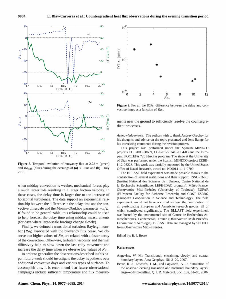
where1z is the distance between the sensors (8.2–2.23 m).We select these two sensors because this area has an evo-lution closer to the idea proposed by Bénard. Turbulent ther-mal diffusivity and turbulent viscosity could play a role in theinitiation or the ceasing of convection. We define the transi-tional turbulent Rayleigh number (Rat) as the value ofRaturbwhen the buoyancy flux ceases. Figure8 shows the tem-poral evolution of buoyancy flux andRaturb from 17:00 to20:00 UTC on 30 June and 1 July 2011. As can be observed,Raturb becomes negative later on 1 July 2011 similarly to thechanges in sign of the local virtual potential temperature gra-dient. For all the analyzed days, BF is negative several tens
0.1 0.15 0.2 0.25 0.3 0.35100
101
102
−z/L
DT-t
∗(m
in)
Figure 7. For all the IOPs, difference between the delay and con-vective times as a function of−z/L.
of minutes beforeRaturb. Table 1 shows this temporal differ-ence and the value ofRat. As can be observed, this temporaldifference is clearly related with DT being larger on dayswith a larger temporal difference betweenRat and BF.
We assume that, on each day,Rat is in correspondencewith the critical Rayleigh number (Racr). It is important tonotice that during the early morning of days with large val-ues ofRacr, larger values of buoyancy flux are needed to on-set convection. Additionally, during the evening transition onthese days, convection stops quickly when the buoyancy fluxceases. By assumingRat ∝ Racr, larger values ofRat haveto be observed on these days. Figure9 shows DT− t∗ as afunction ofRat for all the studied days. There is an exponen-tially decreasing relationship between both parameters. IOPswith largerRat have a smaller difference between convectiveand delay times, meaning convection stops quickly. On thecontrary, on days with low values ofRat convection sloweddown smoothly, increasing the delay time and consequentlyDT − t∗.
5 Conclusions
It has been shown that there is a clear failure of flux gra-dient theory during the evening transition period as a resultof nonlocal processes. Analysis of the data obtained from a10 m tower during the BLLAST campaign indicates that atime delay exists between the time when the buoyancy fluxceases and the change in sign of the vertical gradient of thevirtual potential temperature. This was the case for all IOPs.
For strong-to-moderate convective days, the delay time isrelatively short (∼ 30–40 min) and corresponds closely to thetimescale associated with the last eddy movements. In otherwords, it is similar to the convective timescale. However,
9084 E. Blay-Carreras et al.: Countergradient heat flux observations during the evening transition period
Figure 8. Temporal evolution of buoyancy flux at 2.23 m (green)andRaturb (blue) during the evenings of(a) 30 June and(b) 1 July2011.
when midday convection is weaker, mechanical forces playa much larger role resulting in a larger friction velocity. Inthese cases, the delay time is larger due to the increase ofhorizontal turbulence. The data support an exponential rela-tionship between the difference in the delay time and the con-vective timescale and the Monin–Obukhov parameter−z/L.If found to be generalizable, this relationship could be usedto help forecast the delay time using midday measurements(for days where large-scale forcings change slowly).
Finally, we defined a transitional turbulent Rayleigh num-ber (Rat) associated with the buoyancy flux cease. We ob-serve that higher values ofRat are related with a faster decayof the convection. Otherwise, turbulent viscosity and thermaldiffusivity help to slow down the last eddy movement andincrease the delay time when we observe low values ofRat.
In order to generalize the observations described in this pa-per, future work should investigate the delay hypothesis overadditional convective days and various types of surfaces. Toaccomplish this, it is recommend that future observationalcampaigns include sufficient temperature and flux measure-
0 2 4 6 8 10 12100
101
102
Rat
DT-t
∗(m
in)
Figure 9. For all the IOPs, difference between the delay and con-vective times as a function ofRat.
ments near the ground to sufficiently resolve the countergra-dient processes.
Acknowledgements.The authors wish to thank Andrey Grachev forhis thoughts and advice on the topic presented and Jens Bange forhis interesting comments during the revision process.
This project was performed under the Spanish MINECOprojects CGL2009-08609, CGL2012-37416-C04-03 and the Euro-pean POCTEFA 720 FluxPyr program. The stage at the Universityof Utah was performed under the Spanish MINECO project EEBB-I-12-05228. This work was partially supported by the United StatesOffice of Naval Research, award no. N00014-11-1-0709.
The BLLAST field experiment was made possible thanks to thecontribution of several institutions and their support: INSU-CNRS(Institut National des Sciences de l’Univers, Centre National dela Recherche Scientifique, LEFE-IDAO program), Météo-France,Observatoire Midi-Pirénées (University of Toulouse), EUFAR(EUropean Facility for Airborne Research) and COST ES0802(European Cooperation in Science and Technology). The fieldexperiment would not have occurred without the contribution ofall participating European and American research groups, all ofwhich contributed significantly. The BLLAST field experimentwas hosted by the instrumented site of Centre de Recherches At-mosphériques, Lannemezan, France (Observatoire Midi-Pirénées,Laboratoire d’Aérologie). BLLAST data are managed by SEDOO,from Observatoire Midi-Pirénées.
Edited by: R. J. Beare
References
Angevine, W. M.: Transitional, entraining, cloudy, and coastalboundary layers, Acta Geophys., 56, 2–20, 2007.
Beare, R. J., Edwards, J. M., and Lapworth, A. J.: Simulation ofthe observed evening transition and nocturnal boundary layers:large–eddy modelling, Q. J. R. Meteorol. Soc., 132, 61–80, 2006.
E. Blay-Carreras et al.: Countergradient heat flux observations during the evening transition period 9085
Businger, J. A., Wyngaard, J. C., Izumi, Y., and Bradley, E. F.: Flux-Profile Relationships in the Atmospheric Surface Layer, J. At-mos. Sci., 28, 181–189, 1971.
Chapra, S. C. and Canale, R. P.: Numerical Methods for Engineers,Boston, McGraw-Hill Companies, 3 edn., 1998.
Cole, G. S. and Fernando, H. J. S.: Some aspects of the decay ofconvective turbulence, Fluid. Dyn. Res., 23, 161–176, 1998.
Darbieu, C., Lohou, F., Lothon, M., Couvreux, F., Pino, D., Durand,P., Blay-Carreras, E., and Vilà-Guerau de Arellano, J.: Evolutionof the turbulence during the afternoon transition of the convec-tive boundary layer: a spectral analysis, J. 21st Symposium onBoundary Layer and Turbulence, 8–13 June 2014, Leeds (UK),2014.
Deardorff, J.: Numerical Investigation of Neutral and UnstablePlanetary Boundary Layers, J. Atmos. Sci., 7, 91–115, 1972.
Edwards, J. M., Beare, R. J., and Lapworth, A. J.: Simulation ofthe observed evening transition and nocturnal boundary layers:Single-column modelling, Q. J. Roy. Meteorol. Soc., 132, 61–80, 2006.
Fedorovich, E., Nieuwstadt, F. T. M., and Kaiser, R.: Numerical andlaboratory study of horizontally evolving convective boundarylayer. Part II: Effects of elevated wind shear and surface rough-ness, J. Atmos. Sci., 58, 546–560, 2001.
Franchitto, S. H. and Rao, V. B.: The correlation between temper-ature gradient and eddy heat flux in the northern and southernhemispheres, J. Meteorol. Soc. Jpn. Ser. II, 81, 163–168, 2003.
Ghan, S. J.: Modelling the synoptic scale relationship between eddyheat flux and the meridional temperature gradient, MassachusettsInstitute of Technology (MIT), Cambridge, Massachusetts, USA,1981.
Grimsdell, A. W. and Angevine, W. M.: Observations of the after-noon transition of the convective boundary layer, J. Appl. Mete-orol., 41, 3–11, 2002.
Haeffelin, M., Angelini, F., Morille, Y., Martucci, G., Frey, S.,Gobbi, G. P., Lolli, S., O’Dowd, C. D., Sauvage, L., Xueref-Rémy, I., Wastine, B., and Feist, D. G.: Evaluation of mixing-height retrievals from automatic profiling lidars and ceilometersin view of future integrated networks in europe, Bound.-Lay. Me-teorol., 143, 49–75, 2012.
Holtslag, A. A. M. and Moeng, C.: Eddy diffusivity and countergra-dient transport in the convective atmospheric boundary layer, J.Atmos. Sci., 48, 1690–1698, 1991.
Holtslag, A. A. M. and Moeng, C.: Local versus nonlocal boundary-layer diffusion in a global climate model, J. Climate, 6, 1825–1842, 1991.
Kundu, P. J. and Cohen, I. M.: Fluid Mechanics, Academic Press,Waltham (MA), USA, 904 pp., 2010.
Lothon, M. and Lenschow, D.: Studying the afternoon transitionof the planetary boundary layer, Eos Trans. AGU, 91, 253–260,2010.
Lothon, M., Lohou, F., Pino, D., Couvreux, F., Pardyjak, E. R.,Reuder, J., Vilà-Guerau de Arellano, J., Durand, P., Hartogen-sis, O., Legain, D., Augustin, P., Gioli, B., Faloona, I., Yagüe,C., Alexander, D. C., Angevine, W. M., Bargain, E., Barrié,J., Bazile, E., Bezombes, Y., Blay-Carreras, E., van de Boer,A., Boichard, J. L., Bourdon, A., Butet, A., Campistron, B., deCoster, O., Cuxart, J., Dabas, A., Darbieu, C., Deboudt, K., Del-barre, H., Derrien, S., Flament, P., Fourmentin, M., Garai, A.,Gibert, F., Graf, A., Groebner, J., Guichard, F., Jimenez Cortes,
M. A., Jonassen, M., van den Kroonenberg, A., Lenschow, D. H.,Magliulo, V., Martin, S., Martinez, D., Mastrorillo, L., Moene,A. F., Molinos, F., Moulin, E., Pietersen, H. P., Piguet, B., Pique,E., Román-Cascón, C., Rufin-Soler, C., Saïd, F., Sastre-Marugán,M., Seity, Y., Steeneveld, G. J., Toscano, P., Traullé, O., Tzanos,D., Wacker, S., Wildmann, N., and Zaldei, A.: The BLLASTfield experiment: Boundary-Layer Late Afternoon and SunsetTurbulence, Atmos. Chem. Phys. Discuss., 14, 10789–10852,doi:10.5194/acpd-14-10789-2014, 2014.
Moeng, C.-H. and Sullivan, P. P.: A comparison of shear- andbuoyancy-driven planetary boundary layer flows, J. Atmos. Sci.,51, 999–1022, 1994.
Nadeau, D. F., Pardyjak, E. R., Higgins, C. W., Fernando, H. J. S.,and Parlange, M. B.: A simple model for the afternoon and earlyevening decay of convective turbulence over different land sur-faces, Bound.-Lay. Meteorol., 141, 301–324, 2011.
Nieuwstadt, F. T. M.: The turbulent structure of the stable, nocturnalboundary layer, J. Atmos. Sci., 41, 2202–2216, 1984.
Nieuwstadt, F. T. M. and Brost, R. A.: The decay of convective tur-bulence, J. Atmos. Sci., 43, 532–546, 1986.
Pino, D., Vilà-Guerau de Arellano, J., and Duynkerke, P. G.: Thecontribution of shear to the evolution of a convective boundarylayer, J. Atmos. Sci., 60, 1913–1926, 2003.
Pino, D., Jonker, H. J. J., Vilà-Guerau de Arellano, J., and Dosio, A.:Role of shear and the inversion strength during sunset turbulenceover land: Characteristic length scales, Bound.-Lay. Meteorol.,121, 537–556, 2006.
Sahlée, E., Smedman, A., Rutgersson, A., and Högström, U.: Influ-ence of a new turbulence regime on the global air-sea heat fluxes,J. Climate, 121, 5925–5941, 2007.
Smedman, A., Högström, U., Hunt, J. C. R., and Sahlée, E.:Heat/mass transfer in the slightly unstable atmospheric surfacelayer, Q. J. Roy. Meteorol. Soc., 133, 37–51, 2007.
Sorbjan, Z.: Effects caused by varying the strength of the cappinginversion based on a large eddy simulation model of the shear-free convective boundary layer, J. Atmos. Sci., 53, 2015–2024,1996.
Stull, R. B.: An introduction to boundary layer meteorology, D. Rei-del Publ. Comp., Dordrecht, The Netherlands, 670 pp., 1988.
Sullivan, P. P., Moeng, C.-H., Stevens, B., Lenschow, D. H., andMayor, S. D.: Structure of the entrainment zone capping the con-vective atmospheric boundary layer, J. Atmos. Sci., 55, 3042–3064, 1998.
Van Dijk, A., Moene, A. F., and De Bruin, H. A. R.: The princi-ples of surface flux physics: theory, practice and description ofthe ECPACK library, Internal Report 2004/1, Meteorology andAir Quality Group, Wageningen University, Wageningen, TheNetherlands, 99 pp., 2004.
van Driel, R. and Jonker, H. J. J.: Convective Boundary LayersDriven by Nonstationary Surface Heat Fluxes, J. Atmos. Sci., 68,727–738, 2011.


![Error and Uncertainty Quantification in the Numerical ...€¦ · whenever the numerical flux satisfies the system extension of Osher’s famous “E-flux” condition [v]x+ x](https://static.documents.pub/doc/80x56/609e9124d937143e6073718a/error-and-uncertainty-quantification-in-the-numerical-whenever-the-numerical.jpg)


