CO P A U L S C H E R R E R I N S T I T U T CH9900045 PSI Bericht Nr. 99-07 September 1999 ISSN 1019-0643 Waste Management Laboratory Coupled Transport Phenomena in the Opalinus Clay: Implications for Radionuclide Transport Josep M. Soler 30-49 Paul Scherrer Institut CH - 5232 Villigen PSI Telefon 056 310 21 11 Telefax 056 310 21 99
Transcript
CO P A U L S C H E R R E R I N S T I T U T
CH9900045
PSI Bericht Nr. 99-07September 1999ISSN 1019-0643
Waste Management Laboratory
Coupled Transport Phenomena in the Opalinus Clay:Implications for Radionuclide Transport
Coupled Transport Phenomena in the Opalinus Clay:Implications for Radionuclide Transport
Josep M. Soler
PREFACE
The Waste Management Laboratory at the Paul Scherrer Institute is performingwork to develop and test models as well as to acquire specific data relevant toperformance assessments of Swiss nuclear waste repositories. Theseinvestigations are undertaken in close co-operation with, and with the partialfinancial support of, the National Cooperative for the Disposal of RadioactiveWaste (Nagra). The present report is issued simultaneously as a PSI-Berichtand a Nagra Technical Report.
PSI Bericht 99-07
ABSTRACT
Coupled phenomena (thermal and chemical osmosis, hyperfiltration, coupleddiffusion, thermal diffusion, thermal filtration, Dufour effect) may play animportant role in fluid, solute and heat transport in clay-rich formations, such asthe Opalinus Clay (OPA), which are being considered as potential hosts forradioactive waste repositories. In this study, the potential effects of coupledphenomena on radionuclide transport in the vicinity of a repository for vitrifiedhigh-level radioactive waste (HLW) and spent nuclear fuel (SF) hosted by theOpalinus Clay, at times equal to or greater than the expected lifetime of thewaste canisters (about 1000 years), have been addressed.
Firstly, estimates of the solute fluxes associated with chemical osmosis,hyperfiltration, thermal diffusion and thermal osmosis have been calculated.Available experimental data concerning coupled transport phenomena incompacted clays, and the hydrogeological and geochemical conditions to whichthe Opalinus Clay is subject, have been used for these estimates. Theseestimates suggest that thermal osmosis is the only coupled transportmechanism that could have a strong impact on solute and fluid transport in thevicinity of the repository.
Secondly, estimates of the heat fluxes associated with thermal filtration and theDufour effect in the vicinity of the repository have been calculated. Thecalculated heat fluxes are absolutely negligible compared to the heat fluxcaused by thermal conduction.
As a further step to obtain additional insight into the effects of coupledphenomena on solute transport, the solute fluxes associated with advection,chemical diffusion, thermal and chemical osmosis, hyperfiltration and thermaldiffusion have been incorporated into a simple one-dimensional transportequation. The analytical solution of this equation, with appropriate parameters,shows again that thermal osmosis is the only coupled transport mechanism thatcould have a strong effect on repository performance, in agreement with theprevious estimates.
Finally, the results of two- and three-dimensional simple flow modelsincorporating advection (Darcy's law) and thermal osmosis show that, under theconditions in the vicinity of the repository at the time scales of interest, theadvective component of flow will oppose and cancel the thermal-osmoticcomponent.
After evaluating the different coupled transport mechanisms, the conclusion isthat coupled phenomena will only have a very minor impact on radionuclidetransport in the Opalinus Clay, at least under the conditions at times equal to orgreater than the expected lifetime of the waste canisters (about 1000 years).
PSI Bericht 99-07
ZUSAMMENFASSUNG
Gekoppelte Prozesse (thermische und chemische Osmose, Hyperfiltration,gekoppelte Diffusion, thermische Diffusion, thermische Filtration, Dufour-Effekt)können eine wichtige Rolle spielen beim Transport von Wasser,Wasserinhaltsstoffen und Wärme durch tonreiche Formationen, wie z.B. denOpalinuston (OPA), welche als mögliche Wirtsgesteine für eine Endlager fürradioaktive Abfälle angesehen werden. In der vorliegenden Studie werden diemöglichen Auswirkungen der gekoppelten Prozesse auf den Radionuklid-Transport in der Nähe eines im Opalinuston gelegenen Endlagers für verglastehoch-radioaktive Abfälle (HLW) und abgebrannte Brennelemente (SF)angesprochen für Zeiten die gleich oder grosser als die erwartete Lebensdauerder Abfallkanister (ca. 1000 Jahre) sind.
Zuerst wurden die Flüsse für Wasserinhaltsstoffe als Folge von chemischerOsmose, Hyperfiltration, thermischer Diffusion und thermischer Osmoseabgeschätzt. Dazu wurden verfügbare experimentelle Daten bezüglichgekoppelter Transportprozesse in kompaktierten Tonen, unter Berücksichtigungder hydrogeologischen und geochemischen Bedingungen des Opalinustons,verwendet. Diese Abschätzungen legen den Schluss nahe, dass nur diethermische Osmose als einziger der gekoppelten Transportmechanismen einenwesentlichen Einfluss auf den Stofftransport und den Transport von Wasser inder Nähe eines Endlagers haben könnte.
In einem zweiten Schritt wurden Abschätzungen vorgenommen für denWärmefluss in der Nähe eines Endlagers als Folge von thermischer Filtrationund des Dufour-Effekts. Die berechneten Wärmeflüsse sind aber komplettvernachlässigbar zu demjenigen der Wärmeleitung.
Um einen weiteren Einblick in die Auswirkungen der gekoppelten Prozesse aufden Stofftransport zu erhalten, wurden in einem weiteren Schritt die Flüsse alsFolge von Advektion, chemischer Diffusion, thermischer und chemischerOsmose, Hyperfiltration und thermischer Diffusion mittels einer einfachen ein-dimensionalen Transportgleichung berechnet. Die analytische Lösung dieserGleichung, mit geeigneten Parametern, zeigt wiederum und inÜbereinstimmung mit vorangehenden Abschätzungen, dass die thermischeOsmose der einzige gekoppelte Transport-Mechanismus ist, welcher starkeAuswirkungen auf das Systemverhalten eines Endlagers haben könnte.
Schliesslich zeigen die Ergebnisse im Rahmen eines einfachen zwei- und drei-dimensionalen Fliessmodells unter Berücksichtigung von Advektion (Darcy-Gesetz) und thermischer Osmose, dass - unter den Bedingungen, die in derNähe eines Endlagers herrschen - für die interessierenden Zeitskalen, dieadvektive Komponente des Flusses derjenigen der thermischen Osmoseentgegengesetzt ist und diese kompensiert.
Die Auswertung der verschiedenen gekoppelten Transportmechanismen lässtden Schluss zu, dass gekoppelte Prozesse nur einen sehr beschränktenEinfluss auf den Radionuklid-Transport im Opalinuston haben werden, unter
PSI Bericht 99-07
der Bedingung, dass die Zeiten vergleichbar oder grosser sind als die erwarteteLebensdauer der Abfallkanister (ca. 1000 Jahre).
PSI Bericht 99-07 IV
RESUME
Les phenomenes couples (osmose thermique et chimique, hyperfiltration,diffusion couplee, diffusion thermique, filtration thermique et effet Dufour) sontsusceptibles de jouer un role important au niveau des mecanismesd'ecoulement de transport de solutes et de chaleur dans les formations richesen argiles, telles que les argiles a Opalines (OPA). Ces formations sontconsiderees comme des roches d'accueil potentielles pour le confinement desdechets radioactifs. Dans ce travail, les effets potentiels de phenomenescouples sur le transport de radionucleides ont ete etudies au voisinage d'un sited'entreposage, au sein de I'OPA, soit pour dechets vitrifies de type hautementradioactifs (HLW) que pour le combustible nucleaire usage (SF), et considerantdes temps egaux ou posterieurs a la vie prevue des recipients metalliques(environ 1000 ans).
En premier lieu, les flux de solutes associes aux mecanismes d'osmosechimique, d'hyperfiltration, de diffusion thermique, et d'osmose thermique ontete calcules. Ces estimations ont ete obtenues a partir de donneesexperimentales disponibles, relatives aux processus couples de transport dansles argiles compactees, selon les conditions hydrogeologiques etgeochimiques existant dans les argiles a Opalines. Ces resultats suggerent queseul le mecanisme couple de I'osmose thermique peut avoir un effet importantsur le transport de solutes et de fluides aux alentours du depot.
Dans une deuxieme partie, les flux thermiques associes a la filtration thermiqueet a I'effet Dufour ont ete calcules aux alentours du site d'entreposage. Les fluxthermiques obtenus sont negligeables compares a ceux engendres parconduction thermique.
Lors de I'etape suivante, le but a ete d'obtenir des resultats supplementairessur les effets de phenomenes couples sur le transport de masse en solution.Les flux de solutes associes aux mecanismes d'advection, de diffusionchimique, d'osmose thermique et chimique, d'hyperfiltration et de diffusionthermique ont ete decrits a I'aide d'une equation de transportunidimensionnelle. La solution analytique de cette equation, par le biais deparametres appropries, montre que I'osmose thermique est le seul processusde transport susceptible d'avoir un effet marque sur les performances du depot.Ce resultat est en accord avec les estimations precedentes.
Finalement, les resultats de modeles d'ecoulement simples a deux et a troisdimensions decrivant les processus d'advection (loi de Darcy) et d'osmosethermique ont montre que pour les conditions regnant au voisinage du depot etpour les temps d'interet, la composante advective de I'ecoulement s'oppose acelle thermo-osmotique et Pannule.
En conclusion, revaluation des differents mecanismes de transport couples amis en evidence le tres faible impact du couplage sur le transport des
V PSI Bericht 99-07
radionucleides dans les argiles a Opalines, au moins pour les conditionsreignant a des temps egaux ou posterieurs a la vie prevue des recipientsmetalliques (environs 1000 ans).
PSI Bericht 99-07 VI
RESUM
Els fenòmens aparellats de transport (osmosi tèrmica i química, hiperfiltració,difusió aparellada, difusió tèrmica, filtració tèrmica, efecte Dufour) poden tenirun paper important en el transport de fluid, soluts i calor en formacions amb uncontingut alt d'argiles, com per exemple l'Argila Opalinus (OPA). Actualments'està plantejant la possibilitat de construir dipòsits subterranis de residusradioactius en formacions d'aquest tipus. En aquest estudi es tracten elsefectes potencials de fenòmens aparellats sobre el transport de substànciesradioactives en solució prop d'un dipòsit subterrani de residus radioactius d'altnivell vitrificats (HLW) i combustible nuclear usat (SF) situat en l'ArgilaOpalinus, i a escales de temps iguals o superiors a la durada prevista delscontenidors dels residus (aproximadament 1000 anys).
En primer lloc s'han estimat els fluxes de solut associats amb l'osmosi química,hiperfiltració, difusió tèrmica i osmosi tèrmica, utilitzant dades experimentalsdisponibles sobre argiles compactades i les condicions hidrogeològiques igeoquímiques a les que està sotmesa l'Argila Opalinus. Aquestes estimacionssuggereixen que l'osmosi tèrmica és l'únic mecanisme aparellat de transportque pot tenir un efecte significatiu sobre el transport de solut i solució prop deldipòsit subterrani.
En segon lloc s'han estimat els fluxes de calor associats amb la filtració tèrmicai l'efecte Dufour prop del dipòsit subterrani. Els fluxes que s'han calculat sóncompletament negligibles comparats amb el fluxe degut a la conducció tèrmica.
Com un pas més per entendre els efectes dels fenòmens aparellats detransport, els fluxes de solut associats amb l'advecció, difusió química, osmositèrmica i química, hiperfiltració i difusió tèrmica han estat incorporats en unaequació simple de transport unidimensional. La solució analítica d'aquestaequació, fent servir els paràmetres adequats, indica de nou que l'osmositèrmica és l'únic mecanisme aparellat de transport que pot tenir un efecteimportant sobre el funcionament del dipòsit subterrani.
Finalment, els resultats de models simples bidimensionals i tridimensionals defluxe de fluid que inclouen advecció (llei de Darcy) i osmosi tèrmica, mostrenque sota les condicions prop del dipòsit subterrani a les escales de tempsd'interès, el component advectiu del fluxe s'oposa al component d'osmositèrmica i l'anul·la.
Després d'avaluar els diferents mecanismes aparellats de transport, laconclusió és que aquests mecanismes només tindran un efecte molt menorsobre el transport de substàncies radioactives en l'Argila Opalinus, almenys aescales de temps iguals o superiors a la durada prevista dels contenidors delsresidus (aproximadament 1000 anys).
VII PSI Bericht 99-07
TABLE OF CONTENTS
1. INTRODUCTION 1
2. DIRECT AND COUPLED TRANSPORT PHENOMENA 3
3. ESTIMATES OF SOLUTE FLUXES ASSOCIATED WITH COUPLED TRANSPORTPHENOMENA 7
3.1 Formulation of the solute fluxes 73.1.1 Advection 83.1.2 Chemical diffusion 83.1.3 Chemical osmosis 93.1.4 Hyperfiltration 103.1.5 Thermal diffusion 103.1.6 Thermal osmosis 11
3.2 Diffusion coefficients and hydraulic conductivities for the Opalinus Clay 113.2.1 Hydraulic conductivities 113.2.2 Diffusion coefficients 113.2.3K/D, 12
3.3 Chemical diffusion vs. advection 123.3.1 Peclet number 123.3.2 Assume values for concentration gradients 13
3.4 Hyperfiltration 15
3.5 Chemical osmosis 153.5.1 Chemical osmosis vs. advection 153.5.2 Chemical osmosis vs. chemical diffusion 16
3.6 Thermal diffusion 173.6.1 Thermal diffusion vs. advection 173.6.2 Thermal diffusion vs. chemical diffusion 18
3.7 Thermal osmosis 183.7.1 Thermal osmosis vs. advection 193.7.2 Thermal osmosis vs. chemical diffusion 20
4. ESTIMATES OF THE HEAT FLUXES ASSOCIATED WITH THERMAL FILTRATION ANDTHE DUFOUR EFFECT 21
4.1 Thermal filtration 21
4.2 The Dufour effect 22
5. SIMPLE ONE-DIMENSIONAL TRANSPORT SIMULATIONS INCLUDING THERMAL ANDCHEMICAL OSMOSIS, HYPERFILTRATION, AND THERMAL DIFFUSION. 26
5.1 The transport equation 26
PSI Bericht 99-07 VIM
5.2 Simulations 275.2.1 Model parameters 27
5.2.1.1 Hydraulic, temperature, and osmotic pressure head gradients 275.2.1.2 Other parameters 27
5.2.2 Results and discussion 28
6. COUPLING BETWEEN ADVECTION AND THERMAL OSMOSIS: TWO- AND THREE-DIMENSIONAL FLOW CALCULATIONS. 33
6.1 Two-dimensional model 336.1.1 Model formulation 336.1.2 Results and discussion 34
6.1.2.1 Case 1 (T1 =T2 = 298.15 K) 366.1.2.2 Case 2 (T1 = 299.22 K, T2 = 298.08 K) 36
6.2 Three-dimensional model 396.2.1 Model formulation 396.2.2 Results and discussion 40
6.3 Two-dimensional model with temperature-dependent fluid density and viscosity 476.3.1 Model formulation 486.3.2 Results and discussion 49
7. CONCLUSIONS 51
8. ACKNOWLEDGEMENTS 54
9. REFERENCES 55
10. LIST OF SYMBOLS 59
IX PSI Bericht 99-07
LIST OF FIGURES
Figure 1.1: Electrical double layer in a clay pore (after MARINE & FRITZ, 1981) 1
Figure 3.1: Schematic diagram showing Total Dissolved Solids vs. Distance along the Mt. Territunnel. TDS data from GAUTSCHI, ROSS & SCHOLTIS, 1993 (solid circles), andPEARSON et al., 1999 (crosses). Activity of water (H2O) and osmotic pressure head (Ph)are also given for the sample with the highest salinity in OPA, and for two low-salinitysamples above and below OPA. The dashed lines are hypothetical salinity curves. Thevertical lines are only intended to show the boundaries of the different rock units along thetunnel. The orientation of the tunnel is NW-SE, and the rock strata dip at an angle of about45° to the southeast. The thickness of the Opalinus Clay at the Mont Terri tunnel is about140m(THURY, 1997) 14
Figure 5.1: Relative concentration vs. distance at t = 5000 y. The different curves correspond todifferent values of the thermo-osmotic permeability kr Thermal osmosis will only have asignificant effect if kT> 1012 nf/K/s 28
Figure 5.2: Relative concentration vs. distance at f = 5000 y, for (a) hydraulic conductivity Kequal to 1012 m/s, and (b) effective diffusion coefficient Dg equal to 10" m7s. The differentcurves in both plots correspond to different values of the thermo-osmotic permeability kr....3O
Figure 5.3: Relative concentration vs. distance at t = 5000 y, for two different values of the Soretcoefficient (s = 0 and s = 0.1 K'1) 31
Figure 5.4: Relative concentration vs. distance at t = 5000 y, for the case with an osmotic
pressure head gradient [dnh/ck)equal to 10. (a) Results for different values of the
thermo-osmotic permeability kr (b) Results for different values of the osmotic efficiencya , with kT=0 32
Figure 6.1: Schematic diagram showing the geometry and boundary conditions of the flowdomain used in the model. The flow domain is enclosed by a thick solid line. Externalnodes, where the boundary conditions are defined, are enclosed by dashed lines 35
Figure 6.2: Results for case 1 (T1 = T2 = 298.15 K). (a) Temperature, (b) total specificdischarge, (c) advective component of the total specific discharge, and (d) thermal-osmoticcomponent of the total specific discharge. Notice how the advective component of flowcancels the thermal-osmotic component, and there is no net effect of thermal osmosis onthe flow field 37
Figure 6.3: Results for case 2 (T1 = 299.22 K, T2 = 298.08 K). (a) Temperature, (b) total specificdischarge, (c) advective component of the total specific discharge, and (d) thermal-osmoticcomponent of the total specific discharge. Notice how the advective component of flowcancels the thermal-osmotic component, and there is no net effect of thermal osmosisarising from the presence of a heat source in the interior of the domain on the flow field 38
Figure 6.4: Schematic representation of the three-dimensional flow domain used in the model 39
PSI Bericht 99-07
Figure 6.5: Results for case 1 (T1 = T2 = 298.15 K) in a section of the flow domain perpendicularto the x axis and going through the center of the domain, (a) Temperature, (b) total flowvelocity, (c) advective component of the total velocity, and (d) thermal-osmotic componentof the total velocity. Notice how the advective component of flow cancels the thermal-osmotic component, and there is no net effect of thermal osmosis on the flow field. Theflow field is homogeneous, with fluid flowing in the y direction, down the overall hydraulicgradient 41
Figure 6.6: Results for case 1 (T1 = T2 = 298.15 K) in a section of the flow domain perpendicularto the y axis and going through the center of the domain, (a) Temperature, (b) total flowvelocity, (c) advective component of the total velocity, and (d) thermal-osmotic componentof the total velocity. Notice how the advective component of flow cancels the thermal-osmotic component, and there is no net effect of thermal osmosis on the flow field. Theapparent randomness of the total flow velocity field in this section is due to a numericaleffect. The magnitudes of the components of the total flow velocity in the x and z directionsare of the order of 10'20 m/s (they are effectively zero) 42
Figure 6.7: Results for case 1 (T1 = T2 = 298.15 K) in a section of the flow domain perpendicularto the z axis and going through the center of the domain, (a) Temperature, (b) total flowvelocity, (c) advective component of the total velocity, and (d) thermal-osmotic componentof the total velocity. Notice how the advective component of flow cancels the thermal-osmotic component, and there is no net effect of thermal osmosis on the flow field. Theflow field is homogeneous, with fluid flowing in the y direction, down the overall hydraulicgradient 43
Figure 6.8: Results for case 2 (T1 = 299.20 K, T2 = 298.10 K) in a section of the flow domainperpendicular to the x axis and going through the center of the domain, (a) Temperature,(b) total flow velocity, (c) advective component of the total velocity, and (d) thermal-osmoticcomponent of the total velocity. Notice how the advective component of flow cancels thethermal-osmotic component, and there is no net effect of thermal osmosis arising from thepresence of a heat source in the interior of the domain. The flow field is homogeneous, withfluid flowing at a 45° angle between the y and z axes, perpendicular to the x axis, anddown the overall hydraulic and thermal gradients 45
Figure 6.9: Results for case 2 (T1 = 299.20 K, T2 = 298.10 K) in a section of the flow domainperpendicular to the y axis and going through the center of the domain, (a) Temperature,(b) total flow velocity, (c) advective component of the total velocity, and (d) thermal-osmoticcomponent of the total velocity. Notice how the advective component of flow cancels thethermal-osmotic component, and there is no net effect of thermal osmosis arising from thepresence of a heat source in the interior of the domain. The flow field is homogeneous, withfluid flowing at a 45° angle between the y and z axes (parallel to the z axis in this sectionperpendicular to the y axis), and down the overall hydraulic and thermal gradients 46
Figure 6.10: Results for case 2 (T1 = 299.20 K, T2 = 298.10 K) in a section of the flow domainperpendicular to the z axis and going through the center of the domain, (a) Temperature,(b) total flow velocity, (c) advective component of the total velocity, and (d) thermal-osmoticcomponent of the total velocity. Notice how the advective component of flow cancels thethermal-osmotic component, and there is no net effect of thermal osmosis arising from thepresence of a heat source in the interior of the domain. The flow field is homogeneous, withfluid flowing at a 45° angle between the y and z axes (parallel to the y axis in this sectionperpendicular to the z axis), and down the overall hydraulic and thermal gradients 47
XI PSI Bericht 99-07
Figure 6.11: Results for the two-dimensional simulation with temperature-dependent density andviscosity, (a) Temperature, (b) total flow velocity, (c) advective component of the of thetotal velocity, and (d) thermal-osmotic component of the total velocity. Notice how theadvective component of flow cancels the thermal-osmotic component, and there is no neteffect of thermal osmosis on the flow field 50
PSI Bericht 99-07 XII
LIST OF TABLES
Table 2.1: Onsager matrix - Matrix of direct (diagonal) and coupled (off-diagonal) transportphenomena (DE MARSILY, 1986; HORSEMAN et al., 1996). Shaded boxes correspond tothe processes considered in this study 4
Table 3.1: Table of temperature gradients at which \JTD\ = \JADV\ • Values in parentheses
correspond to the extended (less probable) range for KjDe 17
Table 3.2: |(37y<5*| in K/m, as a function of Soret coefficients (K~1) and concentration gradients
(kg/m3/m) 18
PSI Bericht 99-07
1. INTRODUCTION
Coupled phenomena (thermal and chemical osmosis, hyperfiltration, coupleddiffusion, thermal diffusion, thermal filtration, Dufour effect) may play animportant role in fluid, solute and heat transport in clay-rich formations, such asthe Opalinus Clay (OPA), which are being considered as potential hosts toradioactive waste repositories.
Rocks containing large proportions of compacted clays may act assemipermeable membranes due to the existence of ionic double layers on theclay surfaces. As surface charge on clay surfaces is usually negative, a diffusedouble layer of counter-ions (cations) in solution develops right next to themineral surface (Figure 1.1). Further details about surface charge and theformation of diffuse double layers on clays can be found in STUMM &MORGAN (1996) and HORSEMAN et al. (1996).
Figure 1.1: Electrical double layer in a clay pore (after MARINE & FRITZ, 1981)
If the rock is sufficiently compacted so the diffuse double layers of adjacent clayplatelets overlap, the distribution of electrical charge in solution allows waterand non-charged solutes to pass through the pores but prevents ionic speciesfrom doing so. Under such conditions, a clay-rich rock can potentially act as a
PSI Bericht 99-07
semipermeable membrane, with chemical osmosis, hyperfiltration, and coupleddiffusion playing important roles in fluid and solute transport. Also, the existenceof temperature gradients in the vicinity of a repository could promote fluid andsolute transport by thermal osmosis and thermal diffusion (Soret effect).Coupled heat transport phenomena (thermal filtration, Dufour effect) could also,in principle, contribute to the heat fluxes.
The Opalinus Clay, a shale formation in northern Switzerland, has beenselected as a potential host rock for a repository for vitrified high-levelradioactive waste (HLW) and spent nuclear fuel (SF). An underground rocklaboratory is in operation at Mont Terri, Canton Jura, Switzerland, in order tostudy the geological, hydrogeological, geochemical, and rock-mechanicalproperties of this formation. The clay mineral content of the rock ranges from 20to 75 wt% (NAGRA, 1989a; MAZUREK, 1999), and therefore, coupledphenomena could play an active role in fluid and solute transport, includingradionuclide transport, through this formation. As part of the effort tocharacterize the transport properties of OPA, vital to performance assessmentstudies of a repository, the effects of coupled phenomena have to be taken intoconsideration. The objective of this study is to provide estimates of themagnitudes of the fluxes associated with these coupled phenomena, and toidentify the processes that may have the highest impact on performanceassessment studies and possibly require further investigation.
This report is based largely on a series of PSI internal technical reports devotedto coupled transport phenomena (SOLER, 1997; SOLER 1998abc; SOLER &JAKOB, 1997).
PSI Bericht 99-07
2. DIRECT AND COUPLED TRANSPORT PHENOMENA
Coupled transport phenomena are described in the reference frame of thethermodynamics of irreversible processes. The theory of irreversiblethermodynamics starts from an extension of the second law ofthermodynamics, which introduces the concept of entropy {S). It can be shownthat the rate of local or internal entropy production of a given system, per unitvolume, can be written in terms of
where V is the volume of the system, J; is a flux (e.g. flux of heat, fluid,solutes, electrical current), and the Xt terms are driving forces (e.g.temperature, hydraulic, chemical potential, or electrical potential gradients). Theassumption in the theory of irreversible thermodynamics is that the forcesappearing in Eqn. 2.1 are the only forces needed to fully describe the kineticsand evolution of the system (Lasaga, 1998). If this assumptions holds, thesecond law of thermodynamics will state that
^O (2-2)
which means that each flux term is a function (although unknown) of all thedriving forces. Now, an additional assumption is that this function is linear, andtherefore, a flux can be expressed as
0 (2-3)
where the Ltj terms are the so-called phenomenological coefficients. The termdirect or diagonal phenomena is used for the LiiXi contribution to a flux Ji, andthe term coupled or off-diagonal phenomena is used for the LijXj contributionwhen j * i . Also, the phenomenological coefficients associated with coupledphenomena are related by the Onsager Reciprocal Relations (ONSAGER,1931)
h = h (2.4)
Table 2.1 is the matrix for direct and coupled phenomena for different transportprocesses. In this study, the effects of thermal, hydraulic, and chemicalgradients, on heat, fluid, and solute fluxes, will be considered. The effects ofpossible natural electric potential gradients on the different fluxes have notbeen considered in this study. To date, there is no information regarding electricpotential gradients in the Opalinus Clay, and although it is true that
PSI Bericht 99-07
spontaneous potentials are measured in clay formations, it is not clear what theconnection is between a potential at a microscopic scale (surface charge onclays, formation of diffuse double layers), which may be the cause of suchspontaneous potentials, and one at a macroscopic (metric) scale. Also, onlyvery scarce information is available regarding the coupling coefficients forcoupled transport phenomena driven by electric potential gradients.
Table 2.1: Onsager matrix - Matrix of direct (diagonal) and coupled (off-diagonal) transportphenomena (DE MARSILY, 1986; HORSEMAN et al., 1996). Shaded boxescorrespond to the processes considered in this study
FLUXJ
Heat
Fluid
Solute
Current
POTENTIAL GRADIENT X
Temperature
Thermalconduction
Thermalosmosis
Thermal diffus.or Soret effect
Seebeck orThompson eff.
Hydraulic
Thermalfiltration
Advection
Hyperfiltration
Rouss effect
Chemical
Dufour effect
Chemicalosmosis
Diffusion
Diffusion &Membr. Pot.
Electrical
Peltier effect
Electricalosmosis
Electro-phoresis
Electricalconduction
Given a system composed of water and n species in solution, and following theformulations used by CARNAHAN (1984), DE GROOT & MAZUR (1962), andKATCHALSKY & CURRAN (1965), the fluxes of heat (7°), fluid (7V), and
solute (7°), per unit total (rock) cross-section area, are given by
Heatfiux: (2.5)
Fluid flux: (2.6)
PSI Bericht 99-07
Soluteflux: Jf =-L, 1L-LivV[^j-^Lik-^-^ i = l,...,n (2.7)
where the driving forces are the temperature gradient {VT), hydraulic gradient(V/z' = Vp + pgVz), and the concentration- and temperature-dependent part ofthe chemical potential gradient ( V ^ ) . The chemical potential jik has units ofJ/mol. P is the fluid pressure, p is the fluid density, 0 is porosity, and Wk is themolar weight of species k. The three terms on the right-hand-side of Eqn. 2.5correspond to thermal conduction, thermal filtration, and the Dufour effect,respectively. The terms on the right-hand-side of Eqn. 2.6 correspond tothermal osmosis, advection, and chemical osmosis, and the three terms on theright-hand-side of Eqn. 2.7 correspond to thermal diffusion, hyperfiltration, andchemical diffusion. All the parameters are defined in the list of symbols, at theend of the report.
In this formulation, which is valid for a system at mechanical equilibrium(approximately constant fluid velocity; KATCHALSKY & CURRAN, 1965), 7°refers to the flux of solute inside a fluid packet, i.e., subtracting any componentcaused by fluid flow. The total solute flux for a species / will be given by
Ji=Jf+ciJv (2.8)
where c, is the mass concentration (kg/m3) of solute i, and Jv is the flux offluid (solution), in units of cubic meter of fluid per square meter of rock persecond. Notice that for each fluid transport mechanism (thermal osmosis,advection, chemical osmosis) there is an associated flux of solute, arising fromthe second term on the right-hand-side of Eqn. 2.8. The same kind ofrelationship applies also to heat transport (there is a heat flux componentassociated with each fluid transport mechanism). The total heat flux will begiven by
Jq=J°q+pcfTJv (2.9)
where p (kg/m3) and cf (J/kg/K) are the density and heat capacity of the fluid,
respectively.
It is also possible to use a somewhat simpler formulation, especially if onewants to look only at fluid and solute transport. Making use of
(2.10)\ i j i i
and
PSI Bericht 99-07 6
(2.11)
and using
*=i
instead of Eqn. 2.1, Eqns. 2.5, 2.6, and 2.7 can be rewritten as
M (2.13)
H (2-14)
M i = l,...,« (2.15)
where Js (J/K/rrf/s) is the flux of entropy driven by a temperature gradient,defined as
LJ
Js= ^ ^ H (2.16)
PSI Bericht 99-07
3. ESTIMATES OF SOLUTE FLUXES ASSOCIATED WITHCOUPLED TRANSPORT PHENOMENA
In this section, the effects of hydraulic, temperature, and chemical gradients, onsolute and fluid (solution) transport will be estimated, using the hydrogeologicaland geochemical conditions at the Mont Terri Reconnaisance Tunnel (host ofthe Mont Terri rock laboratory for the Opalinus Clay) and other drilling locationsin northern Switzerland as reference for the calculations. The transportprocesses that will be considered are advection, thermal osmosis, chemicalosmosis, hyperfiltration, thermal diffusion, and chemical diffusion. All solutefluxes associated with direct and coupled phenomena will not be written interms of strict irreversible thermodynamics, subject to the Onsager ReciprocalRelations, but in terms of parameters and gradients that are commonlymeasured in field or laboratory experiments. The advective and diffusive solutefluxes will be used as the references to which the other fluxes will be compared.
3.1 Formulation of the solute fluxes
The different solute fluxes, all of them in units of kg/m2rock/s, are formulated asfollows:
Advection JADV=-c(K— (3.1)dhdx
Chemical diffusion JD=-De^r (3-2)dx
Chemical osmosis JC0=cjoK^-!L (3.3)dx
Hyperfiltration Jmp - c^K— (3.4)dx
Thermal diffusion JTD = -Desci — (3.5)dT_dx
rfTThermal osmosis JTo=-cikT^r (3-6)
dx
A detailed explanation of the formulation used for the fluxes is given below (allparameters are also defined in the list of symbols).
PSI Bericht 99-07 8
3.1.1 Advection
Here, the flux of fluid associated with advection (Darcy velocity, vD), in units ofvolume of fluid per unit cross-section area of rock per unit time, will be writtenaccording to Darcy's law, expressed in terms of hydraulic conductivities andhydraulic heads. In one dimension, Darcy's law has the form
v,=-*f (3.7)
The hydraulic conductivity {K) is related to the phenomenological coefficient foradvection (L;V ) by the equation
K = pgL'vv (3.8)
where p is the density of the fluid, and g is the gravitational acceleration.
The solute flux associated with advection is given by Eqn. 3.1.
3.1.2 Chemical diffusion
The diffusive solute flux will be written in terms of Fick's first law, given by Eqn.3.2. De is the effective diffusion coefficient for species / , which can be given interms of (a)
[jp0 (3.9)
where % a n d T a r e t n e constrictivity and tortuosity of the porous medium,respectively, and Do is the molecular diffusion coefficient of species i in water,or(b)
where F (the resistivity or formation factor) is given by
F = 0"m (3.11)
and m (the cementation exponent) has reported values between 1.3 and 5.4(HORSEMAN et al., 1996, and references within), and values around 2 fordeeply buried compacted sediments (ULLMAN & ALLER, 1982).
Coupled diffusion (the diffusive flux of one species driven by the chemicalpotential gradients of other species) will not be considered when estimating thesolute fluxes associated with the different transport mechanisms. The goal is to
PSI Bericht 99-07
compare the solute fluxes associated with coupled phenomena to the diffusiveflux as given by Eqn. 3.2 and see what the additional effect is.
In the case of simple (binary) aqueous electrolyte solutions, coupled diffusionhas been shown to be due to the coulombic coupling between cation and anion.When cation and anion have different intrinsic (tracer) diffusion coefficients, thevalue of the net combined interdiffusion coefficient falls in between the valuesof the two individual tracer diffusion coefficients (LASAGA, 1998). In the case ofa clay-rich rock with overlapping double layers, the negative charge on thesurface of the clays will prevent (to some extent) anions from passing throughthe pores. This phenomenon, known as anion exclusion, will in turn cause areduction of the cation flux, because of coulombic coupling (charge balance).
The relationship between the effective diffusion coefficient De and the diffusiveflux written in terms of irreversible thermodynamics (last term of Eqn. 2.7),ignoring coupled diffusion, is given by
where Lti is the phenomenological coefficient for direct diffusion (diffusion of aspecies driven by the chemical potential gradient of the same species), and Wt
and nt are the molar weight (kg/mol) and chemical potential (J/mol) of speciesi.
3.1.3 Chemical osmosis
Chemical osmosis is the flow of fluid (solution) caused by chemical potentialgradients. Chemical-osmotic flow across a semipermeable membrane is up thesalinity gradient, or equivalently, down the activity of water gradient.
The chemical-osmotic flux of fluid is given in the last term of Eqn. 2.6 or 2.14,but can also be expressed in terms of a flow law similar to Darcy's law(KEMPER & EVANS, 1963; KEMPER & ROLLINS, 1966; BARBOUR &FREDLUND, 1989). This flow law, in one dimension, and with units ofm7m2rock/s, has the form
where Kn is the coefficient of osmotic permeability, a is the coefficient ofosmotic efficiency ( 0 < < T < 1 ) , K is the hydraulic conductivity, and Uh is theosmotic pressure head.
The coefficient of osmotic efficiency (cr) is a measure of how close to ideal asemipermeable membrane is. For an ideal membrane (no solute flux through
PSI Bericht 99-07 10
the membrane is allowed) a is equal to one. On the other hand, if there is norestriction on the flux of solute through the membrane, o is equal to zero.
The osmotic pressure head, Tlh, is defined as
Uh=^~ (3.14)
and the osmotic pressure, n , is given by
RT
w
lnaw (3.15)
where Vw and aw are the molar volume and activity of water, respectively. Theactivity of water can be calculated according to (GARRELS & CHRIST, 1965)
Equation 3.3 describes, in one dimension, the solute flux associated withchemical osmosis.
3.1.4 Hyperfiltration
Hyperfiltration is the flow of solutes up the hydraulic gradient, caused by thefact that an ideal semipermeable membrane will let water flow by advectionthrough the pores but will prevent solutes from doing so. The hyperfiltration fluxcan be written as in Eqn. 3.4 (GROENEVELT, ELRICK & LARYEA, 1980)where a, again, is the coefficient of osmotic efficiency. In reality, this coefficienthas a specific value for each different species (just like the hyperfiltrationphenomenological coefficient L,v; see Eqn. 2.7). However, for the estimatespresented in this study, the same average value of o as in the formulation ofthe chemical-osmotic flux (Eqn. 3.3) will be used (this would only be strictly truefor the case of a solution of a single salt, e.g. a NaCI solution).
3.1.5 Thermal diffusion
Thermal diffusion promotes the transport of solutes due to temperaturegradients. The solute flux caused by thermal diffusion is given in the first termon the right-hand-side of Eqn. 2.7. However, thermal diffusion coefficients areusually reported in the literature as Soret coefficients (s), which arise from aformulation of thermal diffusion according to Eqn. 3.5. Soret coefficientsmeasured in the laboratory are usually positive, i.e., they indicate solutetransport down temperature gradients, and range between 103 and 102 K"\
11 PSI Bericht 99-07
under a whole range of concentrations and temperatures (LERMAN, 1979;THORNTON & SEYFRIED, 1983; DE MARSILY, FARGUE & GOBLET, 1987).
3.1.6 Thermal osmosis
Thermal osmosis causes the flow of fluid (solution) down a temperaturegradient. The flux of fluid caused by thermal osmosis is given in the first term onthe right-hand-side of Eqn. 2.6 or 2.14, but it has also been written as(DIRKSEN, 1969)
dxvT0=-kT— (3.17)
where kT is the thermo-osmotic permeability (m7K/s) of the medium. vro hasunits of m3/m2rock/s. The solute flux associated with thermal osmosis is givenby Eqn. 3.6.
3.2 Diffusion coefficients and hydraulic conductivities for theOpalinus Clay
Since the solute fluxes associated with coupled transport phenomena will beestimated by means of comparing them to advective and chemical-diffusivefluxes, it is necessary, first of all, to establish the basic transport properties ofthe Opalinus Clay, namely hydraulic conductivities (K) and effective diffusioncoefficients (De).
3.2.1 Hydraulic conductivities
Field tests have indicated that hydraulic conductivities for the Opalinus Clay(OPA) are less than 1011 m/s (NAGRA, 1989a). Also, laboratory measurements(HARRINGTON & HORSEMAN, 1999; DE WINDT & PALUT, 1999) haveyielded values between 1014 and 8 1 0 u m/s. Based on these measurements,the chosen range of values for the hydraulic conductivity of OPA goes from 1014
to 1012 m/s, with an extended range (less probable values) reaching up to 1011
m/s.
K: 10"14 ••• 10"12 ( 1 0 - n ) m / s
3.2.2 Diffusion coefficients
Porosity values for OPA determined from weight loss measurements due toevaporation of pore water range from 12% to 19% (MAZUREK, 1999).Porosities determined from Hg injection porosimetry and Cl content, whichreflect geochemical or diffusion-accessible porosities, range from 5% to 11%
PSI Bericht 99-07 12
(MAZUREK, 1999). Based on these values, relatively low temperatures (25 - 60°C), and assuming that the effective diffusion coefficient for OPA can becalculated according to
De=<pmD0 (3.18)
with a value of m around 2 (ULLMAN & ALLER, 1982), and D0=109 m7s at25°C (see for instance LI & GREGORY, 1974), the range for effective diffusioncoefficients goes from 1012 to 1011 m7s, with an extended range (less probablevalues) going from 10'13 to 10'10 m7s.
De: 10" 1 2 ••• 1 0 " n (10" 1 3 ••• 1 0 " 1 0 ) m 2 / s
Laboratory measurements of effective diffusion coefficients for tritiated waterand iodine in Opalinus Clay samples have provided values in that same rangefrom 1012 to 1011 m7s (DE WINDT & PALUT, 1999).
3.2.3 K/De
The ratio K/De, which will be used in the following sections, ranges from 103 to1 m1, or from 104 to 100 m1 in the extended range.
K / D e : 1 (T 3 ••• 1 ( 1 0 - 4 ••• 100) m 1
3.3 Chemical diffusion vs. advection
As it has already been mentioned, the solute fluxes associated with coupledphenomena will be compared to both diffusive and advective fluxes. Therefore,in order to have the means to estimate the relative importance of all thedifferent transport mechanisms, it will be necessary to compare first themagnitudes of chemical diffusion and advection. Advective and diffusive fluxeswill be compared by means of (a) Peclet numbers, and (b) assuming values forconcentration gradients. This last method will be later used to compare thesolute fluxes associated with coupled phenomena to diffusive fluxes.
3.3.1 Peclet number
The dimensionless Peclet number is defined here as
Pe = (3.19)€
or equivalent^
13 PSI Bericht 99-07
4dx
K dh(3.20)
where vD is the Darcy velocity (its magnitude in this case), h is the hydraulichead, and L is an arbitrary reference length or distance. At a spatial scaledefined by this reference length L, advection will be dominant over chemicaldiffusion if Pe»\, and chemical diffusion will be dominant if Pe«l.
Assuming \dh/dx\ = 1, a reasonable value given the measured hydraulic headsin OPA and the aquifers above and below (NAGRA, 1994), and given the rangeof values for K/De (see section 3.2.3), the range of values for Pe is
Pe: 10~3xL--- l x L ( I O ^ X L — lOOxL)
where the values in parentheses correspond to the extended (less probable)range for K/De. The reference length L corresponding to Pe = l (LPe=l), is anindication of the length scale at which advective and diffusive transport areapproximately of the same magnitude. The range of values for LPe=l is
LPe=l: 1 0 0 0 ••• 1 m ( 1 0 4 ••• 10~ z m )
For spatial dimensions less than LPe=l diffusion will be dominant with respect toadvection. The large values for LPe=x show that diffusion will be more importantthan advection in most cases. Also, if the hydraulic gradient were smaller thanunity, diffusion would even be more dominant.
3.3.2 Assume values for concentration gradients
Taking the conditions at Mt. Terri as reference (Fig. 3.1), with high salinities inOPA and low salinities outside OPA, one can imagine the concentration of agiven species i in solution as going from a value of ci in OPA to a muchsmaller value (namely zero) outside OPA. The data in Fig. 3.1 show thatchange occurring at the most in a distance of about 100 m (perpendicular tobedding), although it may be that the gradient is steeper close to the boundaryof the formation. If such change in concentration occurred in a distance of 100,10, or 1 m, the resulting average concentration gradient would be c,/100, c,/10,or c,./l kg/m3/m, respectively. With these values of the concentration gradientsit is now possible to calculate the diffusive fluxes (Eqn. 3.2), which will give thediffusive flux (JD) as a function of c,.. Having done this, concentrations (c,) canbe expressed as functions of the diffusive fluxes:
PSI Bericht 99-07 14
Ac,
Ax= ci/lm=>JD=-Deci=>ci = JD/Dt
Ac..
Ax
Ac,
Ax
= Ci/10m=$JD = - 1 0 " ' Dect =>c,. =\0JD/D:
= ci/l0Om=>JD = -10" 2 D £ c . => c,. =\OO\jD/De
The three different expressions correspond to the three different concentrationgradients.
30000
~ 20000oen
oCOCO
Q
10000 •
1 1
Gryphitenkalk(limestones)
•
•
(H2O)=0.99981I V 3 m ^ i
o0)cCO
0)
1 «"n 9o iEx S.
1f1'1
1J^ t
t•
i i i i
Opalinus Clay
(H2O) = 0.99056Hi= 133 m
— — • — — .
7 x1 \
1 +x/ N +' X
' \
• 1 1 1
1
•V
\
\
1111
1
\
•
1
3laukalke[limestone
•
-
(H2O) =0.99948"Yj, _ -
01200NW
1000 800
Distance along tunnel (m) SE
Figure 3.1: Schematic diagram showing Total Dissolved Solids vs. Distance along the Mt. Territunnel. TDS data from GAUTSCHI, ROSS & SCHOLTIS, 1993 (solid circles), andPEARSON et al., 1999 (crosses). Activity of water (H2O) and osmotic pressure head(nh) are also given for the sample with the highest salinity in OPA, and for two low-salinity samples above and below OPA. The dashed lines are hypothetical salinitycurves. The vertical lines are only intended to show the boundaries of the differentrock units along the tunnel. The orientation of the tunnel is NW-SE, and the rockstrata dip at an angle of about 45° to the southeast. The thickness of the OpalinusClay at the Mont Terri tunnel is about 140 m (THURY, 1997).
15 PSI Bericht 99-07
If the expression for the advective flux 3ADV (Eqn. 3.1) is now recalled, andassuming a unit hydraulic gradient (dh/dx = l), JADV will be given, in absolutevalue, and from large to small concentration gradients, by
o/De\ (3.21)
ADV
JADV =Kci=100KJD/Di
(3.22)
(3.23)
Using these expressions and the values of KjDe from section 3.2.3, the range of
values for the ratio JADV/JD\ is
JADV/JD: 1 0 " 3 - 100 104)
These values indicate that either diffusion or advection could be, in principle,dominant. However, if hydraulic gradients were less than unity, diffusion wouldtend to become more clearly the dominant transport mechanism. Also, if theconcentration gradients were relatively steep, the lower values of \JADVlJD\
would apply.
3.4 Hyperfiltration
Since hyperfiltration promotes the transport of solute up the hydraulic gradient(see Eqn. 3.4), it will always tend to oppose to advection, and it can only be aslarge in magnitude as advection {\jHYP\ = JADV if o = l). Also, any hyperfiltrationflux would be in principle beneficial for repository performance (it would actagainst advective release of radionuclides from a rock hosting a nuclear wasterepository).
3.5 Chemical osmosis
Chemical osmosis is the flow of fluid (solution) caused by chemical potentialgradients. Chemical osmotic flow across a semipermeable membrane is up thesalinity gradient (down activity of water gradient). The chemical osmotic flux offluid, and the solute flux associated with it, are described here in terms of a flowlaw similar to Darcy's law (Eqn. 3.3).
3.5.1 Chemical osmosis vs. advection
The chemical-osmotic and advective fluxes are given by Eqns. 3.3 and 3.1, andthe ratio between the two fluxes is given by
PSI Bericht 99-07 16
J co
"*ADV
° dxdh
dx
(3.24)
The first measurements of osmotic efficiencies of OPA samples in thelaboratory (HARRINGTON & HORSEMAN, 1999) give values of o around 0.1.And in order to estimate the osmotic pressure head gradient, the sameapproach used for the concentration gradients will be applied. Looking again atthe situation at Mt. Terri (Fig. 3.1), it can be seen that the magnitude of thechange in osmotic pressure head is about 100 m, and occurs at the most in adistance of about 100 m (that distance could also be smaller). If that changehappens in 100, 10, or 1 m, dYlhjdx\N\\\ be 1, 10, or 100, respectively. With thisrange of values for the osmotic pressure head gradient, and assuming again aunit hydraulic gradient, a range of values for JC0/JADV can be obtained:
\Jco/JADV 0.1 ••• 10
This estimate seems to indicate that, under conditions similar to the onesprevailing at Mt. Terri, advective and chemical osmotic fluxes will be similar inmagnitude. Chemical osmotic fluxes could only be significantly larger thanadvective fluxes if hydraulic gradients were smaller than unity.
3.5.2 Chemical osmosis vs. chemical diffusion
Assuming that both concentration and osmotic pressure head (which is relatedto the activity of water and salinity) vanish in about the same distance, i.e., theygo from their values inside OPA to very small values outside in about the samedistance, the chemical osmotic flux will be given by
CO dx= 10K (3.25)
where ci has again been given as a function of the diffusive flux, and a value ofo equal to 0.1 has been assumed. Given the values for KjDe (see section3.2.3), the range of values for the ratio between chemical-osmotic and diffusivefluxes is
JC0/JD: lO"2 . . - 1 0 (KT 103)
Again, it looks like only under some conditions (relatively high K/De ratios)could the chemical osmotic flux be larger in magnitude than the diffusive flux.
17 PSI Bericht 99-07
Also, the fact that chemical osmosis promotes the flow of fluid up the salinitygradient, means that for conditions similar to the ones at Mt. Terri (Fig. 3.1), anychemical osmotic flux would be directed towards OPA (up the salinity gradient).Therefore, in principle, any contribution to the total flux from chemical osmosiswould be beneficial for the performance of the repository (against the release ofradionuclides from OPA).
3.6 Thermal diffusion
Thermal diffusion promotes the transport of solutes due to temperaturegradients, and is formulated according to Eqn. 3.5.
3.6.1 Thermal diffusion vs. advection
Thermal-diffusive and advective fluxes are given by Eqns. 3.5 and 3.1.Assuming a unit hydraulic gradient, the temperature gradient at which bothfluxes are equal in magnitude is
dx eq
K
~D~s(3.26)
Table 3.1 shows values of this temperature gradient for different values of theSoret coefficient, and making use of the assumed range of values for KjDe.
Table 3.1: Table of temperature gradients at which \JTD\ = \JADV\ • Values in parentheses
correspond to the extended (less probable) range \orKjDe.
s (K1)
103
5x10³
102
2x10'2
\dT/ax\eq (K/m)
1 -1000 (0.1 -105)
0 .2-200 (0.02-2x10⁴)
0.1 - 1 0 0 (0.01 -104)
0 .05-50 (0.005-5x10³)
Model calculations (SATO et al., 1998) suggest that temperature gradients nearthe repository at the time of waste canister failure (t~1000 y) will be less than 1K/m, and probably only about 0.25 K/m. Values of \dT/otx\ in Table 3.1 are
leg
PSI Bericht 99-07 18
only less than 0.25 K/m, and even less than 1 K/m, for the lowest values ofKjDe (temperature gradients larger than those in the table would mean thatthermal diffusion would be more important than advection). It seems thus veryprobable that thermal diffusive fluxes will be smaller than advective fluxes.
3.6.2 Thermal diffusion vs. chemical diffusion
Thermal-diffusive and chemical-diffusive fluxes are given by Eqns. 3.5 and 3.2.The temperature gradient at which both fluxes are equal in magnitude is
dx
dcjdx\
eqSC-
(3.27)
Table 3.2 shows values of this temperature gradient for different Soretcoefficients and concentration gradients.
Table 3.2: \oT/dx\e in K/m, as a function of Soret coefficients (K1) and concentration gradients
(kg/m3/m).
Ac/AX(kg/m4)
c/1
c/10
c/100
s (K1)
0.001
1000
100
10
0.005
200
20
2
0.01
100
10
1
0.02
50
5
0.5
No temperature gradients less than 0.25 K/m are obtained for the selectedvalues of the concentration gradients and Soret coefficients. And gradients lessthan 1 K/m are only obtained for Soret coefficients larger than 0.01 K1 and thesmallest concentration gradients. Again, these estimates suggest that chemicaldiffusion will be more important than thermal diffusion.
3.7 Thermal osmosis
A big source of uncertainty in evaluating the potential role of thermal osmosis isthe lack of data regarding the thermo-osmotic permeability kT. Reported valuesof kT for Na-saturated kaolinite and Na-bentonite (DIRKSEN, 1969), at an
19 PSI Bericht 99-07
average temperature of 25 °C and various temperature gradients andporosities, range between 1014 and 3x10¹³ m7K/s. In another study(SRIVASTAVA & AVASTHI, 1975) thermal osmosis across a kaolinitemembrane was investigated. An estimate of kT from the data in SRIVASTAVA& AVASTHI (1975), corresponding to conditions similar to the ones giving thehigh kT values in DIRKSEN (1969), yields a value of 2.6x10¹⁰ m7K/s, which isthree orders of magnitude larger!
As a first approximation, the values of kT mentioned above can be used todefine a range of values:
k T : 1 ( T 1 4 ••• 1 0 ' 1 0 m 2 / K / s
3.7.1 Thermal osmosis vs. advection
The thermal-osmotic and advective solute fluxes are given by Eqns. 3.6 and3.1. Assuming a unit hydraulic gradient, the temperature gradient at which bothfluxes are equal in magnitude is given by
K (3.28)dx eq
TT
If a value of kT equal to 1010 m7K/s (worst case) is used to estimate thistemperature gradient, and with the hydraulic conductivities (K) described insection 3.2.1, the following range of values is obtained:
3T 4 2 1= 10~4 ••• 1CT2 ( 1 0 " ' ) K / m
where the number in parentheses corresponds to K =10" m/s.
These are very small temperature gradients (smaller than the 0.25 K/mdiscussed in section 3.6.1), and suggest that thermal osmosis could have asignificant effect (the thermal osmotic flux will be larger in magnitude than theadvective flux if the temperature gradient is larger than|(?r/o!x:|c ).
It should be mentioned, however, that the smallest K/kT ratio measured on the
same sample, which defines |<9T/5JC| , gives only a value of about 2 K/m
(SRIVASTAVA & AVASTHI, 1975). This value would mean that unlesshydraulic gradients were significantly smaller than unity, the thermal osmoticflux would be smaller in magnitude than the advective flux.
PSI Bericht 99-07 20
3.7.2 Thermal osmosis vs. chemical diffusion
Using the approach previously described of expressing concentrations asfunctions of the diffusive fluxes, the thermal osmotic flux (Eqn. 3.6) can beformulated, from large (c(. / I ) to small (c, /100) concentration gradients, as
' TO dx(3.29)
j T 0 =io! (3.30)
JTO = IOO^
(3.31)
Using the expression of \JT0 for the largest concentration gradient (Eqn. 3.29),which corresponds to the most favorable case for diffusion, the temperaturegradient corresponding to equal thermal-osmotic and diffusive fluxes is given by
dT
dxeg
kT(3.32)
Using again &r=1010 m7K/s and the values for De given in section 3.2.2, the
possible range of values for is
dx= 10- 2 1 0 " 1 ( 1 O " 3 ••• 1 ) K / m
eq
with the values in parentheses corresponding to the extended range of valuesfor De. Again, these are very small gradients, suggesting that thermal osmoticfluxes could be much larger than diffusive fluxes.
Summarizing, thermal osmosis could have a very strong impact on both soluteand fluid transport in the vicinity of a radioactive waste repository hosted by theOpalinus Clay if the larger values for the thermo-osmotic permeability apply.Thermal osmosis promotes solute and fluid transport down the temperaturegradient, and should, in principle, be of concern in the design of the repository.
21 PSI Bericht 99-07
4. ESTIMATES OF THE HEAT FLUXES ASSOCIATED WITHTHERMAL FILTRATION AND THE DUFOUR EFFECT
4.1 Thermal filtration
Thermal filtration is the flux of heat caused by hydraulic gradients. Due to thelack of experimental observations, the Onsager Reciprocal Relations (ORR) willbe used to obtain values for the phenomenological coefficient associated withthermal filtration (L_,).
qv -
The thermal-osmotic flux of fluid (solution) per total cross-section area, which isthe flux of fluid caused by a temperature gradient, is given by Eqn. 3.17.Equivalent^, the same flux can be expressed, according to irreversiblethermodynamics (see Eqn. 2.6), as
vrvn=-Lva-=T (4.1)
Combining Eqns. 3.17 and 4.1, and making also use of the Onsager ReciprocalRelations {Lqv=Lvq)l an expression for the phenomenological coefficient for
thermal filtration is obtained. This expression has the form
K = kTT2 (4.2)
Now, the heat flux caused by thermal filtration, in units of energy per unit totalcross-section area per time is given by
(4.3)
If the temperature gradient is sufficiently small, which is the case for the timescales considered here (t>1000 y), it may be a good approximation to take thetemperature term outside the derivative and rewrite Eqn. 4.3 as
J* =-*<,. jW (4-4)
Combining Eqns. 4.2 and 4.4, and expressing the hydraulic gradient in terms ofhydraulic head (h = PIpg + z), the flux can be written as
JTF=-kTTpgVh (4.5)
where p is the fluid density and g is the gravitational acceleration. An estimateof the heat flux associated with thermal filtration can be calculated if theparameters in Eqn. 4.5 are chosen so they are representative of the conditions
PSI Bericht 99-07 22
in the vicinity of a repository for vitrified high level waste and spent fuel hostedby the Opalinus Clay at the time of waste canister failure (t=1000 y). Thevalues that have been used are:
kT: 10~14 ••• 10~10 m 2 / K / s (range of experimental measurements on clays)
T = 298.15 K ••• 348.15 K (25°C ••• 75°C)
p = 1000 k g / m 3
Notice that the largest uncertainty is given by the large range of values for thethermo-osmotic permeability. With these considerations taken into account, therange of values for the thermal filtration heat flux is
fTF\ : 3 x l O " 8 ••• 3 x l O " 4 J / m 2 / s
The simplest way to evaluate these estimates is to compare them with thethermal conduction heat flux, which is described by
JTC=-KVT (4.6)
where K is the thermal conductivity of the medium. Thermal conductivities forthe Opalinus Clay range from 1 to 2.6 W/m/K (NAGRA, 1984, 1989b; NAGRA,unpublished measurements).
The heat fluxes caused by thermal filtration (Eqn. 4.5) and thermal conduction(Eqn. 4.6) will be equal in absolute value when
= ^ ^ • - 1 0 ^ . - 3 X 1 0 - K / mK
Expressed in other terms, the thermal conduction heat flux will be larger inmagnitude than the thermal filtration flux when |Vr|>(10"8 ••• 3xl(T*)x|V/i|.Therefore, thermal conduction will be far more important than thermal filtrationgiven any relevant temperature gradient. Notice, for instance, that the averageglobal geothermal gradient is about 0.03 K/m, and that a temperature gradientone order of magnitude smaller than that would still cause thermal filtration tobe clearly negligible, for hydraulic gradients about unit (Vh ~ 1).
4.2 The Dufour effect
The term Dufour effect applies to the heat flux caused by chemical potentialgradients. The lack of experimental observations will also lead in this case tothe use of the Onsager Reciprocal Relations (ORR) to obtain values for thephenomenological coefficients associated with the Dufour effect {Lqk).
23 PSI Bericht 99-07
The thermal diffusive flux of species i, which is related by ORR to the Dufoureffect, is given by
JTD=-DeSCiVT (4.7)
where De is the effective diffusion coefficient, s is the Soret coefficient, and c,is the mass concentration of species / . The same flux can be written, accordingto irreversible thermodynamics, as
JrD=-LigJT (4-8)
Combining Eqns. 4.7, 4.8, and 2.4, the phenomenological coefficients for theDufour effect can be calculated according to
L - D sc T2 (A 9^
The heat flux associated with the Dufour effect, in units of energy per totalcross-section area per time, is given by
DE h% V J hand again, assuming that the temperature gradient is sufficiently small, Eqn.4.10 can be rewritten as
This flux is a summation over the contributions arising from each individualspecies i in solution (each species contributes to the flux with its ownphenomenological coefficient Lqi and chemical potential gradient V^). At this
point it is convenient to introduce some simplifications. First, temperature willagain be assumed to be constant, which is quite reasonable given the lowtemperature gradients (about 0.25 K/m) expected in the vicinity of the repositoryat the time of waste canister failure (t=1000 y, SATO et al., 1998). Then, thesolution will be assumed to be ideal (unit activity coefficients), so chemicalpotential gradients are given by
RTV//,. =—Vc,. (4.12)
ci
and Eqn. 4.11 can be rewritten as
JnF = - Y °eSRT Vc (4.13)
PSI Bericht 99-07 24
The validity of these assumptions will be further discussed after the estimatesfor the heat flux associated with the Dufour effect have been calculated. Now,the phenomenological coefficients for the different species in solution will beassumed to be all the same (a conservative large value will be used for all thespecies). The result is that only one "average" species in solution will beconsidered in the calculations, and the heat flux caused by the Dufour effect willbe written as
__DesRJ DE — fTF
where W is the concentration-weighted average molar weight calculated overall the species in solution, and c is the total concentration in solution
^ = 1 * (4-15)
The parameters that will be used to calculate an estimate of the heat fluxcaused by the Dufour effect are again intended to simulate the conditions in thevicinity of the repository for vitrified high level waste and spent fuel hosted bythe Opalinus Clay. These parameters are:
De =10"n m 2 / s
s = 10~2 K"1
7 = 298.15 K--- 348.15 K
W=0.03kg/mol
Conservatively large values have been chosen for the effective diffusioncoefficient (De) and the Soret coefficient (s). The value of the average molar
weight (W) is approximately the value for a NaCI solution (Na and Cl are,together with sulfate, the main components of groundwater in Opalinus Clay;see GAUTSCHI et al., 1993). However, since there are other species insolution, the average molar weight should be higher. The fact that this molarweight is in the denominator of Eqn. 4.14 means that the use of a relativelysmall value for W results in a conservative estimate (the calculated heat flux willtend to be too high).
Regarding the concentration gradient, the same approach used in section 3.3.2will be applied here. Assuming a total solute concentration (cMt) in the OpalinusClay of 20 kg/m3 (GAUTSCHI et al., 1993), a possible range of concentrationgradients can be expressed by a change in c(o,from 0 to 20 kg/m3 over adistance of 1, 10, or 100 m. The resulting concentration gradient (Vcro()will be20, 2, or 0.2 kg/m3/m, respectively.
25 PSI Bericht 99-07
The heat fluxes caused by the Dufour effect (Eqn. 4.14) and thermal conduction(Eqn. 4.6) will be equal in absolute value when
KW3xl(T6 K m 3 / k g
given the range of values for the thermal conductivity of the Opalinus Clay,which goes from 1 to 2.6 W/m/K. Therefore, thermal conduction will be moreimportant than the Dufour effect when |Vr| > (10"6 ••• 3xl0~*)x Vclot . Usingthe concentration gradients discussed above (Vc,0, between 0.2 and 20kg/m3/m), it can readily be seen that for any relevant temperature gradient, theheat flux caused by the Dufour effect will be negligible compared to thermalconduction. Actually, the difference in magnitude between the two fluxes is solarge (several orders of magnitude), that the assumption of ideality for thesolution (unit activity coefficients) becomes absolutely non-critical, given therange of solution compositions found in the Opalinus Clay.
PSI Bericht 99-07 26
5. SIMPLE ONE-DIMENSIONAL TRANSPORT SIMULATIONSINCLUDING THERMAL AND CHEMICAL OSMOSIS,HYPERFILTRATION, AND THERMAL DIFFUSION.
After having shown that the contribution of thermal filtration and the Dufoureffect to heat transport in the Opalinus Clay is negligible, the solute fluxesassociated with the other transport phenomena will be combined into a simpleone-dimensional transport model to obtain additional information on thecombined effect of the different coupled transport phenomena and theirpotential contributions to solute transport.
5.1 The transport equation
The solute fluxes (kg/m7s) associated with advection, chemical diffusion,chemical osmosis, hyperfiltration, thermal diffusion, and thermal osmosis aregiven by Eqns. 3.1 to 3.6. If the hydraulic head (V/?), osmotic pressure head( V n j , and temperature gradients ( V r ) are assumed to be constant along aone-dimensional section of the Opalinus Clay, and assuming also constantporosity (0), effective diffusion coefficient (DJ, hydraulic conductivity (K),osmotic efficiency (a), Soret coefficient {s), and thermo-osmotic permeability(kT), all the fluxes can be incorporated into a transport equation of the form
where
and
aT , dTk+ oKjL + aK—-Des—-kT —
ax dx ax ax axv _
tThe assumption of constant gradients is intended only to allow the estimation ofthe relative role of the different transport phenomena under different conditions(sets of parameter values).
The release of a tracer from a repository hosted by the Opalinus Clay can besimulated by making use of Eqn. 5.1 with the following initial and boundaryconditions:
27 PSI Bericht 99-07
c(x,0) = 0 x > 0
c ( 0 , f ) = c 0 t>0
c{oo,t) = 0 t>0
The analytical solution to Eqn. 5.1 with the initial and boundary conditionsdescribed above was reported by OGATA & BANKS (1961) and is given by
c0
fx-vt^\ (\x*\ (x + vterfc — T = + exp — erfc
UV57J \D)(5.4)
5.2 Simulations
A series of simulations have been run with the objective of estimating theeffects of the different coupled transport phenomena within the reference frameof a one-dimensional transport calculation. The parameters of the model intendto simulate the conditions in the vicinity of a repository for vitrified high levelwaste (HLW) and spent nuclear fuel (SF) hosted by the Opalinus Clay at theestimated time of waste canister failure (t ~ 1000 y).
5.2.1 Model parameters
5.2.1.1 Hydraulic, temperature, and osmotic pressure head gradients
A unit hydraulic gradient {dh/dx = -\) has been assumed, based on measuredhydraulic heads in Opalinus Clay and in aquifers above and below OpalinusClay (NAGRA, 1994). Also, based on model calculations by SATO et al. (1997)regarding thermal gradients in the vicinity of the repository, a temperaturegradient of 0.25 K/m (dT/dx = -0.25 K/m) has been used. Both hydraulic andtemperature gradients are negative so they promote transport by advection,thermal diffusion, and thermal osmosis in the direction of increasing x.
Concerning the osmotic pressure head gradient, calculations have beenperformed with values of d[lh/dx-\ and dnh/dx = \0, which correspond tosalinity gradients equivalent to the change between OPA groundwater and adilute solution occurring in a distance of 100 m and 10 m, respectively (seesection 3.5.1). Positive gradients imply that the chemical osmotic flux will be inthe direction of increasing x (the same direction as advection, thermaldiffusion, and thermal osmosis).
5.2.1.2 Other parametersHydraulic conductivity {K) values of 1013 and 10'12rn/s, and effective diffusioncoefficients (De) of 1012 and 1011 m7s have been used, given the range ofreasonable values assumed for OPA (section 3.2). A porosity (0) of 0.05 hasbeen used in the calculations. The value of the osmotic efficiency coefficient
PSI Bericht 99-07 28
{a) has been set to 0.1, based on measurements on OPA samples byHARRINGTON & HORSEMAN (1999). However, results for other values of awill also be shown. The values of the Soret coefficients and thermo-osmoticpermeabilities are based on the range of possible values for OPA (sections 3.6and 3.7). All the results that will be shown correspond to t = 5000 y after initialrelease (waste canister failure). This point in time was arbitrarily chosen, but isin the range of times before temperatures go significantly down in the repository(SATOetal., 1998).
5.2.2 Results and discussionFigure 5.1 shows concentration (as c/c0) vs. distance at t= 5000 y, for fourdifferent values of the thermo-osmotic permeability {kT). The other parameterscharacterizing this set of calculations are £ = 10~13m/s, De =l(T12m7s, s = 0,dnh/dx = l, and a = 0.1. Notice that the fact that the hydraulic and osmoticpressure head gradients are -1 and 1, respectively, means that thehyperfiltration and chemical osmotic fluxes cancel each other (see Eqns.(3.4 and 3.3), and also that the results are independent of the value of a.
K=10"13, D=10~12, s=0, o=0.1t = 5000 y
OO
1.0
0.8
0.6
0.4
0.2
0.0
\ \• v \
• V\ \x
\\ \v v
kT = 0kT-10"12m2/K/skT=10"11 m2/K/skT=10"1°m2/K/s
. . .
-
-
• 1 . 1 . 1 , 1 .
10 15X(m)
20 25
Figure 5.1: Relative concentration vs. distance at t - 5000 y. The different curves correspond todifferent values of the thermo-osmotic permeability kr Thermal osmosis will onlyhave a significant effect if kT> 10'12 m2/K/s.
29 PSI Bericht 99-07
The results show thermal osmosis will have a significant effect ifkT >10"12m7K/s. Notice that the range of possible values of kT, based onexperimental studies on compacted clays, goes between 10 u and 10'10 m7K/s(see section 3.7). Therefore, there is a potential for thermal osmosis having astrong impact on solute and fluid transport under these conditions.
Figures 5.2(a) and 5.2(b) show the same type of calculation, but for differentvalues of Kand De. The results in Fig. 5.2(a), which correspond to the case
where K = 1(T12 m/s, show that the effect of the increased hydraulic conductivityis quite minor (the system is not advection-dominated), and also that thermal-osmosis will have a significant effect for kT > 10"12rn7K/s. The same conclusioncan be drawn from the results shown in Fig. 5.2(b), which corresponds to thecase with De =10~n m7s.
The results of an evaluation of the potential effect of thermal diffusion on solutetransport are shown in Fig. 5.3. The solid line corresponds to the case wherethe only transport mechanisms are advection and chemical diffusion. Thedashed line shows the additional effect of thermal diffusion, characterized by aSoret coefficient (s) of 0.1 K1. Notice that even with this large value of s, whichis about one order of magnitude larger that any reported value, the effect isnegligible.
The effect of chemical osmosis can be observed from the results shown in Figs.5.4(a) and 5.4(b). An osmotic pressure head gradient (dnjdx) of 10 has beenused, so the chemical osmosis and hyperfiltration fluxes do not cancel eachother (see Eqns. 3.3 and 3.4). A value of 10 for the osmotic pressure headgradient is roughly equivalent to the change between OPA groundwater and adilute solution occurring in a distance of 10 m. Notice that this salinity gradientis quite steep, and that a salinity gradient that were any steeper could only bemaintained for very small distances through the rock ( « 1 0 m).
Comparing Figs. 5.1 and 5.4(a) it can be seen that the additional effect ofchemical osmosis on solute transport is quite negligible. Furthermore, thepossibility that the Opalinus Clay were characterized by larger osmoticefficiencies (CT>0.1) is considered in Fig. 5.4(b). The different curvescorrespond to different values of o. Thermal diffusion and thermal osmosis arenot considered in this case. It can be observed that even in the improbablecase of ideal efficiency (cr = 1) and high prevailing osmotic pressure headgradient (<2nA/obc = 10), the effect of chemical osmosis is rather minor,especially compared to the potential effect of thermal osmosis (see Fig. 5.4(a)).
PSI Bericht 99-07 30
OO
0
K=10~12, D =10"12, s=0, cr=0.1
10 15X(m)
20
1.
0.
0.
0.
0.
0.
0
8
6
4
2
0
^• \ \
Y
• \ \- v>\\- v\\\\•
-
t = bUOO
\\ \
\\\\
\\\\\\
\
y
—
i
kT=
kT =
0i n " 1 2
10"10
mm
!
2/\S/c
2/K/s2/K/s
-
-
-
-
25
oo
1.0
0.8
0.6
0.4
0.2
0.0 -
K=10~13, De=10~11, s=0, c=0.1
t = 5000 y
\
• \
-
*
-
-
N
\
\>
\
\
!
\\
\\
\ \V. S
KkTk T
= 0
= 10"12
- 1 0 " "= 10"10
1 ^
m2/K/s
m2/K/s
m2/K/s
-
1 i
10 15X(m)
20 25
Figure 5.2: Relative concentration vs. distance at t = 5000 y, for (a) hydraulic conductivity Kequal to 10"12 m/s, and (b) effective diffusion coefficient Dg equal to 10'11 m7s. Thedifferent curves in both plots correspond to different values of the thermo-osmoticpermeability kr
31 PSI Bericht 99-07
oo
1.0
0.8
0.6 -
0.4 -
0.2
0.0
K=10~13, De=10~12, o=0.1
t = 5000 y
-
• 1 I 1 1
kT - 0, s - 0kT -0, s-0.1 K"1
-
•
-
1 1 . 1 1 1 1 1 1
10 15 20 25X(m)
Figure 5.3: Relative concentration vs. distance at t = 5000 y, for two different values of the Soretcoefficient (s = 0 and s = 0.1 K"1).
PSI Bericht 99-07 32
K=10~13,De=10~12,s=0,G=0.1dnh/dx = 10, t = 5000y
OO
1.0
0.8
0.6
0.4
0.2
0.0 -
0 10 15X(m)
20
1 1 ' 1
\
• i • i •
kT = 10"'2rn2/K/skT = 10"" m2/K/skT=10-1°m2/K/s
. . .
-
-
• i • i i i i i i
25
OO
1.0
0.8
0.6
0.4
0.2
0.0
0
K=10"13IDe=10"12,S=0,kT=0
dnh/dx=10, t = 5000y
p \
V\V • \\ V ^\\\ \
• I I I !
1 ' 1 '
a - 0 . 2a = 0.5a = 1.0
-
-
-
i t i •
10 15X(m)
20 25
Figure 5.4: Relative concentration vs. distance at t = 5000 y, for the case with an osmotic
pressure head gradient (dnh/dx)equal to 10. (a) Results for different values of
the thermo-osmotic permeability kr (b) Results for different values of the osmoticefficiency a , with kT= 0.
33 PSI Bericht 99-07
6. COUPLING BETWEEN ADVECTION AND THERMAL OSMOSIS:TWO- AND THREE-DIMENSIONAL FLOW CALCULATIONS.
In the previous sections it has been shown that thermal osmosis is the onlycoupled transport mechanism that could have a strong impact on fluid andsolute transport in the vicinity of a repository hosted by the Opalinus Clay. Thecontribution of thermal osmosis to fluid and solute transport can be significant ifits effect is simply added to the other transport mechanisms. However, sincethermal osmosis is a flux of fluid, conservation of fluid mass has to be taken intoaccount in order to make any accurate predictions about its role in theperformance of a nuclear waste repository. Thermal osmosis promotes thetransport of fluid down the temperature gradient, and would therefore causegroundwater to move away from the repository (the heat source) in alldirections. It is clear that without an extra source of solution, transport will belimited by the available amount of fluid in the system (conservation of fluidmass).
Two- and three-dimensional flow models including advection and thermalosmosis have been developed. The results from model simulations allow theevaluation of the effect of thermal osmosis when conservation of fluid mass andconservation of energy are taken into account. Additional two-dimensionalsimulations including temperature-dependent fluid density and viscosity termshave also been run.
6.1 Two-dimensional model
6.1.1 Model formulation
The model that will be used solves numerically the equations of conservation offluid mass and conservation of energy at steady state, for constant porosity andfluid density, in an homogeneous and isotropic porous medium. Observationsfrom ten motorway and railway tunnels in which the Opalinus Clay is exposedhave shown no water flow through the formation, including fractured zones, forsections with more than 200 m of overburden (GAUTSCHI, 1997). Also, fieldtests at the Mont Terri Underground Rock Laboratory have shown that there isno significant contrast in terms of hydraulic properties between a major faultzone and the wall rock (WYSS, MARSCHALL & ADAMS, 1999). Theseobservations are consistent with the assumption of an homogeneous andisotropic medium for the flow model.
The model intends to simulate the conditions near the repository at the time ofwaste canister failure. Previous model calculations (SATO et al., 1998) suggestthat temperature gradients in the vicinity of the repository will be rather low atthe time of canister failure (gradients less than 1 K/m, and probably of the order
PSI Bericht 99-07 34
of 0.25 K/m, at t« 1000 y). These results led to the assumption of steady stateand constant fluid density.
The equations of conservation of fluid mass and conservation of energy arewritten as
V-v = 0 (6.1)
and
V-KVr-pc/V-(vr) + yl = 0 (6.2)
respectively, where v, the total specific discharge or total flow velocity, whichhas units of m3/m2rock/s, is given by
v = -KVh-kTVT (6.3)
The first term on the right-hand-side of Eqn. 6.3 corresponds to Darcy's law(advection), and the second term describes the contribution to the total specificdischarge from thermal osmosis, K , K, and kT are the thermal conductivity,hydraulic conductivity, and thermo-osmotic permeability of the porous medium,respectively. They are all assumed to be constant, p and cf are the density
and heat capacity at constant pressure of the fluid, and are also assumed to beconstant. A is the heat source term, and h and T are the hydraulic head andtemperature, respectively.
The system composed of Eqns. 6.1 and 6.2 is numerically solved for thehydraulic heads {h) and temperature (T), and fluid velocities are thencalculated according to Eqn. 6.3. The spatial discretization of the system isdone according to a cell-centered finite difference scheme. The resultingsystem of algebraic nonlinear equations is solved using Newton's method.
The flow domain (Figure 6.1) is a square, where constant hydraulic heads andtemperatures are specified at the nodes on the exterior side of all theboundaries. Hydraulic head and temperature on the left- and right-hand-sideboundaries are constant along the boundary, defining overall gradients fromone side to the other of the domain. Hydraulic heads and temperatures alongthe top and bottom boundaries change linearly with space between their valueson the left- and right-hand-side boundaries.
6.1.2 Results and discussion
Two different sets of results are shown in Figs. 6.2 and 6.3, corresponding totwo different overall temperature differences between left- and right-hand-sideboundaries. In the first case (Fig. 6.2) the temperature is the same in bothsides, and in the second one (Fig. 6.3) the temperature on the left-hand-side isabout one degree higher than on the right-hand-side. In both cases there is a
35 PSI Bericht 99-07
unique (only one node) heat source at the center of the domain. The value ofthe heat source was arbitrarily chosen to produce relatively low temperaturegradients.
T=T1 + ((T2-T1)/L*X); h = h1+((h2-h1)/L*X)
x=0y=L
x=Ly=L
T1hi
T2h2
x=0y=0
x=Ly=0
T=T1+((T2-T1)/L*X);h = h1+((h2-h1)/L*X)
Figure 6.1: Schematic diagram showing the geometry and boundary conditions of the flowdomain used in the model. The flow domain is enclosed by a thick solid line.External nodes, where the boundary conditions are defined, are enclosed bydashed lines.
The parameters for both simulations are:
L = 16 m; 1 m spacing between nodes
hi = 25 m; h2 = 9 m (overall unit hydraulic gradient from left to right)
T1 = T2 = 298.15 K (case shown in Fig. 6.2)
T1 = 299.22 K; T2 = 298.08 K (case shown in Fig. 6.3)
K = 109 m/s
kT =10'6m7K/s
K = 2.6 W/m/K
A = 20 J/m7s (only in one node at the center of the domain)
p =1000kg/m3
cf =4180J/kg/K
PSI Bericht 99-07 36
The values of the hydraulic conductivity (K) and thermo-osmostic permeability{kT) are certainly too high compared to the values that would apply to theOpalinus Clay (see sections 3.2 and 3.7). These values were used becausethey provided good convergence of the numerical calculations. It should beemphasized that the goal of the calculations in this section is to study how thecoupling between advection and thermal osmosis works, rather than obtainingspecific values for the flow velocities.
6.1.2.1 Case 1 (T1 = 12 = 298.15 K)
Figure 6.2(a) shows the calculated temperature distribution in the system.Figures 6.2(b), 6.2(c), and 6.2(d) show the total flow velocity, the advectivecomponent of the total flow velocity {-fCVh), and the thermal-osmoticcomponent ( -J t rVr) , respectively. Notice that thermal osmosis promotes fluidtransport down the temperature gradient (from the center of the domainoutwards). However, and due to the fact that there is no extra source of fluid inthat region of the flow domain, the resulting hydraulic gradient causes theadvective component (-KVh) to oppose thermal osmosis. The result is thatthere is no net effect of thermal osmosis. The total flow velocity field ishomogeneous (no component of velocity in the y direction), and the magnitudeof the total velocity at ail points equals the hydraulic conductivity (K) times theoverall hydraulic gradient ((h2-h1)/L).
6.1.2.2 Case 2 (T1 = 299.22 K, T2 = 298.08 K)
Figure 6.3(a) shows the calculated temperature distribution in the system.Figures 6.3(b), 6.3(c), and 6.3(d) show the total flow velocity, the advectivecomponent of the total flow velocity {-KVh), and the thermal-osmoticcomponent (-kTWT), respectively. Notice again that thermal osmosis promotesfluid transport down the temperature gradient (from the center of the domainoutwards), and also, that there is an extra component of thermal osmosis in thex direction, caused by the temperature difference between the left- and right-hand-side boundaries (the streamlines curve to the direction of increasing xnear the top and bottom boundaries). As in the previous case, and due to thefact that there is no extra source of fluid in the interior of the flow domain, theresulting hydraulic gradient causes the advective component (-KVh) to cancelthe disturbance in the flow field caused by thermal osmosis, and the end resultis that there is no net effect of thermal osmosis arising from the presence of aheat source in the interior of the domain. The total flow velocity field ishomogeneous (no component of velocity in the y direction). The only effect ofthermal osmosis is to change the magnitude of the total velocity. The totalvelocity at all points is now given by
v = -£((h2-h1)/L) - &r((T2-T1)/L)
37 PSI Bericht 99-07
(a) (b)
1.0
0.8
0.4
0.2
0.0
Total velocity
0.0 0.2 0.4 0.6 0.8 1.0
(C) (d)
Advection Thermal osmosis
0.2 -
0.0
Figure 6.2: Results for case 1 (T1 = T2 = 298.15 K). (a) Temperature, (b) total specificdischarge, (c) advective component of the total specific discharge, and (d) thermal-osmotic component of the total specific discharge. Notice how the advectivecomponent of flow cancels the thermal-osmotic component, and there is no neteffect of thermal osmosis on the flow field.
PSI Bericht 99-07 38
(a) (b)
0.2 -
0.00.0 0.2 0.4 0.6 0.8 1.0
(c) (d)
Advection Thermal osmosis
o.o
Figure 6.3: Results for case 2 (T1 = 299.22 K, T2 = 298.08 K). (a) Temperature, (b) totalspecific discharge, (c) advective component of the total specific discharge, and (d)thermal-osmotic component of the total specific discharge. Notice how theadvective component of flow cancels the thermal-osmotic component, and there isno net effect of thermal osmosis arising from the presence of a heat source in theinterior of the domain on the flow field.
39 PSI Bericht 99-07
6.2 Three-dimensional model
The possible effect of thermal osmosis when three-dimensional flow is takeninto account has been evaluated by running a three-dimensional version of themodel described in the previous section.
6.2.1 Model formulation
This model is identical in its formulation to the two-dimensional model describedin section 6.1.1. The same equations and the same numerical approach areused. The only difference is the addition of the third dimension in thecalculations.
The flow domain is a parallelopiped (Fig. 6.4), where constant hydraulic headsand temperatures are specified at the nodes on the exterior side of all theboundaries (the same approach shown in Fig. 6.1).
z /
h i
/
\
Lz=11 m
T2
T1
/
h2
Ly=11 m
/ Y
Lx=7 m
Figure 6.4: Schematic representation of the three-dimensional flow domain used in the model.
The results of two different simulations will be shown. In the first case, hydraulicheads on the left- and right-hand-side boundaries are constant along theboundary, defining an overall gradient along the y direction from one side to theother of the domain. In the second case, an overall temperature gradient alongthe z direction is added to the problem.
PSI Bericht 99-07 40
6.2.2 Results and discussion
The parameters for both simulations are:
Dimensions: Lx = 7 m; Ly = l_2 = 11 m.
Finite difference grid spacing: 1m spacing between nodes in all directions.
hi = 20.5 m; h2 = 9.5 m (overall unit hydraulic gradient from left to right)
T1 = T2 = 298.15 K (easel)
T1 = 299.20 K; T2 = 298.10 K (case 2)
K = 109 m/s (case 1)
K= 10'7 m/s (case 2)
K = 2.6 W/m/K
A = 20 J/m3/s (only in one node at the center of the domain)
p =1000kg/m3
cj =4180J/kg/K
As it was the case in the two-dimensional simulations, the values of thehydraulic conductivity (K) and thermo-osmotic permeability (kT) are too high tobe representative of the transport properties of the Opalinus Clay. These valueswere used because they provided good convergence of the numericalcalculations. Again, it has to be emphasized that the goal of the calculations isto show how the coupling between advection and thermal osmosis works,rather than obtaining specific values for the two components of the flowvelocity.
6.2.2.1 Case 1 (T1 = T2 = 298.15 K)
The results are shown in Figs. 6.5, 6.6 and 6.7. Figure 6.5 shows temperatureand flow velocities in a section of the flow domain perpendicular to the x axisand going through the center of the domain. Figures 6.6 and 6.7 correspond tosections perpendicular to the y and z axes, respectively, and going also throughthe center of the domain. In all the figures it is easily observed that theadvective component of flow compensates for the disturbance caused in theflow field by the thermal-osmotic component. The end result is that there is nonet effect of thermal osmosis. The flow field is homogeneous, with water flowingdown the overall hydraulic gradient (parallel to the y axis). The apparent
41 PSI Bericht 99-07
randomness of the total flow velocity field in the section perpendicular to the yaxis (Fig. 6.6b) is just due to a numerical effect. The magnitudes of thecomponents of the total flow velocity in the x and z directions are of the order of1020 m/s (they are effectively zero). The total flow velocity at all points is givenby
= -K\h2-hl
L,
(a) (b)
(c)
1.0
0.8
0.6
0.4
0.2
0.0
YZ
- -
plane. Advection.
\
r
11
\ • ' • ' • •
\ L1"'' '' • I
1 ^ \ " :
i t v \ \ • :
• , ' • • s • '.
0.0 0.2 0.4 0.6 0.8 1.0
YZ plane. Totolvelocity.
(d)
YZ plane. Thermal osmosis.
0.2 -
0.00.0 0.2 0.4 0.6 0.8 1.0
Figure 6.5: Results for case 1 (T1 = T2 = 298.15 K) in a section of the flow domainperpendicular to the x axis and going through the center of the domain, (a)Temperature, (b) total flow velocity, (c) advective component of the total velocity,and (d) thermal-osmotic component of the total velocity. Notice how the advectivecomponent of flow cancels the thermal-osmotic component, and there is no neteffect of thermal osmosis on the flow field. The flow field is homogeneous, withfluid flowing in the y direction, down the overall hydraulic gradient.
PSI Bericht 99-07 42
(a) (b)
XZ
y
t /
plane
]
. Total
i —
-
s
-
velocity.
' y —
t ' ' -
l ' ' ' .
i . > . . i ,'1 .
1.0
0.8 -
0.6 -/ _r
0.4 -
0.2 -
0.00.0 0.2 0.4 0.6 0.8 1.0
(C) (d)
XZ plane. Advection.
0.2 -
o.o
1.0
0.4
XZ plane. Thermal osmosis.
0.0 0.2 0.2 0.4 0.6 0.8 1.0
Figure 6.6: Results for case 1 (T1 = T2 = 298.15 K) in a section of the flow domainperpendicular to the y axis and going through the center of the domain, (a)Temperature, (b) total flow velocity, (c) advective component of the total velocity,and (d) thermal-osmotic component of the total velocity. Notice how the advectivecomponent of flow cancels the thermal-osmotic component, and there is no neteffect of thermal osmosis on the flow field. The apparent randomness of the totalflow velocity field in this section is due to a numerical effect. The magnitudes of thecomponents of the total flow velocity in the x and z directions are of the order of1020 m/s (they are effectively zero).
43 PSI Bericht 99-07
(a) (b)
1.0
0.8 •
XY plane. Total velocity.
0.2
0.00.0 0.2 0.4 0.6 0.8 1.0
(C) (d)
1.0
0.8
0.6
0.4
0.2
0.0
XY plane.
" * V U
i' ' „ / !l? h' '
Advection.1 • • • • i '
H\%, :<
XY plane. Thermal osmosis.
0.0 0.2 0.4 0.6 0.8 1.0
Figure 6.7: Results for case 1 (T1 = T2 = 298.15 K) in a section of the flow domainperpendicular to the z axis and going through the center of the domain, (a)Temperature, (b) total flow velocity, (c) advective component of the total velocity,and (d) thermal-osmotic component of the total velocity. Notice how the advectivecomponent of flow cancels the thermal-osmotic component, and there is no neteffect of thermal osmosis on the flow field. The flow field is homogeneous, withfluid flowing in the y direction, down the overall hydraulic gradient.
PSI Bericht 99-07 44
6.2.2.2 Case 2 (T1 = 299.20 K, T2 = 298.10 K)
Figures 6.8, 6.9 and 6.10 show the results corresponding to sections of the flowdomain perpendicular to the x, y, and z axes, respectively. The three sectionsintersect at the center of the flow domain.
A value of the hydraulic conductivity (K) equal to 107 m/s was used in thiscase, so the magnitudes of the components of the total flow velocity in the yand z directions were in principle the same, given the overall hydraulic andtemperature gradients. Fluid should be expected to flow perpendicular to the xaxis, and at an angle of 45° from both the y and z axis.
The results show that, effectively, water flows at a 45° angle between the y andz axes, down the hydraulic and temperature gradients, and perpendicular to thex axis. The advective component of flow cancels the thermal-osmoticcomponent arising from the presence of a heat source in the center of thedomain. The magnitude of the total flow velocity at all points is given by
V =
45 PSI Bericht 99-07
(a) (b)
1.0
0.8
0.6
0.4
0.2
0.0
-si/
V
'/AV
YZ plane
* *
////•y/ -
* / ,
. Total
/
/ /
/ /
velocity.
'/?/ /
4,%
fy
0.0 0.2 0.4 0.6 0.8 1.0
(c) (d)
1.0
0.8
0.6
0.4
0.2
0.0
YZ plane. Advection.
——' f
— ~$r ^^
N.\ \ ^ ^
s _\
N^ S ^ - :
J \ . -
s
YZ plane. Thermal osmosis.
o.o 0.2 0.4 0.6 0.8O.o
0.8
Figure 6.8: Results for case 2 (T1 = 299.20 K, T2 = 298.10 K) in a section of the flow domainperpendicular to the x axis and going through the center of the domain, (a)Temperature, (b) total flow velocity, (c) advective component of the total velocity,and (d) thermal-osmotic component of the total velocity. Notice how the advectivecomponent of flow cancels the thermal-osmotic component, and there is no neteffect of thermal osmosis arising from the presence of a heat source in the interior ofthe domain. The flow field is homogeneous, with fluid flowing at a 45° angle betweenthe y and z axes, perpendicular to the x axis, and down the overall hydraulic andthermal gradients.
PSI Bericht 99-07 46
(a) (b)
1.0
0.8
0.6
0.4
0.2
0.0
VXZ plane
'"'III I'
I , ' I
-"II !i-in
P
if"1 Hti t t t tt
it I i l|!l
Totall i • •
| 1
Hi
' 1
1
velocity' II1 1
t It
(1 If
I')|...,1 1 . •"I !•
I:I 1 ! (
It-
0.0 0.2 0.4 0.6 0.8 1.0
(C) (d)
XZ plane. Advection. XZ plane. Thermal osmosis.
0.4 -
0.2 -
0.00.0 0.2 0.4 0.6 0.8 1.0
0.4 -
0.2 -
0.00.0 0.2 0.4 0.6 0.8 1.0
Figure 6.9: Results for case 2 (T1 = 299.20 K, T2 = 298.10 K) in a section of the flow domainperpendicular to the y axis and going through the center of the domain, (a)Temperature, (b) total flow velocity, (c) advective component of the total velocity,and (d) thermal-osmotic component of the total velocity. Notice how the advectivecomponent of flow cancels the thermal-osmotic component, and there is no neteffect of thermal osmosis arising from the presence of a heat source in the interior ofthe domain. The flow field is homogeneous, with fluid flowing at a 45° angle betweenthe y and z axes (parallel to the z axis in this section perpendicular to the y axis),and down the overall hydraulic and thermal gradients.
47 PSI Bericht 99-07
(a) (b)
(c)
XY plone. Advection.
0.0 0.2 0.4 0.6 0.8 1.0
1.0
0.8
0.6
0.4
0.2
0.0
XY plane
I.','1'f l 1
j
' r'j " i
, . i
n!. 1'l
1 ,,fl
:. Total velocity.
11 itt l h 1» ' ' 'I1
1
. i ni i .
llnl
i in '•i , . t
1 JS11 , | | t ' I'!) 1;1 i . . . i . . .
0.4 0.6 0.8 1.0
(d)
1.0
0.8
0.6
0.4
0.2
on
- \
~ -
• -
/
- f
XY,• • • i \
\ \\
—
/
, , i
plane.' ' 1
1
J/ /
Thermal' l ' '
1 ' '< i ))
' 1 ' ,i , . ii
osmosis.
/
/
11
\ j
N ^ -
, t
0.0 0.2 0.4 0.6 0.8
Figure 6.10: Results for case 2 (T1 = 299.20 K, T2 = 298.10 K) in a section of the flow domainperpendicular to the z axis and going through the center of the domain, (a)Temperature, (b) total flow velocity, (c) advective component of the total velocity,and (d) thermal-osmotic component of the total velocity. Notice how the advectivecomponent of flow cancels the thermal-osmotic component, and there is no neteffect of thermal osmosis arising from the presence of a heat source in the interiorof the domain. The flow field is homogeneous, with fluid flowing at a 45° anglebetween the y and z axes (parallel to the y axis in this section perpendicular to thez axis), and down the overall hydraulic and thermal gradients.
6.3 Two-dimensional model with temperature-dependent fluiddensity and viscosity
An additional two-dimensional model has been developed in order to evaluatethe possible effects of temperature-dependent fluid density and viscosity in thecalculations.
PSI Bericht 99-07 48
6.3.1 Model formulation
This new model is based on the two-dimensional model described in section6.1, with the addition of the dependence of fluid density and viscosity ontemperature. The model solves numerically the equations of conservation offluid mass and conservation of energy, which are written now as
V(pv )=0 (6.4)
and
v-K-vr-C/v(pvr)+A = o (6.5)
The total flow velocity or total specific discharge, v , is given by
v = --(Vp + pgVx)-kTVT (6.6)
where the two terms on the right-hand-side of Eqn. 6.6 are the advective andthermal-osmotic components of the flow velocity, k is the permeability of themedium, ji is the viscosity of the fluid, and p is fluid pressure. Fluid pressure(/?) and temperature (7) are the unknowns of this system of differentialequations. Elevation has been defined to correspond to the x axis.
A simple linear dependence of fluid density on temperature has been used (seefor instance FURBISH, 1997), with the form
p = po(\-a(T-Toj) (6.7)
p0, To, and a are the reference density, reference temperature, and coefficientof thermal expansion of water, respectively. A constant value of a equal to3x104 K1 (a reasonable assumption at temperatures between 25°C and 35°C;see LIDE, 1998) has been used.
The dependence of the viscosity of water on temperature used in the model isfrom the study by BRUGES, LATTO & RAY, 1966, and has the form
248.37
•\-7\i = 239AxlCTxlO7-1400 kg/m/s (6.8)
The type of flow domain and boundary conditions used in the model areidentical to the ones shown in Fig. 6.1, except for the fact that the unknownsare pressure (p) and temperature (T), instead of hydraulic head (h) and
temperature {T).
49 PSI Bericht 99-07
6.3.2 Results and discussion
Only the results from one simulation will be shown in this section. The iterativesolution scheme used to solve the equations (Newton's method) did not providegood convergence in many of the cases that were tried. However, the case thatwill be shown here converged properly and displayed the same kind of solutionobtained in the previous sections. Notice that the values of permeability andthermo-osmotic permeability used in the simulation are higher than thecorresponding values in the previous simulations. Again, the goal of thecalculations is to show how the coupling between the two transportmechanisms works, rather than obtaining specific values for the flow velocities.Numerical difficulties are also the reason why three-dimensional simulationswith temperature-dependent density and viscosity are not presented.
The parameters for the simulation that will be shown are:
L = 5 m; 0.2 m spacing between nodes
p1 =p2 = 105Pa
T1 =T2 = 298.15 K
k =10 1 4 m 2
kT =10'6m7K/s
K = 2.6 W/m/K
A = 40 J/m3/s (only in one node at the center of the domain)
p0 = 997.05 kg/m3
To = 298.15 K
cf =4180J/kg/K
Notice that since the pressure at all boundaries is the same (p1 = p2), theoverall hydraulic gradient is given by the buoyancy term in Darcy's law {pgVx inEqn. 6.6), and the flow will be in the direction of decreasing x (elevation wasdefined to correspond to x).
Figure 6.11 (a) shows the calculated temperature distribution in the system.Figures 6.11(b), 6.11(c), and 6.11 (d) show the total flow velocity, the advectivecomponent of the total flow velocity, and the thermal-osmotic component,respectively. Notice that thermal osmosis promotes fluid transport down thetemperature gradient (from the center of the domain outwards). Again, as in theresults showed in the previous sections, the advective component of flow
PSI Bericht 99-07 50
cancels the thermal-osmotic component. The result is that there is no net effectof thermal osmosis, even with density and viscosity effects taken into account,and at least given the relatively low temperature gradients assumed to apply inthis case. The total velocity field is homogeneous (no component of velocity inthe y direction) and with no contribution from thermal osmosis.
(a)
(c)
Advection
0.2 -
0.0
(b)
1.0
0.8 -
0.6 —
Total velocity
0.4 -
(d)
Thermal osmosis
0.0
Figure 6.11: Results for the two-dimensional simulation with temperature-dependent densityand viscosity, (a) Temperature, (b) total flow velocity, (c) advective component ofthe of the total velocity, and (d) thermal-osmotic component of the total velocity.Notice how the advective component of flow cancels the thermal-osmoticcomponent, and there is no net effect of thermal osmosis on the flow field.
51 PSI Bericht 99-07
7. CONCLUSIONS
The objective of this study was to place some constraints on the potentialeffects of coupled phenomena on fluid, solute and heat transport in the vicinityof a repository for vitrified high-level radioactive waste (HLW) and spent nuclearfuel (SF) hosted by the Opalinus Clay (OPA), and in the context of a fully-saturated OPA at the time of waste canister failure (t= 1000 y).
-Firstly, estimates of the solute fluxes associated with chemical osmosis,hyperfiltration, thermal diffusion and thermal osmosis were calculated. Availableexperimental data concerning coupled transport phenomena in compactedclays, and the hydrogeological and geochemical conditions to which theOpalinus Clay is subject, were used for these estimates.
Hyperfiltration can only be as large in magnitude as advection, and it alwaysacts in the opposite direction, suggesting that any contribution from such atransport mechanism would be beneficial for repository performance (againstthe release of radionuclides from the OPA).
Chemical-osmotic fluxes could be significant under some conditions but, forconditions similar to those in the Mont Terri Underground Rock Laboratory (highsalinity in the OPA; low salinity outside), any chemical-osmotic flux would bedirected towards the OPA, and therefore against any release of radionuclidesfrom the OPA.
Thermal diffusion does not seem to contribute in a significant manner to solutefluxes, given the low temperature gradient conditions believed to apply to thevicinity of a HLW/SF repository at the time of waste canister failure.
Finally, and without taking conservation of fluid mass into account, thermalosmosis seems to be the only coupled transport mechanism that couldpotentially have a strong effect on fluid and solute transport in the vicinity of arepository hosted by the Opalinus Clay. However, there is a significant lack ofdata regarding thermo-osmotic permeabilities of clays, causing a high degree ofuncertainty in such estimates.
-Secondly, estimates of the heat fluxes associated with thermal filtration and theDufour effect in the vicinity of the repository were calculated. Due to the lack ofexperimental data, the phenomenological coefficients for these heat transportmechanisms were obtained by means of the Onsager Reciprocal Relations andthe values for their conjugated coupled phenomena (thermal osmosis andthermal diffusion). The calculated heat fluxes are absolutely negligiblecompared to the heat fluxes caused by thermal conduction.
PSI Bericht 99-07 52
-As a further step to obtain additional insight into the effects of coupledphenomena on solute transport, the solute fluxes associated with advection,chemical diffusion, thermal and chemical osmosis, hyperfiltration and thermaldiffusion were incorporated into a simple one-dimensional transport equation.Under the assumption of constant hydraulic, temperature and osmotic pressurehead gradients, constant porosity, effective diffusion coefficient, hydraulicconductivity, osmotic efficiency, Soret coefficient and thermo-osmoticpermeability, the equation has a simple analytical solution, which can be usedto estimate the effects of direct and coupled transport phenomena. By makinguse of parameters intended to simulate the conditions in the vicinity of arepository for vitrified high-level waste and spent fuel hosted by the OpalinusClay, the equation shows that thermal osmosis is the only coupled transportmechanism that could potentially have a strong effect on solute and fluidtransport in the vicinity of the repository, supporting the results of the previousestimates.
-Finally, the results of two- and three-dimensional flow models incorporatingadvection (Darcy's law) and thermal osmosis, under conditions (temperatureand hydraulic gradients) simulating the vicinity of the repository at the time ofwaste canister failure (t=1000 y) and taking conservation of fluid mass andconservation of energy constraints into account, have shown that the advectivecomponent of the flow velocity cancels the thermal-osmotic component arisingfrom the presence of a heat source in the interior of the flow domain. Thesesimulations were run under the assumption of constant fluid density andviscosity.
Additional two-dimensional simulations with temperature-dependent densityand viscosity have shown the same type of solution, with the advectivecomponent of flow cancelling the thermal-osmotic component (no net effect ofthermal osmosis), at least under the low temperature gradients believed toapply in the vicinity of the repository at the time of waste canister failure. Thefact that taking three-dimensional flow into account did not make any differenceregarding the coupling between advection and thermal osmosis in thesimulations with constant fluid density and viscosity suggests that the sametype of coupling will apply to three-dimensional flow with temperature-dependent fluid density and viscosity.
-The main conclusion arising from this study is that coupled phenomena willonly have a very minor impact on radionuclide transport in the Opalinus Clay, atleast under the conditions at the expected time of waste canister failure (timesequal to or greater than 1000 years). It would be advisable to guarantee theperformance of the canisters up to these times through quality control. The
53 PSI Bericht 99-07
effects of coupled phenomena on solute, fluid and heat transport in the nearfield of the repository (bentonite buffer) and at time scales less than 1000 yearswill have to be addressed to achieve a full understanding of the role of coupledphenomena on the whole repository system.
PSI Bericht 99-07 54
8. ACKNOWLEDGEMENTS
Partial financial support by the Swiss National Cooperative for the Disposal ofRadioactive Waste (Nagra), and the valuable comments from Urs Berner,Andreas Gautschi, Jorg Hadermann, Walter Heer, Andreas Jakob, MartinMazurek, Joe Pearson, Jurg Schneider, and Piet Zuidema, are gratefullyacknowledged. Acknowledgements are also due to Dr.. G. de Marsily and Dr.P. Jamet for their detailed review of the manuscript and helpful discussions.
55 PSI Bericht 99-07
9. REFERENCES
BARBOUR, S.L & FREDLUND, D.G. (1989): Mechanisms of Osmotic Flow andVolume Change in Clay Soils. Can. Geotech. Jour. 26, 551-562.
BRUGES, E.A., LATTO, B. & RAY, A.K. (1966): New Correlations and Tablesof the Coefficient of Viscosity of Water and Steam up to 1000 bar and1000°C. Int. J. Heat Mass Transfer 9, 465-480.
CARNAHAN, C.L. (1984): Thermodynamic coupling of heat and matter flows innear-field regions of nuclear waste repositories. Mat. Res. Soc. Symp.Proc. 26, 1023-1030.
DIRKSEN, C. (1969): Thermo-Osmosis Through Compacted Saturated ClayMembranes. Soil Sci. Soc. Amer. Proc. 33, 821-826.
FURBISH, D.J. (1997): Fluid Physics in Geology. An Introduction to FluidMotions on Earth's Surface and Within Its Crust. Oxford University Press,New York.
GARRELS, R.M. & CHRIST, C.L. (1965): Solutions, Minerals, and Equilibria.Harper and Row, New York.
GAUTSCHI, A. (1997): Hydrogeology of the Opalinus Clay - Implications forRadionuclide Transport. Nagra Bulletin 31, 24-32.
GAUTSCHI, A., ROSS, R. & SCHOLTIS, A. (1993): Pore Water - GroundwaterRelationships in Jurassic Shales and Limestones of Northern Switzerland.In D.A.C. Manning, P.L. Hall & C.R. Hughes, eds., Geochemistry of Clay -Pore Fluid Interaction. Mineralogical Society Series 4, 412-422.
GROENEVELT, P.H., ELRICK, D.E. & LARYEA, K.B. (1980): CouplingPhenomena in Saturated Homo-Ionic Montmorillonite: IV. The DispersionCoefficient. Soil Sci. Soc. Am. J. 44, 1168-1173.
DE GROOT, S.R. & MAZUR, P. (1962): Non-Equilibrium Thermodynamics.North-Holland, Amsterdam. Republished in 1984 by Dover, New York.
HARRINGTON, J.F. & HORSEMAN, ST. (1999): Laboratory Experiments onHydraulic and Osmotic Flow. In: M. Tnury & P. Bossart, eds., Mont TerriProject: Results of the Hydrogeological, Geochemical and GeotechnicalExperiments Performed in the Opalinus Clay (1996 - 1997). SwissNational Hydrological and Geological Survey Report, Bern (inpreparation).
PSI Bericht 99-07 56
HORSEMAN, ST., HIGGO, J.J.W., ALEXANDER, J. & HARRINGTON, J.F.(1996): Water, Gas and Solute Movement Through Argillaceous Media.NEA-OECD Report CC-96/1.
KATCHALSKY, A. & CURRAN, P.F. (1965): Nonequilibrium Thermodynamicsin Biophysics. Harvard University Press, Cambridge.
KEMPER, W.D. & EVANS, N.A. (1963): Movement of Water as Effected byFree Energy and Pressure Gradients III. Restriction of Solutes byMembranes. Soil Sci. Soc. Am. Proc. 27, 485-490.
LASAGA, A.C. (1998): Kinetic Theory in the Earth Sciences. PrincetonUniversity Press, Princeton.
LERMAN, A. (1979): Geochemical Processes. Water and SedimentEnvironments. John Wiley and Sons, New York.
LI, Y.H. & GREGORY, S. (1974): Diffusion of Ions in Sea Water and in Deep-Sea Sediments. Geochim. Cosmochim. Acta 38, 703-714.
LIDE, D.R., ed. (1998): CRC Handbook of Chemistry and Physics. 79th edition.CRC Press, Boca Raton.
MARINE, I.W. & FRITZ, S.J. (1981): Osmotic Model to Explain AnomalousHeads. Water Resources Research 17, 73-82.
DE MARSILY, G., FARGUE, D. & GOBLET, P. (1987): How Much Do We KnowAbout Coupled Transport Processes in the Geosphere and TheirRelevance to Performance Assessment ? Proc. Geoval 1987, 475-491.
MAZUREK, M. (1999): Mineralogy of the Opalinus Clay. In: M. Thury & P.Bossart, eds., Mont Terri Project: Results of the Hydrogeological,Geochemical and Geotechnical Experiments Performed in the OpalinusClay (1996 - 1997). Swiss National Hydrological and Geological SurveyReport, Bern (in preparation).
NAGRA (1984): Die Kembohrung Beznau. Nagra Technischer Bericht 84-34.
NAGRA (1989a): Sedimentstudie - Zwischenbericht 1988. Moglichkeiten zurEndlagerung Langlebiger Radioaktiver Abfalle in den Sedimenten derSchweiz. Nagra Technischer Bericht 88-25. Also executive summary inEnglish, Nagra Technical Report 88-25E.
NAGRA (1994): Sedimentstudie - Zwischenbericht 1993: ZusammenfassendeUebersicht der Arbeiten von 1990 bis 1994 und Konzept fur weitereUntersuchungen. Nagra Technischer Bericht 94-10.
OGATA, A. & BANKS R.B. (1961): A Solution of the Differential Equation ofLongitudinal Dispersion in Porous Media. USGS Professional Paper 411-A.
ONSAGER, L. (1931): Reciprocal Relations in Irreversible Processes, II.Physical Review 38, 2265-2279.
PEARSON, F.J., SCHOLTIS, A., GAUTSCHI, A., BAEYENS, B., BRADBURY,M. & DEGUELDRE, C. (1999): Chemistry of Porewater. In: M. Thury & P.Bossart, eds., Mont Terri Project: Results of the Hydrogeological,Geochemical and Geotechnical Experiments Performed in the OpalinusClay (1996 - 1997). Swiss National Hydrological and Geological SurveyReport, Bern (in preparation).
SATO, R., SASAKI, T , ANDO, K., SMITH, P.A. & SCHNEIDER, J.W. (1998):Calculations of the Temperature Evolution of a Repository for Spent Fuelin Crystalline and Sedimentary Host Rocks. Nagra Technical Report 97-02.
SOLER, J.M. (1997): First Estimates of Solute Fluxes Associated with CoupledTransport Phenomena in the Opalinus Clay. PSI Internal Technical ReportTM 44-97-13. Also published in PSI Annual Report 1997, Annex IV, 73-80.
SOLER, J.M. (1998a): Simple One-Dimensional Transport SimulationsIncluding Thermal and Chemical Osmosis, Hyperfiltration, and ThermalDiffusion. PSI Internal Technical Report TM 44-98-04.
SOLER, J.M. (1998b): Estimates of the Heat Fluxes Associated with ThermalFiltration and the Dufour Effect in the Opalinus Clay. PSI InternalTechnical Report TM 44-98-05.
SOLER, J.M. (1998c): Coupling Between Advection and Thermal Osmosis:Two-Dimensional Flow Calculations. PSI Internal Technical Report TM 44-98-10.
SOLER, J.M. & JAKOB, A. (1997): Formulation of a Solute Transport EquationIncluding the Effects of Coupled Phenomena. PSI Internal TechnicalReport TM 44-97-09.
SRIVASTAVA R.C. & AVASTHI, P.K. (1975): Non-equilibrium Thermodynamicsof Thermo-Osmosis of Water Through Kaolinite. Journal of Hydrology 24,111-120.
PSI Bericht 99-07 58
STUMM, W. & MORGAN, J.J. (1996): Aquatic Chemistry: Chemical Equilibriaand Rates in Natural Waters. 3rd Edition. John Wiley and Sons, New York.
THURY, M. (1997): The Mont Terri Rock Laboratory. Nagra Bulletin 31, 33-44.
ULLMAN, W.J. & ALLER, R.C. (1982): Diffusion Coefficients in NearshoreMarine Sediments. Limnology and Oceanography 27, 552-556.
DE WINDT, L. & PALUT, J.M. (1999): Tracer Feasibility Experiment (FM-C, Dl).In: M. Thury & P. Bossart, eds., Mont Terri Project: Results of theHydrogeological, Geochemical and Geotechnical Experiments Performedin the Opalinus Clay (1996 - 1997). Swiss National Hydrological andGeological Survey Report, Bern (in preparation).
WYSS, E., MARSCHALL, P. & ADAMS, J. (1999): Hydro- and Gas Testing(GP): Hydraulic Parameters and Formation Pressures in Matrix andFaults. In: M. Thury & P. Bossart, eds., Mont Terri Project: Results of theHydrogeological, Geochemical and Geotechnical Experiments Performedin the Opalinus Clay (1996 - 1997). Swiss National Hydrological andGeological Survey Report, Bern (in preparation).
59 PSI Bericht 99-07
10. LIST OF SYMBOLS
A: Heat source term (J/m3/s)
aw: Activity of water (dimensionless)
c,: Concentration of species i (kg/m3)
cf: Heat capacity of fluid at constant pressure (J/kg/K)
cm : Total solute concentration (kg/m3)
D: Diffusion coefficient as used in the 1D transport equation (m7s)
Do: Diffusion coefficient in water (m7s)
De\ Effective diffusion coefficient (m7s)
F: Formation factor (dimensionless)
g: Gravitational acceleration (m/s2)
h: Hydraulic head (m)
h'\ Vh' = Vp + pgVz (N/m3)
JADV : Advective solute flux (kg/m7s)
Jco: Chemical-osmotic solute flux (kg/m7s)
JD : Chemical-diffusive solute flux (kg/m7s)
JDE: Heat flux caused by Dufour effect (J/m7s)
JHYP '• Hyperfiltration solute flux (kg/m7s)
J;: Generalized flux
/ , : Total mass flux of species i (kg/m7s)
J°: "Dispersive" mass flux of species / (kg/m7s), arising from thermal diffusion,
hyperfiltration, and chemical diffusion. J'. = J° +ctJv
Jq: Total heat flux (J/m2/s)
PSI Bericht 99-07 60
J°: Heat flux arising from thermal conduction, thermal filtration, and Dufour
effect Jq = J° + pcfTJv (J/ma/s)
Js: Flux of entropy driven by a temperature gradient (J/K/m2/s)
JTC: Thermal conduction heat flux (J/m7s)
JTD: Thermal-diffusive solute flux (kg/m7s)
JTF: Thermal filtration heat flux (J/m7s)
JT0: Thermal-osmotic solute flux (kg/m7s)
Jv: Flux of fluid (m/s)
k: Permeability (m2)
kT: Thermo-osmotic permeability (m7K/s)
K: Hydraulic conductivity (m/s)
KK: Coefficient of osmotic permeability (m/s)
L: Reference length (m)
L.pLy.L,',^.: Phenomenological coefficients
Lik: Phen. coeff. for diffusion (kgsK/m3)
L'k: Phen. coeff. for diffusion (kgs/m3)
Liq: Phen. coeff. for thermal diffusion (kg K/m/s)
L[q: Phen. coeff. for thermal diffusion (kg/K/m/s)
Liv: Phen. coeff. for hyperfiltration (sK)
L'v: Phen. coeff. for hyperfiltration (s)
Lgi: Phen. coeff. for Dufour effect (kg K/m/s)
L'qk: Phen. coeff. for Dufour effect (kg/K/m/s)
Lqq\ Phen. coeff. for thermal conduction (J K/m/s)
61 PSI Bericht 99-07
L'qq: Phen. coeff. for thermal conduction (J/K7m/s)
Lqv: Phen. coeff. for thermal filtration (m2K/s)
L'^: Phen. coeff. for thermal filtration (m7K/s)
Lvk: Phen. coeff. for chemical osmosis (s K)
L'vk: Phen. coeff. for chemical osmosis (s)
Lvq: Phen. coeff. for thermal osmosis (m2 K/s)
L'vq: Phen. coeff. for thermal osmosis (m7K/s)
Lvv: Phen. coeff. for advection (m3s K/kg)
Lvv: Phen. coeff. for advection (m3s/kg)
LPe=l: Reference length (m) for Pe = 1
m: Cementation exponent (dimensionless)
p: Fluid pressure (Pa)
Pe: Peclet number (dimensionless)
R: Gas constant (J/mol/K)
s: Soret coefficient (K1)
S: Entropy (J/K)
t: Time (s)
T: Temperature (K)
To: Reference temperature (K)
v: Velocity-like term in the 1D transport equation (m/s)
v: Total flow velocity (m/s)
vco: Chemical-osmotic flux of fluid (m/s)
vD: Darcy velocity (m/s)
vT0: Thermal-osmotic flux of fluid (m/s)
PSI Bericht 99-07 62
V: Volume (m3)
Vw: Molar volume of water (mVmol)
Wk: Molar weight of species k (kg/mol)
W : Average molar weight (kg/mol)
x: Distance (m)
Xj: Generalized driving force
y: Distance (m)
z '• Distance (m)
a: Coefficient of thermal expansion (K1)
X '• Constrictivity (dimensionless)
<j>: Porosity (dimensionless)
K : Thermal conductivity (W/m/K)
ji: Viscosity of fluid (kg/m/s)
jik: Concentration- and temperature-dependent part of the chemical potential ofspecies k (J/mol)
n : Osmotic pressure (Pa) n = lnaVI
Tlh: Osmotic pressure head (m) Uh= —PS
p: Density of fluid (kg/m3)
p0: Reference density (kg/m3)
G : Coefficient of osmotic efficiency (dimensionless)

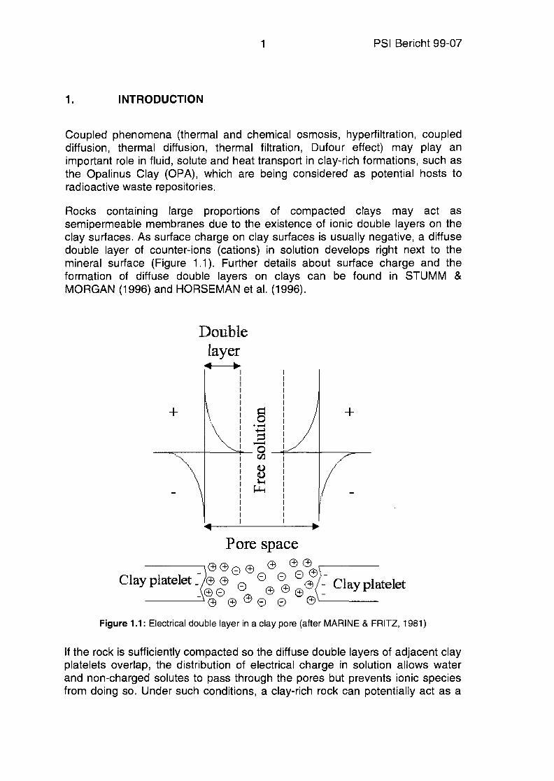
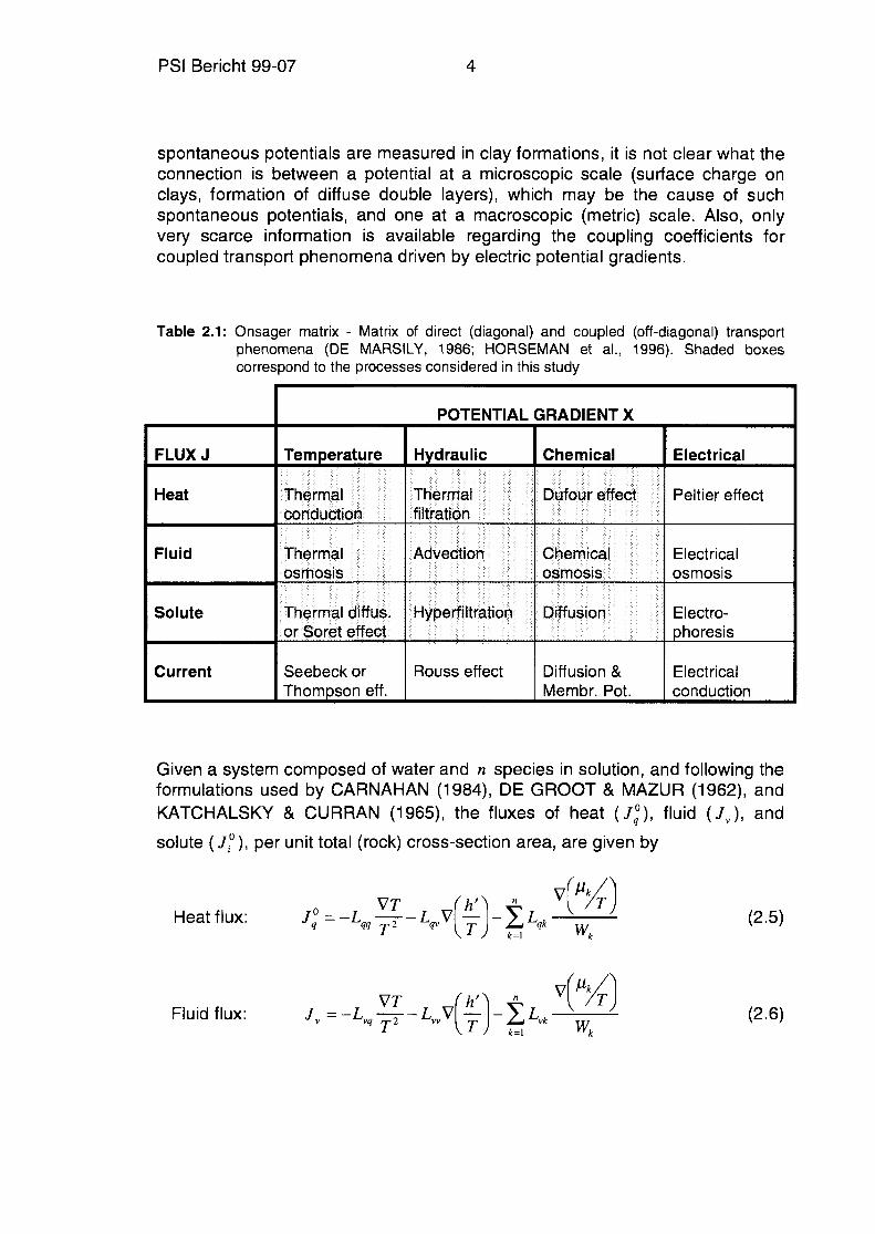

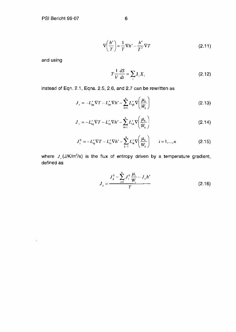
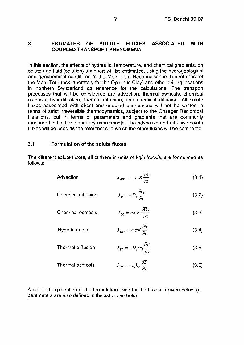

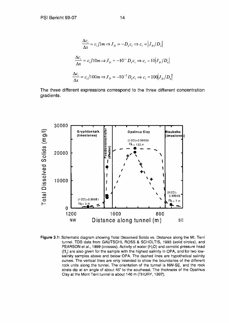


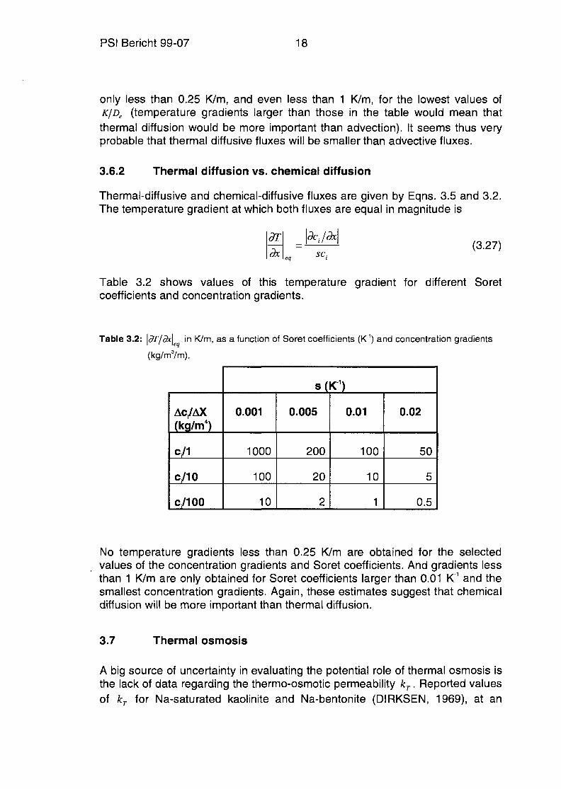

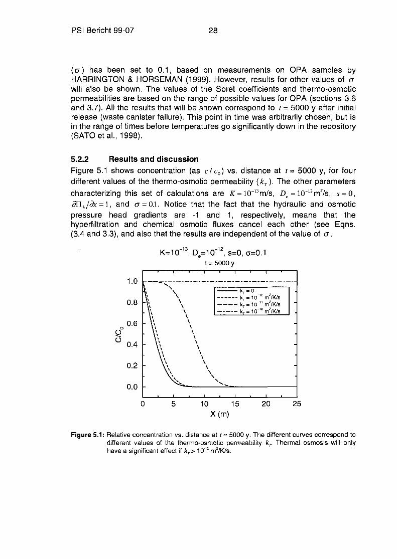


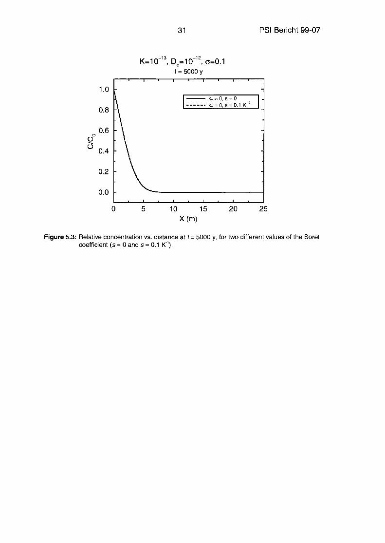
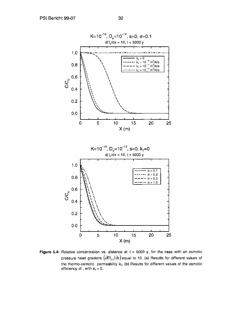
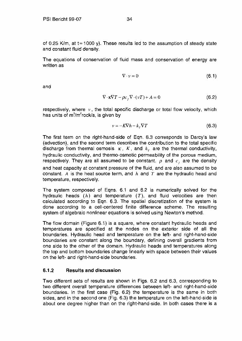
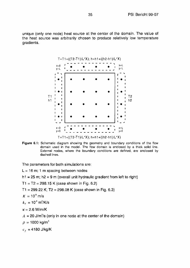
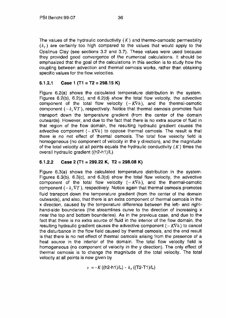
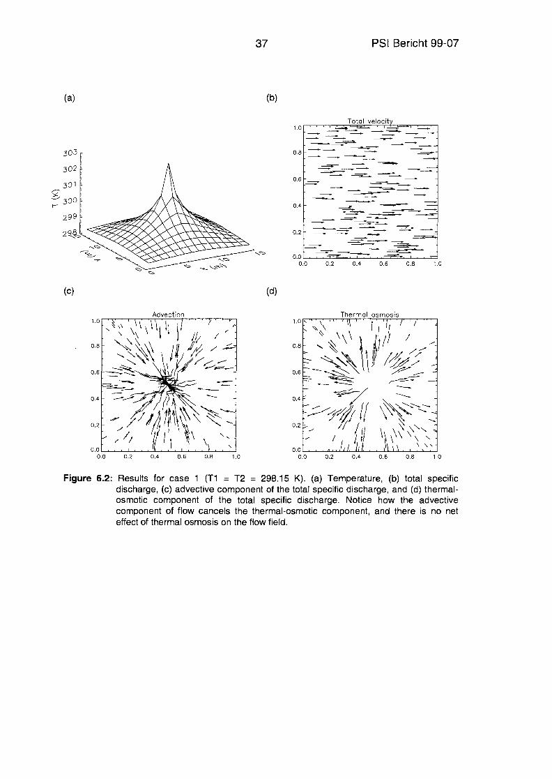
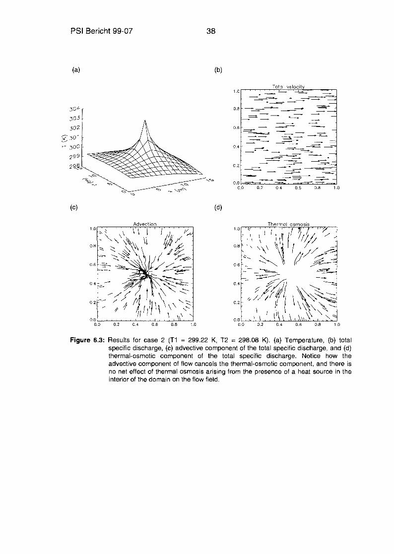
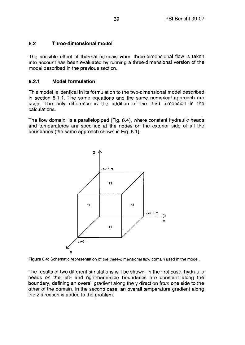
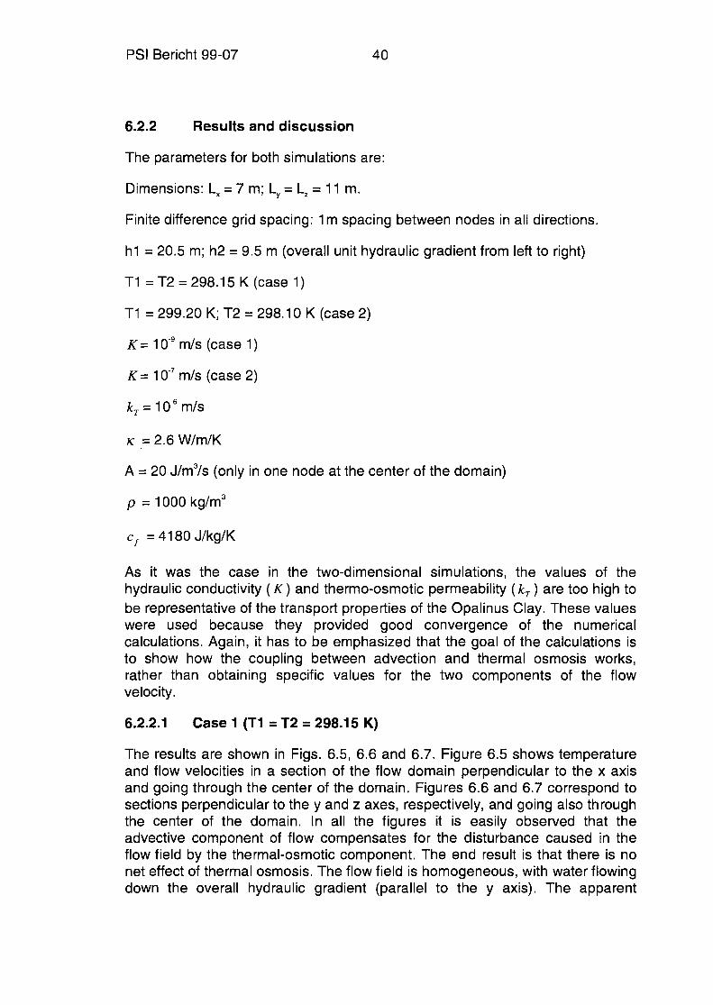
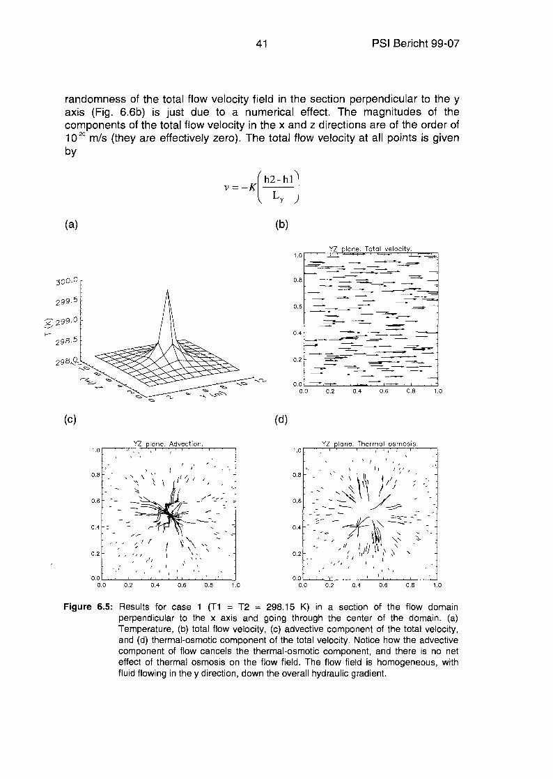
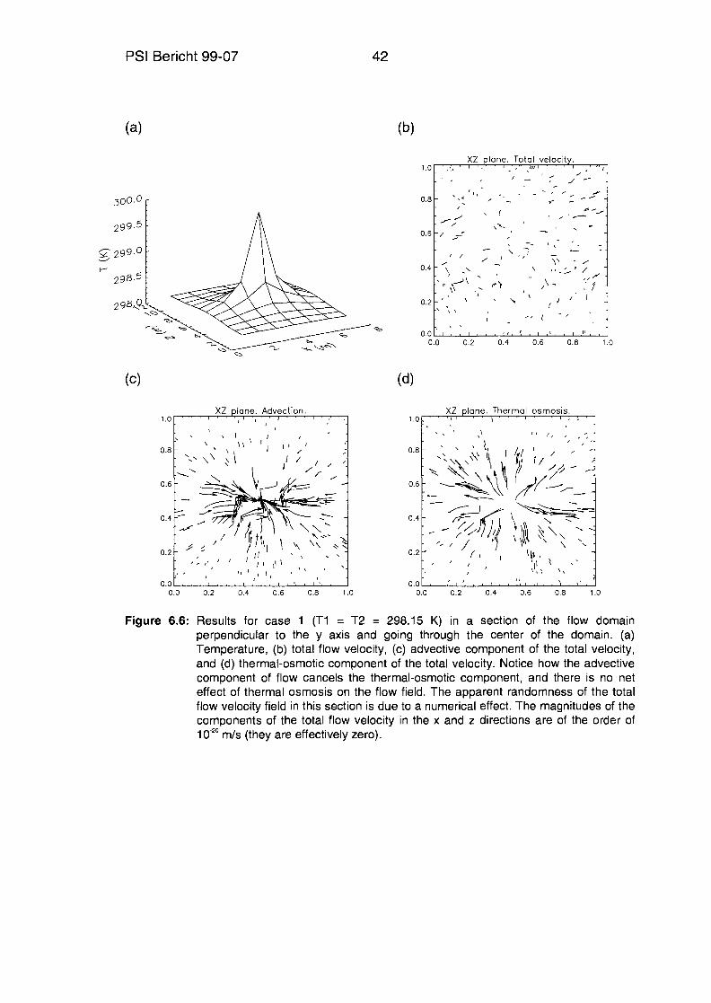
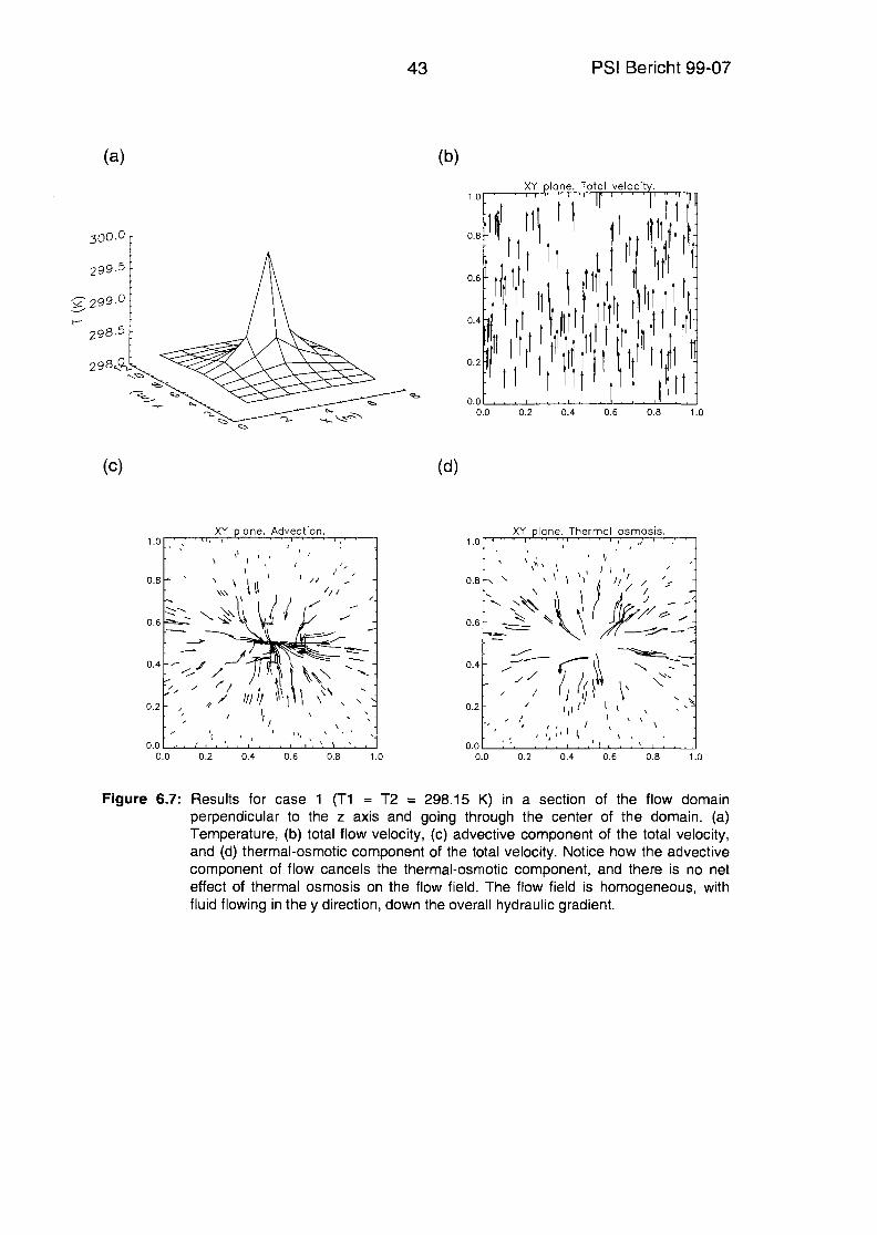
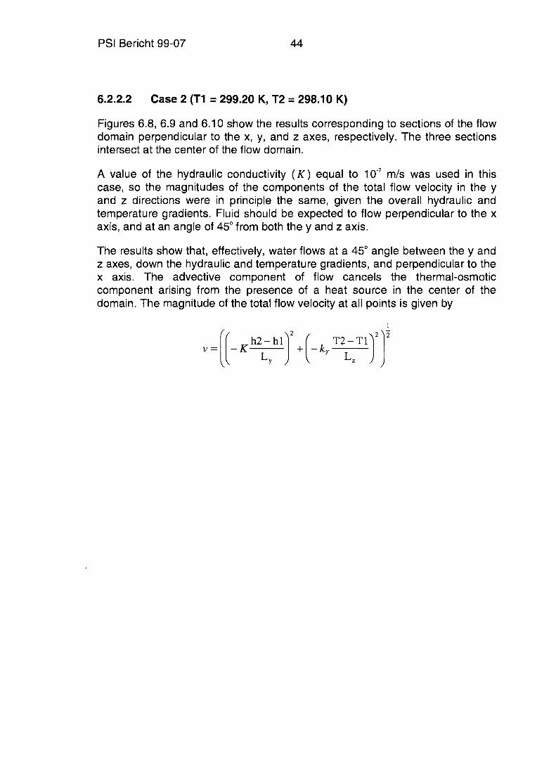
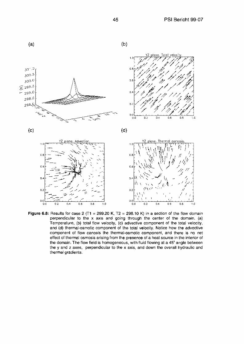
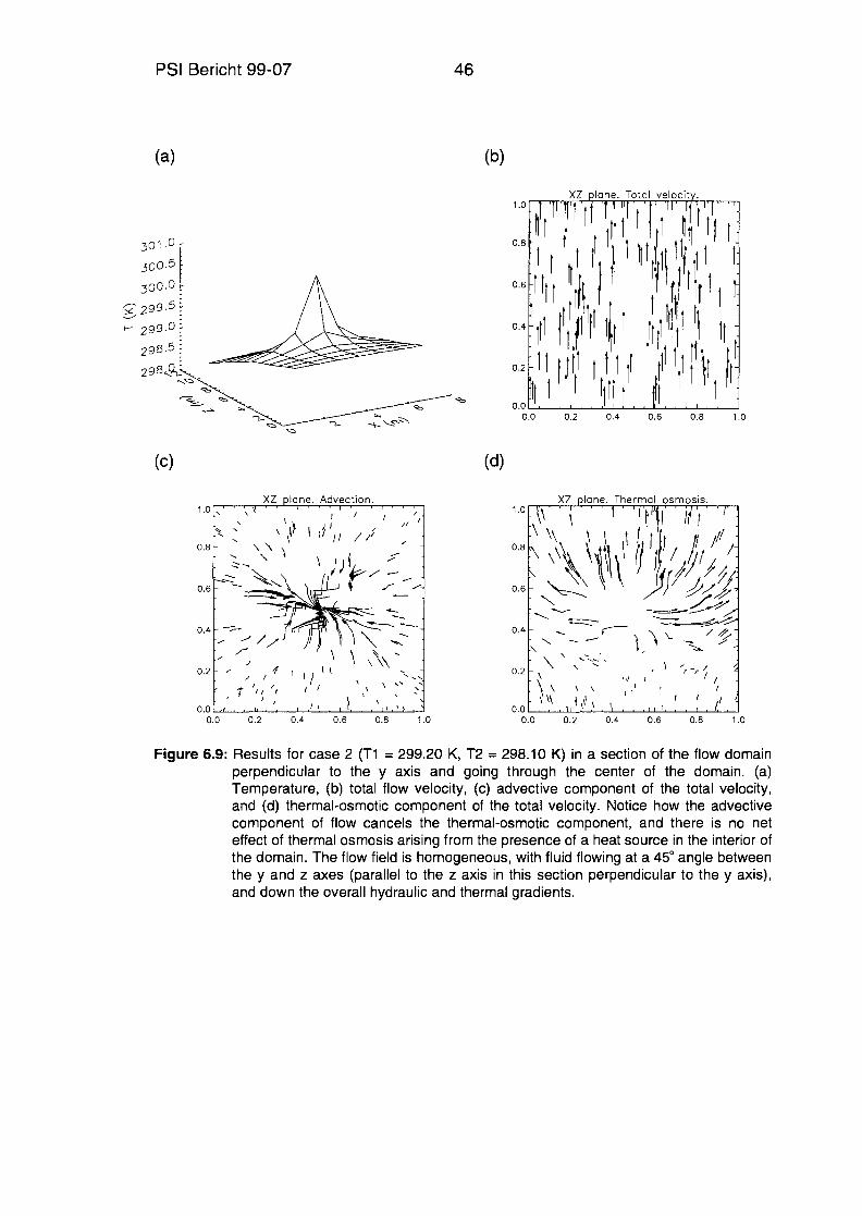
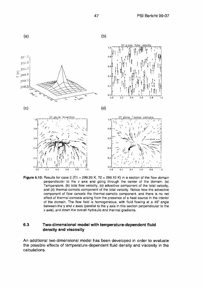
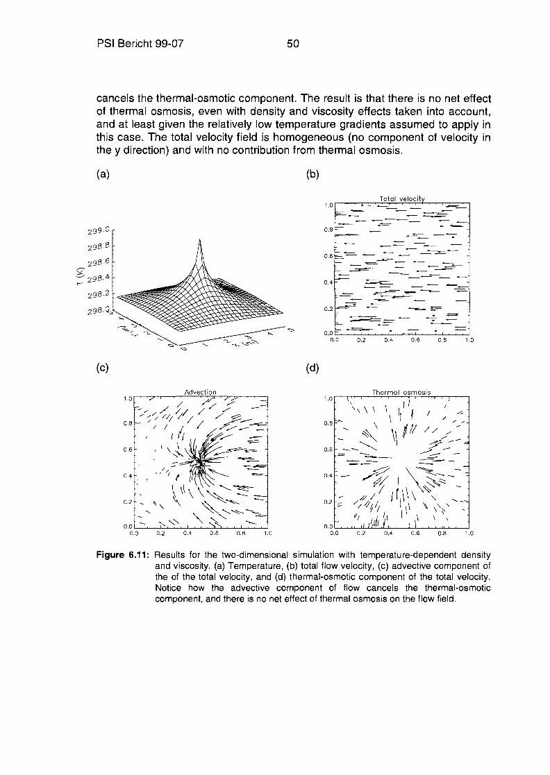
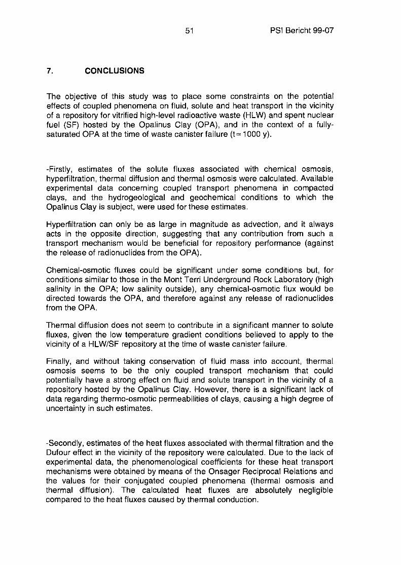
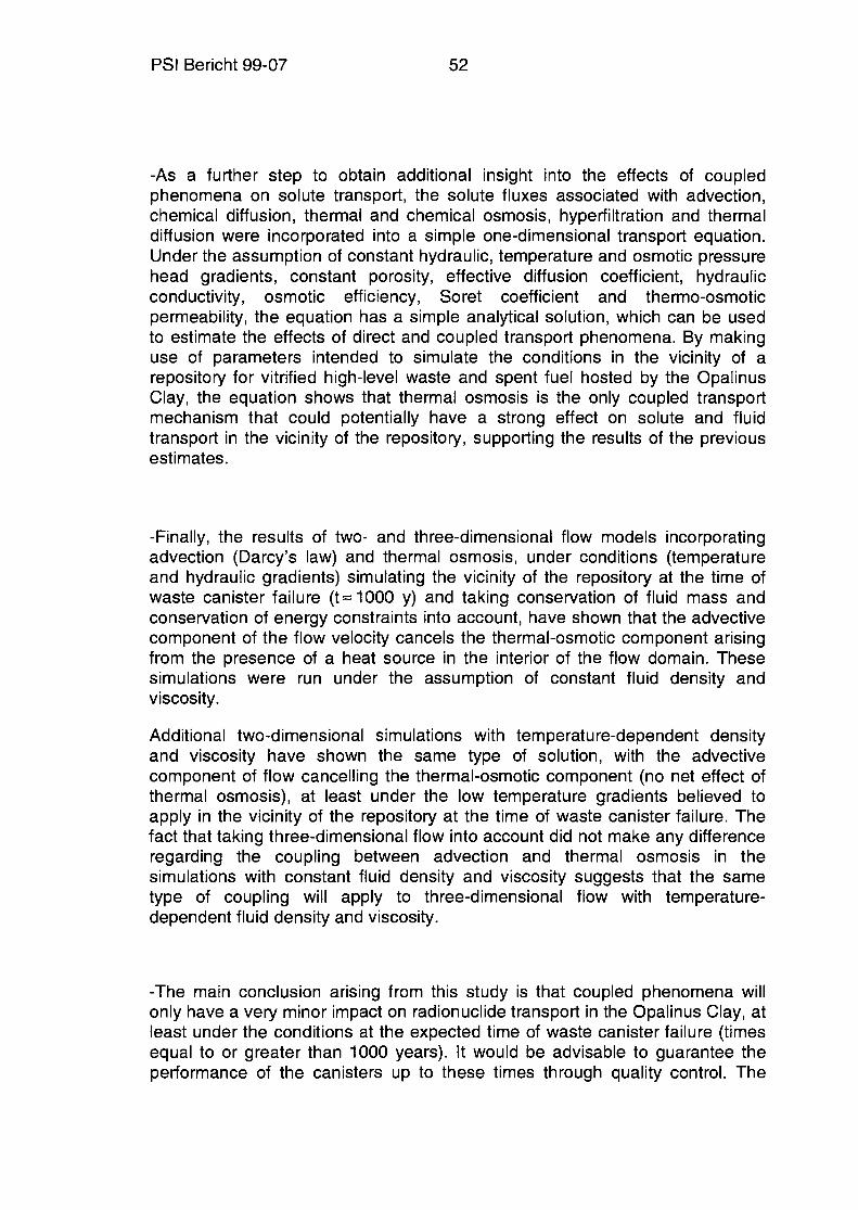


![Opalinus Clay Project - Nagra...Project Gewähr 1985 [NGB 85-01/09] – to the Federal Government at the beginning of 1985. The project demonstrated, for all waste categories, how](https://static.documents.pub/doc/80x56/5f64979385926b2ca1189789/opalinus-clay-project-nagra-project-gewhr-1985-ngb-85-0109-a-to-the.jpg)


