Couples’ and Singles’ Savings After · PDF fileWP Working Paper . 2015-322....

Working Paper WP 2015-322

Couplesrsquo and Singlesrsquo Savings After Retirement

Mariacristina De Nardi Eric French and John Bailey Jones

Project UM14-05

Couplesrsquo and Singlesrsquo Saving After Retirement

Mariacristina De Nardi University College of London Federal Reserve Bank of Chicago

Institute for Fiscal Studies and NBER

Eric French University College of London Federal Reserve Bank of Chicago

and Institute for Fiscal Studies

John Bailey Jones SUNY-Albany

July 2015

Michigan Retirement Research Center University of Michigan

PO Box 1248 Ann Arbor MI 48104

wwwmrrcisrumichedu (734) 615-0422

Acknowledgements This work was supported by a grant from the Social Security Administration through the Michigan Retirement Research Center (Grant RRC08098401) The findings and conclusions expressed are solely those of the authors and do not represent the views of the Social Security Administration any agency of the federal government or the Michigan Retirement Research Center

Regents of the University of Michigan Michael J Behm Grand Blanc Mark J Bernstein Ann Arbor Laurence B Deitch Bloomfield Hills Shauna Ryder Diggs Grosse Pointe Denise Ilitch Bingham Farms Andrea Fischer Newman Ann Arbor Andrew C Richner Grosse Pointe Park Katherine E White Ann Arbor Mark S Schlissel ex officio

Abstract

We model and compare the saving behavior of retired couples and singles These households face uncertain longevity and medical expenses in the presence of means-tested social insurance and bequest motives toward spouses and other heirs Using AHEAD data we evaluate the relative exposure of couples and singles to various risks and the relative importance of various savings motives We find that people who are single at age 70 live shorter lives than people of the same age in a couple Despite their shorter lives singles are more likely to end up in a nursing home in any given year For this reason singles have higher medical spending per person than people who are part of a couple We also find that assets drop sharply between $30000 and $60000 with the death of a spouse By the time the second spouse dies a large fraction of the wealth of the original couple has vanished with most of the declines occurring at the times of the spousesrsquo deaths A large share of these wealth drops is explained by the high medical expenses at the time of death In fact total out-of-pocket medical spending and death expenses are approximately $20000 during the year of death (whereas medical spending is $6000 per year for similarly-aged people who do not die) These facts suggest that a significant fraction of all assets held in retirement are used to self-insure against the risk of high medical and death expenses

Citation

De Nardi Mariacristina Eric French and John Bailey Jones 2015 ldquoCouples and Singlesrsquo Savings After Retirementrdquo University of Michigan Retirement Research Center (MRRC) Working Paper WP 2015-322 Ann Arbor MI httpwwwmrrcisrumichedupublicationspaperspdfwp322pdf

Authorsrsquo Acknowledgements

We thank Taylor Kelley and Jeremy McCauley for excellent research assistance and the Michigan Retirement Research Center for financial support The views expressed in this paper are those of the authors and not necessarily those of the Social Security Administration or the MRRC The views of this paper are those of the authors and not necessarily those of the Federal Reserve Bank of Chicago or the Federal Reserve System

1 Introduction

In the Assets and Health Dynamics of the Oldest Old (AHEAD) datasetabout 50 of individuals age 70 or older are in a couple while about 50are single Being in a couple during retirement allows its members to pooltheir longevity and medical expense risks but also exposes each memberto their spousersquos risks including the income loss that often accompanies aspousersquos death

Much of the previous literature including our own work only studiessingles In a previous paper (De Nardi French and Jones [20]) we showthat post-retirement medical expenses and government-provided insuranceare important to explaining the saving patterns of US single retirees at allincome levels including high permanent-income individuals who keep largeamounts of assets until very late in life These savings patterns are due to twoimportant features of out-of-pocket medical expenses First out-of-pocketmedical and nursing-home expenses can be large Second average medicalexpenditures rise very rapidly with age and permanent income Medicalexpenses that rise with age provide the elderly with a strong incentive tosave and medical expenses that rise with permanent income encourage therich to be more frugal In other work we showed that heterogeneous lifeexpectancy is important to matching the savings patterns of retired elderlysingles (De Nardi French and Jones [19])

In this paper we build on these previous contributions by studying thedeterminants of retirement saving for both couples and singles in a frame-work that incorporates observed heterogeneity in life expectancy and medicalexpenses and that explicitly models means-tested social insurance

Our first goal is to match important facts about savings medical ex-penses and longevity for both singles and couples Our second goal is toestimate couplesrsquo bequest motives toward the surviving spouse and otherheirs and compare them to the bequest motives of single people Our thirdgoal is to evaluate the extent to which medical risk affects retired couplescompared to singles and whether couples can better insure such risks dueto intra-household risk-sharing and economies of scale Our fourth goal is toevaluate the potentially different responses of the saving of couples comparedto that of singles to changes in publicly-provided health insurance

Using data from the AHEAD survey we begin by documenting assetgrowth at each age for members of different cohorts for both couples andsingles We also estimate the data generating process for shocks faced by

2

post-retirement households These first-step estimates of annuitized income mortality health transitions and medical expenses provide new evidence on how these risks compare for singles and couples Making accurate compar-isons requires that we control for the retireesrsquo permanent income which in turn requires a measure of permanent income that is invariant to age and family structure One contribution of this paper is that we construct such a measure Our approach is to estimate a model expressing annuitized income as a function of an age polynomial family structure (households are classified as couples single men or single women) family structure interacted with an age trend and a household fixed effect The fixed effect captures the notion of permanent income because it measures the component of retirement income not affected by age or changes in household structure Because annuitized retirement income is mostly from Social Security and private pensions and income from these sources is monotonically rising in lifetime income this is a good measure of permanent income (PI) Another important benefit of our methodology is that our model can be used to infer the effects of changing age or family structure on annuitized income for the same household For example our estimates imply that couples in which the male spouse dies at age 80 suffer a 40 decline in income while couples in which the female spouse dies at age 80 suffer a 30 decline These income losses are consis-tent with the fact that the spousal benefits associated with Social Security and defined benefit pensions typically replace only a fraction of the deceased spouses income

We estimate health transitions and mortality rates simultaneously byfitting the transitions observed in the HRS to a multinomial logit model We allow the transition probabilities to depend on age sex current health status marital status permanent income and interactions of these variables Using the estimated transition probabilities we simulate demographic histories beginning at age 70 for different gender-PI-health combinations We find that rich people women married people and healthy people live much longer than their poor male single and sick counterparts For example a single 70-year-old male at the 10th permanent income percentile in a nursing home expects to live only 29 more years while a single female at the 90th percentile in good health expects to live 165 more years A 70-year-old married female at the 90th percentile in good health (married to a 73 year old man in the same health state) expects to live 186 more years These large differences in life expectancy can have a significant effect on asset holdings over the retirement period (De Nardi French and Jones [19])

3

Despite having shorter lifetimes than people who are part of a couplepeople who are singles at age 70 are more likely to end up in a nursinghome than their counterparts who are members of a couple For that reasonsingles also have higher medical spending per person than people who arepart of a couple at any given age We also find that the strongest predictorfor nursing home entry is gender men are less likely to end up in a nursinghome than women Single men and women face on average a 21 and 36chance respectively of being in a nursing home for an extended stay Thecorresponding odds for married individuals are 19 and 36

We also find that assets drop sharply during the period before death Bythe time the second spouse dies a large fraction of the wealth of the originalcouple has vanished with wealth falls at the time of death of each spouseexplaining most of the decline Depending on the specification assets decline$30000-$60000 at the time of an individualrsquos death A large share of thisdrop but not all of it is explained by the high medical expenses at the time ofdeath For example out of pocket medical spending plus death expenses areapproximately $20000 during the year of death (whereas medical spendingis $6000 per year for similarly aged people who do not die)

We then estimate the preference parameters of the model with the methodof simulated moments In particular we compare the simulated asset profilesgenerated by the model to the empirical asset profiles generated by the dataand find the parameter vector that yields the closest match In matchingthe model to the data we take particular care to control for cohort effectsMoreover by explicitly modeling demographic transitions we account formortality bias

Our second-step estimates will allow us to evaluate to what extent the risksharing and economies of scale of a couple help insure against longevity andmedical-expense risk and to what extent couples get a better or worse dealfrom publicly provided health insurance They will also allow us to estimatebequest motives towards the surviving spouse in contrast to bequests tochildren or others Finally it will enable us to study in what ways theresponses of a couple will differ from the responses of a single person whenfor example public health insurance becomes more limited or its qualityworsens or some of its means-testing criteria become tighter

The rest of the paper is organized as follows In section 2 we describe thekey previous papers on which our paper builds on In section 3 we introduceour model and in section 4 we discuss our estimation procedure In section 5we describe some key features of the data and the estimated shock processes

4

that households face We discuss our results in section 6 and we and concludein section 7

2 Related Literature

Poterba et al ([43]) show that relatively little dissaving occurs amongstretirees whose family composition does not change but that assets fall signif-icantly when households lose a spouse We find similar results Furthermoreas in French et al( [26]) we document significant drops in assets when thelast member of the household passes away

Previous literature had shown that high income individuals live longerthan low income individuals (see Attanasio and Emmerson [4] and Deatonand Paxon [17]) This means that high income households must save a largershare of their lifetime wealth if they are to smooth consumption over theirretirement Differential mortality rates thus provide a potential explanationfor why high income households have higher savings rates than low incomehouseholds We extend the analysis along this dimension by explicitly mod-eling the interaction of life expectancy for individuals in couples and thedifferential life expectancy for couples and singles

Even in presence of social insurance such as Medicare and Medicaidhouseholds face potentially large out-of-pocket medical and nursing homeexpenses (see French and Jones [28 27] Palumbo [41] Feenberg and Skin-ner [25] and Marshall et al [36]) The risk of incurring such expenses mightgenerate precautionary savings over and above those accumulated againstthe risk of living a very long life ([35])

Hubbard Skinner and Zeldes [32] argue that means-tested social insur-ance programs such as Supplemental Security Income and Medicaid providestrong incentives for low income individuals not to save De Nardi et al [21]finds that these effects extend to singles in higher permanent income quin-tiles as well In this paper to allow for these important effects we modelmeans-tested social insurance explicitly for both singles and couples

Bequest motives could be another reason why households and especiallythose with high permanent income retain high levels of assets at very old ages(Dynan Skinner and Zeldes [23] and Americks et al [2]) De Nardi [15] andCastaneda et al [13] argue that bequest motives are necessary to explainwhy the observed distribution of wealth is more skewed and concentratedthan the distribution of income (Quadrini et al [18]) De Nardi et al [21]

5

shows that bequest motives help fit both assets and Medicaid recipiencyprofiles for singles We allow for a richer structure of bequest motives in thatcouples might want to leave resources to the surviving spouse children and other heirs while singles might want to leave bequests to children and otherheirs

Previous quantitative papers on savings have used simpler models thatomit one or more of these features Hurd [33] estimates a structural modelof bequest behavior in which the time of death is the only source of uncer-tainty Palumbo [41] focuses on the effect of medical expenses and uncertainlifetimes but omits bequests Dynan Skinner and Zeldes [23 24] consider the interaction of mortality risk medical expense risk and bequests but use a stylized two-period model Moreover none of these papers model householdsurvival dynamics assuming instead that households (while ldquoaliverdquo) alwayshave the same composition In contrast we explicitly model household sur-vival dynamics when the first household member dies assets are optimallysplit among the surviving spouse and other heirs Although Hurd [34] extendshis earlier model to include household survival dynamics he omits medicalexpense risk and in contrast to his earlier work he does not estimate hismodel

Our work also complements the one on retirement behaviour by couplesby Blau and Gilleskie [8] Casanova [12] and Gallipoli and Turner [30]

Including couples and simultaneously considering bequest motives socialinsurance uncertain medical expenses and uncertain life expectancy is im-portant for at least two reasons First Dynan Skinner and Zeldes [24] argue that explaining why the rich have high savings rates requires a model with precautionary motives bequest motives and social insurance Second si-multaneously considering multiple savings motives allows us to identify their relative strengths This is essential for policy analysis For example the effects of estate taxes depend critically on whether rich elderly households save mainly for precautionary reasons or mainly to leave bequests (see for example Gale and Perozek [29])

3 The Model

Consider a retired household with family structure ft (either a single per-son or a couple) seeking to maximize its expected lifetime utility at householdhead age t t = tr tr + 1 T + 1 where tr is the retirement age while T is

6

the maximum potential lifespanWe use w to denote women and h to denote men Each personrsquos health

status hsg g h wisin can vary over time The person is either in a nursinghome (hsg = 1) in bad health (hsg = 2) or in good health (hsg = 3)

For tractability we assume a fixed age gap between the husband and thewife in a couple so that one age is sufficient to characterize the householdTo be consistent with the data frequency and to reduce computation timeour time period is two years long

31 Preferences

Households maximize their utility by choosing savings bequests and cur-rent and future consumption The annual discount factor is given by β Each period the householdrsquos utility depends on its total consumption c and the health status of each member The within-period utility function for a single is given by

u(c hs) = (1 + δ(hs))c1minusν

1 νminus (1)

with ν 0ge When δ() = 0 health status does not affect utilityWe assume that the preferences of couples can be represented by the

following utility function1

uc(c hsh hsw) = [1 + δ(hsh) + 1 + δ(hsw)](cη)1minusν

1 νminus (2)

where 1 lt η 2le determines the extent to which couples enjoy economies ofscale in the transformation of consumption goods to consumption services

When a household member dies the estate can be left to the survivingspouse (if there is one) or to other heirs including the householdrsquos childrenEstates are subject to estate taxes but the exemption level during the timeperiod in our sample is above the actual assets of the vast majority of thehouseholds in our sample For this reason we abstract from explicitly mod-eling estate taxation

We indicate with b the part of the estate that does not go to the surviving spouse and assume that the deceased member of the household derives utility

1Mazzocco [37] shows that under full commitment the behavior of a couple can becharacterized by a unique utility function if the husband and wife share identical discountfactors identical beliefs and Harmonic Absolute Risk Aversion utility functions with iden-tical curvature parameters

7

θj(b) from leaving that part of the estate to heirs other than the spouse Thesubscript j indicates whether there is a surviving spouse or not and whetherone or two people have just died In particular θ0(b) gives the utility frombequests for a single person with no surviving spouse θ1(b) gives the utilityfrom bequests when there is a surviving spouse and that θ2(b) gives the utilityfrom bequests when both spouses die at the same time More specificallythe bequest function takes the form

θj(b) = φj

(b+ kj)(1minusν)

1 ν (3)

where kj determines the curvature of the bequest function and φj deter-mines its intensity Our formulation can support several interpretations of the ldquobequest motiverdquo dynastic or ldquowarm glowrdquo altruism (as in Becker and Tomes [6] or Andreoni [3]) strategic motives (as in Bernheim Schleifer and Summers [7] or Brown [9]) or some form of utility from wealth itself as in (Carroll [11] and Hurd [33])

32 Technology and Sources of Uncertainty

We assume that nonasset income at time t yt is a deterministic function of the householdrsquos permanent income I age family structure and gender if single

yt( = y(I t ft gt) (4)

There are several sources of uncertainty1) Health status uncertainty The transition probabilities for the health

status of a person depend on onersquos current health status permanent incomeage and gender and marital status Hence the elements of the health statustransition matrix for a person of gender g are given by

πgt (middot) = Pr(hsgt+1|I t g hsgt ft) (5)

2) Survival uncertainty Let sgt ( ) = s(I t g hsgt ft)middot denote the probabil-ity that an individual of gender g is alive at age t + 1 conditional on beingalive at age t having time-t health status hsg enjoying household permanentincome I and having family structure ft

3) Medical expense uncertainty at the household level We define mt asthe sum of all out-of-pocket medical expenses including insurance premiaand medical expenses covered by the consumption floor We assume that

8

medical expenses depend upon the health status of each family memberhousehold permanent income family structure gender if single age and anidiosyncratic component ψt

lnmt = m(hsht hswt I g t ft ftminus1) + σ(hsht hs

wt I g t ft ftminus1) ψt (6)

For medical spending we also include last periodrsquos household status to cap-ture the jump in medical spending that occurs in the period a family memberdies

Following Feenberg and Skinner [25] and French and Jones [27] we assumethat ψt can be decomposed as

ψt = ζt + ξt ξt N(0 σ2ξ ) (7)

ζt = ρmζtminus1 + ǫt ǫt N(0 σ2ǫ ) (8)

where ξt and ǫt are serially and mutually independent In practice wediscretize ξ and ζ using quadrature methods described in Tauchen andHussey [46]

The timing is the following at the beginning of the period the healthshock and the medical cost shocks are realized income is received and ifthe household qualifies means-tested transfers are also received Then thehousehold consumes and saves Finally the survival shock hits Householdmembers who die leave assets to their heirs Bequests are included in theheirsrsquo assets at the beginning of next period

Let us denote assets at the beginning of the period with at Assets have tosatisfy a borrowing constraint at 0ge Let us indicate the constant and risk-free rate of return with r and total post-tax income with y(r at + yt( ) τ)middotwith the vector τ describing the tax structure

33 Recursive Formulation

To save on state variables we follow Deaton [16] and redefine the problemin terms of cash-on-hand

xt = at + y(r at + yt( ) τ) mt + trt( )middot minus middot (9)

The law of motion for cash on hand next period is given by

xt+1 = xt minus ct minus bt + y r (xt minus ct) + yt+1(middot) τ minusmt+1 + trt(middot) (10)

9

where bt 0ge is positive only when one spouse from a couple dies during thecurrent period and leaves bequests to other heirs (eg children) We do notinclude received bequests as a source of income because very few householdsaged 65 or older receive them When all household members die their assetsare bequeathed to the remaining heirs

Following Hubbard et al [31 32] we assume that the government pro-vides means-tested transfers trt(middot) that bridge the gap between a minimumconsumption floor and the householdrsquos resources net of an asset disregardamount Define the resources available next period before government trans-fers with

xt+1 = xt minus ct minus bt + y r (xt minus ct) + yt+1(middot) τ minusmt+1( )

(11)

Consistently with the main Medicaid and SSI rules we can express govern-ment transfers next period as

trt+1(xt+1 hst+1) = max 0 cmin(ft+1) max 0 xt+1 ad(ft+1) (12)

We allow both the guaranteed consumption level cmin and the asset disregardad to vary with family structure We impose that if transfers are positivect = cmin(ft)

The law of motion for cash on hand next period can thus be rewritten as

xt+1 = xt+1 + trt+1(xt+1 hst+1) (13)

To ensure that cash on hand is always non-negative we require

ct le xt forallt (14)

Using the definition of cash-on-hand the value function for a single indi-vidual of gender g can be written as

V gt (xt hst I ζt) = max

ctxt+1

u(ct hst) + βs(I t g hsgt ft)Et V gt+1(xt+1 hst+1 I ζt+1)

+ β(1minus s(I t g hsgt ft)θ0(xt minus ct)

( )

(15)

subject to equations (4)-(8) and(11)-(14)

minus minus

10

The value function for couples can be written as

uc

V ct (xt hs

ht hs

wt I ζt) = max

ctxt+1bwbh(ct hs

ht hs

wt )

+ βs(I t w hsgt 1)s(I t h hsgt 1)Et

(V ct+1(xt+1 hs

ht+1 hs

wt+1 I ζt+1)

)

+ βs(I t w hsgt 1)(1minus s(I t h hsgt 1))[Et

(V wt+1(x

wt+1 hs

wt+1 I ζt+1)

)+ θ1(b

ht )]

+ β(1minus s(I t w hsgt 1))s(I t h hsgt 1)

[Et

(V ht+1(x

ht+1 hs

ht+1 I ζt+1)

)+ θ1(b

wt )]+

β(1minus s(I t w hsgt 1)(1minus s(I t h hsgt 1)θ2(xt minus ct)

(16)

where the value function is subject to equations subject to equations (4)-(8)and (11)-(17) with ft = 1 since we are referring to couples and bequests areconstrained by

bt le xt minus ct (17)

4 Estimation Procedure

We adopt a two-step strategy to estimate the model In the first stepwe estimate or calibrate those parameters that given our assumptions canbe cleanly identified outside our model In particular we estimate healthtransitions out-of-pocket medical expenses and mortality rates from rawdemographic data We calibrate the household economies of scale parameterand the minimum consumption floor for singles and couples based on previouswork

In the second step we estimate the rest of the modelrsquos parameters (dis-count factor risk aversion health preference shifter and bequest parameters)

∆ = (β ν δ ω φ0 φ1 φ2 k0 k1 k2)

with the method of simulated moments (MSM) taking as given the param-eters that were estimated in the first step In particular we find the param-eter values that allow simulated life-cycle decision profiles to ldquobest matchrdquo(as measured by a GMM criterion function) the profiles from the data

Because our underlying motivations are to explain why elderly individualsretain so many assets and to explain why individuals with high income save

11

at a higher rate we match median assets by cohort age and permanent income Because we wish to study differences in savings patterns of couples and singles we match profiles for the singles and couples separately Finally to help identify bequest motives toward ones spouse we also match the fraction of assets (net worth) left to the surviving spouse in a couple affected by death

In particular the moment conditions that comprise our estimator aregiven by

12

1 Median asset holdings by PI-cohort-year for the singles who are stillalive when observed

2 Median asset holdings by PI-cohort-year for those who were initiallycouples with both members currently alive

When there is a death in a couple the surviving spouse is includedin the singlesrsquo profile of the appropriate age cohort and permanentincome cell in keeping with our assumption that all singles differ onlyin their state variables

3 For estates of positive value the median fraction of the estate left to thesurviving spouse by PI and age We do not condition this moment bycohort for two reasons First the sample size is too small and secondthere does not seem to be a discernible cohort effect in this moment

The cells are computed as follows2 Household i has family structure ftwhich indexes households that are initially couples and those that either areinitially singles (both men and women) or become singles through deathof their spouse We sort type-f households in cohort c by their permanentincome levels separating them into Q = 5 quintiles Suppose that householdirsquos permanent income level falls in the qth permanent income interval ofhouseholds in its cohort and family structure

Let acfqt(∆ χ) be the model-predicted median observed asset level incalendar year t for a household that was in the qth permanent income intervalof cohort c Assuming that observed assets have a continuous density at theldquotruerdquo parameter vector (∆0 χ0) exactly half of the households in group

2As was done when constructing the figures from the HRS data we drop cells with lessthan 10 observations from the moment conditions Simulated agents are endowed withasset levels drawn from the 1996 data distribution and thus we only match asset data1998-2010

cfqt will have asset levels of acfqt(∆0 χ0) or less This leads to the followingmoment condition

( )E 1ait acfqt(∆0 χ0) 12 |c f q t household alive at t = 0 (18)

for all c f q and t In other words for each permanent income-familystructure-cohort grouping the model and the data have the same medianasset levels

The mechanics of our MSM approach are as follows We compute life-cycle histories for a large number of artificial households Each of thesehouseholds is endowed with a value of the state vector (t ft xt I hs

ht hs

wt ζt)

drawn from the data distribution for 1996 and each is assigned the entirehealth and mortality history realized by the household in the AHEAD datawith the same initial conditions This way we generate attrition in our simu-lations that mimics precisely the attrition relationships in the data (includingthe relationship between initial wealth and mortality)

We discretize the asset grid and using value function iteration we solvethe model numerically This yields a set of decision rules which in combina-tion with the simulated endowments and shocks allows us to simulate eachindividualrsquos assets medical expenditures health and mortality We computeassets from the artificial histories in the same way as we compute them fromthe real data We use these profiles to construct moment conditions andevaluate the match using our GMM criterion We search over the parame-ter space for the values that minimize the criterion Appendix E contains adetailed description of our moment conditions the weighting matrix in ourGMM criterion function and the asymptotic distribution of our parameterestimates

When estimating the life-cycle profiles and subsequently fitting the modelto those profiles we face two well-known problems First in a cross-sectionolder households were born in an earlier year than younger households andthus have different lifetime incomes Because lifetime incomes of householdsin older cohorts will likely be lower than the lifetime incomes of youngercohorts the asset levels of households in older cohorts will likely be loweralso Therefore comparing older households born in earlier years to youngerhouseholds in later years leads to understate asset growth Second house-holds with lower income and wealth tend to die at younger ages than richerhouseholds Therefore the average survivor in a cohort has higher lifetimeincome than the average deceased member of the cohort As a result ldquomor-tality biasrdquo leads the econometrician to overstate the average lifetime income

13

of members of a cohort This bias is more severe at older ages when a greatershare of the cohort members are dead Therefore ldquomortality biasrdquo leads tooverstate asset growth

We use panel data to overcome these first two problems Because we aretracking the same households over time we are obviously tracking membersof the same cohort over time Similarly we do separate sets of simulationsfor each cohort so that the (initial) wealth and income endowments behindthe simulated profiles are consistent with the endowments behind the empir-ical profiles As for the second problem we explicitly simulate demographictransitions so that the simulated profiles incorporate mortality effects in thesame way as the data both for couples and singles

5 Data

We use data from the Asset and Health Dynamics Among the Oldest Old (AHEAD) dataset The AHEAD is a sample of non-institutionalized individuals age 70 or older in 1993 These individuals were interviewed in late 1993early 1994 and again in 1996 1998 2000 2002 2004 2006 2008 and 2010 We do not use 1994 assets nor medical expenses due to underreporting (Rohwedder et al [45])

We only consider retired households to abstract from the retirement de-cisions and focus on the determinants of savings and consumption Becausewe only allow for household composition changes through death we drophouseholds where an individual enters a household or an individual leavesthe household for reasons other than death Fortunately attrition for rea-sons other than death is a minor concern in our data

To keep the dynamic programming problem manageable we assume afixed difference in age between spouses and we take the average age differencefrom our data In our sample husbands are on average 3 years older thantheir wives To keep the data consistent with this assumption we drop allhouseholds where the wife is more than 4 years older or 10 years youngerthan her husband

We begin with 6047 households After dropping 401 households who get married divorced were same sex couples or who report making other transitions not consistent with the model 753 households who report earning at least $3000 in any period 171 households with a large difference in the age of husband and wife and 87 households with no information on the spouse

14

in a household we are left with 4634 households of whom 1388 are couplesand 3246 are singles This represents 24274 household-year observationswhere at least one household member was alive

We break the data into 5 cohorts The first cohort consists of individualsthat were ages 72-76 in 1996 the second cohort contains ages 77-81 thethird ages 82-86 the fourth ages 87-91 and the final cohort for samplesize reasons contains ages 92-102 Even with the longer age interval thefinal cohort contains relatively few observations In the interest of claritywe exclude this cohort from our graphs but we use all cells with at least 10observations when estimating the model

We use data for 8 different years 1996 1998 2000 2002 2004 2006 2008and 2010 We calculate summary statistics (eg medians) cohort-by-cohortfor surviving individuals in each calendar yearmdashwe use an unbalanced panelWe then construct life-cycle profiles by ordering the summary statistics bycohort and age at each year of observation Moving from the left-hand-sideto the right-hand-side of our graphs we thus show data for four cohorts witheach cohortrsquos data starting out at the cohortrsquos average age in 1996

Since we want to understand the role of income we further stratify thedata by post-retirement permanent income (PI) Hence for each cohort ourgraphs usually display several horizontal lines showing for example medianassets in each PI group in each calendar year These lines also identify themoment conditions we use when estimating the model

Our PI measure can be thought of as the level of income if there were two people in the household at age 70 We measure post-retirement PI using non-asset nonsocial insurance annuitized income and the methods described in appendix A The method maps the relationship between current income and PI adjusted for age and household structure The income measure includes the value of Social Security benefits defined benefit pension benefits veterans benefits and annuities Since we model means-tested social insurance from SSI and Medicaid explicitly through our consumption floor we do not include SSI transfers Because there is a roughly monotonic relationship between lifetime earnings and the income variables we use our measure of post-retirement PI is also a good measure of lifetime permanent income

The AHEAD has information on the value of housing and real estateautos liquid assets (which include money market accounts savings accounts T-bills etc) IRAs Keoghs stocks the value of a farm or business mutual funds bonds ldquootherrdquo assets and investment trusts less mortgages and other debts

15

We do not include pension and Social Security wealth for four reasonsFirst we wish to to maintain comparability with other studies (Hurd [33]Attanasio and Hoynes [5] for example) Second because it is illegal to borrowagainst Social security wealth pension and difficult to borrow against mostforms of pension wealth Social Security and pension wealth are much moreilliquid than other assets Third their tax treatment is different from otherassets Finally differences in Social Security and pension are captured inour model by differences in the permanent income measure we use to predictannual income

One important problem with our asset data is that the wealthy tendto underreport their wealth in virtually all household surveys (Davies andShorrocks [14]) This will lead us to understate asset levels at all ages How-ever Juster et al (1999) show that the wealth distribution of the AHEADmatches up well with aggregate values for all but the richest 1 of house-holds Given that we match medians (conditional on permanent income)underreporting at the very top of the wealth distribution should not seri-ously affect our results

6 Results

61 Health and Mortality

We estimate health transitions and mortality rates simultaneously byfitting the transitions observed in the HRS to a multinomial logit model Weallow the transition probabilities to depend on age sex current health statusmarital status permanent income as well as polynomials and interactions ofthese variables

Using the estimated transition probabilities we simulate demographichistories beginning at age 70 for different gender-PI-health combinationsTables 1 and 2 show life expectancies for singles and couples at age 70respectively All tables use the appropriate distribution of people over statevariables to compute the number which is object of interest We find thatrich people women married people and healthy people live much longerthan their poor male single and sick counterparts

Table 1 shows that a single male at the 10th permanent income percentilein a nursing home expects to live only 29 more years while a single femaleat the 90th percentile in good health expects to live 165 more years The

16

far right column shows average life expectancy conditional on permanent income averaging over both genders and all health states It shows that singles at the 10th percentile of the permanent income distribution live on average 115 years whereas singles at the 90th percentile live on average 147 years

Table 1 Life expectancy in years for singles conditional on reaching age 70

Males FemalesNursingHome

BadHealth

GoodHealth

NursingHome

BadHealth

GoodHealth All

IncomePercentile

10 286 672 845 379 1113 1321 114630 286 730 936 378 1178 1403 122050 286 799 1034 378 1248 1489 130170 288 883 1137 378 1333 1576 138590 290 976 1244 385 1414 1654 1473

By genderMen 997Women 1372

By health statusBad Health 1111Good Health 1420

Table 2 shows that a 70 year old male married to a 67 year old womanwith the same health as himself at the 10th permanent income percentile in anursing home expects to live only 27 more years while a 70 year old marriedfemale at the 90th percentile in good health (married to a 73 year old man inthe same health state as herself) expects to live 186 more years Averagingover both genders and all health states married 70 year old people at the10th percentile of the income distribution live on average 105 years whilethose at the 90th percentile live 157 years Singles at the 10th percentilelive longer than members of couples at the same percentile The reason

17

for this is that singles at the 10th percentile of the income distribution areare overwhelmingly women who live longer whereas 50 of the members ofcouples are male Conditional on gender those in either good or bad healthat the 10th percentile live longer if in a couple Conditional only on gendermembers of couples live almost 3 years longer than singles single 70 yearold women live on average 138 years versus 169 for married women But acomparison of tables 1 and 2 reveals that conditional on PI and healththe differences in longevity are much smaller Married people live longerthan singles but much of the difference is explained by the fact that marriedpeople tend to have higher PI

Table 2 Life expectancy in years for couples conditional on reaching age 70

BadHealth

GoodHealth

NursingHome

BadHealth

GoodHealth All

IncomePercentile

10 265 688 846 359 1147 1349 104830 269 777 974 367 1246 1468 115950 276 887 1112 376 1355 1598 128670 285 1019 1262 390 1489 1729 142390 298 1169 1422 406 1626 1855 1567

Oldest Survivor 1878Prob Oldest Survivor is Woman 675

18

Table 3 Probability of ever entering a nursing home singles alive at age 70

Males FemalesBad

HealthGoodHealth

BadHealth

GoodHealth All

IncomePercentile

10 208 215 340 356 32230 205 216 341 361 32750 203 217 341 368 32870 201 216 341 369 33190 195 215 339 369 330

The bottom part of table 2 shows the number of years of remaining lifeof the oldest survivor in a household when the man is 70 and the woman is67 On overage the last survivor lives and additional 188 years The womanis the oldest survivor 68 of the time

The strongest predictor for nursing home entry is gender men are lesslikely to end up in a nursing home than women Although married peopletend to live longer than singles they are slightly less likely to end up in anursing home

Table 3 shows that single men and women face on average a 21 and36 chance of being in a nursing home for an extended stay respectivelyTable 4 shows that married men and women face on average a 19 and 36chance of being in a nursing home for an extended stay Married people aremuch less likely to transition into a nursing home at any age but married

19

people often become single as their partner dies and a they age Furthermoremarried people tend to live longer than singles so they have more years oflife to potentially enter a nursing home Permanent income has only a smalleffect on ever being in a nursing home Those with a high permanent incomeare less likely to be in a nursing home at each age but they tend to livelonger

Table 4 Probability of ever entering a nursing home married alive at age70

Males FemalesBad

HealthGoodHealth

BadHealth

GoodHealth All

IncomePercentile

10 161 166 318 330 24630 166 175 323 343 25750 173 186 330 357 26570 178 194 340 364 27590 185 206 349 373 283

62 Income

We model income as a function of a third order polynomial in age dum-mies for family structure family structure interacted with an age trend anda fifth order polynomial in permanent income The estimates use a fixedeffects estimation procedures where the fixed effect is a transformation of

20

initial permanent income Hence the regression results can be interpreted asthe effect of changing age or family structure for the same household seeappendix A for details of the procedure

010

000

2000

030

000

70 80 90 100age

20th percentile couple 80th percentile couple20th percentile to female 80th percentile to female20th percentile to male 80th percentile to male

2005

dol

lars

Income by Permanent Income Percentile Initially Couples

Figure 1 Income conditional on permanent income and family structureFigure assumes all households begin as couples then potentially change to asingle male or single female at age 80

Figure 1 presents predicted income profiles for those at the 20th and80th percentiles of the permanent income distribution For each permanentincome level we display three scenarios all commencing from the income ofa couple Under the first scenario the household remains a couple until age100 Under the second one the man dies at age 80 Under the third one thewoman dies at age 80

Figure 1 shows that average annual income ranges from about $14000per year for couples in the 20th percentile of the PI distribution to over$30000 for couples in the 80th percentile of the PI distribution As a pointof comparison median wealth holdings for the two groups are $70000 and$330000 at age 74 respectively Our estimates suggest that couples in whichthe male spouse dies at age 80 suffer a 40 decline in income while couplesin which the female spouse dies at 80 suffer a 30 decline in income

21

22

These income losses at the death of a spouse reflect the fact that although both Social Security and defined benefit pensions have spousal benefits these benefits replace only a fraction of the deceased spousersquos income More specif-ically people can receive benefits either based on their own history of Social Security contributions (in which case they are a ldquoretired workerrdquo) or based on their spousersquos or former spousersquos history (in which case they receive the ldquospousersquosrdquo or ldquowidowsrdquo benefit)

A married person who never worked or who earned less than thcir spouse can receive 50 of their spousersquos benefit if their spouse is alive and is a ldquoretired workerrdquo The same person can receive up to 100 of their spousersquos benefit if their ldquoretired workerrdquo spouse has died Thus the household benefit can receive 100+50=150of the former worker spousersquos benefit when alive and 100 of the former worker spousersquos benefit when either spouse has died Thus after the death of a household member the household would maintain (100150)=67of the original Social Security benefit and would experience a 33 drop in benefits

3See httpssocialsecuritygovplannersretireyourspousehtml for more details of cal-culation of spousal benefits

In contrast a person who earned the same amount as their spouse willnot receive a spousal or widowrsquos benefit In this case both spouses in thecouple will receive 100 of their own ldquoretired workerrdquo benefit which is basedoff of their own earnings history After the death of a spouse the householdbenefit will be (100(100+100)= 50 of its level when both were alive

To perform our calculations we make several assumptions including thatboth spouses begin receiving benefits at the normal retirement age In prac-tice there are many modifications to this rule including those to account forthe age at which the beneficiary and spouse begin drawing benefits3 Our re-gression estimates capture the average drop in income at the time of death ofa spouse averaging over those who retire at different ages and have differentclaiming histories

63 Medical Spending

One drawback of the AHEAD data is that it contains information onlyon out of pocket medical spending and not on the portion of medical spend-ing covered by Medicaid To be consistent with the model in which theconsumption floor is explicitly modeled we need to include both Medicaid

payments and out of pocket medical spending in our measure of out-of-pocketmedical spending

Fortunately the Medicare Current Beneficiary Survey (MCBS) has ex-tremely high quality information on Medicaid payments and out of pocket medical spending It uses a mixture of both administrative and survey data One drawback of the MCBS however is that although it has information on marital status and household income but it does not have information on the medical spending or health of the spouse To exploit the best of both datasets we use the procedures described in Appendix C to obtain our measured out-of-pocket medical expenditures including those paid for by Medicaid

We model the logarithm of medical spending as a fourth order polynomialin age dummies for family structure the health of each family member(including whether that family member just died) family structure interactedwith an age trend and a fifth order polynomial in permanent income Aswith the income estimate we use fixed effects estimation procedures so theregression results can be interpreted as the effect of changing age or familystructure for the same household

a

010

000

2000

0

70 80 90 100age

20th percentile couple 20th percentile to female20th percentile to male

2005

dol

lars

Medical Expenses 20th Percentile of Permanent Income Initially Couples

b

010

000

2000

0

70 80 90 100age

2005

dol

lars

Figure 2 Mean out-of-pocket medical expenditures by age conditional onpermanent income and family structure Figure assumes all households beginas couples then potentially change to a single male or single female at age80

Figure 2 displays our predicted medical expense profiles for those at the20th (left panel) and 80th (right panel) percentiles of the permanent incomedistribution for those in bad health For each permanent income level we

23

present three scenarios all of which start out with a couple Under the firstscenario the household remains a couple until age 100 Under the secondone the man dies at age 80 Under the third one the woman dies at age80 The jump in medical spending shown at age 80 represents the elevatedmedical spending during the year of death of a family member and amountsto almost $5000 on average Both average medical spending and the jumpat time of death are larger for those with higher permanent income

The figure shows that before age 80 average annual medical spendinghoover around $4000 per year for the couples in both income groups Forthose at the 20th percentile of the PI distribution medical expenses changelittle with age However for couples in the 80th percentile medical expensesrise to well over $10000 per year by age 95

In order to estimate the variability of medical spending we take medi-cal expense residuals (the difference between actual and predicted medicalspending) and we regress the squared residuals on the same covariates weused for the regression for the logarithm of medical spending

64 Life-Cycle Asset Profiles

The following figures display median assets conditional on birth cohort and income quintile for couples and singles that are classified by permanent income quintile based on the permanent incomes of that same subpopulation (couples or singles) We choose to classify profiles in this fashion because cou-ples are richer than singles and classifying a subpopulation according to the permanent income of the entire population would create cells that in some cases contain a large fraction of the population while in others they generate a much smaller cell The graphs based on the classification of permanent income by the whole population are in appendix B and display similar pat-terns

Figure 3 displays the asset profiles for the unbalanced panel of singlesclassified according to the PI of the singles Median assets are increasingin permanent income with the 74-year-olds in the highest PI income of thesingles holding about $200000 in median assets while those at the lowest PIquintiles holding essentially no assets Over time those with the highest PItend to hold onto significant wealth well into their nineties those with thelower PIs never save much while those in the middle PIs display quite someasset decumulation as they age

Figure 4 reports median assets for the population of those who are ini-

24

tially in a couple The first thing to notice is that couples are richer thansingles The younger couples in the highest PI quintile for couples hold over$340000 compared to $200000 for singles and even the couples in the low-est PI quintile bin hold over $60000 in the earlier years of their retirementcompared to zero for the singles As for the singles the couples in the highestPI quintile hold on to large amount of assets well into their nineties whilethose in the lowest income PIs display more asset decumulation Some ofthese couples lose one spouse during the period in which we observe themin which case we report the assets of the surviving spouse hence some of thedecumulation that we observe in this graph is due to the death of one spouseand consequent disappearance of some of the couplersquos assets

Figure 3 Median assets for singles PI percentiles computed using singlesonly Each line represents median assets for a cohort-income cell traced overthe time period 1996-2010 Thicker lines refer to higher permanent incomegroups Solid lines cohorts ages 72-76 and 82-86 in 1996 Dashed lines ages82-86 and 92-96 in 1996

Figure 5 displays median assets for those who initially are in couples

25

and remain in a couple during our sample period That is they do notexperience the death of a partner Interestingly these graphs display flat toincreasing asset profiles going from low to high permanent income This isconsistent with the observation that much of the asset decumulation for acouple happens at death of one spouse

Figure 4 Median assets for initially couples PI percentiles computed usingcouples only Each line represents median assets for a cohort-income celltraced over the time period 1996-2010 Thicker lines refer to higher per-manent income groups Solid lines cohorts ages 72-76 and 82-86 in 1996Dashed lines ages 82-86 and 92-96 in 1996

To formalize and quantify this observation we perform regression anal-ysis We regress assets on a household fixed effect dummies for householdstatus (couple single man single woman everyone dead) a polynomial inage and interactions between these and permanent income Including thehousehold specific fixed effect means that we can track wealth of the samehouseholds when one member of the household dies The fixed effect in-cludes all time invariant factors including permanent income so we cannot

26

include permanent income directly To include permanent income directlywe then regress the estimated fixed effect on the permanent income of thathousehold

Figure 5 Median assets for intact couples PI percentiles computed usingcouples only Each line represents median assets for a cohort-income celltraced over the time period 1996-2010 Thicker lines refer to higher per-manent income groups Solid lines cohorts ages 72-76 and 82-86 in 1996Dashed lines ages 82-86 and 92-96 in 1996

Figure 6 reports the predicted assets of a couple starting out respectivelyin the top PI income quintile and in the bottom one and display the assetsunder three scenarios Under the first one the couple remains intact untilage 90 Under the second one the male dies at age 80 while under thethird one the female dies at age 80 For both PI levels assets stay roughlyconstant if both partners are alive In contrast assets display a significantdrop at death of one of the spouses for the higher PI couples The resultsshow that on average wealth declines approximately $60000 at the time ofdeath of a household member Interestingly assets experience a large drop

27

when the male dies also for the lowest PI quintile but not much of a dropwhen the female dies first

010

0000

2000

0030

0000

4000

00

70 80 90 100age

2005

dol

lars

Assets by Permanent Income Percentile Initially Couples

Figure 6 Assets conditional on permanent income and family structureFigure assumes all households begin as couples then potentially change to asingle male or single female at age 80 then everyone dies at age 90

A simpler exercise of merely tabulating the wealth decline when one mem-ber of the household dies suggests smaller estimates of the wealth decline atthe time of death of a spouse This procedure suggests a decline of wealthof $30000 at the death of a spouse A large share of this drop but not allof it is explained by the high medical expenses at the time of death Forexample out of pocket medical spending plus death expenses are approxi-mately $20000 during the year of death (whereas medical spending is $6000per year for similarly aged people who do not die)

To measure the decline in wealth at the time of death of the final memberof the family we exploit the exit surveys which include information on theheirsrsquo reports of the value of the estate In addition we also use data frompost-exit interviews which are follow up surveys of heirs to better measurewealth held in the estate The results suggest even larger declines in wealthwhen the final member of the household dies For those at the top of theincome distribution the death of a single person results in a wealth decline

28

of approximately $110000 whereas the decline is closer to $70000 for thoseat the bottom of the income distribution

One should take the wealth increase when both members of the householddie for those at the top of the income distribution with some caution sincevery few households have both members die at exactly the same time

7 Conclusions

Over one-third of total wealth in the United States is held by households over age 65 This wealth is an important determinant of their consumption and welfare As the US population continues to age the elderlys savings will only grow in importance

Retired US households especially those who are part of a couple andhave high income decumulate their assets at a slow rate and often die withlarge amounts of assets raising the questions of what drives their savingsbehavior and how their savings would respond to policy reforms

We develop a model of optimal lifetime decision making and estimate keyproperties of the model We find that singles live less long than people whoare part of a couple but are more likely to end up in a nursing home inany given year For that reason singles also have higher medical spendingper person than people who are part of a couple We also find that assetsdrop sharply with the death of a spouse By the time the second spousedies a large fraction of the wealth of the original couple has vanished withthe wealth falls at the time of death of each spouse explaining most of thedecline A large share of these drops in assets is explained by the high medicalexpenses at the time of death This suggests that a large fraction of all assetsheld in retirement are used to insure oneself against the risk of high medicaland death expenses

References

[1] Joseph G Altonji and Lewis M Segal Small sample bias in gmm es-timation of covariance structures Journal of Business and Economic

Statistics 14(3)353ndash366 1996

[2] John Ameriks Andrew Caplin Steven Laufer and Stijn Van Nieuwer-burgh The joy of giving or assisted living using strategic surveys

29

to separate bequest and precautionary motives Journal of Finance66(2)519ndash561 2011

[3] James Andreoni Giving with impure altruism Applications to charityand ricardian equivalence Journal of Political Economy 971447ndash14581989

[4] Orazio P Attanasio and Carl Emmerson Mortality health status andwealth Journal of the European Economic Association 1(4)821ndash8502003

[5] Orazio P Attanasio and Hilary Williamson Hoynes Differential mortal-ity and wealth accumulation Journal of Human Resources 35(1)1ndash292000

[6] Gary S Becker and Nigel Tomes Human capital and the rise and fallof families Journal of Labor Economics 4(3)1ndash39 1986

[7] B Douglas Bernheim Andrei Shleifer and Lawrence H Summers Thestrategic bequest motive Journal of Political Economy 93(5)1045ndash1076 1985

[8] David M Blau and Donna Gilleskie The role of retiree health insur-ance in the employment behavior of older men International Economic

Review 49(2)475ndash514 2008

[9] Meta Brown End-of-life transfers and the decision to care for a parentmimeo 2003

[10] Moshe Buchinsky Recent advances in quantile regression models Apractical guideline for empirical research Journal of Human Resources3388ndash126 1998

[11] Christopher D Carroll Why do the rich save so much NBER WorkingPaper 6549 1998

[12] Maria Casanova Happy together A structural model of couplesrsquo retire-ment choicesrdquo Mimeo 2011

[13] Ana Castaneda Javier Dıaz-Gimenez and Jose-Vıctor Rıos-Rull Ac-counting for us earnings and wealth inequality Journal of Political

Economy 111(4)818ndash857 2003

30

[14] James B Davies and Antony F Shorrocks The distribution of wealthIn Anthony B Atkinson and Francois Bourguignon editors Handbook ofIncome Distribution pages 605ndash675 Handbooks in Economics vol 16Amsterdam New York and Oxford Elsevier Science North-Holland2000

[15] Mariacristina De Nardi Wealth inequality and intergenerational linksReview of Economic Studies 71(3)743ndash768 2004

[16] Angus Deaton Saving and liquidity constraints Econometrica59(5)1221ndash1248 1991

[17] Angus Deaton and Christina Paxson Mortality education income andinequality among american cohorts In David A Wise editor Themes

in the Economics of Aging pages 129ndash165 NBER Conference ReportSeries Chicago and London University of Chicago Press 2001

[18] Javier Dıaz-Gimenez Vincenzo Quadrini and Jose-Vıctor Rıos-RullDimensions of inequality Facts on the US distributions of earningsincome and wealth Federal Reserve Bank of Minneapolis Quarterly

Review 21(2)3ndash21 1997

[19] Mariacristina De Nardi Eric French and John B Jones Life expectancyand old age savings American Economic Review Papers and Proceed-

ings 99(2)110ndash115 2009

[20] Mariacristina De Nardi Eric French and John B Jones Why do theelderly save the role of medical expenses Journal of Political Economy118(1)39ndash75 2010

[21] Mariacristina De Nardi Eric French and John B Jones Medicaid in-surance in old age Working Paper 19151 National Bureau of EconomicResearch 2013

[22] Darrell Duffie and Kenneth J Singleton Simulated moments estimationof markov models of asset prices Econometrica 61(4)929ndash952 1993

[23] Karen E Dynan Jonathan Skinner and Stephen P Zeldes The impor-tance of bequests and life-cycle saving in capital accumulation A newanswer American Economic Review 92(2)274ndash278 2002

31

[24] Karen E Dynan Jonathan Skinner and Stephen P Zeldes Do the richsave more Journal of Political Economy 112(2)397ndash444 2004

[25] Daniel Feenberg and Jonathan Skinner The risk and duration of catas-trophic health care expenditures Review of Economics and Statistics76633ndash647 1994

[26] Eric French Mariacristina De Nardi John B Jones Olyesa Baker andPhil Doctor Right before the end Asset decumulation at the end oflife Economic Perspectives 30(3)2ndash13 2006

[27] Eric French and John Bailey Jones On the distribution and dynamicsof health care costs Journal of Applied Econometrics 19(4)705ndash7212004

[28] Eric French and John Bailey Jones The effects of health insurance andself-insurance on retirement behavior Michigan Retirement ResearchCenter Working Paper 2007-170 2007

[29] William G Gale and Maria G Perozek Do estate taxes reduce savingIn John Shoven editor Rethinking Estate and Gift Taxation BrookingsInstitution Press 2001

[30] Giovanni Gallipoli Jutong Pan and Sarah Turner Household responsesto individual shocks Disability and labour supplyrdquo Mimeo 2013

[31] R Glenn Hubbard Jonathan Skinner and Stephen P Zeldes Expand-ing the life-cycle model Precautionary saving and public policy Amer-

ican Economic Review 84174ndash179 1994

[32] R Glenn Hubbard Jonathan Skinner and Stephen P Zeldes Pre-cautionary saving and social insurance Journal of Political Economy103(2)360ndash399 1995

[33] Michael D Hurd Mortality risk and bequests Econometrica 57(4)779ndash813 1989

[34] Michael D Hurd Mortality risk and consumption by couples 1999Working Paper 7048 National Bureau of Economic Research

[35] John Laitner and Dmitriy Stolyarov Health status and post-retirementwealth decumulation Mimeo 2013

32

[36] Samuel Marshall Kathleen M McGarry and Jonathan S Skinner Therisk of out-of-pocket health care expenditure at the end of life WorkingPaper 16170 National Bureau of Economic Research 2010

[37] Maurizio Mazzocco Household intertemporal behavior A collectivecharacterization and empirical tests Mimeo 2003

[38] Whitney K Newey Generalized method of moments specification test-ing Journal of Econometrics 29(3)229ndash256 1985

[39] Whitney K Newey and Daniel L McFadden Large sample estimationand hypothesis testing In Robert Engle and Daniel L McFadden edi-tors Handbook of Econometrics Volume 4 Elsevier Amsterdam 1994

[40] Ariel Pakes and David Pollard Simulation and the aysmptotics of op-timization estimators Econometrica 57(5)1027ndash1057 1989

[41] Michael G Palumbo Uncertain medical expenses and precautionarysaving near the end of the life cycle Review of Economic Studies 66395ndash421 1999

[42] Jorn-Steffen Pischke Measurement error and earnings dynamics Someestimates from the PSID validation study Journal of Business amp Eco-

nomics Statistics 13(3)305ndash314 1995

[43] James M Poterba Steven F Venti and David A Wise The composi-tion and drawdown of wealth in retirement 2011

[44] James Powell Estimation of semiparametric models In Robert Engleand Daniel L McFadden editors Handbook of Econometrics Volume 4Elsevier Amsterdam 1994

[45] Susann Rohwedder Steven J Haider and Michael Hurd Increases inwealth among the elderly in the early 1990s How much is due to surveydesign Review of Income and Wealth 52(4)509ndash524 2006

[46] George Tauchen and Robert Hussey Quadrature-based methods for ob-taining approximate solutions to nonlinear asset pricing models Econo-metrica 59(2)371ndash396 1991

33

Appendix A Inferring Permanent IncomeWe assume that log income follows the process

ln yit = κ1(t fit) + h(Ii) + ωit (19)

where κ (t f )1 it is a flexible functional form of age t and family structure fit(ie couple single male or single female) and ωit represents measurementerror The variable Ii is the householdrsquos percentile rank in the permanentincome distribution Since it is a summary measure of lifetime income atretirement it should not change during retirement and is thus a fixed effectover our sample period However income could change as households ageand potentially lose a family member Our procedure to estimate equation(19) is to first estimate the fixed effects model

ln yit = κ1(t fit) + αi + ωit (20)

which allows us to obtain a consistent estimate of the function κ1(t fit)Next note that as the number of time periods over which we can measureincome and other variables for individual i (denoted Ti) becomes large

plimTirarrinfin1

Ti

Tisum

t=1

[ln yit minus κ1(t fit)minus ωit] =1

Ti

Tisum

t=1

[ln yit minus κ1(t fit)] = h(Ii)

(21)Thus we calculate the percentile ranking of permanent incomesumIi for everyhousehold in our sample by taking the percentile ranking of 1 Ti

T[ln yit

i t=1

κ1(t fit)] κ1(t fit)minus

where is the estimated value of κ1(t fit) from equation(20) Put differently we take the mean residual per person from the fixedeffects regression (where the residual includes the estimated fixed effect)then take the percentile rank of the mean residual per person to constructIi This gives us a measure of the percentile ranking of permanent income IiHowever we also need to estimate the function h(Ii) which gives a mappingfrom the estimated index Ii back to a predicted level of income that canbe used in the dynamic programming model To do this we estimate thefunction

[ln yit κ1(t fit)] = h(Ii) + ωitminuswhere the function h(Ii) is a flexible functional form

In practice we model κ1(t fit) as a third order polynomial in age dummiesfor family structure and family structure interacted with an age trend We

34

(22)

model h(Ii) as a fifth order polynomial in our measure of permanent incomepercentile

Given that we have for every member of our sample t fit and estimatesof Ii and the functions κ1( ) h() we can calculate the predicted value of

ln yit = κ 1(t fit) + h(Ii) It is ln yit that we use when simulating the model

for each household A regression of ln yit on ln yit yields a R2 statistic of 74suggesting that our predictions are accurate

Appendix B Asset Profiles Based on PI percentilescomputed on whole population rather than on the sub-population of interest

Figure 7 Median assets whole sample Each line represents median assetsfor a cohort-income cell traced over the time period 1996-2010 Thicker linesrefer to higher permanent income groups Solid lines cohorts ages 72-76 and82-86 in 1996 Dashed lines ages 82-86 and 92-96 in 1996

35

Appendix C Imputing Medicaid plus Out of PocketMedical Expenses

Figure 8 Bequests whole sample Each line represents the median bequestfor a cohort-income cell traced over the time period 1996-2010 Thicker linesrefer to higher permanent income groups Solid lines cohorts ages 72-76 and82-86 in 1996 Dashed lines ages 82-86 and 92-96 in 1996

36

Our goal is to measure the data generating process of the sum of Medicaidpayments plus out of pocket expenses this is the variable ln(mit) in equation(6) of the main text If the household is drawing Medicaid benefits then thehousehold will spend less than ln(mit) on out of pocket medical spending(Medicaid picking up the remainder)

The AHEAD data contains information on out of pocket medical spend-ing but not on Medicaid payments Fortunately the Medicare Current Ben-eficiary Survey (MCBS) has extremely high quality information on Medicaidpayments plus out of pocket medical spending One drawback of the MCBShowever is that although it has information on marital status and householdincome it does not have information on the medical spending or health ofthe spouse Here we explain how to exploit the best of both datasets

We use a two step estimation procedure First we estimate the process

for household out of pocket medical spending using the AHEAD Secondwe estimate the process for Medicaid payments plus out of pocket medicalspending as a function of out of pocket medical spending and other statevariables using the MCBS Because the MCBS lacks information on spousersquosmedical spending and because most elderly Medicaid recipients are singleswe employ the second step estimation procedure only for singles For coupleswe use only the first stage estimates estimated using the AHEAD data

Figure 9 Median assets for couples PI percentiles computed using wholepopulation Each line represents median assets for a cohort-income celltraced over the time period 1996-2010 Thicker lines refer to higher per-manent income groups Solid lines cohorts ages 72-76 and 82-86 in 1996Dashed lines ages 82-86 and 92-96 in 1996

First Step Estimation Procedure Define ln(oopit) as the log of out ofpocket medical expenses and Xit = (hsht hs

wt I g t ft ftminus1) Using AHEAD

data we first use fixed effects estimation procedures to estimate

ln(oopit) = κ2(Xit) + ǫit (23)

37

Figure 10 Median assets for intact couples PI percentiles computed us-ing whole populationEach line represents median assets for a cohort-incomecell traced over the time period 1996-2010 Thicker lines refer to higherpermanent income groups Solid lines cohorts ages 72-76 and 82-86 in 1996Dashed lines ages 82-86 and 92-96 in 1996

Next we construct the estimated residuals ǫit = ln(oopit) g(Xit)minus and estimatethe regression (using OLS and no fixed effects)

ǫit2 = h(Xit) + ζit (24)

This allows us to recover the variance of ǫit conditional on XitSecond Step Estimation Procedure Once we estimate equations

(23) and (24) on the AHEAD data we use the MCBS to estimate the linkbetween ln(mit) and ln(oopit) for singles using OLS with no fixed effects

ln(mit) = α ln(oopit) + k(Xit) + uit (25)

ˆuit = ln(mit) (α ln(oopit) + k(Xit))so we can construct minus and estimate the

38

Figure 11 Median assets for singles PI percentiles computed using wholepopulation Each line represents median assets for a cohort-income celltraced over the time period 1996-2010 Thicker lines refer to higher per-manent income groups Solid lines cohorts ages 72-76 and 82-86 in 1996Dashed lines ages 82-86 and 92-96 in 1996

conditional variance of this

uit2 = l(Xit) + ξit (26)

Combining equations (23) and (25) yields

ln(mit) = ακ2(Xit) + k(Xit) + (αǫit + uit) (27)

Recall that equation (6) of the main text is given by ln(mit) = m(Xit) +σ(Xit) ψttimes Equation (27) then implies that m(Xit) = αg(Xit) + k(Xit)

In order to infer the variance of medical expenditures conditional on Xitnote that from equations (6) and (27)

σ(Xit)times ψit = ln(mit)minusm(Xit) = (αǫit + uit) (28)

39

so we can obtain the conditional variance by noting that E[ψ2it] = 1 and

assuming that E[ǫituit] = 0

[σ(Xit)]2 = E[(αǫit + uit)

2|Xit] = α2E[ǫ2it|Xit] + E[u2it|Xit] (29)

where we estimate E[ǫ2it Xit] = h(Xit)| in equation (24) and E[u2it Xit]| inequation (26)

40

Appendix D Outline of the computation of the valuefunctions and optimal decision rules

We compute the value functions by backward induction We start fromthe singles find their time T value function and decision rules by maximizingequation (15) subject to the relevant constraints and V g

T+1 = θ0(xt ct)minusg = h w This yields the value function V g

T and the decision rules for timeT We then find the decision rules at time T 1minus by solving equation (15)with V g

T Continuing this backward induction yields decision rules for timeT 2 T 3 1minus minus

We find the decisions for couples by maximizing equation (16) subjectto the relevant constraints and the value function for the singles and settingV cT+1 to the appropriate bequest motive value This yields the value functionV cT and the decision rules for time T We then find the decision rules at

time T 1minus by solving equation (16) using V cT V

gT g = h w Continuing this

backward induction yields decision rules for time T 2 T 3 1We discretize the persistent component and the transitory components of

the health shock and interest rate into Markov Chain following Tauchen andHussey (1991) We assume a finite number of permanent income categoriesWe take cash-on-hand to lay into a finite number of grid points

Given each level of permanent income of the household we solve for de-cision rules for each possible combination of cash-on-hand income healthstatus and persistent component of the health shock We use linear interpo-lation within the grid and linear extrapolation outside of the grid to evaluatethe value function at points that we do not directly compute

For the singles for simplicity of notation here for the most part wedrop any reference to the missing spousal variables everywhere and just usesimilar notation to the one for couples (except for the number of argumentsin the function) In the code we have different names say for example forthe survival of single people and couples

41

The value function for the singles g = h w and ft = 0 is given by

ctxt+1

u(ct hst) + β 1minus s(hst I g t 0) θ0 xt minus ct +

dζsum dξsumPr(hst+1 = hsk|hst I g t 0)Pr(ζt+1 = ζl|ζt)Pr(ξt+1 = ξn)βs(hst I g t 0)

[ dmsum

k=1 l=1 n=1

V gt+1

(xt+1(k l n) hst+1(k) I ζt+1(l)

)]

Subject to

zt+1 = xt minus ct + y(r(xt minus ct) + yt+1(I 0) τ

)

xt gt cmin(g) ct le xt foralltln(mt+1(k l n)) = mg(hst+1(k) I t+ 1) + σg(hst+1(k) I t+ 1)ψt+1(l n)

ψt+1(l n) = ζt+1(l) + ξt+1(n)

st+1(k l n) = zt+1 minusmt+1(k l n)

trt+1(k l n) = max0 cmin(ft)minusmax(0 st+1 minus ad(i))

xt+1(k l n) = st+1(k l n) + trt+1(k l n)

forallxt COH level determine maximum consumption (and hence savings)forallct isin (cmin xt) compute ug(cm) and θ0

(xt minus ct

)

forall(g t I) For each gender age PI compute savings = zt+1

forallhst ζt For each health state and pers medex shock TODAYforallhst+1(k) ζt+1(l) ξ(n) tomorrowrsquos shocks

xt+1(k l n) compute tomorrowrsquos COH for each stateInterpolate and extrapolate V g

t+1(xt+1(k l n) hst+1(k) I ζt+1(l))Compute

βs(hst I t)sumdm

k=1

sumdζl=1

sumdξn=1Π(k l n)V

gt+1(xt+1(k l n) hst+1(k) I ζt+1(l))

β(1minus s(hst I t))φ0(xt minus ct) + ug(ct hst)W (ct xt I hst ζt) = sum of the two lines just above

maxct W (ct xt I hst ζt)cgt (xt I hst ζt) =maximizerV gt (xt I hst ζt) =maximum

( ) ( )

42

The value function for the couples is given by

V ct (xt hs

wt hs

ht I ζt) = max

ctxt+1bwt bht

uc(ct hsht hs

wt )+

+β(1minus s(hsw I w t 1)

)(1minus s(hsh I h t 1)

)θ2(xt minus ct)+

βs(hsw I w t 1)(1minus s(hsh I h t 1))

(θ1(b

ht ) + ω

dmsum

k=1

dζsum

l=1

dξsum

n=1

Pr(ζt+1 = ζl|ζt)

Pr(ξt+1 = ξn)Pr(hswt+1 = hsk|hswt I w t 1)V w

t+1

(xwt+1(k l n) hs

wt+1(k) I ζt+1(l)

))+

β(1minus s(hsw I w t 1))s(hsh I h t 1)

(θ1(b

wt ) + ω

dmsum

k=1

dζsum

l=1

dξsum

n=1

Pr(ζt+1 = ζl|ζt)

Pr(ξt+1 = ξn)Pr(hsht+1 = hskh|hsht I h t 1)V h

t+1

(xht+1(k l n) hs

ht+1(k) I ζt+1(l)

))+

βs(hsw I w t 1)s(hsh I h t 1)(

dmsum

kh=1

dmsum

kw=1

dζsum

l=1

dξsum

n=1

V ct+1

(xt+1(kh kw l n) hs

wt+1 hs

ht+1 I ζt+1(l)

)

Pr(ζt+1 = ζl|ζt)Pr(ξt+1 = ξn)Pr(hsht+1 = hskh|hsht I h t 1)Pr(hswt+1 = hskw|hswt I w t 1)

)

(30)

subject toxt gt cmin(c) ct le xt forallt

0 lt bt le xt minus ct forallt i = h w

yct+1 = y(c I t+ 1)

yit+1 = y(i I t+ 1)

zct+1 = xt minus ct + y(r(xt minus ct) + yct+1 τ

)

zit+1 = xt minus ct + y(r(xt minus ct) + yit+1 τ

)

lnmct+1(kh kw l n) = mc(hsht+1(kh) hs

wt+1(kw) t+ 1 I)

+σc(hsht+1(kh) hswt+1(kw) I t+ 1)ψt+1(l n)

43

lnmgt+1(k l n) = mg(g hsit+1(k) t+ 1 I) + σg(g hsgt+1(k) I t+ 1)ψt+1(l n)

ψt+1(l n) = ζt+1(l) + ξt+1(n)

xct+1(kh kw l n) = maxzct+1 minusmct+1(kh kw l n) cmin(c)

xgt+1(j k l n) = maxzit+1 minusmit+1(k l n)minus bt cmin(i)

Computationforall(xt)

forallct isin (cmin xt)θ2 (xt minus ct)forall(bit isin (0 xt))θ1(bt)forall(mh

t mwt )

u(ct m

ht m

wt

)

forallt ζtsumC expected value next period in case both survivesumH expected value next period in case husband diessumW expected value next period in case wife diesbequestUCM utility from bequests when both dieW (ct xt Im

ht m

wt ζt) = u

(ct m

ht m

wt

)+ βswmIts

hmIt sumC

+βswmIt(1minus shmIt) sumH+β(1minus swmIt)s

hmIt sumW+β(1minus swmIt)(1minus shmIt)+

β(1minus swmIt)(1minus shmIt) bequestUCMmaxct W (ct xt Im

ht m

wt ζt)

cct(xt Imht m

wt ζt) =maximizer

V ct (xt Im

ht m

wt ζt) =maximum

In the calculation of next periodrsquos expected value in the case in whichone spouse dies (sumH and sumW) we compute the optimal decision rulefor bequests conditional on each consumption choice In the end when we getthe decision rule for consumption we automatically get the optimal decisionrule of bequest corresponding to each state bct(xt Im

ht m

wt ζt)

44

( le minus |

)

Appendix E Moment Conditions and the AsymptoticDistribution of Parameter Estimates

Our estimate ∆ of the ldquotruerdquo preference vector ∆0 is the value of ∆ thatminimizes the (weighted) distance between the estimated life cycle profiles forassets found in the data and the simulated profiles generated by the modelFor each calendar year t 1 Tisin we match median assets for 5 permanentincome quintiles in 5 birth year cohorts both for singles and couples leadingto a total of 50T moment conditions Sorting households into quintiles alsorequires us to estimate the 15th 25th 35th and 45th permanent incomequantiles for each birth year cohort and initial family type This produces atotal of 40 nuisance parameters which we collect into the vector γ Each ofthese parameters has its own moment condition

The way in which we construct these moment conditions builds on the ap-proach described in French and Jones [28] Useful references include Buchin-sky [10] and Powell [44] Consider first the permanent income quantiles Letq 1 2 Q 1isin minus index the quantiles Assuming that the permanent in-come distribution is continuous the πq-th quantile of permanent income forinitial family type f of cohort c gπq

Ii gπq(c f) c f =

(le |

)

n of households with

(c f) is defined as

Pr πq (31)

In other words the fractio less than gπjin permanent

income is πj Using the indicator function the definition of πj-th conditionalquantile can be rewritten as

E 1 Ii gπq(c f) πj 1 ci = c 1 fi = f = le minus times times 0

([ ] )

2 C f single couple q 1 2 Q 1 c 1for isin isin isin minus (32)

The more important set of moment conditions involves the permanentincome-conditional age-asset profiles Suppose that household irsquos permanentincome level falls in the qth permanent income interval of households in itscohort ie

gπqminus1 q(c f) Iile le gπ (c f)

We assume that π0 = 0 and πQ = 1 so that gπ0(c f) and gπQ

(c f)equiv minusinfin equivinfin Let acfqt(∆ χ) be the model-predicted median observed asset level forgroup cfqt Recall that the median is just the 12 quantile Assumingthat observed assets have a continuous conditional density we arrive at thefollowing moment condition

(33)

E 1 ait acfqt(∆0 χ0) 12 c f q t household observed at t = 0 (34)

45

Equation (34) is merely equation (18) in the main text adjusted to allowfor ldquomissingrdquo as well as deceased households as in French and Jones [27]Using indicator function notation we can convert this conditional momentequation into an unconditional one

E [1ait le acfqt(∆0 χ0) minus 12]times 1ci = c times 1fi = f

1 gπqminus1(c f) Ii gπq

(c f) 1 household observed at t t)= 0

(

times le le times |(35)

for c 1 2 Cisin f single coupleisin q 1 2 Qisin t t1 t2 tTisin Suppose we have a data set of I independent households that are each

observed at T separate calendar years Let ϕ(∆ γχ0) denote the (50T+40)-element vector of moment conditions described immediately above and letϕI() denote its sample analog Letting WI denote a (50T +40) (50T +40)times

ˆ(∆prime γprime)primeweighting matrix the MSM estimator is given by

argmin∆γ

I

1 + τϕI(∆ γχ0)

primeWIϕI(∆ γχ0)

where τ is the ratio of the number of observations to the number of simulatedobservations

In practice we estimate χ0 as well using the approach described in themain text Computational concerns however compel us to treat χ0 as knownin the analysis that follows Under regularity conditions stated in Pakes and

θPollard [40] and Duffie and Singleton [22] the MSM estimator is bothconsistent and asymptotically normally distributed

radicI

((∆γ

)minus(

∆0

γ0

)) N(0V)

with the variance-covariance matrix V given by

V = (1 + τ)(DprimeWD)minus1DprimeWSWD(DprimeWD)minus1

where S is the variance-covariance matrix of the data

D =partϕ(∆ γχ0)

part∆prime

∣∣∣∆=∆0

partϕ(∆ γχ0)

partγprime∣∣∣γ=γ0

[ ∣ ∣ ](36)

46

is the (50T +40) (9+40)times gradient matrix of the population moment vector

and W = plimrarrinfin WI Moreover Newey [38] shows that if the model isproperly specified

I

1 + τϕI(∆ γχ0)

primeRminus1ϕI(∆ γχ0) χ250Tminus9

where Rminus1 is the generalized inverse of

R = PSP

P = IminusD(DprimeWD)minus1DprimeW

The asymptotically efficient weighting matrix arises when WI convergesto Sminus1 the inverse of the variance-covariance matrix of the data WhenW = Sminus1 V simplifies to (1+τ)(DprimeSminus1D)minus1 and R is replaced with S Buteven though the optimal weighting matrix is asymptotically efficient it canbe severely biased in small samples (See for example Altonji and Segal [1])We thus use a ldquodiagonalrdquo weighting matrix as suggested by Pischke [42] Thediagonal weighting scheme uses the inverse of the matrix that is the same asS along the diagonal and has zeros off the diagonal of the matrix

We estimate D S and W with their sample analogs For example ourestimate of S is the (50T + 40) (50T + 40)times estimated variance-covariancematrix of the sample data When estimating preferences we use samplestatistics so that acfqt(∆ χ) is replaced with the sample median for groupcfqt When computing the chi-square statistic and the standard errors weuse model predictions so that the sample medians for group cfqt is replaced

ˆacfqt(∆ χ)with its simulated counterpartOne complication in estimating the gradient matrix D is that the func-

tions inside the moment condition ϕ(∆ γχ) are non-differentiable at certaindata points see equations (32) and (35) This means that we cannot con-sistently estimate D as the numerical derivative of ϕI() Our asymptoticresults therefore do not follow from the standard GMM approach but ratherthe approach for non-smooth functions described in Pakes and Pollard [40]Newey and McFadden [39] (section 7) and Powell [44]

In finding D it proves useful to partition ϕ() into the 50T -element vectorϕ∆() corresponding to the moment conditions described by equation (35)and the 40minus element vector ϕγ() corresponding to the moment conditionsdescribed by equation (32) Using this notation we can rewrite equation

47

(36) as

D =partϕ∆(∆0γ0χ0)

part∆prime

partϕ∆(∆0γ0χ0)partγprime

partϕγ(∆0γ0χ0)part∆prime

partϕγ(∆0γ0χ0)partγprime

[ ](37)

and proceed element-by-elementIt immediately follows from equation (32) that

partϕγ(∆0 γ0χ0)

part∆prime= 0 (38)

To find partϕγ(∆0γ0χ0)partγprime

we rewrite equation (32) as

Pr(ci = c amp fi = f)times F gπq(c f)|c f minus πj = 0

[ ( ) ]

of permanent income f

(39)

where F gπq(c f) c f| is

rs of cohort c epartϕγ(∆

v0

the cdf or family type-f membe aluated at the πj-th quantile Differentiating this

equation shows that γ0χ0)partγprime

is a diagonal matrix whose diagonal elementsare given by

( )

Pr ci = c amp fi = f f gπq(c f) c f

( )times

(|

)

f gπq(c f) c f t|

e πj-th quantilepartϕ∆(∆0γ0χ0)

partγprime

he conditional pdf( )

(40)

In practice we find of permanentincome evaluated at th with a kernel density estimator

To find partϕ∆(∆0γ0χ0)part prime∆

and it is helpful to rewrite equation (35)as

Pr ci = c amp fi = f amp household observed at t timesint gπq (cf)

[int acfqt(∆0χ0) 1

gπqminus1(cf) minusinfin

f(ait|c f Ii t)dait minus2

]f(Ii|c f)dIi = 0

( )

(41)

It follows that the rows of partϕ∆(∆0γ0χ0)part prime∆

are given by

Pr ci = c amp fi = f amp gπqminus1(c f) le Ii le gπq

(c f) amp household observed at t times

f(acfqt|c f gπqminus1

(c f) le Ii le gπq(c f) t

)times partacfqt(∆0 γ0χ0)

part∆prime (42)

( )

Proceeding similarly it can be shown that each row of partϕ∆(∆0γ0χ0)partγprime

has thefollowing two non-zero elements

Pr ci = c amp fi = f amp household observed at t times(

f(gπqminus1

(c f) c f) [F(acfqt c f gπqminus1

(c f)

( )

minus | | t)minus 12

]

f(gπq

(c f)|c f) [F(acfqt|c f gπq

(c f) t)minus 12

])prime

(43)

48

with

f gπ0(c f) c f F acfqt c f gπ0

(c f) t 12 0| | minus equiv) [ ( ) ]( ) [ ( ) ]

equivgπQ(c f) c f F acfqt c f gπQ

(c f) t 12| | minus( )

(44)

f 0(

(45)

In practice we find F acfqt c f I t| the conditional cdf of assets evaluatedat the median acfqt by finding kernel estimates of the mean regression of1 ait acfqt le on I (holding cf and t fixed)

49

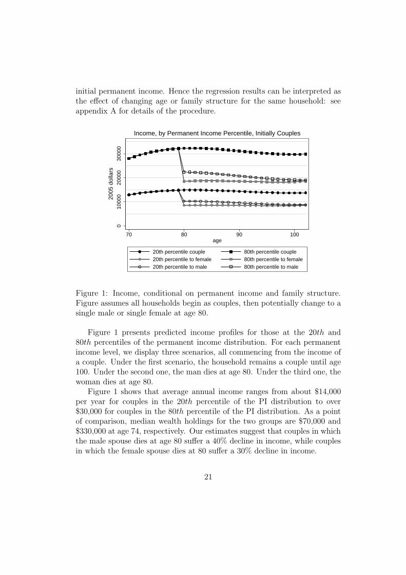
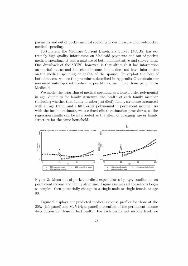
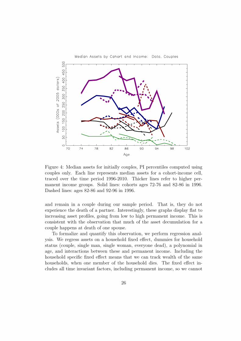
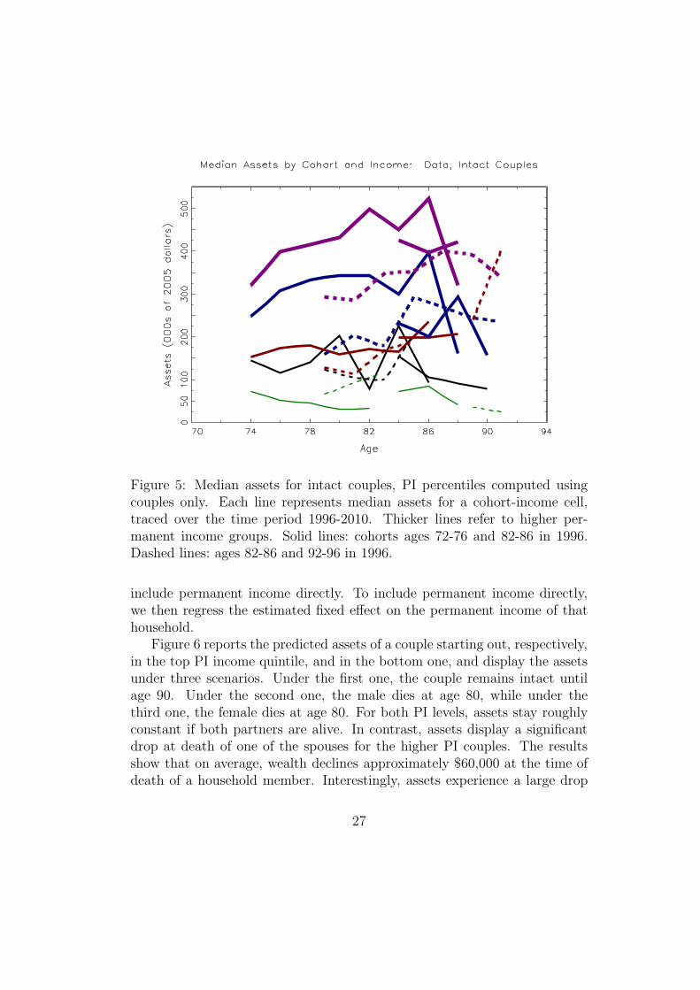
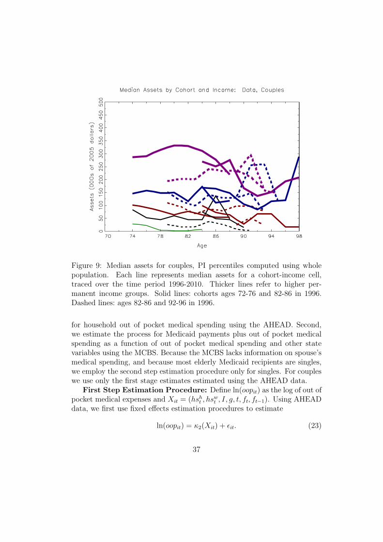
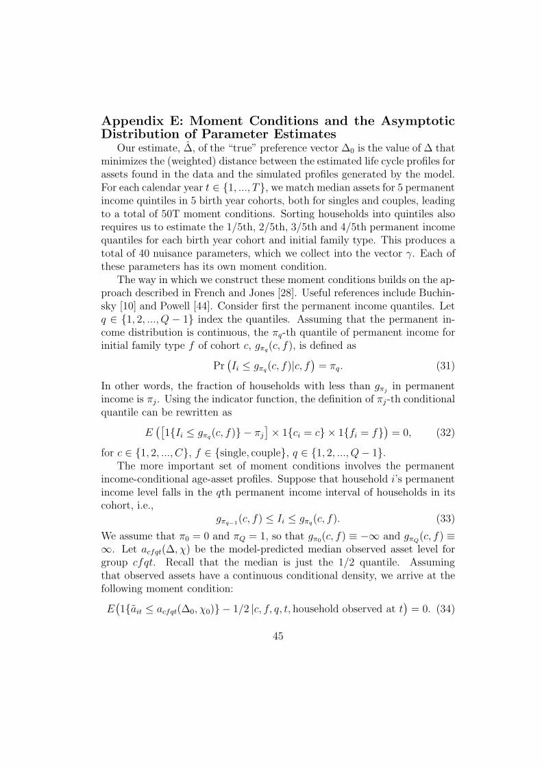
UM14-05 front pagespdf
- Couplesrsquo and Singlesrsquo Saving After Retirement
- - Mariacristina De Nardi
  - Eric French
  - John Bailey Jones
  - Couplesrsquo and Singlesrsquo Savings After Retirement
  - Abstract
  - Citation
  - - [De Nardi Mariacristina Eric French and John Bailey Jones 2015 ldquoCouples and Singlesrsquo Savings After Retirementrdquo University of Michigan Retirement Research Center (MRRC) Working Paper WP 2015-3 Ann Arbor MI httpwwwmrrcisrumichedupub
    - Authorsrsquo Acknowledgements
    - - We thank Taylor Kelley and Jeremy McCauley for excellent research assistance and the Michigan Retirement Research Center for financial support The views expressed in this paper are those of the authors and not necessarily those of the Social Security

Page 2: Couples’ and Singles’ Savings After · PDF fileWP Working Paper . 2015-322. Couples’ and Singles’ Savings After Retirement . Mariacristina De Nardi, Eric French, and John Bailey

Couplesrsquo and Singlesrsquo Saving After Retirement

Mariacristina De Nardi University College of London Federal Reserve Bank of Chicago

Institute for Fiscal Studies and NBER

Eric French University College of London Federal Reserve Bank of Chicago

and Institute for Fiscal Studies

John Bailey Jones SUNY-Albany

July 2015

Michigan Retirement Research Center University of Michigan

PO Box 1248 Ann Arbor MI 48104

wwwmrrcisrumichedu (734) 615-0422

Acknowledgements This work was supported by a grant from the Social Security Administration through the Michigan Retirement Research Center (Grant RRC08098401) The findings and conclusions expressed are solely those of the authors and do not represent the views of the Social Security Administration any agency of the federal government or the Michigan Retirement Research Center

Regents of the University of Michigan Michael J Behm Grand Blanc Mark J Bernstein Ann Arbor Laurence B Deitch Bloomfield Hills Shauna Ryder Diggs Grosse Pointe Denise Ilitch Bingham Farms Andrea Fischer Newman Ann Arbor Andrew C Richner Grosse Pointe Park Katherine E White Ann Arbor Mark S Schlissel ex officio

Abstract

Citation

1 Introduction

2

3

4

5

3 The Model

6

31 Preferences

1 νminus (1)

1 νminus (2)

7

θj(b) = φj

(b+ kj)(1minusν)

1 ν (3)

8

ψt = ζt + ξt ξt N(0 σ2ξ ) (7)

9

(11)

xt+1 = xt+1 + trt+1(xt+1 hst+1) (13)

ctxt+1

( )

(15)

minus minus

10

uc

V ct (xt hs

ht hs

wt I ζt) = max

ctxt+1bwbh(ct hs

ht hs

wt )

(V ct+1(xt+1 hs

ht+1 hs

wt+1 I ζt+1)

)

(V wt+1(x

wt+1 hs

wt+1 I ζt+1)

)+ θ1(b

ht )]

[Et

(V ht+1(x

ht+1 hs

ht+1 I ζt+1)

)+ θ1(b

wt )]+

(16)

∆ = (β ν δ ω φ0 φ1 φ2 k0 k1 k2)

11

12

ht hs

wt ζt)

13

5 Data

14

15

6 Results

16

BadHealth

GoodHealth

NursingHome

BadHealth

GoodHealth All

IncomePercentile

10 286 672 845 379 1113 1321 114630 286 730 936 378 1178 1403 122050 286 799 1034 378 1248 1489 130170 288 883 1137 378 1333 1576 138590 290 976 1244 385 1414 1654 1473

17

BadHealth

GoodHealth

NursingHome

BadHealth

GoodHealth All

IncomePercentile

10 265 688 846 359 1147 1349 104830 269 777 974 367 1246 1468 115950 276 887 1112 376 1355 1598 128670 285 1019 1262 390 1489 1729 142390 298 1169 1422 406 1626 1855 1567

18

Males FemalesBad

HealthGoodHealth

BadHealth

GoodHealth All

IncomePercentile

10 208 215 340 356 32230 205 216 341 361 32750 203 217 341 368 32870 201 216 341 369 33190 195 215 339 369 330

19

Males FemalesBad

HealthGoodHealth

BadHealth

GoodHealth All

IncomePercentile

10 161 166 318 330 24630 166 175 323 343 25750 173 186 330 357 26570 178 194 340 364 27590 185 206 349 373 283

62 Income

20

010

000

2000

030

000

70 80 90 100age

2005

dol

lars

21

22

63 Medical Spending

a

010

000

2000

0

70 80 90 100age

2005

dol

lars

b

010

000

2000

0

70 80 90 100age

2005

dol

lars

23

24

25

26

27

010

0000

2000

0030

0000

4000

00

70 80 90 100age

2005

dol

lars

28

7 Conclusions

References

29

Review 49(2)475ndash514 2008

30

ings 99(2)110ndash115 2009

31

32

33

plimTirarrinfin1

Ti

Tisum

t=1

Ti

Tisum

t=1

T[ln yit

i t=1

34

(22)

35

36

37

38

39

40

41

ctxt+1

[ dmsum

k=1 l=1 n=1

V gt+1

)]

Subject to

)

ψt+1(l n) = ζt+1(l) + ξt+1(n)

(xt minus ct

)

βs(hst I t)sumdm

k=1

sumdζl=1

sumdξn=1Π(k l n)V

( ) ( )

42

V ct (xt hs

wt hs

ht I ζt) = max

ctxt+1bwt bht

uc(ct hsht hs

wt )+

)θ2(xt minus ct)+

(θ1(b

ht ) + ω

dmsum

k=1

dζsum

l=1

dξsum

n=1

Pr(ζt+1 = ζl|ζt)

t+1

(xwt+1(k l n) hs

wt+1(k) I ζt+1(l)

))+

(θ1(b

wt ) + ω

dmsum

k=1

dζsum

l=1

dξsum

n=1

Pr(ζt+1 = ζl|ζt)

t+1

(xht+1(k l n) hs

ht+1(k) I ζt+1(l)

))+

dmsum

kh=1

dmsum

kw=1

dζsum

l=1

dξsum

n=1

V ct+1

(xt+1(kh kw l n) hs

wt+1 hs

ht+1 I ζt+1(l)

)

(30)

yct+1 = y(c I t+ 1)

yit+1 = y(i I t+ 1)

)

wt+1(kw) t+ 1 I)

43

ψt+1(l n) = ζt+1(l) + ξt+1(n)

t mwt )

u(ct m

ht m

wt

)

ht m

wt ζt) = u

(ct m

ht m

wt

)+ βswmIts

hmIt sumC

ht m

wt ζt)

cct(xt Imht m

wt ζt) =maximizer

V ct (xt Im

ht m

wt ζt) =maximum

ht m

wt ζt)

44

( le minus |

)

Ii gπq(c f) c f =

(le |

)

(c f) is defined as

Pr πq (31)

([ ] )

(33)

45

(

argmin∆γ

I

1 + τϕI(∆ γχ0)

radicI

((∆γ

)minus(

∆0

γ0

)) N(0V)

part∆prime

∣∣∣∆=∆0

partϕ(∆ γχ0)

[ ∣ ∣ ](36)

46

I

1 + τϕI(∆ γχ0)

R = PSP

47

(36) as

part∆prime

[ ](37)

[ ( ) ]

(39)

v0

( )

( )times

(|

)

f gπq(c f) c f t|

partγprime

(40)

]f(Ii|c f)dIi = 0

( )

(41)

are given by

part∆prime (42)

( )

f(gπqminus1

(c f)

( )

]

f(gπq

(c f) t)minus 12

])prime

(43)

48

with

(c f) t 12 0| | minus equiv) [ ( ) ]( ) [ ( ) ]

(c f) t 12| | minus( )

(44)

f 0(

(45)

49

  - Eric French
  - John Bailey Jones
  - Abstract
  - Citation

Page 3: Couples’ and Singles’ Savings After · PDF fileWP Working Paper . 2015-322. Couples’ and Singles’ Savings After Retirement . Mariacristina De Nardi, Eric French, and John Bailey

Abstract

Citation

1 Introduction

2

3

4

5

3 The Model

6

31 Preferences

1 νminus (1)

1 νminus (2)

7

θj(b) = φj

(b+ kj)(1minusν)

1 ν (3)

8

ψt = ζt + ξt ξt N(0 σ2ξ ) (7)

9

(11)

xt+1 = xt+1 + trt+1(xt+1 hst+1) (13)

ctxt+1

( )

(15)

minus minus

10

uc

V ct (xt hs

ht hs

wt I ζt) = max

ctxt+1bwbh(ct hs

ht hs

wt )

(V ct+1(xt+1 hs

ht+1 hs

wt+1 I ζt+1)

)

(V wt+1(x

wt+1 hs

wt+1 I ζt+1)

)+ θ1(b

ht )]

[Et

(V ht+1(x

ht+1 hs

ht+1 I ζt+1)

)+ θ1(b

wt )]+

(16)

∆ = (β ν δ ω φ0 φ1 φ2 k0 k1 k2)

11

12

ht hs

wt ζt)

13

5 Data

14

15

6 Results

16

BadHealth

GoodHealth

NursingHome

BadHealth

GoodHealth All

IncomePercentile

10 286 672 845 379 1113 1321 114630 286 730 936 378 1178 1403 122050 286 799 1034 378 1248 1489 130170 288 883 1137 378 1333 1576 138590 290 976 1244 385 1414 1654 1473

17

BadHealth

GoodHealth

NursingHome

BadHealth

GoodHealth All

IncomePercentile

10 265 688 846 359 1147 1349 104830 269 777 974 367 1246 1468 115950 276 887 1112 376 1355 1598 128670 285 1019 1262 390 1489 1729 142390 298 1169 1422 406 1626 1855 1567

18

Males FemalesBad

HealthGoodHealth

BadHealth

GoodHealth All

IncomePercentile

10 208 215 340 356 32230 205 216 341 361 32750 203 217 341 368 32870 201 216 341 369 33190 195 215 339 369 330

19

Males FemalesBad

HealthGoodHealth

BadHealth

GoodHealth All

IncomePercentile

10 161 166 318 330 24630 166 175 323 343 25750 173 186 330 357 26570 178 194 340 364 27590 185 206 349 373 283

62 Income

20

010

000

2000

030

000

70 80 90 100age

2005

dol

lars

21

22

63 Medical Spending

a

010

000

2000

0

70 80 90 100age

2005

dol

lars

b

010

000

2000

0

70 80 90 100age

2005

dol

lars

23

24

25

26

27

010

0000

2000

0030

0000

4000

00

70 80 90 100age

2005

dol

lars

28

7 Conclusions

References

29

Review 49(2)475ndash514 2008

30

ings 99(2)110ndash115 2009

31

32

33

plimTirarrinfin1

Ti

Tisum

t=1

Ti

Tisum

t=1

T[ln yit

i t=1

34

(22)

35

36

37

38

39

40

41

ctxt+1

[ dmsum

k=1 l=1 n=1

V gt+1

)]

Subject to

)

ψt+1(l n) = ζt+1(l) + ξt+1(n)

(xt minus ct

)

βs(hst I t)sumdm

k=1

sumdζl=1

sumdξn=1Π(k l n)V

( ) ( )

42

V ct (xt hs

wt hs

ht I ζt) = max

ctxt+1bwt bht

uc(ct hsht hs

wt )+

)θ2(xt minus ct)+

(θ1(b

ht ) + ω

dmsum

k=1

dζsum

l=1

dξsum

n=1

Pr(ζt+1 = ζl|ζt)

t+1

(xwt+1(k l n) hs

wt+1(k) I ζt+1(l)

))+

(θ1(b

wt ) + ω

dmsum

k=1

dζsum

l=1

dξsum

n=1

Pr(ζt+1 = ζl|ζt)

t+1

(xht+1(k l n) hs

ht+1(k) I ζt+1(l)

))+

dmsum

kh=1

dmsum

kw=1

dζsum

l=1

dξsum

n=1

V ct+1

(xt+1(kh kw l n) hs

wt+1 hs

ht+1 I ζt+1(l)

)

(30)

yct+1 = y(c I t+ 1)

yit+1 = y(i I t+ 1)

)

wt+1(kw) t+ 1 I)

43

ψt+1(l n) = ζt+1(l) + ξt+1(n)

t mwt )

u(ct m

ht m

wt

)

ht m

wt ζt) = u

(ct m

ht m

wt

)+ βswmIts

hmIt sumC

ht m

wt ζt)

cct(xt Imht m

wt ζt) =maximizer

V ct (xt Im

ht m

wt ζt) =maximum

ht m

wt ζt)

44

( le minus |

)

Ii gπq(c f) c f =

(le |

)

(c f) is defined as

Pr πq (31)

([ ] )

(33)

45

(

argmin∆γ

I

1 + τϕI(∆ γχ0)

radicI

((∆γ

)minus(

∆0

γ0

)) N(0V)

part∆prime

∣∣∣∆=∆0

partϕ(∆ γχ0)

[ ∣ ∣ ](36)

46

I

1 + τϕI(∆ γχ0)

R = PSP

47

(36) as

part∆prime

[ ](37)

[ ( ) ]

(39)

v0

( )

( )times

(|

)

f gπq(c f) c f t|

partγprime

(40)

]f(Ii|c f)dIi = 0

( )

(41)

are given by

part∆prime (42)

( )

f(gπqminus1

(c f)

( )

]

f(gπq

(c f) t)minus 12

])prime

(43)

48

with

(c f) t 12 0| | minus equiv) [ ( ) ]( ) [ ( ) ]

(c f) t 12| | minus( )

(44)

f 0(

(45)

49

  - Eric French
  - John Bailey Jones
  - Abstract
  - Citation

Page 4: Couples’ and Singles’ Savings After · PDF fileWP Working Paper . 2015-322. Couples’ and Singles’ Savings After Retirement . Mariacristina De Nardi, Eric French, and John Bailey

1 Introduction

2

3

4

5

3 The Model

6

31 Preferences

1 νminus (1)

1 νminus (2)

7

θj(b) = φj

(b+ kj)(1minusν)

1 ν (3)

8

ψt = ζt + ξt ξt N(0 σ2ξ ) (7)

9

(11)

xt+1 = xt+1 + trt+1(xt+1 hst+1) (13)

ctxt+1

( )

(15)

minus minus

10

uc

V ct (xt hs

ht hs

wt I ζt) = max

ctxt+1bwbh(ct hs

ht hs

wt )

(V ct+1(xt+1 hs

ht+1 hs

wt+1 I ζt+1)

)

(V wt+1(x

wt+1 hs

wt+1 I ζt+1)

)+ θ1(b

ht )]

[Et

(V ht+1(x

ht+1 hs

ht+1 I ζt+1)

)+ θ1(b

wt )]+

(16)

∆ = (β ν δ ω φ0 φ1 φ2 k0 k1 k2)

11

12

ht hs

wt ζt)

13

5 Data

14

15

6 Results

16

BadHealth

GoodHealth

NursingHome

BadHealth

GoodHealth All

IncomePercentile

10 286 672 845 379 1113 1321 114630 286 730 936 378 1178 1403 122050 286 799 1034 378 1248 1489 130170 288 883 1137 378 1333 1576 138590 290 976 1244 385 1414 1654 1473

17

BadHealth

GoodHealth

NursingHome

BadHealth

GoodHealth All

IncomePercentile

10 265 688 846 359 1147 1349 104830 269 777 974 367 1246 1468 115950 276 887 1112 376 1355 1598 128670 285 1019 1262 390 1489 1729 142390 298 1169 1422 406 1626 1855 1567

18

Males FemalesBad

HealthGoodHealth

BadHealth

GoodHealth All

IncomePercentile

10 208 215 340 356 32230 205 216 341 361 32750 203 217 341 368 32870 201 216 341 369 33190 195 215 339 369 330

19

Males FemalesBad

HealthGoodHealth

BadHealth

GoodHealth All

IncomePercentile

10 161 166 318 330 24630 166 175 323 343 25750 173 186 330 357 26570 178 194 340 364 27590 185 206 349 373 283

62 Income

20

010

000

2000

030

000

70 80 90 100age

2005

dol

lars

21

22

63 Medical Spending

a

010

000

2000

0

70 80 90 100age

2005

dol

lars

b

010

000

2000

0

70 80 90 100age

2005

dol

lars

23

24

25

26

27

010

0000

2000

0030

0000

4000

00

70 80 90 100age

2005

dol

lars

28

7 Conclusions

References

29

Review 49(2)475ndash514 2008

30

ings 99(2)110ndash115 2009

31

32

33

plimTirarrinfin1

Ti

Tisum

t=1

Ti

Tisum

t=1

T[ln yit

i t=1

34

(22)

35

36

37

38

39

40

41

ctxt+1

[ dmsum

k=1 l=1 n=1

V gt+1

)]

Subject to

)

ψt+1(l n) = ζt+1(l) + ξt+1(n)

(xt minus ct

)

βs(hst I t)sumdm

k=1

sumdζl=1

sumdξn=1Π(k l n)V

( ) ( )

42

V ct (xt hs

wt hs

ht I ζt) = max

ctxt+1bwt bht

uc(ct hsht hs

wt )+

)θ2(xt minus ct)+

(θ1(b

ht ) + ω

dmsum

k=1

dζsum

l=1

dξsum

n=1

Pr(ζt+1 = ζl|ζt)

t+1

(xwt+1(k l n) hs

wt+1(k) I ζt+1(l)

))+

(θ1(b

wt ) + ω

dmsum

k=1

dζsum

l=1

dξsum

n=1

Pr(ζt+1 = ζl|ζt)

t+1

(xht+1(k l n) hs

ht+1(k) I ζt+1(l)

))+

dmsum

kh=1

dmsum

kw=1

dζsum

l=1

dξsum

n=1

V ct+1

(xt+1(kh kw l n) hs

wt+1 hs

ht+1 I ζt+1(l)

)

(30)

yct+1 = y(c I t+ 1)

yit+1 = y(i I t+ 1)

)

wt+1(kw) t+ 1 I)

43

ψt+1(l n) = ζt+1(l) + ξt+1(n)

t mwt )

u(ct m

ht m

wt

)

ht m

wt ζt) = u

(ct m

ht m

wt

)+ βswmIts

hmIt sumC

ht m

wt ζt)

cct(xt Imht m

wt ζt) =maximizer

V ct (xt Im

ht m

wt ζt) =maximum

ht m

wt ζt)

44

( le minus |

)

Ii gπq(c f) c f =

(le |

)

(c f) is defined as

Pr πq (31)

([ ] )

(33)

45

(

argmin∆γ

I

1 + τϕI(∆ γχ0)

radicI

((∆γ

)minus(

∆0

γ0

)) N(0V)

part∆prime

∣∣∣∆=∆0

partϕ(∆ γχ0)

[ ∣ ∣ ](36)

46

I

1 + τϕI(∆ γχ0)

R = PSP

47

(36) as

part∆prime

[ ](37)

[ ( ) ]

(39)

v0

( )

( )times

(|

)

f gπq(c f) c f t|

partγprime

(40)

]f(Ii|c f)dIi = 0

( )

(41)

are given by

part∆prime (42)

( )

f(gπqminus1

(c f)

( )

]

f(gπq

(c f) t)minus 12

])prime

(43)

48

with

(c f) t 12 0| | minus equiv) [ ( ) ]( ) [ ( ) ]

(c f) t 12| | minus( )

(44)

f 0(

(45)

49

  - Eric French
  - John Bailey Jones
  - Abstract
  - Citation

Page 5: Couples’ and Singles’ Savings After · PDF fileWP Working Paper . 2015-322. Couples’ and Singles’ Savings After Retirement . Mariacristina De Nardi, Eric French, and John Bailey

3

4

5

3 The Model

6

31 Preferences

1 νminus (1)

1 νminus (2)

7

θj(b) = φj

(b+ kj)(1minusν)

1 ν (3)

8

ψt = ζt + ξt ξt N(0 σ2ξ ) (7)

9

(11)

xt+1 = xt+1 + trt+1(xt+1 hst+1) (13)

ctxt+1

( )

(15)

minus minus

10

uc

V ct (xt hs

ht hs

wt I ζt) = max

ctxt+1bwbh(ct hs

ht hs

wt )

(V ct+1(xt+1 hs

ht+1 hs

wt+1 I ζt+1)

)

(V wt+1(x

wt+1 hs

wt+1 I ζt+1)

)+ θ1(b

ht )]

[Et

(V ht+1(x

ht+1 hs

ht+1 I ζt+1)

)+ θ1(b

wt )]+

(16)

∆ = (β ν δ ω φ0 φ1 φ2 k0 k1 k2)

11

12

ht hs

wt ζt)

13

5 Data

14

15

6 Results

16

BadHealth

GoodHealth

NursingHome

BadHealth

GoodHealth All

IncomePercentile

10 286 672 845 379 1113 1321 114630 286 730 936 378 1178 1403 122050 286 799 1034 378 1248 1489 130170 288 883 1137 378 1333 1576 138590 290 976 1244 385 1414 1654 1473

17

BadHealth

GoodHealth

NursingHome

BadHealth

GoodHealth All

IncomePercentile

10 265 688 846 359 1147 1349 104830 269 777 974 367 1246 1468 115950 276 887 1112 376 1355 1598 128670 285 1019 1262 390 1489 1729 142390 298 1169 1422 406 1626 1855 1567

18

Males FemalesBad

HealthGoodHealth

BadHealth

GoodHealth All

IncomePercentile

10 208 215 340 356 32230 205 216 341 361 32750 203 217 341 368 32870 201 216 341 369 33190 195 215 339 369 330

19

Males FemalesBad

HealthGoodHealth

BadHealth

GoodHealth All

IncomePercentile

10 161 166 318 330 24630 166 175 323 343 25750 173 186 330 357 26570 178 194 340 364 27590 185 206 349 373 283

62 Income

20

010

000

2000

030

000

70 80 90 100age

2005

dol

lars

21

22

63 Medical Spending

a

010

000

2000

0

70 80 90 100age

2005

dol

lars

b

010

000

2000

0

70 80 90 100age

2005

dol

lars

23

24

25

26

27

010

0000

2000

0030

0000

4000

00

70 80 90 100age

2005

dol

lars

28

7 Conclusions

References

29

Review 49(2)475ndash514 2008

30

ings 99(2)110ndash115 2009

31

32

33

plimTirarrinfin1

Ti

Tisum

t=1

Ti

Tisum

t=1

T[ln yit

i t=1

34

(22)

35

36

37

38

39

40

41

ctxt+1

[ dmsum

k=1 l=1 n=1

V gt+1

)]

Subject to

)

ψt+1(l n) = ζt+1(l) + ξt+1(n)

(xt minus ct

)

βs(hst I t)sumdm

k=1

sumdζl=1

sumdξn=1Π(k l n)V

( ) ( )

42

V ct (xt hs

wt hs

ht I ζt) = max

ctxt+1bwt bht

uc(ct hsht hs

wt )+

)θ2(xt minus ct)+

(θ1(b

ht ) + ω

dmsum

k=1

dζsum

l=1

dξsum

n=1

Pr(ζt+1 = ζl|ζt)

t+1

(xwt+1(k l n) hs

wt+1(k) I ζt+1(l)

))+

(θ1(b

wt ) + ω

dmsum

k=1

dζsum

l=1

dξsum

n=1

Pr(ζt+1 = ζl|ζt)

t+1

(xht+1(k l n) hs

ht+1(k) I ζt+1(l)

))+

dmsum

kh=1

dmsum

kw=1

dζsum

l=1

dξsum

n=1

V ct+1

(xt+1(kh kw l n) hs

wt+1 hs

ht+1 I ζt+1(l)

)

(30)

yct+1 = y(c I t+ 1)

yit+1 = y(i I t+ 1)

)

wt+1(kw) t+ 1 I)

43

ψt+1(l n) = ζt+1(l) + ξt+1(n)

t mwt )

u(ct m

ht m

wt

)

ht m

wt ζt) = u

(ct m

ht m

wt

)+ βswmIts

hmIt sumC

ht m

wt ζt)

cct(xt Imht m

wt ζt) =maximizer

V ct (xt Im

ht m

wt ζt) =maximum

ht m

wt ζt)

44

( le minus |

)

Ii gπq(c f) c f =

(le |

)

(c f) is defined as

Pr πq (31)

([ ] )

(33)

45

(

argmin∆γ

I

1 + τϕI(∆ γχ0)

radicI

((∆γ

)minus(

∆0

γ0

)) N(0V)

part∆prime

∣∣∣∆=∆0

partϕ(∆ γχ0)

[ ∣ ∣ ](36)

46

I

1 + τϕI(∆ γχ0)

R = PSP

47

(36) as

part∆prime

[ ](37)

[ ( ) ]

(39)

v0

( )

( )times

(|

)

f gπq(c f) c f t|

partγprime

(40)

]f(Ii|c f)dIi = 0

( )

(41)

are given by

part∆prime (42)

( )

f(gπqminus1

(c f)

( )

]

f(gπq

(c f) t)minus 12

])prime

(43)

48

with

(c f) t 12 0| | minus equiv) [ ( ) ]( ) [ ( ) ]

(c f) t 12| | minus( )

(44)

f 0(

(45)

49

  - Eric French
  - John Bailey Jones
  - Abstract
  - Citation

Page 6: Couples’ and Singles’ Savings After · PDF fileWP Working Paper . 2015-322. Couples’ and Singles’ Savings After Retirement . Mariacristina De Nardi, Eric French, and John Bailey

4

5

3 The Model

6

31 Preferences

1 νminus (1)

1 νminus (2)

7

θj(b) = φj

(b+ kj)(1minusν)

1 ν (3)

8

ψt = ζt + ξt ξt N(0 σ2ξ ) (7)

9

(11)

xt+1 = xt+1 + trt+1(xt+1 hst+1) (13)

ctxt+1

( )

(15)

minus minus

10

uc

V ct (xt hs

ht hs

wt I ζt) = max

ctxt+1bwbh(ct hs

ht hs

wt )

(V ct+1(xt+1 hs

ht+1 hs

wt+1 I ζt+1)

)

(V wt+1(x

wt+1 hs

wt+1 I ζt+1)

)+ θ1(b

ht )]

[Et

(V ht+1(x

ht+1 hs

ht+1 I ζt+1)

)+ θ1(b

wt )]+

(16)

∆ = (β ν δ ω φ0 φ1 φ2 k0 k1 k2)

11

12

ht hs

wt ζt)

13

5 Data

14

15

6 Results

16

BadHealth

GoodHealth

NursingHome

BadHealth

GoodHealth All

IncomePercentile

10 286 672 845 379 1113 1321 114630 286 730 936 378 1178 1403 122050 286 799 1034 378 1248 1489 130170 288 883 1137 378 1333 1576 138590 290 976 1244 385 1414 1654 1473

17

BadHealth

GoodHealth

NursingHome

BadHealth

GoodHealth All

IncomePercentile

10 265 688 846 359 1147 1349 104830 269 777 974 367 1246 1468 115950 276 887 1112 376 1355 1598 128670 285 1019 1262 390 1489 1729 142390 298 1169 1422 406 1626 1855 1567

18

Males FemalesBad

HealthGoodHealth

BadHealth

GoodHealth All

IncomePercentile

10 208 215 340 356 32230 205 216 341 361 32750 203 217 341 368 32870 201 216 341 369 33190 195 215 339 369 330

19

Males FemalesBad

HealthGoodHealth

BadHealth

GoodHealth All

IncomePercentile

10 161 166 318 330 24630 166 175 323 343 25750 173 186 330 357 26570 178 194 340 364 27590 185 206 349 373 283

62 Income

20

010

000

2000

030

000

70 80 90 100age

2005

dol

lars

21

22

63 Medical Spending

a

010

000

2000

0

70 80 90 100age

2005

dol

lars

b

010

000

2000

0

70 80 90 100age

2005

dol

lars

23

24

25

26

27

010

0000

2000

0030

0000

4000

00

70 80 90 100age

2005

dol

lars

28

7 Conclusions

References

29

Review 49(2)475ndash514 2008

30

ings 99(2)110ndash115 2009

31

32

33

plimTirarrinfin1

Ti

Tisum

t=1

Ti

Tisum

t=1

T[ln yit

i t=1

34

(22)

35

36

37

38

39

40

41

ctxt+1

[ dmsum

k=1 l=1 n=1

V gt+1

)]

Subject to

)

ψt+1(l n) = ζt+1(l) + ξt+1(n)

(xt minus ct

)

βs(hst I t)sumdm

k=1

sumdζl=1

sumdξn=1Π(k l n)V

( ) ( )

42

V ct (xt hs

wt hs

ht I ζt) = max

ctxt+1bwt bht

uc(ct hsht hs

wt )+

)θ2(xt minus ct)+

(θ1(b

ht ) + ω

dmsum

k=1

dζsum

l=1

dξsum

n=1

Pr(ζt+1 = ζl|ζt)

t+1

(xwt+1(k l n) hs

wt+1(k) I ζt+1(l)

))+

(θ1(b

wt ) + ω

dmsum

k=1

dζsum

l=1

dξsum

n=1

Pr(ζt+1 = ζl|ζt)

t+1

(xht+1(k l n) hs

ht+1(k) I ζt+1(l)

))+

dmsum

kh=1

dmsum

kw=1

dζsum

l=1

dξsum

n=1

V ct+1

(xt+1(kh kw l n) hs

wt+1 hs

ht+1 I ζt+1(l)

)

(30)

yct+1 = y(c I t+ 1)

yit+1 = y(i I t+ 1)

)

wt+1(kw) t+ 1 I)

43

ψt+1(l n) = ζt+1(l) + ξt+1(n)

t mwt )

u(ct m

ht m

wt

)

ht m

wt ζt) = u

(ct m

ht m

wt

)+ βswmIts

hmIt sumC

ht m

wt ζt)

cct(xt Imht m

wt ζt) =maximizer

V ct (xt Im

ht m

wt ζt) =maximum

ht m

wt ζt)

44

( le minus |

)

Ii gπq(c f) c f =

(le |

)

(c f) is defined as

Pr πq (31)

([ ] )

(33)

45

(

argmin∆γ

I

1 + τϕI(∆ γχ0)

radicI

((∆γ

)minus(

∆0

γ0

)) N(0V)

part∆prime

∣∣∣∆=∆0

partϕ(∆ γχ0)

[ ∣ ∣ ](36)

46

I

1 + τϕI(∆ γχ0)

R = PSP

47

(36) as

part∆prime

[ ](37)

[ ( ) ]

(39)

v0

( )

( )times

(|

)

f gπq(c f) c f t|

partγprime

(40)

]f(Ii|c f)dIi = 0

( )

(41)

are given by

part∆prime (42)

( )

f(gπqminus1

(c f)

( )

]

f(gπq

(c f) t)minus 12

])prime

(43)

48

with

(c f) t 12 0| | minus equiv) [ ( ) ]( ) [ ( ) ]

(c f) t 12| | minus( )

(44)

f 0(

(45)

49

  - Eric French
  - John Bailey Jones
  - Abstract
  - Citation

Page 7: Couples’ and Singles’ Savings After · PDF fileWP Working Paper . 2015-322. Couples’ and Singles’ Savings After Retirement . Mariacristina De Nardi, Eric French, and John Bailey

5

3 The Model

6

31 Preferences

1 νminus (1)

1 νminus (2)

7

θj(b) = φj

(b+ kj)(1minusν)

1 ν (3)

8

ψt = ζt + ξt ξt N(0 σ2ξ ) (7)

9

(11)

xt+1 = xt+1 + trt+1(xt+1 hst+1) (13)

ctxt+1

( )

(15)

minus minus

10

uc

V ct (xt hs

ht hs

wt I ζt) = max

ctxt+1bwbh(ct hs

ht hs

wt )

(V ct+1(xt+1 hs

ht+1 hs

wt+1 I ζt+1)

)

(V wt+1(x

wt+1 hs

wt+1 I ζt+1)

)+ θ1(b

ht )]

[Et

(V ht+1(x

ht+1 hs

ht+1 I ζt+1)

)+ θ1(b

wt )]+

(16)

∆ = (β ν δ ω φ0 φ1 φ2 k0 k1 k2)

11

12

ht hs

wt ζt)

13

5 Data

14

15

6 Results

16

BadHealth

GoodHealth

NursingHome

BadHealth

GoodHealth All

IncomePercentile

10 286 672 845 379 1113 1321 114630 286 730 936 378 1178 1403 122050 286 799 1034 378 1248 1489 130170 288 883 1137 378 1333 1576 138590 290 976 1244 385 1414 1654 1473

17

BadHealth

GoodHealth

NursingHome

BadHealth

GoodHealth All

IncomePercentile

10 265 688 846 359 1147 1349 104830 269 777 974 367 1246 1468 115950 276 887 1112 376 1355 1598 128670 285 1019 1262 390 1489 1729 142390 298 1169 1422 406 1626 1855 1567

18

Males FemalesBad

HealthGoodHealth

BadHealth

GoodHealth All

IncomePercentile

10 208 215 340 356 32230 205 216 341 361 32750 203 217 341 368 32870 201 216 341 369 33190 195 215 339 369 330

19

Males FemalesBad

HealthGoodHealth

BadHealth

GoodHealth All

IncomePercentile

10 161 166 318 330 24630 166 175 323 343 25750 173 186 330 357 26570 178 194 340 364 27590 185 206 349 373 283

62 Income

20

010

000

2000

030

000

70 80 90 100age

2005

dol

lars

21

22

63 Medical Spending

a

010

000

2000

0

70 80 90 100age

2005

dol

lars

b

010

000

2000

0

70 80 90 100age

2005

dol

lars

23

24

25

26

27

010

0000

2000

0030

0000

4000

00

70 80 90 100age

2005

dol

lars

28

7 Conclusions

References

29

Review 49(2)475ndash514 2008

30

ings 99(2)110ndash115 2009

31

32

33

plimTirarrinfin1

Ti

Tisum

t=1

Ti

Tisum

t=1

T[ln yit

i t=1

34

(22)

35

36

37

38

39

40

41

ctxt+1

[ dmsum

k=1 l=1 n=1

V gt+1

)]

Subject to

)

ψt+1(l n) = ζt+1(l) + ξt+1(n)

(xt minus ct

)

βs(hst I t)sumdm

k=1

sumdζl=1

sumdξn=1Π(k l n)V

( ) ( )

42

V ct (xt hs

wt hs

ht I ζt) = max

ctxt+1bwt bht

uc(ct hsht hs

wt )+

)θ2(xt minus ct)+

(θ1(b

ht ) + ω

dmsum

k=1

dζsum

l=1

dξsum

n=1

Pr(ζt+1 = ζl|ζt)

t+1

(xwt+1(k l n) hs

wt+1(k) I ζt+1(l)

))+

(θ1(b

wt ) + ω

dmsum

k=1

dζsum

l=1

dξsum

n=1

Pr(ζt+1 = ζl|ζt)

t+1

(xht+1(k l n) hs

ht+1(k) I ζt+1(l)

))+

dmsum

kh=1

dmsum

kw=1

dζsum

l=1

dξsum

n=1

V ct+1

(xt+1(kh kw l n) hs

wt+1 hs

ht+1 I ζt+1(l)

)

(30)

yct+1 = y(c I t+ 1)

yit+1 = y(i I t+ 1)

)

wt+1(kw) t+ 1 I)

43

ψt+1(l n) = ζt+1(l) + ξt+1(n)

t mwt )

u(ct m

ht m

wt

)

ht m

wt ζt) = u

(ct m

ht m

wt

)+ βswmIts

hmIt sumC

ht m

wt ζt)

cct(xt Imht m

wt ζt) =maximizer

V ct (xt Im

ht m

wt ζt) =maximum

ht m

wt ζt)

44

( le minus |

)

Ii gπq(c f) c f =

(le |

)

(c f) is defined as

Pr πq (31)

([ ] )

(33)

45

(

argmin∆γ

I

1 + τϕI(∆ γχ0)

radicI

((∆γ

)minus(

∆0

γ0

)) N(0V)

part∆prime

∣∣∣∆=∆0

partϕ(∆ γχ0)

[ ∣ ∣ ](36)

46

I

1 + τϕI(∆ γχ0)

R = PSP

47

(36) as

part∆prime

[ ](37)

[ ( ) ]

(39)

v0

( )

( )times

(|

)

f gπq(c f) c f t|

partγprime

(40)

]f(Ii|c f)dIi = 0

( )

(41)

are given by

part∆prime (42)

( )

f(gπqminus1

(c f)

( )

]

f(gπq

(c f) t)minus 12

])prime

(43)

48

with

(c f) t 12 0| | minus equiv) [ ( ) ]( ) [ ( ) ]

(c f) t 12| | minus( )

(44)

f 0(

(45)

49

  - Eric French
  - John Bailey Jones
  - Abstract
  - Citation

Page 8: Couples’ and Singles’ Savings After · PDF fileWP Working Paper . 2015-322. Couples’ and Singles’ Savings After Retirement . Mariacristina De Nardi, Eric French, and John Bailey

3 The Model

6

31 Preferences

1 νminus (1)

1 νminus (2)

7

θj(b) = φj

(b+ kj)(1minusν)

1 ν (3)

8

ψt = ζt + ξt ξt N(0 σ2ξ ) (7)

9

(11)

xt+1 = xt+1 + trt+1(xt+1 hst+1) (13)

ctxt+1

( )

(15)

minus minus

10

uc

V ct (xt hs

ht hs

wt I ζt) = max

ctxt+1bwbh(ct hs

ht hs

wt )

(V ct+1(xt+1 hs

ht+1 hs

wt+1 I ζt+1)

)

(V wt+1(x

wt+1 hs

wt+1 I ζt+1)

)+ θ1(b

ht )]

[Et

(V ht+1(x

ht+1 hs

ht+1 I ζt+1)

)+ θ1(b

wt )]+

(16)

∆ = (β ν δ ω φ0 φ1 φ2 k0 k1 k2)

11

12

ht hs

wt ζt)

13

5 Data

14

15

6 Results

16

BadHealth

GoodHealth

NursingHome

BadHealth

GoodHealth All

IncomePercentile

10 286 672 845 379 1113 1321 114630 286 730 936 378 1178 1403 122050 286 799 1034 378 1248 1489 130170 288 883 1137 378 1333 1576 138590 290 976 1244 385 1414 1654 1473

17

BadHealth

GoodHealth

NursingHome

BadHealth

GoodHealth All

IncomePercentile

10 265 688 846 359 1147 1349 104830 269 777 974 367 1246 1468 115950 276 887 1112 376 1355 1598 128670 285 1019 1262 390 1489 1729 142390 298 1169 1422 406 1626 1855 1567

18

Males FemalesBad

HealthGoodHealth

BadHealth

GoodHealth All

IncomePercentile

10 208 215 340 356 32230 205 216 341 361 32750 203 217 341 368 32870 201 216 341 369 33190 195 215 339 369 330

19

Males FemalesBad

HealthGoodHealth

BadHealth

GoodHealth All

IncomePercentile

10 161 166 318 330 24630 166 175 323 343 25750 173 186 330 357 26570 178 194 340 364 27590 185 206 349 373 283

62 Income

20

010

000

2000

030

000

70 80 90 100age

2005

dol

lars

21

22

63 Medical Spending

a

010

000

2000

0

70 80 90 100age

2005

dol

lars

b

010

000

2000

0

70 80 90 100age

2005

dol

lars

23

24

25

26

27

010

0000

2000

0030

0000

4000

00

70 80 90 100age

2005

dol

lars

28

7 Conclusions

References

29

Review 49(2)475ndash514 2008

30

ings 99(2)110ndash115 2009

31

32

33

plimTirarrinfin1

Ti

Tisum

t=1

Ti

Tisum

t=1

T[ln yit

i t=1

34

(22)

35

36

37

38

39

40

41

ctxt+1

[ dmsum

k=1 l=1 n=1

V gt+1

)]

Subject to

)

ψt+1(l n) = ζt+1(l) + ξt+1(n)

(xt minus ct

)

βs(hst I t)sumdm

k=1

sumdζl=1

sumdξn=1Π(k l n)V

( ) ( )

42

V ct (xt hs

wt hs

ht I ζt) = max

ctxt+1bwt bht

uc(ct hsht hs

wt )+

)θ2(xt minus ct)+

(θ1(b

ht ) + ω

dmsum

k=1

dζsum

l=1

dξsum

n=1

Pr(ζt+1 = ζl|ζt)

t+1

(xwt+1(k l n) hs

wt+1(k) I ζt+1(l)

))+

(θ1(b

wt ) + ω

dmsum

k=1

dζsum

l=1

dξsum

n=1

Pr(ζt+1 = ζl|ζt)

t+1

(xht+1(k l n) hs

ht+1(k) I ζt+1(l)

))+

dmsum

kh=1

dmsum

kw=1

dζsum

l=1

dξsum

n=1

V ct+1

(xt+1(kh kw l n) hs

wt+1 hs

ht+1 I ζt+1(l)

)

(30)

yct+1 = y(c I t+ 1)

yit+1 = y(i I t+ 1)

)

wt+1(kw) t+ 1 I)

43

ψt+1(l n) = ζt+1(l) + ξt+1(n)

t mwt )

u(ct m

ht m

wt

)

ht m

wt ζt) = u

(ct m

ht m

wt

)+ βswmIts

hmIt sumC

ht m

wt ζt)

cct(xt Imht m

wt ζt) =maximizer

V ct (xt Im

ht m

wt ζt) =maximum

ht m

wt ζt)

44

( le minus |

)

Ii gπq(c f) c f =

(le |

)

(c f) is defined as

Pr πq (31)

([ ] )

(33)

45

(

argmin∆γ

I

1 + τϕI(∆ γχ0)

radicI

((∆γ

)minus(

∆0

γ0

)) N(0V)

part∆prime

∣∣∣∆=∆0

partϕ(∆ γχ0)

[ ∣ ∣ ](36)

46

I

1 + τϕI(∆ γχ0)

R = PSP

47

(36) as

part∆prime

[ ](37)

[ ( ) ]

(39)

v0

( )

( )times

(|

)

f gπq(c f) c f t|

partγprime

(40)

]f(Ii|c f)dIi = 0

( )

(41)

are given by

part∆prime (42)

( )

f(gπqminus1

(c f)

( )

]

f(gπq

(c f) t)minus 12

])prime

(43)

48

with

(c f) t 12 0| | minus equiv) [ ( ) ]( ) [ ( ) ]

(c f) t 12| | minus( )

(44)

f 0(

(45)

49

  - Eric French
  - John Bailey Jones
  - Abstract
  - Citation

Page 9: Couples’ and Singles’ Savings After · PDF fileWP Working Paper . 2015-322. Couples’ and Singles’ Savings After Retirement . Mariacristina De Nardi, Eric French, and John Bailey

31 Preferences

1 νminus (1)

1 νminus (2)

7

θj(b) = φj

(b+ kj)(1minusν)

1 ν (3)

8

ψt = ζt + ξt ξt N(0 σ2ξ ) (7)

9

(11)

xt+1 = xt+1 + trt+1(xt+1 hst+1) (13)

ctxt+1

( )

(15)

minus minus

10

uc

V ct (xt hs

ht hs

wt I ζt) = max

ctxt+1bwbh(ct hs

ht hs

wt )

(V ct+1(xt+1 hs

ht+1 hs

wt+1 I ζt+1)

)

(V wt+1(x

wt+1 hs

wt+1 I ζt+1)

)+ θ1(b

ht )]

[Et

(V ht+1(x

ht+1 hs

ht+1 I ζt+1)

)+ θ1(b

wt )]+

(16)

∆ = (β ν δ ω φ0 φ1 φ2 k0 k1 k2)

11

12

ht hs

wt ζt)

13

5 Data

14

15

6 Results

16

BadHealth

GoodHealth

NursingHome

BadHealth

GoodHealth All

IncomePercentile

10 286 672 845 379 1113 1321 114630 286 730 936 378 1178 1403 122050 286 799 1034 378 1248 1489 130170 288 883 1137 378 1333 1576 138590 290 976 1244 385 1414 1654 1473

17

BadHealth

GoodHealth

NursingHome

BadHealth

GoodHealth All

IncomePercentile

10 265 688 846 359 1147 1349 104830 269 777 974 367 1246 1468 115950 276 887 1112 376 1355 1598 128670 285 1019 1262 390 1489 1729 142390 298 1169 1422 406 1626 1855 1567

18

Males FemalesBad

HealthGoodHealth

BadHealth

GoodHealth All

IncomePercentile

10 208 215 340 356 32230 205 216 341 361 32750 203 217 341 368 32870 201 216 341 369 33190 195 215 339 369 330

19

Males FemalesBad

HealthGoodHealth

BadHealth

GoodHealth All

IncomePercentile

10 161 166 318 330 24630 166 175 323 343 25750 173 186 330 357 26570 178 194 340 364 27590 185 206 349 373 283

62 Income

20

010

000

2000

030

000

70 80 90 100age

2005

dol

lars

21

22

63 Medical Spending

a

010

000

2000

0

70 80 90 100age

2005

dol

lars

b

010

000

2000

0

70 80 90 100age

2005

dol

lars

23

24

25

26

27

010

0000

2000

0030

0000

4000

00

70 80 90 100age

2005

dol

lars

28

7 Conclusions

References

29

Review 49(2)475ndash514 2008

30

ings 99(2)110ndash115 2009

31

32

33

plimTirarrinfin1

Ti

Tisum

t=1

Ti

Tisum

t=1

T[ln yit

i t=1

34

(22)

35

36

37

38

39

40

41

ctxt+1

[ dmsum

k=1 l=1 n=1

V gt+1

)]

Subject to

)

ψt+1(l n) = ζt+1(l) + ξt+1(n)

(xt minus ct

)

βs(hst I t)sumdm

k=1

sumdζl=1

sumdξn=1Π(k l n)V

( ) ( )

42

V ct (xt hs

wt hs

ht I ζt) = max

ctxt+1bwt bht

uc(ct hsht hs

wt )+

)θ2(xt minus ct)+

(θ1(b

ht ) + ω

dmsum

k=1

dζsum

l=1

dξsum

n=1

Pr(ζt+1 = ζl|ζt)

t+1

(xwt+1(k l n) hs

wt+1(k) I ζt+1(l)

))+

(θ1(b

wt ) + ω

dmsum

k=1

dζsum

l=1

dξsum

n=1

Pr(ζt+1 = ζl|ζt)

t+1

(xht+1(k l n) hs

ht+1(k) I ζt+1(l)

))+

dmsum

kh=1

dmsum

kw=1

dζsum

l=1

dξsum

n=1

V ct+1

(xt+1(kh kw l n) hs

wt+1 hs

ht+1 I ζt+1(l)

)

(30)

yct+1 = y(c I t+ 1)

yit+1 = y(i I t+ 1)

)

wt+1(kw) t+ 1 I)

43

ψt+1(l n) = ζt+1(l) + ξt+1(n)

t mwt )

u(ct m

ht m

wt

)

ht m

wt ζt) = u

(ct m

ht m

wt

)+ βswmIts

hmIt sumC

ht m

wt ζt)

cct(xt Imht m

wt ζt) =maximizer

V ct (xt Im

ht m

wt ζt) =maximum

ht m

wt ζt)

44

( le minus |

)

Ii gπq(c f) c f =

(le |

)

(c f) is defined as

Pr πq (31)

([ ] )

(33)

45

(

argmin∆γ

I

1 + τϕI(∆ γχ0)

radicI

((∆γ

)minus(

∆0

γ0

)) N(0V)

part∆prime

∣∣∣∆=∆0

partϕ(∆ γχ0)

[ ∣ ∣ ](36)

46

I

1 + τϕI(∆ γχ0)

R = PSP

47

(36) as

part∆prime

[ ](37)

[ ( ) ]

(39)

v0

( )

( )times

(|

)

f gπq(c f) c f t|

partγprime

(40)

]f(Ii|c f)dIi = 0

( )

(41)

are given by

part∆prime (42)

( )

f(gπqminus1

(c f)

( )

]

f(gπq

(c f) t)minus 12

])prime

(43)

48

with

(c f) t 12 0| | minus equiv) [ ( ) ]( ) [ ( ) ]

(c f) t 12| | minus( )

(44)

f 0(

(45)

49

  - Eric French
  - John Bailey Jones
  - Abstract
  - Citation

Page 10: Couples’ and Singles’ Savings After · PDF fileWP Working Paper . 2015-322. Couples’ and Singles’ Savings After Retirement . Mariacristina De Nardi, Eric French, and John Bailey

θj(b) = φj

(b+ kj)(1minusν)

1 ν (3)

8

ψt = ζt + ξt ξt N(0 σ2ξ ) (7)

9

(11)

xt+1 = xt+1 + trt+1(xt+1 hst+1) (13)

ctxt+1

( )

(15)

minus minus

10

uc

V ct (xt hs

ht hs

wt I ζt) = max

ctxt+1bwbh(ct hs

ht hs

wt )

(V ct+1(xt+1 hs

ht+1 hs

wt+1 I ζt+1)

)

(V wt+1(x

wt+1 hs

wt+1 I ζt+1)

)+ θ1(b

ht )]

[Et

(V ht+1(x

ht+1 hs

ht+1 I ζt+1)

)+ θ1(b

wt )]+

(16)

∆ = (β ν δ ω φ0 φ1 φ2 k0 k1 k2)

11

12

ht hs

wt ζt)

13

5 Data

14

15

6 Results

16

BadHealth

GoodHealth

NursingHome

BadHealth

GoodHealth All

IncomePercentile

10 286 672 845 379 1113 1321 114630 286 730 936 378 1178 1403 122050 286 799 1034 378 1248 1489 130170 288 883 1137 378 1333 1576 138590 290 976 1244 385 1414 1654 1473

17

BadHealth

GoodHealth

NursingHome

BadHealth

GoodHealth All

IncomePercentile

10 265 688 846 359 1147 1349 104830 269 777 974 367 1246 1468 115950 276 887 1112 376 1355 1598 128670 285 1019 1262 390 1489 1729 142390 298 1169 1422 406 1626 1855 1567

18

Males FemalesBad

HealthGoodHealth

BadHealth

GoodHealth All

IncomePercentile

10 208 215 340 356 32230 205 216 341 361 32750 203 217 341 368 32870 201 216 341 369 33190 195 215 339 369 330

19

Males FemalesBad

HealthGoodHealth

BadHealth

GoodHealth All

IncomePercentile

10 161 166 318 330 24630 166 175 323 343 25750 173 186 330 357 26570 178 194 340 364 27590 185 206 349 373 283

62 Income

20

010

000

2000

030

000

70 80 90 100age

2005

dol

lars

21

22

63 Medical Spending

a

010

000

2000

0

70 80 90 100age

2005

dol

lars

b

010

000

2000

0

70 80 90 100age

2005

dol

lars

23

24

25

26

27

010

0000

2000

0030

0000

4000

00

70 80 90 100age

2005

dol

lars

28

7 Conclusions

References

29

Review 49(2)475ndash514 2008

30

ings 99(2)110ndash115 2009

31

32

33

plimTirarrinfin1

Ti

Tisum

t=1

Ti

Tisum

t=1

T[ln yit

i t=1

34

(22)

35

36

37

38

39

40

41

ctxt+1

[ dmsum

k=1 l=1 n=1

V gt+1

)]

Subject to

)

ψt+1(l n) = ζt+1(l) + ξt+1(n)

(xt minus ct

)

βs(hst I t)sumdm

k=1

sumdζl=1

sumdξn=1Π(k l n)V

( ) ( )

42

V ct (xt hs

wt hs

ht I ζt) = max

ctxt+1bwt bht

uc(ct hsht hs

wt )+

)θ2(xt minus ct)+

(θ1(b

ht ) + ω

dmsum

k=1

dζsum

l=1

dξsum

n=1

Pr(ζt+1 = ζl|ζt)

t+1

(xwt+1(k l n) hs

wt+1(k) I ζt+1(l)

))+

(θ1(b

wt ) + ω

dmsum

k=1

dζsum

l=1

dξsum

n=1

Pr(ζt+1 = ζl|ζt)

t+1

(xht+1(k l n) hs

ht+1(k) I ζt+1(l)

))+

dmsum

kh=1

dmsum

kw=1

dζsum

l=1

dξsum

n=1

V ct+1

(xt+1(kh kw l n) hs

wt+1 hs

ht+1 I ζt+1(l)

)

(30)

yct+1 = y(c I t+ 1)

yit+1 = y(i I t+ 1)

)

wt+1(kw) t+ 1 I)

43

ψt+1(l n) = ζt+1(l) + ξt+1(n)

t mwt )

u(ct m

ht m

wt

)

ht m

wt ζt) = u

(ct m

ht m

wt

)+ βswmIts

hmIt sumC

ht m

wt ζt)

cct(xt Imht m

wt ζt) =maximizer

V ct (xt Im

ht m

wt ζt) =maximum

ht m

wt ζt)

44

( le minus |

)

Ii gπq(c f) c f =

(le |

)

(c f) is defined as

Pr πq (31)

([ ] )

(33)

45

(

argmin∆γ

I

1 + τϕI(∆ γχ0)

radicI

((∆γ

)minus(

∆0

γ0

)) N(0V)

part∆prime

∣∣∣∆=∆0

partϕ(∆ γχ0)

[ ∣ ∣ ](36)

46

I

1 + τϕI(∆ γχ0)

R = PSP

47

(36) as

part∆prime

[ ](37)

[ ( ) ]

(39)

v0

( )

( )times

(|

)

f gπq(c f) c f t|

partγprime

(40)

]f(Ii|c f)dIi = 0

( )

(41)

are given by

part∆prime (42)

( )

f(gπqminus1

(c f)

( )

]

f(gπq

(c f) t)minus 12

])prime

(43)

48

with

(c f) t 12 0| | minus equiv) [ ( ) ]( ) [ ( ) ]

(c f) t 12| | minus( )

(44)

f 0(

(45)

49

  - Eric French
  - John Bailey Jones
  - Abstract
  - Citation

Page 11: Couples’ and Singles’ Savings After · PDF fileWP Working Paper . 2015-322. Couples’ and Singles’ Savings After Retirement . Mariacristina De Nardi, Eric French, and John Bailey

ψt = ζt + ξt ξt N(0 σ2ξ ) (7)

9

(11)

xt+1 = xt+1 + trt+1(xt+1 hst+1) (13)

ctxt+1

( )

(15)

minus minus

10

uc

V ct (xt hs

ht hs

wt I ζt) = max

ctxt+1bwbh(ct hs

ht hs

wt )

(V ct+1(xt+1 hs

ht+1 hs

wt+1 I ζt+1)

)

(V wt+1(x

wt+1 hs

wt+1 I ζt+1)

)+ θ1(b

ht )]

[Et

(V ht+1(x

ht+1 hs

ht+1 I ζt+1)

)+ θ1(b

wt )]+

(16)

∆ = (β ν δ ω φ0 φ1 φ2 k0 k1 k2)

11

12

ht hs

wt ζt)

13

5 Data

14

15

6 Results

16

BadHealth

GoodHealth

NursingHome

BadHealth

GoodHealth All

IncomePercentile

10 286 672 845 379 1113 1321 114630 286 730 936 378 1178 1403 122050 286 799 1034 378 1248 1489 130170 288 883 1137 378 1333 1576 138590 290 976 1244 385 1414 1654 1473

17

BadHealth

GoodHealth

NursingHome

BadHealth

GoodHealth All

IncomePercentile

10 265 688 846 359 1147 1349 104830 269 777 974 367 1246 1468 115950 276 887 1112 376 1355 1598 128670 285 1019 1262 390 1489 1729 142390 298 1169 1422 406 1626 1855 1567

18

Males FemalesBad

HealthGoodHealth

BadHealth

GoodHealth All

IncomePercentile

10 208 215 340 356 32230 205 216 341 361 32750 203 217 341 368 32870 201 216 341 369 33190 195 215 339 369 330

19

Males FemalesBad

HealthGoodHealth

BadHealth

GoodHealth All

IncomePercentile

10 161 166 318 330 24630 166 175 323 343 25750 173 186 330 357 26570 178 194 340 364 27590 185 206 349 373 283

62 Income

20

010

000

2000

030

000

70 80 90 100age

2005

dol

lars

21

22

63 Medical Spending

a

010

000

2000

0

70 80 90 100age

2005

dol

lars

b

010

000

2000

0

70 80 90 100age

2005

dol

lars

23

24

25

26

27

010

0000

2000

0030

0000

4000

00

70 80 90 100age

2005

dol

lars

28

7 Conclusions

References

29

Review 49(2)475ndash514 2008

30

ings 99(2)110ndash115 2009

31

32

33

plimTirarrinfin1

Ti

Tisum

t=1

Ti

Tisum

t=1

T[ln yit

i t=1

34

(22)

35

36

37

38

39

40

41

ctxt+1

[ dmsum

k=1 l=1 n=1

V gt+1

)]

Subject to

)

ψt+1(l n) = ζt+1(l) + ξt+1(n)

(xt minus ct

)

βs(hst I t)sumdm

k=1

sumdζl=1

sumdξn=1Π(k l n)V

( ) ( )

42

V ct (xt hs

wt hs

ht I ζt) = max

ctxt+1bwt bht

uc(ct hsht hs

wt )+

)θ2(xt minus ct)+

(θ1(b

ht ) + ω

dmsum

k=1

dζsum

l=1

dξsum

n=1

Pr(ζt+1 = ζl|ζt)

t+1

(xwt+1(k l n) hs

wt+1(k) I ζt+1(l)

))+

(θ1(b

wt ) + ω

dmsum

k=1

dζsum

l=1

dξsum

n=1

Pr(ζt+1 = ζl|ζt)

t+1

(xht+1(k l n) hs

ht+1(k) I ζt+1(l)

))+

dmsum

kh=1

dmsum

kw=1

dζsum

l=1

dξsum

n=1

V ct+1

(xt+1(kh kw l n) hs

wt+1 hs

ht+1 I ζt+1(l)

)

(30)

yct+1 = y(c I t+ 1)

yit+1 = y(i I t+ 1)

)

wt+1(kw) t+ 1 I)

43

ψt+1(l n) = ζt+1(l) + ξt+1(n)

t mwt )

u(ct m

ht m

wt

)

ht m

wt ζt) = u

(ct m

ht m

wt

)+ βswmIts

hmIt sumC

ht m

wt ζt)

cct(xt Imht m

wt ζt) =maximizer

V ct (xt Im

ht m

wt ζt) =maximum

ht m

wt ζt)

44

( le minus |

)

Ii gπq(c f) c f =

(le |

)

(c f) is defined as

Pr πq (31)

([ ] )

(33)

45

(

argmin∆γ

I

1 + τϕI(∆ γχ0)

radicI

((∆γ

)minus(

∆0

γ0

)) N(0V)

part∆prime

∣∣∣∆=∆0

partϕ(∆ γχ0)

[ ∣ ∣ ](36)

46

I

1 + τϕI(∆ γχ0)

R = PSP

47

(36) as

part∆prime

[ ](37)

[ ( ) ]

(39)

v0

( )

( )times

(|

)

f gπq(c f) c f t|

partγprime

(40)

]f(Ii|c f)dIi = 0

( )

(41)

are given by

part∆prime (42)

( )

f(gπqminus1

(c f)

( )

]

f(gπq

(c f) t)minus 12

])prime

(43)

48

with

(c f) t 12 0| | minus equiv) [ ( ) ]( ) [ ( ) ]

(c f) t 12| | minus( )

(44)

f 0(

(45)

49

  - Eric French
  - John Bailey Jones
  - Abstract
  - Citation

Page 12: Couples’ and Singles’ Savings After · PDF fileWP Working Paper . 2015-322. Couples’ and Singles’ Savings After Retirement . Mariacristina De Nardi, Eric French, and John Bailey

(11)

xt+1 = xt+1 + trt+1(xt+1 hst+1) (13)

ctxt+1

( )

(15)

minus minus

10

uc

V ct (xt hs

ht hs

wt I ζt) = max

ctxt+1bwbh(ct hs

ht hs

wt )

(V ct+1(xt+1 hs

ht+1 hs

wt+1 I ζt+1)

)

(V wt+1(x

wt+1 hs

wt+1 I ζt+1)

)+ θ1(b

ht )]

[Et

(V ht+1(x

ht+1 hs

ht+1 I ζt+1)

)+ θ1(b

wt )]+

(16)

∆ = (β ν δ ω φ0 φ1 φ2 k0 k1 k2)

11

12

ht hs

wt ζt)

13

5 Data

14

15

6 Results

16

BadHealth

GoodHealth

NursingHome

BadHealth

GoodHealth All

IncomePercentile

10 286 672 845 379 1113 1321 114630 286 730 936 378 1178 1403 122050 286 799 1034 378 1248 1489 130170 288 883 1137 378 1333 1576 138590 290 976 1244 385 1414 1654 1473

17

BadHealth

GoodHealth

NursingHome

BadHealth

GoodHealth All

IncomePercentile

10 265 688 846 359 1147 1349 104830 269 777 974 367 1246 1468 115950 276 887 1112 376 1355 1598 128670 285 1019 1262 390 1489 1729 142390 298 1169 1422 406 1626 1855 1567

18

Males FemalesBad

HealthGoodHealth

BadHealth

GoodHealth All

IncomePercentile

10 208 215 340 356 32230 205 216 341 361 32750 203 217 341 368 32870 201 216 341 369 33190 195 215 339 369 330

19

Males FemalesBad

HealthGoodHealth

BadHealth

GoodHealth All

IncomePercentile

10 161 166 318 330 24630 166 175 323 343 25750 173 186 330 357 26570 178 194 340 364 27590 185 206 349 373 283

62 Income

20

010

000

2000

030

000

70 80 90 100age

2005

dol

lars

21

22

63 Medical Spending

a

010

000

2000

0

70 80 90 100age

2005

dol

lars

b

010

000

2000

0

70 80 90 100age

2005

dol

lars

23

24

25

26

27

010

0000

2000

0030

0000

4000

00

70 80 90 100age

2005

dol

lars

28

7 Conclusions

References

29

Review 49(2)475ndash514 2008

30

ings 99(2)110ndash115 2009

31

32

33

plimTirarrinfin1

Ti

Tisum

t=1

Ti

Tisum

t=1

T[ln yit

i t=1

34

(22)

35

36

37

38

39

40

41

ctxt+1

[ dmsum

k=1 l=1 n=1

V gt+1

)]

Subject to

)

ψt+1(l n) = ζt+1(l) + ξt+1(n)

(xt minus ct

)

βs(hst I t)sumdm

k=1

sumdζl=1

sumdξn=1Π(k l n)V

( ) ( )

42

V ct (xt hs

wt hs

ht I ζt) = max

ctxt+1bwt bht

uc(ct hsht hs

wt )+

)θ2(xt minus ct)+

(θ1(b

ht ) + ω

dmsum

k=1

dζsum

l=1

dξsum

n=1

Pr(ζt+1 = ζl|ζt)

t+1

(xwt+1(k l n) hs

wt+1(k) I ζt+1(l)

))+

(θ1(b

wt ) + ω

dmsum

k=1

dζsum

l=1

dξsum

n=1

Pr(ζt+1 = ζl|ζt)

t+1

(xht+1(k l n) hs

ht+1(k) I ζt+1(l)

))+

dmsum

kh=1

dmsum

kw=1

dζsum

l=1

dξsum

n=1

V ct+1

(xt+1(kh kw l n) hs

wt+1 hs

ht+1 I ζt+1(l)

)

(30)

yct+1 = y(c I t+ 1)

yit+1 = y(i I t+ 1)

)

wt+1(kw) t+ 1 I)

43

ψt+1(l n) = ζt+1(l) + ξt+1(n)

t mwt )

u(ct m

ht m

wt

)

ht m

wt ζt) = u

(ct m

ht m

wt

)+ βswmIts

hmIt sumC

ht m

wt ζt)

cct(xt Imht m

wt ζt) =maximizer

V ct (xt Im

ht m

wt ζt) =maximum

ht m

wt ζt)

44

( le minus |

)

Ii gπq(c f) c f =

(le |

)

(c f) is defined as

Pr πq (31)

([ ] )

(33)

45

(

argmin∆γ

I

1 + τϕI(∆ γχ0)

radicI

((∆γ

)minus(

∆0

γ0

)) N(0V)

part∆prime

∣∣∣∆=∆0

partϕ(∆ γχ0)

[ ∣ ∣ ](36)

46

I

1 + τϕI(∆ γχ0)

R = PSP

47

(36) as

part∆prime

[ ](37)

[ ( ) ]

(39)

v0

( )

( )times

(|

)

f gπq(c f) c f t|

partγprime

(40)

]f(Ii|c f)dIi = 0

( )

(41)

are given by

part∆prime (42)

( )

f(gπqminus1

(c f)

( )

]

f(gπq

(c f) t)minus 12

])prime

(43)

48

with

(c f) t 12 0| | minus equiv) [ ( ) ]( ) [ ( ) ]

(c f) t 12| | minus( )

(44)

f 0(

(45)

49

  - Eric French
  - John Bailey Jones
  - Abstract
  - Citation

Page 13: Couples’ and Singles’ Savings After · PDF fileWP Working Paper . 2015-322. Couples’ and Singles’ Savings After Retirement . Mariacristina De Nardi, Eric French, and John Bailey

uc

V ct (xt hs

ht hs

wt I ζt) = max

ctxt+1bwbh(ct hs

ht hs

wt )

(V ct+1(xt+1 hs

ht+1 hs

wt+1 I ζt+1)

)

(V wt+1(x

wt+1 hs

wt+1 I ζt+1)

)+ θ1(b

ht )]

[Et

(V ht+1(x

ht+1 hs

ht+1 I ζt+1)

)+ θ1(b

wt )]+

(16)

∆ = (β ν δ ω φ0 φ1 φ2 k0 k1 k2)

11

12

ht hs

wt ζt)

13

5 Data

14

15

6 Results

16

BadHealth

GoodHealth

NursingHome

BadHealth

GoodHealth All

IncomePercentile

10 286 672 845 379 1113 1321 114630 286 730 936 378 1178 1403 122050 286 799 1034 378 1248 1489 130170 288 883 1137 378 1333 1576 138590 290 976 1244 385 1414 1654 1473

17

BadHealth

GoodHealth

NursingHome

BadHealth

GoodHealth All

IncomePercentile

10 265 688 846 359 1147 1349 104830 269 777 974 367 1246 1468 115950 276 887 1112 376 1355 1598 128670 285 1019 1262 390 1489 1729 142390 298 1169 1422 406 1626 1855 1567

18

Males FemalesBad

HealthGoodHealth

BadHealth

GoodHealth All

IncomePercentile

10 208 215 340 356 32230 205 216 341 361 32750 203 217 341 368 32870 201 216 341 369 33190 195 215 339 369 330

19

Males FemalesBad

HealthGoodHealth

BadHealth

GoodHealth All

IncomePercentile

10 161 166 318 330 24630 166 175 323 343 25750 173 186 330 357 26570 178 194 340 364 27590 185 206 349 373 283

62 Income

20

010

000

2000

030

000

70 80 90 100age

2005

dol

lars

21

22

63 Medical Spending

a

010

000

2000

0

70 80 90 100age

2005

dol

lars

b

010

000

2000

0

70 80 90 100age

2005

dol

lars

23

24

25

26

27

010

0000

2000

0030

0000

4000

00

70 80 90 100age

2005

dol

lars

28

7 Conclusions

References

29

Review 49(2)475ndash514 2008

30

ings 99(2)110ndash115 2009

31

32

33

plimTirarrinfin1

Ti

Tisum

t=1

Ti

Tisum

t=1

T[ln yit

i t=1

34

(22)

35

36

37

38

39

40

41

ctxt+1

[ dmsum

k=1 l=1 n=1

V gt+1

)]

Subject to

)

ψt+1(l n) = ζt+1(l) + ξt+1(n)

(xt minus ct

)

βs(hst I t)sumdm

k=1

sumdζl=1

sumdξn=1Π(k l n)V

( ) ( )

42

V ct (xt hs

wt hs

ht I ζt) = max

ctxt+1bwt bht

uc(ct hsht hs

wt )+

)θ2(xt minus ct)+

(θ1(b

ht ) + ω

dmsum

k=1

dζsum

l=1

dξsum

n=1

Pr(ζt+1 = ζl|ζt)

t+1

(xwt+1(k l n) hs

wt+1(k) I ζt+1(l)

))+

(θ1(b

wt ) + ω

dmsum

k=1

dζsum

l=1

dξsum

n=1

Pr(ζt+1 = ζl|ζt)

t+1

(xht+1(k l n) hs

ht+1(k) I ζt+1(l)

))+

dmsum

kh=1

dmsum

kw=1

dζsum

l=1

dξsum

n=1

V ct+1

(xt+1(kh kw l n) hs

wt+1 hs

ht+1 I ζt+1(l)

)

(30)

yct+1 = y(c I t+ 1)

yit+1 = y(i I t+ 1)

)

wt+1(kw) t+ 1 I)

43

ψt+1(l n) = ζt+1(l) + ξt+1(n)

t mwt )

u(ct m

ht m

wt

)

ht m

wt ζt) = u

(ct m

ht m

wt

)+ βswmIts

hmIt sumC

ht m

wt ζt)

cct(xt Imht m

wt ζt) =maximizer

V ct (xt Im

ht m

wt ζt) =maximum

ht m

wt ζt)

44

( le minus |

)

Ii gπq(c f) c f =

(le |

)

(c f) is defined as

Pr πq (31)

([ ] )

(33)

45

(

argmin∆γ

I

1 + τϕI(∆ γχ0)

radicI

((∆γ

)minus(

∆0

γ0

)) N(0V)

part∆prime

∣∣∣∆=∆0

partϕ(∆ γχ0)

[ ∣ ∣ ](36)

46

I

1 + τϕI(∆ γχ0)

R = PSP

47

(36) as

part∆prime

[ ](37)

[ ( ) ]

(39)

v0

( )

( )times

(|

)

f gπq(c f) c f t|

partγprime

(40)

]f(Ii|c f)dIi = 0

( )

(41)

are given by

part∆prime (42)

( )

f(gπqminus1

(c f)

( )

]

f(gπq

(c f) t)minus 12

])prime

(43)

48

with

(c f) t 12 0| | minus equiv) [ ( ) ]( ) [ ( ) ]

(c f) t 12| | minus( )

(44)

f 0(

(45)

49

  - Eric French
  - John Bailey Jones
  - Abstract
  - Citation

Page 14: Couples’ and Singles’ Savings After · PDF fileWP Working Paper . 2015-322. Couples’ and Singles’ Savings After Retirement . Mariacristina De Nardi, Eric French, and John Bailey

12

ht hs

wt ζt)

13

5 Data

14

15

6 Results

16

BadHealth

GoodHealth

NursingHome

BadHealth

GoodHealth All

IncomePercentile

10 286 672 845 379 1113 1321 114630 286 730 936 378 1178 1403 122050 286 799 1034 378 1248 1489 130170 288 883 1137 378 1333 1576 138590 290 976 1244 385 1414 1654 1473

17

BadHealth

GoodHealth

NursingHome

BadHealth

GoodHealth All

IncomePercentile

10 265 688 846 359 1147 1349 104830 269 777 974 367 1246 1468 115950 276 887 1112 376 1355 1598 128670 285 1019 1262 390 1489 1729 142390 298 1169 1422 406 1626 1855 1567

18

Males FemalesBad

HealthGoodHealth

BadHealth

GoodHealth All

IncomePercentile

10 208 215 340 356 32230 205 216 341 361 32750 203 217 341 368 32870 201 216 341 369 33190 195 215 339 369 330

19

Males FemalesBad

HealthGoodHealth

BadHealth

GoodHealth All

IncomePercentile

10 161 166 318 330 24630 166 175 323 343 25750 173 186 330 357 26570 178 194 340 364 27590 185 206 349 373 283

62 Income

20

010

000

2000

030

000

70 80 90 100age

2005

dol

lars

21

22

63 Medical Spending

a

010

000

2000

0

70 80 90 100age

2005

dol

lars

b

010

000

2000

0

70 80 90 100age

2005

dol

lars

23

24

25

26

27

010

0000

2000

0030

0000

4000

00

70 80 90 100age

2005

dol

lars

28

7 Conclusions

References

29

Review 49(2)475ndash514 2008

30

ings 99(2)110ndash115 2009

31

32

33

plimTirarrinfin1

Ti

Tisum

t=1

Ti

Tisum

t=1

T[ln yit

i t=1

34

(22)

35

36

37

38

39

40

41

ctxt+1

[ dmsum

k=1 l=1 n=1

V gt+1

)]

Subject to

)

ψt+1(l n) = ζt+1(l) + ξt+1(n)

(xt minus ct

)

βs(hst I t)sumdm

k=1

sumdζl=1

sumdξn=1Π(k l n)V

( ) ( )

42

V ct (xt hs

wt hs

ht I ζt) = max

ctxt+1bwt bht

uc(ct hsht hs

wt )+

)θ2(xt minus ct)+

(θ1(b

ht ) + ω

dmsum

k=1

dζsum

l=1

dξsum

n=1

Pr(ζt+1 = ζl|ζt)

t+1

(xwt+1(k l n) hs

wt+1(k) I ζt+1(l)

))+

(θ1(b

wt ) + ω

dmsum

k=1

dζsum

l=1

dξsum

n=1

Pr(ζt+1 = ζl|ζt)

t+1

(xht+1(k l n) hs

ht+1(k) I ζt+1(l)

))+

dmsum

kh=1

dmsum

kw=1

dζsum

l=1

dξsum

n=1

V ct+1

(xt+1(kh kw l n) hs

wt+1 hs

ht+1 I ζt+1(l)

)

(30)

yct+1 = y(c I t+ 1)

yit+1 = y(i I t+ 1)

)

wt+1(kw) t+ 1 I)

43

ψt+1(l n) = ζt+1(l) + ξt+1(n)

t mwt )

u(ct m

ht m

wt

)

ht m

wt ζt) = u

(ct m

ht m

wt

)+ βswmIts

hmIt sumC

ht m

wt ζt)

cct(xt Imht m

wt ζt) =maximizer

V ct (xt Im

ht m

wt ζt) =maximum

ht m

wt ζt)

44

( le minus |

)

Ii gπq(c f) c f =

(le |

)

(c f) is defined as

Pr πq (31)

([ ] )

(33)

45

(

argmin∆γ

I

1 + τϕI(∆ γχ0)

radicI

((∆γ

)minus(

∆0

γ0

)) N(0V)

part∆prime

∣∣∣∆=∆0

partϕ(∆ γχ0)

[ ∣ ∣ ](36)

46

I

1 + τϕI(∆ γχ0)

R = PSP

47

(36) as

part∆prime

[ ](37)

[ ( ) ]

(39)

v0

( )

( )times

(|

)

f gπq(c f) c f t|

partγprime

(40)

]f(Ii|c f)dIi = 0

( )

(41)

are given by

part∆prime (42)

( )

f(gπqminus1

(c f)

( )

]

f(gπq

(c f) t)minus 12

])prime

(43)

48

with

(c f) t 12 0| | minus equiv) [ ( ) ]( ) [ ( ) ]

(c f) t 12| | minus( )

(44)

f 0(

(45)

49

  - Eric French
  - John Bailey Jones
  - Abstract
  - Citation

Page 15: Couples’ and Singles’ Savings After · PDF fileWP Working Paper . 2015-322. Couples’ and Singles’ Savings After Retirement . Mariacristina De Nardi, Eric French, and John Bailey

ht hs

wt ζt)

13

5 Data

14

15

6 Results

16

BadHealth

GoodHealth

NursingHome

BadHealth

GoodHealth All

IncomePercentile

10 286 672 845 379 1113 1321 114630 286 730 936 378 1178 1403 122050 286 799 1034 378 1248 1489 130170 288 883 1137 378 1333 1576 138590 290 976 1244 385 1414 1654 1473

17

BadHealth

GoodHealth

NursingHome

BadHealth

GoodHealth All

IncomePercentile

10 265 688 846 359 1147 1349 104830 269 777 974 367 1246 1468 115950 276 887 1112 376 1355 1598 128670 285 1019 1262 390 1489 1729 142390 298 1169 1422 406 1626 1855 1567

18

Males FemalesBad

HealthGoodHealth

BadHealth

GoodHealth All

IncomePercentile

10 208 215 340 356 32230 205 216 341 361 32750 203 217 341 368 32870 201 216 341 369 33190 195 215 339 369 330

19

Males FemalesBad

HealthGoodHealth

BadHealth

GoodHealth All

IncomePercentile

10 161 166 318 330 24630 166 175 323 343 25750 173 186 330 357 26570 178 194 340 364 27590 185 206 349 373 283

62 Income

20

010

000

2000

030

000

70 80 90 100age

2005

dol

lars

21

22

63 Medical Spending

a

010

000

2000

0

70 80 90 100age

2005

dol

lars

b

010

000

2000

0

70 80 90 100age

2005

dol

lars

23

24

25

26

27

010

0000

2000

0030

0000

4000

00

70 80 90 100age

2005

dol

lars

28

7 Conclusions

References

29

Review 49(2)475ndash514 2008

30

ings 99(2)110ndash115 2009

31

32

33

plimTirarrinfin1

Ti

Tisum

t=1

Ti

Tisum

t=1

T[ln yit

i t=1

34

(22)

35

36

37

38

39

40

41

ctxt+1

[ dmsum

k=1 l=1 n=1

V gt+1

)]

Subject to

)

ψt+1(l n) = ζt+1(l) + ξt+1(n)

(xt minus ct

)

βs(hst I t)sumdm

k=1

sumdζl=1

sumdξn=1Π(k l n)V

( ) ( )

42

V ct (xt hs

wt hs

ht I ζt) = max

ctxt+1bwt bht

uc(ct hsht hs

wt )+

)θ2(xt minus ct)+

(θ1(b

ht ) + ω

dmsum

k=1

dζsum

l=1

dξsum

n=1

Pr(ζt+1 = ζl|ζt)

t+1

(xwt+1(k l n) hs

wt+1(k) I ζt+1(l)

))+

(θ1(b

wt ) + ω

dmsum

k=1

dζsum

l=1

dξsum

n=1

Pr(ζt+1 = ζl|ζt)

t+1

(xht+1(k l n) hs

ht+1(k) I ζt+1(l)

))+

dmsum

kh=1

dmsum

kw=1

dζsum

l=1

dξsum

n=1

V ct+1

(xt+1(kh kw l n) hs

wt+1 hs

ht+1 I ζt+1(l)

)

(30)

yct+1 = y(c I t+ 1)

yit+1 = y(i I t+ 1)

)

wt+1(kw) t+ 1 I)

43

ψt+1(l n) = ζt+1(l) + ξt+1(n)

t mwt )

u(ct m

ht m

wt

)

ht m

wt ζt) = u

(ct m

ht m

wt

)+ βswmIts

hmIt sumC

ht m

wt ζt)

cct(xt Imht m

wt ζt) =maximizer

V ct (xt Im

ht m

wt ζt) =maximum

ht m

wt ζt)

44

( le minus |

)

Ii gπq(c f) c f =

(le |

)

(c f) is defined as

Pr πq (31)

([ ] )

(33)

45

(

argmin∆γ

I

1 + τϕI(∆ γχ0)

radicI

((∆γ

)minus(

∆0

γ0

)) N(0V)

part∆prime

∣∣∣∆=∆0

partϕ(∆ γχ0)

[ ∣ ∣ ](36)

46

I

1 + τϕI(∆ γχ0)

R = PSP

47

(36) as

part∆prime

[ ](37)

[ ( ) ]

(39)

v0

( )

( )times

(|

)

f gπq(c f) c f t|

partγprime

(40)

]f(Ii|c f)dIi = 0

( )

(41)

are given by

part∆prime (42)

( )

f(gπqminus1

(c f)

( )

]

f(gπq

(c f) t)minus 12

])prime

(43)

48

with

(c f) t 12 0| | minus equiv) [ ( ) ]( ) [ ( ) ]

(c f) t 12| | minus( )

(44)

f 0(

(45)

49

  - Eric French
  - John Bailey Jones
  - Abstract
  - Citation

Page 16: Couples’ and Singles’ Savings After · PDF fileWP Working Paper . 2015-322. Couples’ and Singles’ Savings After Retirement . Mariacristina De Nardi, Eric French, and John Bailey

5 Data

14

15

6 Results

16

BadHealth

GoodHealth

NursingHome

BadHealth

GoodHealth All

IncomePercentile

10 286 672 845 379 1113 1321 114630 286 730 936 378 1178 1403 122050 286 799 1034 378 1248 1489 130170 288 883 1137 378 1333 1576 138590 290 976 1244 385 1414 1654 1473

17

BadHealth

GoodHealth

NursingHome

BadHealth

GoodHealth All

IncomePercentile

10 265 688 846 359 1147 1349 104830 269 777 974 367 1246 1468 115950 276 887 1112 376 1355 1598 128670 285 1019 1262 390 1489 1729 142390 298 1169 1422 406 1626 1855 1567

18

Males FemalesBad

HealthGoodHealth

BadHealth

GoodHealth All

IncomePercentile

10 208 215 340 356 32230 205 216 341 361 32750 203 217 341 368 32870 201 216 341 369 33190 195 215 339 369 330

19

Males FemalesBad

HealthGoodHealth

BadHealth

GoodHealth All

IncomePercentile

10 161 166 318 330 24630 166 175 323 343 25750 173 186 330 357 26570 178 194 340 364 27590 185 206 349 373 283

62 Income

20

010

000

2000

030

000

70 80 90 100age

2005

dol

lars

21

22

63 Medical Spending

a

010

000

2000

0

70 80 90 100age

2005

dol

lars

b

010

000

2000

0

70 80 90 100age

2005

dol

lars

23

24

25

26

27

010

0000

2000

0030

0000

4000

00

70 80 90 100age

2005

dol

lars

28

7 Conclusions

References

29

Review 49(2)475ndash514 2008

30

ings 99(2)110ndash115 2009

31

32

33

plimTirarrinfin1

Ti

Tisum

t=1

Ti

Tisum

t=1

T[ln yit

i t=1

34

(22)

35

36

37

38

39

40

41

ctxt+1

[ dmsum

k=1 l=1 n=1

V gt+1

)]

Subject to

)

ψt+1(l n) = ζt+1(l) + ξt+1(n)

(xt minus ct

)

βs(hst I t)sumdm

k=1

sumdζl=1

sumdξn=1Π(k l n)V

( ) ( )

42

V ct (xt hs

wt hs

ht I ζt) = max

ctxt+1bwt bht

uc(ct hsht hs

wt )+

)θ2(xt minus ct)+

(θ1(b

ht ) + ω

dmsum

k=1

dζsum

l=1

dξsum

n=1

Pr(ζt+1 = ζl|ζt)

t+1

(xwt+1(k l n) hs

wt+1(k) I ζt+1(l)

))+

(θ1(b

wt ) + ω

dmsum

k=1

dζsum

l=1

dξsum

n=1

Pr(ζt+1 = ζl|ζt)

t+1

(xht+1(k l n) hs

ht+1(k) I ζt+1(l)

))+

dmsum

kh=1

dmsum

kw=1

dζsum

l=1

dξsum

n=1

V ct+1

(xt+1(kh kw l n) hs

wt+1 hs

ht+1 I ζt+1(l)

)

(30)

yct+1 = y(c I t+ 1)

yit+1 = y(i I t+ 1)

)

wt+1(kw) t+ 1 I)

43

ψt+1(l n) = ζt+1(l) + ξt+1(n)

t mwt )

u(ct m

ht m

wt

)

ht m

wt ζt) = u

(ct m

ht m

wt

)+ βswmIts

hmIt sumC

ht m

wt ζt)

cct(xt Imht m

wt ζt) =maximizer

V ct (xt Im

ht m

wt ζt) =maximum

ht m

wt ζt)

44

( le minus |

)

Ii gπq(c f) c f =

(le |

)

(c f) is defined as

Pr πq (31)

([ ] )

(33)

45

(

argmin∆γ

I

1 + τϕI(∆ γχ0)

radicI

((∆γ

)minus(

∆0

γ0

)) N(0V)

part∆prime

∣∣∣∆=∆0

partϕ(∆ γχ0)

[ ∣ ∣ ](36)

46

I

1 + τϕI(∆ γχ0)

R = PSP

47

(36) as

part∆prime

[ ](37)

[ ( ) ]

(39)

v0

( )

( )times

(|

)

f gπq(c f) c f t|

partγprime

(40)

]f(Ii|c f)dIi = 0

( )

(41)

are given by

part∆prime (42)

( )

f(gπqminus1

(c f)

( )

]

f(gπq

(c f) t)minus 12

])prime

(43)

48

with

(c f) t 12 0| | minus equiv) [ ( ) ]( ) [ ( ) ]

(c f) t 12| | minus( )

(44)

f 0(

(45)

49

  - Eric French
  - John Bailey Jones
  - Abstract
  - Citation

Page 17: Couples’ and Singles’ Savings After · PDF fileWP Working Paper . 2015-322. Couples’ and Singles’ Savings After Retirement . Mariacristina De Nardi, Eric French, and John Bailey

15

6 Results

16

BadHealth

GoodHealth

NursingHome

BadHealth

GoodHealth All

IncomePercentile

10 286 672 845 379 1113 1321 114630 286 730 936 378 1178 1403 122050 286 799 1034 378 1248 1489 130170 288 883 1137 378 1333 1576 138590 290 976 1244 385 1414 1654 1473

17

BadHealth

GoodHealth

NursingHome

BadHealth

GoodHealth All

IncomePercentile

10 265 688 846 359 1147 1349 104830 269 777 974 367 1246 1468 115950 276 887 1112 376 1355 1598 128670 285 1019 1262 390 1489 1729 142390 298 1169 1422 406 1626 1855 1567

18

Males FemalesBad

HealthGoodHealth

BadHealth

GoodHealth All

IncomePercentile

10 208 215 340 356 32230 205 216 341 361 32750 203 217 341 368 32870 201 216 341 369 33190 195 215 339 369 330

19

Males FemalesBad

HealthGoodHealth

BadHealth

GoodHealth All

IncomePercentile

10 161 166 318 330 24630 166 175 323 343 25750 173 186 330 357 26570 178 194 340 364 27590 185 206 349 373 283

62 Income

20

010

000

2000

030

000

70 80 90 100age

2005

dol

lars

21

22

63 Medical Spending

a

010

000

2000

0

70 80 90 100age

2005

dol

lars

b

010

000

2000

0

70 80 90 100age

2005

dol

lars

23

24

25

26

27

010

0000

2000

0030

0000

4000

00

70 80 90 100age

2005

dol

lars

28

7 Conclusions

References

29

Review 49(2)475ndash514 2008

30

ings 99(2)110ndash115 2009

31

32

33

plimTirarrinfin1

Ti

Tisum

t=1

Ti

Tisum

t=1

T[ln yit

i t=1

34

(22)

35

36

37

38

39

40

41

ctxt+1

[ dmsum

k=1 l=1 n=1

V gt+1

)]

Subject to

)

ψt+1(l n) = ζt+1(l) + ξt+1(n)

(xt minus ct

)

βs(hst I t)sumdm

k=1

sumdζl=1

sumdξn=1Π(k l n)V

( ) ( )

42

V ct (xt hs

wt hs

ht I ζt) = max

ctxt+1bwt bht

uc(ct hsht hs

wt )+

)θ2(xt minus ct)+

(θ1(b

ht ) + ω

dmsum

k=1

dζsum

l=1

dξsum

n=1

Pr(ζt+1 = ζl|ζt)

t+1

(xwt+1(k l n) hs

wt+1(k) I ζt+1(l)

))+

(θ1(b

wt ) + ω

dmsum

k=1

dζsum

l=1

dξsum

n=1

Pr(ζt+1 = ζl|ζt)

t+1

(xht+1(k l n) hs

ht+1(k) I ζt+1(l)

))+

dmsum

kh=1

dmsum

kw=1

dζsum

l=1

dξsum

n=1

V ct+1

(xt+1(kh kw l n) hs

wt+1 hs

ht+1 I ζt+1(l)

)

(30)

yct+1 = y(c I t+ 1)

yit+1 = y(i I t+ 1)

)

wt+1(kw) t+ 1 I)

43

ψt+1(l n) = ζt+1(l) + ξt+1(n)

t mwt )

u(ct m

ht m

wt

)

ht m

wt ζt) = u

(ct m

ht m

wt

)+ βswmIts

hmIt sumC

ht m

wt ζt)

cct(xt Imht m

wt ζt) =maximizer

V ct (xt Im

ht m

wt ζt) =maximum

ht m

wt ζt)

44

( le minus |

)

Ii gπq(c f) c f =

(le |

)

(c f) is defined as

Pr πq (31)

([ ] )

(33)

45

(

argmin∆γ

I

1 + τϕI(∆ γχ0)

radicI

((∆γ

)minus(

∆0

γ0

)) N(0V)

part∆prime

∣∣∣∆=∆0

partϕ(∆ γχ0)

[ ∣ ∣ ](36)

46

I

1 + τϕI(∆ γχ0)

R = PSP

47

(36) as

part∆prime

[ ](37)

[ ( ) ]

(39)

v0

( )

( )times

(|

)

f gπq(c f) c f t|

partγprime

(40)

]f(Ii|c f)dIi = 0

( )

(41)

are given by

part∆prime (42)

( )

f(gπqminus1

(c f)

( )

]

f(gπq

(c f) t)minus 12

])prime

(43)

48

with

(c f) t 12 0| | minus equiv) [ ( ) ]( ) [ ( ) ]

(c f) t 12| | minus( )

(44)

f 0(

(45)

49

  - Eric French
  - John Bailey Jones
  - Abstract
  - Citation

Page 18: Couples’ and Singles’ Savings After · PDF fileWP Working Paper . 2015-322. Couples’ and Singles’ Savings After Retirement . Mariacristina De Nardi, Eric French, and John Bailey

6 Results

16

BadHealth

GoodHealth

NursingHome

BadHealth

GoodHealth All

IncomePercentile

10 286 672 845 379 1113 1321 114630 286 730 936 378 1178 1403 122050 286 799 1034 378 1248 1489 130170 288 883 1137 378 1333 1576 138590 290 976 1244 385 1414 1654 1473

17

BadHealth

GoodHealth

NursingHome

BadHealth

GoodHealth All

IncomePercentile

10 265 688 846 359 1147 1349 104830 269 777 974 367 1246 1468 115950 276 887 1112 376 1355 1598 128670 285 1019 1262 390 1489 1729 142390 298 1169 1422 406 1626 1855 1567

18

Males FemalesBad

HealthGoodHealth

BadHealth

GoodHealth All

IncomePercentile

10 208 215 340 356 32230 205 216 341 361 32750 203 217 341 368 32870 201 216 341 369 33190 195 215 339 369 330

19

Males FemalesBad

HealthGoodHealth

BadHealth

GoodHealth All

IncomePercentile

10 161 166 318 330 24630 166 175 323 343 25750 173 186 330 357 26570 178 194 340 364 27590 185 206 349 373 283

62 Income

20

010

000

2000

030

000

70 80 90 100age

2005

dol

lars

21

22

63 Medical Spending

a

010

000

2000

0

70 80 90 100age

2005

dol

lars

b

010

000

2000

0

70 80 90 100age

2005

dol

lars

23

24

25

26

27

010

0000

2000

0030

0000

4000

00

70 80 90 100age

2005

dol

lars

28

7 Conclusions

References

29

Review 49(2)475ndash514 2008

30

ings 99(2)110ndash115 2009

31

32

33

plimTirarrinfin1

Ti

Tisum

t=1

Ti

Tisum

t=1

T[ln yit

i t=1

34

(22)

35

36

37

38

39

40

41

ctxt+1

[ dmsum

k=1 l=1 n=1

V gt+1

)]

Subject to

)

ψt+1(l n) = ζt+1(l) + ξt+1(n)

(xt minus ct

)

βs(hst I t)sumdm

k=1

sumdζl=1

sumdξn=1Π(k l n)V

( ) ( )

42

V ct (xt hs

wt hs

ht I ζt) = max

ctxt+1bwt bht

uc(ct hsht hs

wt )+

)θ2(xt minus ct)+

(θ1(b

ht ) + ω

dmsum

k=1

dζsum

l=1

dξsum

n=1

Pr(ζt+1 = ζl|ζt)

t+1

(xwt+1(k l n) hs

wt+1(k) I ζt+1(l)

))+

(θ1(b

wt ) + ω

dmsum

k=1

dζsum

l=1

dξsum

n=1

Pr(ζt+1 = ζl|ζt)

t+1

(xht+1(k l n) hs

ht+1(k) I ζt+1(l)

))+

dmsum

kh=1

dmsum

kw=1

dζsum

l=1

dξsum

n=1

V ct+1

(xt+1(kh kw l n) hs

wt+1 hs

ht+1 I ζt+1(l)

)

(30)

yct+1 = y(c I t+ 1)

yit+1 = y(i I t+ 1)

)

wt+1(kw) t+ 1 I)

43

ψt+1(l n) = ζt+1(l) + ξt+1(n)

t mwt )

u(ct m

ht m

wt

)

ht m

wt ζt) = u

(ct m

ht m

wt

)+ βswmIts

hmIt sumC

ht m

wt ζt)

cct(xt Imht m

wt ζt) =maximizer

V ct (xt Im

ht m

wt ζt) =maximum

ht m

wt ζt)

44

( le minus |

)

Ii gπq(c f) c f =

(le |

)

(c f) is defined as

Pr πq (31)

([ ] )

(33)

45

(

argmin∆γ

I

1 + τϕI(∆ γχ0)

radicI

((∆γ

)minus(

∆0

γ0

)) N(0V)

part∆prime

∣∣∣∆=∆0

partϕ(∆ γχ0)

[ ∣ ∣ ](36)

46

I

1 + τϕI(∆ γχ0)

R = PSP

47

(36) as

part∆prime

[ ](37)

[ ( ) ]

(39)

v0

( )

( )times

(|

)

f gπq(c f) c f t|

partγprime

(40)

]f(Ii|c f)dIi = 0

( )

(41)

are given by

part∆prime (42)

( )

f(gπqminus1

(c f)

( )

]

f(gπq

(c f) t)minus 12

])prime

(43)

48

with

(c f) t 12 0| | minus equiv) [ ( ) ]( ) [ ( ) ]

(c f) t 12| | minus( )

(44)

f 0(

(45)

49

  - Eric French
  - John Bailey Jones
  - Abstract
  - Citation

Page 19: Couples’ and Singles’ Savings After · PDF fileWP Working Paper . 2015-322. Couples’ and Singles’ Savings After Retirement . Mariacristina De Nardi, Eric French, and John Bailey

BadHealth

GoodHealth

NursingHome

BadHealth

GoodHealth All

IncomePercentile

10 286 672 845 379 1113 1321 114630 286 730 936 378 1178 1403 122050 286 799 1034 378 1248 1489 130170 288 883 1137 378 1333 1576 138590 290 976 1244 385 1414 1654 1473

17

BadHealth

GoodHealth

NursingHome

BadHealth

GoodHealth All

IncomePercentile

10 265 688 846 359 1147 1349 104830 269 777 974 367 1246 1468 115950 276 887 1112 376 1355 1598 128670 285 1019 1262 390 1489 1729 142390 298 1169 1422 406 1626 1855 1567

18

Males FemalesBad

HealthGoodHealth

BadHealth

GoodHealth All

IncomePercentile

10 208 215 340 356 32230 205 216 341 361 32750 203 217 341 368 32870 201 216 341 369 33190 195 215 339 369 330

19

Males FemalesBad

HealthGoodHealth

BadHealth

GoodHealth All

IncomePercentile

10 161 166 318 330 24630 166 175 323 343 25750 173 186 330 357 26570 178 194 340 364 27590 185 206 349 373 283

62 Income

20

010

000

2000

030

000

70 80 90 100age

2005

dol

lars

21

22

63 Medical Spending

a

010

000

2000

0

70 80 90 100age

2005

dol

lars

b

010

000

2000

0

70 80 90 100age

2005

dol

lars

23

24

25

26

27

010

0000

2000

0030

0000

4000

00

70 80 90 100age

2005

dol

lars

28

7 Conclusions

References

29

Review 49(2)475ndash514 2008

30

ings 99(2)110ndash115 2009

31

32

33

plimTirarrinfin1

Ti

Tisum

t=1

Ti

Tisum

t=1

T[ln yit

i t=1

34

(22)

35

36

37

38

39

40

41

ctxt+1

[ dmsum

k=1 l=1 n=1

V gt+1

)]

Subject to

)

ψt+1(l n) = ζt+1(l) + ξt+1(n)

(xt minus ct

)

βs(hst I t)sumdm

k=1

sumdζl=1

sumdξn=1Π(k l n)V

( ) ( )

42

V ct (xt hs

wt hs

ht I ζt) = max

ctxt+1bwt bht

uc(ct hsht hs

wt )+

)θ2(xt minus ct)+

(θ1(b

ht ) + ω

dmsum

k=1

dζsum

l=1

dξsum

n=1

Pr(ζt+1 = ζl|ζt)

t+1

(xwt+1(k l n) hs

wt+1(k) I ζt+1(l)

))+

(θ1(b

wt ) + ω

dmsum

k=1

dζsum

l=1

dξsum

n=1

Pr(ζt+1 = ζl|ζt)

t+1

(xht+1(k l n) hs

ht+1(k) I ζt+1(l)

))+

dmsum

kh=1

dmsum

kw=1

dζsum

l=1

dξsum

n=1

V ct+1

(xt+1(kh kw l n) hs

wt+1 hs

ht+1 I ζt+1(l)

)

(30)

yct+1 = y(c I t+ 1)

yit+1 = y(i I t+ 1)

)

wt+1(kw) t+ 1 I)

43

ψt+1(l n) = ζt+1(l) + ξt+1(n)

t mwt )

u(ct m

ht m

wt

)

ht m

wt ζt) = u

(ct m

ht m

wt

)+ βswmIts

hmIt sumC

ht m

wt ζt)

cct(xt Imht m

wt ζt) =maximizer

V ct (xt Im

ht m

wt ζt) =maximum

ht m

wt ζt)

44

( le minus |

)

Ii gπq(c f) c f =

(le |

)

(c f) is defined as

Pr πq (31)

([ ] )

(33)

45

(

argmin∆γ

I

1 + τϕI(∆ γχ0)

radicI

((∆γ

)minus(

∆0

γ0

)) N(0V)

part∆prime

∣∣∣∆=∆0

partϕ(∆ γχ0)

[ ∣ ∣ ](36)

46

I

1 + τϕI(∆ γχ0)

R = PSP

47

(36) as

part∆prime

[ ](37)

[ ( ) ]

(39)

v0

( )

( )times

(|

)

f gπq(c f) c f t|

partγprime

(40)

]f(Ii|c f)dIi = 0

( )

(41)

are given by

part∆prime (42)

( )

f(gπqminus1

(c f)

( )

]

f(gπq

(c f) t)minus 12

])prime

(43)

48

with

(c f) t 12 0| | minus equiv) [ ( ) ]( ) [ ( ) ]

(c f) t 12| | minus( )

(44)

f 0(

(45)

49

  - Eric French
  - John Bailey Jones
  - Abstract
  - Citation

Page 20: Couples’ and Singles’ Savings After · PDF fileWP Working Paper . 2015-322. Couples’ and Singles’ Savings After Retirement . Mariacristina De Nardi, Eric French, and John Bailey

BadHealth

GoodHealth

NursingHome

BadHealth

GoodHealth All

IncomePercentile

10 265 688 846 359 1147 1349 104830 269 777 974 367 1246 1468 115950 276 887 1112 376 1355 1598 128670 285 1019 1262 390 1489 1729 142390 298 1169 1422 406 1626 1855 1567

18

Males FemalesBad

HealthGoodHealth

BadHealth

GoodHealth All

IncomePercentile

10 208 215 340 356 32230 205 216 341 361 32750 203 217 341 368 32870 201 216 341 369 33190 195 215 339 369 330

19

Males FemalesBad

HealthGoodHealth

BadHealth

GoodHealth All

IncomePercentile

10 161 166 318 330 24630 166 175 323 343 25750 173 186 330 357 26570 178 194 340 364 27590 185 206 349 373 283

62 Income

20

010

000

2000

030

000

70 80 90 100age

2005

dol

lars

21

22

63 Medical Spending

a

010

000

2000

0

70 80 90 100age

2005

dol

lars

b

010

000

2000

0

70 80 90 100age

2005

dol

lars

23

24

25

26

27

010

0000

2000

0030

0000

4000

00

70 80 90 100age

2005

dol

lars

28

7 Conclusions

References

29

Review 49(2)475ndash514 2008

30

ings 99(2)110ndash115 2009

31

32

33

plimTirarrinfin1

Ti

Tisum

t=1

Ti

Tisum

t=1

T[ln yit

i t=1

34

(22)

35

36

37

38

39

40

41

ctxt+1

[ dmsum

k=1 l=1 n=1

V gt+1

)]

Subject to

)

ψt+1(l n) = ζt+1(l) + ξt+1(n)

(xt minus ct

)

βs(hst I t)sumdm

k=1

sumdζl=1

sumdξn=1Π(k l n)V

( ) ( )

42

V ct (xt hs

wt hs

ht I ζt) = max

ctxt+1bwt bht

uc(ct hsht hs

wt )+

)θ2(xt minus ct)+

(θ1(b

ht ) + ω

dmsum

k=1

dζsum

l=1

dξsum

n=1

Pr(ζt+1 = ζl|ζt)

t+1

(xwt+1(k l n) hs

wt+1(k) I ζt+1(l)

))+

(θ1(b

wt ) + ω

dmsum

k=1

dζsum

l=1

dξsum

n=1

Pr(ζt+1 = ζl|ζt)

t+1

(xht+1(k l n) hs

ht+1(k) I ζt+1(l)

))+

dmsum

kh=1

dmsum

kw=1

dζsum

l=1

dξsum

n=1

V ct+1

(xt+1(kh kw l n) hs

wt+1 hs

ht+1 I ζt+1(l)

)

(30)

yct+1 = y(c I t+ 1)

yit+1 = y(i I t+ 1)

)

wt+1(kw) t+ 1 I)

43

ψt+1(l n) = ζt+1(l) + ξt+1(n)

t mwt )

u(ct m

ht m

wt

)

ht m

wt ζt) = u

(ct m

ht m

wt

)+ βswmIts

hmIt sumC

ht m

wt ζt)

cct(xt Imht m

wt ζt) =maximizer

V ct (xt Im

ht m

wt ζt) =maximum

ht m

wt ζt)

44

( le minus |

)

Ii gπq(c f) c f =

(le |

)

(c f) is defined as

Pr πq (31)

([ ] )

(33)

45

(

argmin∆γ

I

1 + τϕI(∆ γχ0)

radicI

((∆γ

)minus(

∆0

γ0

)) N(0V)

part∆prime

∣∣∣∆=∆0

partϕ(∆ γχ0)

[ ∣ ∣ ](36)

46

I

1 + τϕI(∆ γχ0)

R = PSP

47

(36) as

part∆prime

[ ](37)

[ ( ) ]

(39)

v0

( )

( )times

(|

)

f gπq(c f) c f t|

partγprime

(40)

]f(Ii|c f)dIi = 0

( )

(41)

are given by

part∆prime (42)

( )

f(gπqminus1

(c f)

( )

]

f(gπq

(c f) t)minus 12

])prime

(43)

48

with

(c f) t 12 0| | minus equiv) [ ( ) ]( ) [ ( ) ]

(c f) t 12| | minus( )

(44)

f 0(

(45)

49

  - Eric French
  - John Bailey Jones
  - Abstract
  - Citation

Page 21: Couples’ and Singles’ Savings After · PDF fileWP Working Paper . 2015-322. Couples’ and Singles’ Savings After Retirement . Mariacristina De Nardi, Eric French, and John Bailey

Males FemalesBad

HealthGoodHealth

BadHealth

GoodHealth All

IncomePercentile

10 208 215 340 356 32230 205 216 341 361 32750 203 217 341 368 32870 201 216 341 369 33190 195 215 339 369 330

19

Males FemalesBad

HealthGoodHealth

BadHealth

GoodHealth All

IncomePercentile

10 161 166 318 330 24630 166 175 323 343 25750 173 186 330 357 26570 178 194 340 364 27590 185 206 349 373 283

62 Income

20

010

000

2000

030

000

70 80 90 100age

2005

dol

lars

21

22

63 Medical Spending

a

010

000

2000

0

70 80 90 100age

2005

dol

lars

b

010

000

2000

0

70 80 90 100age

2005

dol

lars

23

24

25

26

27

010

0000

2000

0030

0000

4000

00

70 80 90 100age

2005

dol

lars

28

7 Conclusions

References

29

Review 49(2)475ndash514 2008

30

ings 99(2)110ndash115 2009

31

32

33

plimTirarrinfin1

Ti

Tisum

t=1

Ti

Tisum

t=1

T[ln yit

i t=1

34

(22)

35

36

37

38

39

40

41

ctxt+1

[ dmsum

k=1 l=1 n=1

V gt+1

)]

Subject to

)

ψt+1(l n) = ζt+1(l) + ξt+1(n)

(xt minus ct

)

βs(hst I t)sumdm

k=1

sumdζl=1

sumdξn=1Π(k l n)V

( ) ( )

42

V ct (xt hs

wt hs

ht I ζt) = max

ctxt+1bwt bht

uc(ct hsht hs

wt )+

)θ2(xt minus ct)+

(θ1(b

ht ) + ω

dmsum

k=1

dζsum

l=1

dξsum

n=1

Pr(ζt+1 = ζl|ζt)

t+1

(xwt+1(k l n) hs

wt+1(k) I ζt+1(l)

))+

(θ1(b

wt ) + ω

dmsum

k=1

dζsum

l=1

dξsum

n=1

Pr(ζt+1 = ζl|ζt)

t+1

(xht+1(k l n) hs

ht+1(k) I ζt+1(l)

))+

dmsum

kh=1

dmsum

kw=1

dζsum

l=1

dξsum

n=1

V ct+1

(xt+1(kh kw l n) hs

wt+1 hs

ht+1 I ζt+1(l)

)

(30)

yct+1 = y(c I t+ 1)

yit+1 = y(i I t+ 1)

)

wt+1(kw) t+ 1 I)

43

ψt+1(l n) = ζt+1(l) + ξt+1(n)

t mwt )

u(ct m

ht m

wt

)

ht m

wt ζt) = u

(ct m

ht m

wt

)+ βswmIts

hmIt sumC

ht m

wt ζt)

cct(xt Imht m

wt ζt) =maximizer

V ct (xt Im

ht m

wt ζt) =maximum

ht m

wt ζt)

44

( le minus |

)

Ii gπq(c f) c f =

(le |

)

(c f) is defined as

Pr πq (31)

([ ] )

(33)

45

(

argmin∆γ

I

1 + τϕI(∆ γχ0)

radicI

((∆γ

)minus(

∆0

γ0

)) N(0V)

part∆prime

∣∣∣∆=∆0

partϕ(∆ γχ0)

[ ∣ ∣ ](36)

46

I

1 + τϕI(∆ γχ0)

R = PSP

47

(36) as

part∆prime

[ ](37)

[ ( ) ]

(39)

v0

( )

( )times

(|

)

f gπq(c f) c f t|

partγprime

(40)

]f(Ii|c f)dIi = 0

( )

(41)

are given by

part∆prime (42)

( )

f(gπqminus1

(c f)

( )

]

f(gπq

(c f) t)minus 12

])prime

(43)

48

with

(c f) t 12 0| | minus equiv) [ ( ) ]( ) [ ( ) ]

(c f) t 12| | minus( )

(44)

f 0(

(45)

49

  - Eric French
  - John Bailey Jones
  - Abstract
  - Citation

Page 22: Couples’ and Singles’ Savings After · PDF fileWP Working Paper . 2015-322. Couples’ and Singles’ Savings After Retirement . Mariacristina De Nardi, Eric French, and John Bailey

Males FemalesBad

HealthGoodHealth

BadHealth

GoodHealth All

IncomePercentile

10 161 166 318 330 24630 166 175 323 343 25750 173 186 330 357 26570 178 194 340 364 27590 185 206 349 373 283

62 Income

20

010

000

2000

030

000

70 80 90 100age

2005

dol

lars

21

22

63 Medical Spending

a

010

000

2000

0

70 80 90 100age

2005

dol

lars

b

010

000

2000

0

70 80 90 100age

2005

dol

lars

23

24

25

26

27

010

0000

2000

0030

0000

4000

00

70 80 90 100age

2005

dol

lars

28

7 Conclusions

References

29

Review 49(2)475ndash514 2008

30

ings 99(2)110ndash115 2009

31

32

33

plimTirarrinfin1

Ti

Tisum

t=1

Ti

Tisum

t=1

T[ln yit

i t=1

34

(22)

35

36

37

38

39

40

41

ctxt+1

[ dmsum

k=1 l=1 n=1

V gt+1

)]

Subject to

)

ψt+1(l n) = ζt+1(l) + ξt+1(n)

(xt minus ct

)

βs(hst I t)sumdm

k=1

sumdζl=1

sumdξn=1Π(k l n)V

( ) ( )

42

V ct (xt hs

wt hs

ht I ζt) = max

ctxt+1bwt bht

uc(ct hsht hs

wt )+

)θ2(xt minus ct)+

(θ1(b

ht ) + ω

dmsum

k=1

dζsum

l=1

dξsum

n=1

Pr(ζt+1 = ζl|ζt)

t+1

(xwt+1(k l n) hs

wt+1(k) I ζt+1(l)

))+

(θ1(b

wt ) + ω

dmsum

k=1

dζsum

l=1

dξsum

n=1

Pr(ζt+1 = ζl|ζt)

t+1

(xht+1(k l n) hs

ht+1(k) I ζt+1(l)

))+

dmsum

kh=1

dmsum

kw=1

dζsum

l=1

dξsum

n=1

V ct+1

(xt+1(kh kw l n) hs

wt+1 hs

ht+1 I ζt+1(l)

)

(30)

yct+1 = y(c I t+ 1)

yit+1 = y(i I t+ 1)

)

wt+1(kw) t+ 1 I)

43

ψt+1(l n) = ζt+1(l) + ξt+1(n)

t mwt )

u(ct m

ht m

wt

)

ht m

wt ζt) = u

(ct m

ht m

wt

)+ βswmIts

hmIt sumC

ht m

wt ζt)

cct(xt Imht m

wt ζt) =maximizer

V ct (xt Im

ht m

wt ζt) =maximum

ht m

wt ζt)

44

( le minus |

)

Ii gπq(c f) c f =

(le |

)

(c f) is defined as

Pr πq (31)

([ ] )

(33)

45

(

argmin∆γ

I

1 + τϕI(∆ γχ0)

radicI

((∆γ

)minus(

∆0

γ0

)) N(0V)

part∆prime

∣∣∣∆=∆0

partϕ(∆ γχ0)

[ ∣ ∣ ](36)

46

I

1 + τϕI(∆ γχ0)

R = PSP

47

(36) as

part∆prime

[ ](37)

[ ( ) ]

(39)

v0

( )

( )times

(|

)

f gπq(c f) c f t|

partγprime

(40)

]f(Ii|c f)dIi = 0

( )

(41)

are given by

part∆prime (42)

( )

f(gπqminus1

(c f)

( )

]

f(gπq

(c f) t)minus 12

])prime

(43)

48

with

(c f) t 12 0| | minus equiv) [ ( ) ]( ) [ ( ) ]

(c f) t 12| | minus( )

(44)

f 0(

(45)

49

  - Eric French
  - John Bailey Jones
  - Abstract
  - Citation

Page 23: Couples’ and Singles’ Savings After · PDF fileWP Working Paper . 2015-322. Couples’ and Singles’ Savings After Retirement . Mariacristina De Nardi, Eric French, and John Bailey

010

000

2000

030

000

70 80 90 100age

2005

dol

lars

21

22

63 Medical Spending

a

010

000

2000

0

70 80 90 100age

2005

dol

lars

b

010

000

2000

0

70 80 90 100age

2005

dol

lars

23

24

25

26

27

010

0000

2000

0030

0000

4000

00

70 80 90 100age

2005

dol

lars

28

7 Conclusions

References

29

Review 49(2)475ndash514 2008

30

ings 99(2)110ndash115 2009

31

32

33

plimTirarrinfin1

Ti

Tisum

t=1

Ti

Tisum

t=1

T[ln yit

i t=1

34

(22)

35

36

37

38

39

40

41

ctxt+1

[ dmsum

k=1 l=1 n=1

V gt+1

)]

Subject to

)

ψt+1(l n) = ζt+1(l) + ξt+1(n)

(xt minus ct

)

βs(hst I t)sumdm

k=1

sumdζl=1

sumdξn=1Π(k l n)V

( ) ( )

42

V ct (xt hs

wt hs

ht I ζt) = max

ctxt+1bwt bht

uc(ct hsht hs

wt )+

)θ2(xt minus ct)+

(θ1(b

ht ) + ω

dmsum

k=1

dζsum

l=1

dξsum

n=1

Pr(ζt+1 = ζl|ζt)

t+1

(xwt+1(k l n) hs

wt+1(k) I ζt+1(l)

))+

(θ1(b

wt ) + ω

dmsum

k=1

dζsum

l=1

dξsum

n=1

Pr(ζt+1 = ζl|ζt)

t+1

(xht+1(k l n) hs

ht+1(k) I ζt+1(l)

))+

dmsum

kh=1

dmsum

kw=1

dζsum

l=1

dξsum

n=1

V ct+1

(xt+1(kh kw l n) hs

wt+1 hs

ht+1 I ζt+1(l)

)

(30)

yct+1 = y(c I t+ 1)

yit+1 = y(i I t+ 1)

)

wt+1(kw) t+ 1 I)

43

ψt+1(l n) = ζt+1(l) + ξt+1(n)

t mwt )

u(ct m

ht m

wt

)

ht m

wt ζt) = u

(ct m

ht m

wt

)+ βswmIts

hmIt sumC

ht m

wt ζt)

cct(xt Imht m

wt ζt) =maximizer

V ct (xt Im

ht m

wt ζt) =maximum

ht m

wt ζt)

44

( le minus |

)

Ii gπq(c f) c f =

(le |

)

(c f) is defined as

Pr πq (31)

([ ] )

(33)

45

(

argmin∆γ

I

1 + τϕI(∆ γχ0)

radicI

((∆γ

)minus(

∆0

γ0

)) N(0V)

part∆prime

∣∣∣∆=∆0

partϕ(∆ γχ0)

[ ∣ ∣ ](36)

46

I

1 + τϕI(∆ γχ0)

R = PSP

47

(36) as

part∆prime

[ ](37)

[ ( ) ]

(39)

v0

( )

( )times

(|

)

f gπq(c f) c f t|

partγprime

(40)

]f(Ii|c f)dIi = 0

( )

(41)

are given by

part∆prime (42)

( )

f(gπqminus1

(c f)

( )

]

f(gπq

(c f) t)minus 12

])prime

(43)

48

with

(c f) t 12 0| | minus equiv) [ ( ) ]( ) [ ( ) ]

(c f) t 12| | minus( )

(44)

f 0(

(45)

49

  - Eric French
  - John Bailey Jones
  - Abstract
  - Citation

Page 24: Couples’ and Singles’ Savings After · PDF fileWP Working Paper . 2015-322. Couples’ and Singles’ Savings After Retirement . Mariacristina De Nardi, Eric French, and John Bailey

22

63 Medical Spending

a

010

000

2000

0

70 80 90 100age

2005

dol

lars

b

010

000

2000

0

70 80 90 100age

2005

dol

lars

23

24

25

26

27

010

0000

2000

0030

0000

4000

00

70 80 90 100age

2005

dol

lars

28

7 Conclusions

References

29

Review 49(2)475ndash514 2008

30

ings 99(2)110ndash115 2009

31

32

33

plimTirarrinfin1

Ti

Tisum

t=1

Ti

Tisum

t=1

T[ln yit

i t=1

34

(22)

35

36

37

38

39

40

41

ctxt+1

[ dmsum

k=1 l=1 n=1

V gt+1

)]

Subject to

)

ψt+1(l n) = ζt+1(l) + ξt+1(n)

(xt minus ct

)

βs(hst I t)sumdm

k=1

sumdζl=1

sumdξn=1Π(k l n)V

( ) ( )

42

V ct (xt hs

wt hs

ht I ζt) = max

ctxt+1bwt bht

uc(ct hsht hs

wt )+

)θ2(xt minus ct)+

(θ1(b

ht ) + ω

dmsum

k=1

dζsum

l=1

dξsum

n=1

Pr(ζt+1 = ζl|ζt)

t+1

(xwt+1(k l n) hs

wt+1(k) I ζt+1(l)

))+

(θ1(b

wt ) + ω

dmsum

k=1

dζsum

l=1

dξsum

n=1

Pr(ζt+1 = ζl|ζt)

t+1

(xht+1(k l n) hs

ht+1(k) I ζt+1(l)

))+

dmsum

kh=1

dmsum

kw=1

dζsum

l=1

dξsum

n=1

V ct+1

(xt+1(kh kw l n) hs

wt+1 hs

ht+1 I ζt+1(l)

)

(30)

yct+1 = y(c I t+ 1)

yit+1 = y(i I t+ 1)

)

wt+1(kw) t+ 1 I)

43

ψt+1(l n) = ζt+1(l) + ξt+1(n)

t mwt )

u(ct m

ht m

wt

)

ht m

wt ζt) = u

(ct m

ht m

wt

)+ βswmIts

hmIt sumC

ht m

wt ζt)

cct(xt Imht m

wt ζt) =maximizer

V ct (xt Im

ht m

wt ζt) =maximum

ht m

wt ζt)

44

( le minus |

)

Ii gπq(c f) c f =

(le |

)

(c f) is defined as

Pr πq (31)

([ ] )

(33)

45

(

argmin∆γ

I

1 + τϕI(∆ γχ0)

radicI

((∆γ

)minus(

∆0

γ0

)) N(0V)

part∆prime

∣∣∣∆=∆0

partϕ(∆ γχ0)

[ ∣ ∣ ](36)

46

I

1 + τϕI(∆ γχ0)

R = PSP

47

(36) as

part∆prime

[ ](37)

[ ( ) ]

(39)

v0

( )

( )times

(|

)

f gπq(c f) c f t|

partγprime

(40)

]f(Ii|c f)dIi = 0

( )

(41)

are given by

part∆prime (42)

( )

f(gπqminus1

(c f)

( )

]

f(gπq

(c f) t)minus 12

])prime

(43)

48

with

(c f) t 12 0| | minus equiv) [ ( ) ]( ) [ ( ) ]

(c f) t 12| | minus( )

(44)

f 0(

(45)

49

  - Eric French
  - John Bailey Jones
  - Abstract
  - Citation

Page 25: Couples’ and Singles’ Savings After · PDF fileWP Working Paper . 2015-322. Couples’ and Singles’ Savings After Retirement . Mariacristina De Nardi, Eric French, and John Bailey

a

010

000

2000

0

70 80 90 100age

2005

dol

lars

b

010

000

2000

0

70 80 90 100age

2005

dol

lars

23

24

25

26

27

010

0000

2000

0030

0000

4000

00

70 80 90 100age

2005

dol

lars

28

7 Conclusions

References

29

Review 49(2)475ndash514 2008

30

ings 99(2)110ndash115 2009

31

32

33

plimTirarrinfin1

Ti

Tisum

t=1

Ti

Tisum

t=1

T[ln yit

i t=1

34

(22)

35

36

37

38

39

40

41

ctxt+1

[ dmsum

k=1 l=1 n=1

V gt+1

)]

Subject to

)

ψt+1(l n) = ζt+1(l) + ξt+1(n)

(xt minus ct

)

βs(hst I t)sumdm

k=1

sumdζl=1

sumdξn=1Π(k l n)V

( ) ( )

42

V ct (xt hs

wt hs

ht I ζt) = max

ctxt+1bwt bht

uc(ct hsht hs

wt )+

)θ2(xt minus ct)+

(θ1(b

ht ) + ω

dmsum

k=1

dζsum

l=1

dξsum

n=1

Pr(ζt+1 = ζl|ζt)

t+1

(xwt+1(k l n) hs

wt+1(k) I ζt+1(l)

))+

(θ1(b

wt ) + ω

dmsum

k=1

dζsum

l=1

dξsum

n=1

Pr(ζt+1 = ζl|ζt)

t+1

(xht+1(k l n) hs

ht+1(k) I ζt+1(l)

))+

dmsum

kh=1

dmsum

kw=1

dζsum

l=1

dξsum

n=1

V ct+1

(xt+1(kh kw l n) hs

wt+1 hs

ht+1 I ζt+1(l)

)

(30)

yct+1 = y(c I t+ 1)

yit+1 = y(i I t+ 1)

)

wt+1(kw) t+ 1 I)

43

ψt+1(l n) = ζt+1(l) + ξt+1(n)

t mwt )

u(ct m

ht m

wt

)

ht m

wt ζt) = u

(ct m

ht m

wt

)+ βswmIts

hmIt sumC

ht m

wt ζt)

cct(xt Imht m

wt ζt) =maximizer

V ct (xt Im

ht m

wt ζt) =maximum

ht m

wt ζt)

44

( le minus |

)

Ii gπq(c f) c f =

(le |

)

(c f) is defined as

Pr πq (31)

([ ] )

(33)

45

(

argmin∆γ

I

1 + τϕI(∆ γχ0)

radicI

((∆γ

)minus(

∆0

γ0

)) N(0V)

part∆prime

∣∣∣∆=∆0

partϕ(∆ γχ0)

[ ∣ ∣ ](36)

46

I

1 + τϕI(∆ γχ0)

R = PSP

47

(36) as

part∆prime

[ ](37)

[ ( ) ]

(39)

v0

( )

( )times

(|

)

f gπq(c f) c f t|

partγprime

(40)

]f(Ii|c f)dIi = 0

( )

(41)

are given by

part∆prime (42)

( )

f(gπqminus1

(c f)

( )

]

f(gπq

(c f) t)minus 12

])prime

(43)

48

with

(c f) t 12 0| | minus equiv) [ ( ) ]( ) [ ( ) ]

(c f) t 12| | minus( )

(44)

f 0(

(45)

49

  - Eric French
  - John Bailey Jones
  - Abstract
  - Citation

Page 26: Couples’ and Singles’ Savings After · PDF fileWP Working Paper . 2015-322. Couples’ and Singles’ Savings After Retirement . Mariacristina De Nardi, Eric French, and John Bailey

24

25

26

27

010

0000

2000

0030

0000

4000

00

70 80 90 100age

2005

dol

lars

28

7 Conclusions

References

29

Review 49(2)475ndash514 2008

30

ings 99(2)110ndash115 2009

31

32

33

plimTirarrinfin1

Ti

Tisum

t=1

Ti

Tisum

t=1

T[ln yit

i t=1

34

(22)

35

36

37

38

39

40

41

ctxt+1

[ dmsum

k=1 l=1 n=1

V gt+1

)]

Subject to

)

ψt+1(l n) = ζt+1(l) + ξt+1(n)

(xt minus ct

)

βs(hst I t)sumdm

k=1

sumdζl=1

sumdξn=1Π(k l n)V

( ) ( )

42

V ct (xt hs

wt hs

ht I ζt) = max

ctxt+1bwt bht

uc(ct hsht hs

wt )+

)θ2(xt minus ct)+

(θ1(b

ht ) + ω

dmsum

k=1

dζsum

l=1

dξsum

n=1

Pr(ζt+1 = ζl|ζt)

t+1

(xwt+1(k l n) hs

wt+1(k) I ζt+1(l)

))+

(θ1(b

wt ) + ω

dmsum

k=1

dζsum

l=1

dξsum

n=1

Pr(ζt+1 = ζl|ζt)

t+1

(xht+1(k l n) hs

ht+1(k) I ζt+1(l)

))+

dmsum

kh=1

dmsum

kw=1

dζsum

l=1

dξsum

n=1

V ct+1

(xt+1(kh kw l n) hs

wt+1 hs

ht+1 I ζt+1(l)

)

(30)

yct+1 = y(c I t+ 1)

yit+1 = y(i I t+ 1)

)

wt+1(kw) t+ 1 I)

43

ψt+1(l n) = ζt+1(l) + ξt+1(n)

t mwt )

u(ct m

ht m

wt

)

ht m

wt ζt) = u

(ct m

ht m

wt

)+ βswmIts

hmIt sumC

ht m

wt ζt)

cct(xt Imht m

wt ζt) =maximizer

V ct (xt Im

ht m

wt ζt) =maximum

ht m

wt ζt)

44

( le minus |

)

Ii gπq(c f) c f =

(le |

)

(c f) is defined as

Pr πq (31)

([ ] )

(33)

45

(

argmin∆γ

I

1 + τϕI(∆ γχ0)

radicI

((∆γ

)minus(

∆0

γ0

)) N(0V)

part∆prime

∣∣∣∆=∆0

partϕ(∆ γχ0)

[ ∣ ∣ ](36)

46

I

1 + τϕI(∆ γχ0)

R = PSP

47

(36) as

part∆prime

[ ](37)

[ ( ) ]

(39)

v0

( )

( )times

(|

)

f gπq(c f) c f t|

partγprime

(40)

]f(Ii|c f)dIi = 0

( )

(41)

are given by

part∆prime (42)

( )

f(gπqminus1

(c f)

( )

]

f(gπq

(c f) t)minus 12

])prime

(43)

48

with

(c f) t 12 0| | minus equiv) [ ( ) ]( ) [ ( ) ]

(c f) t 12| | minus( )

(44)

f 0(

(45)

49

  - Eric French
  - John Bailey Jones
  - Abstract
  - Citation

Page 27: Couples’ and Singles’ Savings After · PDF fileWP Working Paper . 2015-322. Couples’ and Singles’ Savings After Retirement . Mariacristina De Nardi, Eric French, and John Bailey

25

26

27

010

0000

2000

0030

0000

4000

00

70 80 90 100age

2005

dol

lars

28

7 Conclusions

References

29

Review 49(2)475ndash514 2008

30

ings 99(2)110ndash115 2009

31

32

33

plimTirarrinfin1

Ti

Tisum

t=1

Ti

Tisum

t=1

T[ln yit

i t=1

34

(22)

35

36

37

38

39

40

41

ctxt+1

[ dmsum

k=1 l=1 n=1

V gt+1

)]

Subject to

)

ψt+1(l n) = ζt+1(l) + ξt+1(n)

(xt minus ct

)

βs(hst I t)sumdm

k=1

sumdζl=1

sumdξn=1Π(k l n)V

( ) ( )

42

V ct (xt hs

wt hs

ht I ζt) = max

ctxt+1bwt bht

uc(ct hsht hs

wt )+

)θ2(xt minus ct)+

(θ1(b

ht ) + ω

dmsum

k=1

dζsum

l=1

dξsum

n=1

Pr(ζt+1 = ζl|ζt)

t+1

(xwt+1(k l n) hs

wt+1(k) I ζt+1(l)

))+

(θ1(b

wt ) + ω

dmsum

k=1

dζsum

l=1

dξsum

n=1

Pr(ζt+1 = ζl|ζt)

t+1

(xht+1(k l n) hs

ht+1(k) I ζt+1(l)

))+

dmsum

kh=1

dmsum

kw=1

dζsum

l=1

dξsum

n=1

V ct+1

(xt+1(kh kw l n) hs

wt+1 hs

ht+1 I ζt+1(l)

)

(30)

yct+1 = y(c I t+ 1)

yit+1 = y(i I t+ 1)

)

wt+1(kw) t+ 1 I)

43

ψt+1(l n) = ζt+1(l) + ξt+1(n)

t mwt )

u(ct m

ht m

wt

)

ht m

wt ζt) = u

(ct m

ht m

wt

)+ βswmIts

hmIt sumC

ht m

wt ζt)

cct(xt Imht m

wt ζt) =maximizer

V ct (xt Im

ht m

wt ζt) =maximum

ht m

wt ζt)

44

( le minus |

)

Ii gπq(c f) c f =

(le |

)

(c f) is defined as

Pr πq (31)

([ ] )

(33)

45

(

argmin∆γ

I

1 + τϕI(∆ γχ0)

radicI

((∆γ

)minus(

∆0

γ0

)) N(0V)

part∆prime

∣∣∣∆=∆0

partϕ(∆ γχ0)

[ ∣ ∣ ](36)

46

I

1 + τϕI(∆ γχ0)

R = PSP

47

(36) as

part∆prime

[ ](37)

[ ( ) ]

(39)

v0

( )

( )times

(|

)

f gπq(c f) c f t|

partγprime

(40)

]f(Ii|c f)dIi = 0

( )

(41)

are given by

part∆prime (42)

( )

f(gπqminus1

(c f)

( )

]

f(gπq

(c f) t)minus 12

])prime

(43)

48

with

(c f) t 12 0| | minus equiv) [ ( ) ]( ) [ ( ) ]

(c f) t 12| | minus( )

(44)

f 0(

(45)

49

  - Eric French
  - John Bailey Jones
  - Abstract
  - Citation

Page 28: Couples’ and Singles’ Savings After · PDF fileWP Working Paper . 2015-322. Couples’ and Singles’ Savings After Retirement . Mariacristina De Nardi, Eric French, and John Bailey

26

27

010

0000

2000

0030

0000

4000

00

70 80 90 100age

2005

dol

lars

28

7 Conclusions

References

29

Review 49(2)475ndash514 2008

30

ings 99(2)110ndash115 2009

31

32

33

plimTirarrinfin1

Ti

Tisum

t=1

Ti

Tisum

t=1

T[ln yit

i t=1

34

(22)

35

36

37

38

39

40

41

ctxt+1

[ dmsum

k=1 l=1 n=1

V gt+1

)]

Subject to

)

ψt+1(l n) = ζt+1(l) + ξt+1(n)

(xt minus ct

)

βs(hst I t)sumdm

k=1

sumdζl=1

sumdξn=1Π(k l n)V

( ) ( )

42

V ct (xt hs

wt hs

ht I ζt) = max

ctxt+1bwt bht

uc(ct hsht hs

wt )+

)θ2(xt minus ct)+

(θ1(b

ht ) + ω

dmsum

k=1

dζsum

l=1

dξsum

n=1

Pr(ζt+1 = ζl|ζt)

t+1

(xwt+1(k l n) hs

wt+1(k) I ζt+1(l)

))+

(θ1(b

wt ) + ω

dmsum

k=1

dζsum

l=1

dξsum

n=1

Pr(ζt+1 = ζl|ζt)

t+1

(xht+1(k l n) hs

ht+1(k) I ζt+1(l)

))+

dmsum

kh=1

dmsum

kw=1

dζsum

l=1

dξsum

n=1

V ct+1

(xt+1(kh kw l n) hs

wt+1 hs

ht+1 I ζt+1(l)

)

(30)

yct+1 = y(c I t+ 1)

yit+1 = y(i I t+ 1)

)

wt+1(kw) t+ 1 I)

43

ψt+1(l n) = ζt+1(l) + ξt+1(n)

t mwt )

u(ct m

ht m

wt

)

ht m

wt ζt) = u

(ct m

ht m

wt

)+ βswmIts

hmIt sumC

ht m

wt ζt)

cct(xt Imht m

wt ζt) =maximizer

V ct (xt Im

ht m

wt ζt) =maximum

ht m

wt ζt)

44

( le minus |

)

Ii gπq(c f) c f =

(le |

)

(c f) is defined as

Pr πq (31)

([ ] )

(33)

45

(

argmin∆γ

I

1 + τϕI(∆ γχ0)

radicI

((∆γ

)minus(

∆0

γ0

)) N(0V)

part∆prime

∣∣∣∆=∆0

partϕ(∆ γχ0)

[ ∣ ∣ ](36)

46

I

1 + τϕI(∆ γχ0)

R = PSP

47

(36) as

part∆prime

[ ](37)

[ ( ) ]

(39)

v0

( )

( )times

(|

)

f gπq(c f) c f t|

partγprime

(40)

]f(Ii|c f)dIi = 0

( )

(41)

are given by

part∆prime (42)

( )

f(gπqminus1

(c f)

( )

]

f(gπq

(c f) t)minus 12

])prime

(43)

48

with

(c f) t 12 0| | minus equiv) [ ( ) ]( ) [ ( ) ]

(c f) t 12| | minus( )

(44)

f 0(

(45)

49

  - Eric French
  - John Bailey Jones
  - Abstract
  - Citation

Page 29: Couples’ and Singles’ Savings After · PDF fileWP Working Paper . 2015-322. Couples’ and Singles’ Savings After Retirement . Mariacristina De Nardi, Eric French, and John Bailey

27

010

0000

2000

0030

0000

4000

00

70 80 90 100age

2005

dol

lars

28

7 Conclusions

References

29

Review 49(2)475ndash514 2008

30

ings 99(2)110ndash115 2009

31

32

33

plimTirarrinfin1

Ti

Tisum

t=1

Ti

Tisum

t=1

T[ln yit

i t=1

34

(22)

35

36

37

38

39

40

41

ctxt+1

[ dmsum

k=1 l=1 n=1

V gt+1

)]

Subject to

)

ψt+1(l n) = ζt+1(l) + ξt+1(n)

(xt minus ct

)

βs(hst I t)sumdm

k=1

sumdζl=1

sumdξn=1Π(k l n)V

( ) ( )

42

V ct (xt hs

wt hs

ht I ζt) = max

ctxt+1bwt bht

uc(ct hsht hs

wt )+

)θ2(xt minus ct)+

(θ1(b

ht ) + ω

dmsum

k=1

dζsum

l=1

dξsum

n=1

Pr(ζt+1 = ζl|ζt)

t+1

(xwt+1(k l n) hs

wt+1(k) I ζt+1(l)

))+

(θ1(b

wt ) + ω

dmsum

k=1

dζsum

l=1

dξsum

n=1

Pr(ζt+1 = ζl|ζt)

t+1

(xht+1(k l n) hs

ht+1(k) I ζt+1(l)

))+

dmsum

kh=1

dmsum

kw=1

dζsum

l=1

dξsum

n=1

V ct+1

(xt+1(kh kw l n) hs

wt+1 hs

ht+1 I ζt+1(l)

)

(30)

yct+1 = y(c I t+ 1)

yit+1 = y(i I t+ 1)

)

wt+1(kw) t+ 1 I)

43

ψt+1(l n) = ζt+1(l) + ξt+1(n)

t mwt )

u(ct m

ht m

wt

)

ht m

wt ζt) = u

(ct m

ht m

wt

)+ βswmIts

hmIt sumC

ht m

wt ζt)

cct(xt Imht m

wt ζt) =maximizer

V ct (xt Im

ht m

wt ζt) =maximum

ht m

wt ζt)

44

( le minus |

)

Ii gπq(c f) c f =

(le |

)

(c f) is defined as

Pr πq (31)

([ ] )

(33)

45

(

argmin∆γ

I

1 + τϕI(∆ γχ0)

radicI

((∆γ

)minus(

∆0

γ0

)) N(0V)

part∆prime

∣∣∣∆=∆0

partϕ(∆ γχ0)

[ ∣ ∣ ](36)

46

I

1 + τϕI(∆ γχ0)

R = PSP

47

(36) as

part∆prime

[ ](37)

[ ( ) ]

(39)

v0

( )

( )times

(|

)

f gπq(c f) c f t|

partγprime

(40)

]f(Ii|c f)dIi = 0

( )

(41)

are given by

part∆prime (42)

( )

f(gπqminus1

(c f)

( )

]

f(gπq

(c f) t)minus 12

])prime

(43)

48

with

(c f) t 12 0| | minus equiv) [ ( ) ]( ) [ ( ) ]

(c f) t 12| | minus( )

(44)

f 0(

(45)

49

  - Eric French
  - John Bailey Jones
  - Abstract
  - Citation

Page 30: Couples’ and Singles’ Savings After · PDF fileWP Working Paper . 2015-322. Couples’ and Singles’ Savings After Retirement . Mariacristina De Nardi, Eric French, and John Bailey

010

0000

2000

0030

0000

4000

00

70 80 90 100age

2005

dol

lars

28

7 Conclusions

References

29

Review 49(2)475ndash514 2008

30

ings 99(2)110ndash115 2009

31

32

33

plimTirarrinfin1

Ti

Tisum

t=1

Ti

Tisum

t=1

T[ln yit

i t=1

34

(22)

35

36

37

38

39

40

41

ctxt+1

[ dmsum

k=1 l=1 n=1

V gt+1

)]

Subject to

)

ψt+1(l n) = ζt+1(l) + ξt+1(n)

(xt minus ct

)

βs(hst I t)sumdm

k=1

sumdζl=1

sumdξn=1Π(k l n)V

( ) ( )

42

V ct (xt hs

wt hs

ht I ζt) = max

ctxt+1bwt bht

uc(ct hsht hs

wt )+

)θ2(xt minus ct)+

(θ1(b

ht ) + ω

dmsum

k=1

dζsum

l=1

dξsum

n=1

Pr(ζt+1 = ζl|ζt)

t+1

(xwt+1(k l n) hs

wt+1(k) I ζt+1(l)

))+

(θ1(b

wt ) + ω

dmsum

k=1

dζsum

l=1

dξsum

n=1

Pr(ζt+1 = ζl|ζt)

t+1

(xht+1(k l n) hs

ht+1(k) I ζt+1(l)

))+

dmsum

kh=1

dmsum

kw=1

dζsum

l=1

dξsum

n=1

V ct+1

(xt+1(kh kw l n) hs

wt+1 hs

ht+1 I ζt+1(l)

)

(30)

yct+1 = y(c I t+ 1)

yit+1 = y(i I t+ 1)

)

wt+1(kw) t+ 1 I)

43

ψt+1(l n) = ζt+1(l) + ξt+1(n)

t mwt )

u(ct m

ht m

wt

)

ht m

wt ζt) = u

(ct m

ht m

wt

)+ βswmIts

hmIt sumC

ht m

wt ζt)

cct(xt Imht m

wt ζt) =maximizer

V ct (xt Im

ht m

wt ζt) =maximum

ht m

wt ζt)

44

( le minus |

)

Ii gπq(c f) c f =

(le |

)

(c f) is defined as

Pr πq (31)

([ ] )

(33)

45

(

argmin∆γ

I

1 + τϕI(∆ γχ0)

radicI

((∆γ

)minus(

∆0

γ0

)) N(0V)

part∆prime

∣∣∣∆=∆0

partϕ(∆ γχ0)

[ ∣ ∣ ](36)

46

I

1 + τϕI(∆ γχ0)

R = PSP

47

(36) as

part∆prime

[ ](37)

[ ( ) ]

(39)

v0

( )

( )times

(|

)

f gπq(c f) c f t|

partγprime

(40)

]f(Ii|c f)dIi = 0

( )

(41)

are given by

part∆prime (42)

( )

f(gπqminus1

(c f)

( )

]

f(gπq

(c f) t)minus 12

])prime

(43)

48

with

(c f) t 12 0| | minus equiv) [ ( ) ]( ) [ ( ) ]

(c f) t 12| | minus( )

(44)

f 0(

(45)

49

  - Eric French
  - John Bailey Jones
  - Abstract
  - Citation

Page 31: Couples’ and Singles’ Savings After · PDF fileWP Working Paper . 2015-322. Couples’ and Singles’ Savings After Retirement . Mariacristina De Nardi, Eric French, and John Bailey

7 Conclusions

References

29

Review 49(2)475ndash514 2008

30

ings 99(2)110ndash115 2009

31

32

33

plimTirarrinfin1

Ti

Tisum

t=1

Ti

Tisum

t=1

T[ln yit

i t=1

34

(22)

35

36

37

38

39

40

41

ctxt+1

[ dmsum

k=1 l=1 n=1

V gt+1

)]

Subject to

)

ψt+1(l n) = ζt+1(l) + ξt+1(n)

(xt minus ct

)

βs(hst I t)sumdm

k=1

sumdζl=1

sumdξn=1Π(k l n)V

( ) ( )

42

V ct (xt hs

wt hs

ht I ζt) = max

ctxt+1bwt bht

uc(ct hsht hs

wt )+

)θ2(xt minus ct)+

(θ1(b

ht ) + ω

dmsum

k=1

dζsum

l=1

dξsum

n=1

Pr(ζt+1 = ζl|ζt)

t+1

(xwt+1(k l n) hs

wt+1(k) I ζt+1(l)

))+

(θ1(b

wt ) + ω

dmsum

k=1

dζsum

l=1

dξsum

n=1

Pr(ζt+1 = ζl|ζt)

t+1

(xht+1(k l n) hs

ht+1(k) I ζt+1(l)

))+

dmsum

kh=1

dmsum

kw=1

dζsum

l=1

dξsum

n=1

V ct+1

(xt+1(kh kw l n) hs

wt+1 hs

ht+1 I ζt+1(l)

)

(30)

yct+1 = y(c I t+ 1)

yit+1 = y(i I t+ 1)

)

wt+1(kw) t+ 1 I)

43

ψt+1(l n) = ζt+1(l) + ξt+1(n)

t mwt )

u(ct m

ht m

wt

)

ht m

wt ζt) = u

(ct m

ht m

wt

)+ βswmIts

hmIt sumC

ht m

wt ζt)

cct(xt Imht m

wt ζt) =maximizer

V ct (xt Im

ht m

wt ζt) =maximum

ht m

wt ζt)

44

( le minus |

)

Ii gπq(c f) c f =

(le |

)

(c f) is defined as

Pr πq (31)

([ ] )

(33)

45

(

argmin∆γ

I

1 + τϕI(∆ γχ0)

radicI

((∆γ

)minus(

∆0

γ0

)) N(0V)

part∆prime

∣∣∣∆=∆0

partϕ(∆ γχ0)

[ ∣ ∣ ](36)

46

I

1 + τϕI(∆ γχ0)

R = PSP

47

(36) as

part∆prime

[ ](37)

[ ( ) ]

(39)

v0

( )

( )times

(|

)

f gπq(c f) c f t|

partγprime

(40)

]f(Ii|c f)dIi = 0

( )

(41)

are given by

part∆prime (42)

( )

f(gπqminus1

(c f)

( )

]

f(gπq

(c f) t)minus 12

])prime

(43)

48

with

(c f) t 12 0| | minus equiv) [ ( ) ]( ) [ ( ) ]

(c f) t 12| | minus( )

(44)

f 0(

(45)

49

  - Eric French
  - John Bailey Jones
  - Abstract
  - Citation

Page 32: Couples’ and Singles’ Savings After · PDF fileWP Working Paper . 2015-322. Couples’ and Singles’ Savings After Retirement . Mariacristina De Nardi, Eric French, and John Bailey

Review 49(2)475ndash514 2008

30

ings 99(2)110ndash115 2009

31

32

33

plimTirarrinfin1

Ti

Tisum

t=1

Ti

Tisum

t=1

T[ln yit

i t=1

34

(22)

35

36

37

38

39

40

41

ctxt+1

[ dmsum

k=1 l=1 n=1

V gt+1

)]

Subject to

)

ψt+1(l n) = ζt+1(l) + ξt+1(n)

(xt minus ct

)

βs(hst I t)sumdm

k=1

sumdζl=1

sumdξn=1Π(k l n)V

( ) ( )

42

V ct (xt hs

wt hs

ht I ζt) = max

ctxt+1bwt bht

uc(ct hsht hs

wt )+

)θ2(xt minus ct)+

(θ1(b

ht ) + ω

dmsum

k=1

dζsum

l=1

dξsum

n=1

Pr(ζt+1 = ζl|ζt)

t+1

(xwt+1(k l n) hs

wt+1(k) I ζt+1(l)

))+

(θ1(b

wt ) + ω

dmsum

k=1

dζsum

l=1

dξsum

n=1

Pr(ζt+1 = ζl|ζt)

t+1

(xht+1(k l n) hs

ht+1(k) I ζt+1(l)

))+

dmsum

kh=1

dmsum

kw=1

dζsum

l=1

dξsum

n=1

V ct+1

(xt+1(kh kw l n) hs

wt+1 hs

ht+1 I ζt+1(l)

)

(30)

yct+1 = y(c I t+ 1)

yit+1 = y(i I t+ 1)

)

wt+1(kw) t+ 1 I)

43

ψt+1(l n) = ζt+1(l) + ξt+1(n)

t mwt )

u(ct m

ht m

wt

)

ht m

wt ζt) = u

(ct m

ht m

wt

)+ βswmIts

hmIt sumC

ht m

wt ζt)

cct(xt Imht m

wt ζt) =maximizer

V ct (xt Im

ht m

wt ζt) =maximum

ht m

wt ζt)

44

( le minus |

)

Ii gπq(c f) c f =

(le |

)

(c f) is defined as

Pr πq (31)

([ ] )

(33)

45

(

argmin∆γ

I

1 + τϕI(∆ γχ0)

radicI

((∆γ

)minus(

∆0

γ0

)) N(0V)

part∆prime

∣∣∣∆=∆0

partϕ(∆ γχ0)

[ ∣ ∣ ](36)

46

I

1 + τϕI(∆ γχ0)

R = PSP

47

(36) as

part∆prime

[ ](37)

[ ( ) ]

(39)

v0

( )

( )times

(|

)

f gπq(c f) c f t|

partγprime

(40)

]f(Ii|c f)dIi = 0

( )

(41)

are given by

part∆prime (42)

( )

f(gπqminus1

(c f)

( )

]

f(gπq

(c f) t)minus 12

])prime

(43)

48

with

(c f) t 12 0| | minus equiv) [ ( ) ]( ) [ ( ) ]

(c f) t 12| | minus( )

(44)

f 0(

(45)

49

  - Eric French
  - John Bailey Jones
  - Abstract
  - Citation

Page 33: Couples’ and Singles’ Savings After · PDF fileWP Working Paper . 2015-322. Couples’ and Singles’ Savings After Retirement . Mariacristina De Nardi, Eric French, and John Bailey

ings 99(2)110ndash115 2009

31

32

33

plimTirarrinfin1

Ti

Tisum

t=1

Ti

Tisum

t=1

T[ln yit

i t=1

34

(22)

35

36

37

38

39

40

41

ctxt+1

[ dmsum

k=1 l=1 n=1

V gt+1

)]

Subject to

)

ψt+1(l n) = ζt+1(l) + ξt+1(n)

(xt minus ct

)

βs(hst I t)sumdm

k=1

sumdζl=1

sumdξn=1Π(k l n)V

( ) ( )

42

V ct (xt hs

wt hs

ht I ζt) = max

ctxt+1bwt bht

uc(ct hsht hs

wt )+

)θ2(xt minus ct)+

(θ1(b

ht ) + ω

dmsum

k=1

dζsum

l=1

dξsum

n=1

Pr(ζt+1 = ζl|ζt)

t+1

(xwt+1(k l n) hs

wt+1(k) I ζt+1(l)

))+

(θ1(b

wt ) + ω

dmsum

k=1

dζsum

l=1

dξsum

n=1

Pr(ζt+1 = ζl|ζt)

t+1

(xht+1(k l n) hs

ht+1(k) I ζt+1(l)

))+

dmsum

kh=1

dmsum

kw=1

dζsum

l=1

dξsum

n=1

V ct+1

(xt+1(kh kw l n) hs

wt+1 hs

ht+1 I ζt+1(l)

)

(30)

yct+1 = y(c I t+ 1)

yit+1 = y(i I t+ 1)

)

wt+1(kw) t+ 1 I)

43

ψt+1(l n) = ζt+1(l) + ξt+1(n)

t mwt )

u(ct m

ht m

wt

)

ht m

wt ζt) = u

(ct m

ht m

wt

)+ βswmIts

hmIt sumC

ht m

wt ζt)

cct(xt Imht m

wt ζt) =maximizer

V ct (xt Im

ht m

wt ζt) =maximum

ht m

wt ζt)

44

( le minus |

)

Ii gπq(c f) c f =

(le |

)

(c f) is defined as

Pr πq (31)

([ ] )

(33)

45

(

argmin∆γ

I

1 + τϕI(∆ γχ0)

radicI

((∆γ

)minus(

∆0

γ0

)) N(0V)

part∆prime

∣∣∣∆=∆0

partϕ(∆ γχ0)

[ ∣ ∣ ](36)

46

I

1 + τϕI(∆ γχ0)

R = PSP

47

(36) as

part∆prime

[ ](37)

[ ( ) ]

(39)

v0

( )

( )times

(|

)

f gπq(c f) c f t|

partγprime

(40)

]f(Ii|c f)dIi = 0

( )

(41)

are given by

part∆prime (42)

( )

f(gπqminus1

(c f)

( )

]

f(gπq

(c f) t)minus 12

])prime

(43)

48

with

(c f) t 12 0| | minus equiv) [ ( ) ]( ) [ ( ) ]

(c f) t 12| | minus( )

(44)

f 0(

(45)

49

  - Eric French
  - John Bailey Jones
  - Abstract
  - Citation

Page 34: Couples’ and Singles’ Savings After · PDF fileWP Working Paper . 2015-322. Couples’ and Singles’ Savings After Retirement . Mariacristina De Nardi, Eric French, and John Bailey

32

33

plimTirarrinfin1

Ti

Tisum

t=1

Ti

Tisum

t=1

T[ln yit

i t=1

34

(22)

35

36

37

38

39

40

41

ctxt+1

[ dmsum

k=1 l=1 n=1

V gt+1

)]

Subject to

)

ψt+1(l n) = ζt+1(l) + ξt+1(n)

(xt minus ct

)

βs(hst I t)sumdm

k=1

sumdζl=1

sumdξn=1Π(k l n)V

( ) ( )

42

V ct (xt hs

wt hs

ht I ζt) = max

ctxt+1bwt bht

uc(ct hsht hs

wt )+

)θ2(xt minus ct)+

(θ1(b

ht ) + ω

dmsum

k=1

dζsum

l=1

dξsum

n=1

Pr(ζt+1 = ζl|ζt)

t+1

(xwt+1(k l n) hs

wt+1(k) I ζt+1(l)

))+

(θ1(b

wt ) + ω

dmsum

k=1

dζsum

l=1

dξsum

n=1

Pr(ζt+1 = ζl|ζt)

t+1

(xht+1(k l n) hs

ht+1(k) I ζt+1(l)

))+

dmsum

kh=1

dmsum

kw=1

dζsum

l=1

dξsum

n=1

V ct+1

(xt+1(kh kw l n) hs

wt+1 hs

ht+1 I ζt+1(l)

)

(30)

yct+1 = y(c I t+ 1)

yit+1 = y(i I t+ 1)

)

wt+1(kw) t+ 1 I)

43

ψt+1(l n) = ζt+1(l) + ξt+1(n)

t mwt )

u(ct m

ht m

wt

)

ht m

wt ζt) = u

(ct m

ht m

wt

)+ βswmIts

hmIt sumC

ht m

wt ζt)

cct(xt Imht m

wt ζt) =maximizer

V ct (xt Im

ht m

wt ζt) =maximum

ht m

wt ζt)

44

( le minus |

)

Ii gπq(c f) c f =

(le |

)

(c f) is defined as

Pr πq (31)

([ ] )

(33)

45

(

argmin∆γ

I

1 + τϕI(∆ γχ0)

radicI

((∆γ

)minus(

∆0

γ0

)) N(0V)

part∆prime

∣∣∣∆=∆0

partϕ(∆ γχ0)

[ ∣ ∣ ](36)

46

I

1 + τϕI(∆ γχ0)

R = PSP

47

(36) as

part∆prime

[ ](37)

[ ( ) ]

(39)

v0

( )

( )times

(|

)

f gπq(c f) c f t|

partγprime

(40)

]f(Ii|c f)dIi = 0

( )

(41)

are given by

part∆prime (42)

( )

f(gπqminus1

(c f)

( )

]

f(gπq

(c f) t)minus 12

])prime

(43)

48

with

(c f) t 12 0| | minus equiv) [ ( ) ]( ) [ ( ) ]

(c f) t 12| | minus( )

(44)

f 0(

(45)

49

  - Eric French
  - John Bailey Jones
  - Abstract
  - Citation

Page 35: Couples’ and Singles’ Savings After · PDF fileWP Working Paper . 2015-322. Couples’ and Singles’ Savings After Retirement . Mariacristina De Nardi, Eric French, and John Bailey

33

plimTirarrinfin1

Ti

Tisum

t=1

Ti

Tisum

t=1

T[ln yit

i t=1

34

(22)

35

36

37

38

39

40

41

ctxt+1

[ dmsum

k=1 l=1 n=1

V gt+1

)]

Subject to

)

ψt+1(l n) = ζt+1(l) + ξt+1(n)

(xt minus ct

)

βs(hst I t)sumdm

k=1

sumdζl=1

sumdξn=1Π(k l n)V

( ) ( )

42

V ct (xt hs

wt hs

ht I ζt) = max

ctxt+1bwt bht

uc(ct hsht hs

wt )+

)θ2(xt minus ct)+

(θ1(b

ht ) + ω

dmsum

k=1

dζsum

l=1

dξsum

n=1

Pr(ζt+1 = ζl|ζt)

t+1

(xwt+1(k l n) hs

wt+1(k) I ζt+1(l)

))+

(θ1(b

wt ) + ω

dmsum

k=1

dζsum

l=1

dξsum

n=1

Pr(ζt+1 = ζl|ζt)

t+1

(xht+1(k l n) hs

ht+1(k) I ζt+1(l)

))+

dmsum

kh=1

dmsum

kw=1

dζsum

l=1

dξsum

n=1

V ct+1

(xt+1(kh kw l n) hs

wt+1 hs

ht+1 I ζt+1(l)

)

(30)

yct+1 = y(c I t+ 1)

yit+1 = y(i I t+ 1)

)

wt+1(kw) t+ 1 I)

43

ψt+1(l n) = ζt+1(l) + ξt+1(n)

t mwt )

u(ct m

ht m

wt

)

ht m

wt ζt) = u

(ct m

ht m

wt

)+ βswmIts

hmIt sumC

ht m

wt ζt)

cct(xt Imht m

wt ζt) =maximizer

V ct (xt Im

ht m

wt ζt) =maximum

ht m

wt ζt)

44

( le minus |

)

Ii gπq(c f) c f =

(le |

)

(c f) is defined as

Pr πq (31)

([ ] )

(33)

45

(

argmin∆γ

I

1 + τϕI(∆ γχ0)

radicI

((∆γ

)minus(

∆0

γ0

)) N(0V)

part∆prime

∣∣∣∆=∆0

partϕ(∆ γχ0)

[ ∣ ∣ ](36)

46

I

1 + τϕI(∆ γχ0)

R = PSP

47

(36) as

part∆prime

[ ](37)

[ ( ) ]

(39)

v0

( )

( )times

(|

)

f gπq(c f) c f t|

partγprime

(40)

]f(Ii|c f)dIi = 0

( )

(41)

are given by

part∆prime (42)

( )

f(gπqminus1

(c f)

( )

]

f(gπq

(c f) t)minus 12

])prime

(43)

48

with

(c f) t 12 0| | minus equiv) [ ( ) ]( ) [ ( ) ]

(c f) t 12| | minus( )

(44)

f 0(

(45)

49

  - Eric French
  - John Bailey Jones
  - Abstract
  - Citation

Page 36: Couples’ and Singles’ Savings After · PDF fileWP Working Paper . 2015-322. Couples’ and Singles’ Savings After Retirement . Mariacristina De Nardi, Eric French, and John Bailey

plimTirarrinfin1

Ti

Tisum

t=1

Ti

Tisum

t=1

T[ln yit

i t=1

34

(22)

35

36

37

38

39

40

41

ctxt+1

[ dmsum

k=1 l=1 n=1

V gt+1

)]

Subject to

)

ψt+1(l n) = ζt+1(l) + ξt+1(n)

(xt minus ct

)

βs(hst I t)sumdm

k=1

sumdζl=1

sumdξn=1Π(k l n)V

( ) ( )

42

V ct (xt hs

wt hs

ht I ζt) = max

ctxt+1bwt bht

uc(ct hsht hs

wt )+

)θ2(xt minus ct)+

(θ1(b

ht ) + ω

dmsum

k=1

dζsum

l=1

dξsum

n=1

Pr(ζt+1 = ζl|ζt)

t+1

(xwt+1(k l n) hs

wt+1(k) I ζt+1(l)

))+

(θ1(b

wt ) + ω

dmsum

k=1

dζsum

l=1

dξsum

n=1

Pr(ζt+1 = ζl|ζt)

t+1

(xht+1(k l n) hs

ht+1(k) I ζt+1(l)

))+

dmsum

kh=1

dmsum

kw=1

dζsum

l=1

dξsum

n=1

V ct+1

(xt+1(kh kw l n) hs

wt+1 hs

ht+1 I ζt+1(l)

)

(30)

yct+1 = y(c I t+ 1)

yit+1 = y(i I t+ 1)

)

wt+1(kw) t+ 1 I)

43

ψt+1(l n) = ζt+1(l) + ξt+1(n)

t mwt )

u(ct m

ht m

wt

)

ht m

wt ζt) = u

(ct m

ht m

wt

)+ βswmIts

hmIt sumC

ht m

wt ζt)

cct(xt Imht m

wt ζt) =maximizer

V ct (xt Im

ht m

wt ζt) =maximum

ht m

wt ζt)

44

( le minus |

)

Ii gπq(c f) c f =

(le |

)

(c f) is defined as

Pr πq (31)

([ ] )

(33)

45

(

argmin∆γ

I

1 + τϕI(∆ γχ0)

radicI

((∆γ

)minus(

∆0

γ0

)) N(0V)

part∆prime

∣∣∣∆=∆0

partϕ(∆ γχ0)

[ ∣ ∣ ](36)

46

I

1 + τϕI(∆ γχ0)

R = PSP

47

(36) as

part∆prime

[ ](37)

[ ( ) ]

(39)

v0

( )

( )times

(|

)

f gπq(c f) c f t|

partγprime

(40)

]f(Ii|c f)dIi = 0

( )

(41)

are given by

part∆prime (42)

( )

f(gπqminus1

(c f)

( )

]

f(gπq

(c f) t)minus 12

])prime

(43)

48

with

(c f) t 12 0| | minus equiv) [ ( ) ]( ) [ ( ) ]

(c f) t 12| | minus( )

(44)

f 0(

(45)

49

  - Eric French
  - John Bailey Jones
  - Abstract
  - Citation

Page 37: Couples’ and Singles’ Savings After · PDF fileWP Working Paper . 2015-322. Couples’ and Singles’ Savings After Retirement . Mariacristina De Nardi, Eric French, and John Bailey

35

36

37

38

39

40

41

ctxt+1

[ dmsum

k=1 l=1 n=1

V gt+1

)]

Subject to

)

ψt+1(l n) = ζt+1(l) + ξt+1(n)

(xt minus ct

)

βs(hst I t)sumdm

k=1

sumdζl=1

sumdξn=1Π(k l n)V

( ) ( )

42

V ct (xt hs

wt hs

ht I ζt) = max

ctxt+1bwt bht

uc(ct hsht hs

wt )+

)θ2(xt minus ct)+

(θ1(b

ht ) + ω

dmsum

k=1

dζsum

l=1

dξsum

n=1

Pr(ζt+1 = ζl|ζt)

t+1

(xwt+1(k l n) hs

wt+1(k) I ζt+1(l)

))+

(θ1(b

wt ) + ω

dmsum

k=1

dζsum

l=1

dξsum

n=1

Pr(ζt+1 = ζl|ζt)

t+1

(xht+1(k l n) hs

ht+1(k) I ζt+1(l)

))+

dmsum

kh=1

dmsum

kw=1

dζsum

l=1

dξsum

n=1

V ct+1

(xt+1(kh kw l n) hs

wt+1 hs

ht+1 I ζt+1(l)

)

(30)

yct+1 = y(c I t+ 1)

yit+1 = y(i I t+ 1)

)

wt+1(kw) t+ 1 I)

43

ψt+1(l n) = ζt+1(l) + ξt+1(n)

t mwt )

u(ct m

ht m

wt

)

ht m

wt ζt) = u

(ct m

ht m

wt

)+ βswmIts

hmIt sumC

ht m

wt ζt)

cct(xt Imht m

wt ζt) =maximizer

V ct (xt Im

ht m

wt ζt) =maximum

ht m

wt ζt)

44

( le minus |

)

Ii gπq(c f) c f =

(le |

)

(c f) is defined as

Pr πq (31)

([ ] )

(33)

45

(

argmin∆γ

I

1 + τϕI(∆ γχ0)

radicI

((∆γ

)minus(

∆0

γ0

)) N(0V)

part∆prime

∣∣∣∆=∆0

partϕ(∆ γχ0)

[ ∣ ∣ ](36)

46

I

1 + τϕI(∆ γχ0)

R = PSP

47

(36) as

part∆prime

[ ](37)

[ ( ) ]

(39)

v0

( )

( )times

(|

)

f gπq(c f) c f t|

partγprime

(40)

]f(Ii|c f)dIi = 0

( )

(41)

are given by

part∆prime (42)

( )

f(gπqminus1

(c f)

( )

]

f(gπq

(c f) t)minus 12

])prime

(43)

48

with

(c f) t 12 0| | minus equiv) [ ( ) ]( ) [ ( ) ]

(c f) t 12| | minus( )

(44)

f 0(

(45)

49

  - Eric French
  - John Bailey Jones
  - Abstract
  - Citation

Page 38: Couples’ and Singles’ Savings After · PDF fileWP Working Paper . 2015-322. Couples’ and Singles’ Savings After Retirement . Mariacristina De Nardi, Eric French, and John Bailey

36

37

38

39

40

41

ctxt+1

[ dmsum

k=1 l=1 n=1

V gt+1

)]

Subject to

)

ψt+1(l n) = ζt+1(l) + ξt+1(n)

(xt minus ct

)

βs(hst I t)sumdm

k=1

sumdζl=1

sumdξn=1Π(k l n)V

( ) ( )

42

V ct (xt hs

wt hs

ht I ζt) = max

ctxt+1bwt bht

uc(ct hsht hs

wt )+

)θ2(xt minus ct)+

(θ1(b

ht ) + ω

dmsum

k=1

dζsum

l=1

dξsum

n=1

Pr(ζt+1 = ζl|ζt)

t+1

(xwt+1(k l n) hs

wt+1(k) I ζt+1(l)

))+

(θ1(b

wt ) + ω

dmsum

k=1

dζsum

l=1

dξsum

n=1

Pr(ζt+1 = ζl|ζt)

t+1

(xht+1(k l n) hs

ht+1(k) I ζt+1(l)

))+

dmsum

kh=1

dmsum

kw=1

dζsum

l=1

dξsum

n=1

V ct+1

(xt+1(kh kw l n) hs

wt+1 hs

ht+1 I ζt+1(l)

)

(30)

yct+1 = y(c I t+ 1)

yit+1 = y(i I t+ 1)

)

wt+1(kw) t+ 1 I)

43

ψt+1(l n) = ζt+1(l) + ξt+1(n)

t mwt )

u(ct m

ht m

wt

)

ht m

wt ζt) = u

(ct m

ht m

wt

)+ βswmIts

hmIt sumC

ht m

wt ζt)

cct(xt Imht m

wt ζt) =maximizer

V ct (xt Im

ht m

wt ζt) =maximum

ht m

wt ζt)

44

( le minus |

)

Ii gπq(c f) c f =

(le |

)

(c f) is defined as

Pr πq (31)

([ ] )

(33)

45

(

argmin∆γ

I

1 + τϕI(∆ γχ0)

radicI

((∆γ

)minus(

∆0

γ0

)) N(0V)

part∆prime

∣∣∣∆=∆0

partϕ(∆ γχ0)

[ ∣ ∣ ](36)

46

I

1 + τϕI(∆ γχ0)

R = PSP

47

(36) as

part∆prime

[ ](37)

[ ( ) ]

(39)

v0

( )

( )times

(|

)

f gπq(c f) c f t|

partγprime

(40)

]f(Ii|c f)dIi = 0

( )

(41)

are given by

part∆prime (42)

( )

f(gπqminus1

(c f)

( )

]

f(gπq

(c f) t)minus 12

])prime

(43)

48

with

(c f) t 12 0| | minus equiv) [ ( ) ]( ) [ ( ) ]

(c f) t 12| | minus( )

(44)

f 0(

(45)

49

  - Eric French
  - John Bailey Jones
  - Abstract
  - Citation

Page 39: Couples’ and Singles’ Savings After · PDF fileWP Working Paper . 2015-322. Couples’ and Singles’ Savings After Retirement . Mariacristina De Nardi, Eric French, and John Bailey

37

38

39

40

41

ctxt+1

[ dmsum

k=1 l=1 n=1

V gt+1

)]

Subject to

)

ψt+1(l n) = ζt+1(l) + ξt+1(n)

(xt minus ct

)

βs(hst I t)sumdm

k=1

sumdζl=1

sumdξn=1Π(k l n)V

( ) ( )

42

V ct (xt hs

wt hs

ht I ζt) = max

ctxt+1bwt bht

uc(ct hsht hs

wt )+

)θ2(xt minus ct)+

(θ1(b

ht ) + ω

dmsum

k=1

dζsum

l=1

dξsum

n=1

Pr(ζt+1 = ζl|ζt)

t+1

(xwt+1(k l n) hs

wt+1(k) I ζt+1(l)

))+

(θ1(b

wt ) + ω

dmsum

k=1

dζsum

l=1

dξsum

n=1

Pr(ζt+1 = ζl|ζt)

t+1

(xht+1(k l n) hs

ht+1(k) I ζt+1(l)

))+

dmsum

kh=1

dmsum

kw=1

dζsum

l=1

dξsum

n=1

V ct+1

(xt+1(kh kw l n) hs

wt+1 hs

ht+1 I ζt+1(l)

)

(30)

yct+1 = y(c I t+ 1)

yit+1 = y(i I t+ 1)

)

wt+1(kw) t+ 1 I)

43

ψt+1(l n) = ζt+1(l) + ξt+1(n)

t mwt )

u(ct m

ht m

wt

)

ht m

wt ζt) = u

(ct m

ht m

wt

)+ βswmIts

hmIt sumC

ht m

wt ζt)

cct(xt Imht m

wt ζt) =maximizer

V ct (xt Im

ht m

wt ζt) =maximum

ht m

wt ζt)

44

( le minus |

)

Ii gπq(c f) c f =

(le |

)

(c f) is defined as

Pr πq (31)

([ ] )

(33)

45

(

argmin∆γ

I

1 + τϕI(∆ γχ0)

radicI

((∆γ

)minus(

∆0

γ0

)) N(0V)

part∆prime

∣∣∣∆=∆0

partϕ(∆ γχ0)

[ ∣ ∣ ](36)

46

I

1 + τϕI(∆ γχ0)

R = PSP

47

(36) as

part∆prime

[ ](37)

[ ( ) ]

(39)

v0

( )

( )times

(|

)

f gπq(c f) c f t|

partγprime

(40)

]f(Ii|c f)dIi = 0

( )

(41)

are given by

part∆prime (42)

( )

f(gπqminus1

(c f)

( )

]

f(gπq

(c f) t)minus 12

])prime

(43)

48

with

(c f) t 12 0| | minus equiv) [ ( ) ]( ) [ ( ) ]

(c f) t 12| | minus( )

(44)

f 0(

(45)

49

  - Eric French
  - John Bailey Jones
  - Abstract
  - Citation

Page 40: Couples’ and Singles’ Savings After · PDF fileWP Working Paper . 2015-322. Couples’ and Singles’ Savings After Retirement . Mariacristina De Nardi, Eric French, and John Bailey

38

39

40

41

ctxt+1

[ dmsum

k=1 l=1 n=1

V gt+1

)]

Subject to

)

ψt+1(l n) = ζt+1(l) + ξt+1(n)

(xt minus ct

)

βs(hst I t)sumdm

k=1

sumdζl=1

sumdξn=1Π(k l n)V

( ) ( )

42

V ct (xt hs

wt hs

ht I ζt) = max

ctxt+1bwt bht

uc(ct hsht hs

wt )+

)θ2(xt minus ct)+

(θ1(b

ht ) + ω

dmsum

k=1

dζsum

l=1

dξsum

n=1

Pr(ζt+1 = ζl|ζt)

t+1

(xwt+1(k l n) hs

wt+1(k) I ζt+1(l)

))+

(θ1(b

wt ) + ω

dmsum

k=1

dζsum

l=1

dξsum

n=1

Pr(ζt+1 = ζl|ζt)

t+1

(xht+1(k l n) hs

ht+1(k) I ζt+1(l)

))+

dmsum

kh=1

dmsum

kw=1

dζsum

l=1

dξsum

n=1

V ct+1

(xt+1(kh kw l n) hs

wt+1 hs

ht+1 I ζt+1(l)

)

(30)

yct+1 = y(c I t+ 1)

yit+1 = y(i I t+ 1)

)

wt+1(kw) t+ 1 I)

43

ψt+1(l n) = ζt+1(l) + ξt+1(n)

t mwt )

u(ct m

ht m

wt

)

ht m

wt ζt) = u

(ct m

ht m

wt

)+ βswmIts

hmIt sumC

ht m

wt ζt)

cct(xt Imht m

wt ζt) =maximizer

V ct (xt Im

ht m

wt ζt) =maximum

ht m

wt ζt)

44

( le minus |

)

Ii gπq(c f) c f =

(le |

)

(c f) is defined as

Pr πq (31)

([ ] )

(33)

45

(

argmin∆γ

I

1 + τϕI(∆ γχ0)

radicI

((∆γ

)minus(

∆0

γ0

)) N(0V)

part∆prime

∣∣∣∆=∆0

partϕ(∆ γχ0)

[ ∣ ∣ ](36)

46

I

1 + τϕI(∆ γχ0)

R = PSP

47

(36) as

part∆prime

[ ](37)

[ ( ) ]

(39)

v0

( )

( )times

(|

)

f gπq(c f) c f t|

partγprime

(40)

]f(Ii|c f)dIi = 0

( )

(41)

are given by

part∆prime (42)

( )

f(gπqminus1

(c f)

( )

]

f(gπq

(c f) t)minus 12

])prime

(43)

48

with

(c f) t 12 0| | minus equiv) [ ( ) ]( ) [ ( ) ]

(c f) t 12| | minus( )

(44)

f 0(

(45)

49

  - Eric French
  - John Bailey Jones
  - Abstract
  - Citation

Page 41: Couples’ and Singles’ Savings After · PDF fileWP Working Paper . 2015-322. Couples’ and Singles’ Savings After Retirement . Mariacristina De Nardi, Eric French, and John Bailey

39

40

41

ctxt+1

[ dmsum

k=1 l=1 n=1

V gt+1

)]

Subject to

)

ψt+1(l n) = ζt+1(l) + ξt+1(n)

(xt minus ct

)

βs(hst I t)sumdm

k=1

sumdζl=1

sumdξn=1Π(k l n)V

( ) ( )

42

V ct (xt hs

wt hs

ht I ζt) = max

ctxt+1bwt bht

uc(ct hsht hs

wt )+

)θ2(xt minus ct)+

(θ1(b

ht ) + ω

dmsum

k=1

dζsum

l=1

dξsum

n=1

Pr(ζt+1 = ζl|ζt)

t+1

(xwt+1(k l n) hs

wt+1(k) I ζt+1(l)

))+

(θ1(b

wt ) + ω

dmsum

k=1

dζsum

l=1

dξsum

n=1

Pr(ζt+1 = ζl|ζt)

t+1

(xht+1(k l n) hs

ht+1(k) I ζt+1(l)

))+

dmsum

kh=1

dmsum

kw=1

dζsum

l=1

dξsum

n=1

V ct+1

(xt+1(kh kw l n) hs

wt+1 hs

ht+1 I ζt+1(l)

)

(30)

yct+1 = y(c I t+ 1)

yit+1 = y(i I t+ 1)

)

wt+1(kw) t+ 1 I)

43

ψt+1(l n) = ζt+1(l) + ξt+1(n)

t mwt )

u(ct m

ht m

wt

)

ht m

wt ζt) = u

(ct m

ht m

wt

)+ βswmIts

hmIt sumC

ht m

wt ζt)

cct(xt Imht m

wt ζt) =maximizer

V ct (xt Im

ht m

wt ζt) =maximum

ht m

wt ζt)

44

( le minus |

)

Ii gπq(c f) c f =

(le |

)

(c f) is defined as

Pr πq (31)

([ ] )

(33)

45

(

argmin∆γ

I

1 + τϕI(∆ γχ0)

radicI

((∆γ

)minus(

∆0

γ0

)) N(0V)

part∆prime

∣∣∣∆=∆0

partϕ(∆ γχ0)

[ ∣ ∣ ](36)

46

I

1 + τϕI(∆ γχ0)

R = PSP

47

(36) as

part∆prime

[ ](37)

[ ( ) ]

(39)

v0

( )

( )times

(|

)

f gπq(c f) c f t|

partγprime

(40)

]f(Ii|c f)dIi = 0

( )

(41)

are given by

part∆prime (42)

( )

f(gπqminus1

(c f)

( )

]

f(gπq

(c f) t)minus 12

])prime

(43)

48

with

(c f) t 12 0| | minus equiv) [ ( ) ]( ) [ ( ) ]

(c f) t 12| | minus( )

(44)

f 0(

(45)

49

  - Eric French
  - John Bailey Jones
  - Abstract
  - Citation

Page 42: Couples’ and Singles’ Savings After · PDF fileWP Working Paper . 2015-322. Couples’ and Singles’ Savings After Retirement . Mariacristina De Nardi, Eric French, and John Bailey

40

41

ctxt+1

[ dmsum

k=1 l=1 n=1

V gt+1

)]

Subject to

)

ψt+1(l n) = ζt+1(l) + ξt+1(n)

(xt minus ct

)

βs(hst I t)sumdm

k=1

sumdζl=1

sumdξn=1Π(k l n)V

( ) ( )

42

V ct (xt hs

wt hs

ht I ζt) = max

ctxt+1bwt bht

uc(ct hsht hs

wt )+

)θ2(xt minus ct)+

(θ1(b

ht ) + ω

dmsum

k=1

dζsum

l=1

dξsum

n=1

Pr(ζt+1 = ζl|ζt)

t+1

(xwt+1(k l n) hs

wt+1(k) I ζt+1(l)

))+

(θ1(b

wt ) + ω

dmsum

k=1

dζsum

l=1

dξsum

n=1

Pr(ζt+1 = ζl|ζt)

t+1

(xht+1(k l n) hs

ht+1(k) I ζt+1(l)

))+

dmsum

kh=1

dmsum

kw=1

dζsum

l=1

dξsum

n=1

V ct+1

(xt+1(kh kw l n) hs

wt+1 hs

ht+1 I ζt+1(l)

)

(30)

yct+1 = y(c I t+ 1)

yit+1 = y(i I t+ 1)

)

wt+1(kw) t+ 1 I)

43

ψt+1(l n) = ζt+1(l) + ξt+1(n)

t mwt )

u(ct m

ht m

wt

)

ht m

wt ζt) = u

(ct m

ht m

wt

)+ βswmIts

hmIt sumC

ht m

wt ζt)

cct(xt Imht m

wt ζt) =maximizer

V ct (xt Im

ht m

wt ζt) =maximum

ht m

wt ζt)

44

( le minus |

)

Ii gπq(c f) c f =

(le |

)

(c f) is defined as

Pr πq (31)

([ ] )

(33)

45

(

argmin∆γ

I

1 + τϕI(∆ γχ0)

radicI

((∆γ

)minus(

∆0

γ0

)) N(0V)

part∆prime

∣∣∣∆=∆0

partϕ(∆ γχ0)

[ ∣ ∣ ](36)

46

I

1 + τϕI(∆ γχ0)

R = PSP

47

(36) as

part∆prime

[ ](37)

[ ( ) ]

(39)

v0

( )

( )times

(|

)

f gπq(c f) c f t|

partγprime

(40)

]f(Ii|c f)dIi = 0

( )

(41)

are given by

part∆prime (42)

( )

f(gπqminus1

(c f)

( )

]

f(gπq

(c f) t)minus 12

])prime

(43)

48

with

(c f) t 12 0| | minus equiv) [ ( ) ]( ) [ ( ) ]

(c f) t 12| | minus( )

(44)

f 0(

(45)

49

  - Eric French
  - John Bailey Jones
  - Abstract
  - Citation

Page 43: Couples’ and Singles’ Savings After · PDF fileWP Working Paper . 2015-322. Couples’ and Singles’ Savings After Retirement . Mariacristina De Nardi, Eric French, and John Bailey

41

ctxt+1

[ dmsum

k=1 l=1 n=1

V gt+1

)]

Subject to

)

ψt+1(l n) = ζt+1(l) + ξt+1(n)

(xt minus ct

)

βs(hst I t)sumdm

k=1

sumdζl=1

sumdξn=1Π(k l n)V

( ) ( )

42

V ct (xt hs

wt hs

ht I ζt) = max

ctxt+1bwt bht

uc(ct hsht hs

wt )+

)θ2(xt minus ct)+

(θ1(b

ht ) + ω

dmsum

k=1

dζsum

l=1

dξsum

n=1

Pr(ζt+1 = ζl|ζt)

t+1

(xwt+1(k l n) hs

wt+1(k) I ζt+1(l)

))+

(θ1(b

wt ) + ω

dmsum

k=1

dζsum

l=1

dξsum

n=1

Pr(ζt+1 = ζl|ζt)

t+1

(xht+1(k l n) hs

ht+1(k) I ζt+1(l)

))+

dmsum

kh=1

dmsum

kw=1

dζsum

l=1

dξsum

n=1

V ct+1

(xt+1(kh kw l n) hs

wt+1 hs

ht+1 I ζt+1(l)

)

(30)

yct+1 = y(c I t+ 1)

yit+1 = y(i I t+ 1)

)

wt+1(kw) t+ 1 I)

43

ψt+1(l n) = ζt+1(l) + ξt+1(n)

t mwt )

u(ct m

ht m

wt

)

ht m

wt ζt) = u

(ct m

ht m

wt

)+ βswmIts

hmIt sumC

ht m

wt ζt)

cct(xt Imht m

wt ζt) =maximizer

V ct (xt Im

ht m

wt ζt) =maximum

ht m

wt ζt)

44

( le minus |

)

Ii gπq(c f) c f =

(le |

)

(c f) is defined as

Pr πq (31)

([ ] )

(33)

45

(

argmin∆γ

I

1 + τϕI(∆ γχ0)

radicI

((∆γ

)minus(

∆0

γ0

)) N(0V)

part∆prime

∣∣∣∆=∆0

partϕ(∆ γχ0)

[ ∣ ∣ ](36)

46

I

1 + τϕI(∆ γχ0)

R = PSP

47

(36) as

part∆prime

[ ](37)

[ ( ) ]

(39)

v0

( )

( )times

(|

)

f gπq(c f) c f t|

partγprime

(40)

]f(Ii|c f)dIi = 0

( )

(41)

are given by

part∆prime (42)

( )

f(gπqminus1

(c f)

( )

]

f(gπq

(c f) t)minus 12

])prime

(43)

48

with

(c f) t 12 0| | minus equiv) [ ( ) ]( ) [ ( ) ]

(c f) t 12| | minus( )

(44)

f 0(

(45)

49

  - Eric French
  - John Bailey Jones
  - Abstract
  - Citation

Page 44: Couples’ and Singles’ Savings After · PDF fileWP Working Paper . 2015-322. Couples’ and Singles’ Savings After Retirement . Mariacristina De Nardi, Eric French, and John Bailey

ctxt+1

[ dmsum

k=1 l=1 n=1

V gt+1

)]

Subject to

)

ψt+1(l n) = ζt+1(l) + ξt+1(n)

(xt minus ct

)

βs(hst I t)sumdm

k=1

sumdζl=1

sumdξn=1Π(k l n)V

( ) ( )

42

V ct (xt hs

wt hs

ht I ζt) = max

ctxt+1bwt bht

uc(ct hsht hs

wt )+

)θ2(xt minus ct)+

(θ1(b

ht ) + ω

dmsum

k=1

dζsum

l=1

dξsum

n=1

Pr(ζt+1 = ζl|ζt)

t+1

(xwt+1(k l n) hs

wt+1(k) I ζt+1(l)

))+

(θ1(b

wt ) + ω

dmsum

k=1

dζsum

l=1

dξsum

n=1

Pr(ζt+1 = ζl|ζt)

t+1

(xht+1(k l n) hs

ht+1(k) I ζt+1(l)

))+

dmsum

kh=1

dmsum

kw=1

dζsum

l=1

dξsum

n=1

V ct+1

(xt+1(kh kw l n) hs

wt+1 hs

ht+1 I ζt+1(l)

)

(30)

yct+1 = y(c I t+ 1)

yit+1 = y(i I t+ 1)

)

wt+1(kw) t+ 1 I)

43

ψt+1(l n) = ζt+1(l) + ξt+1(n)

t mwt )

u(ct m

ht m

wt

)

ht m

wt ζt) = u

(ct m

ht m

wt

)+ βswmIts

hmIt sumC

ht m

wt ζt)

cct(xt Imht m

wt ζt) =maximizer

V ct (xt Im

ht m

wt ζt) =maximum

ht m

wt ζt)

44

( le minus |

)

Ii gπq(c f) c f =

(le |

)

(c f) is defined as

Pr πq (31)

([ ] )

(33)

45

(

argmin∆γ

I

1 + τϕI(∆ γχ0)

radicI

((∆γ

)minus(

∆0

γ0

)) N(0V)

part∆prime

∣∣∣∆=∆0

partϕ(∆ γχ0)

[ ∣ ∣ ](36)

46

I

1 + τϕI(∆ γχ0)

R = PSP

47

(36) as

part∆prime

[ ](37)

[ ( ) ]

(39)

v0

( )

( )times

(|

)

f gπq(c f) c f t|

partγprime

(40)

]f(Ii|c f)dIi = 0

( )

(41)

are given by

part∆prime (42)

( )

f(gπqminus1

(c f)

( )

]

f(gπq

(c f) t)minus 12

])prime

(43)

48

with

(c f) t 12 0| | minus equiv) [ ( ) ]( ) [ ( ) ]

(c f) t 12| | minus( )

(44)

f 0(

(45)

49

  - Eric French
  - John Bailey Jones
  - Abstract
  - Citation

Page 45: Couples’ and Singles’ Savings After · PDF fileWP Working Paper . 2015-322. Couples’ and Singles’ Savings After Retirement . Mariacristina De Nardi, Eric French, and John Bailey

V ct (xt hs

wt hs

ht I ζt) = max

ctxt+1bwt bht

uc(ct hsht hs

wt )+

)θ2(xt minus ct)+

(θ1(b

ht ) + ω

dmsum

k=1

dζsum

l=1

dξsum

n=1

Pr(ζt+1 = ζl|ζt)

t+1

(xwt+1(k l n) hs

wt+1(k) I ζt+1(l)

))+

(θ1(b

wt ) + ω

dmsum

k=1

dζsum

l=1

dξsum

n=1

Pr(ζt+1 = ζl|ζt)

t+1

(xht+1(k l n) hs

ht+1(k) I ζt+1(l)

))+

dmsum

kh=1

dmsum

kw=1

dζsum

l=1

dξsum

n=1

V ct+1

(xt+1(kh kw l n) hs

wt+1 hs

ht+1 I ζt+1(l)

)

(30)

yct+1 = y(c I t+ 1)

yit+1 = y(i I t+ 1)

)

wt+1(kw) t+ 1 I)

43

ψt+1(l n) = ζt+1(l) + ξt+1(n)

t mwt )

u(ct m

ht m

wt

)

ht m

wt ζt) = u

(ct m

ht m

wt

)+ βswmIts

hmIt sumC

ht m

wt ζt)

cct(xt Imht m

wt ζt) =maximizer

V ct (xt Im

ht m

wt ζt) =maximum

ht m

wt ζt)

44

( le minus |

)

Ii gπq(c f) c f =

(le |

)

(c f) is defined as

Pr πq (31)

([ ] )

(33)

45

(

argmin∆γ

I

1 + τϕI(∆ γχ0)

radicI

((∆γ

)minus(

∆0

γ0

)) N(0V)

part∆prime

∣∣∣∆=∆0

partϕ(∆ γχ0)

[ ∣ ∣ ](36)

46

I

1 + τϕI(∆ γχ0)

R = PSP

47

(36) as

part∆prime

[ ](37)

[ ( ) ]

(39)

v0

( )

( )times

(|

)

f gπq(c f) c f t|

partγprime

(40)

]f(Ii|c f)dIi = 0

( )

(41)

are given by

part∆prime (42)

( )

f(gπqminus1

(c f)

( )

]

f(gπq

(c f) t)minus 12

])prime

(43)

48

with

(c f) t 12 0| | minus equiv) [ ( ) ]( ) [ ( ) ]

(c f) t 12| | minus( )

(44)

f 0(

(45)

49

  - Eric French
  - John Bailey Jones
  - Abstract
  - Citation

Page 46: Couples’ and Singles’ Savings After · PDF fileWP Working Paper . 2015-322. Couples’ and Singles’ Savings After Retirement . Mariacristina De Nardi, Eric French, and John Bailey

ψt+1(l n) = ζt+1(l) + ξt+1(n)

t mwt )

u(ct m

ht m

wt

)

ht m

wt ζt) = u

(ct m

ht m

wt

)+ βswmIts

hmIt sumC

ht m

wt ζt)

cct(xt Imht m

wt ζt) =maximizer

V ct (xt Im

ht m

wt ζt) =maximum

ht m

wt ζt)

44

( le minus |

)

Ii gπq(c f) c f =

(le |

)

(c f) is defined as

Pr πq (31)

([ ] )

(33)

45

(

argmin∆γ

I

1 + τϕI(∆ γχ0)

radicI

((∆γ

)minus(

∆0

γ0

)) N(0V)

part∆prime

∣∣∣∆=∆0

partϕ(∆ γχ0)

[ ∣ ∣ ](36)

46

I

1 + τϕI(∆ γχ0)

R = PSP

47

(36) as

part∆prime

[ ](37)

[ ( ) ]

(39)

v0

( )

( )times

(|

)

f gπq(c f) c f t|

partγprime

(40)

]f(Ii|c f)dIi = 0

( )

(41)

are given by

part∆prime (42)

( )

f(gπqminus1

(c f)

( )

]

f(gπq

(c f) t)minus 12

])prime

(43)

48

with

(c f) t 12 0| | minus equiv) [ ( ) ]( ) [ ( ) ]

(c f) t 12| | minus( )

(44)

f 0(

(45)

49

  - Eric French
  - John Bailey Jones
  - Abstract
  - Citation

Page 47: Couples’ and Singles’ Savings After · PDF fileWP Working Paper . 2015-322. Couples’ and Singles’ Savings After Retirement . Mariacristina De Nardi, Eric French, and John Bailey

( le minus |

)

Ii gπq(c f) c f =

(le |

)

(c f) is defined as

Pr πq (31)

([ ] )

(33)

45

(

argmin∆γ

I

1 + τϕI(∆ γχ0)

radicI

((∆γ

)minus(

∆0

γ0

)) N(0V)

part∆prime

∣∣∣∆=∆0

partϕ(∆ γχ0)

[ ∣ ∣ ](36)

46

I

1 + τϕI(∆ γχ0)

R = PSP

47

(36) as

part∆prime

[ ](37)

[ ( ) ]

(39)

v0

( )

( )times

(|

)

f gπq(c f) c f t|

partγprime

(40)

]f(Ii|c f)dIi = 0

( )

(41)

are given by

part∆prime (42)

( )

f(gπqminus1

(c f)

( )

]

f(gπq

(c f) t)minus 12

])prime

(43)

48

with

(c f) t 12 0| | minus equiv) [ ( ) ]( ) [ ( ) ]

(c f) t 12| | minus( )

(44)

f 0(

(45)

49

  - Eric French
  - John Bailey Jones
  - Abstract
  - Citation

Page 48: Couples’ and Singles’ Savings After · PDF fileWP Working Paper . 2015-322. Couples’ and Singles’ Savings After Retirement . Mariacristina De Nardi, Eric French, and John Bailey

(

argmin∆γ

I

1 + τϕI(∆ γχ0)

radicI

((∆γ

)minus(

∆0

γ0

)) N(0V)

part∆prime

∣∣∣∆=∆0

partϕ(∆ γχ0)

[ ∣ ∣ ](36)

46

I

1 + τϕI(∆ γχ0)

R = PSP

47

(36) as

part∆prime

[ ](37)

[ ( ) ]

(39)

v0

( )

( )times

(|

)

f gπq(c f) c f t|

partγprime

(40)

]f(Ii|c f)dIi = 0

( )

(41)

are given by

part∆prime (42)

( )

f(gπqminus1

(c f)

( )

]

f(gπq

(c f) t)minus 12

])prime

(43)

48

with

(c f) t 12 0| | minus equiv) [ ( ) ]( ) [ ( ) ]

(c f) t 12| | minus( )

(44)

f 0(

(45)

49

  - Eric French
  - John Bailey Jones
  - Abstract
  - Citation

Page 49: Couples’ and Singles’ Savings After · PDF fileWP Working Paper . 2015-322. Couples’ and Singles’ Savings After Retirement . Mariacristina De Nardi, Eric French, and John Bailey

I

1 + τϕI(∆ γχ0)

R = PSP

47

(36) as

part∆prime

[ ](37)

[ ( ) ]

(39)

v0

( )

( )times

(|

)

f gπq(c f) c f t|

partγprime

(40)

]f(Ii|c f)dIi = 0

( )

(41)

are given by

part∆prime (42)

( )

f(gπqminus1

(c f)

( )

]

f(gπq

(c f) t)minus 12

])prime

(43)

48

with

(c f) t 12 0| | minus equiv) [ ( ) ]( ) [ ( ) ]

(c f) t 12| | minus( )

(44)

f 0(

(45)

49

  - Eric French
  - John Bailey Jones
  - Abstract
  - Citation

Page 50: Couples’ and Singles’ Savings After · PDF fileWP Working Paper . 2015-322. Couples’ and Singles’ Savings After Retirement . Mariacristina De Nardi, Eric French, and John Bailey

(36) as

part∆prime

[ ](37)

[ ( ) ]

(39)

v0

( )

( )times

(|

)

f gπq(c f) c f t|

partγprime

(40)

]f(Ii|c f)dIi = 0

( )

(41)

are given by

part∆prime (42)

( )

f(gπqminus1

(c f)

( )

]

f(gπq

(c f) t)minus 12

])prime

(43)

48

with

(c f) t 12 0| | minus equiv) [ ( ) ]( ) [ ( ) ]

(c f) t 12| | minus( )

(44)

f 0(

(45)

49

  - Eric French
  - John Bailey Jones
  - Abstract
  - Citation

Page 51: Couples’ and Singles’ Savings After · PDF fileWP Working Paper . 2015-322. Couples’ and Singles’ Savings After Retirement . Mariacristina De Nardi, Eric French, and John Bailey

with

(c f) t 12 0| | minus equiv) [ ( ) ]( ) [ ( ) ]

(c f) t 12| | minus( )

(44)

f 0(

(45)

49

  - Eric French
  - John Bailey Jones
  - Abstract
  - Citation

Date post:	31-Jan-2018
Category:	Documents
Upload:	lythien
View:	214 times
Download:	0 times

Couples’ and Singles’ Savings After · PDF fileWP Working Paper . 2015-322....

Documents