46
Coupling in Networks of Neuronal Oscillators Carter Johnson June 15, 2015
| Date post: | 04-May-2018 |
| Category: |
Documents |
| Upload: | vuongkhanh |
| View: | 218 times |
| Download: | 1 times |

Coupling in Networks of NeuronalOscillators
Carter Johnson
June 15, 2015

1 Introduction
Oscillators are ubiquitous in nature. From the pacemaker cells that keep our hearts beatingto the predator-prey population interactions of wild animals, oscillators drive the naturalworld as we know it. An oscillator is any system that goes through various states cyclicallyand exhibits periodic behavior. Classic examples are pendulums, springs, and swing sets,but these are small, isolated, and generally inconsequential objects. The Earth, on theother hand, is a very significant oscillator that orbits the sun in a repeating pattern witha “characteristic period” of one year. For an expository introduction to oscillators in thenatural world, see [14].
It is simpler mathematically to characterize an oscillator not by its position in physicaltime or space, but by its position, or “phase”, in its periodic cycle. Mathematicians callthis the “‘phase space” of the oscillator, but it is really less abstract than it sounds. Infact, you already chronicle your life in a phase space— the calendar year! Our calendarsdon’t really mark our place in time (since who knows when time even began), but theyrefer to the position of the Earth in its periodic orbit about the sun. It is a convenientconvention that does away with the details that may be quite difficult to determine, likethe galactic coordinates of our planet or our actual place in the lifetime of the universe.
Many oscillators tend to trace out a single pattern in phase space. While the Earthcould orbit the sun in a different pattern, such as Venus’ or Mars’, its current orbit is idealfor life. If a doomsday asteroid knocked the Earth slightly off track, wouldn’t it be greatif the Earth had a natural tendency to fall back into the characteristic orbit that we knowand love? Oscillators that do just this — return to a particular periodic pattern after asmall perturbation — are said to have a “characteristic amplitude” in phase space.
Oscillators can affect each other’s position in phase space through various physicalmechanisms and “couple” their periodic behaviors. When you were a kid on the swing setswith a friend, didn’t you notice it was easiest to swing if you hit the peaks exactly whenyour friend did? Either they were right there beside you — in which case your swings were“in phase” — or at the opposite peak — “in anti-phase”. These two kinds of synchronyare generated by the “coupling effect” of the vibrations through the swing set from oneswing to the other. With each pump of your legs, you sent weak vibrations through theswing set that affected the pace of your friend’s swing and slightly changed its phase in itscycle. Eventually, each of your swings’ effects on the other balanced out and the swingsfell into synchrony. Depending on how the two of you started swinging, i.e., the initial“phase difference” between your swings, the two of you would swing either in phase or inanti-phase. Determining the eventual synchronous state of such a network of oscillatorsbecomes quite involved when looking at three, four, or even hundreds of oscillators. Thisanalysis becomes even harder as more and more complicated coupling mechanisms areconsidered.
1

The Problem
Neurons are the basic cellular oscillator in central nervous systems like the human brain. Aneuron’s activity is dominated by the electrical field across its membrane that is generatedby ionic currents. A neuron oscillates through oscillations in its electrical field, and at apoint in this cycle it releases an electrochemical signal to connected neurons. The phasespace of the neuron describes how close the neuron is to firing this signal, and this cyclehas both a characteristic period and an amplitude. This means that the oscillations willremain near a constant frequency even when the neuron is perturbed; the neuron acts likeour hypothetical fantasy where the Earth is hit by an asteroid but still returns to its life-harboring orbit. For a thorough explanation of the biophysics behind a neuron’s periodicactivity, see [2].
Neural populations consist of thousands of individual neurons linked together throughdirect “synaptic” connections. The electrochemical signal sent through the synaptic con-nections instructs the connected neurons to change their behavior in a way that effectivelyalters the phase of the connected neurons and brings them closer or further away fromfiring their own signals. The culmination of these phase-shifting effects through “synap-tic coupling” is often network-wide synchronization of firing patterns. This is to say thatthe timings between one neuron’s firing and another’s are fixed, and the neurons act likea group of kids swinging together in some fixed, coordinated pattern on the swing set.Again, [2] describes the nature of how synaptic signals affect the electrical dynamics of theconnected neurons.
Different synaptic coupling mechanisms and the structure of how neurons are connectedin a network gives rise to a multitude of synchronized behaviors. How these many differentpatterns come to fruition is an ongoing research question. In Part I of this paper, we willintroduce the reader to the techniques used in approaching this question. We explain andapply the theory of weakly coupled oscillators and phase response curves to analyze somebasic oscillator networks. In Part II, we use the same techniques to explore the effects ofdelayed negative feedback on oscillator networks.
History
The biophysics behind the action-potential cycle of a neuron were first described mathe-matically by Hodgkin and Huxley in their 1952 Nobel-prize winning paper [4], and weregreatly simplified in 1981 by Morris and Lecar in [10]. The Morris-Lecar model neuron is anoscillator whose phase space is much more accessible to analytical techniques from nonlin-ear differential equations than the Hodgkin-Huxley model neuron. In particular, throughphase plane analysis the model’s characteristic period and amplitude can be found andmuch can be inferred about the nature of the oscillating neuron. To analyze the effects ofdelays in oscillator dynamics in Part II, we use a discontinuous model - the Leaky Integrate-and-Fire (LIF) neuron. This model simplifies the dynamics even more to a growth equation
2
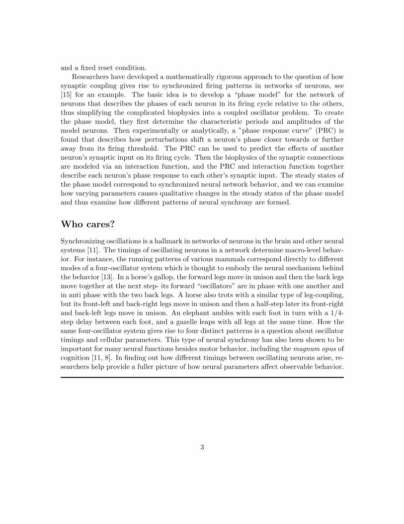
and a fixed reset condition.Researchers have developed a mathematically rigorous approach to the question of how
synaptic coupling gives rise to synchronized firing patterns in networks of neurons, see[15] for an example. The basic idea is to develop a “phase model” for the network ofneurons that describes the phases of each neuron in its firing cycle relative to the others,thus simplifying the complicated biophysics into a coupled oscillator problem. To createthe phase model, they first determine the characteristic periods and amplitudes of themodel neurons. Then experimentally or analytically, a ”phase response curve” (PRC) isfound that describes how perturbations shift a neuron’s phase closer towards or furtheraway from its firing threshold. The PRC can be used to predict the effects of anotherneuron’s synaptic input on its firing cycle. Then the biophysics of the synaptic connectionsare modeled via an interaction function, and the PRC and interaction function togetherdescribe each neuron’s phase response to each other’s synaptic input. The steady states ofthe phase model correspond to synchronized neural network behavior, and we can examinehow varying parameters causes qualitative changes in the steady states of the phase modeland thus examine how different patterns of neural synchrony are formed.
Who cares?
Synchronizing oscillations is a hallmark in networks of neurons in the brain and other neuralsystems [11]. The timings of oscillating neurons in a network determine macro-level behav-ior. For instance, the running patterns of various mammals correspond directly to differentmodes of a four-oscillator system which is thought to embody the neural mechanism behindthe behavior [13]. In a horse’s gallop, the forward legs move in unison and then the back legsmove together at the next step- its forward “oscillators” are in phase with one another andin anti phase with the two back legs. A horse also trots with a similar type of leg-coupling,but its front-left and back-right legs move in unison and then a half-step later its front-rightand back-left legs move in unison. An elephant ambles with each foot in turn with a 1/4-step delay between each foot, and a gazelle leaps with all legs at the same time. How thesame four-oscillator system gives rise to four distinct patterns is a question about oscillatortimings and cellular parameters. This type of neural synchrony has also been shown to beimportant for many neural functions besides motor behavior, including the magnum opus ofcognition [11, 8]. In finding out how different timings between oscillating neurons arise, re-searchers help provide a fuller picture of how neural parameters affect observable behavior.
3

Part I - Coupling in Morris-Lecar Neurons
2 Summary
The goal of this paper is to determine the timing of a Morris-Lecar model neuron’s os-cillations relative to the timing of periodic input. We create a phase model for a singleMorris-Lecar model neuron that describes how a coupled neuron moves about its naturalcycle in phase space as opposed to explicitly describing the oscillations of cellular parame-ters, much like how we describe the Earth’s motion about the sun by the calendar year asopposed to the Earth’s physical position about the sun. We will derive an ordinary differ-ential equation that describes the rate of change of the phase of the Morris-Lecar oscillatorin its periodic “limit cycle” relative to the phase of an external, periodic stimulus. Thefirst periodic input we will consider is just a simple injected sinusoidal current, but we willshow how to consider periodic input from another Morris-Lecar neuron. We will extendthe phase model to analyze the relative phases between any number of coupled neurons.
We will consider the Morris-Lecar model as our neural oscillator. This neuron’s oscil-lations are described by a system of ordinary differential equations (ODEs). To determinethe characteristic period and amplitude of the oscillator, we will use Euler’s method (onMATLAB) on the ODE system to iterate through the oscillator’s states and find the “limitcycle” of the system. The “limit cycle” is the periodic solution to the differential equations,or the cyclical pattern of states that the oscillator approaches as we run forwards in time.
We must also define “phase” on or near the limit cycle, so that we can be clear aboutwhat the phase model is even describing. Next, we derive the “phase response” functionZ(t) of the neuron: how many phases the neuron is shifted about its limit cycle aftera small perturbation to its steady oscillations. We use the “adjoint method” (see [12])to determine this. We then determine an interaction function G(X, t) that describes theeffects on the neuron by the periodic input. We will then combine the phase response andinteraction functions to create the phase model.
We will use a convolution integral (in accordance with Malkin Theorem for WeaklyCoupled Oscillators) of the interaction function with the PRC to combine the perturbationsthat the forcing field has on the neuron’s oscillations (the interaction function) with theresponse of the oscillator to external perturbations (the iPRC). This integral sums up thecell’s phase response to the ephaptic input and describes the phase evolution of the cell.This creates the phase model — an ODE that describes the oscillator’s phase in its cyclerelative to the phase of the stimulus. By analyzing the steady states of the phase model,we will describe the phase-locking behavior of the oscillator with the oscillating field. Thisgives us a clear picture of how the neuron’s oscillations are timed with the periodic input.
4
3 Technical Details
The Limit Cycle of the Morris-Lecar Model
The Morris-Lecar model describes the electrical dynamics of an oscillating neuron by
CdV
dt= −gCaMss(V )(V − VCa)− gKW (V − VK)− gL(V − VL) + Iapp (1)
dW
dt= φ(Wss(V )−W )/τ. (2)
Where
Mss(V ) =(
1 + tanh(V − V1
V2))/2 (3)
Wss(V ) =(
1 + tanh(V − V3
V4))/2. (4)
In each of these equations, all the parameters have been nondimensionalized. Equation(1) is a current balance equation for the cellular membrane potential. V is the cellularmembrane potential, and C is the membrane capacitance. (1) balances an applied currentIapp with three ionic currents: ICa - the excitatory Calcium ion current, IK - the recov-ery Potassium ion current, and IL - the equilibriating leakage current. The gi and Vi arethe conductances (or magnitudes) and equilibrium potentials of their respective ionic cur-rents. Mss(V ) is a probability distribution function describing the chance that a numberof Calcium ion channels will be open.
Equation (2) describes the recovery dynamics of the cell, and it dominates after thecell sends its signal. Specifically, W is the normalized Potassium ion conductance. φ and τare time constants for the opening and closing of the Potassium ion channels, and Wss(V )is a probability distribution function of open Potassium channels.
Equation (3), Mss(V ), is the probability distribution function of open Calcium ionchannels, with V1 as another voltage threshold and V2 as a voltage normalizer. Equation(4), Wss(V ), is the probability distribution function of open Potassium ion channels, withV3 as another voltage threshold and V4 as a voltage normalizer.
The solution to this system of ordinary differential equations for particular parametersets is a stable limit cycle. We use the parameter values from figures 8.6 and 8.7 in [10]because they yield a stable limit cycle solution to (1-2):P1 = C = 20; gCa = 4.4;VCa = 120; gK = 8;VK = −84; gL = 2;VL = −60;V1 = −1.2;V2 =18;V3 = 2;V4 = 30;φ = 0.04; τ = 0.8; .
By setting dV/dt = dW/dt = 0 (equations (1-2)), we can plot the nullclines to observethat the system has a limit cycle solution.
5
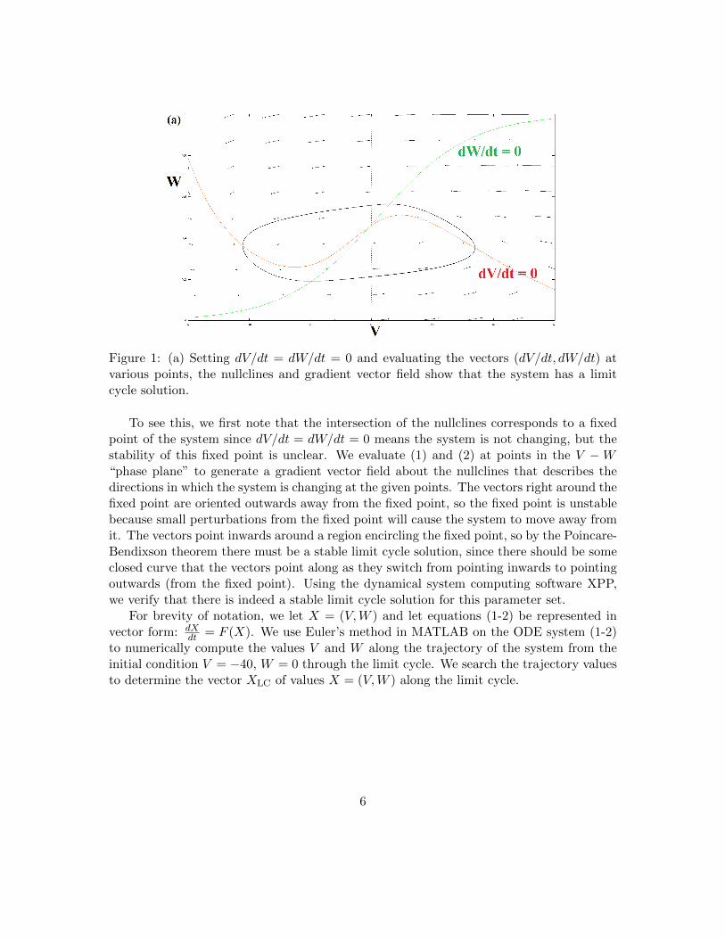
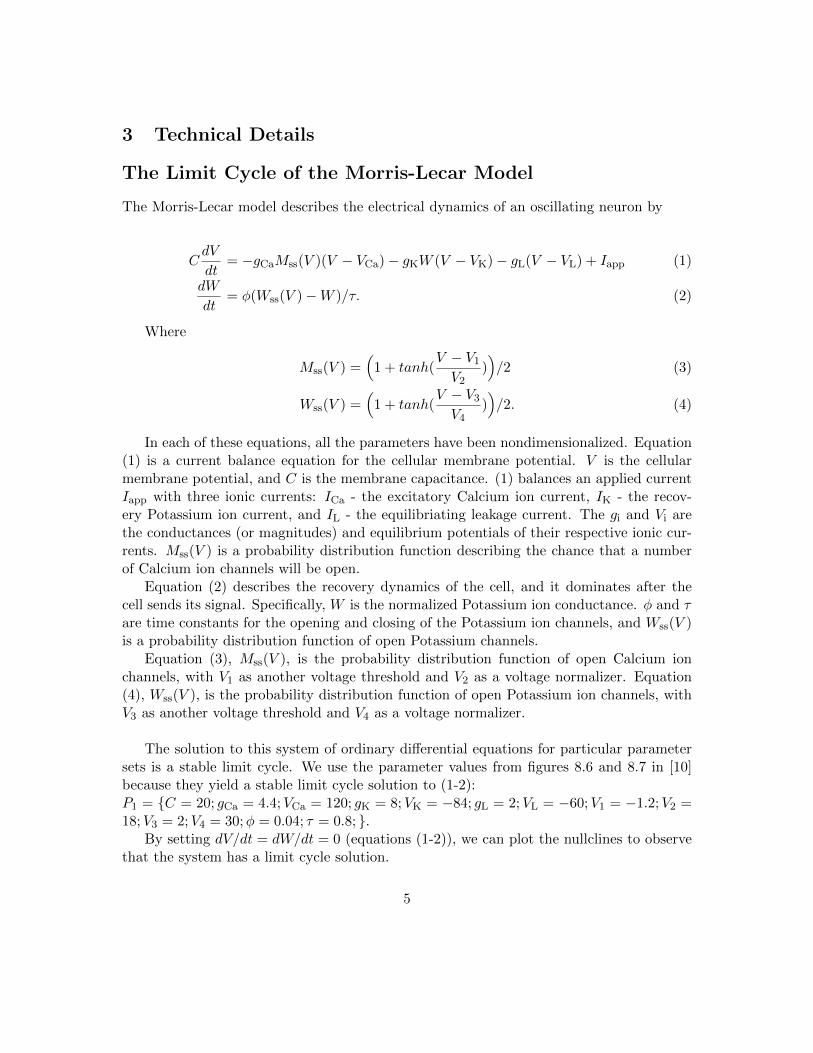
Figure 1: (a) Setting dV/dt = dW/dt = 0 and evaluating the vectors (dV/dt, dW/dt) atvarious points, the nullclines and gradient vector field show that the system has a limitcycle solution.
To see this, we first note that the intersection of the nullclines corresponds to a fixedpoint of the system since dV/dt = dW/dt = 0 means the system is not changing, but thestability of this fixed point is unclear. We evaluate (1) and (2) at points in the V −W“phase plane” to generate a gradient vector field about the nullclines that describes thedirections in which the system is changing at the given points. The vectors right around thefixed point are oriented outwards away from the fixed point, so the fixed point is unstablebecause small perturbations from the fixed point will cause the system to move away fromit. The vectors point inwards around a region encircling the fixed point, so by the Poincare-Bendixson theorem there must be a stable limit cycle solution, since there should be someclosed curve that the vectors point along as they switch from pointing inwards to pointingoutwards (from the fixed point). Using the dynamical system computing software XPP,we verify that there is indeed a stable limit cycle solution for this parameter set.
For brevity of notation, we let X = (V,W ) and let equations (1-2) be represented invector form: dX
dt = F (X). We use Euler’s method in MATLAB on the ODE system (1-2)to numerically compute the values V and W along the trajectory of the system from theinitial condition V = −40, W = 0 through the limit cycle. We search the trajectory valuesto determine the vector XLC of values X = (V,W ) along the limit cycle.
6

Figure 2: The trajectory of the system in V-W phase space according to (1-4) with initialcondition V = −40, W = 0. Computed numerically with Euler’s method in MATLABwith parameter set P1.
Figure 3: (L) The limit cycle solution to eqns. (1-2) for the cellular membrane potentialV . Computed numerically from Fig. 2 via a search routine. (R) The limit cycle solutionto eqns. (1-2) for the recovery variable W . Computed numerically from Fig. 2 via a searchroutine.
Defining Phase on and near the Limit Cycle
We want to clearly define the “phase” of the neuron on or near its limit cycle before wecan begin to define a neuron’s “phase response” to input or “phase-locking” in a pair ofneurons.
The limit cycle solution to equations (1-2) has some period T , so we define the phaseof the neuron along its limit cycle as
θ(t) = (t+ φ) mod T,
7
where the relative phase φ is a constant that is determined by where on the limit cycle theneuron begins. The position of the neuron in phase space, X(t) = XLC(θ(t)), is given in aone-to-one fashion by the phase, so each point on the limit cycle corresponds to a uniquephase θ = X−1
LC(X) = Φ(X).The limit cycle of the Morris-Lecar model neuron is stable, so every point in phase
space, if given as an initial condition to (1-2), will converge to the limit cycle as time goesto infinity. We can extend the domain of Φ(X) to points off of the limit cycle by definingthe “asymptotic phase” of a point as the phase of another point on the limit cycle whosetrajectory coincides with the approaching trajectory as time goes to infinity. This meansthat for points on the limit cycle, the asymptotic phase is the same as phase, but for pointsoff the limit cycle, we must match trajectories to a point on the limit cycle:
If X0 is a point on the limit cycle in phase space and Y0 is a point off the limit cycle,then Y0 has the same asymptotic phase as X0 if the solution to (1-2) with initial conditionY0 converges to the solution to (1-2) with initial condition X0 as time goes to infinity. Wesay that Φ(Y ) = Φ(X).
Figure 4: X0 is a point on the limit cycle in phase space and Y0 is a point off the limitcycle. Y0 has the same asymptotic phase as X0, i.e., Φ(Y ) = Φ(X).
The Infinitessimal Phase Response Curve
Here, we derive the “phase response” of a neuron’s oscillations to external input. Whenthe neuron receives input, it is bumped off its limit cycle to some other point in phasespace. But as we saw in the previous section, points off the limit cycle will converge tothe limit cycle as time goes to infinity, so we can look at the asymptotic phase of this newposition. The difference between this new asymptotic phase and the old asymptotic phase(or rather phase, since it was on the limit cycle) is called the “phase shift”. We quantifythese phase shifts in the infinitesimal phase response curve (iPRC). The iPRC is a periodic
8
function Z(t) that measures the shift in the asymptotic phase of the neuron in response toinfinitesimally small and instantaneous perturbations as a function of where in the limitcycle the neuron was when it was perturbed.
To derive the iPRC, note that the unit along the limit cycle of the oscillator is phase,so the rate of change of phase in time dθ
dt = 1. By differentiating θ = Φ(X), we get
dθ
dt= ∇XΦ(XLC(t)) · F (XLC(t)) = 1 (5)
where ∇XΦ is the gradient of Φ(X).The iPRC measures the oscillator’s phase shift in response to small perturbations, so
it is defined as the gradient of the phase map ∇XΦ(XLC(t)). To see this, suppose anoscillator on its limit cycle at X(t) = XLC(θ∗) with phase θ∗ = Φ(X(t)) is perturbed byεU , where ε << 1 is a magnitude and U is a unit vector in some direction in phase space.
Now the neuron is at the state XLC(θ∗) + εU with asymptotic phase θ = Φ(XLC(θ∗) +εU). Using Taylor series,
θ = Φ(XLC(θ∗) + εU) = Φ(XLC(θ∗)) +∇XΦ(XLC(θ∗))(εU) +O(ε2). (6)
Since ε << 1, we can ignore the remainder O(ε2). Then the phase shift of the oscillator is
∆φ(θ∗) = Φ(XLC(θ∗) + εU)− Φ(XLC(θ∗)) = ∇XΦ(XLC(θ∗)) · (εU).
So the phase shift is a function of the phase θ∗ at which it was perturbed. If we normalizeby the strength of the perturbation, we get that ∆φ(θ∗)/ε = ∇XΦ(XLC(θ∗) · U .
Thus the gradient of the asymptotic phase map along the limit cycle of the oscillatoris the iPRC. It quantifies the phase shift of the oscillator due to weak, brief perturbationsat any phase (or asymptotic phase) along the limit cycle.
In practice, however, this derivation of the iPRC yields little to no computational value.There is an alternate derivation, however, that gives us a straightforward numerical methodto compute the iPRC. This method is called the adjoint method, and requires that we firstintroduce the Theory of Weakly Coupled Oscillators.
The Theory of Weakly Coupled Oscillators
To show that the iPRC can be found via the adjoint method, we must introduce some moretheory. Fortunately, this theory also gives us a direct way to use the iPRC Z(t) and theinteraction function G(X, t) to derive the phase model of our system. It is the intermediatestep between the unperturbed neural behavior and the coupled neural behavior.
We consider our coupled Morris-Lecar model neuron. Let X = (V,W ) be the cellularmembrane potential and recovery variable for the uncoupled neuron, so that dX
dt = F (X)
9

is the uncoupled ODE system as in (1-2). Let G(X, t) be the interaction function for theneuron with the periodic input; we will derive this soon. Then the ODE for the coupledMorris-Lecar neuron’s oscillations is
dX
dt= F (X) + εG(X, t),
where ε << 1 since coupling is understood to be weak relative to the intrinsic dynamics ofthe neuron F (X).
We are interested in the difference between the phase of the neuron in its oscillations andthe phase of the oscillating forcing field, and how this “relative phase” difference changesover time as the neuron is periodically perturbed. We want to construct a phase model —an ODE that describes not the electrochemical states of the neuron but simply the relativephase of the neuron in its limit cycle. The phase model will describe how the neuron’s limitcycle timing is shifted as a result of the perturbations, and the steady states of the phasemodel will correspond to relative phase differences between the neuron and the periodicinput that do not change over time. Constant relative phase differences describe how theneuron’s oscillations are timed with respect to the timing of the stimulus.
The Malkin Theorem for Weakly Coupled Oscillators (see [5]) shows us how to derive aphase model for our system and yields a method of finding the infinitessimal phase responsecurve (iPRC).
Malkin Theorem for Weakly Coupled OscillatorsConsider a weakly coupled oscillator of the form
dX
dt= F (X) + εG(X, t),
that has an asymptotically stable T -periodic solution XLC when uncoupled (i.e., withinteraction function G(X, t) = 0).Let τ = εt be slow time and let φ(τ) ∈ [0, T ] be the phase shift away from the naturaloscillation XLC(t) (also in [0, T ]) that results from the coupling effects εG(X, t).Then, φ ∈ [0, T ] is a solution to
dφ
dτ=
1
T
∫ T
0Z(t+ φ) ·G(XLC(t+ φ), t)dt,
where Z(t) is the unique nontrivial T -periodic solution to the adjoint linear system
dZ
dt= −[DF (XLC(t))]TZ (7)
satisfying the normalization condition
Z(0) · F (XLC(0)) = 1, (8)
10

and where DF (XLC(t)) is the Jacobian of partial derivatives of the vector function F (X)evaluated along the limit cycle XLC(t).
We have already computed the limit cycle XLC in the previous subsection, but we’restill missing Z(t) and G(X). We will derive the T -periodic function Z(t), which coincideswith the infinitessimal phase response curve (the iPRC). We will prove that Z(t) is exactlythe iPRC of the neuron by showing that ∇XΦ(XLC(t)) satisfies the adjoint equation (7)and the normalization condition (8) in Malkin Theorem.
Theorem The iPRC ∇XΦ(XLC(t)) satisfies
d
dt∇XΦ(XLC(t)) = −[DF (XLC(t))]T∇XΦ(XLC(t)) (9)
and
∇XΦ(XLC(0)) · F (XLC(0)) = 1. (10)
Proof. Consider two solutions to the system (1-2):X(t) = XLC(t + φ) and Y (t) = XLC(t + φ) + p(t), where p(t) is the trajectory backonto the limit cycle from a small perturbation p(0) << 1. X(t) starts on the limit cycleat X(0) = XLC(φ), while Y (t) starts just off the limit cycle at Y (0) = XLC(φ) + p(0).The initial perturbation p(0) is small and the limit cycle is stable, so Y (t) approachesXLC(t+ φ2), where φ2 6= φ.
Thus p(t) remains small (i.e., |p| << 1) and since Y (t) remains close to the limit cycle,
dXLC(t)
dt+dp
dt=dY
dt= F (Y (t))
F (XLC(t)) +dp
dt= F (XLC(t)+p(t))
and by Taylor Series, we can expand F (XLC(t) + p(t)) so that
F (XLC(t)) +dp
dt= F (XLC(t))+DF (XLC(t)) · p(t) +O(|p|2),
where DF (XLC(t)) is the Jacobian matrix of partial derivatives of the vector functionF (X) evaluated along the limit cycle XLC(t). Since |p| << 1, we can ignore the O(|p|2)term and thus p(t) satisfies dp
dt = DF (XLC(t+ φ)) · p(t).The phase difference between the two solutions is
∆φ = Φ(XLC(t+ φ) + p(t))− Φ(XLC(t+ φ)) = ∇XΦ(XLC(t+ φ)) · p(t) +O(|p|2), (11)
where the last equality holds by our derivation for the iPRC.
11

The two solutions continue as time goes to infinity without any further perturbations,so the phase difference has no impetus to change. The asymptotic phases of these solutionsevolve in time as the solutions travel about the limit cycle, but the phase difference betweenthem, ∆φ, remains constant. Taking the derivative of (11),
0 =d
dt
(∇XΦ(XLC(t+ φ)) · p(t)
)=
d
dt
(∇XΦ(XLC(t+ φ))
)· p(t) +∇XΦ(XLC(t+ φ) · dp
dt
=( ddt
(∇XΦ(XLC(t+ φ))
)+DF (XLC(t+ φ))T (∇XΦ(XLC(t+ φ)))
)· p(t)
This holds for any arbitrarily small perturbation p(t) in any direction in phase space,so we have that
d
dt
(∇XΦ(XLC(t+ φ))
)= −DF (XLC(t+ φ))T (∇XΦ(XLC(t+ φ))). (12)
Hence ∇XΦ(XLC(t)) satisfies the adjoint equation (9). The normalization condition (10)is satisfied by the definition of the phase map since dθ
dt = ∇XΦ(XLC(t)) ·X ′LC(t) = 1.
To compute the iPRC Z(t), we note that since equation (7) is the adjoint system tothe isolated model neuron linearized around its limit cycle, it has the opposite stabilityof the original system. Thus we integrate equation (7) backwards in time using Euler’smethod to get the unstable periodic solution. We then normalize the periodic solution bycomputing Z(t) · F (XLC(t)) for every t ∈ [0, T ] and dividing Z(t) by the average value.
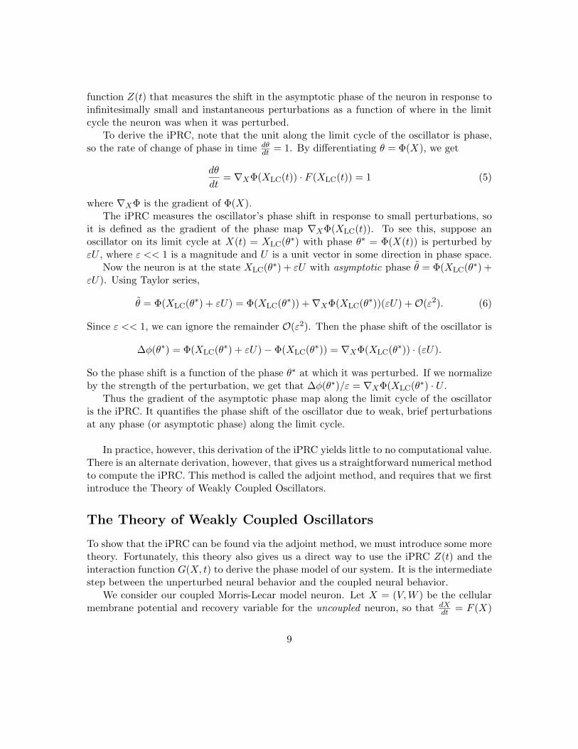
The iPRC Z(t) measures the response of a Morris-Lecar neuron’s oscillations to weakperturbations. It has two components: a voltage response in V , and a recovery variableresponse in W . Each response curve quantifies the amount by which the respective variablewill be shifted (the y-axis) following an infinitessimally small, instantaneous perturbationat a particular timing in the limit cycle (the x-axis).
12
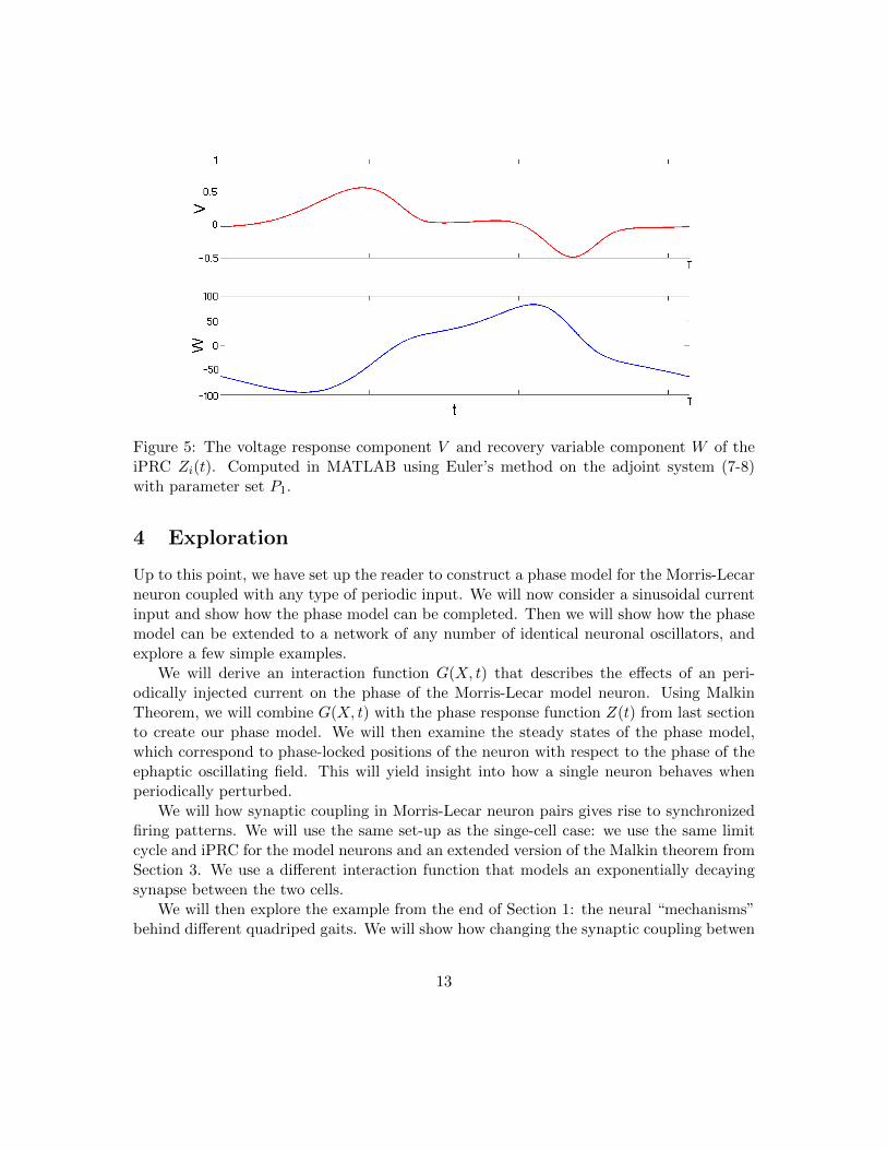
Figure 5: The voltage response component V and recovery variable component W of theiPRC Zi(t). Computed in MATLAB using Euler’s method on the adjoint system (7-8)with parameter set P1.
4 Exploration
Up to this point, we have set up the reader to construct a phase model for the Morris-Lecarneuron coupled with any type of periodic input. We will now consider a sinusoidal currentinput and show how the phase model can be completed. Then we will show how the phasemodel can be extended to a network of any number of identical neuronal oscillators, andexplore a few simple examples.
We will derive an interaction function G(X, t) that describes the effects of an peri-odically injected current on the phase of the Morris-Lecar model neuron. Using MalkinTheorem, we will combine G(X, t) with the phase response function Z(t) from last sectionto create our phase model. We will then examine the steady states of the phase model,which correspond to phase-locked positions of the neuron with respect to the phase of theephaptic oscillating field. This will yield insight into how a single neuron behaves whenperiodically perturbed.
We will how synaptic coupling in Morris-Lecar neuron pairs gives rise to synchronizedfiring patterns. We will use the same set-up as the singe-cell case: we use the same limitcycle and iPRC for the model neurons and an extended version of the Malkin theorem fromSection 3. We use a different interaction function that models an exponentially decayingsynapse between the two cells.
We will then explore the example from the end of Section 1: the neural “mechanisms”behind different quadriped gaits. We will show how changing the synaptic coupling betwen
13

four Morris-Lecar neurons gives rise to the many different four-oscillator patterns.
The Single Cell with a Sinusoidal Current Input
Here we derive the interaction function G(X, t) that describes the sinusoidal input to theMorris-Lecar model neuron and show how the cell phase-locks with the current.
Figure 6: The single cell with sinusoidal input.
The sinusoidal current I(t) has the same period as the neuron, and it is given by
I(t) = A · sin(2πt
T), (13)
where A is the amplitude of the current and T is the period of the Morris-Lecar neuron’slimit cycle.
Because the current is injected straight across the cellular membrane, the effect on thecell is exactly the sinusoidal current. See [1] for a further exploration of sinusoidal currentinjections. Thus G(X, t) = I(t).
We now finally have all the pieces to create the phase model for the Morris-Lecar modelneuron with a sinusoidal current input. We have the limit cycle of the neuron XLC(t), thephase response function Z(t), and the interaction function G(X, t). Referring back toMalkin Theorem for Weakly Coupled Oscillators, we have that the phase shifts φ awayfrom the natural oscillations XLC(t) solve
dφ
dτ=
1
T
∫ T
0Z(t) ·G(XLC(t), t− φ)dt =
1
T
∫ T
0Z(t) · I(t− φ)dt, (14)
We numerically compute the values of equation (14) in [0, T ] using a MATLAB routine.We then search this solution for zeroes, which correspond to fixed phase differences of thesystem, and align our limit cycle XLC with the periodic input eqn. (13) at the stable phasedifference to illustrate the natural timing of the system.
The Interaction Function for Synaptic Interactions
Now we want to use our thoroughly examined techniques to explore how phase-locking oc-curs between any number of Morris-Lecar neurons. We will use a non-summing, exponentially-decaying synapse for the connections between neurons, as in [6]. This type of synaptic input
14
is modeled via
S(t) = αe−t/τ , (15)
where α is the strength of the synaptic coupling, and τ is the synaptic decay rate. Wetake α > 0 to indicate an excitatory synapse and α < 0 to indicate an inhibitory synapse.Since the magnitude of α will not affect the phase-locking results, we take |α| = 1, and wealso take τ = 100 as in [6]. We take our interaction function for effect of input from thejth neuron onto the ith neuron to be
G(Xi, Xj , t) = S(t− ψi,j),
where ψi,j = φj −φi is the relative phase difference between the phase φi of the ith neuron
in its limit cycle XiLC and the phase φj of the jth neuron in its limit cycle Xj
LC.
An Extended Version of Malkin Theorem
We must extend Malkin Theorem from Section 3 to analyze a network of n coupled, iden-tical Morris-Lecar neurons. See [5] for a full derivation.
Malkin Theorem for Weakly Coupled OscillatorsConsider a system of weakly coupled oscillators of the form
dXi
dt= F (Xi) + εG(Xi, Xj , t), i = 1, . . . , n,
where each ODE has an asymptotically stable T -periodic solution XiLC when uncoupled
(i.e., with interaction function G(Xi, Xj , t) = 0).Let τ = εt be slow time and let φi(τ) ∈ [0, T ] be the phase shift of the ith neuron awayfrom its limit cycle oscillations Xi
LC(t) (also in [0, T ]) that results from the coupling effectsεG(Xi, Xj , t).Then, φi ∈ [0, T ] (i = 1, . . . , n) is a solution to
dφidτ
=1
T
∫ T
0Z(t) ·
n∑j=1
G(XiLC(t), Xj
LC(t+ φj − φi), t)dt,
where Z(t) is the iPRC for the identical cells.
The Two-Cell Phase Model
Here we consider a pair of Morris-Lecar model neurons connected together via exponen-tially decaying synapses. Inhibitory synapses (negative α in eqn.(15)) will yield antiphasesynchrony, while excitatory synapses (positive α) will yield in-phase synchrony.
15

Figure 7: The two-cell network.
We are interested in the difference between the phase of the first neuron in its oscilla-tions and the phase of the second neuron in its oscillations, and how this “relative phase”difference changes over time as the neuron perturb one another. We want to construct aphase model — a pair of ODEs that describe not the electrochemical states of each neuronbut simply the relative phases of each neuron in its limit cycle. The phase model will de-scribe how each neuron’s limit cycle timing is shifted as a result of the perturbations, andthe steady states of the phase model will correspond to relative phase differences betweenthe two neurons that do not change over time. Constant relative phase differences describehow the first neuron’s oscillations are timed with respect to the oscillations of the secondneuron.
The Malkin Theorem for Weakly Coupled Oscillators yields the phase model for ourtwo-cell system.
dφidτ
=1
T
∫ T
0Z(t) · αS(t+ φj − φi)dt, i, j = 1 , 2,
We numerically compute the values of the two ODEs in [0, T ] using a MATLAB routine.We then find the evolution of the relative phase difference
dψ
dτ=dφ2
dτ− dφ1
dτ. (16)
We then search eqn. (16) for zeroes, which correspond to fixed phase differences of thesystem, and align the first limit cycle, X1
LC, with the second limit cycle, X2LC, at the stable
phase difference to illustrate the natural timing of the system.
The Four-Cell Phase Model
Here we consider a set of four Morris-Lecar neurons connected together via exponentiallydecaying synapses.
16

Figure 8: The four-cell network.
The Malkin Theorem for Weakly Coupled Oscillators yields the phase model for ourfour-cell system.
dφ1
dτ=
1
T
∫ T
0Z(t) ·
[α1,2S(t+ φ2 − φ1) + α1,3S(t+ φ3 − φ1) + α1,4S(t+ φ4 − φ1)
]dt
dφ2
dτ=
1
T
∫ T
0Z(t) ·
[α1,2S(t+ φ1 − φ2) + α2,3S(t+ φ3 − φ2) + α2,4S(t+ φ4 − φ2)
]dt
dφ3
dτ=
1
T
∫ T
0Z(t) ·
[α1,3S(t+ φ1 − φ3) + α2,3S(t+ φ2 − φ3) + α3,4S(t+ φ4 − φ3)
]dt
dφ4
dτ=
1
T
∫ T
0Z(t) ·
[α1,4S(t+ φ1 − φ4) + α2,4S(t+ φ2 − φ4) + α3,4S(t+ φ3 − φ4)
]dt,
The intrepid reader who has made it this far is now probably wondering to themselfwhat sort of foul sorcery must be summoned to analyze this beast of a model. We canexamine the symmetry of the network to simplify the problem and find the phase-lockeddifferences between these four cells.
If we take the four cells and split them into two pairs, we can connect each pair withexcitatory synapses to induce in-phase synchrony between the two, and then we can connectthe two pairs together with inhibitory synapses to induce antiphase synchrony. Setting allαi,j equal in magnitude, we let αi,j > 0 for excitatorily coupled pairs i, j and αi,j < 0 for
inhibitorily coupled pairs i, j, the system of relative phase differencesdψi,j
dτ =dφjdτ −
dφidτ
simplifies.As an example, considered the network where cells 1 and 2 are paired together with
excitatory synapses, cells 3 and 4 are paired together with identical excitatory synapses,and the two sets of pairs are coupled together with identical inhibitory synapses between
17

cells 1 and 4 and between cells 2 and 3. Then the relative phase differences simplify:
dψ1,2
dτ=dφ2
dτ− dφ1
dτ=
1
T
∫ T
0Z(t) ·
[α1,2(S(t+ φ1 − φ2)− S(t+ φ2 − φ1))
+ α2,3S(t+ φ3 − φ2)− α1,4S(t+ φ4 − φ1)]dt
=⇒ dψ1,2
dτ=
1
T
∫ T
0Z(t) · α1,2
[S(t+ φ1 − φ2)− S(t+ φ2 − φ1)
]dt,
since α2,3 = α1,4 and the convolutions with S will be the same because of symmetricalbehavior.
dψ1,4
dτ=dφ4
dτ− dφ1
dτ=
1
T
∫ T
0Z(t) ·
[α1,4(S(t+ φ1 − φ4)− S(t+ φ4 − φ1))
+ α3,4S(t+ φ3 − φ4)− α1,2S(t+ φ2 − φ1)]dt
=⇒ dψ1,4
dτ=
1
T
∫ T
0Z(t) · α1,4
[S(t+ φ1 − φ4)− S(t+ φ4 − φ1)
]dt,
since α3,4 = α1,2 and the convolutions with S will be the same because of symmetricalbehavior. Similarly,
dψ1,3
dτ=dφ3
dτ− dφ1
dτ=
1
T
∫ T
0Z(t) · α1,3
[S(t+ φ1 − φ3)− S(t+ φ3 − φ1)
]dt.
Each of these ODE’s is the same as eqn. (16), albeit with a different sign for α. Thus cells1 and 2 are indeed coupled in in-phase synchrony, cells 1 and 4 are coupled in antiphase,cells 1 and 3 are coupled in antiphase. Thus we can infer that cells 3 and 4 are coupledin-phase, that cells 2 and 3 are coupled in antiphase, and that cells 2 and 4 are coupled inantiphase.
Varying the pairings of the four cells, we can obtain any similar pairing pattern — wherewe have two pairs each in in-phase synchrony but offset from one another. By changingthe coupling between the two sets of pairs to excitatory synapses, we will obtain in-phasesynchrony between the pairs.
There is one more behavior we can still obtain: a phase difference of 1/4 between eachcell in a ring. That is to say, for example, that if cell 1 is at phase 0, then cell 2 is at phase1/4, cell 3 is at phase 1/2, and cell 4 is at phase 3/4. This can be obtained by settingall the α equal, and whether the synapses are inhibitory or excitatory (i.e., whether α ispositive or negative), we will be able to obtain this phase-locked state.
18
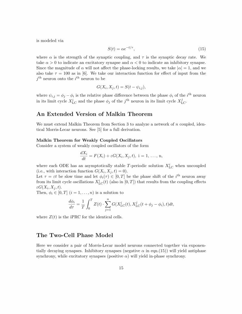
Considerdψ1,2
dτ with αi,j = α for all i, j and with φ1 = 0, φ2 = 1/4, φ3 = 1/2, φ4 = 3/4:
dψ1,2
dτ=dφ2
dτ− dφ1
dτ=
1
T
∫ T
0Z(t) · α
[S(t+ φ1 − φ2)− S(t+ φ2 − φ1) + S(t+ φ3 − φ2)− S(t+ φ4 − φ1)
]dt
dψ1,2
dτ=
1
T
∫ T
0Z(t) · α
[S(t− 1/4)− S(t+ 1/4) + S(t+ 1/4)− S(t+ 3/4)
]dt
dψ1,2
dτ= 0,
where the last equality holds because S(t− 1/4) = S(t+ 3/4) because −3/4 is the same as+1/4 when phase is in [0, 1]. Thus the pattern of 1/4 phase differences between cells in aring is a possible phase-locked position for a set of 4 Morris-Lecar neurons.
5 Results
The Single Cell with a Sinusoidal Current Input
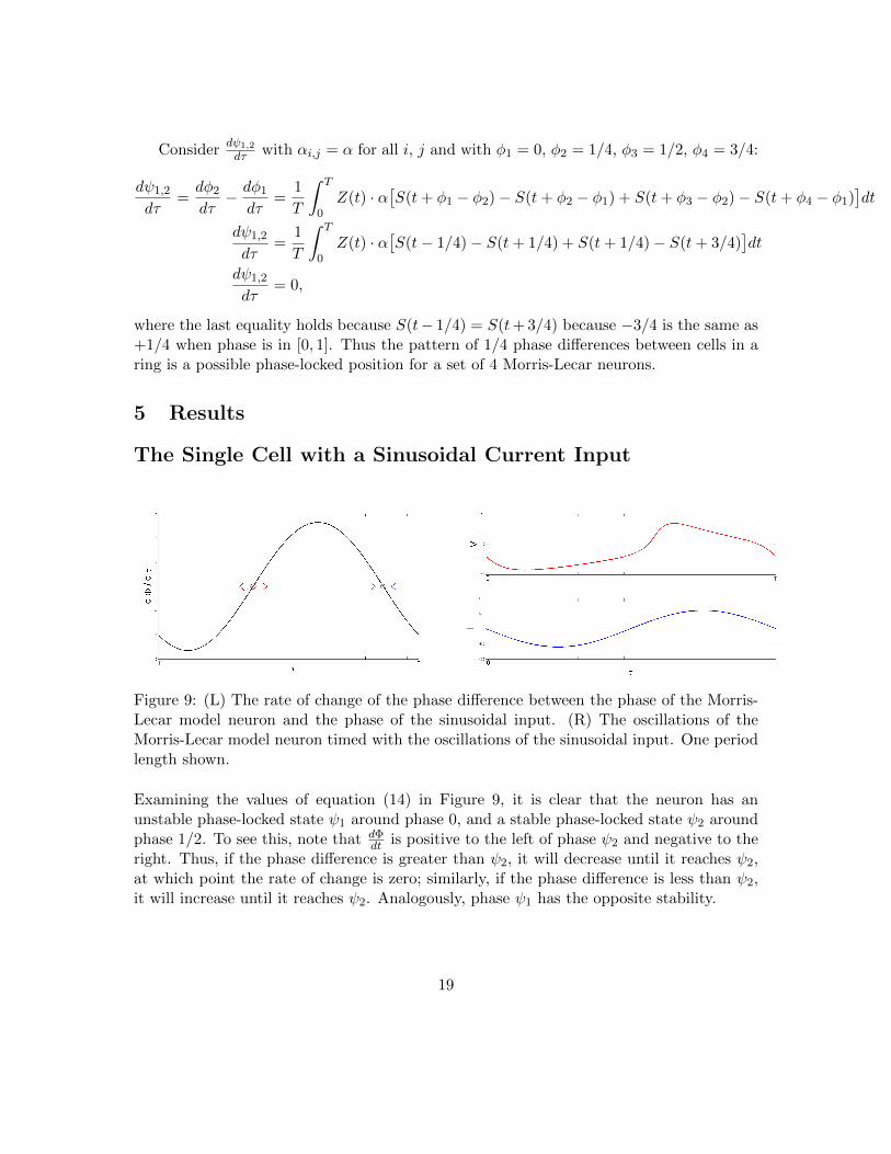
Figure 9: (L) The rate of change of the phase difference between the phase of the Morris-Lecar model neuron and the phase of the sinusoidal input. (R) The oscillations of theMorris-Lecar model neuron timed with the oscillations of the sinusoidal input. One periodlength shown.
Examining the values of equation (14) in Figure 9, it is clear that the neuron has anunstable phase-locked state ψ1 around phase 0, and a stable phase-locked state ψ2 aroundphase 1/2. To see this, note that dΦ
dt is positive to the left of phase ψ2 and negative to theright. Thus, if the phase difference is greater than ψ2, it will decrease until it reaches ψ2,at which point the rate of change is zero; similarly, if the phase difference is less than ψ2,it will increase until it reaches ψ2. Analogously, phase ψ1 has the opposite stability.
19

The pair of Morris-Lecar neurons with synaptic connections
Case 1: Inhibitory Coupling (α < 0).
Figure 10: (L) The rate of change of the phase difference between the phases of the twoMorris-Lecar model neurons inhibitorily coupled. (R) The oscillations of the Morris-Lecarmodel neuron timed with the oscillations of the second. One period length shown.
Examining the values of equation (14) in Figure 10, it is clear that the neuron has anunstable phase-locked state ψ1 around phase 0, and a stable phase-locked state ψ2 aroundphase 1/2. To see this, note that dΦ
dt is positive to the left of phase ψ2 and negative to theright. Thus, if the phase difference is greater than ψ2, it will decrease until it reaches ψ2,at which point the rate of change is zero; similarly, if the phase difference is less than ψ2,it will increase until it reaches ψ2. Analogously, phase ψ1 has the opposite stability.
Case 2: Excitatory Coupling (α > 0).
Figure 11: (L) The rate of change of the phase difference between the phases of the twoMorris-Lecar model neurons excitatorily coupled. (R) The oscillations of the Morris-Lecarmodel neuron timed with the oscillations of the second. One period length shown.
Examining the values of equation (14) in Figure 9, it is clear that the neuron has a
20
stable phase-locked state ψ1 around phase 0, and a stable phase-locked state ψ2 aroundphase 1/2. To see this, note that dΦ
dt is positive to the left of phase ψ1 and negative to theright. Thus, if the phase difference is greater than ψ1, it will decrease until it reaches ψ1,at which point the rate of change is zero; similarly, if the phase difference is less than ψ1,it will increase until it reaches ψ1. Analogously, phase ψ2 has the opposite stability.
The Four Cell System
Case 1: Inner-Pair Synchrony, Intra-Pair Antiphase.
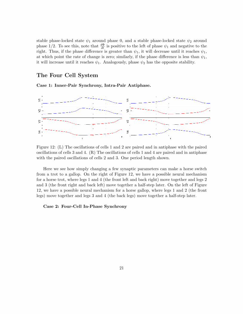
Figure 12: (L) The oscillations of cells 1 and 2 are paired and in antiphase with the pairedoscillations of cells 3 and 4. (R) The oscillations of cells 1 and 4 are paired and in antiphasewith the paired oscillations of cells 2 and 3. One period length shown.
Here we see how simply changing a few synaptic parameters can make a horse switchfrom a trot to a gallop. On the right of Figure 12, we have a possible neural mechanismfor a horse trot, where legs 1 and 4 (the front left and back right) move together and legs 2and 3 (the front right and back left) move together a half-step later. On the left of Figure12, we have a possible neural mechanism for a horse gallop, where legs 1 and 2 (the frontlegs) move together and legs 3 and 4 (the back legs) move together a half-step later.
Case 2: Four-Cell In-Phase Synchrony
21
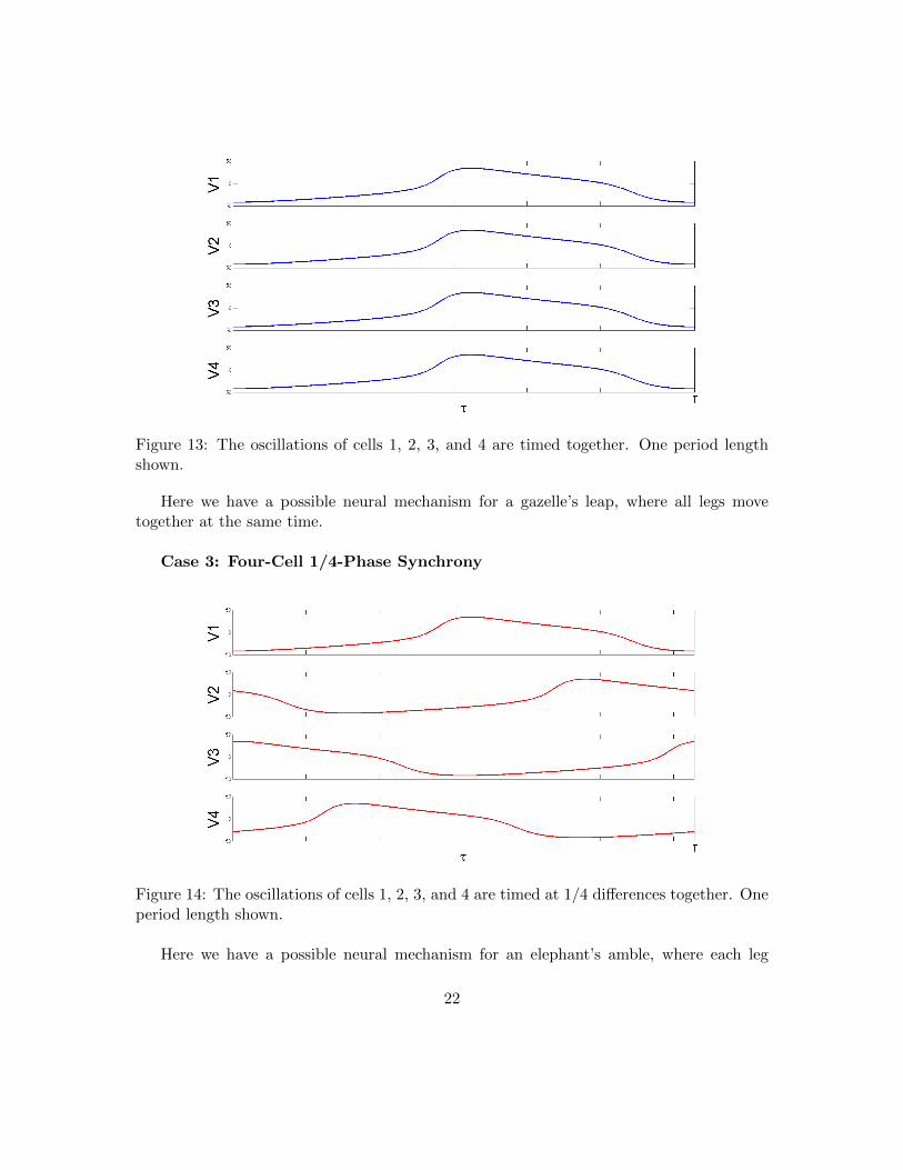
Figure 13: The oscillations of cells 1, 2, 3, and 4 are timed together. One period lengthshown.
Here we have a possible neural mechanism for a gazelle’s leap, where all legs movetogether at the same time.
Case 3: Four-Cell 1/4-Phase Synchrony
Figure 14: The oscillations of cells 1, 2, 3, and 4 are timed at 1/4 differences together. Oneperiod length shown.
Here we have a possible neural mechanism for an elephant’s amble, where each leg
22

moves in turn with a 1/4-step between each movement. Thus the four-cell neural oscillatorsystem is capable of each of the synchronizations mentioned in Section 1, and which patternthe system is in depends entirely on the structure and connectivity of the four neurons.
6 Closing Remarks
The possibilities for modeling neural systems are endless now that we have been caughtup to speed on how to derive the phase model for the Morris-Lecar neurons. In fact,one can extend our derivation to any other neural model, or even any sort of modelwith a periodic solution. One can vary the connections between neurons, the structureof the neural network, and even the neural parameters themselves to study almost anyobservable behavior. Varying the parameters of individual neurons throughout the sys-tem allows one to study the effects of heterogeneity on neural behavior, while varyingthe synaptic connection parameters between neurons throughout the system is anotherway to study these same effects. One can study even further the effects of differing in-put to single neurons, and still more work can be done to study alternative connectionmechanisms such as ephaptic coupling in neural networks. In Part II, we will explore theeffects of adding neural delays to the individual neuron and to the system of neurons.
23
Part II - Phase Response Propertiesand Phase-Locking in Neural Systems
with Delayed Negative-Feedback
7 Introduction
Synchronous activity is a hallmark in networks of neurons in the brain and other neuralsystems. This synchrony is often associated with oscillatory behavior[11] and has beenshown to be important for a multitude of neural functions, including motor behavior andcognition [11, 8]. Coordinated oscillations arise from the combination of intrinsic propertiesof neurons, synaptic coupling between neurons, and indirect or direct synaptic feedbackto a neuron. Synchronous activity (sometimes with nonzero phase lag) occurs despite theinherent delays in synaptic communication pathways between neurons [8]. These delaysarise from conduction delays in dendrites and axons, synaptic kinetics, and polysynapticpathways [9, 7, 3].
Here we use an idealized model to examine how synaptic delays in feedback pathwaysshape the properties of the oscillatory activity, including the period and the response toexternal input, and also how delays in synaptic coupling between cells affect synchroniza-tion. The model neuron we examine is a leaky integrate-and-fire (LIF) neuron that hasan applied constant current and a self-inhibiting synapse with a delay, which we call theDelayed Self-Inhibition (DSI) Cell. This simple model captures the qualitative behavior ofsimple neuron populations with delayed negative-feedback mechanisms.
We first determine how the DSI cell’s characteristic period depends on cellular andsynaptic feedback parameters. We then quantify the cell’s phase response to perturbationsat various phases in its cycle, defining the infinitessimal phase response curve (iPRC). TheiPRC is then used along with the theory of weak coupling [12] to analyze interactionsbetween a pair of DSI cells. We couple two DSI cells together via inhibitory synapses withdelays, and model the evolution of the phase difference between the two cells. We thenexamine the effect of varying the synaptic delay between the two cells and describe thebifurcations that occur in the phase-locking behavior of the two-cell system.
8 The Delayed Self-Inhibitory (DSI) Cell
The standard Leaky Integrate-and-Fire (LIF) model idealizes the electrical dynamics ofa neuron by including only a leakage current and a bias current I in the subthresholddynamics and reducing the action potential (or spike) to a single spike-reset condition.With all variables and parameters nondimensionalized, the cell’s membrane potential V
24
evolves according to the differential equation
dV
dt= −V + I. (17)
When the membrane potential hits the firing threshold at V = 1, the cell ”fires” a spikeand the membrane potential is reset to V = 0, i.e.,
V (t−) = 1→ V (t+) = 0. (18)
Given a constant bias current I and an initial condition V (0) = 0, the membrane potentialof the cell evolves according to
V (t) = I(1− e−t). (19)
If I > 1, the cell will reach the threshold V = 1, ”spike”, reset to V = 0, evolve againaccording to equation (19), and repeat this process with a characteristic oscillatory period(see Figure 16(a)). The period ∆T ∗ can be determined by setting V (∆T ∗) = 1 in equation(19) and solving for ∆T ∗, yielding
∆T ∗ = ln( I
I − 1
). (20)
Notice that the period monotonically decreases as the bias current I is increased.
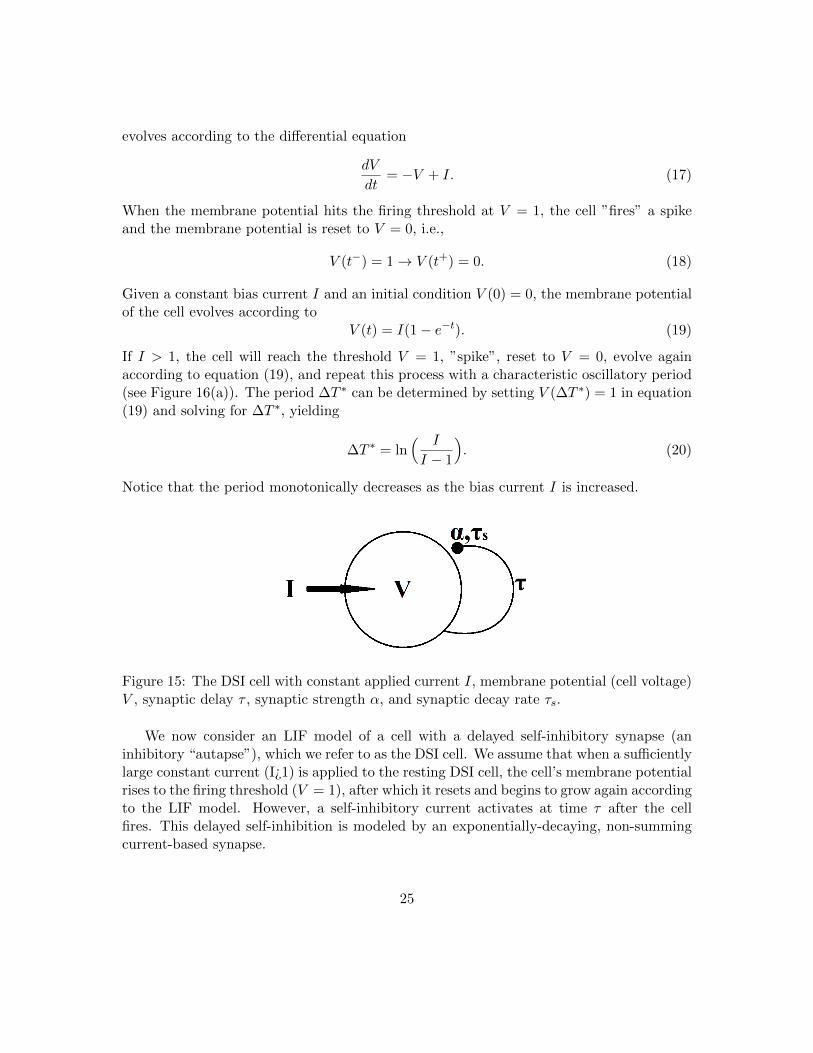
Figure 15: The DSI cell with constant applied current I, membrane potential (cell voltage)V , synaptic delay τ , synaptic strength α, and synaptic decay rate τs.
We now consider an LIF model of a cell with a delayed self-inhibitory synapse (aninhibitory “autapse”), which we refer to as the DSI cell. We assume that when a sufficientlylarge constant current (I¿1) is applied to the resting DSI cell, the cell’s membrane potentialrises to the firing threshold (V = 1), after which it resets and begins to grow again accordingto the LIF model. However, a self-inhibitory current activates at time τ after the cellfires. This delayed self-inhibition is modeled by an exponentially-decaying, non-summingcurrent-based synapse.
25

Figure 16: (a) The evolution of the LIF cell’s membrane potential V (t) for I = 1.1. (b) Theevolution of the DSI cell’s membrane potential V (t) and (c) synaptic waveform S(t − τ)for I = 1.1, α = .5, τ = 1.1, τs = 2.
The dynamics of the DSI cell are described by
dV
dt= −V + I − αS(t− τ), (21)
dS
dt=−Sτs, (22)
V (t−) = 1→ S(t+) = 1.
V (t+) = 0
In equation (21), αS(t− τ) is the delayed synaptic current where α is the nondimensionalsynaptic strength, S(t) is the time-dependent synaptic waveform, and τ is the fixed delay.In equation (22), τs is the decay rate of the exponential synapse.
Figure 16(b) illustrates the suppressing effect of the synaptic self-inhibition on the DSIcell’s oscillatory activity as described in equations (21 -22). The peak of the synapticcurrent corresponds to the activation of the inhibitory autapse and occurs τ time afterthe spike of the DSI membrane potential (see Figure 16(c). The inhibition suppresses thecell’s voltage and thus lengthens the inter-spike intervals compared to the standard LIFcell (compare Figure 16(a) and (b)). In section II, we show how to compute the periodsemi-analytically.
9 Evolution of the Inter-Spike Interval and the Character-istic Period of the DSI Cell
In order to examine the phase-locking and phase-response properties of the DSI cell, wemust first determine the period of the cell’s oscillatory activity and the period’s dependence
26

on parameter values. This involves a significantly more extensive derivation than thederivation for the period of the LIF model in equation (20). Calculating the period ofthe DSI cell involves finding a piecewise solution of equations (21-22) for the successiveinterspike intervals and then combining these solutions to define an interspike-interval(ISI) map. The fixed point of the ISI map corresponds to the period of the DSI cell.
To construct the ISI map, first suppose that the cell spikes and is reset to V = 0 attime t = Tk−1. The inhibitory autapse activates at time t = Tk−1 + τ (point A in Figure17). We define the cell’s voltage at the onset of inhibiton to be Vk = V (Tk−1 + τ). Vevolves according to equation (21) between time Tk−1 + τ and the next firing time Tk, withthe synaptic current decaying exponentially according to equation (22). Therefore we canintegrate equation (21) from Tk−1 + τ to Tk (point A to point B) to obtain
V (Tk)eTk − VkeTk−1+τ =
I(eTk − eTk−1+τ )− α∫ Tk
Tk−1+τetS(t− τ) dt. (23)
Figure 17: The firing times Ti (blue) and the voltage values Vi = V (Ti−1 + τ) (red) at theinhibition-activation timings Ti−1 + τ (black).
To find the firing time Tk and thus the kth inter-spike interval ∆Tk = Tk − Tk−1, we set
27

V (T−k ) = 1 and solve equation (23) for Vk
Vk = e∆Tk−τ − I(e∆Tk−τ − 1)
+ ατs
τs − 1
(e
(∆Tk−τ)(τs−1)
τs − 1)
= F (∆Tk). (24)
Note that equation (24) gives the ISI ∆Tk implicitly in terms of Vk.To complete a full cycle of the oscillatory activity of the DSI cell, we must find the cell’s
voltage when the autapse is next activated, i.e., Vk+1 = V (Tk + τ) (point A’ in Figure 17).We integrate equation (21) from Tk to Tk + τ (point B to point A’) with initial conditionV (T+
k ) = 0 to obtain
Vk+1 = I(1− e−τ )− ατsτs − 1
e−(∆Tk−τ)
τs
(e
−ττs − e−τ
)= G(∆Tk). (25)
Equation (25) gives the voltage at the time at which the delayed inhibition activates,Vk+1, in terms of the preceding ISI ∆Tk. By equating equation (24) in the form Vk+1 =F (∆Tk+1) with equation (25), we create a finite-difference equation for successive ISIs,which we call the ISI map
F (∆Tk+1) = G(∆Tk). (26)
This map takes the kth inter-spike interval duration ∆Tk as input and outputs the durationof the (k + 1)th inter-spike interval Tk+1. It captures the essential dynamics of the repet-itively firing DSI cell subject to a contant bias current, and it can be iterated to find theevolution of the inter-spike intervals ∆Tk. The fixed point F (∆T ∗) = G(∆T ∗) correspondsto the characteristic period of the DSI cell.
28
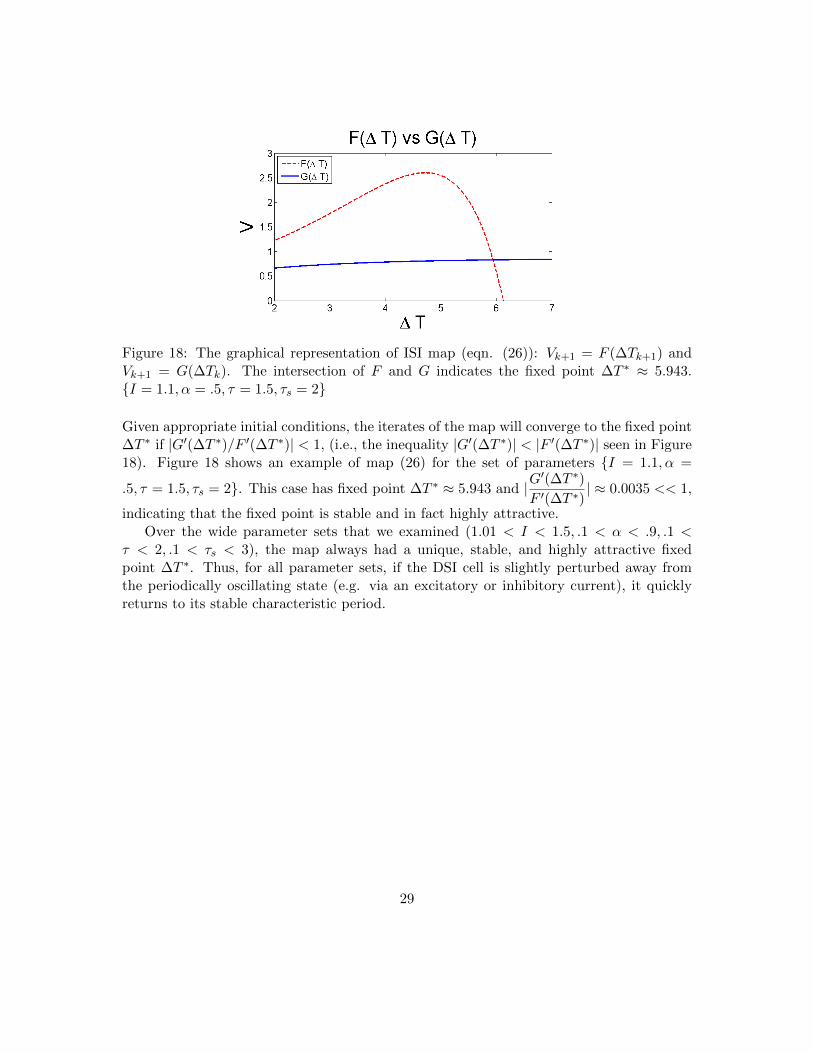
Figure 18: The graphical representation of ISI map (eqn. (26)): Vk+1 = F (∆Tk+1) andVk+1 = G(∆Tk). The intersection of F and G indicates the fixed point ∆T ∗ ≈ 5.943.I = 1.1, α = .5, τ = 1.5, τs = 2
Given appropriate initial conditions, the iterates of the map will converge to the fixed point∆T ∗ if |G′(∆T ∗)/F ′(∆T ∗)| < 1, (i.e., the inequality |G′(∆T ∗)| < |F ′(∆T ∗)| seen in Figure18). Figure 18 shows an example of map (26) for the set of parameters I = 1.1, α =
.5, τ = 1.5, τs = 2. This case has fixed point ∆T ∗ ≈ 5.943 and |G′(∆T ∗)
F ′(∆T ∗)| ≈ 0.0035 << 1,
indicating that the fixed point is stable and in fact highly attractive.Over the wide parameter sets that we examined (1.01 < I < 1.5, .1 < α < .9, .1 <
τ < 2, .1 < τs < 3), the map always had a unique, stable, and highly attractive fixedpoint ∆T ∗. Thus, for all parameter sets, if the DSI cell is slightly perturbed away fromthe periodically oscillating state (e.g. via an excitatory or inhibitory current), it quicklyreturns to its stable characteristic period.
29

Figure 19: The stable period length ∆T ∗ varies with inhibition-timing τ and inhibition-strength α. I = 1.1, τs = 2.
Figure 19 shows how the period of the DSI cell ∆T ∗ depends on the synaptic delay τand the inhibition strength α. The stronger the self-inhibition (larger α), the longer theperiod, because the depression will be larger and thus the cell will take longer to reachthreshold. Similarly, the slower the self-inhibition decays (larger synaptic decay rate τs),the larger the depression and longer the period (not shown). The larger the synpatic delayτ , the longer the period.
Note also that the values of ∆T ∗ in Figure 19 at α = 0 (no delayed inhibition) corre-spond to the characteristic period of the original LIF model, ln( I
I−1). As was the case inthe standard LIF model, the larger the bias current I, the faster the cell voltages grow andthe shorter the period lengths (not shown).
10 The Infinitessimal Phase Response Curve (iPRC)
We are now ready to determine the phase response properties of the DSI cell. Assumingthat the DSI cell is oscillating with its intristic period ∆T ∗, we define “phase” as the timingin the periodic firing cycle of the DSI cell, so phase 0 is the beginning of the cycle (at whichthe voltage is 0), phase τ is the phase at which the autapse activates, and phase ∆T ∗ isthe firing phase. Note that during steady oscillatory activity the DSI cell is ∆T ∗-periodic,so phase 0 is equivalent to phase ∆T ∗.
A brief, small current pulse delivered to the DSI cell at phase Ω/∆T ∗ results in anabrupt change in the cell’s membrane potential of ∆V . This change in voltage causes a“phase shift” in the DSI cell’s firing cycle, thereby causing the cell to fire at a differenttime. An example is illustrated in Figure 20 of a negative phase shift, or phase delay. TheDSI cell recieves an inhibitory stimulus at phase Ω that suppresses its voltage by ∆V andcauses the cell to fire later than its unperturbed time. Specifically on the first cycle after
30

the perturbation, the cell’s ISI is ∆T0 = ∆T ∗ + ∆Θ0, where ∆Θ0 is the initial phase shiftdue to the perturbation.
Figure 20: An inhibitory stimulus at time Ω (phase Ω/∆T ∗) suppresses the cell’s voltage by∆V and causes a phase delay ∆Θ0. The solid red curve shows the evolution of the perturbedDSI cell’s voltage, while the dashed blue curve shows the unperturbed case. After eachcycle, the perturbed cell has a new phase shift ∆Θk (relative to the unperturbed cell),which converge to ∆Θ as the cell recovers. Computed with I = 1.1, α = .5, τ = 1.1, τs =2,Ω = .5,∆V = .5.
Note that the DSI cell does not immediately return to its periodic behavior. On thekth cycle, the ISI duration is ∆Tk = ∆T ∗ + Ψk, where Ψk is defined as the additionalphase shift. Because the ISIs of the DSI cell quickly converge back to the period ∆T ∗ (i.e.,∆Tk → ∆T ∗ as k → ∞, see Section III), Ψk → 0 quickly as well. The cumulative phaseshifts of the cell for k cycles after the perturbation are ∆Θk =
∑ki=1 Ψi, and ∆Θk → ∆Θ,
which is the asymptotic phase shift. The deviation in ISI duration is thus only temporary,but the cell’s oscillatory activity remains shifted by phase ∆Θ.
For the DSI cell, we can derive the iPRC semi-analytically. We compute the initialphase shift ∆Θ0 due to a perturbation at phase Ω, and then we calculate the lasting phaseshift ∆Θ by iterating the ISI map (equation (26)). Measuring ∆Θ0(Ω) and calculating ∆Θfor every time Ω between times 0 and ∆T ∗ defines the asymptotic phase response curve(PRC).
To determine the initial phase shift ∆Θ0(Ω), we must find the next firing time ∆T0 =∆T ∗+∆Θ0 after the voltage change ∆V at phase Ω. The derivation for ∆T0, and thereforethe initial phase shift ∆Θ0, depends on whether or not the perturbation comes before orafter the autapse activates:
Finding ∆Θ0 for Ω < τ :The voltage at which the autapse activates following the perturbation ∆V at phase Ω
is V (τ) = V ∗ + ∆V e−(τ−Ω). By using V0 = V (τ) in equation (24), we can compute thefiring time ∆T0. Because the perturbation ∆V is small, the inital phase shift ∆Θ0 is small
31

and we can linearize equation (24) around ∆T ∗. Thus, V0 = F (∆T0) becomes
V ∗ + ∆V e−(τ−Ω) = F (∆T ∗ + ∆Θ0)
F (∆T ∗) + ∆V e−(τ−Ω) ≈ F (∆T ∗) + ∆Θ0F′(∆T ∗).
Solving for ∆Θ0,
∆Θ0 ≈ −∆V e−(τ−Ω) 1
F ′(T ∗). (27)
Finding ∆Θ0 for Ω > τ :We compute the voltage immediately before the cell is stimulated (V (Ω) in Figure 20)
in a manner similar to the derivation of equations (23-24)
V (Ω) = I(1− e−Ω+τ ) + V ∗e−Ω+τ
− α τsτs − 1
(e
−Ω+τ
τs − e−Ω+τ). (28)
We then add the voltage change ∆V from the perturbation to V (Ω), and use V (Ω) + ∆Vas the initial condition with differential equations (21-22) to find the firing time ∆T0 (in amanner similar to the derivation of equation (25))
V (∆T0) = 1 = I(1− e−∆T0+Ω)
+ (V (Ω) + ∆V )e−∆T0+Ω
− α τsτs − 1
(e
−T0+τ
τs − e−Ω−−Ω+τ
τs−∆T0
). (29)
Equation (29) must be solved numerically for ∆T0. Note that this is the only non-analyticalpiece of the derivation for the iPRC.
After the initial phase shift ∆Θ0 is computed, the subsequent phase shifts Ψk can befound by iteration of the ISI map (eqn. (26)) using ∆Θ0 as the initial condition. Becausethe perturbation is small, the phase shifts are small enough that we can linearize the ISImap around the fixed point ∆T ∗ to approximate Ψk
F (∆T ∗ + Ψk) = G(∆T ∗ + Ψk−1)
F (∆T ∗) + ΨkF′(∆T ∗) ≈ G(∆T ∗) + Ψk−1G
′(∆T ∗)
Ψk ≈G′(∆T ∗)
F ′(∆T ∗)Ψk−1.
The analytical solution to this first-order linear homogenous difference equation with initialcondition Ψ0 = ∆Θ0 is
Ψk =[G′(∆T ∗)F ′(∆T ∗)
]k(∆Θ0). (30)
32

Note that∣∣∣G′(∆T ∗)F ′(∆T ∗)
∣∣∣ << 1 for all parameter sets considered (see Section III), so these
additional phase shifts Ψk converge very quickly to zero. The accumulative phase shifts∆Θk =
∑ki=0 Ψk converge as k →∞ to a value ∆Θ, the asymptotic phase shift. Calculating
the intial phase shift ∆Θ for every phase of perturbation Ω determines our PRC.Note that because the voltage change ∆V from a pertubation is sufficiently small, the
cell’s phase response ∆Θ should be proportional to ∆V . Normalizing the PRC with respectto ∆V yields the infinitessimal PRC (iPRC). The iPRC is also called the phase sensitivityfunction. Note that the iPRC can be used to determine the quantitative phase response toa perturbation simply by multiplying the amplitude of the stimulus by the magnitude ofthe PRC at the phase of the perturbation.
Figure 21: The asymptotic iPRCs for the DSI cell with ∆T ∗ ≈ 5.5708, I = 1.1, α = .5, τ =1.5, τs = 2 (solid black), a standard LIF cell with ∆T ∗ = 2.3979, I = 1.1 (dashed blue),and a standard LIF cell with ∆T ∗ = 5.5708, I = 1.0038 (dotted red). The dotted red iPRCpeaks at ∆Θ ≈ 50, so it was cropped to emphasize the smaller differences between theiPRCs.
Figure 21 shows the iPRC for the DSI cell with I = 1.1, ∆T ∗ ≈ 5.5708 (solid black),the iPRC for a standard LIF cell with the same bias current I = 1.1 (dashed blue),and the iPRC for a standard LIF cell with the same period ∆T ∗ = 5.5708 (dottedred). The iPRCs show that the DSI cell has very different phase response properties thanthe LIF cell. The DSI cell is less sensitive to perturbations for all Ω than the standardLIF cell with similar parameters (same bias current I), especially at later phases. Thisdecreased sensitivity is even more pronounced when I is adjusted to equalize the period ofthe LIF cell to that of the DSI cell. The DSI cell is less sensitive overall to earlier and laterperturbations despite having an increased ∆T ∗, which would typically increase sensitivityof the LIF cell.
33

Figure 22: The asymptotic infinitesimal phase response curves show how a stimulus atphase Ω/∆T ∗ causes a lasting phase shift ∆Θ in the DSI cell’s oscillatory behavior. Thecurves are given by I = 1.1 and: α = .5, τ = 1.5, τs = 2 (solid black); α = .5, τ = 2, τs = 2(dashed blue); α = .5, τ = 1.5, τs = 3 (dot-dashed green); α = .7, τ = 1.5, τs = 2 (dottedred).
Figure (22) shows iPRCs for the DSI cell with various parameters. Despite quantitativedifferences between the iPRCs, the shape and qualitative behavior of the iPRCs was largelysimilar for the parameter sets examined (1.01 < I < 1.5, .1 < α < .9, .1 < τ < 2,.1 < τs ≤ 3). Changing the period ∆T ∗ of the DSI cell has a much more nuanced effect onthe cell’s sensitivity than in case of the LIF cell. We use the solid black iPRC in Figure 22 asthe base case iPRC for comparison. Similar to the LIF cell, increasing ∆T ∗ via an increasein τs or a decrease in I (see Section III) decreases the magnitude of the iPRc at early timesand increases the magnitude at later times, making the DSI cell less sensitive to earlyperturbations and more sensitive to later perturbations. The effect of increasing τs can beseen by comparing the base iPRC to the dot-dashed green iPRC. However, increasing ∆T ∗
via an increase in τ or α (see Section III), decreases the overall magnitude of the iPRC,making the DSI cell less sensitive overall to perturbations. The effect of increasing α canbe seen by comparing the base iPRC to the dotted red iPRC, while the effect of increasingτ can be seen by comparing the base iPRC to the dashed blue iPRC. Thus, it is possibleto increase ∆T ∗ and get an opposite change in sensitivity for the DSI cell as compared tothe standard LIF cell.
11 Phase-Locking in DSI Cell Pairs
Using the iPRC obtained in Section IV, we can predict the phase-locking behavior ofnetworks of DSI cells. We consider two DSI cells that are weakly coupled with delayedmutual inhibition via either exponentially-decaying, non-summing current-based synapses(as in the autapse) or δ-function synapses, which is the limiting case of fast synaptic decay.
34

Each cell has membrane potential Vi and an inhibitory autapse with synaptic delay τ ,synaptic strength α, and synaptic decay rate τs. The coupling is modeled with synapticdelay τc, synaptic strength ε, and synaptic decay rate τsc. Both cells are stimulated withbias current I to induce oscillations (see Figure 23).
Figure 23: The pair of weakly coupled DSI cells, each with constant applied current I,membrane potentials V1 and V2, synaptic delays τ , synaptic strengths α, and synapticdecay rates τs. The connecting synapses have synaptic delays τc, synaptic strengths ε, andsynaptic decay rates τsc.
We define Φi to be the phase of cell i in its periodic cycle and ∆Φ = Φ2 − Φ1 as therelative phase difference between cells 1 and 2. If the cells begin oscillating periodically atsome initial phase difference ∆Φ1, the leading cell will fire first and its input to the followingcell will cause a phase delay in the following cell’s behavior, thereby increasing the phasedifference. When the following cell fires, its input to the leading cell causes a phase delayin the leading cell’s behavior, thereby decreasing the phase difference. Eventually thesephase shifts will counteract each other consistently every cycle, and the pair will be lockedat a stable phase difference ∆Φ∗, i.e., they will phase-lock their oscillatory activity. Figure24 shows two examples of this behavior. In Figure 24(a), the synaptic delay τc = 0 (nodelay) and the two cells with initial phase difference ∆Φ1 asymptotically approach stableantiphase activity (i.e., ∆Φk → 0.5∆T ∗ = ∆Φ∗ as k →∞). Figure 24(b) shows that whenthe synaptic delay is increased (τc = 0.75) the two cells asymptotically approach the stablesynchronous activity (i.e., ∆Φk → 0 = ∆Φ∗ as k →∞).
35

Figure 24: In (a), the pair of weakly coupled DSI cells (with δ-function synapses and τc = 0) evolves to antiphase phase-locked behavior (∆Φk → 0.5∆T ∗ as k →∞). In (b), the pair(with τc = 0.75∆T ∗) evolves to synchronous phase-locked behavior (∆Φk → 0 as k →∞).For both cells, I = 1.1, α = .5, τ = 1.1, τs = 2, τc = 0.75, ε = .1.
We will show how this phase-locking behavior arises analytically, using the iPRC and thetheory of weak coupling [?] to derive a single ordinary differential equation for the evolutionof phase difference ∆Φ between the two DSI cells and how it depends on parameters.
When uncoupled, cell j (j = 1, 2) undergoes ∆T ∗-periodic oscillations, and its phaseprogresses linearly in time, i.e., Φj = t + Ψ0j , where Ψoj is the initial phase. The instan-taneous frequency of the uncoupled cell j is given by
dΦj
dt= 1. (31)
Note that the phase difference between the two cells ∆Φ = Φ2−Φ1 = Ψ02−Ψ02 is constant.When weakly coupled, the phase of cell j is defined as Φj(t) = t + Ψj(t), where Ψj
captures the shift in phase due to the coupling, which we call the “relative” phase (withrespect to the uncoupled cell). Small synaptic input from cell k into cell j slightly increasesor decreases the instantaneous frequency, so equation (31) becomes
dΦj
dt= 1 +
dΨj
dt. (32)
36
At any given time, the adjustment of instantaneous frequency is approximately equal tothe product of the input εS(Φk − τc) and the phase sensitivity function Z(Φj) (the iPRC,see Sectiov IV), and therefore
dΨj
dt= Z(Φj)εS(Φk − τc)
= εZ(t+ Ψj)S(t+ Ψk − τc). (33)
Z and S are both ∆T ∗-periodic functions, but dΨj
dt has a timescale of ε, which is muchslower. Thus the relative phase Ψj of cell j changes at a slow enough rate that it isessentially constant over a single period ∆T ∗, and the effect of Z and S can simply beaveraged over one period. Thus equation (33 becomes
dΨj
dt=
ε
∆t∗
∫ ∆T ∗
0Z(t+ Ψj)S(t+ Ψk − τc)dt. (34)
Subtracting dΨ1
dt from dΨ2
dt (eqn. 34 for j = 1, 2) gives the ordinary differential equationfor the phase difference ∆Φ
d∆Φ
dt= H(−∆Φ− τc)−H(∆Φ− τc)
= G(∆Φ; τc). (35)
The zeroes of G(∆Φ; τc) correspond to phase-locked states for the pair of DSI cells.These phase-locked states ∆Φ∗ are stable if G′(∆Φ∗; τc) < 0, and unstable if G′(∆Φ∗; τc) >0. The cell pair will asymptotically approach one of the stable phase-locked states, de-pending on their initial phase difference. The ”attracting region” of a stable state ∆Φ∗
corresponds to the set of initial phase differences such that the cell pair will asymptoti-cally approach ∆Φ∗. We are interested in quantifying these phase-locked states and theirattracting regions.
For δ-function synapses, S(t) = δ(t), and equation (35) simplifies to
d∆Φ
dt=−ε
∆T ∗(Z(−Φ + τc)− Z(Φ + τc)). (36)
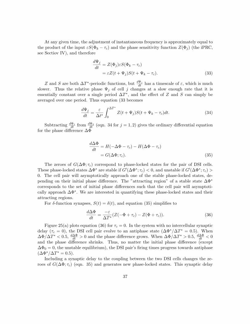
Figure 25(a) plots equation (36) for τc = 0. In the system with no intercellular synapticdelay (τc = 0), the DSI cell pair evolve to an antiphase state (∆Φ∗/∆T ∗ = 0.5). When∆Φ/∆T ∗ < 0.5, d∆Φ
dt > 0 and the phase difference grows. When ∆Φ/∆T ∗ > 0.5, d∆Φdt < 0
and the phase difference shrinks. Thus, no matter the initial phase difference (except∆Φ0 = 0, the unstable equilibrium), the DSI pair’s firing times progress towards antiphase(∆Φ∗/∆T ∗ = 0.5).
Including a synaptic delay to the coupling between the two DSI cells changes the ze-roes of G(∆Φ; τc) (eqn. 35) and generates new phase-locked states. This synaptic delay
37

causes bistability in phase-locking behavior. Depending on the initial phase differencebetween the two DSI cells, the pair will evolve to either antiphase ∆Φ∗/∆T ∗ = 0.5 orsynchrony ∆Φ∗/∆T ∗ = 0 or 1. Note that since phase is ∆T ∗-periodic, phases 0 and ∆T ∗
are equivalent. In Figure 25, the arrows point towards points that correspond to stablephase-locked states and away from points that correspond to unstable phase-locked states.If the initial phase difference between the two cells is exactly the phase corresponding tothe unstable steady states, the cells will remain at that phase difference, but any pertur-bation to the system will cause the cells to evolve to one of the stable states. In Figure25(b), τc = 0.15∆T ∗, and the attracting region of the antiphase state is larger than that ofthe synchronous state In Figure 25(c), τc = 0.35∆T ∗, and the opposite is true. In Figure25(d), τc = 0.5 and the two unstable fixed points have coalesced with the stable fixed pointat phase ∆Φ∗/∆T ∗ = 0.5; thus, with any initial phase difference the cell pair will evolve tosynchronous activity (∆Φ∗/∆T ∗ = 0). This pattern of growing and shrinking attractingregions of the antiphase and synchronous states repeats periodically as the synaptic delayτc is increased past ∆T ∗.
38
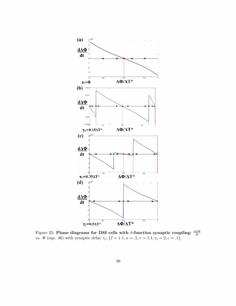
Figure 25: Phase diagrams for DSI cells with δ-function synaptic coupling: d∆Φdt
vs. Φ (eqn. 36) with synaptic delay τc, I = 1.1, α = .5, τ = 1.1, τs = 2, ε = .1.
39

Figure 26: Phase diagrams for DSI cells with exponentially-decaying synapticcoupling: d∆Φ
dt vs. Φ (eqn. 35) with synaptic delay τc, I = 1.1, α = .5, τ = 1.1, τs =2, ε = .1, τsc = 100.
40

We can summarize these changes in phase-locking behavior as τc is varied in bifurcationdiagrams
Figure 27: This bifurcation diagram shows the changing stabilities of Φ∗ for the δ-functionsynaptic coupling as the synaptic delay τc is varied, I = 1.1, α = .5, τ = 1.1, τs = 2, ε = .1
The bifurcation diagram in Figure 27 summarizes the appearance and disappearanceof phase-locked states Φ∗ as the synaptic delay τc is varied for the coupled DSI cells withδ-function synaptic coupling.
With no delay (τc = 0), the only stable phase-locked state is antiphase (synchronyis unstable). As the delay increases, the synchronous state gains stability and a pair ofunstable steady states emerge. As the delay approaches phase 0.5, the attracting region Bof the synchronous phase-locked state grows and the attracting region A of the antiphasephase-locked state shrinks. At τc = 0.5∆T ∗, there is a degenerate pitchfork bifurcation asthe unstable states coalesce with the stable antiphase state causing antiphase to go unstableat τ = 0.5∆T ∗, which makes the only stable phase-locked state of this system synchronous.As τc increases past 0.5∆T ∗, the antiphase state immediately regains stability and theunstable steady states reemerge. As τc approaches ∆T ∗, the attracting region B of thesynchronous phase-locked state shrinks and the attracting region A of the antiphase phase-locked state grows. After τc = ∆T ∗, the pattern of growing and shrinking attracting regionsA and B (with a sequence of degenerate pitchfork bifurcations) repeats ∆T ∗-periodically.For any delay τc (except τc = 0, 0.5∆T ∗, ∆T ∗, 1.5∆T ∗, . . . ), there is bistability in phase-locking behavior, albeit with unequally-sized attracting regions for the two fixed phasedifferences.
41
Figure 28: This bifurcation diagram shows the changing stabilities of Φ∗ for theexponentially-decaying synaptic coupling as the synaptic delay τc is varied, I = 1.1, α =.5, τ = 1.1, τs = 2, ε = .1, τsc = 100
The bifurcation diagram in Figure 28 shows the appearance and disappearance of phase-locked states Φ∗ as the synaptic delay τc is varied for the coupled cells with exponentially-decaying synaptic coupling (with decay rate τsc = 100). There are two important differ-ences between the bifurcation diagrams for the exponentially-decaying synaptic couplingcase and the δ-function synaptic coupling case (compare Figures 28 and 27). First, theattracting region A of the antiphase phase-locked state does not begin to shrink untilτc ≈ .25∆T ∗. Second, the pitchfork bifurcation is degenerate in the case of δ-functionsynaptic coupling, see Figure 27. At τc = 0.5∆T ∗, the unstable states coalesce withthe stable antiphase state causing antiphase to go unstable, which makes the only stablephase-locked state of this system synchronous. This remains the only stable phase-lockedstate until τc ≈ 0.7∆T ∗. Then antiphase regains stability, and the attracting region B ofthe synchronous phase-locked state shrinks and the attracting region A of the antiphasephase-locked state grows. After τc = ∆T ∗, this pattern of shrinking and growing attractingregions A and B (with a sequence of pitchfork bifurcations) repeats periodically. Modelingthe synaptic coupling with exponentially-decaying over δ-function synapses leads to morerobust cases of monostability in phase-locked states.
Altering the individual DSI cell parameters (I, τ ,α, τs) changes the iPRCs quantita-tively, but does not qualitatively change the phase-locking states of the two-cell system.The general results of this section hold true for any set of parameters that generates aniPRC of the same nature as in the previous section (i.e., for 1.01 < I < 1.5, .1 < α < .9,.1 < τ < 2, .1 < τs ≤ 3). The parameters that affect the phase-locking are entirely con-tained in the synaptic connections between the two cells. Increasing the synaptic delay τcchanges the stability of phase-locked antiphase and synchrony and also generates unstablestates (see Figures 27-28), while increasing the synaptic decay rate τsc smooths out thedynamics of equation (35) (compare Figures 25 and 26) and quantitatively changes the bi-furcation diagram (compare Figure 27 and 28). Changing the synaptic strength ε rescalesequation (35) but has no effect on the phase-locking states and their stability as long as itremains weak (ε << 1).
42

12 Conclusion
In this study, we predict how a neural population with a negative feedback loop oscillates ata characteristic period, responds to perturbations, and synchronizes its oscillatory activitywith neighboring groups by using an idealized model of the system, the DSI cell model. TheDSI cell’s characteristic period arises from cellular and synaptic parameters. Generally,decreasing the bias current or increasing the effects of the “autapse” (via increasing itsstrength, slowing its decay rate, or timing it later) leads to a longer characteristic period.These parameters also affect the DSI cell’s phase sensitivity function (iPRC). Increasingthe strength of the autapse or timing the self-inhibition later in the cell’s firing cycle leadsto an overall decrease in cell’s sensitivity, while decreasing the bias current or increasingthe decay rate of the autapse typically decreases the sensitivity of the cell to earlier-timedperturbations and increases the sensitivity of the cell to later-timed perturbation.
Mutually-inhibiting DSI cell pairs typically tend to synchronize their firing times inantiphase when there are no synaptic delays, however the presence of synaptic delays canproduce in-stable phase activity or bistability between antiphase and in-phase phase-lockingstates. The cellular and synaptic feedback parameters for the individual DSI cells inves-tigated in the earlier sections have quantitative, but not qualitative, effects on the phase-locking behavior of the pair. Synaptic coupling with slow kinetics (exponentially-decayingsynapses) leads to quantitatively different phase-locking behavior than with synapses withfaster kinetics (δ-function synapses). Specifically, the exponentially-decaying synaptic cou-pling produces more robust monostability in phase-locking behavior, i.e., there are moresynaptic delay values that yield a single stable phase-locked state. Monostability in phase-locked states allows the synchronized oscillations to robustly perform a stable rhythmicrole in specific neural networks, whereas bistability in phase-locked states creates neural“switches “, where the initial phase difference ”switches” the neuron pair to one of thephase-locked states, allowing the system to “remember” input.
The DSI cell has a longer characteristic period and is much less sensitive to weakperturbations than the standard LIF cell with similar parameters. It is far less sensitivethan an LIF cell with the same characteristic period, thus the DSI cell model is more thanjust a standard LIF cell with a longer period. However, the phase-locking behavior ofthe DSI cell is qualitatively, but not quantitatively, similar to phase-locking in mutually-inhibiting LIF cells (without delayed negative feedback), and it would appear that thisqualitative behavior is predominantly determined by the coupling model between the cells.Using a more realistic model of the synaptic coupling between the DSI cells may lead tosignificant qualitative differences and should be investigated further to determine whetheror not the DSI cell model is a good approximation of the behavior of neural systems withdelayed negative feedback.
43

References
[1] J.C. Brumberg and B. S. Gutkin. Cortical pyramidal cells as non-linear oscillators:Experiment and spike-generation theory. Brain Research, (1171):122–137, 2007.
[2] G. B. Ermentrout and D. H. Terman. Mathematical Foundations of Neuroscience,volume 35 of Interdisciplinary Applied Mathematics. Springer, 2010.
[3] J. Foss, A. Longtinm, B. Mensour, and J. Milton. Multistability and delayed recurrentloops. Physical Review Letters, 76(4):708–711, February 1965.
[4] A. L. Hodgkin and A. F. Huxley. A quantitative description of membrane currentand its application to conduction and excitation in nerve. The Journal of Physiology,117(4):500–544, 1952.
[5] F.C. Hoppensteadt and E.M. Izhikevich. Weakly Connected Neural Networks. Numberv. 126 in Applied Mathematical Sciences. Springer New York, 1997.
[6] C. L. Johnson. Phase response properties and phase-locking in neural systems withdelayed negative feedback. Explorations - UC Davis Undergraduate Research Journal,2015.
[7] B. Katz and R. Miledi. The measurement of synaptic delay, and the time course ofacetylcholine release at the neuromuscular junction. Proceedings of the Royal Societyof London. Series B. Biological Sciences, 161(985):483–495, February 1965.
[8] L. Melloni, C. Molina, M. Pena, D. Torres, W. Singer, and E. Rodriguez. Synchro-nization of neural activity across cortical areas correlates with conscious perception.The Journal of Neuroscience, 27:2858–2865, 2007.
[9] R. Miller. Oscillatory Event-Related Brain Dynamics, volume 271 of NATO ASI Se-ries, chapter What is the contribution of axonal conduction delay to temporal structurein brain dynamics?, pages 53–57. Springer US, 1994.
[10] C. Morris and H. Lecar. Voltage oscillations in the barnacle giant muscle fiber. Journalof Biophysics, 35:193–213, 1981.
[11] A. Engel P. Konig and W. Singer. Relation between oscillatory activity and long rangesynchronization in cat visual cortex. Proceedings of the National Academy of Sciencesof the United States of America, 92:290–294, 1995.
[12] M. A. Schwemmer and T. J. Lewis. The theory of weakly coupled oscillators. InR. J. Butera N.W. Schultheiss, A. Prinz, editor, PRCs in Neuroscience: Theory, Ex-periment, and Analysis, volume 6 of Springer Series in Computational Neuroscience,pages 3–31. Springer, 2012.
44

[13] S. H. Strogatz and I. Stewart. Coupled oscillators and biological synchronization.Scientific American, pages 102–109, December 1993.
[14] S.H. Strogatz. Sync: How Order Emerges from Chaos In the Universe, Nature, andDaily Life. Hachette Books, 2012.
[15] C. Zhang and T. J. Lewis. Phase response properties of half-center oscillators. Journalof Computational Neuroscience, 35:55–74, 2013.
45
![Azimuthal jet avor tomography with CUJET2.0 of nuclear ...However, the \surprising transparency" [47] of QGP produced at LHC severely challenged the xed coupling version of the CUJET1.0](https://static.documents.pub/doc/80x56/60f68e2fdf5bc53e88085656/azimuthal-jet-avor-tomography-with-cujet20-of-nuclear-however-the-surprising.jpg)


