This is an Open Access article, distributed under the terms of the Creative Commons Attributionlicence (http://creativecommons.org/licenses/by/4.0/), which permits unrestricted re-use, distribution,and reproduction in any medium, provided the original work is properly cited.doi:10.1017/jfm.2020.973
Coupling rheology and segregation ingranular flows
T. Barker1,2, M. Rauter3,4, E. S. F. Maguire1, C. G. Johnson1
and J. M. N. T. Gray1,†
1Department of Mathematics and Manchester Centre for Nonlinear Dynamics, University of Manchester,Oxford Road, Manchester M13 9PL, UK
2School of GeoSciences and Institute for Infrastructure and Environment, University of Edinburgh,King’s Buildings, Edinburgh EH9 3JL, UK
3Department of Natural Hazards, Norwegian Geotechnical Institute, Oslo N-0806, Norway4Department of Mathematics, University of Oslo, Oslo N-0851, Norway
(Received 6 March 2020; revised 19 October 2020; accepted 2 November 2020)
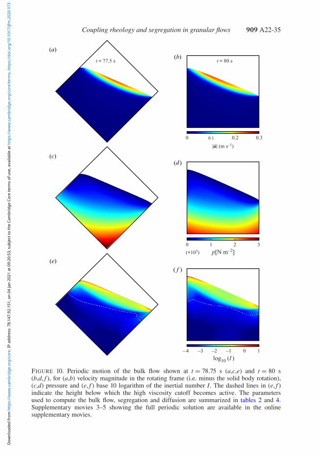
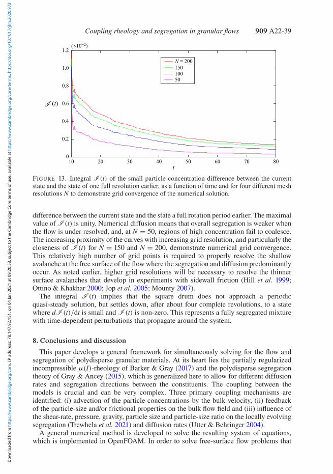
During the last fifteen years there has been a paradigm shift in the continuum modellingof granular materials; most notably with the development of rheological models, such asthe μ(I)-rheology (where μ is the friction and I is the inertial number), but also withsignificant advances in theories for particle segregation. This paper details theoretical andnumerical frameworks (based on OpenFOAM®) which unify these currently disconnectedendeavours. Coupling the segregation with the flow, and vice versa, is not only vitalfor a complete theory of granular materials, but is also beneficial for developingnumerical methods to handle evolving free surfaces. This general approach is based on thepartially regularized incompressible μ(I)-rheology, which is coupled to the gravity-drivensegregation theory of Gray & Ancey (J. Fluid Mech., vol. 678, 2011, pp. 353–588).These advection–diffusion–segregation equations describe the evolving concentrations ofthe constituents, which then couple back to the variable viscosity in the incompressibleNavier–Stokes equations. A novel feature of this approach is that any number of differentlysized phases may be included, which may have disparate frictional properties. Furtherinclusion of an excess air phase, which segregates away from the granular material, thenallows the complex evolution of the free surface to be captured simultaneously. Threeprimary coupling mechanisms are identified: (i) advection of the particle concentrationsby the bulk velocity, (ii) feedback of the particle-size and/or frictional properties on thebulk flow field and (iii) influence of the shear rate, pressure, gravity, particle size andparticle-size ratio on the locally evolving segregation and diffusion rates. The numericalmethod is extensively tested in one-way coupled computations, before the fully coupledmodel is compared with the discrete element method simulations of Tripathi & Khakhar(Phys. Fluids, vol. 23, 2011, 113302) and used to compute the petal-like segregationpattern that spontaneously develops in a square rotating drum.
Despite nearly all natural and man-made granular materials being composed of grains ofvarying size, shape and frictional properties, the majority of continuum flow modelling haslargely been restricted to perfectly monodisperse aggregates. The purpose of this work istherefore to extend the current granular flow models by introducing multiple phases, withdifferent properties, and to model inter-phase segregation. Coupling the flow rheologyto the local constituent concentrations is important because the mobility of a granularflow is strongly affected by the local frictional properties of the grains. In turn, the bulkflow controls the strength and direction of the segregation as well as the advection of thegranular phases.
Striking examples of segregation induced feedback on the bulk flow are found duringlevee formation (Iverson & Vallance 2001; Johnson et al. 2012; Kokelaar et al. 2014) andfingering instabilities (Pouliquen, Delour & Savage 1997; Pouliquen & Vallance 1999;Woodhouse et al. 2012; Baker, Johnson & Gray 2016b), which commonly occur duringthe run-out of pyroclastic density currents, debris flows and snow avalanches. Many otherexamples of segregation–flow coupling occur in industrial settings (Williams 1968; Gray& Hutter 1997; Makse et al. 1997; Hill et al. 1999; Ottino & Khakhar 2000; Zuriguel et al.2006). Storage silo filling and emptying, stirring mixers and rotating tumblers all havethe common features of cyclic deformation and an ambition of generating well-mixedmaterial. However, experiments consistently suggest that these processes have a tendencyto promote local segregation, which can feedback on the bulk flow velocities. Consideringthe inherent destructive potential of geophysical phenomena and the implications of poorefficiency in industrial mixing, a continuum theory which captures the important physicsof flow and of segregation simultaneously is therefore highly desirable.
To date, the leading approaches for solving coupled flow and segregation have comefrom either discrete particle simulations (Tripathi & Khakhar 2011; Thornton et al.2012) or from depth-averaged equations (Woodhouse et al. 2012; Baker et al. 2016b;Viroulet et al. 2018). Particle simulations, using the discrete element method (DEM),provide important rheological information as evolving velocities, stresses and constituentconcentrations can be directly computed given only minimal approximations. Such resultscan then be used to motivate models for the bulk flow (GDR MiDi 2004; Jop, Forterre& Pouliquen 2006; Singh et al. 2015) and also to form connections between flowand segregation processes (Hill & Fan 2008; Staron & Phillips 2015). Unfortunately,the discrete particle approach is naturally limited by computational expense as manyflows of interest include such a large number of particles that direct DEM calculationsare unfeasible. Recently efforts have been made to overcome this limitation with thedevelopment of hybrid schemes (e.g. Yue et al. 2018; Xiao et al. 2019) which couplediscrete particle dynamics to continuum solvers, but these approaches naturally invokeadditional complexity and new assumptions are required in order to map properly andconsistently between the somewhat disparate approaches.
Depth-averaged models, which reduce the full three-dimensional flow to twodimensions by integrating though the depth and assuming shallowness, lead to efficientnumerical codes which are widely used in geophysical modelling (see e.g. Grigorian,Eglit & Iakimov 1967; Savage & Hutter 1989; Iverson 1997; Gray, Wieland & Hutter1999; Pouliquen & Forterre 2002; Sheridan et al. 2005; Mangeney et al. 2007; Christen,Kowalski & Bartelt 2010; Gray & Edwards 2014; Delannay et al. 2017; Rauter & Tukovic2018; Rocha, Johnson & Gray 2019). However, depth-averaged approaches are limitedto geometries in which there is a clear dimension that remains shallow throughout thedynamics. This approximation holds well for thin flows on inclined planes and for flows
Coupling rheology and segregation in granular flows 909 A22-3
over certain gradually varying terrain, but breaks down in many flows of practical interest,such as those in hoppers, silos and rotating drums.
Historical attempts to construct three-dimensional continuum models for monodispersegranular materials focused on quasi-static deformations and lead to elasto-plasticformulations of models such as the Drucker–Prager yield condition (Lubliner 2008) andcritical state soil mechanics (Schofield & Wroth 1968). Despite successes in modellingthe point of failure of materials under load, calculations of the subsequent time-dependentflow proved to be problematic, because the results are grid-size dependent. Schaeffer(1987) showed that this was because the underlying equations are mathematically ill posed,i.e. in the small wavelength limit the growth rate of linear instabilities becomes unboundedin certain directions.
Despite the Mohr–Coulomb/Drucker–Prager plasticity theory being designed for theflow of monodisperse grains, the grain diameter d does not appear in the constitutivemodel. It can be incorporated by making the friction μ a function of the non-dimensionalinertial number, which is defined as
I = dγ√p/ρ∗
, (1.1)
where γ is the shear rate, p is the pressure and ρ∗ is the intrinsic grain density (Savage1984; Ancey, Coussot & Evesque 1999; GDR MiDi 2004). Jop et al. (2006) generalizedthe scalar μ(I)-rheology to tensorial form. The resultant incompressible μ(I)-rheologyleads to a significantly better posed system of equations (Barker et al. 2015). For the μ(I)curve suggested by Jop, Forterre & Pouliquen (2005), the equations are well posed for alarge range of intermediate values of I and are only ill posed for very low or relatively highinertial numbers.
Barker & Gray (2017) derived a new functional form for the μ(I) relation, whichis known as the partially regularized μ(I)-rheology. This ensures well posedness for0 < I < Imax , where Imax is a very large value, and leads to stable and reliable numericalschemes. It also provides a better fit to experimental (Holyoake & McElwaine 2012; Barker& Gray 2017) and DEM data (Kamrin & Koval 2012) than the original μ(I) curve, but alsointroduces a creep state (i.e. μ = 0 when I = 0) so the granular material no longer has ayield stress. It is possible to formulate well-posed models with a yield stress by introducingbulk compressibility (Barker et al. 2017; Schaeffer et al. 2019) or non-locality (Henann &Kamrin 2013). However, in this paper the partially regularized μ(I)-rheology is chosen forthe bulk flow, both for simplicity and because it is most readily compatible with existingnumerical methods and particle segregation models.
Initially well-mixed granular materials have a strong propensity of ordering spatiallywhen they undergo flow. Chief among these effects is that of particle-size segregation,made famous through the moniker ‘the Brazil nut effect’ (Rosato et al. 1987), wherebyparticles move relative to the bulk flow based on their size compared with their neighbours.The resultant vertical distribution, in which larger particles are often concentrated at thesurface of a flow, can also be observed in many geophysical mass flows, forming so-calledinversely graded deposits (e.g. Middleton 1970; Festa et al. 2015). The origin of thiseffect was explained through statistical entropic arguments by Savage & Lun (1988) whoproposed a means of ‘kinetic sieving’ (Middleton 1970) in which smaller grains are morelikely to fall (by gravity) into voids that are created as layers of particles are shearedover one another. Force imbalances then drive particles out of the denser layer, which isknown as ‘squeeze expulsion’. The combination of kinetic sieving and squeeze expulsionproduces a net upward motion of large particles as the smaller grains percolate downwards.
These concepts formed the basis of the theory of Gray & Thornton (2005) who focused onthis form of gravity-driven segregation in granular free-surface flows. The theory was laterextended by Gray & Chugunov (2006), in order to account for diffusive mixing, and hasbeen successfully applied to a range of gravity-driven flows (Gray 2018). However, Fan &Hill (2011) found that the direction of segregation was not always aligned with the vectorof gravitational acceleration. Instead gradients in kinetic stress were found to drive andorient segregation in a range of geometries (Hill & Tan 2014). These findings have sinceinspired many investigations into the micromechanical origin of size segregation (Staron& Phillips 2015; Guillard, Forterre & Pouliquen 2016; van der Vaart et al. 2018), but aunified and compelling theory is still lacking.
In order to accommodate different models for size segregation and different flowrheologies, this paper first introduces a very general framework for multi-componentflows in § 2. In particular, the multicomponent segregation theory of Gray & Ancey(2011) is generalized to allow sub-mixtures to segregate in different directions and withdiffering diffusion rates. In § 3 the three primary coupling mechanisms are discussedin detail. Section 4 documents the general numerical method, which is then extensivelytested against the one-way coupled simulations in § 5. Two-way fully coupled simulationsare then presented for flow down an inclined plane, in § 6, and in § 7 simulations areperformed for a square rotating drum. The new experimental segregation law of Trewhela,Ancey & Gray (2021) is tested against the steady-state DEM solutions of Tripathi &Khakhar (2011) in § 6.3 and then used in § 7 for the rotating drum simulations, whichare able to spontaneously generate petal-like patterns that have previously been seen in theexperiments of Hill et al. (1999), Ottino & Khakhar (2000) and Mounty (2007).
2. Governing equations
2.1. The partially regularized μ(I)-rheology for the bulk flowThe granular material is assumed to be composed of a mixture of particles that may differin size, shape and surface properties, but have the same intrinsic particle density ρ∗. If thesolids volume fractionΦ is constant, which is a reasonable first approximation (GDR MiDi2004; Tripathi & Khakhar 2011; Thornton et al. 2012), then the bulk density ρ = Φρ∗ isconstant and uniform throughout the material. Mass balance then implies that the bulkvelocity field u is incompressible
∇ · u = 0, (2.1)
where ∇ is the gradient and · is the dot product. The momentum balance is
ρ
(∂u∂t
+ u · ∇u)
= −∇p + ∇ · (2ηD)+ ρg, (2.2)
where p is the pressure, η is the viscosity, D = (∇u + (∇u)T)/2 is the strain-ratetensor and g is the gravitational acceleration. Assuming alignment of the shear-stressand strain-rate tensors the μ(I)-rheology (Jop et al. 2006) implies that the granularviscosity is
η = μ(I)p2‖D‖ , (2.3)
where the second invariant of the strain-rate tensor is defined as
Coupling rheology and segregation in granular flows 909 A22-5
and the inertial number, defined in (1.1), in this notation becomes
I = 2d‖D‖√p/ρ∗
. (2.5)
The meaning of the particle size d in a polydisperse mixture will be clarified in § 3.2.Note that this paper is restricted to two-dimensional deformations with an isotropicDrucker–Prager yield surface. However, as shown by Rauter, Barker & Fellin (2020), thisframework can be extended to include three-dimensional deformations through furthermodification of the granular viscosity i.e. dependence on det(D).
The viscosity (2.3) is a highly nonlinear function of the inertial-number-dependentfriction μ = μ(I), pressure p and the second invariant of the strain rate ‖D‖. Barker et al.(2015) examined the linear instability of the system, to show that the growth rate becomesunbounded in the high wavenumber limit, and hence the incompressible μ(I)-rheology ismathematically ill posed, when the inequality
4(
Iμ′
μ
)2
− 4(
Iμ′
μ
)+ μ2
(1 − Iμ′
2μ
)> 0, (2.6)
is satisfied, where μ′ = ∂μ/∂I. Ill posedness of this type is not only unphysical, but resultsin two-dimensional time-dependent numerical computations that do not converge withmesh refinement (see e.g. Barker et al. 2015; Barker & Gray 2017; Martin et al. 2017).If the friction is not inertial number dependent (μ = const.) the ill-posedness condition(2.6) is satisfied for all inertial numbers and the system of equations is always ill posed(Schaeffer 1987). The equations are also ill posed if the friction μ is a decreasing functionof I, since all the terms in (2.6) are strictly positive.
The original form of the μ(I)-curve proposed by Jop et al. (2005) is a monotonicallyincreasing function of I starting at μs at I = 0 and asymptoting to μd at large I,
μ(I) = μsI0 + μdII0 + I
, (2.7)
where I0 is a material specific constant. The inertial number dependence in (2.7) givesthe rheology considerably better properties than the original, constant friction coefficient,Mohr–Coulomb/Drucker–Prager theory. Provided μd − μs is large enough, the system iswell-posed when the inertial number lies in a large intermediate range of inertial numbersI ∈ [IN
1 , IN2 ]. The equations are, however, ill posed if either the inertial number is too low
I < IN1 or too high I > IN
2 , or if μd − μs is not large enough. For the parameter valuesgiven in table 1 the μ(I) rheology is well posed for I ∈ [0.00397, 0.28016].
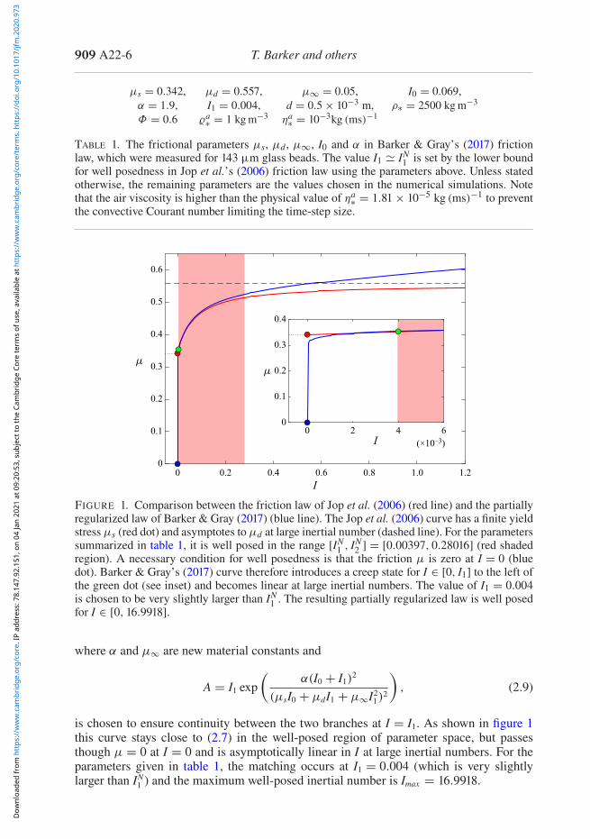
The range of well posedness was extended by Barker & Gray (2017) to 0 ≤ I ≤ Imax ,where Imax is a large maximal value, by changing the shape of the μ(I)-curve. This paperuses the μ(I)-curve proposed by Barker & Gray (2017)
μs = 0.342, μd = 0.557, μ∞ = 0.05, I0 = 0.069,α = 1.9, I1 = 0.004, d = 0.5 × 10⁻³ m, ρ∗ = 2500 kg m−3
Φ = 0.6 �a∗ = 1 kg m−3 ηa∗ = 10−3kg (ms)−1
TABLE 1. The frictional parameters μs, μd, μ∞, I0 and α in Barker & Gray’s (2017) frictionlaw, which were measured for 143 μm glass beads. The value I1 IN
1 is set by the lower boundfor well posedness in Jop et al.’s (2006) friction law using the parameters above. Unless statedotherwise, the remaining parameters are the values chosen in the numerical simulations. Notethat the air viscosity is higher than the physical value of ηa∗ = 1.81 × 10⁻⁵ kg (ms)−1 to preventthe convective Courant number limiting the time-step size.
0.6
0.5
0.4
0.3
0.2
0.1
0
0.4
0.3
0.2
0.1
00
0 0.2 0.4 0.6
I
μμ
I
0.8 1.0 1.2
2 4 6
(×10–3)
FIGURE 1. Comparison between the friction law of Jop et al. (2006) (red line) and the partiallyregularized law of Barker & Gray (2017) (blue line). The Jop et al. (2006) curve has a finite yieldstressμs (red dot) and asymptotes toμd at large inertial number (dashed line). For the parameterssummarized in table 1, it is well posed in the range [IN
1 , IN2 ] = [0.00397, 0.28016] (red shaded
region). A necessary condition for well posedness is that the friction μ is zero at I = 0 (bluedot). Barker & Gray’s (2017) curve therefore introduces a creep state for I ∈ [0, I1] to the left ofthe green dot (see inset) and becomes linear at large inertial numbers. The value of I1 = 0.004is chosen to be very slightly larger than IN
1 . The resulting partially regularized law is well posedfor I ∈ [0, 16.9918].
where α and μ∞ are new material constants and
A = I1 exp(
α(I0 + I1)2
(μsI0 + μdI1 + μ∞I21)
2
), (2.9)
is chosen to ensure continuity between the two branches at I = I1. As shown in figure 1this curve stays close to (2.7) in the well-posed region of parameter space, but passesthough μ = 0 at I = 0 and is asymptotically linear in I at large inertial numbers. For theparameters given in table 1, the matching occurs at I1 = 0.004 (which is very slightlylarger than IN
1 ) and the maximum well-posed inertial number is Imax = 16.9918.
Coupling rheology and segregation in granular flows 909 A22-7
The partially regularized μ(I)-rheology not only ensures well posedness for I < Imax ,but it also provides better fitting to experimental and DEM results. For instance, relative to(2.7) the newμ(I)-curve (2.8) predicts higher viscosities for large values of I, as seen in thechute flow experiments of Holyoake & McElwaine (2012) and Barker & Gray (2017). Forlow values of I, the partially regularized μ(I)-rheology predicts very slow creeping flow,since μ → 0 as I → 0. This behaviour is seen, to a certain extent, in DEM simulations(Kamrin & Koval 2012; Singh et al. 2015) and has been postulated by Jerolmack & Daniels(2019) to play an important role in soil creep. The lack of a yield stress may, however, beviewed as a disadvantage of the theory. It is important to note that by allowing some bulkcompressibility, it is possible to formulate granular rheologies that are always well posedmathematically (Barker et al. 2017; Heyman et al. 2017; Goddard & Lee 2018; Schaefferet al. 2019) and support a yield stress.
2.2. Generalized polydisperse segregation theoryThe granular material is assumed to be composed of a finite number of grain-size classes,or species ν, which have different sizes dν , but all have the same intrinsic density ρν∗ = ρ∗.Note that the inclusion of density differences between the particles implies that the bulkvelocity field is compressible, which significantly complicates the theory (Tripathi &Khakhar 2013; Gray & Ancey 2015; Gilberg & Steiner 2020) and is therefore neglected.Even for a bidisperse mixture of particles of the same density, the grains can pack slightlydenser in a mixed state than in a segregated one (Golick & Daniels 2009). However,the DEM simulations (Tripathi & Khakhar 2011; Thornton et al. 2012) suggest thesepacking effects are small, and for simplicity, and compatibility with the incompressibleμ(I)-rheology, these solids volume fraction changes are neglected. Each grain-size classis therefore assumed to occupy a volume fraction φν ∈ [0, 1] per unit granular volume,and the sum over all grain sizes therefore equals unity∑
∀νφν = 1. (2.10)
Many models to describe particle segregation have been proposed (see e.g. Bridgwater,Foo & Stephens 1985; Savage & Lun 1988; Dolgunin & Ukolov 1995; Khakhar, Orpe& Hajra 2003; Gray & Thornton 2005; Gray & Chugunov 2006; Fan & Hill 2011;Gray & Ancey 2011; Schlick et al. 2015) and these all have the general form of anadvection–segregation–diffusion equation
∂φν
∂t+ ∇ · (φνu)+ ∇ · F ν = ∇ · Dν
, (2.11)
where F ν is the segregation flux and Dν is the diffusive flux. Provided that these fluxesare independent, this formulation is compatible with the bulk incompressibility provided∑
∀νF ν = 0, and
∑∀ν
Dν = 0. (2.12a,b)
The form of the segregation flux is motivated by early bidisperse models (Bridgwateret al. 1985; Dolgunin & Ukolov 1995; Gray & Thornton 2005). These all had the propertythat the segregation shut off when the volume fraction of either species reached zero.This is satisfied if the segregation flux for species ν and λ is proportional to φνφλ.In polydisperse systems, Gray & Ancey (2011) proposed that the segregation flux for
species ν was simply the sum of the bidisperse segregation fluxes with all the remainingconstituents λ. This paper proposes a significant generalization of this concept, by allowingthe local direction of segregation to be different for each bidisperse sub-mixture, so thatthe segregation flux takes the general polydisperse form
F ν =∑
∀λ /= νfνλφνφλeνλ, (2.13)
where fνλ is the segregation velocity magnitude and eνλ is the unit vector in the directionof segregation, for species ν relative to species λ. This segregation flux function satisfiesthe summation constraint (2.12a,b) provided
fνλ = fλν and eνλ = −eλν. (2.14a,b)
In contrast to the theory of Gray & Ancey (2011) the segregation velocity magnitudeis the same for species ν with species λ and species λ with species ν, and it is insteadthe direction of segregation that now points in the opposite sense. This approach has theproperty that individual sub-mixtures may segregate in different directions, which allowsthe theory to be applied to polydisperse problems where gravity-driven segregation (e.g.Gray 2018) competes against segregation driven by gradients in kinetic stress (Fan &Hill 2011). This would require the constituent vector momentum balance to be solvedin order to determine the resultant magnitude and direction of segregation (Hill & Tan2014; Tunuguntla, Weinhart & Thornton 2017). In this paper the inter-particle segregationis always assumed to align with gravity. However, the direction of segregation for theparticles and air can be chosen to be different. This proves to be advantageous in thenumerical method that will be developed to solve the coupled system of equations in § 4.
It is also very useful in the numerical method to allow the rate of diffusion between thevarious sub-mixtures to be different. By direct analogy with the Maxwell–Stefan equations(Maxwell 1867) for multi-component gas diffusion, the diffusive flux vector is thereforeassumed to take the form
Dν =∑
∀λ /= νDνλ
(φλ∇φν − φν∇φλ) , (2.15)
where Dνλ is the diffusion coefficient of species ν with species λ. Equation (2.15) satisfiesthe summation constraint (2.12a,b), provided Dνλ = Dλν , and reduces to the usual Fickiandiffusion for the case of bidisperse mixtures (see e.g. Gray & Chugunov 2006). For amixture of n distinct species, it is necessary to solve n − 1 separate equations of the form(2.11) together with the summation constraint (2.10) for the n concentrations φν , assumingthat the bulk velocity field u is given.
In the absence of diffusion, concentration shocks form naturally in the system (see e.g.Gray & Thornton 2005; Thornton, Gray & Hogg 2006; Gray & Ancey 2011). The jumpsin concentration across such boundaries can be determined using jump conditions that arederived from the conservation law (2.11) (see e.g. Chadwick 1976). These jump conditionsare also useful when formulating boundary conditions with diffusion. The most generalform of the jump condition for species ν is
Coupling rheology and segregation in granular flows 909 A22-9
where n is the normal to the shock, vn is the normal speed of the shock and the jumpbracket [[ ]] is the difference of the enclosed quantity on the forward and rearward sides ofthe shock. In particular, if the flow is moving parallel to a solid stationary wall, then thejump condition reduces to the one-sided boundary condition∑
∀λ /= νfνλφνφλeνλ · n =
∑∀λ /= ν
Dνλ
(φλ∇φν − φν∇φλ) · n. (2.17)
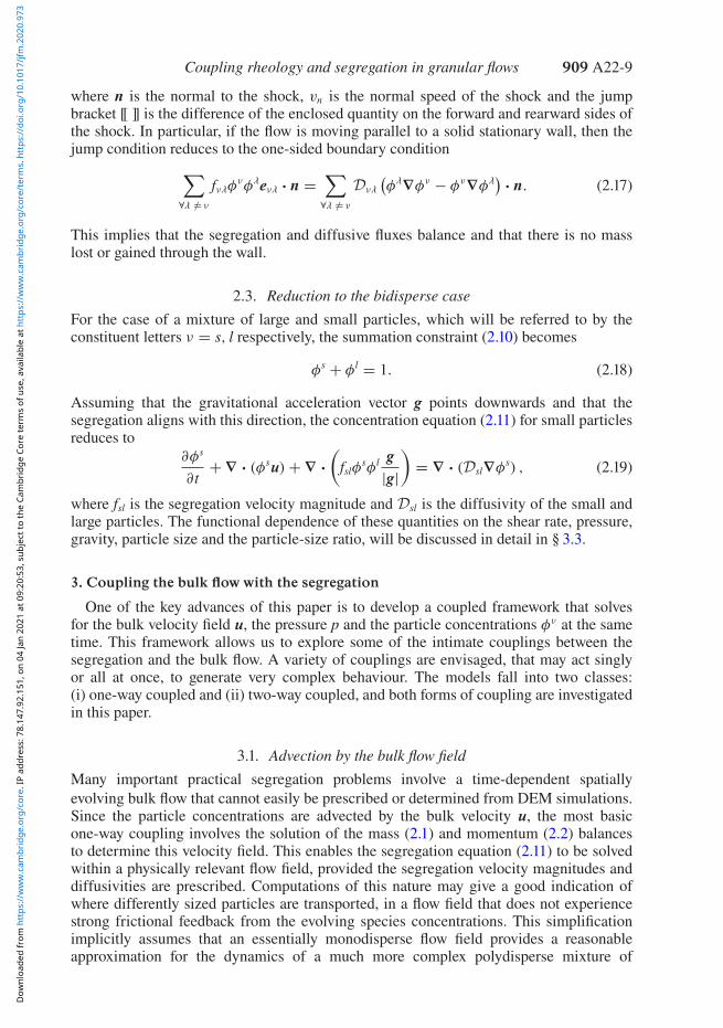
This implies that the segregation and diffusive fluxes balance and that there is no masslost or gained through the wall.
2.3. Reduction to the bidisperse caseFor the case of a mixture of large and small particles, which will be referred to by theconstituent letters ν = s, l respectively, the summation constraint (2.10) becomes
φs + φl = 1. (2.18)
Assuming that the gravitational acceleration vector g points downwards and that thesegregation aligns with this direction, the concentration equation (2.11) for small particlesreduces to
∂φs
∂t+ ∇ · (φsu)+ ∇ ·
(fslφ
sφl g|g|
)= ∇ · (Dsl∇φs) , (2.19)
where fsl is the segregation velocity magnitude and Dsl is the diffusivity of the small andlarge particles. The functional dependence of these quantities on the shear rate, pressure,gravity, particle size and the particle-size ratio, will be discussed in detail in § 3.3.
3. Coupling the bulk flow with the segregation
One of the key advances of this paper is to develop a coupled framework that solvesfor the bulk velocity field u, the pressure p and the particle concentrations φν at the sametime. This framework allows us to explore some of the intimate couplings between thesegregation and the bulk flow. A variety of couplings are envisaged, that may act singlyor all at once, to generate very complex behaviour. The models fall into two classes:(i) one-way coupled and (ii) two-way coupled, and both forms of coupling are investigatedin this paper.
3.1. Advection by the bulk flow fieldMany important practical segregation problems involve a time-dependent spatiallyevolving bulk flow that cannot easily be prescribed or determined from DEM simulations.Since the particle concentrations are advected by the bulk velocity u, the most basicone-way coupling involves the solution of the mass (2.1) and momentum (2.2) balancesto determine this velocity field. This enables the segregation equation (2.11) to be solvedwithin a physically relevant flow field, provided the segregation velocity magnitudes anddiffusivities are prescribed. Computations of this nature may give a good indication ofwhere differently sized particles are transported, in a flow field that does not experiencestrong frictional feedback from the evolving species concentrations. This simplificationimplicitly assumes that an essentially monodisperse flow field provides a reasonableapproximation for the dynamics of a much more complex polydisperse mixture of
particles, and that there is no feedback of this local flow field on the segregation anddiffusion rates. This simple coupling is investigated in § 5 for a time-dependent spatiallyevolving flow down an inclined plane. Importantly, this simple one-way coupling alsoenables the accuracy of the numerical method to be tested against known exact travellingwave and steady-state solutions for the bulk flow field and the particle concentrations.In general, the particle concentrations are always transported by the bulk flow field, sothis mechanism is also active in models with more complex couplings, which will beinvestigated in §§ 6 and 7.
3.2. Segregation induced frictional feedback on the bulk flowEach distinct granular phase may have differing particle size, shapes or surface properties,that lead to different macroscopic friction and/or rheological parameters. In this next stageof coupling these rheological differences are built into the model, so that the evolvingparticle concentrations feedback on the bulk flow through the evolving macroscopicfriction of the mixture. There are two basic ways to introduce this coupling.
A key finding of the μ(I)-rheology (GDR MiDi 2004) was that the inertial number(2.5) is a function of the particle size d. This is clearly defined in a monodispersemixture, but an important generalization is needed for polydisperse systems. Based onDEM simulations of bidisperse two-dimensional assemblies of disks, Rognon et al. (2007)proposed an inertial number in which the particle size d was replaced by the local volumefraction weighted average particle size d. The same law was also proposed by Tripathi &Khakhar (2011) and shown to agree with three-dimensional DEM simulations of spheres.Generalizing this concept to polydisperse systems, implies that the average particle size
d =∑∀νφνdν, (3.1)
evolves as the local concentrations φν of each particle species change. As a result, giventhe same local shear rate 2‖D‖, pressure p and intrinsic grain density ρ∗, the new inertialnumber
I = 2d‖D‖√p/ρ∗
(3.2)
will be larger for a mixture composed of larger particles than one made of smaller grains.As well as differences in size, the particles may also differ in shape and/or surface
properties. A prime example of this are segregation induced fingering instabilities, whichdevelop with large angular (resistive) particles and finer spherical particles (Pouliquenet al. 1997; Pouliquen & Vallance 1999; Woodhouse et al. 2012; Baker et al. 2016b). Theeffect of particle shape and surface properties can certainly be modelled in monodisperseflows by changing the assumed macroscopic frictional parameters (see e.g. Pouliquen &Forterre 2002; Forterre 2006; Edwards et al. 2019; Rocha et al. 2019). Furthermore, theresults of Baker et al.’s (2016b) granular fingering model suggest that a good approach isto assume that each phase satisfies a monodisperse friction law μν = μν(I) of the form(2.8) and then compute the effective friction by the weighted sum of these laws, i.e.
Coupling rheology and segregation in granular flows 909 A22-11
On the other hand, it is also possible to assume that there is a single μ(I)-curve, given by(2.8), but that the parameters in it evolve as the mixture composition changes, i.e.
μs =∑∀νφνμνs , μd =
∑∀νφνμνd, μ∞ =
∑∀νφνμν∞, I0 =
∑∀νφνIν0 , (3.4a–d)
where μνs , μνd, μν∞ and Iν0 are the frictional parameters for a pure phase of constituent ν.There is clearly potential for a great deal of complexity here that needs to be explored.However, to the best of our knowledge there are no DEM studies that measure theeffective frictional properties of mixtures of particles of different sizes, shapes and surfaceproperties that could further guide the model formulation. Segregation mobility feedbackon the bulk flow will be investigated further in § 6.
3.3. Feedback of the bulk flow on the segregation rate and diffusivityThe shear rate γ = 2‖D‖, the pressure p, gravity g and the particle properties also enterthe equations more subtly through the functional dependence of the segregation velocitymagnitude fνλ and diffusivity Dνλ in the fluxes (2.13) and (2.15). Even in bidispersegranular mixtures very little is known about their precise functional dependencies.However, dimensional analysis is very helpful in constraining the allowable forms.
Consider a bidisperse mixture of large and small grains of sizes dl and ds, respectively,which have the same intrinsic density ρ∗. The small particles occupy a volume fractionφs = 1 − φl per unit granular volume and the total solids volume fraction isΦ. The systemis subject to a bulk shear stress τ , a pressure p and gravity g, which results in a shear rate γ .Even though these variables are spatially varying, they are considered here as inputs to thesystem, whereas the segregation velocity magnitude fsl and the diffusivity Dsl are outputs.Since there are nine variables, with three primary dimensions (mass, length and time),dimensional analysis implies that there are six independent non-dimensional quantities
μ = τ
p, I = γ d√
p/ρ∗, Φ, P = p
ρ∗gd, R = dl
ds, φs, (3.5a–f )
where d is the volume fraction weighted average grain size defined in (3.1), P is thenon-dimensional pressure and R is the grain-size ratio. For a monodisperse system in theabsence of gravity, only the first three quantities are relevant and GDR MiDi (2004) madea strong case for the friction μ being purely a function of the inertial number I. This led tothe development of the incompressible μ(I)-rheology (GDR MiDi 2004; Jop et al. 2006;Barker & Gray 2017), which is used in this paper.
Using the monodisperse scalings, it follows that in the absence of gravity theself-diffusion of grains should scale as
D ∼ γ d2 F(μ, I, Φ), (3.6)
where F is an arbitrary function of the friction, the inertial number and the solidsvolume fraction, and with no dependence on P, R and φs. In both the incompressibleand compressible μ(I)-rheologies (GDR MiDi 2004; da Cruz et al. 2005; Jop et al. 2006;Forterre & Pouliquen 2008) the friction μ and the solids volume fraction Φ are rigidlybound to the inertial number I, so it is not necessary to retain their dependence in (3.6).However, in the latest well-posed compressible theories (e.g. Barker & Gray 2017; Heymanet al. 2017; Schaeffer et al. 2019) the μ = μ(I) and Φ = Φ(I) laws only hold at steadystate, and so the general form of the diffusivity (3.6) applies.
Utter & Behringer (2004) showed experimentally that the self-diffusion coefficientscaled with the shear rate and the particle size squared. This suggests that the simplestmodel for the diffusion of the grains in a polydisperse system is
Dνμ = Aγ d2, (3.7)
where A = 0.108 is a universal constant (Utter & Behringer 2004) and d is now interpretedas the average, locally evolving, particle size defined in (3.1). Some evidence for this isprovided by the experiments of Trewhela et al. (2021) which show that a single smallintruder in a matrix of large grains performs larger random walks than a single largeintruder in a matrix of fine grains. In general, however, the diffusivity could be multipliedby an arbitrary function of the other non-dimensional quantities in (3.5a–f ).
Gravity-driven percolation (kinetic sieving) and squeeze expulsion (Middleton 1970;Bridgwater et al. 1985; Savage & Lun 1988; Gray & Thornton 2005; Gray 2018) combineto create the dominant mechanism for segregation in dense sheared granular flows.Assuming that the segregation is independent of the diffusion, dimensional analysissuggests that the segregation velocity magnitude in a bidisperse mixture of large and smallparticles should scale as
fsl ∼ γ d G(μ, I, Φ,P,R, φs), (3.8)
where G is an arbitrary function. It has long been known that the segregation velocitymagnitude fsl is strongly dependent on the strain rate and the particle-size ratio (see e.g.Bridgwater et al. 1985; Savage & Lun 1988). Gray & Thornton (2005) also suggestedthat there should be a dependence on gravity. Evidence for this is provided by the factthat granular segregation experiments, with a density matched interstitial fluid, do notsegregate (Vallance & Savage 2000; Thornton et al. 2006), i.e. when gravity is effectivelyreduced, so is the rate of segregation. Inclusion of the gravitational acceleration suggeststhat the segregation velocity magnitude should also be pressure dependent, since g onlyappears in the non-dimensional pressure P. This is supported by the experiments of Golick& Daniels (2009), who observed a dramatic slowing in the segregation rate when theyapplied a normal force on their ring shear cell. This pressure-dependent suppression ofsegregation has been investigated further in the DEM simulations of Fry et al. (2018), whosuggested that the segregation velocity magnitude should scale with the reciprocal of thesquare root of the pressure. When this is combined with the shear-rate dependence thisimplies that fsl is linear in the inertial number.
In this paper, the segregation velocity magnitude is based on the refractive indexmatched shear box experiments of Trewhela et al. (2021). They measured the trajectoriesof (i) a single large and (ii) a single small intruder for a wide range of shear-ratesγ ∈ [0.26, 2.3] and size ratios R ∈ [1.17, 4.17]. Trewhela et al. (2021) made four keyobservations (a–d below) that allowed them to collapse all their data. (a) Both the largeand small intruder data showed a linear dependence of fsl on the shear rate γ . (b) Largeintruders have a linear dependence on the size ratio that shuts off when R equals unity,i.e. linear in (R − 1), while (c) small intruders have the same linear dependence at smallsize ratios, but develop a quadratic dependence on (R − 1) at larger size ratios. Finally,(d) both large and small intruders do not move linearly through the depth of the cell,but describe approximately quadratic curves as they rise up, or percolate down, throughit. Since the pressure is linear with depth, this suggests a 1/(C + P) dependence, wherethe non-dimensional constant C is introduced to prevent a singularity when the pressureis equal to zero. Trewhela et al. (2021) therefore suggested that the segregation velocity
Coupling rheology and segregation in granular flows 909 A22-13
A = 0.108, B = 0.3744, C = 0.2712, E = 2.0957,
TABLE 2. Non-dimensional constants A, B, C and E in the diffusion (3.7) and segregation laws(3.9) of Trewhela et al. (2021).
magnitude has the form
fsl = Bρ∗gγ d2
Cρ∗gd + p[(R − 1)+ Eφl(R − 1)2], (3.9)
where B, C and E are universal constants. This expression encapsulates the key processesof gravity, shear and pressure, which drive the dominant mechanism for gravity-drivensegregation of particles of different sizes and size ratios in shear flows. Moreover, asa consequence of the d2 dependence, (3.9) automatically gives rise to asymmetric fluxfunctions (Gajjar & Gray 2014; van der Vaart et al. 2015), whose asymmetry is size-ratiodependent (Trewhela et al. 2021). The function (3.9) not only collapses all the singleintruder experiments of Trewhela et al. (2021), but it also quantitatively matches thetime and spatial evolution of van der Vaart et al.’s (2015) shear box experiments, witha 50 : 50 mix of 4 mm and 8 mm glass beads, using the same values of B, C and Eand the generalized diffusion law (3.7). The values of all the non-dimensional parametersare given in table 2. Note that, since the segregation velocity magnitude (3.9) is pressuredependent, but the generalized diffusivity (3.7) is not, Trewhela et al.’s (2021) theoryalso exhibits the segregation suppression with increased pressure, observed by Golick &Daniels (2009) and Fry et al. (2018). The formula (3.9) cannot be pushed too far, because,for size ratios greater than five, spontaneous percolation is known to occur for low smallparticle concentrations (Cooke, Bridgwater & Scott 1978), while isolated large intrudersmay exhibit intermediate or reverse segregation (Thomas 2000; Thomas & D’Ortona2018).
4. Numerical method
In order to solve the coupled system of equations the mass and momentum equations(2.1) and (2.2) are written in conservative form
∇ · u = 0, (4.1)
∂
∂t(�u)+ ∇ · (�u ⊗ u) = −∇p + ∇ · (2ηD)+ �g, (4.2)
where � is now the mixture density and ⊗ is the dyadic product. This paper focusses onsolving fully coupled bidisperse segregation problems with an evolving free surface usinga multiphase approach based on the segregation theory of § 2.2.
The method assumes that there are three coexisting phases; large particles, smallparticles and excess air, which occupy volume fractions ϕl, ϕs and ϕa per unit mixturevolume, respectively. In this representation the granular phases are implicitly assumed toretain some air between the grains, so that the overall solids volume fraction in a purelygranular state is still Φ as before. Assuming that there is no diffusion of the excess airphase with respect to the particles (i.e. Dal = Das = 0) the three conservation laws (2.11)
Dsl = 1 × 10⁻⁶ m2 s−1, Dal = Das = 0 m2 s−1, h = 5 × 10⁻³ m,
TABLE 3. Constant segregation velocities and diffusivities between the different phases, as wellas the inflow thickness h for the inclined flow simulations presented in §§ 5 and 6.
for large particles, small particles and excess air are
∂ϕl
∂t+ ∇ · (
ϕlu) + ∇ ·
(−flsϕ
lϕs g|g| − fagϕ
lϕae)
= ∇ · (Dls(ϕs∇ϕl − ϕl∇ϕs
)), (4.3)
∂ϕs
∂t+ ∇ · (ϕsu)+ ∇ ·
(fslϕ
sϕl g|g| − fagϕ
sϕae)
= ∇ · (Dsl(ϕl∇ϕs − ϕs∇ϕl
)), (4.4)
∂ϕa
∂t+ ∇ · (ϕau)+ ∇ · (
fagϕaϕg e
) = 0, (4.5)
respectively, where the concentration of grains is defined as
ϕg = ϕl + ϕs = 1 − ϕa. (4.6)
When ϕa = 0, both the large and small particle segregation equations, (4.3) and (4.4),reduce to the bidisperse segregation equation (2.19), and (4.5) is trivially satisfied. As willbe demonstrated in § 5, this approach provides a simple and effective way of segregatingthe large and small particles from one another, while simultaneously expelling unwantedair bubbles and sharpening the free-surface interface.
The excess air is assumed to segregate from the grains with constant segregation velocitymagnitude fag along the direction e. The excess air segregation velocity magnitude has nophysical significance and the approach should be thought of as a convenient numericalinterface sharpening method. The rate is chosen to expel the excess air quickly enoughto prevent bubble trapping. For the inclined plane simulations in §§ 5 and 6, the directione is chosen to be the upwards pointing normal to the plane in order to avoid air beingsegregated through the advancing front. This is not a concern in the rotating drumsimulations in § 7 and the direction e is therefore chosen to point in the opposite directionto gravity g.
The system of (4.1)–(4.5) is solved numerically with OpenFOAM assuming that thedensity and viscosity are given by the local volume fraction weighted averaged values
� =∑∀νϕν�ν∗, η =
∑∀νϕνην∗. (4.7a,b)
The intrinsic density of the air �a∗ is equal to a constant and the intrinsic densities of the
large and small particles are both constant and equal to one another, i.e. �l∗ = �s
∗ = Φρ∗ ��a
∗, where the solids volume fractionΦ accounts for the interstitial air that is always presentin the granular matrix. The intrinsic viscosity of the air ηa
∗ is also assumed to be constant,while the intrinsic viscosity of the grains is calculated from the viscosity (2.3) of theμ(I)-rheology, with the friction μ and inertial number I calculated using the couplingsdiscussed in § 3.2. The parameters used in the simulations in §§ 5 and 6 are summarizedin tables 1 and 3.
Coupling rheology and segregation in granular flows 909 A22-15
Equations (4.1) and (4.2) are of the form of the incompressible Navier–Stokes equationsand the pressure-velocity coupling is solved by the PISO algorithm (Issa 1986). TheMUlti-dimensional Limiter for Explicit Solution (MULES) algorithm (Weller 2006), isused to solve the concentration equations (4.4) and (4.5). The first two terms in (4.4)and (4.5) are the same as those in classic multi-phase flow problems, and the inclusionof segregation actually simplifies the problem, as it provides a physical mechanism tocounteract the inherent and unwanted numerical diffusion. The numerical treatment ofthe segregation flux can yield phase fractions outside the interval [0, 1]. Limiting of therespective fluxes (to avoid this discrepancy) is accomplished with the MULES algorithm.The diffusive flux in polydisperse flows is numerically unproblematic and is treated in asimilar way to the convective flux, but without a limiter. The coupling of phase fractionswith the bulk flow equations for the velocity and pressure is achieved with iterativecoupling (Picard iteration) through the respective calculation of local viscosity and densityin (4.7a,b).
Numerical diffusion leads to a smearing of the free-surface interface, which has to besuppressed by the numerical scheme. These issues are not limited to the present problembut appear in similar form in many multi-phase problems (e.g. Marschall et al. 2012).In OpenFOAM, this effect is normally corrected with an artificial flux, that compressesthe interface (Rusche 2002; Weller 2008). For a general multi-phase mixture the interfacesharpening equation for phase fraction ϕν is
∂ϕν
∂t+ ∇ · (ϕνu)+
∑∀λ /= ν
∇ · (uνλϕνϕλ) = 0, (4.8)
where uνλ is the relative velocity between phases ν and λ. This relative velocity isspecifically constructed to be similar in magnitude to the bulk velocity and directedtowards regions of higher concentration of phase ν, i.e.
uνλ = cνλ |u| ϕλ∇ϕν − ϕν ∇ϕλ
|ϕλ∇ϕν − ϕν ∇ϕλ| . (4.9)
The parameter cνλ is usually chosen to be of order 1 and regulates the amount ofcounter-gradient transport between phases ν and λ. The counter-gradient flux sharpensthe interface, but can lead to results that are outside the range [0, 1] and the MULESalgorithm is used again to keep all cell values within this interval.
For the case of a mixture of air and grains, (4.8) and (4.9) reduce to
∂ϕa
∂t+ ∇ · (ϕau)+ ∇ ·
(cag |u|ϕaϕg ∇ϕa
|∇ϕa|)
= 0, (4.10)
which has the same φaφg structure to the air concentration equation (4.5). The keydifference, is that (4.5) allows the user to choose the direction e and magnitude fag of the airsegregation, rather than being constrained to the counter-gradient direction. Since manyproblems of practical interest involve dense granular free-surface flows, with a region ofair above them, choosing the direction to segregate the air is not difficult, and completelyavoids the unfortunate tendency of interface sharpening methods to create bubbles of airwithin the body of grains that may remain permanently stuck. The magnitude of the airsegregation velocity magnitude may also be chosen to parameterize the typical time scalesover which excess air is physically expelled from the body of grains. The polydispersesegregation theory, developed in § 2.2, provides a promising general method of interfacesharpening that can be applied to a wide range of problems.
Time stepping is conducted in the ordinary time marching manner. However,special consideration is required due to the spatially varying and high viscosity. InOpenFOAM, each velocity component is solved individually and coupling is achievedexplicitly (in a numerically segregated approach). The explicit terms introduce astrict Courant–Friedrichs–Lewy (CFL) criterion which incorporates the local viscosity(Moukalled, Mangani & Darwish 2016). The CFL number is defined as
CFL = |u| t x
+ η tρ x2
, (4.11)
and should be limited to a value that is characteristic for the time integration scheme (e.g.1 for forward Euler). In most multi-phase flows the first term (convection) dominates andthe second term (viscosity or diffusion) is neglected. In granular flows with stationaryzones, the opposite is the case, since the granular viscosity tends towards infinity in thelimit ‖D‖ → 0. To avoid infinitely small time steps, the granular viscosity is thereforelimited to a reasonably high value (see e.g. Lagrée, Staron & Popinet 2011; Staron, Lagrée& Popinet 2012), i.e.
η = min(ηmax , η), (4.12)so that ηmax is the maximum viscosity when the pressure is large and/or the strain rateis small. This is a purely numerical regularization rather than a physically motivated one(see e.g. Barker & Gray 2017). The viscous part is still the dominating contribution inthe CFL number and granular flow simulations require much smaller time steps thancomparable simulations with low-viscosity liquids. Note that computations can be spedup considerably by giving the air phase an artificially high viscosity. This reduces inertialeffects in the air, whilst still resulting in a negligible influence of the air on the grains.
The general multi-component segregation–diffusion equations have been implementedinto a custom solver based on the OpenFOAM solver multiphaseInterFoam, which makesextensive use of the MULES algorithm provided in the OpenFOAM library. The originalsolver implements a system of multiple immiscible phases. The system requires anadditional diffusion term and replaces the counter gradient transport term with thesegregation fluxes. The granular rheology is implemented in a separate library, makinguse of the respective OpenFOAM programming interface. A similar interface has beencreated to allow for different expressions for segregation and diffusion coefficients.
5. Segregation in an uncoupled bulk flow down an inclined plane
The various couplings and feedbacks between segregation and the bulk flow, discussedin § 3, are now explored in more detail. In order to test the numerical method against knownsteady-state and travelling wave solutions, § 5 examines the one-way coupled model, inwhich the segregation velocity magnitudes and diffusivities are prescribed, and the bulkflow field is computed with a monodisperse model (as described in § 3.1). The parametersfor the bulk flow are summarized in table 1 and are based on the monodisperse glassbead experiments of Barker & Gray (2017). The segregation velocity magnitudes anddiffusivities are given in table 3 and are chosen to rapidly segregate the air from the grainsto produce a sharp free surface, whilst simultaneously allowing a diffuse inversely gradedsteady-state segregation profile to develop (see e.g. Wiederseiner et al. 2011).
5.1. Inflow conditions and boundary conditionsA rectangular Cartesian coordinate system is defined with the x-axis pointing downthe slope, which is inclined at ζ = 24◦ to the horizontal, and the z-axis being the
Coupling rheology and segregation in granular flows 909 A22-17
upward pointing slope normal. The unit vectors in each of these directions are ex andez, respectively. Numerical simulations are performed on a rectangular grid in the region0 ≤ x ≤ Lx , 0 ≤ z ≤ Lz, where Lx and Lz define the box size. In order to represent aninitially empty domain, a Newtonian air phase ν = a is used, which initially fills the boxand is stationary, so that ϕa = 1 and u = 0 everywhere at time t = 0. Granular material,composed of a bidisperse mixture of large ν = l and small ν = s grains, is then injectedat the left boundary using Dirichlet conditions on the velocity
u|x=0 ={
ua(z), for h < z ≤ Lz,
ug(z), for 0 ≤ z ≤ h,(5.1)
and on the constituent volume fractions
(ϕa, ϕs, ϕl)∣∣
x=0 =
⎧⎪⎨⎪⎩(1, 0, 0) for h < z ≤ Lz,(
0,12,
12
)for 0 ≤ z ≤ h,
(5.2)
where h is the height of the interface between air and grains at the inflow, and ua andug = us = ul are prescribed air and grain velocities. This corresponds to a 50 : 50 mixby volume of large and small grains, with an air phase above. Along the solid base ofthe chute (z = 0) the no slip and no penetration condition u = 0 is enforced, as well asthe no normal flux condition (2.17) for all of the phases. At the outlet wall at x = Lx afree outlet condition is applied. This means that there is free outflow (i.e. zero gradient)unless the velocity vector points into the domain (inflow). If inflow is predicted, thenthe condition switches to Dirichlet and (ϕa, ϕs, ϕl) = (1, 0, 0) i.e. there is only air inflowand not granular inflow. A similar free-outflow condition applies for the concentration onthe top boundary, z = Lz. Here the normal velocity has zero gradient, but the pressure isprescribed to be a small constant (Barker & Gray 2017). Simulations have been performedwith p(Lz) = 10−3 N m−2 and 10−6 N m−2 and are insensitive to this change.
5.2. Steady uniform bulk flow velocityAs this becomes an effectively monodisperse problem for the bulk flow u and pressurep, fully developed steady uniform flow should correspond to the Bagnold flow solution(see e.g. Silbert et al. 2001; GDR MiDi 2004; Gray & Edwards 2014; Barker et al. 2015).Assuming a flow of thickness h, the exact solution to the μ(I)-rheology implies that thepressure is lithostatic
p = ρ∗Φg (h − z) cos ζ, (5.3)
the downslope velocity is given by the Bagnold profile
uBagnold(z) = 2Iζ3d
√Φg cos ζ
(h3/2 − (h − z)3/2
), (5.4)
and the inertial number I is equal to the constant
Iζ = μ−1(tan ζ ). (5.5)
For the partially regularized form of the friction law (2.8) used in this paper, it follows,that for μ∞ > 0 and I > IN
1 , the inertial number is equal to
Iζ = tan ζ − μd +√(μd − tan ζ )2 + 4(tan ζ − μs)μ∞I0
The granular inflow velocity is therefore set to ug = uBagnold ex . The velocity in the airphase above is set to the Newtonian flow solution ua = up(z) ex , where the Poiseuilleprofile is
up(z) = gρa∗ cos ζηa
(2Lz(z − h)+ h2 − z2) + uBagnold(h). (5.7)
This implicitly assumes no slip at the lower free-surface interface with the moving grains,i.e. up(h) = uBagnold(h).
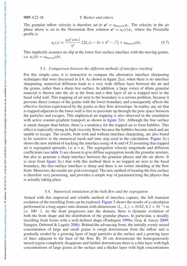
5.3. Comparison between the different methods of interface trackingFor this simple case, it is instructive to compare the alternative interface sharpeningtechniques that were discussed in § 4. As shown in figure 2(a), when there is no interfacesharpening, numerical diffusion leads to a very wide diffuse layer between the air andthe grains, rather than a sharp free surface. In addition, a large vortex of dilute granularmaterial is thrown into the air at the front and a thin layer of air is trapped next to thebasal solid wall. This trapping of air next to the boundary is a serious problem, because itprevents direct contact of the grains with the lower boundary and consequently affects theeffective friction experienced by the grains as they flow downslope. In reality, any air thatis trapped adjacent to the lower wall is free to percolate up through the pore space betweenthe particles and escapes. This unphysical air trapping is also observed in the simulationwith active counter-gradient transport as shown in figure 2(b). Although the free surfaceis much sharper than before, there is a tendency for the trapped air to form bubbles. Thiseffect is especially strong in high viscosity flows because the bubbles become stuck and areunable to escape. The results, both with and without interface sharpening, are also foundto be sensitive to the numerical mesh and time step used in the calculation. Figure 2(c)shows the new method of tracking the interface using (4.4) and (4.5) assuming that trappedair is segregated upwards, i.e. e = ez. The segregation velocity magnitude and diffusioncoefficients (see table 3) are chosen to give diffuse segregation inside the granular mixture,but also to generate a sharp interface between the granular phases and the air above. Itis clear from figure 2(c) that with this method there is no trapped air next to the basalboundary, the free-surface interface is sharp and there is no vortex shedding at the flowfront. Moreover, the results are grid converged. The new method of treating the free surfaceis therefore very promising, and provides a simple way of parameterizing the physics thatis actually taking place.
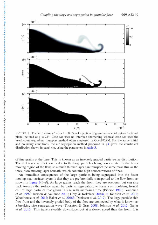
5.4. Numerical simulation of the bulk flow and the segregationArmed with this improved and reliable method of interface capture, the full transientevolution of the travelling front can be explored. Figure 3 shows the results of a calculationperformed in a long aspect ratio domain with dimensions (Lx ,Lz) = (0.62, 6.2 × 10⁻³) mi.e. 100 : 1. As the front progresses into the domain, there is dynamic evolution ofboth the front shape and the distribution of the granular phases. In particular, a steadilytravelling front forms with a well-defined shape (Pouliquen 1999a; Gray & Ancey 2009;Saingier, Deboeuf & Lagrée 2016). Behind the advancing front, the initially evenly mixedconcentration of large and small grains is swept downstream from the inflow and isgradually eroded by a growing layer of large particles at the surface and a growing layerof fines adjacent to the base of the flow. By 20 cm downstream the homogeneouslymixed region completely disappears and further downstream there is a thin layer with highconcentrations of large grains at the surface and a thicker layer with high concentrations
Coupling rheology and segregation in granular flows 909 A22-19
(×10–3)
(×10–3)
(×10–3)
(×10–3)
6
5
4
3
2
1
1.0
0.5
0
0
0
6
5
4
3
2
1
0 2 4 6 8 10 12 14 16 18 20
6
5
4
3
2
1
z(m)
z(m)
z(m)
x (m)
ϕa
(b)
(a)
(c)
FIGURE 2. The air fraction ϕa after t = 0.05 s of injection of granular material onto a frictionalplane inclined at ζ = 24◦. Case (a) uses no interface sharpening whereas case (b) uses theusual counter-gradient transport method often employed in OpenFOAM. For the same initialand boundary conditions, the air segregation method proposed in § 4 gives the constituentdistribution shown in panel (c), using the parameters in table 3.
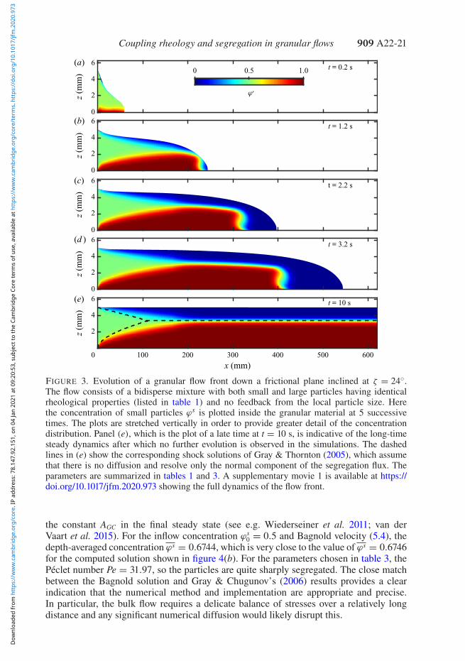
of fine grains at the base. This is known as an inversely graded particle-size distribution.The difference in thickness is due to the large particles being concentrated in the fastermoving region of the flow, so a much thinner layer can transport the same mass flux as thethick, slow moving layer beneath, which contains high concentrations of fines.
An immediate consequence of the large particles being segregated into the fastermoving near surface layers is that they are preferentially transported to the flow front, asshown in figure 3(b–d). As large grains reach the front, they are over-run, but can riseback towards the surface again by particle segregation, to form a recirculating frontalcell of large particles that grows in size with increasing time (Pierson 1986; Pouliquenet al. 1997; Iverson & Vallance 2001; Gray & Kokelaar 2010b, a; Johnson et al. 2012;Woodhouse et al. 2012; Baker et al. 2016b; Denissen et al. 2019). The large particle richflow front and the inversely graded body of the flow are connected by what is known asa breaking size segregation wave (Thornton & Gray 2008; Johnson et al. 2012; Gajjaret al. 2016). This travels steadily downslope, but at a slower speed than the front. It is
this wave that segregates the large slow moving particles, close to the base of the flow,up into faster moving regions allowing them to be recirculated, and conversely, allows fastmoving small grains to percolate down into slower moving basal layers. The breakingwave shown here includes the effects of diffusion as well as segregation for the firsttime. Eventually the flow front and the breaking size segregation wave propagate out ofthe domain, to leave the approximately steady uniform flow shown in figure 3(e). Forcomparison, Gray & Thornton’s (2005) concentration shock solution (see appendix A) isalso plotted in figure 3(e) using the Bagnold velocity profile (5.4). For an inflow smallparticle concentration ϕs
0 = 0.5 this accurately predicts the position of the centre of thefinal steady-state height of the inversely graded layer, with the large particles occupyinga thinner faster moving region than the fines. However, the solution neglects diffusion inboth the downslope and slope normal directions, and only resolves the segregation flux inthe slope normal direction, so it does not capture the precise point at which the solutionreaches steady state.
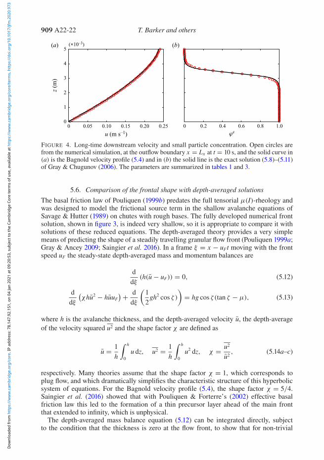
5.5. Comparison with steady uniform solutions for the bulk flow and the segregationFigure 4(a) shows excellent agreement between the computed two-dimensional steadyuniform flow solution for the downslope velocity u and the Bagnold velocity profile (5.4).The only slight difference occurs near the free surface, where the weight of the column ofair above produces the largest relative change in the pressure within the granular material.With the μ(I)-rheology, this changes the balances in the inertial number and hence thecomputed velocity profile. For steady uniform flows, Gray & Chugunov (2006) derivedan exact solution for the small particle concentration, assuming that the segregation anddiffusion rates were constant. This solution takes the form
ϕs = 11 + AGC exp(Pe z)
, (5.8)
where AGC is a constant and Pe is the Péclet number for segregation. Note that in thissolution the z-coordinate has been non-dimensionalized using the scaling z = hz, whereh is the slope normal flow depth. In terms of the dimensional segregation and diffusionrates, given in table 3, the Péclet number is defined as
Pe = fsl h cos ζDsl
, (5.9)
where the factor cos ζ arises from the fact that the segregation is inclined at an angle ζto the slope normal z-axis, i.e. ez · g/|g| = − cos ζ . The constant AGC alters the positionof the transition between large and small particles in the solution. If the depth-averagedconcentration is equal to
ϕs = 1h
∫ h
0ϕ(z) dz =
∫ 1
0ϕ(z) dz, (5.10)
then
AGC = exp(−Peϕs)− exp(−Pe)1 − exp(−Peϕs)
. (5.11)
The depth-averaged flux of small particles is the same at all downstream positions atsteady state. It follows that the upstream inflow conditions can be used to determine
Coupling rheology and segregation in granular flows 909 A22-21
z (m
m)
z (m
m)
z (m
m)
z (m
m)
z (m
m)
x (mm)
t = 0.2 s
t = 1.2 s
t = 2.2 s
t = 3.2 s
t = 10 s
ϕs
0
2
4
6
2
0
4
6
2
0
4
6
2
0
4
6
2
0
4
60 0.5 1.0
100 200 300 400 500 600
(e)
(b)
(a)
(c)
(d )
FIGURE 3. Evolution of a granular flow front down a frictional plane inclined at ζ = 24◦.The flow consists of a bidisperse mixture with both small and large particles having identicalrheological properties (listed in table 1) and no feedback from the local particle size. Herethe concentration of small particles ϕs is plotted inside the granular material at 5 successivetimes. The plots are stretched vertically in order to provide greater detail of the concentrationdistribution. Panel (e), which is the plot of a late time at t = 10 s, is indicative of the long-timesteady dynamics after which no further evolution is observed in the simulations. The dashedlines in (e) show the corresponding shock solutions of Gray & Thornton (2005), which assumethat there is no diffusion and resolve only the normal component of the segregation flux. Theparameters are summarized in tables 1 and 3. A supplementary movie 1 is available at https://doi.org/10.1017/jfm.2020.973 showing the full dynamics of the flow front.
the constant AGC in the final steady state (see e.g. Wiederseiner et al. 2011; van derVaart et al. 2015). For the inflow concentration ϕs
0 = 0.5 and Bagnold velocity (5.4), thedepth-averaged concentration ϕs = 0.6744, which is very close to the value of ϕs = 0.6746for the computed solution shown in figure 4(b). For the parameters chosen in table 3, thePéclet number Pe = 31.97, so the particles are quite sharply segregated. The close matchbetween the Bagnold solution and Gray & Chugunov’s (2006) results provides a clearindication that the numerical method and implementation are appropriate and precise.In particular, the bulk flow requires a delicate balance of stresses over a relatively longdistance and any significant numerical diffusion would likely disrupt this.
FIGURE 4. Long-time downstream velocity and small particle concentration. Open circles arefrom the numerical simulation, at the outflow boundary x = Lx at t = 10 s, and the solid curve in(a) is the Bagnold velocity profile (5.4) and in (b) the solid line is the exact solution (5.8)–(5.11)of Gray & Chugunov (2006). The parameters are summarized in tables 1 and 3.
5.6. Comparison of the frontal shape with depth-averaged solutionsThe basal friction law of Pouliquen (1999b) predates the full tensorial μ(I)-rheology andwas designed to model the frictional source term in the shallow avalanche equations ofSavage & Hutter (1989) on chutes with rough bases. The fully developed numerical frontsolution, shown in figure 3, is indeed very shallow, so it is appropriate to compare it withsolutions of these reduced equations. The depth-averaged theory provides a very simplemeans of predicting the shape of a steadily travelling granular flow front (Pouliquen 1999a;Gray & Ancey 2009; Saingier et al. 2016). In a frame ξ = x − uFt moving with the frontspeed uF the steady-state depth-averaged mass and momentum balances are
ddξ(h(u − uF)) = 0, (5.12)
ddξ
(χhu2 − huuF
) + ddξ
(12
gh2 cos ζ ))
= hg cos ζ(tan ζ − μ), (5.13)
where h is the avalanche thickness, and the depth-averaged velocity u, the depth-averageof the velocity squared u2 and the shape factor χ are defined as
u = 1h
∫ h
0u dz, u2 = 1
h
∫ h
0u2 dz, χ = u2
u2, (5.14a–c)
respectively. Many theories assume that the shape factor χ = 1, which corresponds toplug flow, and which dramatically simplifies the characteristic structure of this hyperbolicsystem of equations. For the Bagnold velocity profile (5.4), the shape factor χ = 5/4.Saingier et al. (2016) showed that with Pouliquen & Forterre’s (2002) effective basalfriction law this led to the formation of a thin precursor layer ahead of the main frontthat extended to infinity, which is unphysical.
The depth-averaged mass balance equation (5.12) can be integrated directly, subjectto the condition that the thickness is zero at the flow front, to show that for non-trivial
Coupling rheology and segregation in granular flows 909 A22-23
solutions the depth-averaged velocity is equal to the front speed, i.e.
u = uF, (5.15)
everywhere in the flow. Far upstream the flow is steady and uniform. The front speed cantherefore be determined by integrating the Bagnold solution (5.4) through the avalanchedepth to show that
uF = u∞ = 2Iζ5d
√Φg cos ζ h3/2
∞ , (5.16)
where h∞ and u∞ are the steady uniform thickness and downslope velocity far upstream.Expanding (5.13), dividing through by hg cos ζ and using (5.15) yields an ordinarydifferential equation (ODE) for the flow thickness[
(χ − 1)Fr2∞
h∞h
+ 1]
dhdξ
= tan ζ − μ, (5.17)
where Fr∞ is the Froude number far upstream, i.e.
Fr∞ = u∞√gh∞ cos ζ
. (5.18)
In order to solve the ODE (5.17) it is necessary to convert the new friction law (2.8) into aneffective basal friction law. This is done by assuming that Bagnold flow holds everywherein the flow and hence the depth-averaged downslope velocity u satisfies
u = 2I5d
√Φg cos ζ h3/2. (5.19)
Since, the depth-averaged velocity is the same as the front velocity (5.15) everywhere inthe flow, (5.16) and (5.19) can be equated to determine the inertial number
I(ξ) = Iζ
(h∞
h(ξ)
)3/2
, (5.20)
at a general position ξ . Substituting this expression into the high-I branch of the full μ(I)curve (2.8) gives the regularized depth-averaged basal friction
μ(h) =μsI0h3/2 + μdIζh3/2
∞ + μ∞I2ζ
(h∞√
h
)3
I0h3/2 + Iζh3/2∞
. (5.21)
The significance of this expression is made clear by taking the limit as h → 0. Unlikefor the previous expression for μ, in which μ∞ = 0, the friction now tends to infinityfor vanishingly thin layers. This means that the ODE (5.17) naturally predicts an infiniteslope and therefore the front always pins to the boundary and this system is guaranteed topreclude infinite precursor layers.
The front shape predicted by this newly derived regularized depth-averaged formulationis compared with the full two-dimensional numerics in figure 5. In order to guaranteethat the full solution does indeed correspond to a steady travelling front, the simulationis continued from t = 4 s in a moving frame. This change is applied simply by shifting
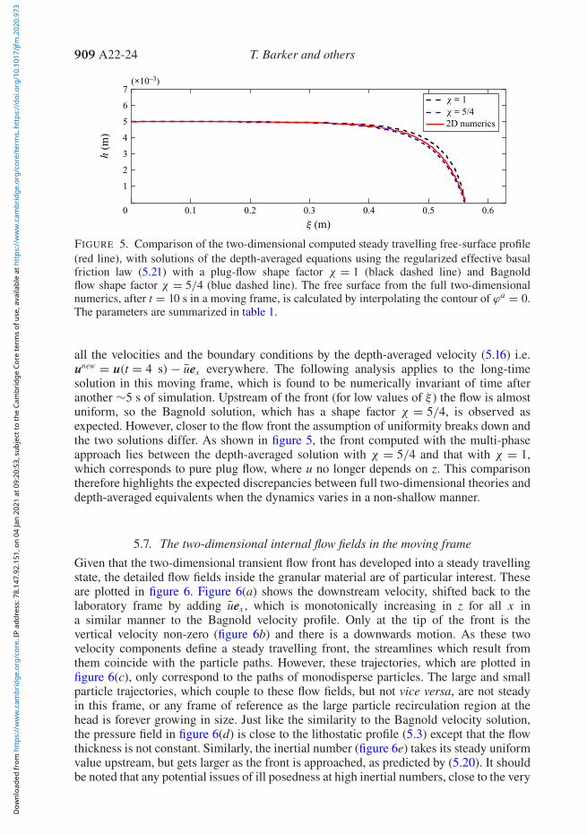
FIGURE 5. Comparison of the two-dimensional computed steady travelling free-surface profile(red line), with solutions of the depth-averaged equations using the regularized effective basalfriction law (5.21) with a plug-flow shape factor χ = 1 (black dashed line) and Bagnoldflow shape factor χ = 5/4 (blue dashed line). The free surface from the full two-dimensionalnumerics, after t = 10 s in a moving frame, is calculated by interpolating the contour of ϕa = 0.The parameters are summarized in table 1.
all the velocities and the boundary conditions by the depth-averaged velocity (5.16) i.e.unew = u(t = 4 s)− uex everywhere. The following analysis applies to the long-timesolution in this moving frame, which is found to be numerically invariant of time afteranother ∼5 s of simulation. Upstream of the front (for low values of ξ ) the flow is almostuniform, so the Bagnold solution, which has a shape factor χ = 5/4, is observed asexpected. However, closer to the flow front the assumption of uniformity breaks down andthe two solutions differ. As shown in figure 5, the front computed with the multi-phaseapproach lies between the depth-averaged solution with χ = 5/4 and that with χ = 1,which corresponds to pure plug flow, where u no longer depends on z. This comparisontherefore highlights the expected discrepancies between full two-dimensional theories anddepth-averaged equivalents when the dynamics varies in a non-shallow manner.
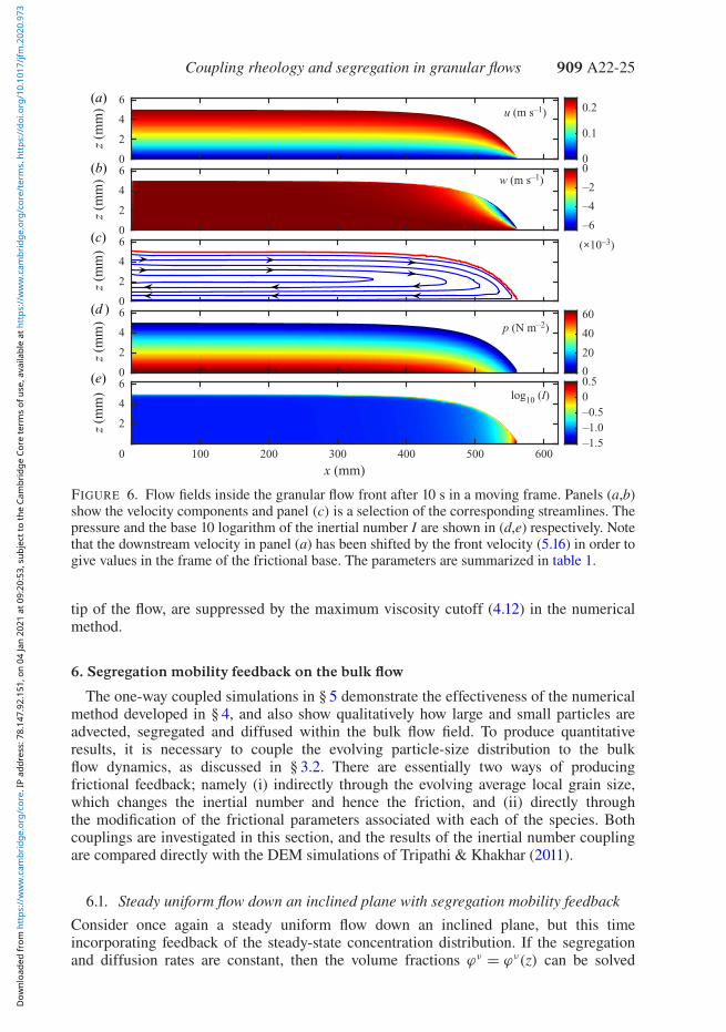
5.7. The two-dimensional internal flow fields in the moving frameGiven that the two-dimensional transient flow front has developed into a steady travellingstate, the detailed flow fields inside the granular material are of particular interest. Theseare plotted in figure 6. Figure 6(a) shows the downstream velocity, shifted back to thelaboratory frame by adding uex , which is monotonically increasing in z for all x ina similar manner to the Bagnold velocity profile. Only at the tip of the front is thevertical velocity non-zero (figure 6b) and there is a downwards motion. As these twovelocity components define a steady travelling front, the streamlines which result fromthem coincide with the particle paths. However, these trajectories, which are plotted infigure 6(c), only correspond to the paths of monodisperse particles. The large and smallparticle trajectories, which couple to these flow fields, but not vice versa, are not steadyin this frame, or any frame of reference as the large particle recirculation region at thehead is forever growing in size. Just like the similarity to the Bagnold velocity solution,the pressure field in figure 6(d) is close to the lithostatic profile (5.3) except that the flowthickness is not constant. Similarly, the inertial number (figure 6e) takes its steady uniformvalue upstream, but gets larger as the front is approached, as predicted by (5.20). It shouldbe noted that any potential issues of ill posedness at high inertial numbers, close to the very
Coupling rheology and segregation in granular flows 909 A22-25
0
2
4
6
0
0.1
0.2
0
2
4
6
–6
–4
–2
0
(×10–3)
0
2
4
6
0
2
4
6
0
20
40
60
0 100 200 300 400 500 600
2
4
6
–1.5–1.0–0.500.5
x (mm)
z (m
m)
z (m
m)
z (m
m)
z (m
m)
z (m
m) u (m s–1)
w (m s–1)
p (N m–2)
log10 (I)(e)
(b)
(a)
(c)
(d )
FIGURE 6. Flow fields inside the granular flow front after 10 s in a moving frame. Panels (a,b)show the velocity components and panel (c) is a selection of the corresponding streamlines. Thepressure and the base 10 logarithm of the inertial number I are shown in (d,e) respectively. Notethat the downstream velocity in panel (a) has been shifted by the front velocity (5.16) in order togive values in the frame of the frictional base. The parameters are summarized in table 1.
tip of the flow, are suppressed by the maximum viscosity cutoff (4.12) in the numericalmethod.
6. Segregation mobility feedback on the bulk flow
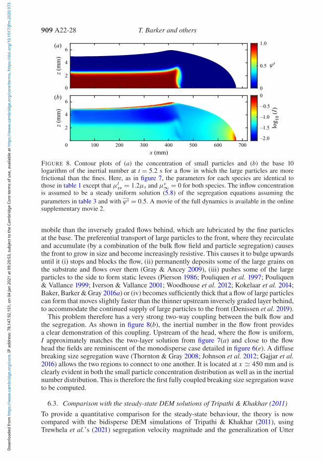
The one-way coupled simulations in § 5 demonstrate the effectiveness of the numericalmethod developed in § 4, and also show qualitatively how large and small particles areadvected, segregated and diffused within the bulk flow field. To produce quantitativeresults, it is necessary to couple the evolving particle-size distribution to the bulkflow dynamics, as discussed in § 3.2. There are essentially two ways of producingfrictional feedback; namely (i) indirectly through the evolving average local grain size,which changes the inertial number and hence the friction, and (ii) directly throughthe modification of the frictional parameters associated with each of the species. Bothcouplings are investigated in this section, and the results of the inertial number couplingare compared directly with the DEM simulations of Tripathi & Khakhar (2011).
6.1. Steady uniform flow down an inclined plane with segregation mobility feedbackConsider once again a steady uniform flow down an inclined plane, but this timeincorporating feedback of the steady-state concentration distribution. If the segregationand diffusion rates are constant, then the volume fractions ϕν = ϕν(z) can be solved
for with the polydisperse theory in § 2.2, completely independently of the bulk flow.These concentrations will therefore be assumed to be known in what follows. The normalcomponent of the momentum balance then implies that the pressure is lithostatic (5.3).The only difference to the classical Bagnold solution (Silbert et al. 2001; GDR MiDi2004; Gray & Edwards 2014) is that, with the volume fraction weighted friction (3.3), thedownslope momentum balance reduces to∑
∀νϕνμν(I) = tan ζ, (6.1)
whereμν is the friction law for constituent ν. For the purposes of illustration, let us assumethat each phase satisfies the classical μ(I) friction law, which is of the form
μν = μνs + μνd − μνs
I0/I + 1, (6.2)
where I0 is assumed to be the same for all the phases. Substituting (6.2) into (6.1) andsolving for the inertial number, it follows that
I = I0
(tan ζ − μs
μd − tan ζ
), (6.3)
where μs and μd are now the volume fraction weighted averages that are depth dependent
μs(z) =∑∀νϕν(z)μνs , μd(z) =
∑∀νϕν(z)μνd. (6.4a,b)
Importantly, (6.3) shows that, if there are frictional differences between the particles, thenthe inertial number is dependent on the normal coordinate z rather than being equal tothe constant Iζ defined in (5.5). Using the definition of the generalized inertial number forpolydisperse systems (3.2) and assuming steady uniform flow, it follows that the ODE forthe velocity profile is
dudz
= I0
d
√Φg cos ζ (h − z)1/2
(tan ζ − μs
μd − tan ζ
)(6.5)
where d is the local average particle size, which is also depth dependent
d(z) =∑∀νϕν(z)dν. (6.6)
This averaged particle-size dependence is important, because even if the particles have thesame shape and the same effective frictional properties, the velocity profile will no longerbe the classical Bagnold solution (5.4), but will depend on the local changes in particlesize.
Figure 7 shows a specific example of the qualitative types of solution that are generatedfor a bidisperse mixture of large and small particles. The solutions assume Gray &Chugunov’s (2006) exact solution for the concentration profile (5.8)–(5.11) using thesame constant segregation velocity magnitude fsl, constant diffusivity Dsl, flow depth has in table 3, as well as the same slope angle ζ = 24◦. The only difference is that thedepth-averaged concentration ϕs is chosen to be equal to 50 % in order to produce flowing
Coupling rheology and segregation in granular flows 909 A22-27
I u (m s–1)0.060.040.02
00 0.1 0.2
1
2z (m
) 3
4
5(×10–3) (b)(a)
FIGURE 7. Exact solutions for (a) the inertial number and (b) the downstream velocity for abidisperse mixture of large and small particles (black lines) on a slope inclined at ζ = 24◦ tothe horizontal. The solutions assume a small particle concentration profile given by Gray &Chugunov’s (2006) exact solution in (5.8)–(5.11), with ϕs = 0.5 and using the parameters intable 3. Here, all bulk flow parameters are identical to those in table 1 except that the largeparticles have μl
s = 1.2μs and μν∞ = 0 for both phases. The dashed lines indicate uniformconcentration solutions with red corresponding to pure large, blue corresponding to pure smallparticles and green being the solution for a mixture with ϕs = 0.5 everywhere.
layers of large and small particles that are the same depth. For consistency with theassumed friction law (6.2), μν∞ = 0 for both the large and small particles. All the otherparameters are the same for both species, and identical to those given in table 1, exceptthat μl
s = 1.2μs. This small change is sufficient to make the inertial number (6.3) depthdependent, as shown in figure 7(a). The increase in μl
s for the large particles decreasesthe inertial number in the near surface regions, where the large particles are located.Integrating the ODE (6.5) through the flow depth, subject to the no slip condition at thebase, gives the velocity profile in figure 7(b). The solution lies between the velocity profilesfor pure large and for pure small particles, and closely follows the small particle velocityprofile in the lower part of the flow, where the small particles are concentrated. In the upperpart of the flow it rapidly transitions onto a curve that is parallel to that of the pure largeparticles, but they attain a much higher speed than if there were no small particles in theflow. Or indeed, if the particles were evenly mixed throughout the column with ϕs = 1/2everywhere. The small particles therefore provide an important lubricating mechanismthat can significantly increase flow speeds and the overall run-out (Kokelaar et al. 2014).
6.2. Formation of a large rich bulbous flow front on an inclined planeGiven the steady solution in § 6.1, it is also interesting to consider the transient behaviourof a granular flow front when the large particles are more frictional than the fines.Analogously to the DEM study of Denissen et al. (2019), the solution detailed in figure 7 isused as the boundary condition at the inlet wall x = 0, so that material entering the domainis already stratified and well developed. All parameters are the same as those in § 6.1. Asshown in figure 8(a), the two-dimensional transient dynamics generates a bulbous head oflarge particles in front of an approximately uniform thickness upstream flow. This bulgingof the surface differs from the monotonically decreasing free-surface shape, observedwhen there is no feedback of the segregation on the bulk, as shown in § 5 and figures 3–6.The fundamental cause of this effect is that pure regions of large particles are much less
FIGURE 8. Contour plots of (a) the concentration of small particles and (b) the base 10logarithm of the inertial number at t = 5.2 s for a flow in which the large particles are morefrictional than the fines. Here, as in figure 7, the parameters for each species are identical tothose in table 1 except that μl
s∗ = 1.2μs and μν∞ = 0 for both species. The inflow concentrationis assumed to be a steady uniform solution (5.8) of the segregation equations assuming theparameters in table 3 and with ϕs = 0.5. A movie of the full dynamics is available in the onlinesupplementary movie 2.
mobile than the inversely graded flows behind, which are lubricated by the fine particlesat the base. The preferential transport of large particles to the front, where they recirculateand accumulate (by a combination of the bulk flow field and particle segregation) causesthe front to grow in size and become increasingly resistive. This causes it to bulge upwardsuntil it (i) stops and blocks the flow, (ii) permanently deposits some of the large grains onthe substrate and flows over them (Gray & Ancey 2009), (iii) pushes some of the largeparticles to the side to form static levees (Pierson 1986; Pouliquen et al. 1997; Pouliquen& Vallance 1999; Iverson & Vallance 2001; Woodhouse et al. 2012; Kokelaar et al. 2014;Baker, Barker & Gray 2016a) or (iv) becomes sufficiently thick that a flow of large particlescan form that moves slightly faster than the thinner upstream inversely graded layer behind,to accommodate the continued supply of large particles to the front (Denissen et al. 2019).
This problem therefore has a very strong two-way coupling between the bulk flow andthe segregation. As shown in figure 8(b), the inertial number in the flow front providesa clear demonstration of this coupling. Upstream of the head, where the flow is uniform,I approximately matches the two-layer solution from figure 7(a) and close to the flowhead the fields are reminiscent of the monodisperse case detailed in figure 6(e). A diffusebreaking size segregation wave (Thornton & Gray 2008; Johnson et al. 2012; Gajjar et al.2016) allows the two regions to connect to one another. It is located at x 450 mm and isclearly evident in both the small particle concentration distribution as well as in the inertialnumber distribution. This is therefore the first fully coupled breaking size segregation waveto be computed.
6.3. Comparison with the steady-state DEM solutions of Tripathi & Khakhar (2011)To provide a quantitative comparison for the steady-state behaviour, the theory is nowcompared with the bidisperse DEM simulations of Tripathi & Khakhar (2011), usingTrewhela et al.’s (2021) segregation velocity magnitude and the generalization of Utter
Coupling rheology and segregation in granular flows 909 A22-29
& Behringer’s (2004) diffusivity to bidisperse systems (rather than prescribed rates). Theresults shown in Tripathi & Khakhar’s (2011) figure 9 correspond to flow down a planeinclined at an angle ζ = 25◦, in which the large particle diameter is one and a half timesthe small grain diameter, i.e. dl = 1.5ds. The results are presented in non-dimensionalform, where the length, time and velocity scalings
z = dsz, h = dsh, t =√
ds/g t, u =√
gdsu, (6.7a–d)
are based on the small particle diameter ds and gravity g. The layer depth h is assumed tobe 30ds. The simulations are performed in a three-dimensional cell that is periodic in thedown and cross-slope directions, and has a fixed bed that is made rough with particlesof diameter 1.2ds. The down and cross-slope dimensions are 20ds × 20ds. Figure 9shows Tripathi & Khakhar’s (2011) computed small particle concentration and downslopevelocity for five different depth-averaged concentrations, ranging from pure small to purelarge.
For comparison, the bidisperse small particle concentration equation (2.19) is solved atsteady state, assuming the functional forms (3.7) and (3.9) for the segregation velocitymagnitude and diffusivity, i.e.
fsl = 2Bρ∗g‖D‖d2
Cρ∗gd + p
[(R − 1)+ Eϕl(R − 1)2
], Dsl = 2A‖D‖d2, (6.8a,b)
where A, B, C and E are non-dimensional constants and γ has been replaced by itsequivalent strain-rate invariant, i.e. 2‖D‖. Assuming that the downslope velocity andthe small particle concentration are purely functions of the slope normal coordinate z,(2.19) can be integrated once with respect to z. Applying the no flux boundary condition(2.17) at the surface and/or base of the flow, the ‖D‖d2 dependence in the segregation anddiffusive terms cancels out. As a result the final steady-state ODE for the concentration isindependent of the shear rate, uncoupling it from the downslope momentum balance.
The non-dimensional parameter C is primarily introduced to remove the pressuresingularity at the free surface, and its measured value of C = 0.2712 makes very littledifference to the shape of the concentration profile (Trewhela et al. 2021). If instead C isassumed to be zero, and the pressure is lithostatic (5.3), then the intrinsic grain density ρ∗,gravity g and the slope angle ζ cancel out, leaving a non-dimensional steady-state ODEfor the concentration
dϕs
dz= −B(R − 1)ϕsϕl(1 + Eϕl(R − 1))
ΦA(h − z), (6.9)
which is dependent purely on the grain-size ratio R. This is separable, and can be integrated(Trewhela et al. 2021) to give the exact solution
z = h − K(1 − ϕs)−λ1(1 + E(1 − ϕs)(R − 1))λ2(ϕs)λ3, (6.10)
where K is a constant of integration and the coefficients λ1, λ2 and λ3 are
λ1 = ΦAB(R − 1)
, λ2 = ΦAEB(1 + E(R − 1))
, λ3 = ΦAB(R − 1)(1 + E(R − 1))
.
(6.11a–c)For a given depth-averaged small particle concentration ϕs the constant of integrationK can be determined iteratively. Figure 9(a) shows the comparison between these exact
FIGURE 9. Comparison of Tripathi & Khakhar’s (2011) DEM simulations (markers) withtheory (lines) for (a) the small particle concentration ϕs and (b) the downslope velocity uat different depth-averaged small particle concentration ϕs = 0, 30, 50, 70 and 100 %. Thenon-dimensional segregation constants are summarized in table 2 and the velocity is calculatedusing Tripathi & Khakhar’s (2011) values of μs = tan(20.16◦) and μd = tan(37.65◦), whileI0 = 0.5106 is used to fit the steady-state 100 % small particle velocity profile.
solutions and the DEM simulations of Tripathi & Khakhar (2011) for depth-averagedconcentrations ϕs = 0, 30, 50, 70 and 100 %. The agreement in the monodisperse limitsof ϕs = 0 and 100 % are guaranteed. There is also very good agreement at ϕs = 50 %and 70 % using exactly the same non-dimensional constants A, B and E determinedexperimentally by Trewhela et al. (2021) and summarized in table 2. The theory thereforematches the stronger segregation at the surface than the base of the flow, as well as
Coupling rheology and segregation in granular flows 909 A22-31
the gradient of the concentration profiles, without the need for any fitting parameters.This is strong evidence that Trewhela et al.’s (2021) theory captures the essence of thesegregation process. It also contrasts with Gray & Chugunov’s (2006) solution, where theratio of segregation to diffusion is uniform with depth. The agreement between Trewhelaet al.’s (2021) theory and Tripathi & Khakhar’s (2011) DEM simulations is not as goodat ϕs = 30 %. The DEM results at ϕs = 30 % look slightly odd, with a layer of almostpure small particles at the base of the cell and a much more diffuse profile higher up.It is therefore possible that, in this particular case, Tripathi & Khakhar’s (2011) DEMsimulations have not fully reached steady state.
Figure 17 of Tripathi & Khakhar (2011) suggests that the friction in both theirmonodisperse and bidisperse systems was closely approximated by the classical μ(I)law (2.7), using the generalized inertial number (3.2) with a local average grain size d.To leading order, therefore, the macroscopic friction coefficients μs and μd, as well atthe non-dimensional constant I0 are the same for the large and small particles. Tripathi& Khakhar (2011) suggested that a good overall fit to the data was provided by μs =tan(20.16◦), μd = tan(37.65◦) and I0 = 0.434. These values are, however, not good forthe particular set of simulations shown in Tripathi & Khakhar’s (2011) figure 9, andreproduced here in figure 9. To select a better fit, the Bagnold solution (5.4) has beennon-dimensionalized using the scalings (6.7a–d) to give
uBagnold = 23 Iζ
√Φ cos ζ
(h3/2 − (h − z)3/2
)(6.12)
and then fitted to the small particle velocity DEM data using a least squares fit. Thisdetermines the value of Iζ , which for the classical friction law (2.7) of Jop et al. (2006) isdefined as
Iζ = I0
(tan ζ − μs
μs − tan ζ
). (6.13)
The values of μs, μd and I0 can therefore be modified, while still fitting the data, providedthe same value of Iζ is obtained. There are an infinite number of combinations thatwill do this. This paper therefore assumes that the values of μs and μd are the same asTripathi & Khakhar (2011), but that I0 = 0.5106. To solve for the velocity profiles at otherconcentrations it is necessary solve the ODE (6.5) in non-dimensional form, i.e.
dudz
= Iζ√Φ cos ζ
(ϕs + Rϕl)(h − z)1/2, (6.14)
subject to a no-slip boundary condition at the base. In the ODE (6.14) the small particleconcentration ϕs = 1 − ϕl is given by Trewhela et al.’s (2021) exact solution (6.10). Thesolutions are shown in figure 9(b). The 100 % small particle solution agrees extremelywell with the Bagnold solution (6.12), which is not too surprising as the parameters μs, μdand I0 have been chosen specifically to match this curve. The monodisperse large particlesolution also has a Bagnold-like velocity profile, but the magnitude of the velocities areslightly underpredicted. In principle, the monodisperse small particle solution shouldbe a factor R larger than the large particle solution. The fact that they are not, is anindication of either (i) the level of noise in Tripathi & Khakhar’s (2011) system, or(ii) the basal roughness not scaling with the size of flowing particles (i.e. non-local effects).Since the deviations of the intermediate solutions from the DEM data are of a similarorder of magnitude, it is probably unwise to read too much into the precise comparisons.The predicted velocity profiles at intermediate concentrations monotonically decrease in
magnitude as the small particle content decreases. This is broadly speaking what the DEMdata show; however, the case ϕs = 30 % the DEM solution is again anomalous, beingbelow the case of pure large particles (Tripathi & Khakhar 2011). To be sure that this is realbehaviour, rather than an anomaly, more precise DEM solutions are required that averageover significantly more than the approximately 4000–12 000 particles used by Tripathi &Khakhar (2011).
7. Fully coupled rotating drum simulations
Particle segregation in non-circular rotating drums provides an ideal test case forthe two-way coupled model, as the particles strongly segregate and diffuse in the nearsurface liquid-like avalanche, but not in the solid-like rotating body beneath. Computingthe bulk flow field in a rotating drum is still a significant challenge. Indeed, recentsegregation simulations in a circular rotating drum (Schlick et al. 2015) have prescribed thesteady-state incompressible bulk velocity field based on fits to DEM simulations; a processthat inherently relies on the steady-state nature and simple geometry of the circular drum.More complex models that do use a continuum approach to calculate the bulk flow in acircular drum (e.g. Liu, Gonzalez & Wassgren 2018, 2019), do so with rate-independentelasto-plastic constitutive laws which are prone to ill posedness (Schaeffer 1987). Thispaper goes considerably further, by using the partially regularized μ(I)-rheology and therecent segregation model of Trewhela et al. (2021) to simultaneously compute the fullytwo-way coupled bulk flow, segregation and diffusion in a square rotating drum.
7.1. Modelling the bulk flow, segregation and diffusion in a square rotating drumIt is useful to have two coordinate systems to simulate the flow in the drum. The firstis a rectangular Cartesian coordinate system Oxz that is fixed and centred at the axis ofrotation of the drum, which lies at the centre of the square. The z axis is aligned with thegravitational acceleration g, but points upwards in the opposite sense. A second coordinatesystem OXZ is inclined at an angle θ to Oxz and rotates with the drum. The axes are alignedwith the drum walls, so the drum lies in the region −L ≤ X ≤ L, −L ≤ Z ≤ L, where 2Lis the length of the walls. Initially, the OXZ axes coincide with Oxz and the concentrationsof excess air, small particles and large particles are
(ϕa, ϕs, ϕl)∣∣t=0 =
⎧⎪⎨⎪⎩(1, 0, 0), for H < Z ≤ L,(
0,12,
12
), for − L ≤ Z ≤ H,
(7.1)
where L = 0.1 m and H = 0.04 m, implying a 70 % fill fraction with a 50 : 50 mix oflarge and small particles of diameters dl = 2 mm and ds = 1 mm, respectively. A fillfraction above 50 % is chosen so that an undisturbed core forms in the centre of the drum,consisting of material which never enters the avalanche (see e.g. Gray & Hutter 1997; Gray2001). All the material is initially assumed to be in solid-body rotation
u0 = Ωrθ , (7.2)
whereΩ is the rotation rate, the radial coordinate r = √x2 + z2 and θ is the azimuthal unit
vector. A constant rotation rate of Ω = −π/5 rad s−1 is specified, with the negative signdenoting clockwise rotation. This corresponds to one full revolution every 10 s, placingthe flow at the upper end of rolling flow (Henein, Brimacombe & Watkinson 1983;
Coupling rheology and segregation in granular flows 909 A22-33
μs = tan(20.16◦), μd = tan(37.65◦), μ∞ = 0.03,I0 = 0.5106, α = 1.9, I1 = 0.01886dl = 2 mm ds = 1 mm R = 2,
fal = fas = 1 m s−1, Dal = Das = 0 m2 s−1, e = −g/|g| = k.
TABLE 4. The fully coupled rotating drum simulations are performed with Barker & Gray’s(2017) partially regularized friction law with parameters that match the steady-state DEMsimulations of Tripathi & Khakhar (2011) shown in figure 9. The value of μ∞ is chosen to ensurethat the equations remain well-posed up to a maximum inertial number Imax = 16.20, while I1 isthe minimum well-posed inertial number in the unregularized law. To handle the evolving freesurface, the excess air segregates with a constant rate fal = fas from the large and small particlesand does not diffuse with them. The air phase is assumed to segregate upwards in the directionof the unit vector k along the z-axis, which this time is aligned with gravity.
Ding et al. 2002; Yang et al. 2008). This is also known as the continuous, or thecontinuously avalanching, regime (Rajchenbach 1990; Gray 2001) as a quasi-steady-stateavalanche forms, with continuous erosion and deposition occurring with the solid rotatingbody of grains beneath. The frictional parameters are the same for the large and smallparticles, and the momentum coupling enters via the evolving local average particle sized in the generalized inertial number (3.2). The values of μs, μd and I0 are the same asthose used to fit the DEM simulations of Tripathi & Khakhar (2011) (see figure 9), and thetheory is partially regularized (Barker & Gray 2017) by introducing a creep state at lowinertial numbers and a linear friction regime at high inertial numbers. The values of allthe frictional parameters are summarized in table 4, together with the particle sizes,and the air segregation and diffusion rates. The segregation of the particles is performedusing the same non-dimensional constants A, B, C and E suggested by Trewhela et al.(2021) and summarized in table 2.
The velocity field u in the rotating frame is related to the velocity u in the fixedcoordinate system by the relation
u = u −Ωrθ . (7.3)
As the drum rotates the no-slip and no-penetration (no flux) conditions are enforced onthe drum walls, which implies that
u = 0, on X = ±L and Z = ±L. (7.4)
These conditions are mapped back to the fixed coordinate system and applied onthe moving mesh using OpenFOAM’s mesh-motion routines. The computations areperformed on a regular N × N mesh, with results presented for the finest resolution studiedof N = 200. The simulation runs for eight full revolutions.
7.2. Bulk velocity, pressure and inertial number in the square drumInitially the free surface is flat and the material is in solid-body rotation, see (7.1) and(7.2). The entire body of grains is therefore quasi-static in the moving frame, and the highviscosity cut-off (4.12) remains active until the free-surface inclination nears the static
at which point the material near the free surface fails and avalanches downslope. After theinitial failure and slump, a continuously avalanching regime rapidly establishes itself, asshown in figure 10 and the supplementary movies. There is a rapid liquid-like avalancheclose to the free surface and a solid-like quasi-static region beneath (figure 10a,b).The angle of the free surface remains close to the static value ζs, but the position of thefree surface subtly rises and falls as the finite volume of grains is incorporated into theconstantly changing intersections with the shape of the drum during each quarter turn.The flow therefore has a quasi-periodic pulsing behaviour, with peak surface velocities (atthe centre and surface of the flow) changing in time, e.g. the peak free-surface velocity isfaster at t = 80 s than at t = 78.75 s in figure 10(a,b). As shown in § 6.3, the variationsin velocity with the flow composition are subtle, and do not provide a strong feedback onthe bulk flow at this fill height. However, the experiments of Zuriguel et al. (2006) implythat for fill levels close to 50 % these subtle composition-dependent velocity changes cancause the formation of petal-like structures in the deposit, and so can be very important.
As the flow pulses, the surface avalanche becomes deeper directly beneath the regionwhere the peak velocities are attained. The avalanche depth also changes along its length,reaching a peak near its centre. Typically the main flow is confined to a layer with amaximum thickness of 1.6 cm, which gives the rapid free-surface flow a shallow aspectratio, consistent with the assumptions underpinning theoretical models for avalanches (e.g.Savage & Hutter 1989; Gray 2001; Gray & Edwards 2014). Close to the free surface thepressure is approximately lithostatic and is aligned with the free surface (figure 10c,d)as one might expect. However, lower down the pressure rises to much higher valuesand pulses as the overall volume of grains redistributes itself in the changing geometryof the walls that confine it. The base ten logarithm of the inertial number is shown infigure 10(e, f ) and also identifies the near surface region where the failure occurs. Theflow is in a creep state for I < I1 = 0.01886. This region lies significantly higher in theflow than the Newtonian viscous region, which is activated by the numerical regularization(4.12) at high viscosities. The dominant rheology in the simulation is therefore the granularrheology, which involves regions of both creep and dynamic motion.
For fill levels above approximately 55 % a solid core develops (Mounty 2007), withinwhich particles are simply rotated around with the drum and undergo a small amount ofcreep when they are closer to the free surface. The remaining grains pass through both thesolid-like and fluid-like regions. These particles are rotated around with the drum in thesolid-body region, until they approach the near surface layers when they begin to creepdownslope. As an individual particle is rotated further towards the free surface the creepbecomes progressively stronger, until finally it avalanches downslope in the liquid-likesurface avalanche. As more particles are entrained into this avalanche it becomes deeperand flows faster, so peak velocities are reached midway down the slope, after whichparticles are deposited from the base of the flow, and the avalanche thins and slows. Anindividual particle therefore accelerates downslope in the first half of the avalanche anddecelerates after the midway point, before being deposited into the slowly creeping body ofrotating grains beneath. Unlike a circular drum, where monodisperse particles form closedstreamlines, the changing geometry of the confining walls adds considerable complexity tothe problem. This is because the underlying particle trajectories become chaotic even formonodisperse flows (Hill et al. 1999; Ottino & Khakhar 2000). Particle-size segregation,however, introduces a strong organizational influence on the resulting patterns that form.
Coupling rheology and segregation in granular flows 909 A22-35
|u| (m s–1)
p[N m–2]
log10 (I )
t = 77.5 s t = 80 s
0 0.1 0.2 0.3
0 1 2 3(×103)
–4 –3 –2 –1 0 1
(c)(d )
(a)(b)
(e)( f )
FIGURE 10. Periodic motion of the bulk flow shown at t = 78.75 s (a,c,e) and t = 80 s(b,d, f ), for (a,b) velocity magnitude in the rotating frame (i.e. minus the solid body rotation),(c,d) pressure and (e, f ) base 10 logarithm of the inertial number I. The dashed lines in (e, f )indicate the height below which the high viscosity cutoff becomes active. The parametersused to compute the bulk flow, segregation and diffusion are summarized in tables 2 and 4.Supplementary movies 3–5 showing the full periodic solution are available in the onlinesupplementary movies.
7.3. The particle-size distribution in the square drumThe dynamics of the mixing and segregation process is shown in figure 11 and thesupplementary online movie. As the drum rotates up to the static angle of friction thereis no shear and hence no segregation or diffusion. However, as soon as the initial failureoccurs, and the avalanche flows downslope, the particles begin to segregate with the largeparticles rising to the free surface and the small particles percolating downwards. Thelinear shear rate dependence in (6.8a,b) ensures that both the segregation and diffusionare confined to the thin avalanching layer close to the free surface, with the additionalpressure dependence ensuring that segregation shuts off more rapidly than the diffusionwith increasing depth (Golick & Daniels 2009; Fry et al. 2018; Trewhela et al. 2021).This effect is compounded by the fact that particles near the free surface travel the longestdistance through the liquid-like avalanche, while those that are entrained at lower levelsmay move only a short distance before they are deposited back into the solid-like rotatingbody of grains beneath. As a result, after the first full rotation of the drum (at t = 10 s) theclearest segregation can be seen in the large particles that are able to rise to the surfaceand collect at the top of the flow before being deposited near the drum wall. The rest ofthe grains remain quite well mixed.
After approximately 3/4 of a drum revolution all the material that is able to pass throughthe surface avalanche has done so, and the material that is subsequently entrained is nolonger homogenously mixed. The large particles that were deposited next to the drumwall are rotated around and re-entrained into the avalanche right at the back of the flow,where the avalanche is thinnest. There is therefore no need for them to segregate towardsthe surface again, as they are naturally re-entrained on trajectories that pass through thesurface layers of the avalanche. The particles that lie closer to the drum core are naturallyentrained onto paths that take them through lower regions of the avalanche. They thereforeget another chance to segregate again each time they pass through the avalanche. Thisprocess can be seen slowly sharpening the segregation in the successive panels of figure 11.With increasing time, the large particle region adjacent to the drum wall thickens up andregions with high concentrations of small particles start to emerge, as the avalanche at thesurface becomes progressively more inversely graded. Complete separation of the largeand small grains does not occur, however, because of the diffusive remixing process in(2.19).
The combination of particle segregation and the rising and falling of the free-surfaceheight as the drum rotates leads to the spontaneous formation of three lobes with highconcentrations of small particles, that are oriented towards the corners of the drum.These lobes are interesting because they propagate around the drum faster than the drumrotates, with a period of approximately 7.5 s. The lobes are in qualitatively very goodagreement with the experiments of Hill et al. (1999), Ottino & Khakhar (2000) andMounty (2007), as shown in figure 12. The simulations also predict the formation of acentral core within which the concentration is almost unchanged from its initial value.This core forms a shape that is almost square and lies at an angle of 45◦ to the squaredrum walls, which is also qualitatively in agreement with the experiments of Hill et al.(1999), Ottino & Khakhar (2000) and Mounty (2007). However, the simulated centralcore is about half the diameter of that in experiment. The reason for this is that thesurface avalanche is much deeper in the simulations than in the experiments. This is notnecessarily a deficiency of the model. The experiments are performed in drums with anarrow gap between the sidewalls; as a result the avalanche is thinner and faster thanin a drum with a wide cross-section (Jop et al. 2005) and hence the central core islarger.
Coupling rheology and segregation in granular flows 909 A22-37
ϕs0 0.2 0.4 0.6 0.8 1.0
(b)(a) (c)
(e)(d) ( f )
(h)(g) (i)
(k)( j) (l)
FIGURE 11. Fully coupled simulation of a bidisperse granular mixture in a square rotating drumusing the parameters in tables 2 and 4, where the drum walls are of length 0.2 m: (a) plots ϕs at10 s and (b–l) correspond to a further 6.25 s of rotation, or 5/8 of a full revolution, up to 78.75 s.A movie 6 is available in the online supplementary movies.
One of the important consequences of the ‖D‖d2 dependence in the segregation velocitymagnitude and diffusivity in (6.8a,b) is that the time scale for segregation and diffusionto occur is proportional to h2/(γ d2). It therefore takes longer to segregate in a deeperavalanche, or with smaller average grain sizes. This makes direct comparison with the
FIGURE 12. (a) Computed particle-size distribution after 78.1 s and (b) a comparable patternformed in a rotating drum (Mounty 2007) with small white particles (75–150 μm) and large redparticles (400–500 μm).
experiments difficult, as the depth and velocity of the surface avalanche is stronglyinfluenced by sidewall friction. In principle, it is very easy to include the effect of sidewallfriction in the simulations. However, the numerical method requires sufficient grid pointsto be located in the surface avalanche. For a regular grid this requires higher resolutionthroughout the drum, which dramatically increases the time necessary to produce gridconverged results, and so this is not done here. Instead the grain sizes are made larger inorder to get the pattern to form in the rotating drum simulations in a comparable time scaleto that in the experiments.
The lobes do not appear to reach a quasi-periodic steady state, but have smallprotuberances that continue to evolve when tracking a particular lobe. This is also inaccordance with experimental observation, as a non-homogeneous initial distribution ofparticles can lead to lobes of different sizes, which appear to persist indefinitely. Figure 11also shows that over long periods of time the central core contracts towards the origin.This is due to the slow creep that occurs as the material in the solid-body region is rotatedthrough the near surface creeping zone, where both segregation and diffusion can act oververy long time scales. This creep can be minimized either by (i) introducing sidewallfriction or (ii) by using constitutive equations with a static yield stress. However, both ofthese require additional physics to be included in the model.
7.4. Grid convergenceA grid convergence study was carried out for four different mesh refinements. Figure 13shows the evolution over time of the integral I (t), defined as
I (t) = 14L2
∫∫N2
|ϕs(t,X,Z)− ϕs(t − T,X,Z)| dX dZ, (7.6)
where T = 10 s represents one full revolution of the drum and N2 is the number ofgrid cells in the domain. The quantity I (t) measures the small particle concentration
Coupling rheology and segregation in granular flows 909 A22-39
N = 20015010050
t
(t)
10 20 30 40 50 60 70 800
0.2
0.4
1.0
0.6
0.8
1.2(×10−2)
FIGURE 13. Integral I (t) of the small particle concentration difference between the currentstate and the state of one full revolution earlier, as a function of time and for four different meshresolutions N to demonstrate grid convergence of the numerical solution.
difference between the current state and the state a full rotation period earlier. The maximalvalue of I (t) is unity. Numerical diffusion means that overall segregation is weaker whenthe flow is under resolved, and, at N = 50, regions of high concentration fail to coalesce.The increasing proximity of the curves with increasing grid resolution, and particularly thecloseness of I (t) for N = 150 and N = 200, demonstrate numerical grid convergence.This relatively high number of grid points is required to properly resolve the shallowavalanche at the free surface of the flow where the segregation and diffusion predominantlyoccur. As noted earlier, higher grid resolutions will be necessary to resolve the thinnersurface avalanches that develop in experiments with sidewall friction (Hill et al. 1999;Ottino & Khakhar 2000; Jop et al. 2005; Mounty 2007).
The integral I (t) implies that the square drum does not approach a periodicquasi-steady solution, but settles down, after about four complete revolutions, to a statewhere dI (t)/dt is small and I (t) is non-zero. This represents a fully segregated mixturewith time-dependent perturbations that propagate around the system.
8. Conclusions and discussion
This paper develops a general framework for simultaneously solving for the flow andsegregation of polydisperse granular materials. At its heart lies the partially regularizedincompressible μ(I)-rheology of Barker & Gray (2017) and the polydisperse segregationtheory of Gray & Ancey (2015), which is generalized here to allow for different diffusionrates and segregation directions between the constituents. The coupling between themodels is crucial and can be very complex. Three primary coupling mechanisms areidentified: (i) advection of the particle concentrations by the bulk velocity, (ii) feedbackof the particle-size and/or frictional properties on the bulk flow field and (iii) influence ofthe shear-rate, pressure, gravity, particle size and particle-size ratio on the locally evolvingsegregation (Trewhela et al. 2021) and diffusion rates (Utter & Behringer 2004).
A general numerical method is developed to solve the resulting system of equations,which is implemented in OpenFOAM. In order to solve free-surface flow problems that
commonly arise in both geophysical and industrial contexts, a new interface sharpeningprocedure is developed that uses the multi-component segregation theory to segregateexcess air out of the granular material. The new method generates a sharp interfacebetween the grains and the air and prevents the formation of mesh-dependent trapped airbubbles or air layers, which form with standard interface sharpening techniques (Rusche2002; Weller 2008). In fluid flows, bubbles may be realistic, but in granular flows they arenot, because the air can usually escape easily through the pore space. Bubble trapping insolid-like granular flows is a common problem, and the new segregation based approachto interface sharpening solves many of the issues when combining multiphase methodswith granular flow theory and may be applicable to a wide range of problems.
The numerical method is used to investigate one-way coupled problems in § 5 andtwo-way coupled problems in §§ 6 and 7. The advantage of investigating one-way coupledproblems is that it allows the numerical method to be extensively tested against exactsolutions for (i) concentration shock wave development (figure 3), (ii) steady-state Bagnoldflow (figure 4a), (iii) steady-state concentration profiles (figure 4b) and (iv) the formationof steadily travelling flow fronts (figures 5 and 6). These simple one-way coupledsimulations also qualitatively show how large and small particles are advected in a spatiallyand temporally evolving bulk flow field, allowing, for instance, the formation of a large richflow front to develop (figure 3). When the large particles are more frictional than the fines(in § 6) the large rich flow front slows down, and a bulbous head develops (see figure 8)that is relevant for geophysical flows (Denissen et al. 2019).
To provide a quantitative test of the model, Trewhela et al.’s (2021) experimental scalinglaw for segregation is implemented together with a generalization of Utter & Behringer’s(2004) diffusivity in § 6.3. Figure 9(a) shows very good agreement with Tripathi &Khakhar’s (2011) DEM simulation data for the steady-state concentration profiles withdepth, without the need for any fitting parameters. The frictional feedback arises throughthe use of the generalized inertial number (3.2), which is based on the average local grainsize d defined in (3.1). For an inclined flow down a plane, this monotonically decreasesthe velocity at all heights as the proportion of large particles increases. This general trendis also seen in Tripathi & Khakhar’s (2011) DEM data (figure 9b), although the fits are notprecise. The fact that Tripathi & Khakhar’s (2011) pure large and pure small simulationsdo not obey the Bagnold scaling precisely, suggests that more accurate DEM simulationsare required to fully test the model, in particular, there may be an influence from the basalroughness, which does not change as the mean grain size changes, and their data at 30 %small particle concentration appear anomalous.
As a demonstration of the potential of the model, the fully coupled flow in asquare rotating drum is computed in § 7. Such a configuration is a real challenge forcurrent models, because the flow field is not steady and cannot easily be prescribed orapproximated from DEM simulations. The numerical simulations (figures 10–12) showthat the fully coupled model is able to compute the spatially evolving velocity, pressureand concentration fields as a function of time, and that a petal-like concentration patternspontaneously forms in the rotating deposit, which is qualitatively very similar to thatobserved in the experiments of Hill et al. (1999), Ottino & Khakhar (2000) and Mounty(2007). Precise experimental comparison is not possible at this stage, however, because theexperiments are strongly influenced by wall friction, making the free-surface avalanchethinner and faster than in the absence of sidewalls (Jop et al. 2005). Computationsthat include sidewall friction are possible, but will require finer meshes to resolve thesegregation within the avalanche, and consequently will take much longer to run.
The examples investigated in this paper provide the briefest glimpse at what is possiblewithin this powerful new theoretical and computational framework. There is still much
Coupling rheology and segregation in granular flows 909 A22-41
work to be done to fully understand the feedbacks and how they can affect real worldproblems of practical interest. In some situations the feedback may be relatively subtle,i.e. the quantitative values for the velocity, pressure and concentrations are changed, butthey don’t have a big impact on the subsequent flow (see e.g. figures 10–12). However,in other situations these (sometimes small) quantitative changes can induce fundamentalqualitative change in the solutions. A prime example of this is the formation of a bulbouslarge rich head (Gray & Ancey 2009; Denissen et al. 2019), which is calculated in twodimensions for the first time in § 6.2 and shown in detail in the supplementary movie tofigure 8. In three dimensions this solution can become unstable to spanwise perturbationsand instead generates a series of leveed flow fingers (Pouliquen et al. 1997; Woodhouseet al. 2012; Baker et al. 2016b) that are directly relevant to the self-channelization ofsnow avalanches, debris flows and volcanic pyroclastic flows (Pierson 1986; Iverson &Vallance 2001; Johnson et al. 2012; Rocha et al. 2019). Much less is known about thefeedbacks between segregation and flow in industrial problems, but they most definitelyoccur (see e.g. Zuriguel et al. 2006). It is hoped that our new found understanding canalso be exploited in future to improve, and control, the flowability of bulk solids as well asmitigate the worst effects of particle segregation.
Acknowledgements
M.R. received funding from the European Union’s Horizon 2020 research andinnovation programme under the Marie Skłodowska-Curie grant agreement No.721403 (SLATE). This research was also supported by NERC grants NE/E003206/1and NE/K003011/1 as well as EPSRC grants EP/I019189/1, EP/K00428X/1 andEP/M022447/1. J.M.N.T.G. is a Royal Society Wolfson Research Merit Award holder(WM150058) and an EPSRC Established Career Fellow (EP/M022447/1).
Declaration of interests
The authors report no conflict of interest.
Supplementary movies
Supplementary movies are available at https://doi.org/10.1017/jfm.2020.973.
Appendix A. Gray & Thornton’s (2005) concentration shock solution
Gray & Thornton’s (2005) concentration shock solution assumes that there is nodiffusion (in any direction) and only resolves the slope normal component of thesegregation flux. In this case there are three concentration shocks that have linear profileswhen solved in streamfunction coordinates (Ψ, x). The lower shock ψlower separates a pureregion of small particles from the inflow small particle concentration ϕs
0, the upper shockψupper separates the inflow concentration from a pure region of large grains and the finalshock ψfinal separates a pure region of large grains from a pure region of fines. Assumingthat the flow is of thickness h the equations for the three shocks are
ψlower = fslϕs0x cos ζ, x < ψ(h)/( fsl cos ζ ), (A 1)
ψupper = ψ(h)− fsl(1 − ϕs0)x cos ζ, x < ψ(h)/( fsl cos ζ ), (A 2)
where the streamfunction ψ for the Bagnold velocity profile (5.4) is
ψ(z) =∫ z
0u(z′) dz′ = 2Iζ
√Φg cos ζ15d
(2(h − z)5/2 − 2h5/2 + 5h3/2z
). (A 4)
REFERENCES
ANCEY, C., COUSSOT, P. & EVESQUE, P. 1999 A theoretical framework for granular suspensions in asteady simple shear flow. J. Rheol. 43, 1673–1699.
BAKER, J. L., BARKER, T. & GRAY, J. M. N. T. 2016a A two-dimensional depth-averaged μ(I)-rheologyfor dense granular avalanches. J. Fluid Mech. 787, 367–395.
BAKER, J. L., JOHNSON, C. G. & GRAY, J. M. N. T. 2016b Segregation-induced finger formation ingranular free-surface flows. J. Fluid Mech. 809, 168–212.
BARKER, T. & GRAY, J. M. N. T. 2017 Partial regularisation of the incompressible μ(I)-rheology forgranular flow. J. Fluid Mech. 828, 5–32.
BARKER, T., SCHAEFFER, D. G., BOHORQUEZ, P. & GRAY, J. M. N. T. 2015 Well-posed and ill-posedbehaviour of the μ(I)-rheology for granular flow. J. Fluid Mech. 779, 794–818.
BARKER, T., SCHAEFFER, D. G., SHEARER, M. & GRAY, J. M. N. T. 2017 Well-posed continuumequations for granular flow with compressibility and μ(I)-rheology. Proc. R. Soc. A 473 (2201),20160846.
BRIDGWATER, J., FOO, W. S. & STEPHENS, D. J. 1985 Particle mixing and segregation in failure zones– theory and experiment. Powder Technol. 41, 147–158.
CHADWICK, P. 1976 Continuum Mechanics: Concise theory and problems. George Allen & Unwin.CHRISTEN, M., KOWALSKI, J. & BARTELT, P. 2010 RAMMS: numerical simulation of dense snow
avalanches in three-dimensional terrain. Cold Reg. Sci. Tech. 63, 1–14.COOKE, M. H., BRIDGWATER, J. & SCOTT, A. M. 1978 Interparticle percolation: lateral and axial
diffusion coefficients. Powder Technol. 21, 183–193.DA CRUZ, F., EMAM, S., PROCHNOW, M., ROUX, J.-N. & CHEVOIR, F. 2005 Rheophysics of dense
granular materials: discrete simulation of plane shear flows. Phys. Rev. E 72, 021309.DELANNAY, R., VALANCE, A., MANGENEY, A., ROCHE, O. & RICHARD, P. 2017 Granular and
particle-laden flows: from laboratory experiments to field observations. J. Phys. D: Appl. Phys.50, 053001.
DENISSEN, I. F. C., WEINHART, T., TE VOORTWIS, A., LUDING, S., GRAY, J. M. N. T. ÞTON, A. R. 2019 Bulbous head formation in bidisperse shallow granular flow over aninclined plane. J. Fluid Mech. 866, 263–297.
DING, Y. L., FORSTER, R., SEVILLE, J. P. K. & PARKER, D. J. 2002 Granular motion in rotating drums:bed turnover time and slumping-rolling transition. Powder Technol. 124, 18–27.
DOLGUNIN, V. N. & UKOLOV, A. A. 1995 Segregation modeling of particle rapid gravity flow. PowderTechnol. 83 (2), 95–103.
EDWARDS, A. N., RUSSELL, A. S., JOHNSON, C. G. & GRAY, J. M. N. T. 2019 Frictional hysteresis andparticle deposition in granular free-surface flows. J. Fluid Mech. 875, 1058–1095.
FAN, Y. & HILL, K. M. 2011 Theory for shear-induced segregation of dense granular mixtures. New J.Phys. 13 (9), 095009.
FESTA, A., OGATA, K., PINI, G. A., DILEK, Y. & CODEGONE, G. 2015 Late Oligocene–early Mioceneolistostromes (sedimentary mélanges) as tectono-stratigraphic constraints to the geodynamicevolution of the exhumed Ligurian accretionary complex (Northern Apennines, NW Italy). IntlGeol. Rev. 57 (5–8), 540–562.
FORTERRE, Y. 2006 Kapiza waves as a test for three-dimensional granular flow rheology. J. Fluid Mech.563, 123–132.
FORTERRE, Y. & POULIQUEN, O. 2008 Flows of dense granular media. Annu. Rev. Fluid Mech. 40, 1–24.FRY, A. M., UMBANHOWAR, P. B., OTTINO, J. M. & LUEPTOW, R. M. 2018 Effect of pressure on
segregation in granular shear flows. Phys. Rev. E 97 (6), 062906.GAJJAR, P. & GRAY, J. M. N. T. 2014 Asymmetric flux models for particle-size segregation in granular
Coupling rheology and segregation in granular flows 909 A22-43
GAJJAR, P., VAN DER VAART, K., THORNTON, A. R., JOHNSON, C. G., ANCEY, C. &GRAY, J. M. N. T. 2016 Asymmetric breaking size-segregation waves in dense granularfree-surface. J. Fluid Mech. 794, 460–505.
GDR MIDI 2004 On dense granular flows. Eur. Phys. J. E 14 (4), 341–365.GILBERG, D. & STEINER, K. 2020 Size segregation in compressible granular shear flows of binary particle
systems. Granul. Matt. 22, 45.GODDARD, J. D. & LEE, J. 2018 Regularization by compressibility of the μ(I) model of dense granular
flow. Phys. Fluids 30, 073302.GOLICK, L. A. & DANIELS, K. E. 2009 Mixing and segregation rates in sheared granular materials. Phys.
Rev. E 80 (4), 042301.GRAY, J. M. N. T. 2001 Granular flow in partially filled slowly rotating drums. J. Fluid Mech. 441, 1–29.GRAY, J. M. N. T. 2018 Particle segregation in dense granular flows. Annu. Rev. Fluid Mech. 50, 407–433.GRAY, J. M. N. T. & ANCEY, C. 2009 Segregation, recirculation and deposition of coarse particles near
two-dimensional avalanche fronts. J. Fluid Mech. 629, 387–423.GRAY, J. M. N. T. & ANCEY, C. 2011 Multi-component particle-size segregation in shallow granular
avalanches. J. Fluid Mech. 678, 535–588.GRAY, J. M. N. T. & ANCEY, C. 2015 Particle-size and -density segregation in granular free-surface flows.
J. Fluid Mech. 779, 622–668.GRAY, J. M. N. T. & CHUGUNOV, V. A. 2006 Particle-size segregation and diffusive remixing in shallow
granular avalanches. J. Fluid Mech. 569, 365–398.GRAY, J. M. N. T. & EDWARDS, A. N. 2014 A depth-averaged μ(I)-rheology for shallow granular
free-surface flows. J. Fluid Mech. 755, 503–534.GRAY, J. M. N. T. & HUTTER, K. 1997 Pattern formation in granular avalanches. Contin. Mech.
Thermodyn. 9 (6), 341–345.GRAY, J. M. N. T. & KOKELAAR, B. P. 2010a Erratum large particle segregation, transport and
accumulation in granular free-surface flows – erratum. J. Fluid Mech. 657, 539.GRAY, J. M. N. T. & KOKELAAR, B. P. 2010b Large particle segregation, transport and accumulation in
granular free-surface flows. J. Fluid Mech. 652, 105–137.GRAY, J. M. N. T. & THORNTON, A. R. 2005 A theory for particle size segregation in shallow granular
free-surface flows. Proc. R. Soc. A 461, 1447–1473.GRAY, J. M. N. T., WIELAND, M. & HUTTER, K. 1999 Free surface flow of cohesionless granular
avalanches over complex basal topography. Proc. R. Soc. A 455, 1841–1874.GRIGORIAN, S. S., EGLIT, M. E. & IAKIMOV, I. L. 1967 New statement and solution of the problem
of the motion of snow avalance. Snow, Avalanches and Glaciers. Tr. Vysokogornogo Geofizich Inst.12, 104–113.
GUILLARD, F., FORTERRE, Y. & POULIQUEN, O. 2016 Scaling laws for segregation forces in densesheared granular flows. J. Fluid Mech. 807, R1.
HENANN, D. L. & KAMRIN, K. 2013 A predictive, size-dependent continuum model for dense granularflows. Proc. Natl Acad. Sci. USA 110, 6730–6735.
HENEIN, H., BRIMACOMBE, J. K. & WATKINSON, A. 1983 Experimental study of transverse bed motionin rotary kilns. Metall Trans. B 14, 191–205.
HEYMAN, J., DELANNAY, R., TABUTEAU, H. & VALANCE, A. 2017 Compressibility regularizes theμ(I)-rheology for dense granular flows. J. Fluid Mech. 830, 553–568.
HILL, K. M. & FAN, Y. 2008 Isolating segregation mechanisms in a split-bottom cell. Phys. Rev. Lett.101 (8), 088001.
HILL, K. M., KHAKHAR, D. V., GILCHRIST, J. F., MCCARTHY, J. J. & OTTINO, J. M. 1999Segregation-driven organization in chaotic granular flows. Proc. Natl Acad. Sci. 96 (21),11701–11706.
HILL, K. M. & TAN, D. S. 2014 Segregation in dense sheared flows: gravity, temperature gradients, andstress partitioning. J. Fluid Mech. 756, 54–88.
HOLYOAKE, A. J. & MCELWAINE, J. N. 2012 High-speed granular chute flows. J. Fluid Mech. 710,35–71.
ISSA, R. I. 1986 Solution of the implicitly discretised fluid flow equations by operator-splitting. J. Comput.Phys. 62 (1), 40–65.
IVERSON, R. M. 1997 The physics of debris-flows. Rev. Geophy. 35, 245–296.IVERSON, R. M. & VALLANCE, J. W. 2001 New views of granular mass flows. Geology 29 (2), 115–118.JEROLMACK, D. J. & DANIELS, K. E. 2019 Viewing Earth’s surface as a soft-matter landscape. Nat. Rev.
Phys. 1, 716–730.JOHNSON, C. G., KOKELAAR, B. P., IVERSON, R. M., LOGAN, M., LAHUSEN, R. & GRAY, J. M. N. T.
2012 Grain-size segregation and levee formation in geophysical mass flows. J. Geophys. Res.117, F01032.
JOP, P., FORTERRE, Y. & POULIQUEN, O. 2005 Crucial role of sidewalls in granular surface flows:consequences for the rheology. J. Fluid Mech. 541, 167–192.
JOP, P., FORTERRE, Y. & POULIQUEN, O. 2006 A constitutive law for dense granular flows. Nature 441,727–730.
KAMRIN, K. & KOVAL, G. 2012 Nonlocal constitutive relation for steady granular flow. Phys. Rev. Lett.108 (17), 178301.
KHAKHAR, D. V., ORPE, A. V. & HAJRA, S. K. 2003 Segregation of granular materials in rotatingcylinders. Physica A 318, 129–136.
KOKELAAR, B. P., GRAHAM, R. L., GRAY, J. M. N. T. & VALLANCE, J. W. 2014 Fine-grained liningsof leveed channels facilitate runout of granular flows. Earth Planet. Sci. Lett. 385, 172–180.
LAGRÉE, P.-Y., STARON, L. & POPINET, S. 2011 The granular column collapse as a continuum: validityof a two-dimensional Navier–Stokes model with a μ(I)-rheology. J. Fluid Mech. 686, 378–408.
LIU, Y., GONZALEZ, M. & WASSGREN, C. 2018 Modeling granular material blending in a rotating drumusing a finite element method and advection-diffusion equation multiscale model. AIChE J. 64 (9),3277–3292.
LIU, Y., GONZALEZ, M. & WASSGREN, C. 2019 Modeling granular material segregation using acombined finite element method and advection–diffusion–segregation equation model. PowderTechnol. 346, 38–48.
LUBLINER, J. 2008 Plasticity Theory. Courier Corporation.MAKSE, H. A., HAVLIN, S., KING, P. R. & STANLEY, H. E. 1997 Spontaneous stratification in granular
mixtures. Nature 386, 379–382.MANGENEY, A., BOUCHUT, F., THOMAS, N., VILOTTE, J. P. & BRISTEAU, M. O. 2007 Numerical
modeling of self-channeling granular flows and of their levee-channel deposits. J. Geophys. Res.112, F02017.
MARSCHALL, H., HINTERBERGER, K., SCHÜLER, C., HABLA, F. & HINRICHSEN, O. 2012 Numericalsimulation of species transfer across fluid interfaces in free-surface flows using OpenFOAM.Chem. Engng Sci. 78, 111–127.
MARTIN, N., IONESCU, I. R., MANGENEY, A., BOUCHUT, F. & FARIN, M. 2017 Continuum viscoplasticsimulation of a granular column collapse on large slopes: μ(I) rheology and lateral wall effects.Phys. Fluids 29, 013301.
MAXWELL, J. C. 1867 IV. On the dynamical theory of gases. Phil. Trans. R. Soc. 157, 49–88.MIDDLETON, G. V. 1970 Experimental studies related to problems of flysch sedimentation. In Flysch
Sedimentology in North America (ed. J. Lajoie), pp. 253–272. Business and Economics ScienceLtd.
MOUKALLED, F., MANGANI, L. & DARWISH, M. 2016 The Finite Volume Method in ComputationalFluid Dynamics. Springer.
MOUNTY, D. 2007 Particle size-segregation in convex rotating drums. PhD thesis, The University ofManchester.
OTTINO, J. M. & KHAKHAR, D. V. 2000 Mixing and segregation of granular materials. Annu. Rev. FluidMech. 32, 55–91.
PIERSON, T. C. 1986 Flow behavior of channelized debris flows, Mount St. Helens, Washington. InHillslope Processes (ed. A. D. Abrahams), pp. 269–296. Allen and Unwin.
POULIQUEN, O. 1999a On the shape of granular fronts down rough inclined planes. Phys. Fluids 11 (7),1956–1958.
POULIQUEN, O. 1999b Scaling laws in granular flows down rough inclined planes. Phys. Fluids 11 (3),542–548.
POULIQUEN, O., DELOUR, J. & SAVAGE, S. B. 1997 Fingering in granular flows. Nature 386, 816–817.
Coupling rheology and segregation in granular flows 909 A22-45
POULIQUEN, O. & FORTERRE, Y. 2002 Friction law for dense granular flows: application to the motionof a mass down a rough inclined plane. J. Fluid Mech. 453, 133–151.
POULIQUEN, O. & VALLANCE, J. W. 1999 Segregation induced instabilities of granular fronts. Chaos9 (3), 621–630.
RAJCHENBACH, J. 1990 Flow in powders: from discrete avalanches to continuous regime. Phys. Rev. Lett.65 (18), 2221–2224.
RAUTER, M., BARKER, T. & FELLIN, W. 2020 Granular viscosity from plastic yield surfaces: the role ofthe deformation type in granular flows. Comput. Geotech. 122, 103492.
RAUTER, M. & TUKOVIC, Ž. 2018 A finite area scheme for shallow granular flows on three-dimensionalsurfaces. Comput. Fluids 166, 184–199.
ROCHA, F. M., JOHNSON, C. G. & GRAY, J. M. N. T. 2019 Self-channelisation and levee formation inmonodisperse granular flows. J. Fluid Mech. 876, 591–641.
ROGNON, P. G., ROUX, J.-N., NAAÏM, M. & CHEVOIR, F. 2007 Dense flows of bidisperse assemblies ofdisks down an inclined plane. Phys. Fluids 19 (5), 058101.
ROSATO, A., STRANDBURG, K. J., PRINZ, F. & SWENDSEN, R. H. 1987 Why the Brazil nuts are on top:size segregation of particulate matter by shaking. Phys. Rev. Lett. 58 (10), 1038–1040.
RUSCHE, H. 2002 Computational fluid dynamics of dispersed two-phase flows at high phase fractions.PhD thesis, University of London.
SAINGIER, G., DEBOEUF, S. & LAGRÉE, P.-Y. 2016 On the front shape of an inertial granular flow downa rough incline. Phys. Fluids 28 (5), 053302.
SAVAGE, S. B. 1984 The mechanics of rapid granular flows. Adv. Appl. Mech. 24, 289–366.SAVAGE, S. B. & HUTTER, K. 1989 The motion of a finite mass of granular material down a rough incline.
J. Fluid Mech. 199, 177–215.SAVAGE, S. B. & LUN, C. K. K. 1988 Particle size segregation in inclined chute flow of dry cohesionless
granular solids. J. Fluid Mech. 189, 311–335.SCHAEFFER, D. G. 1987 Instability in the evolution-equations describing incompressible granular flow.
J. Differ. Equ. 66 (1), 19–50.SCHAEFFER, D. G., BARKER, T., TSUJI, D., GREMAUD, P., SHEARER, M. & GRAY, J. M. N. T. 2019
Constitutive relations for compressible granular flow in the inertial regime. J. Fluid Mech. 874,926–951.
SCHLICK, C. P., FAN, Y., UMBANHOWAR, P. B., OTTINO, J. M. & LUEPTOW, R. M. 2015 Granularsegregation in circular tumblers: theoretical model and scaling laws. J. Fluid Mech. 765, 632–652.
SCHOFIELD, A. & WROTH, P. 1968 Critical State Soil Mechanics. McGraw-Hill.SHERIDAN, M. F., STINTON, A. J., PATRA, A., PITMAN, E. B., BAUER, A. & NICHITA, C. C. 2005
Evaluating Titan2D mass-flow model using the 1963 Little Tahoma peak avalanches, Mount Rainier,Washington. J. Volcanol. Geotherm. Res. 139 (1–2), 89–102.
SILBERT, L. E., ERTAS, D., GREST, G. S., HALSEY, T. C., LEVINE, D. & PLIMPTON, S. J. 2001Granular flow down an inclined plane: Bagnold scaling and rheology. Phys. Rev. E 64 (5), 051302.
SINGH, A., MAGNANIMO, V., SAITOH, K. & LUDING, S. 2015 The role of gravity or pressure and contactstiffness in granular rheology. New J. Phys. 17 (4), 043028.
STARON, L., LAGRÉE, P.-Y. & POPINET, S. 2012 The granular silo as a continuum plastic flow: Thehour-glass vs the clepsydra. Phys. Fluids 24, 103301.
STARON, L. & PHILLIPS, J. C. 2015 Stress partition and microstructure in size-segregating granular flows.Phys. Rev. E 92 (2), 022210.
THOMAS, N. 2000 Reverse and intermediate segregation of large beads in dry granular media. Phys. Rev.E 62, 961–974.
THOMAS, N. & D’ORTONA, U. 2018 Evidence of reverse and intermediate size segregation in dry granularflows down a rough incline. Phys. Rev. E 97, 022903.
THORNTON, A. R. & GRAY, J. M. N. T. 2008 Breaking size segregation waves and particle recirculationin granular avalanches. J. Fluid Mech. 596, 261–284.
THORNTON, A. R., GRAY, J. M. N. T. & HOGG, A. J. 2006 A three-phase mixture theory for particlesize segregation in shallow granular free-surface flows. J. Fluid Mech. 550, 1–25.
THORNTON, A. R., WEINHART, T., LUDING, S. & BOKHOVE, O. 2012 Modeling of particle sizesegregation: calibration using the discrete particle method. Intl J. Mod. Phys. C 23 (08), 1240014.
TREWHELA, T., ANCEY, C. & GRAY, J. 2021 An experimental scaling law for particle-size segregationin dense granular flows. J. Fluid Mech. (submitted).
TRIPATHI, A. & KHAKHAR, D. V. 2011 Rheology of binary granular mixtures in the dense flow regime.Phys. Fluids 23, 113302.
TRIPATHI, A. & KHAKHAR, D. V. 2013 Density difference-driven segregation in a dense granular flow.J. Fluid Mech. 717, 643–669.
TUNUGUNTLA, D. R., WEINHART, T. & THORNTON, A. R. 2017 Comparing and contrasting size-basedparticle segregation models. Comput. Part. Mech. 4 (4), 387–405.
UTTER, B. & BEHRINGER, R. P. 2004 Self-diffusion in dense granular shear flows. Phys. Rev. E69, 031308.
VAN DER VAART, K., GAJJAR, P., ÉPELY-CHAUVIN, G., ANDREINI, N., GRAY, J. M. N. T. &ANCEY, C. 2015 Underlying asymmetry within particle size segregation. Phys. Rev. Lett. 114 (23),238001.
VAN DER VAART, K., VAN SCHROJENSTEIN LANTMAN, M. P., WEINHART, T., LUDING, S., ANCEY, C.& THORNTON, A. R. 2018 Segregation of large particles in dense granular flows suggests a granularSaffman effect. Phys. Rev. Fluids 3 (7), 074303.
VALLANCE, J. W. & SAVAGE, S. B. 2000 Particle segregation in granular flows down chutes. In IUTAMSymposium on Segregation in Granular Materials (ed. A. D. Rosato & D. L. Blackmore). Kluwer.
VIROULET, S., BAKER, J. L., ROCHA, F. M., JOHNSON, C. G., KOKELAAR, B. P. & GRAY, J. M. N. T.2018 The kinematics of bidisperse granular roll waves. J. Fluid Mech. 848, 836–875.
WELLER, H. G. 2006 Bounded explicit and implicit second-order schemes for scalar transport, ReportTR/HGW/06. Tech. Rep. OpenCFD Ltd.
WELLER, H. G. 2008 A new approach to VOF-based interface capturing methods for incompressible andcompressible flow, Report TR/HGW/04. Tech. Rep. OpenCFD Ltd.
WIEDERSEINER, S., ANDREINI, N., EPELY-CHAUVIN, G., MOSER, G., MONNEREAU, M.,GRAY, J. M. N. T. & ANCEY, C. 2011 Experimental investigation into segregating granular flowsdown chutes. Phys. Fluids 23, 013301.
WILLIAMS, S. C. 1968 The mixing of dry powders. Powder Technol. 2, 13–20.WOODHOUSE, M. J., THORNTON, A. R., JOHNSON, C. G., KOKELAAR, B. P. & GRAY, J. M. N. T.
2012 Segregation-induced fingering instabilities in granular free-surface flows. J. Fluid Mech. 709,543–580.
XIAO, H., FAN, Y., JACOB, K. V., UMBANHOWAR, P. B., KODAM, M., KOCH, J. F. & LUEPTOW, R. M.2019 Continuum modeling of granular segregation during hopper discharge. Chem. Engng Sci.193, 188–204.
YANG, R. Y., YU, A. B., MCELROY, L. & BAO, J. 2008 Numerical simulation of particle dynamics indifferent flow regimes in a rotating drum. Powder Technol. 188 (2), 170–177.
YUE, Y., SMITH, B., CHEN, P. Y., CHANTHARAYUKHONTHORN, M., KAMRIN, K. & GRINSPUN, E.2018 Hybrid grains: adaptive coupling of discrete and continuum simulations of granular media.In SIGGRAPH Asia 2018 Technical Papers, vol. 37, no. 6, article 283. ACM.
ZURIGUEL, I., GRAY, J. M. N. T., PEIXINHO, J. & MULLIN, T. 2006 Pattern selection by a granularwave in a rotating drum. Phys. Rev. E 73, 061302.