Liquid Pipeline Hydraulics Course No: P06-002

Credit: 6 PDH

Shashi Menon, Ph.D., P.E.

Continuing Education and Development, Inc. 9 Greyridge Farm Court Stony Point, NY 10980 P: (877) 322-5800 F: (877) 322-4774 info@cedengineering.com

Liquid Pipeline Hydraulics

E. Shashi Menon, Ph.D., P.E.

2

Introduction to Liquid Pipeline Hydraulics

This online course on liquid pipeline hydraulics covers the steady state transportation of

liquids in pipelines. These include water lines, refined petroleum products and crude oil

pipelines. This course will prove to be a refresher in fluid mechanics as it is applied to real

world pipeline design. Although many formulas and equations are introduced, we will

concentrate on how these are applied to the solution of actual pipeline transportation

problems.

First, the liquid properties are discussed, and how they vary with temperature and pressure

are analyzed. The pressures in a liquid and liquid head are explained next. Then the

classical method of determining pressure drop due to friction in liquid flow is introduced and

a modified more practical versions are explained. Common forms of equations relating to

flow versus pressure drop due to friction are introduced, and applications are illustrated by

example problems. In a long distance pipeline, the need for multiple pump stations and

hydraulic pressure gradient is discussed.

Next the pumping horsepower required to transport a liquid through a pipeline is calculated.

The internal design pressure in a pipeline and the hydrostatic test pressure for safe

operation are explained with illustrative examples. The use of drag reduction as a means to

improving pipeline throughput is explored. Centrifugal and positive displacement pumps are

discussed along with an analysis of the pump performance curves. The impact of liquid

specific gravity and viscosity on pump performance is explained with reference to the

Hydraulic Institute charts.

3

1. Properties of Liquids

Mass is the amount of matter contained in a substance. It is sometimes interchangeably

used in place of weight. Weight however, is a vector quantity and depends upon the

acceleration due to gravity at the specific location. In the English or US Customary System

of units (USCS). Mass and weight are generally referred to in pounds (lb). Strictly speaking,

we must refer to mass as pound-mass (lbm) and weight as pound force (lbf). Mass is

independent of temperature and pressure. In SI or Metric units, mass is measured in

kilograms (kg). As an example, a 55 gal drum of crude oil may weigh 412 lb or has a mass

of 412 lb.

Volume is the space occupied by a particular mass. It depends upon temperature and

pressure. For liquids, pressure has very little effect on volumes compared to gases. Volume

of liquid increases slightly with increase in temperature. In USCS units volume may be

expressed in gallons (gal) or cubic feet (ft3). One ft3 is equal to 7.481 US gal. In the Oil and

Gas industry, volume of petroleum products is measured in barrels (bbl). One bbl is equal

to 42 US gal. In SI or Metric units, volume is expressed in liters (L) or cubic meters (m3).

One m3 is equal to 1000 L. A useful conversion is 3.785 L to a gal of liquid.

Density of a liquid is defined as mass per unit volume. Therefore, like volume, density also

depends upon temperature and pressure. Density decreases with increase in liquid

temperature and vice versa. In USCS units density is stated in lb/gal or lb/ft3. In the

petroleum industry, sometimes density is expressed in lb/bbl. In SI or Metric units, density

is expressed in kg/L or kg/m3. If the mass of a 55 gal drum of crude oil is 412 lb, the

density of the crude oil is 412/55 = 7.49 lb/gal. In contrast water has a density of 8.33

lb/gal or 62.4 lb/ ft3. In SI units, the density of water is approximately 1000 kg/m3 or 1

4

metric tonne/m3. The term specific weight is also sometimes used with liquids. It is

calculated by dividing the weight by the volume.

Specific Gravity is defined as the ratio of the density of a liquid to that of water at the

same temperature. It is therefore a measure of how heavy the liquid is compared to water.

Being a ratio, specific gravity is dimensionless. Considering the density of water as 8.33

lb/gal and a sample of crude oil with a density of 7.49 lb/gal, we calculate the specific

gravity of the crude oil as 7.49/8.33 = 0.899. Sometimes, specific gravity is abbreviated to

gravity. Since the density of a liquid changes with temperature, the specific gravity also

depends on temperature. Since density decreases with temperature rise, the specific gravity

also decreases with increase in temperature. For example, if the specific gravity of a

petroleum product is 0.895 at 60°F, its specific gravity at 100°F may be 0.815. The

variation of specific gravity with temperature is approximately linear as shown in the

equation below.

ST = S60 - a (T-60) (1.1)

where, ST is the specific gravity at temperature T, S60 is the specific gravity at 60oF and a is

a constant that depends on the liquid. Charts are available that show the specific gravity

versus temperature variation for various liquids. See Crane Handbook (References).

In the petroleum industry, the term API Gravity is often used to describe the gravity of

crude oils and refined petroleum products. It is based upon a standard of 60°F and API

gravity of 10.0 for water. For lighter liquids such as gasoline and crude oil, the API gravity is

a number higher than 10.0. Therefore, the heavier the liquid is compared to water, the

lower is the API value. A typical crude oil is said to have a gravity of 27 deg API. Consider

for example, gasoline with a specific gravity of 0.74 (compared to water = 1.00). The

corresponding API gravity of gasoline is 59.72 deg API. Similarly diesel with a specific

5

gravity of 0.85, has an API gravity of 34.97. Conversion between specific gravity and API

gravity can be done using the following equations:

Specific gravity Sg = 141.5/(131.5 +API) (1.2)

or API = 141.5/Sg - 131.5 (1.3)

Substituting API of 10.0 for water results in a specific gravity of 1.0 for water. It must be

noted that API gravity is always defined at 60°F. Therefore, the specific gravity used in the

above equations must also be at 60°F.

Example 1

(a) Calculate the specific gravity of a crude oil that has an API gravity of 29.0.

(b) Convert a specific gravity of 0.82 to API gravity.

Solution

(a) From equation 1.2 we get:

Sg = 141.5/(131.5 + 29.0) = 0.8816

(b) From equation 1.3 we get:

API = 141.5/0.82 - 131.5 = 41.06

Viscosity of a liquid represents the resistance to flow and is defined by the classical

Newton’s equation that relates the shear stress in the liquid to the velocity gradient of flow.

When liquid flows through a pipeline the velocity of liquid particles at any cross-section

varies in some fashion depending upon the type of flow (laminar or turbulent). Generally the

particles close to the pipe wall will be at rest (zero velocity) and as we move towards the

center of the pipe the velocity increases. The velocity variation may be considered to be

approximately trapezoidal for turbulent flow or close to a parabola for laminar flow.

Considering one half cross section of the pipe, the liquid velocity varies from zero to a

6

maximum of umax. If the distance measured from the pipe wall to the center of pipe cross

section is y, the velocity gradient is du/dy. This is depicted in Figure 1.1.

Maximum Velocity Maximum velocity

Laminar Flow Turbulent Flow

uy

Figure 1.1 Velocity Gradient

Newton’s Law states that the shear stress τ between successive layers of liquid is

proportional to the velocity gradient du/dy. The constant of proportionality is known as the

dynamic or absolute viscosity of liquid µ.

τ = µ du/dy (1.4)

The absolute viscosity is measured in lb/ft-s in USCS units and in Poise (P) or centipoise

(cP) in SI units. A related term known as the kinematic viscosity, denoted by ν is defined as

the ratio of the absolute viscosity µ to the liquid density ρ at the same temperature.

ν = µ / ρ (1.5)

In USCS units ν is stated in ft2/s and in SI units, it is expressed in m2/s, Stokes (S) or

centistokes (cSt). In dealing with petroleum products, kinematic viscosity in cSt is used in

both USCS units and SI units. However, sometimes, in testing petroleum products in the

laboratory kinematic viscosity is stated in units of SSU and SSF. SSU stands for Saybolt

7

Universal Seconds and SSF is for Saybolt Furol Seconds. SSU is used for heavy crude oils

and SSF for heavy fuel oils. For example, the viscosity of Alaskan North Slope Crude (ANS)

is 200 SSU at 60°F. Viscosity conversion from SSU and SSF to cSt and vice versa can be

done using the following formulas:

cSt = 0.226(SSU) – 195/(SSU) (1.6)

for 32 ≤ SSU ≤ 100

cSt = 0.220(SSU) – 135/(SSU) (1.7)

for SSU > 100

cSt = 2.24(SSF) – 184/(SSF) (1.8)

for 25 < SSF ≤ 40

cSt = 2.16(SSF) – 60/(SSF) (1.9)

for SSU > 40

For example, a viscosity of 200 SSU can be converted to cSt as follows:

cSt = 0.220 x 200 – 135/200 = 43.33

Similarly, viscosity of 200 SSF can be converted to cSt as follows:

cSt = 2.16 x 200 – 60/200 = 431.7

It can be observed from the equations above that converting kinematic viscosity from SSU

and SSF into cSt is fairly easy. However, to convert from cSt to SSU or SSF is not straight

forward. You will have to solve a quadratic equation. This will be illustrated in the example

below. A rule of thumb is that the SSU value is approximately 5 times the cSt value.

Example 2

Convert a viscosity of 150 cSt to SSU.

8

Assuming the viscosity in SSU will be approximately 5 x 150 = 750, we can then use

equation 1.7 as follows:

150 = 0.220 x SSU – 135/SSU

Transposing we get a quadratic equation in SSU:

0.22x2 – 150x – 135 = 0

where x is viscosity in SSU

Solving for x, we get:

x = 682.72 SSU

Similar to density and specific gravity, the viscosity of a liquid decreases with increase in

temperature. However, the variation is not linear. For example, the viscosity of a crude oil

at 60°F is 40 cSt and at 100°F, the viscosity decreases to 20 cSt. The viscosity

temperature variation is approximately as follows:

Loge(ν) = A – B(T) (1.10)

where ν is the viscosity in cSt at an absolute temperature T. The absolute temperature is

measured in degrees Rankin (deg R) in USCS units or Kelvin (K) in SI units. A and B are

constants. The absolute temperature scale is defined as follows:

In USCS units, deg R = deg F + 460.

In SI units, K = deg C + 273.

It can be seen from Equation 1.10 that a plot of log (viscosity) versus absolute temperature

T is a straight line. Generally, from laboratory data, the viscosity of a crude oil or petroleum

product is given at two different temperatures. From this data a plot of viscosity versus

temperature can be made on a special graph paper known as ASTM D341. Once we plot the

two sets of points, the viscosity at any intermediate temperature can be determined by

interpolation.

9

Vapor Pressure of a liquid is defined as that pressure at a certain temperature when the

liquid and its vapor are in equilibrium. Consequently, the boiling point of a liquid is the

temperature at which its vapor pressure equals the atmospheric pressure. In a laboratory,

the liquid vapor pressure is always measured at 100°F and referred to as the Reid Vapor

Pressure (RVP). The vapor pressure of a liquid increases with increase in temperature.

Therefore if the Reid Vapor pressure of a liquid 10.0 psig, the vapor pressure at 70°F will be

a lower number such as 8.0 psig. The actual vapor pressure of a liquid at any temperature

may be obtained from charts, knowing its Reid vapor pressure. The vapor pressure of a

liquid is important in determining the minimum suction pressure available for a centrifugal

pump. This is discussed in further detail under centrifugal pumps.

Bulk Modulus of a liquid is a measure of the compressibility of the liquid. It is defined as

the pressure necessary to cause a unit change in volume. Generally, liquids are considered

practically incompressible, compared to gases:

Bulk modulus = VV

P∆

∆ (1.11)

In differential form,

K = ( )dVdPV (1.12)

where ∆V is the volume change for a pressure change of ∆P.

For water, K is approximately 300,000 psig whereas for gasoline it is 150,000 psig. It can

be seen from the values of K that fairly large pressures are required to cause small volume

changes in liquids. In USCS units bulk modulus K is stated in psig. Two types of K values

are used: isothermal and adiabatic. The following formulas are used to calculate the

isothermal and adiabatic bulk modulus.

10

The adiabatic bulk modulus of a liquid of given API gravity and at pressure P psig and

temperature T deg R is:

Ka = A + B(P) – C(T)½ – D(API) – E(API)2 + F(T)(API) (1.13)

where constants A through F are defined as follows:

A = 1.286x106 B = 13.55 C = 4.122x104

D = 4.53x103 E = 10.59 F = 3.228

The isothermal bulk modulus of a liquid of given API gravity and at pressure P psig and

temperature T deg R is:

Ki = A + B(P) – C(T)½ + D(T)3/2 – E(API)3/2 (1.14)

where constants A through E are defined as follows:

A = 2.619x106 B = 9.203

C = 1.417x105 D = 73.05 E = 341.0

Example 3

Calculate the two values of bulk modulus of a liquid with an API gravity of 35, at 1,000 psig

pressure and 80°F.

Solution

The adiabatic bulk modulus is:

Ka = 1.286x106 + 13.55 (1000) – 4.122x104 (80+460)½ – 4.53x103 (35) – 10.59(35)2 +

3.228(80+460)(35)

Solving for the adiabatic bulk modulus, we get:

Ka = 231,170 psig

11

Similarly, The isothermal bulk modulus is:

Ki = 2.619x106 + 9.203 x 1000 – 1.417x105 (80+460T)½ + 73.05 x (80+460T)3/2 – 341.0

x (35)3/2

Substituting the values of A through E, we get:

Ki = 181,450 psig

12

2. Pressure Drop Due To Friction

Pressure at any point, in a liquid is the force per unit area. Considering a body of liquid

such as in a storage tank, the pressure at a depth of H feet below the liquid surface is the

same at all points in the liquid in all directions. This is known as Pascal’s Law. As the depth

increases, the liquid pressure also increases. In USCS units, pressure is measured in lb/in2

or psi. In SI units, pressure is stated in kilopascal (kPa), megapascal (MPa) or Bar.

When the atmospheric pressure at a location is included, the pressure is referred to as the

absolute pressure. The pressure measured by a pressure gauge is known as the gauge

pressure and does not include the atmospheric pressure. The relationship between the

gauge pressure and absolute pressure is as follows:

Absolute pressure = gauge pressure + atmospheric pressure (2.1)

Absolute pressure is stated in psia while the gauge pressure is represented as psig.

Similarly, in SI units, pressure is expressed either kPa absolute or kPa gauge.

At sea level, in USCS units the atmospheric pressure is approximately 14.7 psia. Therefore

the absolute pressure in a pipeline where the pressure gauge reading is 1,000 psig is:

Pabs = 1000 + 14.7 = 1,014.7 psia

In SI units, the atmospheric pressure at sea level is 101 kPa. Therefore, a gauge pressure

of 5,000 kPa is equal to an absolute pressure of:

Pabs = 5000 + 101 = 5,101 kPa absolute.

Some conversions between USCS and SI units should be noted:

1 psi = 6.895 kPa

1 Bar = 100 kPa = 14.5 psi

1 MPa = 1,000 kPa = 145 psi

13

Consider liquid contained in a tank with the liquid level at a height of H feet above the tank

bottom. Due to the density of the liquid, all points within the liquid at the bottom of the tank

will experience a pressure due to the column of liquid of height H. At the surface of the

liquid the pressure is equal to the atmospheric pressure. If a pressure gauge is used to

measure the liquid pressure at the tank bottom, it will register the pressure equivalent to

the liquid height H. This is referred to as the liquid head when expressed in ft. The

conversion between the liquid head H in ft and pressure P in psi, is related by the liquid

specific gravity Sg as follows:

Pressure, P = H x Sg/2.31 (2.2)

Thus a liquid head of 100 ft is equivalent to a pressure of:

P = 100 x 1.0/2.31 = 43.3 psi for water

and P = 100 x 0.74/2.31 = 32.03 psi for gasoline (Sg = 0.74)

It is clear that the lighter the liquid, the lower the pressure in psi for the same liquid head in

ft.

From a given pressure P in psi we may also calculate the equivalent liquid head H in ft,

using Equation 2.2 as follows:

H = 2.31 x P / Sg (2.3)

Therefore, a pressure of 500 psi may be converted to the equivalent head for each liquid as

follows:

H = 2.31 x 500 / 1.0 = 1,155 ft for water

and H = 2.31 x 500 / 0.74 = 1,561 ft for gasoline

It can be seen that for a given pressure in psi, the equivalent head in ft will increase with

decrease in specific gravity. This is because the lighter liquid has to rise to a higher level to

equal the given pressure in psi compared to the heavier liquid.

14

The concept of pressure in psi and liquid head in ft may be further illustrated by considering

a pipeline which has a liquid pressure of 500 psi as shown in Figure 2.1.

1561 ftgasoline

1155 ft

water

500 psi 500 psi

Figure 2.1 Liquid Pressure in a Pipeline

It can be seen that the pressure gauge reading of 500 psi equates to a manometric head of

1,561 ft when the liquid is gasoline. Replacing the liquid with water will create a manometric

head of 1,155 ft.

In most liquid hydraulics calculations, pressure is stated in psig as measured using a

pressure gauge. However, when dealing with centrifugal pumps the pressure generated by

the pump is stated in feet of liquid head. Also in the basic pressure drop equation known as

the Darcy equation, the term head loss is used as will be explained shortly.

Consider a pipeline of inside diameter D (inch) and length L (ft) in which a liquid of specific

gravity Sg flows from point A to point B at a flow rate of Q gal/min. If the flow rate is steady

at every cross-section of the pipe such as A, B or C, the same amount of liquid flows per

minute. This means that the liquid molecules move at the same average velocity at A, B or

15

C. Since the diameter is constant, this uniform velocity can be calculated from the flow rate

as follows:

Velocity = Flow rate/ area of flow (2.4)

After some simplification, the velocity V in ft/s is given by:

V = 0.4085 Q/D2 (2.5)

In the above, the flow rate Q is in gal/min. When Q is in bbl/h, the velocity becomes:

V = 0.2859 Q/D2 (2.6)

The corresponding velocity in SI units, is calculated as follows:

V = 353.6777 Q/D2 (2.7)

where Q is in m3/h, D is in mm and V is in m/s

It must be remembered, however, that the liquid molecules at any cross section have

velocities ranging from zero at the pipe wall to a maximum at the centerline of the pipe as

discussed earlier in Figure 1.1. The velocity variation approximates a parabola at low flow

rates (laminar flow) and resembles a trapezium at high flow rates (turbulent flow). The

Equations 2.4 through 2.7 above give the average velocity at any cross section.

For example, consider gasoline flowing through a pipeline with an inside diameter 15.5 inch

at a flow rate of 5,000 bbl/h. The average velocity can be calculated as:

V = 0.2859 x 5000 / (15.5)2 = 5.95 ft/s

Similarly, water flowing through a 394 mm inside diameter pipe at 800 m3/h has an average

velocity using Equation 2.7 as follows:

V = 353.6777 x 800 / (394)2 = 1.82 m/s

16

The Reynolds number of flow is a non-dimensional parameter that characterizes the flow

as laminar or turbulent. The Reynolds number depends upon the liquid velocity, viscosity

and pipe diameter. It is calculated from the following equation:

R = VD/ν (2.8)

where the velocity V is in ft/s, pipe inside diameter D is in ft, and the liquid viscosity ν is in

ft2/s. With these units R is a dimensionless parameter.

Using common pipeline units, the Reynolds number equation becomes:

R = 2214 Q/(νD) (2.9)

where Q is the flow rate in bbl/h, D is the inside diameter of pipe in inches and ν is the

kinematic viscosity in cSt.

When Q is in bbl/day:

R = 92.24 Q/(νD) (2.10)

When Q is in gal/min, the Reynolds number equation becomes:

R = 3160 Q/(νD) (2.11)

In SI units, the Reynolds number is calculated from:

R = 353,678 Q/(νD) (2.12)

where Q is in m3/h, D is in mm, and ν is in cSt.

Example 4

Calculate the Reynolds number of flow for a crude oil pipeline, 20 inch outside diameter and

0.500 inch wall thickness at a flow rate of 200,000 bbl/day. Viscosity of crude oil is 15 cSt.

Solution

The Reynolds number is calculated from Equation 2.10 as follows:

R = 92.24 (200000) / (15 x 19.0) = 64,723

17

Depending upon the value of R calculated from above equations, the flow may be

categorized as laminar flow, critical flow or turbulent flow as follows:

Laminar flow for R <= 2,000

Critical flow for R > 2,000 and R < 4,000

Turbulent flow for R > 4,000

The upper limit for laminar flow is sometimes stated as 2,100 in some publications.

Laminar flow is defined as steady state flow in which the liquid flows through the pipe

smoothly in laminations. This type of flow is also known as low friction or viscous flow in

which no eddies or turbulence exist. As the flow rate increases, more and more disturbance

or eddies are formed due to friction between the adjacent layers of the liquid as well as

friction between the pipe wall and the liquid. Due to friction, the pressure in the liquid

decreases from the inlet of the pipe to the outlet.

The amount of pressure loss due to friction, also known as head loss depends upon many

factors. The classical equation for head loss due to friction in pipe flow is the Darcy equation

expressed as follows:

h = f (L/D) V2/2g (2.13)

In the above equation the head loss h is in ft of liquid head. The pipe length L and inside

diameter D are both in ft. The velocity of flow V is in ft/s. The constant g is the acceleration

due to gravity and is equal to 32.2 ft/s2. The parameter f is known as the Darcy friction

factor that depends upon the internal roughness of the pipe, the Reynolds number R and

the inside diameter of the pipe. Its value ranges from approximately 0.008 to 0.10

depending upon many factors. For laminar flow, f depends only on R. In turbulent flow, f

also depends upon the internal roughness of the pipe and pipe inside diameter.

18

In laminar flow, the friction factor f is calculated from:

f = 64/R (2.14)

Thus for a Reynolds number of 1,800, the flow being laminar, the friction factor is calculated

as:

f = 64/1800 = 0.0356

If the velocity of flow in this case is 1.5 ft/s in a pipe 13.5 inch inside diameter and

considering a pipe length of 1,000 ft, we can use the Darcy equation to calculate the head

loss due to friction from Equation 2.13 as:

h = f (L/D) V2/2g

h = 0.0356 (1000 x 12 /13.5) (1.5) 2/(2 x 32.2) = 1.106 ft

If the liquid specific gravity is 0.74 we can convert this head loss into psig as follows:

Pressure drop due to friction = 1.106 x 0.74 / 2.31 = 0.35 psig

The calculation of the friction factor f used in the Darcy equation for turbulent flow is more

complex and will be discussed next. The Colebrook–White equation below, is used to

calculate the friction factor in turbulent flow:

1/ √f = -2 Log10[ (e/3.7D) + 2.51/(R √f )] (2.15)

where f is the Darcy friction factor, D is the pipe inside diameter and e is the absolute pipe

roughness. Both D and e are in inches. R is the dimensionless Reynolds number. In SI

units the same equation can be used as long as both D and e are in mm.

It is clear that the equation for f has to be solved by trial and error since f appears on both

sides of the equation. An initial value of f (such as 0.02) is assumed and substituted into the

right hand side of the equation. A second approximation can then be calculated, which in

turn can be used to obtain a better value of f and so on. The iteration is stopped when

successive values of f are within a small value such as 0.001.

19

Example 5

Calculate the friction factor for a Reynolds number of 50,000 for flow in an NPS 20 pipe,

0.500 inch wall thickness and an internal roughness of 0.002 inch.

Solution

The NPS 20 pipe has an inside diameter:

D = 20 – 2 x 0.500 = 19.0 inch

1/ √f = -2 Log10[ (0.002/(3.7 x 19.0)) + 2.51/(50000 √f )]

Assume f = 0.02 and calculate the next approximation as:

1/ √f = -2 Log10[(0.002/(3.7 x 19.0)) + 2.51/(50000 √0.02)]

= 6.8327

Therefore, f = 0.0214 as the second approximation.

Using this value the next approximation for f is:

1/ √f = -2 Log10[(0.002/(3.7 x 19.0)) + 2.51/(50000 √0.0214 )]

= 6.8602

Therefore, f = 0.0212 which is close enough.

In the critical zone where the Reynolds number is between 2000 and 4000, the flow is

unstable and the friction factor is calculated considering turbulent flow using the Colebrook-

White equation discussed above.

20

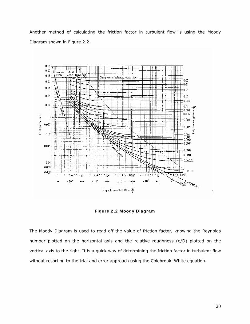
Another method of calculating the friction factor in turbulent flow is using the Moody

Diagram shown in Figure 2.2

Figure 2.2 Moody Diagram

The Moody Diagram is used to read off the value of friction factor, knowing the Reynolds

number plotted on the horizontal axis and the relative roughness (e/D) plotted on the

vertical axis to the right. It is a quick way of determining the friction factor in turbulent flow

without resorting to the trial and error approach using the Colebrook–White equation.

21

Similar to the non-dimensional friction factor f, another parameter F known as the

transmission factor is used in pipeline hydraulics. The dimensionless term, transmission

factor has an inverse relationship to the friction factor as indicated below:

F = 2/√ f (2.16)

Generally, the friction factor f has a value between 0.008 and 0.10. Therefore, using the

above equation we can deduce that the transmission factor F will have values approximately

in the range of 6 to 22. It can be stated that since the pressure drop due to friction is

proportional to the friction factor, it will decrease with increase in the value of the

transmission factor.

The Darcy equation discussed earlier is not convenient for pipeline calculations since it does

not employ common pipeline units, such as pressure in psi and flow in bbl/h. Therefore, the

following equation is generally used when dealing with pipelines transporting crude oils and

refined petroleum products. Pressure drop Pm, in psi per mile of pipe length, is calculated for

a given flow rate, pipe inside diameter, liquid specific gravity and the friction factor from:

Pm = 0.2421 (Q/F)2 Sg/D5 (2.17)

where Q is the flow rate in bbl/day and F is the dimensionless transmission factor. The liquid

specific gravity is Sg and the pipe inside diameter D is in inches.

In terms of the friction factor f, the equation for pressure drop becomes:

Pm = 0.0605 f Q2 (Sg/D5) (2.18)

When the flow rate is in bbl/h and gal/min, the equations for Pm are as follows:

Pm = 139.45 (Q/F)2 Sg/D5 for Q in bbl/h (2.19)

Pm = 284.59 (Q/F)2 Sg/D5 for Q in gal/min (2.20)

22

In SI units the pressure drop due to friction Pkm expressed in kPa/km is calculated from the

following equations:

Pkm = 6.2475 x 1010 f Q2 (Sg/D5) (2.21)

Pkm = 24.99 x1010 (Q/F)2 (Sg/D5) (2.22)

where the liquid flow rate Q is in m3/h and the pipe inside diameter D is in mm.

Remember in all the equations F and f are related by Equation 2.16. Since F and f are

inversely related, we can state that the higher the transmission factor, the higher will be the

throughput Q. In contrast, the higher the friction factor, the lower the value of Q. This flow

rate is directly proportional to f.

Example 6

Calculate the pressure drop per mile in an NPS 20 pipeline, 0.500 inch wall thickness flowing

diesel (Sg = 0.85 and viscosity = 5.0 cSt) at 8,000 bbl/h. Assume pipe absolute roughness

= 0.002 inch.

Solution

First calculate the Reynolds number:

R = 92.24 (8000 x 24)/(5.0 x 19.0) = 186,422

Since the flow is turbulent, we can use Colebrook-White equation or the Moody diagram to

determine the friction factor.

The relative roughness = (e/D) = 0.002/19 = 0.000105. For this value of (e/D) and R =

186,422 we get the friction factor f from the Moody diagram as follows:

f = 0.0166

Therefore, the transmission factor is:

F = 2/(0.0166)1/2 = 15.52

23

The pressure drop per mile is:

Pm = 139.45 (8000/15.52)2 x 0.85/(19.0)5

= 12.72 psi/mi

The Hazen-Williams equation is commonly used in hydraulic analysis of water pipelines.

It is used to calculate the pressure drop in a water pipeline given the pipe diameter and flow

rate, taking into account a the internal condition of the pipe using the dimensionless

parameter C. This parameter is called the Hazen-Williams C factor and is a function of the

internal roughness of the pipe. Unlike the friction factor, the C factor increases with the

smoothness of the pipe. In this regard it is more comparable to the transmission factor F

discussed earlier. Values of C range from 60 to 150 or more depending upon the pipe

material and roughness as indicated in Table 2.1

Pipe Material C-factor

Smooth Pipes (All metals) 130-140

Smooth Wood 120 Smooth Masonry 120 Vitrified Clay 110 Cast Iron (Old) 100 Iron (worn/pitted) 60-80 Polyvinyl Chloride (PVC) 150 Brick 100

Table 2.1 Hazen-Williams C factors

Although the Hazen-Williams equation is mostly used in water pipelines, today many

companies use it to calculate the pressure drop in pipelines transporting refined petroleum

products such as gasoline and diesel. For example, when used with water pipelines a C

value of 110 or 120 may be used and with gasoline and diesel typical values for C are 150

and 125, respectively. It must be noted that historically the value of C used is based on

24

experience with the particular liquid and pipeline and, therefore, varies from pipeline to

pipeline and with the company. However, the Colebrook-White equation is also used for

most liquids and a comparison can be made with Hazen-Williams equation as illustrated in

an example later. The classical form of the Hazen-Williams equation for pressure drop in

water pipelines is as follows:

h = 4.73 L (Q/C)1.852 / D4.87 (2.23)

where h is the head loss due to friction in ft of water. The pipe length L and diameter D are

both in ft and the flow rate Q is in ft3/s.

A more commonly used version of the Hazen-Williams equation is as follows:

Q = 6.7547 x 10-3 (C) (D)2.63 (h )0.54 (2.24)

where Q is in gal/min, D is in inches, and h is the head loss due to friction in ft of liquid per

1000 ft of pipe.

Another version of the Hazen-Williams equation in common pipeline units is as follows:

Q = 0.1482(C) (D)2.63(Pm /Sg)0.54 (2.25)

where Q is in bbl/day, D is in inches, and Pm is the pressure drop due to friction in psi/mi of

pipe. The specific gravity Sg is included so that it can be used for liquids other than water.

In SI Units, the Hazen-Williams formula is as follows:

Q = 9.0379x10-8 (C)(D)2.63(Pkm/Sg)0.54 (2.26)

where Q is in m3/h, D is in mm, and Pkm is the pressure drop due to friction in kPa/km.

Example 7

Calculate the pressure drop per mile in an NPS 20 pipeline, 0.500 inch wall thickness flowing

water at 7,500 gal/min. Use Hazen-Williams equation and C = 120.

25

Solution

Substituting the given values in Equation 2.24, the head loss h can be calculated as follows:

7500 = 6.7547 x 10-3 (120) (19.0)2.63 (h )0.54

Solving for h, we get:

h = 13.09 ft/1000 ft of pipe

Therefore, the pressure drop per mile, Pm is:

Pm = (13.09 x 1.0 / 2.31) x (5280/1000) = 29.92 psig/mi

For comparison, we will also calculate the pressure drop using the Colebrook-White equation

as follows:

First calculate the Reynolds number, considering the viscosity of water as 1.0 cSt.

R = 3160 x 7500 / (1.0 x 19.0) = 1,247,368

Since the flow is turbulent we can use the Colebrook-White equation or the Moody diagram

to determine the friction factor. We will also assume an absolute pipe roughness of 0.002 in.

The relative roughness = (e/D) = 0.002/19 = 0.000105. For this value of (e/D) and R =

1,247,368, we get the friction factor f from the Moody diagram as follows:

f = 0.0135

Therefore, the transmission factor is:

F = 2/(0.0135)1/2 = 17.21

The pressure drop per mile is:

Pm = 284.59 (7500/17.21)2 1.0/(19.0)5

= 21.83 psi/mi

So far we have discussed the two popular pressure drop formulas used in the pipeline

industry. The Colebrook–White equation is applicable for all liquids over a wide range of

Reynolds numbers. The Hazen-Williams equation originally developed for water pipelines is

26

now used with refined petroleum products as well. Several other pressure drop equations

are used in the crude oil and petroleum business and it would be useful to summarize them

here.

The Miller equation is used in crude oil pipelines and does not consider the Reynolds

number or pipe roughness. It requires an iterative solution to calculate the pressure drop Pm

from a given flow rate, liquid properties and pipe diameter. The most common form of the

Miller equation is as follows:

Q = 4.06 (M) (D5Pm/Sg)0.5 (2.27)

The parameter M is defined as follows:

M = Log10(D3SgPm/cp2 ) + 4.35 (2.28)

where the flow rate Q is in bbl/day and the liquid viscosity cP is in centipoise. All other

symbols have been defined before.

It can be seen that M depends on Pm and is also found in the equation connecting Q and Pm.

Therefore, from a given value of pressure drop Pm, M can be calculated and Q can be found

using equation 2.27. However, if Pm is unknown, to calculate Pm from a given value of flow

rate, pipe diameter and liquid properties, we must use a trial and error approach for solving

for Pm using the intermediate parameter M. The method is to assume a value of Pm and

calculate the corresponding value of M. Substituting this value of M in Equation 2.28 we can

solve for a new value of Pm. This forms the second approximation which can then be used to

calculate a new value of M and then a better value of Pm. The process is repeated until

successive values of Pm are within 0.001.

In SI Units, the Miller Equation is expressed as follows:

Q = 3.996 x 10-6 (M) (D5Pm/Sg)0.5 (2.29)

27

And the parameter M is defined as follows:

M = Log10(D3SgPm/cp2 ) - 0.4965 (2.30)

where all items have been defined previously.

The MIT equation developed jointly by Shell and MIT, sometimes known as Shell-MIT

equation is used in heavy crude oil pipelines that are heated to reduce the viscosity and

enhance pipe flow. It considers pipe roughness and uses a modified Reynolds number. The

Reynolds number is first calculated and then a modified Reynolds number obtained by

dividing it by 7742 as follows:

R = 92.24(Q)/(Dν) (2.31)

Rm = R/(7742) (2.32)

where the flow rate Q is in bbl/day and Viscosity ν is in cSt.

Depending upon the type of flow (laminar or turbulent) a friction factor is calculated using

the following equations:

f = 0.00207/Rm (for laminar flow) (2.33)

f = 0.0018 + 0.00662(1/Rm)0.355 (for turbulent flow) (2.34)

The friction factor f calculated above is not the same as the Darcy friction factor f calculated

using the Colebrook-White equation.

The pressure drop due to friction, Pm is then calculated from:

Pm = 0.241 (f SgQ2)/D5 (2.35)

All symbols have been defined previously.

In SI Units, the MIT Equation is stated as follows:

Pm = 6.2191 x 1010 (f SgQ2)/D5 (2.36)

where all symbols have been defined previously.

28

Example 8

Calculate the pressure drop per mile in an NPS 16 pipeline, 0.250 inch wall thickness flowing

crude oil (Sg = 0.895 and viscosity = 15.0 cSt) at 100,000 bbl/day. Assume pipe absolute

roughness = 0.002 inch. Compare the results using the Colebrook-White, Miller and MIT

equations.

Solution

Pipe inside diameter D = 16.0 – 2 x 0.250 = 15.50 in.

Next, calculate the Reynolds number:

R = 92.24 x 100000/(15.0 x 15.50) = 39,673

Since the flow is turbulent we use the Colebrook-White equation in the first case to

determine the friction factor.

The relative roughness = (e/D) = 0.002/15.5 = 0.000129

1/ √f = -2 Log10[(0.000129/3.7) + 2.51/(39673 √f )]

Solving for f by trial and error we get:

f = 0.0224

The pressure drop due to friction using the Colebrook-White equation is:

Pm = 0.0605 x 0.0224 x (100000)2 (0.895/(15.5)5)

=13.56 psi/mi

For the Miller equation we assume Pm = 14 psi/mi as the first approximation. Then

calculating the parameter M as follows:

M = Log10((15.5)3 0.895 x 14 /(15 x 0.895)2 ) + 4.35

where viscosity in cP = 15 x 0.895 = 13.425

Therefore, M = 6.7631

Next calculate the value of Pm from Equation 2.27:

100000 = 4.06 x 6.7631 x [(15.5)5Pm/0.895]0.5

29

Solving for Pm, we get:

Pm = 13.27 psi/mi, compared to the assumed value of 14.0.

Recalculating M from this latest value of Pm, we get:

M = Log10((15.5)3 0.895 x 13.27 /(15 x 0.895)2 ) + 4.35

Therefore, M = 6.74

Next calculate the value of Pm from Equation 2.27:

100,000 = 4.06 x 6.74 x [(15.5)5Pm/0.895]0.5

Solving for Pm, we get:

Pm = 13.36 psi/mi

Repeating the iteration once more, we get the final value of the pressure drop with the

Miller Equation as:

Pm = 13.35 psi/mi

Next we calculate the pressure drop using MIT equation.

The modified Reynolds number is:

Rm = R/7742 = 39673/7742 = 5.1244

Since R>4,000, the flow is turbulent and we calculate the MIT friction factor from Equation

2.34 as:

f = 0.0018 + 0.00662(1/5.1244)0.355 = 0.0055

The pressure drop due to friction is calculated from Equation 2.35:

Pm = 0.241 x 0.0055 x 0.895 x (100000)2/(15.5)5

= 13.32 psi/mi

Therefore, in summary the pressure drop per mile using the three equations are as follows:

Pm = 13.56 psi/mi using Colebrook-White equation

Pm = 13.35 psi/mi using Miller equation

Pm = 13.32 psi/mi using MIT equation

30

Finally it is seen that in this case all three pressure drop equations yield approximately the

same value for psi/mi with the Colebrook-White equation being the most conservative

(highest pressure drop for given flow rate).

Using the previously discussed equations such as Colebrook-White, Hazen-Williams, etc. we

can easily calculate the frictional pressure drop in a straight piece of pipe. Many

appurtenances such as valves and fittings installed in pipelines also contribute to pressure

loss. Compared to several thousand feet (or miles) of pipe, the Pressure Losses through

fittings and valves are small. Therefore, such pressure drops through valves, fitting and

other appurtenances are referred to as minor losses. Such losses may be calculated in a

couple of different ways.

Using the equivalent length concept, the valve or fitting is said to have the same frictional

pressure drop as that of a certain length of straight pipe. Once the equivalent length of the

device is known, the pressure drop in that straight length of pipe can be calculated. For

example, a gate valve is said to have an equivalent length to the diameter ratio of 8. This

means that a 16 inch gate valve has the same amount of pressure drop as a straight piece

of a 16 inch pipe with a length of 8 x 16 or 128 inches. Therefore, to calculate the pressure

drop in a 16 inch gate valve at 5,000 bbl/h flow rate we would simply calculate the psi/mi

value in a 16 inch pipe and use proportion as follows:

Let pressure drop in the 16 inch pipe = 12.5 psi/mi

Pressure drop in the 16 inch gate valve =12.5 x 128 /(5280 x 12) = 0.0253 psi/mi

It can be seen that the minor loss through a gate valve is indeed small in comparison with,

say, 1000 ft of 16 inch pipe (12.5 x 1000/5280 = 2.37 psi).

31

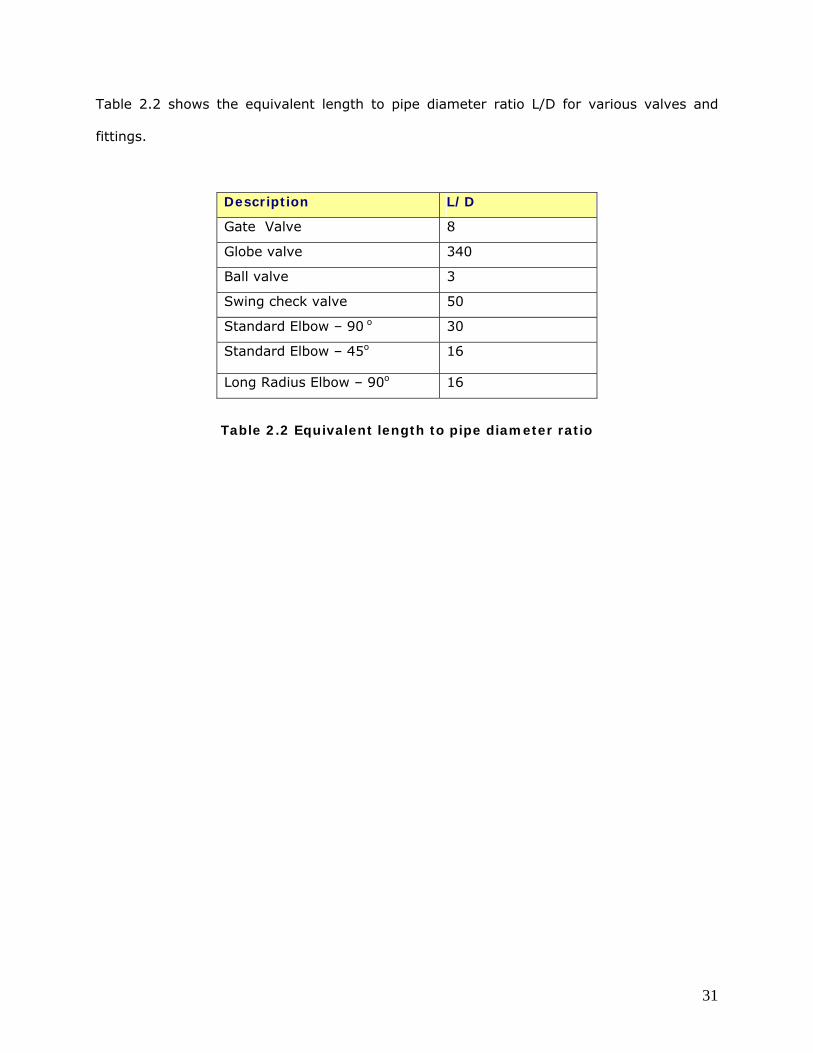
Table 2.2 shows the equivalent length to pipe diameter ratio L/D for various valves and

fittings.

Description L/D

Gate Valve 8

Globe valve 340

Ball valve 3

Swing check valve 50

Standard Elbow – 90 o 30

Standard Elbow – 45o 16

Long Radius Elbow – 90o 16

Table 2.2 Equivalent length to pipe diameter ratio

32

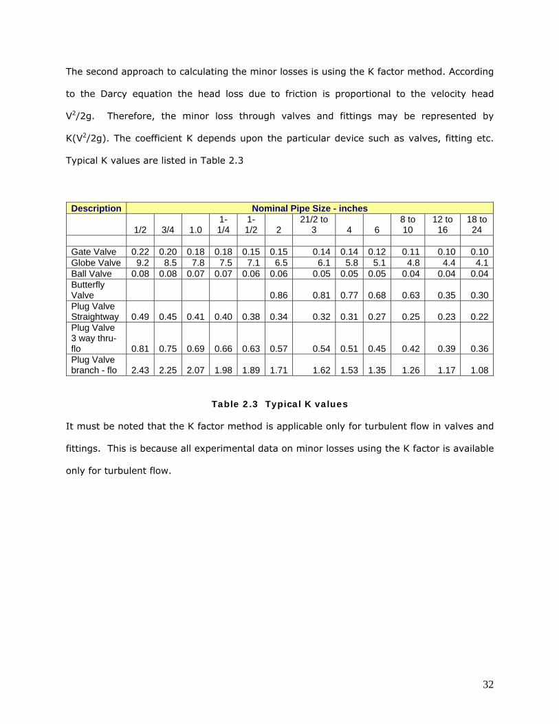
The second approach to calculating the minor losses is using the K factor method. According

to the Darcy equation the head loss due to friction is proportional to the velocity head

V2/2g. Therefore, the minor loss through valves and fittings may be represented by

K(V2/2g). The coefficient K depends upon the particular device such as valves, fitting etc.

Typical K values are listed in Table 2.3

Description Nominal Pipe Size - inches

1/2 3/4 1.0 1-1/4

1-1/2 2

21/2 to 3 4 6

8 to 10

12 to 16

18 to 24

Gate Valve 0.22 0.20 0.18 0.18 0.15 0.15 0.14 0.14 0.12 0.11 0.10 0.10Globe Valve 9.2 8.5 7.8 7.5 7.1 6.5 6.1 5.8 5.1 4.8 4.4 4.1Ball Valve 0.08 0.08 0.07 0.07 0.06 0.06 0.05 0.05 0.05 0.04 0.04 0.04Butterfly Valve 0.86 0.81 0.77 0.68 0.63 0.35 0.30Plug Valve Straightway 0.49 0.45 0.41 0.40 0.38 0.34 0.32 0.31 0.27 0.25 0.23 0.22Plug Valve 3 way thru-flo 0.81 0.75 0.69 0.66 0.63 0.57 0.54 0.51 0.45 0.42 0.39 0.36Plug Valve branch - flo 2.43 2.25 2.07 1.98 1.89 1.71 1.62 1.53 1.35 1.26 1.17 1.08

Table 2.3 Typical K values

It must be noted that the K factor method is applicable only for turbulent flow in valves and

fittings. This is because all experimental data on minor losses using the K factor is available

only for turbulent flow.

33

3. Pressure Required to Transport

In the previous section we discussed various equations to calculate the pressure drop due to

friction in a pipeline transporting a liquid. For example in Example 6, we calculated that in

an NPS 20 pipeline transporting diesel at a flow rate of 8,000 bbl/h the pressure drop due to

friction was 12.72 psi/mi. If the pipeline was 50 miles long, the total pressure drop due to

friction will be 12.72 x 50 = 636 psi.

A B

50 psi

686 psi

50 miles

Flow rate 8,000 bbl/h

Pressure variation

Figure 3.1 Total pressure required to pump liquid

Consider now that the pipeline originates at Point A and terminates at Point B, 50 miles

away. Suppose the delivered product at Point B is required to be at a minimum pressure of

50 psi to account for pressure drop in the delivery tank farm and the tank head. If the

ground elevation is essentially flat, the total pressure required at the origin of the pipeline,

A is 636 + 50 = 686 psi. The pressure of 686 psi at A will drop to 50 psi at B due to the

friction in the 50 mile length of pipe as shown in Figure 3.1. If the ground profile was not

flat, and the elevation of A is 100 ft and that at B is 500 ft, additional pressure is needed at

A to overcome the elevation difference of (500-100) ft. Using the head to pressure

34

conversion equation, the 400 ft elevation difference translates to 400 x 0.85/2.31 or 147.2

psi, considering the specific gravity of diesel as 0.85. This elevation component amounting

of 147.2 psi must then be added to the 686 psi resulting in a total pressure of 833.2 psi at A

in order to deliver the diesel at the terminus B at 50 psi pressure. This is illustrated in

Figure 3.2.

Hydraulic Pressure Gradient

Elevation Profile

A B

50 psi

833.2 psiC

D

100 ftElev

500 ft Elev400 ft = 147.2 psi

636 psi

50 psi

Figure 3.2 Components of total pressure

Thus we conclude that the total pressure required to transport a liquid from Point A to Point

B consists of three different components:

1. Friction Head

2. Elevation Head

3. Minimum Delivery Pressure

35

A graphical representation of the pressure variation along the pipeline from Point A to Point

B is depicted in Figure 3.3 and is known as the Hydraulic pressure gradient.

Terminus

Hydraulic Pressure Gradient

Elevation Profile

Peak

A B

PB

PA

D

E P

ress

ure

in f

t of

hea

d

Flow

C

Pmin

Figure 3.3 Hydraulic Pressure Gradient with peak

Since the liquid pressure in the pipeline is shown along with the pipe elevation profile, it is

customary to plot the pressures in ft of liquid head instead of pressure in psi. At any point

along the pipeline, the liquid pressure is represented by the vertical intercept between the

hydraulic gradient and the pipeline elevation at that point. This is shown at ED in Figure 3.3.

Of course, the pressure ED is in ft of liquid head and can be converted to psi, using the

specific gravity of the liquid.

In addition to the elevation difference between the origin A and the terminus B, there may

be drastic elevation changes along the pipeline, with peaks and valleys. In this case, we

must also ensure that the liquid pressure in the pipeline at any location does not fall below

36

zero (or some minimum value) at the highest elevation points. This is illustrated in Figure

3.3 where the peak in pipeline elevation at C shows the minimum pressure Pmin to be

maintained.

The minimum pressure depends upon the vapor pressure of the liquid at the flowing

temperature. For water, crude oils and refined petroleum products, since vapor pressures

are low and we are dealing with gauge pressures, a zero gauge pressure (14.7 psia) at the

high points can be tolerated. However, most companies prefer some non-zero gauge

pressure at the high points such as 10 to 20 psig. For highly volatile liquids with high vapor

pressures such as LPG, the minimum pressure along the pipeline must be maintained at

some number such as 200 to 250 psig to prevent vaporization and consequent two phase

flow. As the liquid flows through the pipeline, its pressure decreases due to friction and

increases or decreases depending upon the elevation change along the various points in the

pipeline profile. At some point such as C in Figure 3.3, the elevation is quite high and

therefore the pressure in the pipeline has dropped to a small value (Pmin) indicated by the

vertical intercept between the hydraulic gradient and the pipeline elevation at point C. If the

pressure at C drops below zero psig, vaporization of the liquid occurs and results in an

undesirable situation in liquid flow.

Due to the complexity of thermal hydraulics, we will restrict our analysis to steady state

isothermal flow only. This means that a constant flowing temperature of liquid is assumed

throughout the pipeline. Thermal flow occurs when the liquid temperature in the pipeline

varies from inlet to outlet. An example of thermal flow is the transportation of a heated

heavy crude oil. Due to high viscosity, the crude oil is heated before pumping to reduce its

viscosity and improve pipeline throughput. Therefore, at the beginning of the pipeline, the

liquid may be heated to 140°F and pumped through the pipeline. As the heated liquid flows

through the pipeline, heat is transferred from the liquid to the surrounding soil (buried

37

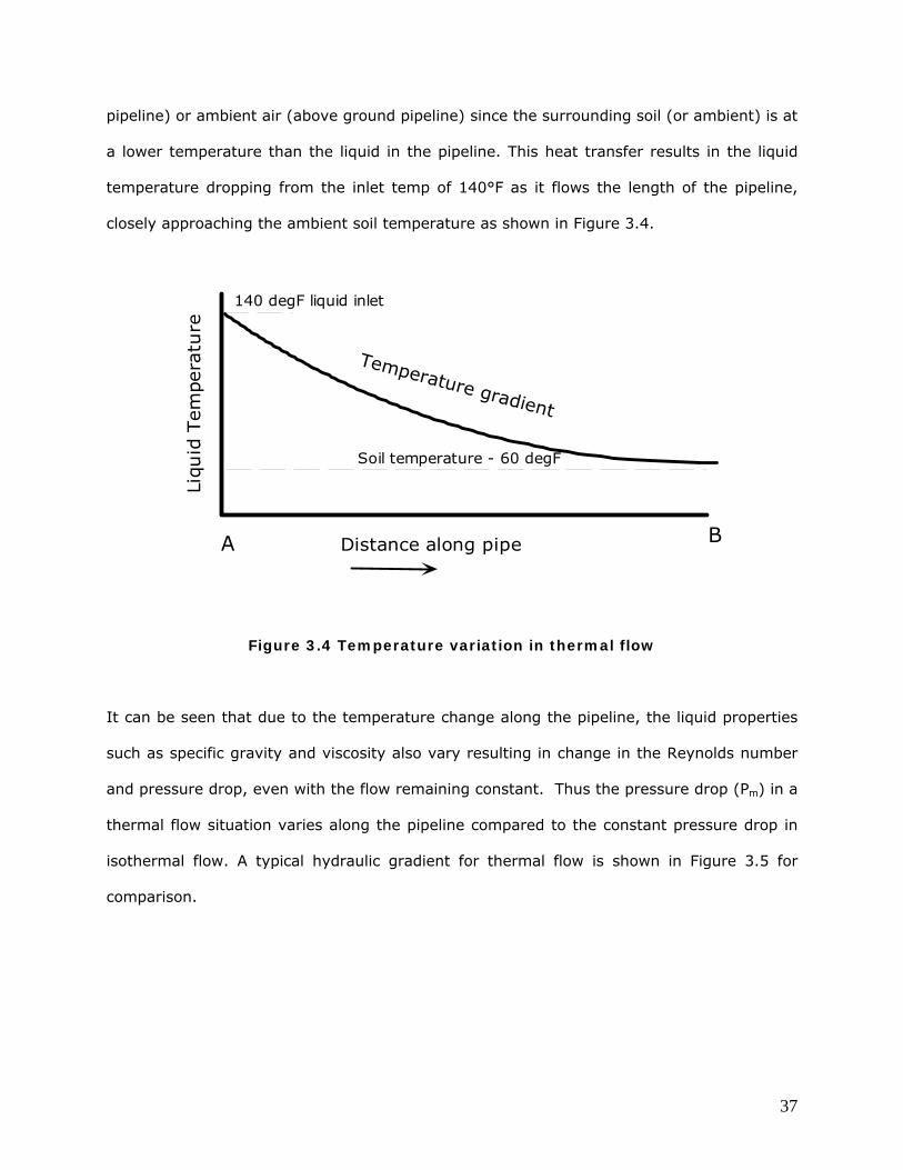
pipeline) or ambient air (above ground pipeline) since the surrounding soil (or ambient) is at

a lower temperature than the liquid in the pipeline. This heat transfer results in the liquid

temperature dropping from the inlet temp of 140°F as it flows the length of the pipeline,

closely approaching the ambient soil temperature as shown in Figure 3.4.

A B

Liqu

id T

empe

ratu

re

Distance along pipe

Soil temperature - 60 degF

140 degF liquid inlet

Temperature gradient

Figure 3.4 Temperature variation in thermal flow

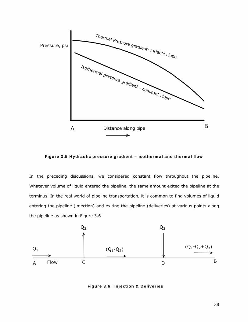
It can be seen that due to the temperature change along the pipeline, the liquid properties

such as specific gravity and viscosity also vary resulting in change in the Reynolds number

and pressure drop, even with the flow remaining constant. Thus the pressure drop (Pm) in a

thermal flow situation varies along the pipeline compared to the constant pressure drop in

isothermal flow. A typical hydraulic gradient for thermal flow is shown in Figure 3.5 for

comparison.

38

A BDistance along pipe

Isothermal pressure gradient - constant slope

Thermal Pressure gradient-variable slope

Pressure, psi

Figure 3.5 Hydraulic pressure gradient – isothermal and thermal flow

In the preceding discussions, we considered constant flow throughout the pipeline.

Whatever volume of liquid entered the pipeline, the same amount exited the pipeline at the

terminus. In the real world of pipeline transportation, it is common to find volumes of liquid

entering the pipeline (injection) and exiting the pipeline (deliveries) at various points along

the pipeline as shown in Figure 3.6

BA C D

Q1

Q2 Q3

(Q1-Q2)(Q1-Q2+Q3)

Flow

Figure 3.6 Injection & Deliveries

39

Liquid enters the pipeline at Point A at a flow rate Q1 and at some intermediate Point C a

certain volume Q2 is delivered out of the pipeline. The remaining volume (Q1-Q2) continues

on until at Point D a new volume of Q3 enters the pipeline. The resultant volume (Q1-Q2+Q3)

then continues to the terminus B where it is delivered out of the pipeline. The pressure

drops in each section of the pipeline such as AC, CD and DB must be calculated by

considering the individual flow rates and liquid properties in each section. Since flow Q2 is

delivered at C, the pipe sections AC and CD have the same liquid properties but different

flow rates for pressure drop calculations. The last section DB will have a different flow rate

and different liquid properties due to the combination of two different streams of liquid at

Point D. The total pressure required at A will be calculated by adding the pressure drop due

to friction for pipe sections AC, CD and DB and also adding the pressure required for pipe

elevation changes and including the minimum delivery pressure at the pipeline terminus.

Series and Parallel Pipes

Pipes are said to be in series when pipe of different diameters and lengths are connected

end to end and the liquid flows from the inlet of the first pipe to the outlet of the last pipe.

If there are no intermediate injections or deliveries, pipes in series will have flow as a

common parameter in all pipes. The total pressure required to pump a certain volume of

liquid through series pipes can be calculated by simply adding the pressure drop due to

friction in all pipe sections and including the elevation component and delivery pressure

component as before. This is illustrated in Figure 3.7

A B

QQ Q

Dia: D1Length: L1 Dia: D2

Length: L2Dia: D3Length: L3

Figure 3.7 Pipes in series

40

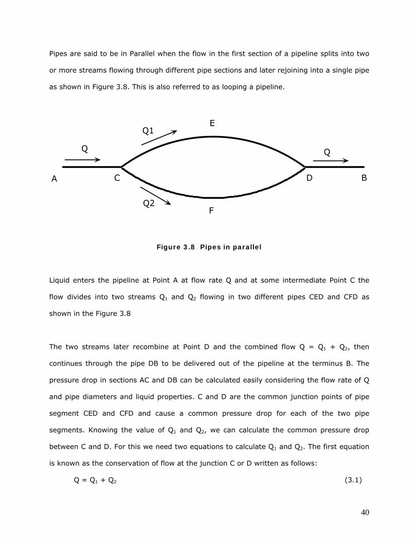
Pipes are said to be in Parallel when the flow in the first section of a pipeline splits into two

or more streams flowing through different pipe sections and later rejoining into a single pipe

as shown in Figure 3.8. This is also referred to as looping a pipeline.

F

A B

E

C D

Q

Q1

Q2

Q

Figure 3.8 Pipes in parallel

Liquid enters the pipeline at Point A at flow rate Q and at some intermediate Point C the

flow divides into two streams Q1 and Q2 flowing in two different pipes CED and CFD as

shown in the Figure 3.8

The two streams later recombine at Point D and the combined flow Q = Q1 + Q2, then

continues through the pipe DB to be delivered out of the pipeline at the terminus B. The

pressure drop in sections AC and DB can be calculated easily considering the flow rate of Q

and pipe diameters and liquid properties. C and D are the common junction points of pipe

segment CED and CFD and cause a common pressure drop for each of the two pipe

segments. Knowing the value of Q1 and Q2, we can calculate the common pressure drop

between C and D. For this we need two equations to calculate Q1 and Q2. The first equation

is known as the conservation of flow at the junction C or D written as follows:

Q = Q1 + Q2 (3.1)

41

The other equation connecting Q1 and Q2 comes from the common pressure drop between C

and D applied to each of the two pipes CED and CFD. Using the Darcy equation in the

modified form as indicated in Equation 2.17 we can write the following relationship for the

two pressure drops:

∆PCED = (Q1/F1)2 SgL1 /(D1) 5 (3.2)

where subscript 1 applies to the pipe section CED of length L1.

Similarly, for pipe section CFD of length L2 the pressure drop is:

∆PCFD = (Q2/F2)2 SgL2 /(D2) 5 (3.3)

Since both pressure drops are equal in parallel flow, and assuming the transmission factors

F1 and F2 are approximately equal, we can create the second equation between Q1 and Q2 as

follows:

(Q1)2 L1 /(D1) 5 = (Q2)2 L2 /(D2) 5 (3.4)

Using equations 3.1 and 3.4 we can solve for Q1 and Q2. The common pressure drop

between C and D can then be calculated using the equation for ∆PCED. We can then calculate

the total pressure drop by adding the individual pressure drops for pipe segment AC, DB

and ∆PCED. Of course, the elevation component must also be taken into account along with

the delivery pressure at B.

42

4. Pump Stations and Horsepower Required

In the previous sections we calculated the total pressure required to transport a certain

volume of liquid through a pipeline from point A to point B. If the pressure required is P at a

flow rate of Q, a pump will be needed at the origin A to provide this pressure. This pump will

be driven by an electric motor or engine that will provide the necessary horsepower (HP).

The pump HP required can be calculated from the pressure P and flow rate Q as follows:

HP = Q x P / Constant (4.1)

The constant will depend upon the units employed. In addition, since the pump is not 100%

efficient, we will need to take the efficiency into account to calculate the HP. Using common

pipeline units, if the pressure P is in psi and flow rate Q in bbl/day, the pump HP required is

given by:

HP = Q x P /(58776 x Effy) (4.2)

where the pump efficiency Effy is a decimal value less than 1.0. This HP is also called the

pump brake horsepower (BHP).

Strictly speaking, the pressure generated by the pump will be the difference between liquid

pressure on the suction side of the pump (Psuct) and the pump discharge pressure (Pdisch).

Therefore P in the HP equation must be replaced with (Pdisch – Psuct). This is called the

differential pressure generated by the pump.

Example 9

The suction and discharge pressures at a pump station are 50 psi and 875 psi, respectively,

when the liquid flow rate is 4,200 bbl/h. If the pump efficiency is 85%, calculate the

pumping HP required.

43

Solution

From Equation 4.2

BHP = (4200 x 24) x (875 – 50) /(58776 x 0.85)

When dealing with centrifugal pumps, the pressure developed by the pump is referred to as

pump head and expressed in ft of liquid head. The flow rate through the pump, also known

as pump capacity, is stated in gal/min. Most pump companies use water as the liquid to test

the pump, and the pump performance curves are therefore plotted in terms of water. The

HP equation discussed earlier can be modified in terms of pump head H in ft and flow rate Q

in gal/min for an efficiency of E (a decimal value) as follows:

Pump HP = Q x H x Sg /(3960 x E) (4.3)

where the liquid specific gravity is Sg.

Suppose the pump develops a head of 2,500 ft at a flow rate of 1,800 gal/min with an

efficiency of 82%, the pump HP required with water is calculated as:

HP = 1800 x 2500 x 1.0/(3960 x 0.82) = 1,386

If the pump is driven by an electric motor, the closest driver HP required in this case is

1,500 HP. It must be noted, that the motor efficiency would determine the actual electrical

power in Kilowatts (kW) required to run the 1,500 HP motor that is used to drive the pump

that requires 1,386 HP.

In a short pipeline such as the one discussed in an earlier example, the 50 mile pipeline

transporting diesel at 8,000 bbl/h required an originating pressure of 686 psi at A. Suppose

the pipeline was 120 miles long from Ashton to Beaumont and calculations show that at

8,000 bbl/h flow rate, the originating pressure at Ashton is 1,576 psi. If the pipe material

was strong enough to withstand the discharge pressure of 1,576 psi at Ashton, only one

44

pump station at Ashton will be needed to transport diesel at this flow rate from Ashton to

Beaumont. However, if the pipe material was such that the maximum allowable operating

pressure (MAOP) is limited to 1,440 psi, we would not be able to operate at 1,576 psi

discharge at Ashton. Therefore, by limiting the discharge pressure to the MAOP value, the

diesel throughput will fall below the 8,000 bbl/h value. If the throughput must be

maintained at 8,000 bbl/h while limiting pipeline pressures to MAOP, we can accomplish this

by installing a second pump station at some point between Ashton and Beaumont as shown

in Figure 4.1

AshtonPump Station

1516 psi

Pdisch

Beaumontterminus

Pdisch

50 psi

HamptonPump Station

120 mile8,000 bbl/h

Figure 4.1 Multiple pump stations

The intermediate pump station at Hampton is called the booster pump station and will be

located for hydraulic balance such that the same amount of energy is input into the liquid at

each pump station. In other words, the total HP required will be equally distributed between

the Ashton pump station and Hampton pump station. Since the flow rate is constant

throughout the pipeline (no intermediate injections or deliveries) hydraulic balance would

45

imply that each pump station discharges at approximately the same pressure as shown in

Figure 4.1.

Neglecting for the moment elevation difference along the pipeline and assuming the

minimum suction pressure at each pump station and the delivery pressure at Beaumont to

be equal to 50 psi, we can calculate the discharge pressure at each of the pump stations as

follows:

Pdisch + (Pdisch – 50) = 1576

or, Pdisch = 813 psi.

Therefore, each pump station will be operating at a discharge pressure of 813 psi.

Comparing this with the pipeline MAOP of 1,440 psi, we see that there is considerable room

to increase the discharge pressure and hence the flow rate. The maximum pipeline flow

rate will then occur when each pump station discharges at a pressure of 1,440 psi. It can be

seen that by increasing the discharge pressure to 1,440 psi causes the hydraulic gradient to

be steeper than that at 813 psi which corresponds to 8,000 bbl/h. If Hampton pump station

is located at a distance of 60 mi from Ashton, we can calculate the pressure drop due to

friction corresponding to the steeper gradient when discharging at 1,440 psi .

Since the hydraulic gradient is plotted in ft of head, the slope of the hydraulic gradient

represents the frictional head loss in ft/mi, which can also be expressed in psi/mi. From this

psi/mi, we can calculate the flow rate using Colebrook-White Equation as follows:

Pm = (1440 – 50) /60 = 23.17 psi/mi

This is the maximum slope of the hydraulic gradient when each pump station operates at

MAOP of 1,440 psig and elevation profile is neglected.

46

To calculate the flow rate from a given pressure drop we have to use a trial and error

approach. First calculate an approximate flow rate using the fact that Pm is proportional to

square of the flow rate Q from Equation 2.17. At 8,000 bbl/h the pressure drop is 12.72

psi/mi and at the unknown flow rate Q, Pm = 23.17:

23.17/12.72 = (Q/8000)2

Solving for Q we get:

Q = 10,797 bbl/h

Next using this flow rate we calculate the Reynolds number and friction factor using the

Colebrook-White Equation:

R = 92.24 (10797 x 24)/(5.0 x 19.0) = 251,600

Since the flow is turbulent we can use the Colebrook-White Equation or the Moody diagram

to determine the friction factor.

The relative roughness = (e/D) = 0.002/19 = 0.000105

For this value of (e/D) and R = 251,600 we get the friction factor f from the Moody diagram

as follows:

f = 0.0159

Therefore, the transmission factor is:

F = 2/(0.0159)1/2 = 15.86

The pressure drop per mile is therefore calculated from Equation 2.9:

Pm = 139.45 (10797/15.86)2 x 0.85/(19.0)5

= 22.19 psig/mi

Compare this with 23.17 psi/mi calculated from the pressure gradient. Therefore, the flow

rate has to be increased slightly higher to produce the required pressure drop.

Next approximate the flow rate, using proportions, since flow rate is proportional to the

square root of the pressure drop.

Q = 10797(23.17/22.19) 1/2 = 11,033 bbl/h

47

Recalculating the Reynolds number and friction factor we finally get the required flow rate

as 11,063 bbl/h. Thus, in the two pump station configuration the maximum flow rate

possible without exceeding MAOP is 11,063 bbl/h. The pump HP required depends upon the

liquid properties such as gravity and viscosity. It can be seen from Equation 4.3 that the

pump HP is directly proportional to liquid specific gravity. The effect of viscosity can be

explained by realizing that the pressure drop with a high viscosity liquid is generally higher

than when pumping a low viscosity liquid such as water. Therefore the pressure required to

pump a high viscosity liquid is greater than that required with a low viscosity liquid. It

follows then that the HP required to pump a heavy product will also be higher. When we

discuss centrifugal pump performance curves in the next section, the effect of viscosity will

be explained in more detail.

The hydraulic horsepower represents the pumping HP when the efficiency is considered to

be 100%. The Brake horsepower (BHP), on the other hand is the actual HP demanded by

the pump taking into account the pump efficiency.

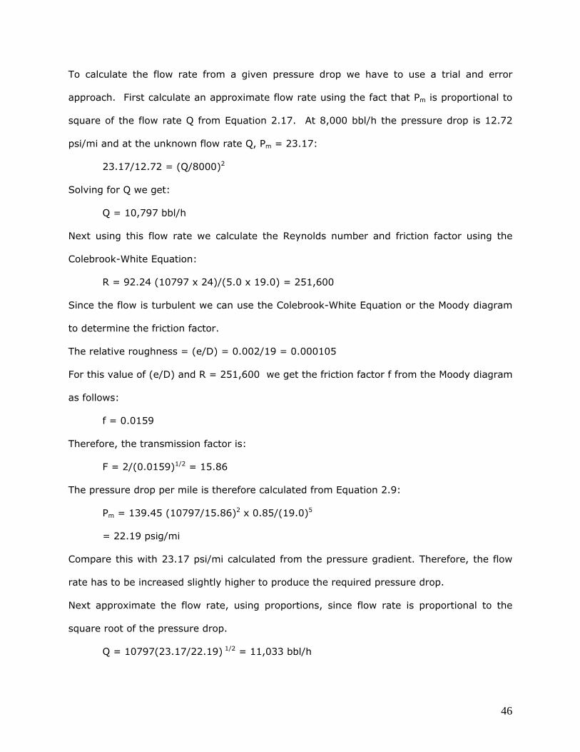
Pipeline System Head Curve

In the previous sections we calculated the total pressure required at the beginning of a

pipeline to transport a liquid at a certain flow rate to the pipeline terminus at a specified

delivery pressure. This pressure at the pipeline origin will increase as the flow rate is

increased, and hence we can develop a curve showing the pipeline pressure versus flow rate

for a particular pipeline and liquid pumped. This curve is referred to as the pipeline System

Head Curve or simply the System Curve for this specific product. Generally the pressure

is plotted in psi or ft of liquid head. The latter units for pressure is used when dealing with

centrifugal pumps. Figure 4.2 shows typical System Head Curves (in psi) for a pipeline

considering two products, gasoline and diesel. It can be seen that at any flow rate the

pressure required for diesel is higher than that for gasoline.

48

Pressure

Flow Rate

Gasoline

Diesel

Figure 4.2 Pipeline System Head Curves

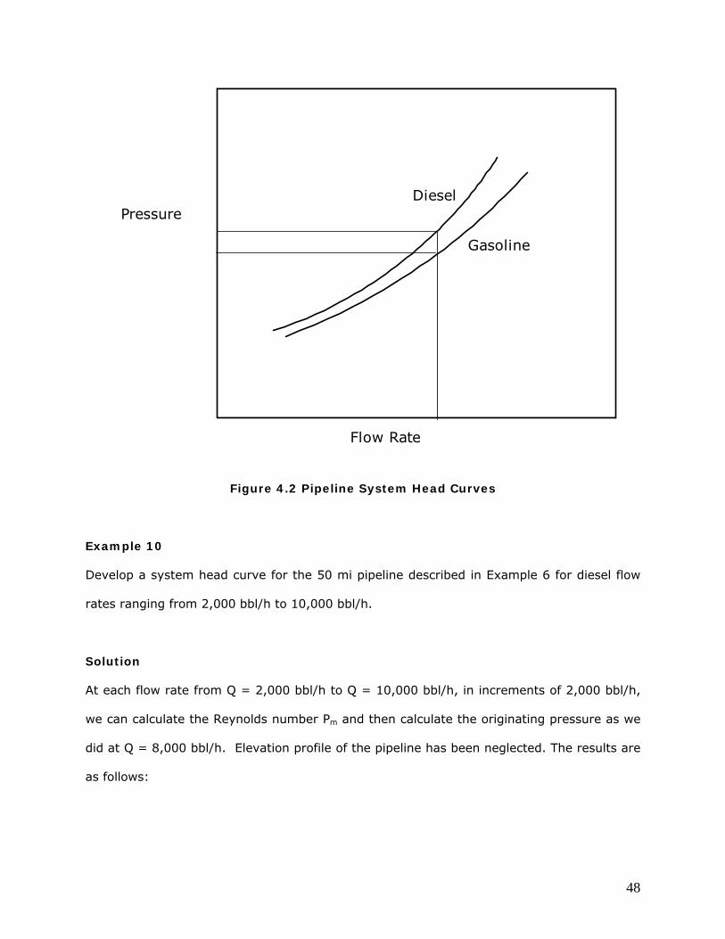
Example 10

Develop a system head curve for the 50 mi pipeline described in Example 6 for diesel flow

rates ranging from 2,000 bbl/h to 10,000 bbl/h.

Solution

At each flow rate from Q = 2,000 bbl/h to Q = 10,000 bbl/h, in increments of 2,000 bbl/h,

we can calculate the Reynolds number Pm and then calculate the originating pressure as we

did at Q = 8,000 bbl/h. Elevation profile of the pipeline has been neglected. The results are

as follows:

49

System Head Curve

0

200

400

600

800

1000

1200

2000 4000 6000 8000 10000

Flow rate, bbl/h

Pre

ssur

e, p

si

Q 2,000 4,000 6,000 8,000 10,000

Pt 102 230 426 686 1011

The system head curve is plotted below:

50

5. Pump Analysis

Pumps are used to produce the pressure required to transport a liquid through a pipeline.

Both centrifugal pumps and reciprocating pumps are used in pipeline applications.

Reciprocating pumps, also known as positive displacement or PD pumps produce high

pressures at a fixed flow rate depending upon the geometry of the pump. Centrifugal pumps

on the other hand are more flexible and provide a wider range of flow rates and pressures.

Centrifugal pumps are more commonly used in pipeline applications and will be discussed in

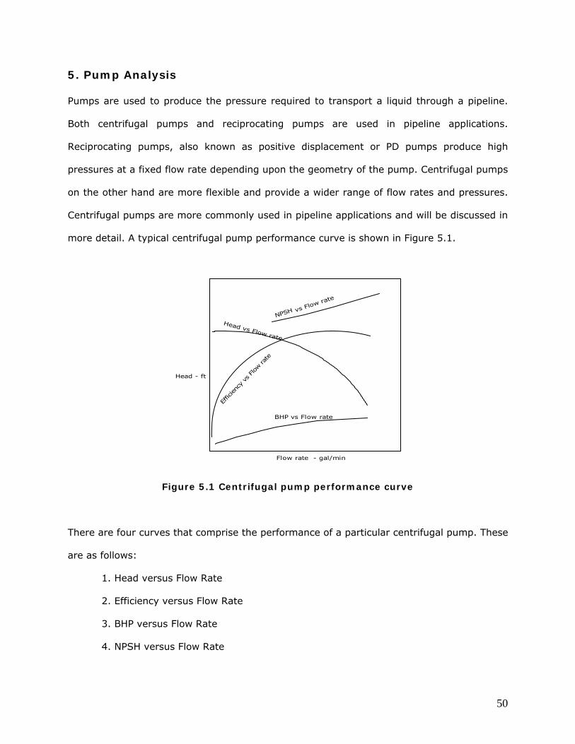
more detail. A typical centrifugal pump performance curve is shown in Figure 5.1.

Head - ft

Flow rate - gal/min

Head vs Flow rate

Effic

ienc

y vs

Flow

rate

BHP vs Flow rate

NPSH vs Flow rate

Figure 5.1 Centrifugal pump performance curve

There are four curves that comprise the performance of a particular centrifugal pump. These

are as follows:

1. Head versus Flow Rate

2. Efficiency versus Flow Rate

3. BHP versus Flow Rate

4. NPSH versus Flow Rate

51

Pump vendors use the term capacity when referring to the flow rate. It can be seen that in a

typical centrifugal pump, the head (or differential pressure) generated by the pump

decreases as the flow rate (also known as pump capacity) increases. This is known as a

drooping head versus flow characteristic. The efficiency, on the other hand, increases as the

flow rate increases and reaches a peak value (known as the best efficiency point or BEP)

and falls off rapidly with further increase in flow rate. The BHP also increases with increase

in flow rate. As mentioned before, centrifugal performance curves are generally plotted

considering water as the liquid pumped. Therefore, the BHP is calculated considering specific

gravity = 1.0.

The NPSH curve also increases with increase in flow rate. The term NPSH refers to Net

Positive Suction Head and is a measure of the minimum suction head required at the suction

of the pump impeller at any flow rate. NPSH is a very important parameter when dealing

with centrifugal pumps particularly when pumping volatile liquids. It will be discussed in

more detail later.

When pumping highly viscous liquids the centrifugal pump performance curves (for water)

must be adjusted or corrected for the liquid viscosity. This is done using the Hydraulic

Institute charts. A typical viscosity corrected performance curve chart is shown in Figure

5.2.

52

Figure 5.2 Viscosity corrected pump performance

It can be seen that the effect of viscosity is to reduce the head and efficiency at any flow

rate compared to that for water. On the other hand the BHP required increases with the

viscosity. When selecting a centrifugal pump for a particular application the objective would

be to pick a pump that provides the highest efficiency at the desired flow rate. Hence, the

pump curve would be selected such as the head and flow requirements are satisfied close to

and to the left of the BEP on the pump curve.

Typically, in a centrifugal pump, the pump impeller has a certain diameter but for the same

pump case, the impeller may be replaced with a smaller or larger impeller within certain

limits. For example, a centrifugal pump may have a rated impeller diameter of 10 inches

and produce a certain head versus flow characteristics similar to that depicted in Figure 5.3.

53

Figure 5.3 Pump performance at different impeller diameters

However, the same pump may be outfitted with an impeller as small as 8 inch diameter or

as large as 12 inch diameter Each of these impellers will proportionately reduce or increase

the performance characteristics. The performance of a centrifugal pump at different impeller

diameters generally follows the Affinity laws. This means that when going from a 10 inch

impeller diameter to a 12 inch diameter, the flow and head follow the Affinity Laws as

described below.

For an impeller size change from D1 to D2:

Q2/Q1 = D2/D1 for flow rates (5.1)

and H2/H1 = (D2/D1)2 for heads (5.2)

Head - ft

Flow rate - gal/min

Head

8"

10"

12"

54

Thus, the flow rate is directly proportional to the impeller diameter, and the head varies

directly as the square of the impeller diameter. The efficiency curves at the two different

impeller sizes will remain practically the same. Similar to impeller diameter variation, pump

speed changes also follow the Affinity laws as follows:

For an impeller speed change from N1 to N2 :

Q2/Q1 = N2/N1 for flow rates (5.3)

and H2/H1 = (N2/N1)2 for heads (5.4)

Thus the flow rate is directly proportional to the pump speed while the head is proportional

to the square of the pump speed.

The Affinity laws for impeller diameter variation are applicable for small changes in diameter

only. However, the Affinity laws can be applied for a wide variation in pump speeds. For

example, we may apply the Affinity laws for an impeller size variation from 8 inch to 12 inch

with a rated impeller of 10 inch. Extrapolation to 6 inch and 16 inch will not be accurate.

On the other hand if the pump is rated at a speed of 3500 rpm, we can apply the Affinity

laws for speed variations from 800 rpm to 6,000 rpm. However, the higher speeds may not

be possible from a design stand point due to high centrifugal forces that are developed at

the high speeds.

Example 11

Using Affinity laws determine the performance of a pump at an impeller size of 11 inch

given the following performance at 10 inch impeller diameter:

Q 500 1000 1500 2000

H 2000 1800 1400 900

Solution

Impeller diameter ratio = 11/10 = 1.10

55

The flow rate multiplier is 1.10 and the head multiplier is 1.10 x 1.10 = 1.21

Applying Affinity laws we get the following performance for 11 inch impeller:

Q 550 1100 1650 2200

H 2420 2178 1694 1089

Earlier we briefly discussed the NPSH required for a centrifugal pump. As the flow rate

through the pump increases, the NPSH requirement also increases. It is therefore important

to calculate the available NPSH based upon the actual piping configuration for a particular

pump installation. The calculated NPSH represents the available NPSH and hence must be

greater than or equal to the minimum NPSH required for the pump at a particular flow rate.

We will illustrate this using the example below.

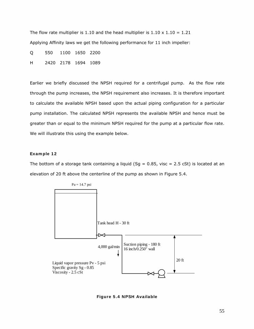
Example 12

The bottom of a storage tank containing a liquid (Sg = 0.85, visc = 2.5 cSt) is located at an

elevation of 20 ft above the centerline of the pump as shown in Figure 5.4.

Tank head H - 30 ft

Suction piping - 180 ft16 inch/0.250" wall4,000 gal/min

Liquid vapor pressure Pv - 5 psiSpecific gravity Sg - 0.85Viscosity - 2.5 cSt

20 ft

Pa = 14.7 psi

Figure 5.4 NPSH Available

56

The total length of a 16 inch pipe between the tank and the pump is 180 ft. The liquid level

in the tank is 30 ft and the vapor pressure of the liquid at a pumping temperature of 70°F is

5 psia. Considering an atmospheric pressure of 14.7 psia, calculate the NPSH available for

the pump at a flow rate of 4,000 gal/min.

Solution

Pump curve and system curve

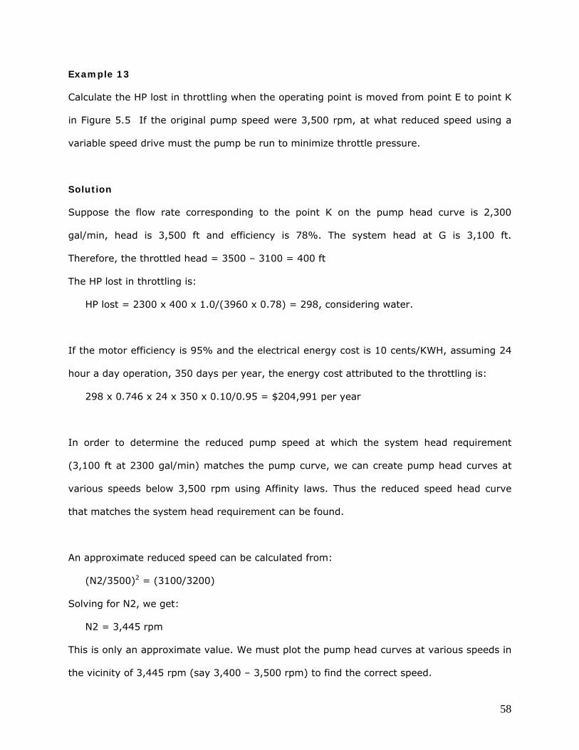
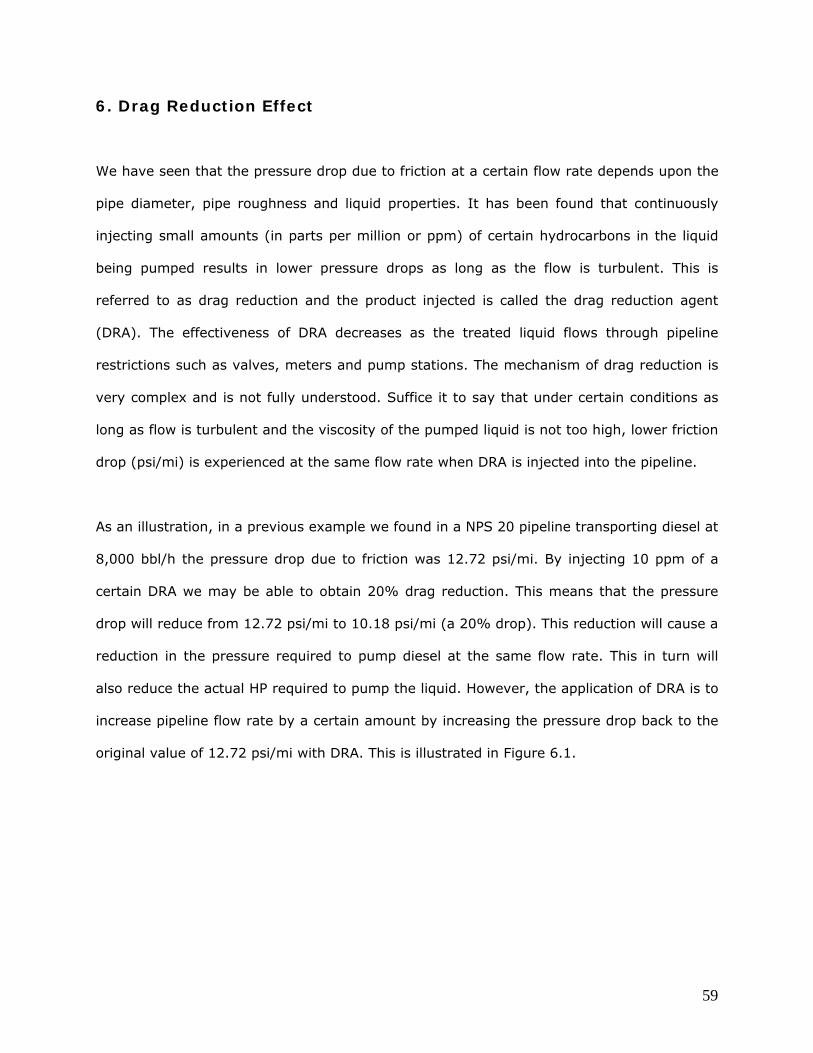
Consider a pipeline with a system head curve AB as shown in Figure 5.5

Head - ft

Flow Rate - gal/min

Pump Head

System

Head A

B

2500

E

F

40002000

3000

3200

4500

G

K

Figure 5.5 Pump curve and system curve – operating point

The pressure required at each flow rate is shown in ft of liquid head. At 2,000 gal/min the

head required is 3,000 ft whereas 4,000 gal/min requires 4,500 ft. A centrifugal pump head

curve CD shown superimposed on the system curve intersects the system curve at point E

as shown. At E, both the pump head and system head match and are equal to 3,200 ft. If

the corresponding flow rate is 2,500 gal/min we can say that the system requirements and

57

the pump capability at 2,500 gal/min are exactly equal. Hence point E represents the

operating point when this particular pump is used to pump the liquid through this pipeline.

If a lighter product is pumped instead, its system head curve will be lower than the first

liquid and hence will intersect the pump head curve at point F which represents a higher

flow rate and lower head. Plotting the pump efficiency curve along with the head curve we

can also determine the pump efficiency at the operating point and hence the HP required to

pump the product.

Suppose the operating point E represents a pressure that exceeds the allowable pipeline

pressure. In order to reduce the pressure to that represented by point G we have to reduce

the flow rate through the pump to some value Q1. This is accomplished by using a control

valve on the discharge of the pump. The reduced flow rate causes a difference in pump

head curve and system head curve equal to the length GK. This head represents the throttle

pressure at the flow rate Q1. The pump case pressure is the pressure developed by the

pump at flow rate Q1 and represented by point K on the pump head curve. Since the

throttle pressure is the amount of pump head wasted (GK), a certain amount of pump HP is

wasted as well. This HP lost due to throttling can be calculated easily knowing the flow rate

Q1, the throttle pressure and the pump efficiency at Q1. HP lost due to throttling at flow

rate Q1 is as follows:

HP= Q1 x HGK x Sg/(3960 x Effy) (5.5)

If the pump was driven by a variable speed motor we could lower the pump speed and

match the system head required at flow rate Q1. This is shown as a dotted head curve in

Figure 5.5. Obviously, with a variable speed pump, throttling is eliminated and therefore no

HP is lost. The system head curve requirement at point G at a flow rate of Q1 is exactly

matched by the dotted pump head curve at the reduced speed.

58

Example 13

Calculate the HP lost in throttling when the operating point is moved from point E to point K

in Figure 5.5 If the original pump speed were 3,500 rpm, at what reduced speed using a

variable speed drive must the pump be run to minimize throttle pressure.

Solution

Suppose the flow rate corresponding to the point K on the pump head curve is 2,300

gal/min, head is 3,500 ft and efficiency is 78%. The system head at G is 3,100 ft.

Therefore, the throttled head = 3500 – 3100 = 400 ft

The HP lost in throttling is:

HP lost = 2300 x 400 x 1.0/(3960 x 0.78) = 298, considering water.

If the motor efficiency is 95% and the electrical energy cost is 10 cents/KWH, assuming 24

hour a day operation, 350 days per year, the energy cost attributed to the throttling is:

298 x 0.746 x 24 x 350 x 0.10/0.95 = $204,991 per year

In order to determine the reduced pump speed at which the system head requirement

(3,100 ft at 2300 gal/min) matches the pump curve, we can create pump head curves at

various speeds below 3,500 rpm using Affinity laws. Thus the reduced speed head curve

that matches the system head requirement can be found.

An approximate reduced speed can be calculated from:

(N2/3500)2 = (3100/3200)

Solving for N2, we get:

N2 = 3,445 rpm

This is only an approximate value. We must plot the pump head curves at various speeds in

the vicinity of 3,445 rpm (say 3,400 – 3,500 rpm) to find the correct speed.

59

6. Drag Reduction Effect

We have seen that the pressure drop due to friction at a certain flow rate depends upon the

pipe diameter, pipe roughness and liquid properties. It has been found that continuously

injecting small amounts (in parts per million or ppm) of certain hydrocarbons in the liquid

being pumped results in lower pressure drops as long as the flow is turbulent. This is

referred to as drag reduction and the product injected is called the drag reduction agent

(DRA). The effectiveness of DRA decreases as the treated liquid flows through pipeline

restrictions such as valves, meters and pump stations. The mechanism of drag reduction is

very complex and is not fully understood. Suffice it to say that under certain conditions as

long as flow is turbulent and the viscosity of the pumped liquid is not too high, lower friction

drop (psi/mi) is experienced at the same flow rate when DRA is injected into the pipeline.

As an illustration, in a previous example we found in a NPS 20 pipeline transporting diesel at

8,000 bbl/h the pressure drop due to friction was 12.72 psi/mi. By injecting 10 ppm of a

certain DRA we may be able to obtain 20% drag reduction. This means that the pressure

drop will reduce from 12.72 psi/mi to 10.18 psi/mi (a 20% drop). This reduction will cause a

reduction in the pressure required to pump diesel at the same flow rate. This in turn will

also reduce the actual HP required to pump the liquid. However, the application of DRA is to

increase pipeline flow rate by a certain amount by increasing the pressure drop back to the

original value of 12.72 psi/mi with DRA. This is illustrated in Figure 6.1.

60

Head

Flow Rate

System

curve

- no DRA

A

B

System curve - with DRA

E

G

Pump Head Curve

Figure 6.1 Drag Reduction effect on system head curve

Without DRA, the operating point for the pipeline system curve and the pump curve is

shown as the point E. With DRA injection, the system curve slides to the right and below as

shown in the dashed system curve. The operating point thus shifts to the point G. At G, the

flow rate is higher than at E. However, at the increased flow, the pump HP required will also

increase. The drive HP must also be adequate to operate at this increased flow rate.

The quantity of DRA injected is in ppm. For example, if the pipeline flow rate is 8,000 bbl/h

and we are using 10 ppm of DRA, the actual DRA injection rate can be calculated as follows:

DRA ppm = 10 = (10/106) x 8000 = 0.08 bbl/h = 0.08 x 42 x 24 gal/day

or DRA injection rate = 80.64 gal/day

61

Therefore, for 10 ppm, we need to continuously inject DRA at the rate of 80.64 gal/day to

achieve the desired drag reduction.

One application of drag reduction is in a pipeline with multiple pump stations, which has a

bottleneck segment. Suppose there are three pump stations with two stations discharging

below MAOP while the third pump station discharges at MAOP as shown in Figure 6.2.

MAOP

D

PdPd

A

MAOP MAOP

B C

Figure 6.2 Pipeline bottleneck and DRA application

Due to this MAOP limit in the segment AB, the pipeline throughput is limited to some value

Q. If we increase the flow rate above Q, the discharge pressure at the critical pump station

(A) will exceed MAOP. Since this is not allowable, DRA can be injected into the bottleneck

pump station segment immediately downstream of A to reduce friction and hence the

discharge pressure as the flow rate is increased. Since the effectiveness of the DRA

diminishes from pump station to pump station, the other two pump stations (B and C) will

operate at higher discharge pressures than before at the increased flow rate. This may be

permissible to some extent since originally, these two pump stations were operating below

MAOP and there is still room left for the discharge pressure to reach the MAOP limit as

indicated by the dashed lines in the hydraulic gradient in Figure 6.2.

62

Once these two pump stations reach the MAOP limit, at some flow rate higher than Q, these

two segments BC and CD become the bottleneck segments. Any further increase in pipeline

throughput is possible only by using DRA in these two segments as well. Note that with

DRA injection in segment AB at the higher flow rate, the hydraulic gradient for AB will be

different from that of segment BC and CD, since the DRA effectiveness is only in segment

AB. As the DRA treated liquid flows through pump stations B and C, the DRA effectiveness is

lost due to the degradation of DRA.

The amount of DRA required in ppm to achieve a certain flow increase depends upon many

factors. For a particular pipeline, depending upon the liquid viscosity, gravity and the

Reynolds number, DRA effectiveness varies with flow rate. DRA vendors such as Baker

Petrolite and Conoco-Phillips have their own algorithms to calculate the percentage drag

reduction possible for a given DRA injection rate. In general, the percentage drag reduction

will increase with ppm of DRA up to some point known as maximum drag reduction (MDR).

For further details on this matter, contact one of the DRA vendors.

63

7. Batching different products So far in our hydraulic analysis we considered a single product flowing through a pipeline at

any time. In this section under flow injection and deliveries we also looked at two streams

of liquid commingled and transported through the pipeline as a single product. When

commingling of products is not acceptable, but multiple products have to be transported

simultaneously in a pipeline, we have what is known as batching. Consider a pipeline 100 mi

long, that has a line fill (total volume) capacity of 150,000 bbl. In a typical batching

situation, 80,000 bbl batch of gasoline will be followed by a 30,000 bbl batch of diesel and

40,000 bbl batch of jet fuel as shown in Figure 7.1

80 Mbbl

GasolineDieselJet fuel

30 Mbbl40 Mbbl

Figure 7.1 Batched pipeline

At the boundary of any two products there will be some commingling which will have to be

separated as the products reach the pipeline terminus. Generally, the commingled liquid is

switched to a slop tank while the pure products of gasoline, diesel and jet fuel will be

diverted to their respective tanks at the pipeline destination. It can be seen from Figure 7.1

that at any instant in the batched movement of products, the flow rate versus pressure drop

will depend upon the frictional pressure drops for each liquid that occupies a certain section

of the pipeline. If gasoline occupied the entire pipeline, the pressure drop in the 100 mi

pipeline segment will be calculated considering the specific gravity and viscosity of gasoline.

Being the lightest product of the three, the pressure drop at any flow rate will be the lowest

for gasoline. In comparison, if diesel filled the pipeline completely, the pressure drop will be

the highest at the same flow rate. Finally, with jet fuel filling the entire pipeline, the

64

pressure drop at the same flow rate will be a value between those for gasoline and diesel. If

we were to calculate separately the maximum flow rate possible for each product within the

MAOP limit of the pipeline, we may come up with the following flow rates:

Qmax = 8,700 bbl/h for gasoline

Qmax = 6,500 bbl/h for jet fuel

Qmax = 5,200 bbl/h for diesel

In the batched configuration the maximum flow rate possible will depend upon the amounts

of each products filling the pipeline. As a rough approximation we could use a weighted

average depending upon the batch volumes. If each product occupies a third of the pipeline

at any instant, the maximum flow rate in the batched configuration is approximately:

Qmax = (8700 + 6500 + 5200)/3 = 6,800 bbl/h

Of course, this is a simplistic approach to determining batched hydraulics of pipelines, and a

more accurate method is required to determine the flow rate possible in a batched pipeline.

Before we pursue this more accurate approach it will be instructive to determine the

approximate flow rate with the batched volumes defined earlier, shown in Figure 7.1.

The weighted average flow rate in this case can be calculated as follows:

Fraction of line fill for gasoline = 80000/150000 = 0.5333

Fraction of line fill for jet fuel = 40000/150000 = 0.2667

Fraction of line fill for diesel = 1 – (0.5333 + 0.2667) = 0.20

Therefore:

Qmax = (8700 x 0.5333) + (6500 x 0.2667) + (5200 x 0.20) = 7,413 bbl/h

65

8. Pipe Analysis

In the previous sections, we calculated the pressure needed to pump a certain flow rate of

liquid through a pipeline. We also briefly discussed that if the pressure required exceeds the

maximum allowable operating pressure (MAOP) of the pipeline, we will need to install

additional booster pump stations to provide the total pressure to pump the liquid, without

exceeding MAOP. The MAOP of a pipeline is the maximum safe internal pressure that the

pipeline can withstand without failure. This will depend upon the pipe material, diameter

and wall thickness. As the internal pressure is increased, the pipe material gets stressed

more and more and, ultimately, will undergo permanent deformation and will rupture.

Therefore it is very important to determine the safe internal pressure that the pipe can

withstand, without rupture, so that we may operate the pipeline safely.

The Barlow’s equation in a modified form is used to calculate this allowable internal pressure

as follows:

In USCS units, the internal design pressure in a pipe is calculated as follows:

P = (2 T x S x E x F)/D (8.1)

where P is the internal design pressure in psig. The pipe outside diameter D and wall

thickness T are in inches. S is the Specified Minimum Yield Strength (SMYS) of pipe material

in psig and E is the Seam Joint Factor, 1.0, for seamless and Submerged Arc Welded (SAW)

pipes. F is the Design Factor, usually 0.72, for liquid pipelines except that a design factor of

0.60 is used for pipes, including risers, on a platform located off shore or on a platform in

inland navigable waters. Similarly, a design factor of 0.54 is used for pipes that have been

subjected to cold expansion to meet the SMYS and subsequently heated, other than by

welding or stress relieving as a part of the welding, to a temperature higher than 900°F

(482°C) for any period of time or over 600°F (316°C) for more than one hour.

66

The above version of Barlow’s equation is described in Part 195 of US DOT code of Federal

Regulations, Title 49 and ASME/ANSI standard B31.4 for liquid pipelines.

In SI units, the internal design pressure equation can be written as:

P = (2 T x S x E x F)/D (8.2)

where P is the pipe internal design pressure in kPa. The pipe outside diameter D and wall

thickness T are in mm. S is the Specified Minimum Yield Strength (SMYS) of the pipe

material in kPa, and E and F are the same as before.

Once we know the safe internal working pressure for the pipe, a hydrostatic test pressure is

established. Generally, for liquid pipelines this test pressure is 125% of the allowable

working pressure. The hydrostatic test pressure is the pressure at which the pipeline is

tested for a specified period of time, usually 4 to 8 hours, depending upon the design code.

For above ground piping 4 hours is used, while buried pipelines are tested for 8 hours. In

the USA, the Department of Transportation (DOT) Code Part 195 applies for liquid pipelines.

Therefore, if the MAOP is 1,000 psig, the hydrotest pressure will be 1.25x1000 = 1250 psig.

The SMYS of the pipe material depends on the type of steel used in constructing the pipe.

The API 5L standard for pipe covers many grades: X-42, X-52, X-60, X-65, X-70 and X-80.

The number after the X represents the SMYS in thousands of psi. Thus X-60 pipe has an

SMYS of 60,000 psi.

For example, the MAOP for a 16 inch pipeline, 0.250 inch wall, constructed of X-52 pipe

material is:

P = (2 x 0.250 x 52000 x 1.0 x 0.72 ) / 16 = 1,170 psig

The hydrotest pressure is therefore:

1.25 x 1170 = 1,463 psig

67

References

1. Liquid Pipeline Hydraulics, E. Shashi Menon, Marcel Dekker, Inc. 2005 2. Piping Calculations Manual, E. Shashi Menon, McGraw – Hill, 2005 3. Elementary Fluid Mechanics, Vennard & Street. Sixth Edition. John Wiley and Sons,

1982. 4. Handbook of Hydraulics, Brater & King. McGraw-Hill, 1982 5. Pipeline Design for Hydrocarbons, Gases and Liquids. American Society of Civil

Engineers, 1975. 6. Cameron Hydraulic Data. Ingersoll-Rand, 1981 7. Flow of Fluids through Valves, Fittings and Pipes. Crane Company, 1976 8. V.S. Lobanoff and R.R. Ross. Centrifugal Pumps Design & Application. Gulf Publishing,

1985 9. Hydraulic Institute Engineering Data Book - Hydraulic Institute, 1979