132
1 Course Spectroscopy last updated: July 6 th , 2011 Marko Bertmer Faculty of Physics and Geosciences Leipzig University Linn´ estr. 5 04103 Leipzig, Germany

1
Course Spectroscopy
last updated: July 6th, 2011
Marko Bertmer
Faculty of Physics and Geosciences
Leipzig University
Linnestr. 5
04103 Leipzig, Germany

2

Contents
1 Introduction 9
1.1 Definition . . . . . . . . . . . . . . . . . . . . . . . . . . . . . . . . . 9
1.2 Historical development . . . . . . . . . . . . . . . . . . . . . . . . . . 10
1.3 Atomic spectra of hydrogen . . . . . . . . . . . . . . . . . . . . . . . 11
1.4 Electromagnetic spectrum . . . . . . . . . . . . . . . . . . . . . . . . 13
1.5 The Experimental Scientist . . . . . . . . . . . . . . . . . . . . . . . . 14
1.6 Literature . . . . . . . . . . . . . . . . . . . . . . . . . . . . . . . . . 15
1.7 Questions for Recapitulation . . . . . . . . . . . . . . . . . . . . . . . 16
1.8 References . . . . . . . . . . . . . . . . . . . . . . . . . . . . . . . . . 16
2 Absorption and Emission of Radiation 17
2.1 Electromagnetic Radiation . . . . . . . . . . . . . . . . . . . . . . . . 17
2.2 Absorption and Emission . . . . . . . . . . . . . . . . . . . . . . . . . 19
2.3 Black Body Radiation . . . . . . . . . . . . . . . . . . . . . . . . . . 20
2.4 Lifetime and Linewidth . . . . . . . . . . . . . . . . . . . . . . . . . . 25
2.5 Interaction of Matter with Electromagnetic Radiation . . . . . . . . . 30
2.6 Transition Probabilities . . . . . . . . . . . . . . . . . . . . . . . . . . 34
2.7 Fourier Transform . . . . . . . . . . . . . . . . . . . . . . . . . . . . . 35
2.8 Questions for Recapitulation . . . . . . . . . . . . . . . . . . . . . . . 38
2.9 References . . . . . . . . . . . . . . . . . . . . . . . . . . . . . . . . . 39
3 Structure and Symmetry 41
3.1 Quantum Mechanics of the Hydrogen Atom . . . . . . . . . . . . . . 41
3.2 Molecular Orbitals . . . . . . . . . . . . . . . . . . . . . . . . . . . . 47
3.3 Multi-Electron Systems, Term Symbol . . . . . . . . . . . . . . . . . 51
3

4 CONTENTS
3.4 Group Theory . . . . . . . . . . . . . . . . . . . . . . . . . . . . . . . 57
3.5 Questions for Recapitulation . . . . . . . . . . . . . . . . . . . . . . . 64
3.6 References . . . . . . . . . . . . . . . . . . . . . . . . . . . . . . . . . 65
4 Nuclear Magnetic Resonance (NMR) 67
4.1 Introduction . . . . . . . . . . . . . . . . . . . . . . . . . . . . . . . . 67
4.2 Basics of NMR . . . . . . . . . . . . . . . . . . . . . . . . . . . . . . 67
4.3 Experimental Setup . . . . . . . . . . . . . . . . . . . . . . . . . . . . 71
4.4 Relaxation . . . . . . . . . . . . . . . . . . . . . . . . . . . . . . . . . 71
4.4.1 Spin-Lattice Relaxation . . . . . . . . . . . . . . . . . . . . . 72
4.4.2 Spin-Spin Relaxation . . . . . . . . . . . . . . . . . . . . . . . 73
4.4.3 Bloch Equations . . . . . . . . . . . . . . . . . . . . . . . . . 75
4.4.4 Further Relaxation Times . . . . . . . . . . . . . . . . . . . . 76
4.5 Interactions . . . . . . . . . . . . . . . . . . . . . . . . . . . . . . . . 76
4.5.1 Chemical Shift . . . . . . . . . . . . . . . . . . . . . . . . . . 76
4.5.2 Indirect Dipolar Coupling . . . . . . . . . . . . . . . . . . . . 78
4.5.3 Direct Dipolar Coupling . . . . . . . . . . . . . . . . . . . . . 80
4.5.4 Quadrupolar Coupling . . . . . . . . . . . . . . . . . . . . . . 81
4.6 Experimental Flexibility . . . . . . . . . . . . . . . . . . . . . . . . . 82
4.6.1 MAS . . . . . . . . . . . . . . . . . . . . . . . . . . . . . . . . 83
4.6.2 Decoupling . . . . . . . . . . . . . . . . . . . . . . . . . . . . 84
4.6.3 Double Resonance . . . . . . . . . . . . . . . . . . . . . . . . 85
4.6.4 2D NMR . . . . . . . . . . . . . . . . . . . . . . . . . . . . . . 85
4.6.5 Magnetic Resonance Imaging . . . . . . . . . . . . . . . . . . 86
4.7 References . . . . . . . . . . . . . . . . . . . . . . . . . . . . . . . . . 87
5 Electron Spin Resonance (ESR) 89
5.1 Introduction . . . . . . . . . . . . . . . . . . . . . . . . . . . . . . . . 89
5.2 Experimental Setup . . . . . . . . . . . . . . . . . . . . . . . . . . . . 90
5.3 g-Factor . . . . . . . . . . . . . . . . . . . . . . . . . . . . . . . . . . 92
5.4 Zero Field Splitting . . . . . . . . . . . . . . . . . . . . . . . . . . . . 94
5.5 Hyperfine splitting . . . . . . . . . . . . . . . . . . . . . . . . . . . . 95
5.6 Hamilton operators . . . . . . . . . . . . . . . . . . . . . . . . . . . . 97
5.7 ENDOR . . . . . . . . . . . . . . . . . . . . . . . . . . . . . . . . . . 98

CONTENTS 5
5.8 References . . . . . . . . . . . . . . . . . . . . . . . . . . . . . . . . . 99
6 Rotational and vibrational spectroscopy 101
6.1 Rotational Spectroscopy . . . . . . . . . . . . . . . . . . . . . . . . . 101
6.1.1 Experimental Setup . . . . . . . . . . . . . . . . . . . . . . . . 101
6.1.2 Quantum Mechanical Description . . . . . . . . . . . . . . . . 102
6.1.3 Rigid and Non-Rigid Rotor . . . . . . . . . . . . . . . . . . . 104
6.1.4 Stark Effect . . . . . . . . . . . . . . . . . . . . . . . . . . . . 107
6.1.5 Line Intensities . . . . . . . . . . . . . . . . . . . . . . . . . . 108
6.2 Vibrational Spectroscopy . . . . . . . . . . . . . . . . . . . . . . . . . 109
6.2.1 Harmonic Oscillator . . . . . . . . . . . . . . . . . . . . . . . 109
6.2.2 Transition moment for IR and Raman Spectroscopy . . . . . . 111
6.2.3 Anhoarmonic Oscillator . . . . . . . . . . . . . . . . . . . . . 112
6.2.4 Rotation-Vibration Spectra . . . . . . . . . . . . . . . . . . . 112
6.2.5 Experimental Setup . . . . . . . . . . . . . . . . . . . . . . . . 114
6.2.6 Polyatomic Molecules . . . . . . . . . . . . . . . . . . . . . . . 116
6.3 References . . . . . . . . . . . . . . . . . . . . . . . . . . . . . . . . . 117
7 UV-VIS Spectroscopy 119
7.1 Atomic Spectroscopy . . . . . . . . . . . . . . . . . . . . . . . . . . . 120
7.2 (Diatomic) Molecules . . . . . . . . . . . . . . . . . . . . . . . . . . . 122
7.3 Franck-Condon Principle . . . . . . . . . . . . . . . . . . . . . . . . . 123
7.4 Luminescence, Fluorescence, and Phosphorescence . . . . . . . . . . . 125
7.5 LASER . . . . . . . . . . . . . . . . . . . . . . . . . . . . . . . . . . 126
7.5.1 Operating Conditions . . . . . . . . . . . . . . . . . . . . . . . 126
7.5.2 Types of Lasers . . . . . . . . . . . . . . . . . . . . . . . . . . 129
7.6 References . . . . . . . . . . . . . . . . . . . . . . . . . . . . . . . . . 132
8 X-ray Spectroscopy 133
9 Moßbauer Spectroscopy 135
10 Appendix 137
10.1 Taylor Expansion . . . . . . . . . . . . . . . . . . . . . . . . . . . . . 137
10.2 Partial Integration . . . . . . . . . . . . . . . . . . . . . . . . . . . . 138

6 CONTENTS
10.3 Standard Deviation . . . . . . . . . . . . . . . . . . . . . . . . . . . . 138
10.4 Cartesian and Spherical Coordinates . . . . . . . . . . . . . . . . . . 139
10.5 Legendre Polynomials . . . . . . . . . . . . . . . . . . . . . . . . . . . 139

CONTENTS 7
The course ’Spectroscopy’ is dedicated mainly to students of physics and chem-
istry but also suitable for students from other disciplines such as biology or materials
engineering where spectroscopic techniques are frequently used. It covers a broad
range of spectroscopic techniques from the very low frequency end (NMR) to the
very high frequency end (Moßbauer spectroscopy) of the electromagnetic spectrum.
Special emphasis is set on the general physical principles of the interaction between
electromagnetic radiation and matter common to all spectroscopies. In the later
chapters, individual techniques for a given frequency or wavelength range are pre-
sented. Those just present a brief overview about the specialties and possibilities
for application to a given problem in, e. g., chemical structure analysis. For further
details, special textbooks should be studied. Literature as well as general questions
of recapitulation are given at the end of each chapter.
I’m especially dedicated to Prof. Freude who developed this course and of whom
I took the original manuscript that I adapted to my style.
Marko Bertmer

8 CONTENTS

Chapter 1
Introduction
1.1 Definition
Origin of name:
latin: spectrum = image in the soul
greek: skopein = to look
Common explanation: a spectrum (pl. spectra) is a plot of intensity (in arbitrary
units) as a function of frequency, wavelength or energy.
These are all directly related to each other and can be interconverted:
E = hν (1.1)
E =hc
λ(1.2)
c = νλ (1.3)
(E: energy, dimension Joule [J], sometimes given in electron volt (eV); 1 eV =
1,602·10−19 J; ν: frequency, dimension Hertz [Hz = s−1]; λ: wavelength, dimension
meter [m])
Herein the fundamental constants: h = 6,6260689633·10−34 Js (Planck’s con-
stant) and c = 299792458 ms−1 (speed of light in vacuum) are used.
Notice: the term ’spectroscopy’ is not always use in this strict sense (as it should
be done). As an example, the term ’mass spectroscopy’ is not correct, ’mass spec-
trometry’ is better though might also cause misinterpretation. There, a ’spectrum’
corresponds to intensity as a function of particle mass. However, the term is com-
monly used.
9

10 CHAPTER 1. INTRODUCTION
1.2 Historical development
A historical reflection is always incomplete, we just focus on a few selected points.
• 60 B.C.: Titus Carus Lucretius (often called the ’intellectual father’ of IR
spectroscopy) postulated the existence of radiative heat around a fire flame [1]
• 1666: Isaac Newton (Cambridge) used a glass prism to split sunlight into its
different colors; was the first to use the expression ’spectrum’ [2]
Newton was probably the first to go from a description and speculation about
observations in nature to a ’scientific’ approach using exact measurements and
planning specific experiments.
• 1686: Edme Mariotte experimentally demonstrated the hypothesis of Lu-
cretius. In his experiment the temperature of the heat image by a candle
focused by a metal mirror decreased after putting a glass plate between candle
and mirror. [3]
• 1800: Frederick William Herschel ’detected’ the infrared. With a glass prism
he directed sunlight into a darkened room and used two thermometers to
measure the temperature at two points. There he observed that ’after’ the red
area (which we call nowadays the infrared, ’infra’ latin for below) there was
still a temperature effect. [4]
• 1801 Johann Wilhelm Ritter ’found’ the ultraviolet range (’ultra’ latin for
beyond) by observing that the darkening effect of silver chloride did not end
at the violet end of the visible spectrum. [5]
• 1802 William Hyde Wollaston observed black ’lines’ in the continuous spectrum
of the sun. [6]
• 1817 Joseph von Fraunhofer identified that these ’lines’ (see Fig. 1.1) were
caused by selective absorptions in the photosphere or atmosphere and labeled
them with capital letters. [7] The most prominent one is the Na-D line (588.9
nm) still used as reference today. This is also the one responsible for the yellow
color in a candlelight.

1.3. ATOMIC SPECTRA OF HYDROGEN 11
Figure 1.1: Spectrum of visible light with Fraunhofer lines indicated by capital
letters.
• 1862 Anders Jonas Angstrom identified up to 1000 such ’lines’ which should
better be described as frequencies with reduced or no intensity. [8]
• 1861 Gustav Robert Kirchhoff and Robert Wilhelm Bunsen made a larger step
forward by the use of a well-designed spectroscope for optical investigations
(made by Carl August von Steinheil), see Fig 1.2. With this the direct rela-
tion of atomic absorptions to certain lines was possible that enabled ’chemical
analysis through spectral observations’ [9]
1.3 Atomic spectra of hydrogen
Angstrom also measured the lines of atomic hydrogen. In 1885 Johann Jakob Balmer
found an (empirical) formula that explained the experimental results [10]:
λ = Hm2
m2 − 4(1.4)
with m as an integer number from 3 to 11 and H = 364,56 nm being a constant.
A further improvement came from Janne Robert Rydberg 1889 [11]:
ν = RH
(
1
n′′2− 1
n′2
)
(1.5)
with the Rydberg constant RH = 109677,58 cm−1. For the so-called Balmer
series n′ = m > 2 and n′′ = 2.
This equation could also explain the later found series:

12 CHAPTER 1. INTRODUCTION
Figure 1.2: Microscope used by Bunsen and Kirchhoff
1906: Lyman n′′ = 1
1908: Paschen n′′ = 3
1922: Brackett n′′ = 4
1924: Pfund n′′ = 5
(higher series exist, but are not of high importance)
The electronic transitions (see chapter 2.2) for the hydrogen atom are shown
schematically in Figure 1.3.
Atomic hydrogen as the simplest atom was a topic of intense research for under-
standing matter especially for theory. The topics developed by Bohr, Heisenberg,
Schrodinger, and Dirac that are now known as ’quantum mechanics’ were therefore
first tested on the verification of the spectrum of the hydrogen atom.
According to Bohr’s atomic model and quantum mechanics, n′ and n′′ are referred
to as shells (e. g. K-shell) or the first (principal) quantum number, respectively (see
chapter 3).

1.4. ELECTROMAGNETIC SPECTRUM 13
Figure 1.3: Electronic transition diagram for the hydrogen atom.
1.4 Electromagnetic spectrum
A spectrum is the consequence of the interaction of an electromagnetic wave with
matter of various type like atoms, molecules, and nuclei or electron spins.
The full electromagnetic spectrum is shown in Fig. 1.4 together with the names
for given ranges. Additionally, wavelength and frequency are indicated.
In general, it doesn’t matter if one expresses the spectrum as a function of fre-
quency, wavelength or energy (as discussed above). However, historically or because
of practial reasons for some ranges one dimension is used predominantly, e. g. in
the optical range nanometer is used as unit whereas NMR and ESR use frequency
and Moßbauer spectroscopy uses energy (mainly expressed in keV).
One additional unit is often used in infrared spectroscopy: the wavenumber. The

14 CHAPTER 1. INTRODUCTION
Figure 1.4: The full electromagnetic spectrum.
definition is given as
ν =ν
c=
1
λ(1.6)
with the dimension cm−1.
This course starts with the discussion of features common to all spectroscopic
techniques (chapter 2 and 3) before going into details for a specific experimental
technique (chapters 4 to 8) discussed in the order of increasing frequency.
1.5 The Experimental Scientist
Just as an illustration and maybe a guideline for future (or current) scientists, the
general development of scientific progress is given. This is the personal opinion of
the author and might not be identical for everyone.
Based on the first experiments by Newton, we would characterize the general
strategy of an experimental scientist in the following context:
• Observations in nature [laboratory]
• Planning of experiments to prove or disprove certain assumptions that explain
the observed effects

1.6. LITERATURE 15
• Trying to understand the observations and creating a theory [due to the com-
plexity nowadays this is often done by someone else]
• Test theory with new experiments that prove or disprove this theory
• Use theory for predictions on other subjects or for further experiments
This procedure is something we should follow. Keep in mind that any theory is
valid as long as no experiment can prove that it is wrong.
1.6 Literature
There are numerous textbooks for the individual experimental techniques, a selection
will be given at the end of each chapter. General textbooks on spectroscopy that
treat the whole electromagnetic spectrum are rare (if existing at all). Nevertheless,
J. M. Hollas, Modern Spectroscopy, John Wiley & Sons, Chichester, 1992 (also
other editions exist).
can be used as a starting point. The book contains some general, common fea-
ture description, though it is not extensive and detailed enough for us. It can be
used as a starting point. Later on it focusses mainly on electronic, vibrational, and
rotational spectroscopy
Therefore, for further explanations we often refer to physics textbooks that pro-
vide more details such as:
H. Haken and H. C. Wolf, Atom- und Quantenphysik, 7th edition, Springer,
Heidelberg 2000.
W. Demtroder, Experimentalphysik, Springer, Heidelberg 2008 (book 1-4, multi-
ple editions).
P. W. Atkins, Physical Chemistry, 6th edition, W. H. Freeman & Company, 1997
(also: Molecular Quantum mechanics, Oxford University Press, 2010).
Other textbooks apply as well. See also the individual literature at the end of
each chapter.

16 CHAPTER 1. INTRODUCTION
1.7 Questions for Recapitulation
1. What was/is silver chloride used for and what is the chemical reaction by
interaction with light?
2. Why was the Brackett series (n = 2) the first to be observed for the hydrogen
atom and not the one for n = 1?
3. Calculate the wavelengths for the hydrogen atom transitions in the different
series up to the 8th energy level and compare it to the values given in Fig. 1.3.
Express the values also in units of energy.
1.8 References
[1] Lukrez: Von der Natur der Dinge, 5. Buch, Vers 602-604; deutsch von K. L.
Knebel, herausgegeben von O. Guthling in Reclams Universalbibliothek, Leipzig,
ohne Jahresangabe.
[2] I. Newton: handwriting from Feb 6th 1672 at the Royal Society. In an accom-
panying letter is the discovery of the dispersion of sunlight dated 1666; published
Phil. Trans. Royal Soc. 1675.
[3] E. Mariotte, traite de la Nature des Couleurs, Pt. 2, Paris 1686.
[4] F. W. Herschel, Phil. Trans. Royal Soc. (London) 90 (1800) 284, 293, 437.
[5] J. W. Ritter, Gilberts Annalen 7 (1801) 527; ibid. 12 (1803) 409.
[6] W. H. Wollaston, Phil. Trans. Royal Soc. (1802), 365.
[7] J. Fraunhofer, Gilberts Annalen 56 (1817) 264.
[8] A. J. Angstrom, Poggendorffs Annalen Physik 117 (1862) 290.
[9] G. Kirchhoff, R. Bunsen, Poggendorffs Annalen Physik und Chemie 60 (1860)
161; ibid. 63 (1861) 337.
[10] J. J. Balmer, Wiedemann’s Annalen Physik Chemie 25 (1885) 80.
[11] J. R. Rydberg, Kgl. Svenska Vetensk. Akad. Handl. 23 (1889) 11.

Chapter 2
Absorption and Emission of
Radiation
2.1 Electromagnetic Radiation
Please keep in mind that there is no principle difference between an electromagnetic
wave and a light wave. Often a light wave is confined to the visible part of the
electromagnetic spectrum.
As the name indicates, an electromagnetic wave contains two components. Fig.
2.1 represents this phenomenon for a linearly polarized wave. The electric field ~E
and the magnetic field ~H are perpendicular to each other and also perpendicular to
the propagation of the wave. In the figure, the propagation axis is x and ~E is in the
x-y plane whereas ~H is in the x-z plane. Both E and H have the same frequency
ν and the same wave vector k. Since the argument of the cosine (or sine) function
has to be dimensionless, k has the dimension m−1. Both ~E and ~H can be described
as a function of space (x in this case) and time (t):
Ey = AEy cos(kxx− 2πνt) (2.1)
Hz = AHz cos(kxx− 2πνt) (2.2)
k = 2π/λ; compare to ω = 2π/λ
Electromagnetic waves are transversal waves since ~E and ~H oscillate perpendic-
ular to the propagation direction. A typical example is a horizontal rope fixed at
one end and. A given point on the rope does not change its position with respect
17

18 CHAPTER 2. ABSORPTION AND EMISSION OF RADIATION
Figure 2.1: Representation of a linearly polarized electromagnetic wave.
to the propagation direction but only its height. This can be understood as the
amplitude and phase of the wave.
There are also longitudinal waves, the most prominent ones are sound waves.
Here, pressure differences are responsible for the wave and the propagation is always
connected with the movement of matter.
Water waves are complicated waves that are in most cases a combination of both
longitudinal and transverse components.
Next to ~E and ~H other terms are frequently used. The terms ~D (dielectric
displacement) and ~P (induced electric polarization) are related to the electric field
~E by:
~D = ǫ0 ~E + ~P = ǫrǫ0 ~E = ǫ0(1 + χe) ~E (2.3)
Here ǫ0 refers to the permittivity of a vacuum (ǫ0 = 8.854187817·10−12Fm−1) and
ǫr is the relative dielectric constant (dimensionless). χe is the electric susceptibility.
A similar relation exists for the magnetic induction ~B and the magnetization ~M
with respect to ~H:
~B = µ0( ~H + ~M) = µrµ0~H = µ0(1 + χ) ~H (2.4)
with the permeability of a vacuum (µ0 = 4π · 10−7 V sAm
) and µr the relative perme-
ability constant.
Keep in mind that ~H and ~M have the same dimension, while ~E and ~P do not!

2.2. ABSORPTION AND EMISSION 19
The speed of an electromagnetic wave in a medium different than vacuum can
be obtained from the simple relation:
c = λν =1
√ǫ0ǫrµ0µr
=c0√ǫrµr
(2.5)
In vacuum ǫr = µr = 1.
In most cases the interaction of matter with the electric field is relevant for
spectroscopic techniques. Just for magnetic resonance techniques (NMR and ESR)
the magnetic field interaction has to be considered.
2.2 Absorption and Emission
The effects of the interaction of electromagnetic radiation with matter (particles,
atoms, molecules, electrons, spins, ...) can be best explained according to the dia-
gram shown in Fig. 2.2.
Figure 2.2: Energy diagram for absorption, induced (stimulated), and spontaneous
emission.
Let’s consider a two-energy level system E1 and E2 with the former being the
lower energy state. This could be the energetic ground state but doesn’t have to be.
The populations of the energy levels are assigned as N1 and N2, respectively.
Three processes have to be distinguished, with the spontaneous emission being
the only one that occurs without external influence. A particle at energy E2 moves
to the lower energy state E1 and therefore emits electromagnetic radiation according
to the relation
20 CHAPTER 2. ABSORPTION AND EMISSION OF RADIATION
∆E = E2 − E1 = hν (2.6)
This is also known as the resonance condition.
The two other processes - absorption and stimulated emission - need external
stimulation by electromagnetic radiation of appropriate energy E = hν. In the first
case, the energy is absorbed so that a particle can go from energy level 1 to energy
level 2. Alternatively, the electromagnetic wave stimulated the emission of a second
wave of identical energy under which a particle goes from energy level 2 to energy
level 1.
The time dependent changes of the two populations can be described individually
for the three processes as follows:
dN2
dt= N1B12ρv absorption (2.7)
dN2
dt= −N2B21ρv stimulated emission (2.8)
dN2
dt= −N2A21 spontaneous emission (2.9)
ρv represents the spectral energy density. A and B are the Einstein coefficients.
In equilibrium, the change of populations is 0, dN2 = dN1, or
dN2
dt= (N1B12 −N2B21)ρv −N2A21 = 0 (2.10)
Additionally, the populations of the two energy levels are related by the Boltz-
mann distribution:N2
N1=g2
g1e−
hνkT (2.11)
gi describe the degeneracy of the energy levels, which we assume to be 1 in this
case.
From this we obtain together with B12 = B21 (see chapter 2.3) the relation
between the coefficientsA21
B21
=N1 −N2
N2
ρv (2.12)
2.3 Black Body Radiation
To get further insight into the importance of the Einstein coefficients and the deriva-
tion of radiation laws, we discuss the principle of the black body. It is an idealized

2.3. BLACK BODY RADIATION 21
body that absorbs all electromagnetic radiaton at any wavelength completely. Be-
cause of this, a direct relation between the temperature of the black body and the
emitted wavelengths can be obtained (objects that do not behave like a black body
are often referred to as a gray body, in the radiation laws this can be corrected for
by including a proportionality factor ǫ with values between 0 and 1, with the latter
representing a black body).
Let’s consider the diagram in Fig. 2.3 representing the emitted energy density
of a black body as a function of wavelength for different temperatures.
Figure 2.3: Wavelength dependence of emitted energy density.
1893 Wilhelm Wien observed a simple empirical relation between the wavelength
with maximum energy density λmax and temperature T :
λmax ∗ T = 2.9 · 10−3mK (2.13)
This relation also sets the basis for the color temperature often given for light

22 CHAPTER 2. ABSORPTION AND EMISSION OF RADIATION
bulbs. With common temperatures on earth T = 300K the maximum lies in the
infrared (10 µm) whereas the IR is often referred to as heat radiation though this
is only true for low temperatures. For the (surface) temperature of the sun (T =
5800K) the maximum lies in the visible range (λmax = 500 nm).
Later on, 1896 Wien described his radiation law more specifically:
ρV =8πhν3
c30e−
hνkT (2.14)
with ρV describing the spectral energy density of a black body. Originally, Wien
had a more empirical equation with the spectral specific extinction
Φλ =C
λ3
1
ec
kT
(2.15)
which can be transformed into the upper equation with the constants C = 2πhc20
and c = hc0kB
, kB being Boltzmann’s constant.
Additionally, 1900 Rayleigh [1] and Jeans [2] derived an equation based on clas-
sical assumptions:
ρV =8πν2kT
c30(2.16)
The differences between Wien’s and Rayleigh-Jeans radiation laws are described
in Fig. 2.4
The differences are obvious. Especially, the Rayleigh-Jeans law runs into prob-
lems in the UV range, known as the UV catastrophe [3]: at higher frequency (lower
wavelength) more and more radiation would be emitted. The Rayleigh-Jeans ap-
proach started using a classical oscillator approach (for oscillator see chapter 6). It
assumes that an oscillator emits at all frequencies, with the oscillations being more
intensive as energy increases.
To overcome this problem, Max Planck 1900 defined his radiation law:
ρV =8πhν3
c30
1
ehνkT − 1
(2.17)
Though, mathematically, he ’just’ added a -1 in the denominator, his physical
explanation was different from Rayleigh and Jeans. Based on his quantization idea
(E = hν), electronic excitations are only active according to a certain energy and
not all are active in general. The resulting curve of Planck’s radiation law is also
included in Fig. 2.4. It can be seen that Wien’s radiation law is correct for high

2.3. BLACK BODY RADIATION 23
2.0´1014 4.0´1014 6.0´1014 8.0´1014 1.0´1015 1.2´1015frequency
2.´10-16
4.´10-16
6.´10-16
8.´10-16
1.´10-15
energy density
Figure 2.4: Representation of the different radiation laws; green: Rayleigh-Jeans
law, red: Wien radiation law, blue: Planck radiation law.
frequencies (and low temperatures), while the Rayleigh-Jeans law is correct at low
frequencies (and high temperatures). Mathematically, this can be demonstrated as
follows:
For high frequencies, hν ≫ kT and therefore ehνkT ≫ 1 which leads to Wien’s
radiation law. On the other hand at low frequencies, hν ≪ kT and with the use of
the Taylor expansion (see Appendix 10.1) the exponential function can be expressed
as ehνkT ≃ 1 + hν
kTand that leads to
ρV =8πhν3
c30
1
ehνkT − 1
⇒ 8πhν3
c30
1
1 + hνkT
− 1⇒ 8πhν3
c30
kT
hν⇒ 8πhν2kT
c30(2.18)
which is the Rayleigh-Jeans law.
For completeness, the Stefan-Boltzmann law is given.
P = σT 4 (2.19)
It states that the emitted radiofrequency power is proportional to the tempera-
ture to the fourth power with σ being a material constant. It was experimentally
found by Josef Stefan in 1878 and derived by Ludwig Eduard Boltzmann 1884 from
the laws of thermodynamics.

24 CHAPTER 2. ABSORPTION AND EMISSION OF RADIATION
In the following, we will relate the Einstein coefficients defined in chapter 2.2 to
derive Planck’s radiation law. We start with the situation as in Fig. 2.2 and rewrite
the changes of population due absorption and emission of electromagnetic radiation:
−dN1 = B12ρVN1dt (2.20)
−dN2 = (B21ρV + A21)N2dt (2.21)
In equilibrium dN1 = dN2 and we obtain
N2
N1=B12ρV
B21ρV + A21 (2.22)
Additionally, the Boltzmann equation is valid
N2
N1= e−
hνkT (2.23)
which brings us to
B12ρV
B21ρV + A21
= e−hνkT (2.24)
⇔ ρV =A21
B12e+ hν
kT − B21
(2.25)
At infinite temperature, the spectral energy should also be infinite, meaning
B12 = B21.
At low frequencies (using Taylor-expansion as above), we therefore obtain
ρV =A21kT
B21hν(2.26)
which together with the Rayleigh-Jeans law (valid at low frequencies) yields
A21
B21=
8πhν3
c30⇔ A21 = B21
8πhν3
c30(2.27)
which is correct for any arbitrary relation between hν and kT .
Introducing this in equation 2.25 leads to
ρV =B21
8πhν3
c30
B21ehνkT − B21
=8πhν3
c30
1
ehνkT − 1
(2.28)
which is Planck’s radiation law.

2.4. LIFETIME AND LINEWIDTH 25
With that, we obtain a relationship between the spontaneous and induced emis-
sion probability asA21
B21ρV
=hν
kT, (2.29)
which states that spontaneous emission become more probable at higher frequencies.
Though the black body is an idealized thing, its use is widespread. Especially,
as can be seen in Fig. 2.5, even the sun can be very well approximated as being a
black body.
Figure 2.5: Spectral energy density of the sun in comparison to the calculated black
body radiation.
The shape of the curves is almost identical - especially for the extraterrestrial
radiation- with the terrestrial sun spectrum containing ’dips’ due to atmospheric
absorption.
2.4 Lifetime and Linewidth
Lifetime and linewidth are characteristic values in spectroscopy and yield detailed
information about atoms and molecules. The lifetime always means the lifetime of
an excited state without interaction with electromagnetic radiation that is ended

26 CHAPTER 2. ABSORPTION AND EMISSION OF RADIATION
by spontaneous emission (the lifetime of a ground state being principally infinite in
this situation). To derive a relation for the lifetime we start at the initial condition
t = 0 with an initial population N2 = N0.
⇒ −dN2 = A21N2dt (2.30)
⇒ N2(t) = N0e−A21t (2.31)
Remember that only spontaneous emission is considered.
This exponential decaying function states that every particle has an individual
lifetime between 0 and infinity. Therefore the lifetime is considered as the average
lifetime of the particles in the excited state:
< t >= τ =
∫∞0 tN2(t)dt∫∞0 N2(t)dt
(2.32)
=
∫∞0 N0te
−A21tdt∫∞0 N0e−A21tdt
(2.33)
In the denominator the total number of particles are calculated for normalization,
while in the numerator the time for each particle is calculated and integrated over
the full time interval. The integration in the numerator can be done with partial
integration (see chapter 10.2). With that we obtain as a solution:
τ =−N0t
A21e−A21t|∞0 − N0
A21e−A21t|∞0
− N0
A21e−A21t|∞0
(2.34)
=
N0
A221
N0
A21
=1
A21(2.35)
This simple result states that the average lifetime is directly related to the Ein-
stein coefficient A21. The population of state 2 is reduced to 1e
of its initial value
after 1A21
. Furthermore, based on the relation in equation 2.29, the Einstein coeffi-
cient B can be calculated from the lifetime as well.
Another important parameter in spectroscopy is the linewidth. A high linewidth
might obscure additional information and lead to low intensity. Nevertheless, linewidth
also contains significant information on the material of study.
Mathematically, the (natural) linewidth is the root mean square deviation from
the expectation value - in our case τ . For the general definition of the standard

2.4. LIFETIME AND LINEWIDTH 27
deviation see chapter 10.3. In our case, we have to calculate:
(∆t)2 =
∫∞0 (t− τ)2N2(t)dt∫∞0 N2(t)dt
= τ 2 (2.36)
[The integral can be solved by double application of partial integration]
The natural linewidth is the minimum linewidth that originates from the vari-
ation of the lifetime of the excited state. Other factors influencing linewidth are
given below.
A relation to the frequency of the natural linewidth can be obtained from the
Heisenberg uncertainty principle
∆E ∗ ∆t ≥ h
2(2.37)
with h = h2π
.
With the above relation for the standard deviation we obtain
∆ν ≥ 1
4πτ(2.38)
The linewidth is experimentally obtained mainly by the full width at half max-
imum (FWHM) or half height (FWHH), δν 12
= 12πτ
which is exactly twice the
linewidth.
Now that we derived the natural linewidth of spectroscopic lines, which sets
the lower limit for the linewidth - all other influences will just increase it - we will
briefly discuss further sources of linebroadening. Let’s first describe a characteristic
of a line being named either ’homogenous’ or ’inhomogenous’. The differences are
summarized in table 2.1:
An inhomogenously broadened line is in fact a superposition of many individual
lines that can’t be resolved. See the experimental way to separate the two lines
below. The mathematical functions for the Lorentzian and Gaussian line are as
follows:
L :f(ω) =1
1 + (ω0 − ω)T 2d
(2.39)
G :φ(z) =1√2πe−
z2
2 (2.40)

28 CHAPTER 2. ABSORPTION AND EMISSION OF RADIATION
Table 2.1: Differentiation between homogenous and inhomogenous broadening.
specification homogenous inhomogenous
all particles are alike are not alike
transition probabilities* same different
lineshape mainly Lorentzian mainly Gaussian
* see chapter 2.6
Td describes the time constant for the damping.
Linebroadening can occur because of the measurement device, motion or from
the use of too high radiofrequency power. We will discuss three cases, Doppler
broadening, pressure broadening, and saturation broadening.
1. Doppler broadening
The Doppler effect comes across everyday life frequently if an ambulance or
police car passes by. One observes a frequency change due to relative motion
of source and receiver of electromagnetic radiation. Mathematically this can
be expressed as
ω − ω0 = ~k~v (2.41)
where ω is the observed and ω0 the emitted frequency, ~v the velocity and
~k = ω0
c0the wave vector.
Simplified in a 1D-variant,
ω = ω0(1 +vx
c0) (2.42)
⇔ vx = c0ω − ω0
ω0(2.43)
This leads to an intensity distribution
I(ω) = I(ω0)e−c20
(
c0−ω0ω0vp
)2
(2.44)
This represents a Gaussian function with vp =√
2kTm
being the most proba-
ble velocity which is obtained from the velocity distribution using Maxwell-
Boltzmann derivation.

2.4. LIFETIME AND LINEWIDTH 29
The corresponding half-width is then given as
δDopplerω 1
2
=ω0
c0
√
8kT ln 2
m(2.45)
2. Pressure broadening
Preferably in gases, pressure broadening can occur. Collisions between gas
phase atoms or molecules occur with energy exchange which can lead to a
shortening of the lifetime of an excited state and following also to linebroad-
ening. The linewidth can simply be expressed as
δ 12
=1
2πτ(2.46)
with τ being the mean time between collisions.
This will show the same lineshape behavior as the natural linewidth (Lorentzian).
To verify if pressure broadening occurs, the pressure should be lowered and a
reduced linewidth indicates pressure broadening.
3. Saturation broadening
If a high-power source of electromagnetic radiation is used, the Boltzmann
statistics of the population difference between two energy states can be severely
influenced, up to the case that all particles are in the higher electronic state.
This will increase the number of spontaneous emissions and therefore increase
the linewidth. For a homogenously broadened line the central intensity will
therefore decrease and the intensity around the central point increase. In
opposition to this an inhomogenously broadened line will show a decreased
intensity at the specific frequency and no influence on the other intensity since
these are all individual lines. This phenomenon is also called ’hole burning’
and can be used to differentiate homogenous and inhomogenous broadening,
see Fig. 2.6.
Similar to pressure broadening, saturation broadening can be identified by
recording spectra with different radiation power.

30 CHAPTER 2. ABSORPTION AND EMISSION OF RADIATION
Figure 2.6: Differentiation of homogenous (a) and inhomogenous (b) linebroadening
through the application of high power radiation.
2.5 Interaction of Matter with Electromagnetic
Radiation
As was demonstrated in chapter 2.1, electromagnetic radiation is composed of an
electric and a magnetic field. Therefore, any kind of matter can interact with either
of the two fields.
Interactions with the magnetic field are limited to components containing a mag-
netic moment (see below) such as nuclear spins (see chapter 4) or electron spins (see
chapter 5) and atoms in principle where electron spin & orbit is coupled (RS-coupling
or jj-coupling, see chapter 3.
The majority of interactions of matter deals with the electric field which we will
focus on. A similar discussion can - in principle - also be done for magnetic field
interactions.
In the following, we will give a general expression to describe the charge in a given
molecule (here water). This illustrates terms we need later on and are commonly
used. It is especially useful for large molecules with multiple atoms.
In general, the electric potential (or electrostatic potential) is described with the
help of the charge density ρ(~r):
φ(~R) =1
4πǫ0
∫
V
ρ(~r)d~r
|~R− ~r|(2.47)

2.5. INTERACTION OF MATTER WITH ELECTROMAGNETIC RADIATION31
If discrete charges are present as for the water molecule given in Fig. 2.7 the
electric potential can be described as:
φ(R) =1
4πǫ0=
N∑
n=1
qn
|~R− ~r|(2.48)
(it is important that the point of observation is far away from the charges, R≫ r)
Figure 2.7: Definition of the coordinates system for the water molecule.
The use of this equation is limited especially for large molecules with a high
number of atoms. Therefore, a Taylor expansion (see chapter 10.1) with respect to
powers of 1/R is performed. This shows that the potential of any charge distribution
can be represented by a sum of multipoles:
⇒ φ(R) =1
4πǫ0
1
R
N∑
i=1
Qi +1
R3~µ~R +
1
R5
∑
i,j
θijxixj + · · ·
(2.49)
⇒ φ(R) ≈ φ(0) + φ(1) + φ(2) + · · · (2.50)
Due to the power dependence the contribution to the electric potential decreases
rapidly with increasing power. The first term φ(0) is the coulomb potential containing
charges (monopole) and is therefore zero for neutral molecules. The second term
is called the dipole moment which is in most cases the important one. It can be
expressed as
φ(1) =~µ~r
r3=~µ~er
r2(2.51)
32 CHAPTER 2. ABSORPTION AND EMISSION OF RADIATION
with er being the unit vector in ~r direction. µ is then defined as
µ =N∑
i=1
qiri (2.52)
The dipole moment indicates the charge distribution of a molecule (see below).
The third term is called the quadrupole moment and is a tensor which describes
the deviation of charge distribution from spherical symmetry. The individual com-
ponents of the tensor are:
θij =1
2
N∑
n=1
qn[3(xn)i(xn)j − r2nδij ] (2.53)
δij is the Kronecker delta, being 1 if i = j and 0 if i 6= j.
Higher terms can be defined but are of little use only.
For the dipole moment being a vector, it is usually expressed as an arrow orig-
inating at the negative (partical) charge towards the positive (partial) charge. For
more complicated molecules one can first calculate the centers of gravity for the
negative and positive charges individually and then draw the dipole moment vector.
For a molecule such as CO2 the centers of gravities of negative and positive charge
are the same which means that there is no net dipole moment!
Let’s take the CO2 molecule to calculate its quadrupole moment. It is a tensor
represented by a 3x3 matrix for the three cartesian coordinates:
θ =
θxx θxy θxz
θyx θyy θyz
θzx θzy θzz
(2.54)
The quadrupole moment is a traceless tensor meaning
Trθ = θxx + θyy + θzz = 0 (2.55)
If we put the origin of our cartesian coordinate in the center of gravity of the
CO2 molecule (which is valid only if no charges and no dipole moment exists), we
have a 1D orientation in the z-axis with the two oxygens at positions r and −r from
the carbon in the origin and yielding same values for the x- and y-direction. With
the definition in equation 2.53 the three trace components can be calculated:
θzz =1
2[−Q(3r2 − r2) + 2Q ∗ 0 −Q(3(−r)2 − (−r)2)] = −2Qr2 (2.56)
θxx = θyy =1
2[−Q(−r2) + 2Q ∗ 0 −Q(−(−r)2)] = +Qr2 (2.57)

2.5. INTERACTION OF MATTER WITH ELECTROMAGNETIC RADIATION33
Table 2.2: Dipole and quadrupole moments of selected molecules.
molecule µ[∗10−30Cm] θzz[∗4.487 · 10−40Cm2]
HF 6.0 1.76
HCl 3.44
HBr 2.64
CO 0.4
CO2 0 -3.3
NH3 4.97
C6H6 0 -6.7
H2 0
H2O 6.17
CH3OH 5.71
KF 24.4
KCl 34.7
KBr 35.1
C2H2 56
As described above, we obtain a traceless tensor.
Table 2.2 give some examples of the dipole and quadrupole moment of some
molecules.
A similar computation can be done for the magnetic potential which yields the
magnetic moment (see chapter 4). A detailed calculation is omitted here.
Molecules that do not have a dipole moment such as CO2 or CH4 can neverthe-
less be measured with spectroscopic techniques. This is possible since an electric
field can induce an electric dipole moment. This phenomenon is linked to the term
polarizability. For a molecule with a permanent dipole moment a partial alignment
in the direction of the electric field is possible, which is known as orientation polar-
ization. This is a rather slow and temperature dependent process since the thermal
motion of the molecules is opposed to the electric field.
For a molecule without dipole moment, the displacement polarization generates

34 CHAPTER 2. ABSORPTION AND EMISSION OF RADIATION
an induced dipole moment due to displacement of nuclei in opposittion to the elec-
tron shell or ions in a molecule or crystal lattice. The polarizability α is a tensor
and the induced dipole moment can be expressed as
µind =↔α ∗ ~E + (
↔
β ~E2+↔γ ~E3) (2.58)
The linear relation is sufficient in most cases. Just for application in non-linear
optics the other two terms become relevant.
2.6 Transition Probabilities
So far we have discussed the general properties and consequences of absorption
and emission of electromagnetic radiation. Additionally, we have to think about
transition probabilities, the question how probable a certain transition is. This, in
principle, requires a quantum mechanical approach. We will only briefly touch this
here.
First, let’s consider classically an electric dipole where the charge distribution
changes with frequency. This can be described as
~µ(t) = ~µ cosωt (2.59)
Classically, the average radiant power of such a spontaneous radiating dipole is
defined as [4]
< Pem >=1
4πǫ0
2
3c30<
[
d2~µ(t)
dt2
]2
>=ω4~µ2
12πǫ0c30(2.60)
For the derivation we have used the fact that the time average of a cos2 function is
equal to 12.
For a transition to quantum mechanics the dipole moment vector is transferred
to an operator description
~µ→ µ = 2qr (2.61)
The factor 2 comes into play because of the two states of the electron spin (±12)
which has no analogue in classical representation.
By definition, the transition moment is generally defined for a transition from
state 1 to state 2 as
~M21 =∫
ψ∗2µψ1dτ (2.62)

2.7. FOURIER TRANSFORM 35
The integration runs over all variables of the wave function (in this case space).
For the expectation value we then obtain in analogy to the classical case
< P21 >=ω4
3πǫ0c30| ~M21|2 (2.63)
~M21 being a vector means that
| ~M21|2 = M221,x +M2
21,y +M221,z (2.64)
For the Einstein coefficient of the spontaneous emission we then obtain
A21 =< P21 >
hν=
16π3ν3
3ǫ0c30h
| ~M21|2 (2.65)
With the relation between A21 and B21 (see equation 2.27) we get an expression
for the latter
B21 =2π3
3ǫ0h2| ~M21|2 (2.66)
Though the expression looks straightforward, transition moments and with that
transition probabilities are rarely calculated. Nevertheless, as we will see in chapter
3, by using simple symmetry arguments it is possible to state if a transition moment
is 0 and therefore forbidden or if it is different from 0 and therefore an allowed
transition.
2.7 Fourier Transform
At the end of this chapter, we will briefly speak about the importance of Fourier
transform in modern spectroscopy.
The basic idea of Fourier transform is based on the decomposition of any time
dependent function s(t) into harmonic waves with variable frequency ω. The math-
ematical directive goes as
g(t) =1√2π
∫ ∞
−∞f(ω)eiωtdω (2.67)
f(ω) =1√2π
∫ ∞
−∞g(t)e−iωtdt (2.68)
Keep in mind that eiωt = cosωt + i sinωt which is interpreted as the ’real’ and
’imaginary’ in many spectroscopies.

36 CHAPTER 2. ABSORPTION AND EMISSION OF RADIATION
The important conclusion is that the same information content is present in
frequency and time domain. Time and frequency are therefore also known as ’Fourier
pairs’. In practice, one can excite a spectrum as A whole and record the time
response which then is transferred to a frequency distribution, which is more familiar
to us. Clearly, a significant time gain is possible in this way instead of screening the
frequency range.
The integration is often too time consuming to be done and therefore is usually
transformed into a discrete Fourier transform with discrete time intervals that are
used for digitization of the incoming time dependent signal:
g(t) =∞∑
k=−∞
ckei 2π
Tkt (2.69)
There exist some drawbacks of Fourier spectroscopy or at least points that one
has to take care of. One obvious point is the digitization time. The digitization has
to be fast enough so as to not obscure spectroscopic features (known as aliasing). The
digitization time (also named dwell time) also sets the spectral width and therefore
sets which frequency range can be sampled. The second point to be mentioned is the
number of digitization points. If the number of points is too small so that not the
full time signal is recorded, this results in so-called wiggles in the frequency domain,
as can be see in figure 2.8.
Figure 2.8: Demonstration of the occurence of wiggles in spectra in part a. Part b
shows a correct truncation of the time domain signal.

2.7. FOURIER TRANSFORM 37
To illustrate the relationship between time and frequency signals, let’s consider
a few examples shown in figure 2.9.
Figure 2.9: Examples of time domain and the corresponding frequency domain
signals.
Finally, two further points should be addressed (see fig. 2.10). Signals in the
frequency domain with different signals are reflected in the time domain by different
oscillation frequencies. Linebroadening in the frequency domain refers to a decaying
function in the time domain (Fig. 2.11). This can be understood since because of
the inverse proportionality of frequency and time a short time domain signal refers
to a broad frequency signal and vice versa a signal with a long time domain refers
to a narrow signal. Secondly, different frequencies - also named frequency offsets -
are visible in the time domain by oscillations.

38 CHAPTER 2. ABSORPTION AND EMISSION OF RADIATION
Figure 2.10: Illustration of frequency offset and its effect in the time domain.
Figure 2.11: Linebroadening in time and frequency domain.
2.8 Questions for Recapitulation
1. Calculate the corresponding wavelength for different temperatures: 300 K
(room temperature), 2700 K (conventional light bulb), 3200 K (halogen lamp),
5800 K (sun light), and 7000 K (energy saving lamp) assuming they behave
like a black body (color temperature). To which colors do they correspond?

2.9. REFERENCES 39
2. Verify the result for the standard deviation of the average lifetime using partial
integration!
3. Calculate the line broadening due to the Doppler effect for the different spec-
troscopic techniques assuming a moving source with a velocity of 5 mm s−1
given the following values:
• NMR: ν = 100 MHz
• ESR: ν = 4 GHz
• IR: λ = 10 µm
• VIS: λ = 500 nm
2.9 References
[1] L. Rayleigh, Remarks upon the Law of Complete Radiation, in: Phil. Mag. 49
(1900) 539-540.
[2] J. H. Jeans, On the partition of energy between matter and Aether, in: Phil.
Mag. 10 (1905) 91-98.
[3] P. Ehrenfest, Welche Zuge der Lichtquantenhypothese spielen in der Theorie der
Warmestrahlung eine wesentliche Rolle?, in: Ann. Phys. 341 (1911) 91-118.
[4] L. D. Landau, E. M. Lifschitz, Lehrbuch der Theoretischen Physik, Band II,
Elektrodynamik, 14th ed., Verlag Harri Deutsch GmbH, 1997.
general literature:
H. Haken, H. C. Wolf, Atom- und Quantenphysik, 8th ed., Springer 2004.
H. Haken, H. C. Wolf: Molekulphysik und Quantenchemie, 4th ed., 2003.
W. Demtroder, Experimentalphysik 3, Atome, Molekule und Festkorper, 2nd ed.,
Springer, 2000.
P. W. Atkins, Physical Chemistry, 6th ed., Oxford, 1999.
Gerthsen Physik, D. Meschede (ed.), 21st ed., Springer, 2002.

40 CHAPTER 2. ABSORPTION AND EMISSION OF RADIATION

Chapter 3
Structure and Symmetry
3.1 Quantum Mechanics of the Hydrogen Atom
We will use the general results of quantum mechanics to finally come to a represen-
tation of the electron orbitals of the hydrogen atom.
Max Planck in 1900 postulated the relation between energy and frequency.
E = nhν (3.1)
In the form given here, n being an integer can be seen as referring to the ’shell’
given by Bohr’s atomic model. As we will see below it’s called the principal quantum
number.
Different experiments gave evidence that particles, e. g. light photons, behave
both as particles and as a wave. The latter is the prerequisite of electromagnetic
radiation while the former is demonstrated, e. g., by the Compton effect. De Broglie
assigned in 1924 all moving particles with momentum p a wavelength according to
p = hλ. Later on, Max Born in 1926 formulated a solution to the particle-wave dualty.
Not the wave function ψ(x, y, z, t) itself but the product with its complex conjugate
ψψ∗ has the physical meaning of the probability to find a particle at position (x, y, z)
at a given time t. The wave function is used in Schrodingers equation
Hψ = Eψ (3.2)
Representing the Hamilton operator H acting on the wave function yielding
energy times the wavefunction. Functions fulfilling the equation are called eigen-
functions with the energy values called eigenvalues. The Hamilton operator denotes
41

42 CHAPTER 3. STRUCTURE AND SYMMETRY
a mathematical directive. As an example, for a particle of mass m moving along a
potential φ in x-direction we would write
H = − h2
2m
∂2
∂x2+ φ(x) (3.3)
In three dimensions we get
H = − h2
2m∇2 + φ(x) (3.4)
with ∇ called the Nabla operator and ∇2 = ∆ named Laplace operator defined as
∆ = ∇2 =∂2
∂x2+
∂2
∂y2+
∂2
∂z2(3.5)
As we will see below, it is often advantageous to convert from Cartesian (x, y, z)
to spherical coordinates (r, θ, φ). The relations are given in Chapter 10.4. The
Laplace operator then reads as
∆ = ∇2 =1
r2 sin θ
[
sin θ∂
∂r
(
r2 ∂
∂r
)
+∂
∂θ
(
sin θ∂
∂θ
)
+1
sin θ
∂2
∂φ2
]
(3.6)
For completeness, the time-dependent Schrodinger equation can be written as
Hφ = ih∂ψ
∂t(3.7)
With this general description, we can now describe the situation in the hydrogen
atom with an electron of charge −e moving in the electric field of a nucleus with
charge e. The potential is then simply the Coulomb potential of a point charge and
the Hamiltonian can be written as
H = − h2
2me∇2 − e2
4πǫ0r(3.8)
me is the reduced mass of the electron.
In the hydrogen atom, representation with spherical coordinates is obivously
superior to Cartesian coordinates. In principle, there are different solutions to the
Schrodinger equation possible, but one clever way is to represent the wave function

3.1. QUANTUM MECHANICS OF THE HYDROGEN ATOM 43
as a product of functions that only depend on one variable and are well-known
functions.
ψ(r, θ, φ) = Rnl(r)Nl|m|P|m|l (θ)eimφ = Rnl(r)Ylm(θ, φ) (3.9)
The indices represent the quantum numbers being all integer with the following
definition
• n - principal quantum number
• l - orbital quantum number with l < n
• m (also ml) - magnetic (or orientational) quantum number with −l ≤ m ≤ l
Be aware that the functionalization of the wave function (right side of equation 3.9)
results in functions that only depend on two quantum numbers.
The radial wave function Rnl(r) is often expressed with respect to the Bohr
radius a0 to get the dimensionless quantity ρ = ra0
. The expressions for R are given
as
R10 =1√
a30
2e−ρ (3.10)
R20 =1
√
8a30
(2 − ρ)e−ρ2 (3.11)
R21 =1
√
24a30
ρe−ρ
2 (3.12)
R30 =1
√
243a30
(6 − 6ρ+ ρ2)e−ρ
2 (3.13)
R31 =1
√
486a30
(4 − ρ)ρe−ρ2 (3.14)
R32 =1
√
2430a30
ρ2e−ρ2 (3.15)
(3.16)
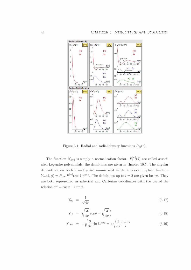
Graphical representations of R as a function of distance r are given in Fig. 3.1
together with the radial density function 4π2r2R2nl which represents the probability
of finding an electron in the radial direction.
44 CHAPTER 3. STRUCTURE AND SYMMETRY
Figure 3.1: Radial and radial density functions Rnl(r).
The function Nl|m| is simply a normalization factor. P|m|l (θ) are called associ-
ated Legendre polynomials, the definitions are given in chapter 10.5. The angular
dependence on both θ and φ are summarized in the spherical Laplace function
Ylm(θ, φ) = Nl|m|P|m|l (cos θ)eimφ. The definitions up to l = 2 are given below. They
are both represented as spherical and Cartesian coordinates with the use of the
relation eix = cosx+ i sin x.
Y00 =1√4π
(3.17)
Y10 =
√
3
4πcos θ =
√
3
4π
z
r(3.18)
Y1±1 = ∓√
3
8πsin θe±iφ = ∓
√
3
8π
x± iy
r(3.19)

3.1. QUANTUM MECHANICS OF THE HYDROGEN ATOM 45
Y20 =
√
5
16π(3 cos2 θ − 1) =
√
5
16π
3z2 − r2
r2(3.20)
Y2±1 = ∓√
15
8πsin θ cos θe±iφ = ∓
√
15
8π
(x± iy)z
r2(3.21)
Y2±2 =
√
15
32πsin2 θe±2iφ =
√
15
32π
(
x± iy
r
)2
(3.22)
Now we want to express a spatial representation of the wave functions. For
that the complex functions are a problem. But one result of quantum mechanics
is that for functions with the same energy eigenvalue (Ylm are l-fold degenerate)
a linear combination of degenerate functions are also solutions to the Schrodinger
equation. Therefore subtraction and/or addition of two functions will eliminate the
imaginary or real component. An example is to be calculated in the questions of
recapitulation. In a short notation the wave functions get indices consisting of the
principal quantum number n, a small letter for the orbital quantum number l being
s, p, d, f, g, h, . . . for l = 0, 1, 2, 3, 4, 5, . . . and the coordinates the wave function
depends on. For l = 0 we get only one wave function, for l = 1 there are three for
the three coordinates x, y, and z. For l = 2 we obtain five and for l = 3 seven wave
functions. Up to n = 3 the wave functions are given as
ψ1s =
√
1
4πR10 (3.23)
ψ2px =
√
3
4πR21
x
r(3.24)
ψ2py =
√
3
4πR21
y
r(3.25)
ψ2pz =
√
3
4πR21
z
r(3.26)
ψ3dz2
=
√
5
4πR30
3z2 − r2
2r2(3.27)
ψ3dxz =
√
15
4πR31
xz
r2(3.28)
ψ3dyz =
√
15
4πR31
yz
r2(3.29)
ψ3dx2−y2 =
√
15
4πR32
x2 − y2
2r2(3.30)

46 CHAPTER 3. STRUCTURE AND SYMMETRY
ψ3dxy =
√
5
4πR32
xy
r2(3.31)
With these descriptions of the wavefunctions we can generate a 3-dimensional
representation of the so-called electron orbitals. While for the spherical s-orbitals
this can be easily done including the representation of nodes changing the sign of
the wave function with different colors (see Fig. 3.2), this becomes nearly impossible
for p- and d-orbitals.
Figure 3.2: Graphical representation of 1s and 2s orbitals.
A more simple way is to present the wavefunctions by drawing orbitals repre-
senting a 90% probability that the electron is inside this area. In this way 2p and 3d
orbitals can be represented as shown in Fig. 3.3. Two-dimensional representations
are also possible in this way. A change in sign of the wavefunction is indicated by
+ and - or shades in different color. One has to keep in mind though that there is
a 10% probability that the electron is outside the given space of the orbital.

3.2. MOLECULAR ORBITALS 47
Figure 3.3: Graphical representation of 2p and 3d orbitals.
For a better demonstration, a visualization program for orbitals can be down-
loaded for instance at http://www.orbitals.com/orb/ov.htm.
The solutions to the Schrodinger equation are strictly valid only for the hydrogen
atom. For similar atoms, such as alkali atoms having a single electron in the outer
shell, only slight modifications have to be done as will be shown in chapter 3.3.
3.2 Molecular Orbitals
We consider the simplest molecule which is the hydrogen molecular ion H+2 since
it contains only one electron together with two nuclei. A full quantum-mechanical
treatment is only possible by the use of the Born-Oppenheimer approximation. This
tells us that the electron being so much lighter than the nuclei it will move consid-
erably faster than the nuclei which means that the internuclear distance R can be
fixed (for the ground state of a molecule this is clearly valid; one can assume that
in a given time a nucleus moves by 1 pm while at the same time the electron moves
1000 pm). With this approximation we can define the Hamilton operator for the
electron in the electric potential of two nuclei A and B:
H =h2
2me∇2 − e2
4πǫ0
(
1
rA+
1
rB
)
(3.32)
For the full description of the system, the nuclear repulsion has to be included
φrepulsive = +e2
4πǫ0R(3.33)
The Schrodinger equation can be exactly calculated and for a given value R the

48 CHAPTER 3. STRUCTURE AND SYMMETRY
energy eigenvalues are obtained. Combining these we obtain the potential curve in
this system as exemplified in Fig. 3.4.
Figure 3.4: Potential curve of diatomic molecules. De denotes the dissociation
energy and re the equilibrium distance.
Any further molecule is not anymore exactly calculable. Therefore we will adapt
a scheme that is rather simple and good for qualitative results. Let’s assume in
the H+2 molecule that the electron is near nucleus A. Then we can disregard the
potential from nucleus B since rA ≪ rB or 1rA
≫ 1rB
. The opposite is true if the
electron is near nucleus B. Therefore we can describe the resulting wave function as
a combination of two atomic orbitals
ψ = N [ψ1s(A) + ψ1s(B)] (3.34)
ψ2 = N2[ψ21s(A) + ψ2
1s(B) + 2ψ1s(A)ψ1s(B)] (3.35)
N is the normalization factor to ensure that∫
ψ2dτ = 1. The term
S =∫
ψ1s(A)ψ1s(B)dτ (3.36)
is called the overlap integral and indicates an increased electron density between the
two nuclei.

3.2. MOLECULAR ORBITALS 49
The methodology we applied here is known as Linear Combination of Atomic
Oorbitals or LCAO method (sometimes named as LCAO-MO, the latter for Molecular
Orbital). The resulting function is called a bonding orbital and in this case due to
the rotational symmetry about the internuclear axis it is called a σ orbital (see Fig.
3.5).
In a similar way the subtraction of the two atomic orbitals results in an anti-
bonding orbital:
ψ = N [ψ1s(A) − ψ1s(B)] (3.37)
ψ2 = N2[ψ21s(A) + ψ2
1s(B) − 2ψ1s(A)ψ1s(B)] (3.38)
The last term reduces the electron density between the nuclei. The antibonding
orbital is indicated by an asterisk, in this case a σ∗ orbital.
In a similar manner we can create molecular orbitals from other atomic orbitals.
For the three p-orbitals two different types of molecular orbitals are created. By
definition the z-direction points along the internuclear vector. A combination of
two pz orbitals therefore also yields a σ orbital while combination of two px or two
py orbitals will generate π orbitals with a node through the internuclear axis. The
graphical representation is also included in Fig. 3.5. Clearly, a combination of a px
and a py orbital cannot generate a bonding orbital.
Depending on the energy values of the individual atomic orbitals also other
combination of orbitals are possible, e. g., combination of an s and a pz orbital or
of a px and a dxy orbital. With d atomic orbitals we can also generate δ molecular
orbitals. Finally, there can be also non-bonding orbitals existing though they have
no influence on the total energy of the molecule.
Figure 3.5: Bonding and antibonding molecular orbitals of H+2 .
In a traditional MO scheme the molecular orbitals are filled from bottom to

50 CHAPTER 3. STRUCTURE AND SYMMETRY
top with maximum two electrons per orbital with opposite spin (see chapter 3.3).
Another practical rule is that N atomic orbitals will create N molecular orbitals.
With that it can clearly be seen that the H2 molecule is energetically more stable
than two individual hydrogen atoms (Fig. 3.6). Consequently, a molecule such as
He2 will not exist (an antibonding orbital is always slightly more antibonding than
a bonding orbital bonding). Nevertheless, a He+2 molecule should be able to exist
and was also experimentally observed.
Figure 3.6: MO-scheme of H2.
Finally, consider the different MO schemes of N2 and O2 (Fig. 3.7).
Figure 3.7: MO-scheme of N2 (left) and O2 (right).
3.3. MULTI-ELECTRON SYSTEMS, TERM SYMBOL 51
For O2 the procedure is straightforward with the restriction that degenerate or-
bitals (2π∗) are first filled with one electron only. This way it is easy to demonstrate
why the oxygen molecule is paramagnetic. The situation is different for the nitrogen
molecule. The order of the orbitals is reversed between 2pπ and 2pσ orbitals. This
is because we have to take into account overlap of 2s and 2p orbitals. This is more
relevant for lighter atoms because of smaller shielding effects (see chapter 3.3). The
energy separation between 2s and 2p orbitals increases along the period. Therefore,
for nitrogen (and lighter possible molecules in the 2nd period) we have to consider a
more complex LCAO wave function:
ψ = c2sψ2s(A) + c2pzψ2pz(A) + c2sψ2s(B) + c2pzψ2pz(B) (3.39)
This is indicated in the MO diagram by dotted lines. The resulting 2sσ∗ and 2pσ
orbitals spread apart from each other (because of symmetry reasons) and therefore
the 2pπ orbital is the energetically lowest 2p MO.
3.3 Multi-Electron Systems, Term Symbol
For the systems we discussed in the previous chapters, a limited number of electrons
were present that enabled a general description of the energy levels. We will now
develop a more generalized way to define the energy ground state without the exact
quantum mechanic description.
Similar to the classical energy values for the hydrogen atom this can be simply
transferred to the quantum mechanic result
Enlm = −hc0RH
n2(3.40)
The energy values - to first order - only depend on the principal quantum number
n. The quantum numbers are related by the inequality
|m| ≤ l ≤ n− 1 (3.41)
For transitions between the different energy levels the following selection rules
apply:
∆l = ±1 (3.42)
∆m = 0,±1 (3.43)

52 CHAPTER 3. STRUCTURE AND SYMMETRY
There are no restrictions for changes to the principal quantum number n.
The first rule can simply be explained from the conservation of angular momen-
tum by taking into account that a photon has spin 1; this means that emission
or absorption - meaning creation or destruction of a photon - changes the orbital
quantum number by one.
The selection rules can be used to describe the spectral transitions in an alkali
atom - this case sodium (Fig. 3.8). In a simplified picture we only consider the
outermost single electron which is often named valence electron. The inner electrons
are taken into account by their shielding effect since they shield the valence electron
from the electric field of the nucleus. It is easy to see that for electrons in an s-
orbital that according to the radial wave function have a non-zero charge density at
the position of the nucleus (see chapter 3.1) the shielding is ineffective. Furthermore,
for electrons in p- and d-orbitals the most probable position of charge move further
away from the nucleus. Therefore the shielding effect of inner electrons is more
effective for those. Combining these considerations one can correct the energies of
the different transitions, however we will just mention the qualitative effects.
Figure 3.8: Energetic transitions for the sodium atom.
Historically, for the different values of the orbital quantum number l the letters s,
p, d, f for l = 0, 1, 2, 3 are used which are abbreviations of sharp, principal, diffuse,
and fundamental. For larger values of l these are given the characters in alphabetical

3.3. MULTI-ELECTRON SYSTEMS, TERM SYMBOL 53
order g, h, i, k, .... For multi-electron systems, the orbital quantum numbers l of the
individual electrons is combined to a total orbital quantum number L. Therefore
the states are labeled S, P,D, F, ... in the same way as for single electrons.
The fourth quantum number is dedicated to the spin of the electron which is
related to an intrinsic angular momentum (also nuclei can have spin). Stern and
Gerlach showed in 1922 this phenomenon in their experiment. They used a beam of
silver atoms (having a single 5s electron) to lead through an inhomogenous magnetic
field. The force acting on the electron (~µ× ~B) lead to the occurrence of two spots
of silver instead of a continuum like expected classically. Later this was given the
expression of spin with values for a single electron of s = ±12. For multi-electron sys-
tem the individual spins are combined to a total spin S. Orbital angular momentum
and spin combine to the total angular momentum
~j = ~l + ~s (3.44)
From the selection rule ∆j = 0,±1 is follows that spin and orbital angular
momentum can only be parallel and antiparallel in orientation. For the principal
branch for the sodium atom (see above), we therefore obtain practically a doublet
for the sodium-D line because of the possible transitions between the S-state with
j = 12
and the P-state with j = 12
or j = 32.
To characterize multi-electron systems with all the spin, orbital, and total an-
gular momentum, the term symbol was created. The central point is the total
orbital quantum number expressed by the symbols S, P,D, F, .... On the top left
of this the spin multiplicity is given according to 2S + 1 to yield integer number.
On the lower right the total angular momentum is given, see the derivation below.
With this, one can characterize a multi-electron system with one simple expression.
For the sodium D-line example, we would have transitions between a 2S 12
and 2P 12
or 2P 32
states.
For multi-electron systems, a few rules exist how the electrons are distributed
on the different orbitals. The first rule applies to all orbitals and is called the Pauli-
principle after Wolfgang Pauli. In general it states, that two electrons cannot have
four identical quantum numbers. More applied it means that in an orbital (which
can fit maximum two electrons) with two electrons they have to have opposite spin.
Additionally, there are rules named after Friedrich Hund (practically there are
four rules, the first being that fully occupied shells with quantum number n have

54 CHAPTER 3. STRUCTURE AND SYMMETRY
a total angular momentum j = 0). One is that the term with maximum S has the
lowest energy and the other one that for the given S the one with the largest L has
lowest energy:
S = Max
(
∑
i
msi
)
(3.45)
L = Max
(
∑
i
mli
)
(3.46)
The maximum number for S is easily obtained by first filling all orbitals with
one electron in parallel orientation before adding a second electron with antiparallel
spin into an orbital. For maximum L consider that for a given n and l, ml runs
from −l to +l. Then by first filling the electrons in the orbitals with larger ml the
value for L can be maximized. Nevertheless, it has to be kept in mind that first the
maximum value of S has to be obtained before maximizing L.
Finally, the total angular momentum can principally obtain values between J =
|L−S| . . . L+S. The ground state or lowest energy has the one with J = |L−S| if
the shells are less than half full and J = L+S for shells that are more than half full
(for half full shells J = S). The reason behind this can be explained in a way that
spin and orbital angular momentum want to be antiparallel to each other (orbiting
negative electron charge creates a magnetic field) which explains the value for less
than half full shells. In the other case the missing necessary electron to fill the shell
completely can be understood as ’holes’ that creating an opposite magnetic field
and therefore a parallel arrangement of L and S is energetically favored.
Remember that these rules apply to find the energetic ground state of a multi-
electron system. All other combinations are possible, just require higher energy. In
the ’Questions of Recapitulation’ there are a few examples given to determine the
energetic ground state of certain atoms. If there is more than one unoccupied shell,
the value for J is determined by the relation of the total number of electron to the
total number of available electrons. Based on the term symbol the top left number
for 2S + 1 is referred to a singlet, doublet, triplet, quartet, ... energetic state for
values of 1, 2, 3, 4, ...

3.3. MULTI-ELECTRON SYSTEMS, TERM SYMBOL 55
Spin-Orbit Interaction
So far, we neglected interaction of the spin momentum and angular orbital mo-
mentum of an electron. Though if one takes into account coulomb interaction and
magnetic interaction of electrons, it becomes clear that such an interaction can be
significant.
Remember that a moving charge generates a magnetic field (just as in classical
electrodynamics). Then an electron with spin angular momentum has a magnetic
moment (spin) as well as the circulating current generated by the electron in an
orbital surrounding the nucleus has a magnetic moment (orbital momentum). The
interaction between these two magnetic moments is called spin-orbit interaction.
The combination of the two will create a total angular momentum as the vector
sum of the two momenta (further details will be given in chapter 5).
As can be easily understood, the spin-orbit coupling depends on the nuclear
charge, the higher the charge the larger the current and therefore the larger the spin-
orbit coupling (the spin magnetic moment interacts with the orbital magnetic field).
In practice, the interaction scales with ∝ Z4 (Z: atomic number). For example, for
a given system, for the hydrogen atom the coupling is 0,4 cm−1, whereas for lead it
is on the order of 1000 cm−1!
With this information, two general scenarios have to be differentiated: In case
of small spin-orbit interaction (mainly for light atoms), we speak of LS- or Russell-
Saunders-coupling. Here, the spin momenta si of the different electrons combine to
a total spin S as well as the individual orbital momenta li to a total angular mo-
mentum L. L and S then are used to calculate the total angular momentum J . On
the other hand for large spin-orbit interaction (mainly for heavy atoms), spin and
orbital momentum of each electron combine to a total angular momentum j = l+ s
which then are used to calculate the total angular momentum J =∑
ji. This type
is therefore called jj-coupling. The term symbol defined above is in principle for
LS-coupling, though it often can still be used even for heavy atoms.
In a similar way to the term symbol for atoms one can define a symbol for
molecules. Nevertheless it can become complicated to define this term symbol for
arbitrary molecules. Therefore we will introduce the molecular term symbol for
linear molecules where the internuclear axis is significant for space quantization.

56 CHAPTER 3. STRUCTURE AND SYMMETRY
It has the general form:2S+1Λ
(+/−)Ω,(g/u) (3.47)
with the notations
• S is the total spin quantum number, identical to the atomic term symbol
• Λ is the similar expression related to L for the atom expressed with greek
letters (Σ,Π,∆,Φ, . . .). A new quantum number λ = |ml| is defined for a
given molecular orbital. With that, Λ = |Ml| = |∑iml,i|. Keep in mind, that
due to the degeneracy for a linear molecule (λ and Λ defined from the absolute
values), there are twice as many degenerate states if Λ 6= 0.
• Ω is related to the total angular momentum of the molecule, Ω = Λ + Σ
• u/g is defined with respect to the presence of an inversion point. If the wave
function is unchanged due to a center of inversion, it is name g (from the
german ’gerade’, meaning even). If the wave function is changed it is named
u (german ’ungerade’, odd).
• +/- is defined with respect to the presence of an arbitrary mirror plane contain-
ing the internuclear axis, similar to u/g, + meaning symmetry, - antisymmetric
to the plane of reflection.
The definitions of u/g and +/- already lead to the next chapter dealing with the
symmetry of molecular and orbitals. Beforehand, we shall illustrate the molecular
term symbol by two examples:
The hydrogen molecule H2 is characterized by two electrons with opposite spin,
therefore S=0, a singlet state. Λ = 0 which results in a Σ term and Ω therefore is 0
as well. The molecular term symbol therefore is
1Σ0 (3.48)
The ground state of the oxygen molecule O2 was shown in Fig. 3.7. For the 1s
and 2s electron shells being complete these can be disregarded. Then we are left with
2 electrons in the 2pσ, 4 electrons in the 2pπ, and 2 electrons in the 2pπ∗ orbitals
(remember the two latter electrons being both with parallel spin in two different

3.4. GROUP THEORY 57
orbitals). Then we get 2S + 1 = 3 and Λ = 0. By looking at the orbital symmetry,
the 2pπ∗ orbital is a g term and we obtain for the molecular term symbol
3Σ−g (3.49)
The - comes from the antisymmetric behavior of the molecular orbital with re-
spect to a mirror plane including the internuclear axis.
Using the molecular term symbol, the following selection rules for electronic
transitions apply:
∆Λ = 0,±1 (3.50)
∆S = 0, (3.51)
∆Ω = 0,±1 (3.52)
Σ+ ↔ Σ+ , Σ− ↔ Σ− (3.53)
g ↔ u (3.54)
The total spin quantum number is retained, as long as there is no (significant)
spin-orbit coupling.
3.4 Group Theory
While the quantum mechanical treatment of transitions is a correct way to determine
transition dipole moments and with that transition probabilities, a consideration of
symmetry arguments done in this chapter will at least determine if a transition is
allowed or forbidden and therefore yield qualitative results. Additionally, this pro-
cedure is much simpler.
Point Groups
The symmetry of molecules, orbitals or three-dimensional objects in general can
be described by certain symmetry operations that retain the original structure. For
a molecule, this could mean that certain atoms cannot be differentiated due to
symmetry reasons, e. g., in chloromethane (CHCl3) a rotation by 120 around the
C-Cl axis interchanges the different hydrogens.
Five different symmetry operations can be differentiated
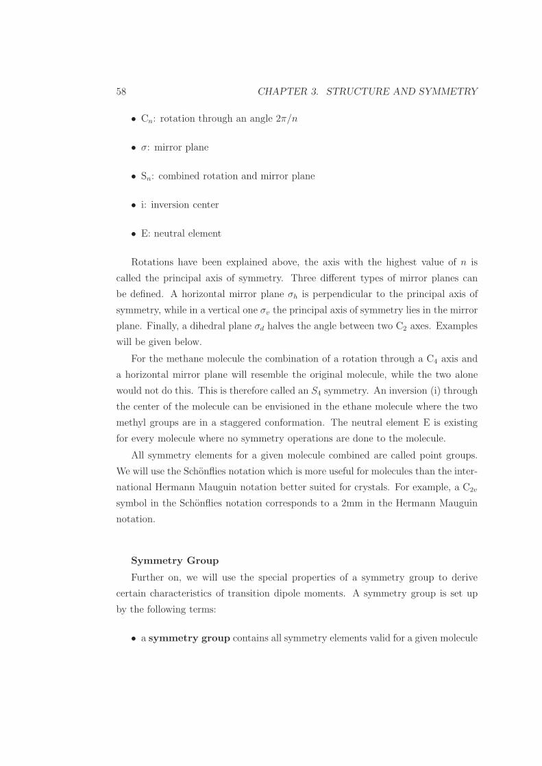
58 CHAPTER 3. STRUCTURE AND SYMMETRY
• Cn: rotation through an angle 2π/n
• σ: mirror plane
• Sn: combined rotation and mirror plane
• i: inversion center
• E: neutral element
Rotations have been explained above, the axis with the highest value of n is
called the principal axis of symmetry. Three different types of mirror planes can
be defined. A horizontal mirror plane σh is perpendicular to the principal axis of
symmetry, while in a vertical one σv the principal axis of symmetry lies in the mirror
plane. Finally, a dihedral plane σd halves the angle between two C2 axes. Examples
will be given below.
For the methane molecule the combination of a rotation through a C4 axis and
a horizontal mirror plane will resemble the original molecule, while the two alone
would not do this. This is therefore called an S4 symmetry. An inversion (i) through
the center of the molecule can be envisioned in the ethane molecule where the two
methyl groups are in a staggered conformation. The neutral element E is existing
for every molecule where no symmetry operations are done to the molecule.
All symmetry elements for a given molecule combined are called point groups.
We will use the Schonflies notation which is more useful for molecules than the inter-
national Hermann Mauguin notation better suited for crystals. For example, a C2v
symbol in the Schonflies notation corresponds to a 2mm in the Hermann Mauguin
notation.
Symmetry Group
Further on, we will use the special properties of a symmetry group to derive
certain characteristics of transition dipole moments. A symmetry group is set up
by the following terms:
• a symmetry group contains all symmetry elements valid for a given molecule

3.4. GROUP THEORY 59
Table 3.1: The character table for the group C2v.
C2v, 2mm E C2 σ(xz)v σ′(yz)v
A1 1 1 1 1 z z2, y2, x2
A2 1 1 -1 -1 Rz xy
B1 1 -1 1 -1 x, Ry xz
B2 1 -1 -1 1 y, Rx yz
• the number of elements in a symmetry group determines its order. For ex-
ample, if more than one C2 group exists, this is only counted once for the
order.
• derived from matrix considerations of symmetry operations, the character is
a number relating to the symmetry of an operation, being +1 for symmetric, -1
for antisymmetric, and 0, ±2 if it is degenerate. They derive from irreducible
matrix representations which will not be discussed here.
• the symmetry type is used to denote certain symmetry principles. These
are
– A, B: symmetric or antisymmetric with respect to Cn,max
– E, T: two- or threefold degeneracy
– 1, 2: symmetric or antisymmetric with respect to σv
– g, u: symmetric or antisymmetric with respect to i
To give more meaning to these definitions, consider the character table of the
point group C2v (Table 3.1), suitable for molecules such as H2O or SO2.
Character tables are always symmetric, i. e., for a given number of symmetry
elements the number of symmetry types has to be the same. The respective char-
acters can be comprehended according to the symmetry types and the symmetry
elements. For example, for symmetry type A2, the character for C2 has to be +1,
while for σ(xz)v it is -1. For this, the molecule is oriented in a way that the z-axis
is in parallel to the C2 axis and the molecule lies in the xz-plane.

60 CHAPTER 3. STRUCTURE AND SYMMETRY
Some general considerations about character tables: The symmetry type A1 or
Ag contains for every symmetry element the character +1. All symmetry types
have to be orthogonal to each other, i. e., multiplying the characters for a given
symmetry element and adding them together has to yield 0. The last two columns
in the character table contain geometric contributions. In the second to last column
elements for translation and rotation are given. The assignments can also be fol-
lowed by checking the corresponding characters for given symmetry elements. For
the notations x, y, and z one can also consider the geometry of the p-orbitals. This
column will later on be used to derive symmetry types that interact with the dipole
moment (see below). The last column will be used for interactions with the polar-
izability tensor (see below). As a hint, relation to the symmetry of d-orbitals help
for assignment to symmetry types. Orbitals reflecting the symmetry operations of
a given symmetry type are then labeled accordingly with small letters, e. g., a px-
orbital in the C2v group would be named a b1 orbital and so on.
There are numerous applications for character tables. Since we are interested in
the absorption and emission of electromagnetic radiation, we have to consider the
transition dipole moment (see chapter 2.6).
~M21 = q∫
ψ∗2~rψ1dτ (3.55)
with ~µ = q~r being the dipole moment. Application of group theory cannot
calculate the transition dipole moment, but can give information if the integral is
zero or non-zero. In the first case, the transition would be forbidden, otherwise
allowed. For most cases, this information is sufficient.
Allowed transitions are from those symmetry types were all characters are +1
(A1, Ag, A1g). For electronic transitions, with the help of the character table we
have to multiply the symmetry types of the orbitals before and after transition with
the corresponding mode of ~r, being x, y or z.
X(x1, x2, x3) ∗ Y (y1, y2, y3) ∗ Z(z1, z2, z3) = (x1y1z1, x2y2z2, x3y3z3) (3.56)
For the water molecule, a transition from an orbital a1 to b1 would be allowed if
the corresponding symmetry type for ~r would be of the type B1, which is fulfilled
for x-translation.

3.4. GROUP THEORY 61
For electronic transitions the following arguments can be obtained:
• the symmetry type of the total state is derived from the product of the sym-
metry types of the individual electrons
• the symmetry type of an electron is identical to the symmetry type of the
corresponding orbital
• only non-filled orbitals need to be considered
If the polarization tensor determines a possible transition (e. g., for Raman-
interactions), the dipole moment has to be replaced by the polarization tensor con-
taining mixed products xixj (see chapter 2.5). The corresponding tensor elements
can be ordered according to x2, y2, z2, xy, xz, yz, as is mentioned in the last col-
umn of the character table. These will be used further on to differentiate between
IR-active and Raman-active vibrations of a molecule where a change to the dipole
moment (IR) or the polarizability (Raman) is necessary.
To consider vibrations from multi-atomic molecules (diatomic molecules can only
have one vibration), we have 3N-6 possible vibrations with N being the number
of atoms. For linear molecules this reduces to 3N-5 since rotations around the
internuclear axis are not excited at normal temperatures due to the infinitely small
angular momentum (compare to classical mechanics). For CO2 we therefore would
have four vibrations that are illustrated in Fig. 3.9 together with the calculations
of the changes to the coordinates due to vibrations (internuclear axis is the z-axis,
y-axis points upwards).
The four vibrations are named symmetric, antisymmetric and two bending vibra-
tions. The factor c for the positional change of the carbon atom can be determined
from the masses of oxygen and carbon since the center of mass does not change
during a vibration
2βmO − cβmc = 0 ⇔ c = 2 ∗ 16
12=
8
3(3.57)
From these considerations, the symmetric vibration has the normal coordinate
α and the asymmetric the normal coordinate β. The two bending vibrations with
normal coordinates γ and θ are degenerate and therefore have the same angular
frequency.

62 CHAPTER 3. STRUCTURE AND SYMMETRY
Figure 3.9: Possible vibrations for CO2 together with the coordinates of the inidi-
vidual atoms labeled 1-3 according to their structure being O, C, O.
With the character table the corresponding integrals for IR (∫
ψ∗2xiψ1dτ) and
Raman transitions (∫
ψ∗2xixjψ1dτ) can be evaluated in accordance to the consid-
erations given above for electronic transitions. If the resulting symmetry type is
A1, Ag, A1g, the vibration is IR- or Raman active. A simplified rule states then that
for an IR-active vibrationdµ
dq6= 0 (3.58)
and for Raman-active vibrationsdα
dq6= 0 (3.59)
with q being the normal coordinate. In the character table, the dimension of the
vibrational subspace has to be calculated. It’s definition is as follows:
DimUi =hi
h
∑
k
hkTr(k)χi,k (3.60)
The definitions of the symbols are
• χi,k: value of the character table (i-th represenation, k-th class)
• hi: dimension of i-th representation (for A, B 1, for E 2, and for T 3)
• hk: order of the k-th class
• h =∑
k hk: order of the group
Tr(k) is most easily calculated from
Tr(k) = n(k) ∗ α(k) (3.61)

3.4. GROUP THEORY 63
Table 3.2: Values for α(k)
k E σ C2 C3 C4 C6 i S3 S4 S6
α(k) 3 1 -1 0 1 2 -3 -2 -1 0
Table 3.3: The character table for the group C2h.
C2h, 2/m E C2 i σh DimUi proper vibrations
Ag 1 1 1 1 Rz x2, y2, z2, xy 6 5
Bg 1 -1 1 -1 Rx, Ry xz, yz 3 1
Au 1 1 -1 -1 z 3 2
Bu 1 -1 -1 1 x, y 6 4
trace 18 0 0 6∑
= 18∑
= 12
with n(k) being the number of atoms that retain their position after a symmetry
operation and α(k) obtained from Table 3.2.
This complicated definition shall be analyzed by two examples. The first deals
with the molecule trans-dichloro ethylene. By considering the molecular geometry
one can identify the different symmetry elements that form the point group C2h. The
corresponding character table is illustrated in Table 3.3 that contains two additional
columns for our purpose of calculating the dimension as given above.
To start with, one can first calculate the trace for a given symmetry element.
This simplifies the calculation since one only needs to consider the characters for
the E and σh symmetry elements. For the calculation of the dimension than one
has hi ≡ 1 since there are only A and B terms present. For hk ≡ 1 and h ≡ 4.
From this, the corresponding dimensions are calculated. As a check, the sum of
all dimensions has to equal 3N for N the number of atoms. The last column, the
proper vibrations are then calculated by subtracting the rotations and vibrations
for a given symmetry type. The last step then involves the assignment of the Ag
and Bg types to Raman-active, and the Au and Bu types to IR-active vibrations
according to the occurrence of the corresponding elements in the sixth and seventh
column.
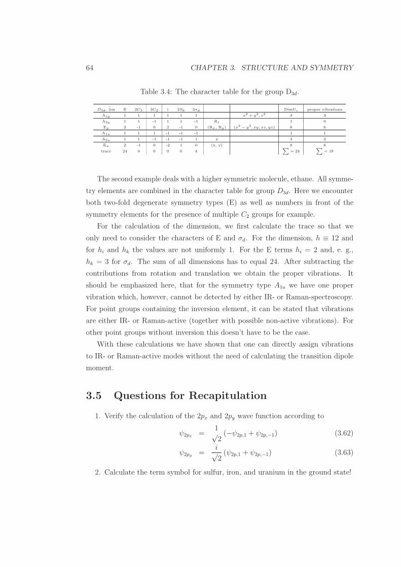
64 CHAPTER 3. STRUCTURE AND SYMMETRY
Table 3.4: The character table for the group D3d.
D3d,−
3m E 2C3 3C2 i 2S6 3σd DimUi proper vibrations
A1g 1 1 1 1 1 1 x2 + y2, z2 3 3
A2g 1 1 -1 1 1 -1 Rz 1 0
Eg 2 -1 0 2 -1 0 (Rx, Ry) (x2− y2, xy, xz, yz) 8 6
A1u 1 1 1 -1 -1 -1 1 1
A2u 1 1 -1 -1 -1 1 z 3 2
Eu 2 -1 0 -2 1 0 (x, y) 8 6
trace 24 0 0 0 0 4∑
= 24∑
= 18
The second example deals with a higher symmetric molecule, ethane. All symme-
try elements are combined in the character table for group D3d. Here we encounter
both two-fold degenerate symmetry types (E) as well as numbers in front of the
symmetry elements for the presence of multiple C2 groups for example.
For the calculation of the dimension, we first calculate the trace so that we
only need to consider the characters of E and σd. For the dimension, h ≡ 12 and
for hi and hk the values are not uniformly 1. For the E terms hi = 2 and, e. g.,
hk = 3 for σd. The sum of all dimensions has to equal 24. After subtracting the
contributions from rotation and translation we obtain the proper vibrations. It
should be emphasized here, that for the symmetry type A1u we have one proper
vibration which, however, cannot be detected by either IR- or Raman-spectroscopy.
For point groups containing the inversion element, it can be stated that vibrations
are either IR- or Raman-active (together with possible non-active vibrations). For
other point groups without inversion this doesn’t have to be the case.
With these calculations we have shown that one can directly assign vibrations
to IR- or Raman-active modes without the need of calculating the transition dipole
moment.
3.5 Questions for Recapitulation
1. Verify the calculation of the 2px and 2py wave function according to
ψ2px =1√2
(−ψ2p,1 + ψ2p,−1) (3.62)
ψ2py =i√2
(ψ2p,1 + ψ2p,−1) (3.63)
2. Calculate the term symbol for sulfur, iron, and uranium in the ground state!

3.6. REFERENCES 65
3. Calculate the IR- and Raman-active vibrations for the water molecule (point
group C2v!
3.6 References
general:
H. Haken, H. C. Wolf, Atom- und Quantenphysik, 8th ed., Springer 2004.
H. Haken, H. C. Wolf: Molekulphysik und Quantenchemie, 4th ed., 2003.
P. W. Atkins, Physical Chemistry, 6th ed., Oxford, 1999.

66 CHAPTER 3. STRUCTURE AND SYMMETRY

Chapter 4
Nuclear Magnetic Resonance
(NMR)
4.1 Introduction
1896 Pieter Zemann observed the splitting of optical lines in the presence of a mag-
netic field. Therefore, all splitting due to a magnetic field are referred to as the
’Zeeman effect’. In the megahertz and gigahertz range of the electromagnetic spec-
trum, these are related to energy splittings of nuclear spins or electron spins. The
latter, discovered 1944 by Jevgeni Konstantinovich Savoiski is called electron param-
agnetic resonance (EPR) or electron spin resonance (ESR), that will be the subject
in the next chapter. 1945 the groups of Edward Mills Purcell in Boston and of Felix
Bloch at Stanford did the first successful experiments on nuclear magnetic resonance
(NMR).
Nuclear magnetic resonance discussed here has to be differentiated from nuclear
resonance discussed in chapter 9. Nuclear resonance deals with transitions between
nuclear ground and excited states at very high frequencies of γ-rays and is experi-
mentally dealt with in Moßbauer spectroscopy.
4.2 Basics of NMR
In NMR, the subject of interest is the nuclear spin and transitions between nuclear
spin states. The spin quantum number I is related to the spin angular momentum
67

68 CHAPTER 4. NUCLEAR MAGNETIC RESONANCE (NMR)
by
|~L| = h√
I(I + 1) (4.1)
With the external magnetic field by definition oriented in the z-direction quan-
tization along this axis exists.
Lz = Izh ≡ mh (4.2)
with m being the magnetic quantum number which can take 2I + 1 values.
m = −I,−I + 1, . . . , I − 1, I (4.3)
The derivation of the spin quantum numbers for all isotopes is exactly only
possible with the help of nuclear physics. Nevertheless, three simple classifications
are useful:
• I is half-integer for odd mass numbers
• I is a whole number for even mass and odd proton numbers
• I is zero if both mass and proton numbers are even
From this, the properties of some common isotopes can be obtained. For in-
stance, 126 C, 16
8 O or 281 4Si have I = 0 and cannot be detected with NMR. More
common nuclei are 1H (I = 12), 13C (I = 1
2, natural abundance 1,1%), 14N (I = 1,
27Al (I = 52
or 31P (I = 12). For reasons that will become clear later, systems with
spin I = 12
can be treated simpler , since only two energy levels are involved and no
quadrupolar coupling is present.
In analogy to the classical description, a nucleus with spin creates a circular
current which produces a magnetic moment ~µ. This will create a torque in the
presence of an external magnetic field
~T = ~µ× ~B (4.4)
with the energy being defined as
E = −~µ · ~B (4.5)

4.2. BASICS OF NMR 69
The gyromagnetic (better: magnetogyric) ratio γ is a specific constant for each
isotope and is related to the magnetic moment via
~µ = γ~L (4.6)
with the z-component then being
µz = γLz = γIzh = γmh (4.7)
From this, the resulting energy (the energy difference to the case of absent mag-
netic field) is obtained
Em = −µzBo = −γmhB0 (4.8)
The magnetic field is generally defined as ~B = (0, 0, B0). In the case I = 12
we have
to two values m = ±12
and the energy difference is
∆E− 12, 12
= γhB0 = hωL (4.9)
This is illustrated in Figure 4.1.
Figure 4.1: Energy diagram for a spin-12
system.
ωL = γB0 is the Larmor-frequency that is the central equation of NMR. It states
that for every isotope we have a characteristic NMR frequency which makes NMR

70 CHAPTER 4. NUCLEAR MAGNETIC RESONANCE (NMR)
an element-selective detection technique. Additionally, the frequency is proportional
to the external magnetic field. Typical field strengths range from 2,4 to 24 T which
yield, e. g., for 1H frequencies between 100 and 1000 MHz.
While Iz is quantized, Ix and Iy are not. Therefore, all nuclear spins are arranged
oriented on a cone either in the direction of the magnetic field are opposing it
(orientation of m = ±12
depending on the sign of γ) precessing around it. For many
considerations it is advantageous to consider and calculate the sum of all nuclear
spins, the macroscopic magnetization M0. This can be calculated via
M0 = Nγh
∫m=+Im=−I me
γhmB0/(kT )
∫m=+Im=−I e
γhmB0/(kT )=Nγ2h2I(I + 1)
3kTB0 (4.10)
In the derivation the following sums are taken into account:∑
1 = 2I+1,∑
m = 0,∑
m2 = I(I+1)(2I+1)3
.
With M0 = χ0H0 = χ0B0
µ0(see chapter 2.1) this is directly related to the Curie
law χ0 = CT.
Spontaneous transitions can be neglected due to the low frequencies and prob-
abilities for absorption and induced emission are equal. Absorption or emissions
occurs if the two occupation numbers are different. To get an estimate of the sensi-
tivity of an NMR experiment, consider the Boltzmann distribution
N+ 12
N− 12
= ehγB0
kT = ehωLkT (4.11)
If the take for example ωL = 2π500MHz and T = 300K, we obatin for hωL
kT≈
8 · 10−5. Therefore the exponential function can be expanded to the linear term
(Taylor expansion, chapter 10.1) and we obtain for the difference in populations
N+ 12−N− 1
2
N− 12
=n
N− 12
≈ hωL
kT= 8 · 10−5 (4.12)
with n being the difference in occupation numbers. As this is a fairly small number,
NMR is practically a very insensitive measurement. Saturation can easily be reached
by the application of a continuous rf-field of the corresponding frequency. n can
be increased (apart from larger sample amounts) by lowering the temperature or
increasing the magnetic field.

4.3. EXPERIMENTAL SETUP 71
4.3 Experimental Setup
Though the setup of NMR spectrometers can vary, in general the following compo-
nents as given in Fig. 4.2 are generally present.
Figure 4.2: General components of an NMR spectrometer.
The critical point is the separation of pathways for the radio frequency going
to the NMR coil and the resulting induced voltage coming from the sample to be
collected. Since the ingoing power can be 6-8 orders of magnitude larger, an efficient
separation is necessary. Due to the low voltage as the response from the sample (on
the order of micro- to nanovolts), the signal is usually amplified before going to the
computer for analysis.
To differentiate are cw (continuous wave) and pulse spectrometers. In cw spec-
trometers the frequency (or magnetic field) are varied continuously. As this is time-
consuming, almost all spectrometers today are pulse spectrometers where a short
radio frequency (rf) pulse excites the whole spectrum at a time and then the in-
duced voltage is collected as a function of time, called free induction decay (FID).
The flip angle of a given pulse is defined as θ = tpω1 = tpγB1 with omega1 being
the radio frequency and B1 the radio frequency field. The corresponding pulses are
then named pi/2 or π-pulses.
4.4 Relaxation
Though not classically a spectroscopy, relaxation plays an important role in NMR.
Because of the Fourier pair time and frequency, a given relaxation time always refers

72 CHAPTER 4. NUCLEAR MAGNETIC RESONANCE (NMR)
to a frequency that can be correlated with the properties of matter. Therefore, we
will discuss the different relaxation times in NMR and how they are determined.
4.4.1 Spin-Lattice Relaxation
The spin-lattice relaxation T1, also longitudinal relaxation time, is the one related
to the lifetime of the excited state. The term longitudinal refers to orientation of
the macroscopic magnetization along the z-axis. If one considers disturbance of the
equilibrium magnetization, the regeneration of equilibrium follows the spin-lattice
relaxation. In this process energy has to be given away from the spin-system to
the outside (oscillations, rotations, translations, external fields) which is generally
called ’lattice’ (not to be confused with, e. g., the crystal lattice system).
For switching on or off of a magnetic field (rarely done in practice) the following
equations hold
n = n0
(
1 − e−tT1
)
(4.13)
n = n0e−tT1 (4.14)
(4.15)
with n denoting the difference in occupation numbers (n0 for equilibrium).
For the experimental determination of T1 we have to know that populations
cannot be determined directly with NMR. Observable magnetization is only that
which is oriented in the xy-plane so that a voltage can be picked up in the detection
coil. For this, mainly two pulse sequences are in use, Inversion Recovery (IR) and
Saturation Recovery (SR).
For the first (IR), a π pulse is applied to invert magnetization from the z to the -z
axis. After this, the system wants to regain equilibrium magnetization. In separate
experiments with variable delay after the π pulse, the magnetization is converted
to the xy-plane via a π2
pulse. Plotting the signal intensity (FID or spectrum) as a
function of this variable delay then yields the following curve (Fig. 4.3) that can be
fit using the equation
M(t) = M0
(
1 − 2e−tT1
)
(4.16)
A characteristic point is where the magnetization is zero, which directly yields
τ = T1 ln 2.

4.4. RELAXATION 73
! " # $ %
&%'
& '(
'
'(
%'
!"#
!"#$%&'
Figure 4.3: Signal intensity as a function of delay in the inversion recovery experi-
ment. The line is the fit using equation 4.16.
The saturation recovery sequence works in a similar way, but instead of the
π pulse it uses a set of π2
pulses with intermittent delays to effectively destroy z-
magnetization. The rest of the sequence is identical and the curves follows that of
the inversion recovery experiment from the point M(t) = 0. The fitting function
therefore is
M(t) = M0
(
1 − e−tT1
)
(4.17)
The choice of sequence is in principal arbitrary. Nevertheless, the saturation
recovery sequence is faster since one does not need to wait between consecutive
experiments (delay times) for the system to regain equilibrium which in principle
requires rough knowledge of the T1. On the other hand the inversion recovery is
more accurate since it spans a larger time scale.
4.4.2 Spin-Spin Relaxation
The induced signal or voltage in the detection coil decays with another relaxation
time constant, T2, the spin-spin relaxation or transverse relaxation time. Practically,
there is also a contribution from external magnetic field inhomogeneities that leads
to a faster decay. For this, the actual decay is often named T ∗2 with the ’real’ T2
being due to the sample with T ∗2 < T2.
Signal decay is a consequence of the loss of ’coherence’. This term documents
that after an initial π/2 pulses the phases of all nuclei are identical to the phase of the

74 CHAPTER 4. NUCLEAR MAGNETIC RESONANCE (NMR)
radio frequency pulse. After the pulse, interactions between the nuclei (see below)
leads to slightly different magnetic fields for the different nuclei and consequently
the phase relation is lost, called ’dephasing’.
To measure the spin-spin relaxation time, we usually can’t use the exponential
decay of the FID since it decays with T ∗2 . Two other possibilities can be used
instead (keeping in mind that for both experimental uncertainties still can lead to
smaller observed values). The first, is called ’Hahn-echo’, named after Erwin Hahn
developed in 1950 [].
In the Hahn-echo after a π2-pulse to transfer magnetization into the xy-plane
dephasing occurs during a period τ . This means that some spins precess at a higher
or lower frequency than the resonance frequency. Afterwards, a π-pulse inverts the
spins in the xy-plane. After another time τ all spins converge together at the same
point and form an ’echo’. An illustration is given by the ’Rennbahn-echo’ (Fig. 4.4).
Figure 4.4: Illustration of the Hahn-echo.
To determine the spin-lattice relaxation time, multiple experiments with differ-
ent echo times 2τ have to be run and the resulting curve fitted to a decreasing
exponential. A faster method is the CPMG-sequence (named after Carr-Purcell-
Meiboom-Gill) which produces repeat echoes by multiple π-pulses as illustrated in
Fig. 4.5. With this, the full curve can be observed within one experiment, though
spectroscopic resolution is lost.

4.4. RELAXATION 75
Figure 4.5: General CPMG-sequence.
4.4.3 Bloch Equations
Felix Bloch set up phenomenologically the effects of relaxation times T1 and T2 on
the magnetization. For this, he defined an effective magnetic field
Beff = (Brf , 0, B0 −ω
γ) (4.18)
Additionally, to the external static magnetic and radiofrequency field he added
the resonance offset ωL−ωγ
to include the effect when the radiofrequency deviates
slightly from the Larmor frequency. For the time dependence of the magnetization
we can the write
d ~M
dt= γ ~M × ~Beff −
Mx~ex +My~ey
T2− (Mz −M0)~ez
T1(4.19)
with T1 being effective on the z-component and T2 on the x- and y-component of
the magnetization.
In the stationary case (d ~M/dt = 0) we get the solution
Mx =(ω − ωL)T 2
2
1 + (ω − ωL)2T 22 + γ2B2
rfT1T2γBrfM0 (4.20)
My =T2
1 + (ω − ωL)2T 22 + γ2B2
rfT1T2γBrfM0 (4.21)
Mz =1 + (ω − ωL)T 2
2
1 + (ω − ωL)2T 22 + γ2B2
rfT1T2M0 (4.22)
These equation simplify if one uses weak rf-fields to prevent saturation. For this
case γ2B2rfT1T2 ≪ 1 and one obtains:
Mx =(ω − ωL)T 2
2
1 + (ω − ωL)2T 22
γBrfM0 (4.23)

76 CHAPTER 4. NUCLEAR MAGNETIC RESONANCE (NMR)
My =T2
1 + (ω − ωL)2T 22
γBrfM0 (4.24)
Mz = M0 (4.25)
4.4.4 Further Relaxation Times
In principle, further relaxation times can be defined. One more frequently used one
is called T1ρ or spin-lattice relaxation in the rotating frame. Here, one measures the
signal decay when radiofrequency pulses of different lengths are applied. The mag-
netization can be ’spinlocked’ along an axis in the xy-plane and decay is slower than
without the pulse. Nevertheless, because of the much higher external magnetic field
B0 finally the magnetization vector will orient along the z-axis again. Clearly, T1ρ
depends on the applied radiofrequency power and given values are of no information
content without this additional value.
In general, the study of relaxation times allows to determine frequencies of motion
of the material under study. Due to the direct relation between time and frequency
(Fourier pair) relaxation times are a direct measure of frequency. T1, T1ρ, and T2 can
span several orders of magnitude from microseonds to seconds and therefore enable
to probe different motions in frequency ranges from Hz to MHz.
The sources of relaxation are due to internal interactions within the material of
study which also have effects on the NMR spectrum that will be discussed in the
next section.
4.5 Interactions
This sections deals with the characteristic interactions in NMR spectroscopy that are
responsible for the resulting spectra. They also provide a mechanism for relaxation,
something that won’t be discussed here.
4.5.1 Chemical Shift
As mentioned in the previous chapter, the nucleus is shielded by the surrounding
electrons. This shielding is a result of an opposing current generated in the electrons.
4.5. INTERACTIONS 77
Therefore, the nucleus (or nuclear spin) experiences a slightly different magnetic field
from the external one.
Bloc = (1 − σ)B0 (4.26)
Because of the relation of the shielding to the chemical bonds, this interaction is
called chemical shift.
In fact σ is not a scalar constant but a tensor which is immediately apparent
from the fact that the orientation of a molecule with respect to the magnetic field
will produce anisotropic shielding effects (called chemical shift anisotropy, CSA). For
solution NMR, however, the Brownian motion averages all anisotropic effects and an
isotropic chemical shift remains. Historically, shielding effects are called diamagnetic
(from s-orbitals) and paramagnetic (from p- or other orbitals), though these terms
might be confusing since they can both be present in diamagnetic samples.
The absolute shielding values (with respect to the bare nucleus) can be calcu-
lated, but experimentally this is hard to perform. Therefore referencing with a
known substance is in use which accounts for the small differences due to the local
internal fields.
δ = σreference − σ (4.27)
For 1H, 13C, and 29Si the officially named reference compound is TMS (tetram-
ethylsilane). This also makes shift values given in ppm (parts per million) indepen-
dent of the magnetic field and allows for tabulation of shifts for numerous compounds
in databases. Since the chemical shift is a result from the electronic surrounding
of the nuclear spin, it is clear that this is a precise information for the assignment
of unknown structures. Typical shift values can directly be related to functional
groups. Even calculations predict values remarkably good (at least for solution
NMR). Therefore the determination of the chemical shift of a compound is of very
high importance.
The electron spin also influences the NMR frequency of a given nucleus. In dia-
magnetic samples due to pairing of electron spins due to the Pauli principle this
effect vanishes. Nevertheless in materials with lone electrons, like metals, supercon-
ductors, paramagnetic compounds, huge effects on the chemical shift are observed
which are referred to as Knight-shift. Prediction of Knight shifts is more compli-
cated and also shows a strong temperature dependence. Calculation of shifts is also
more complicated. Nevertheless, this interaction gives detailed information about

78 CHAPTER 4. NUCLEAR MAGNETIC RESONANCE (NMR)
the electronic structure. In solution NMR, sometimes paramagnetic salts are added
to detect resonances (spins, atoms) close to these salts as they show a remarkable
shift (’paramagnetic shift reagents’).
4.5.2 Indirect Dipolar Coupling
Next to the chemical shift, this interaction is the most important in solution NMR.
Besides the term indirect dipolar coupling also J-coupling or spin-spin coupling is
used. It derives from the fact that magnetic dipoles (nuclear spins) interact via
bonding electrons. Different couplings are illustrated by a symbol
nJAX (4.28)
Here, n denotes the number of chemical bonds between the coupling partners and
A and X denote the involved nuclei, e. g., HH or HC.
This interaction is independent of the external magnetic field, values for the split-
ting of the lines are usually given in Hertz [Hz]. Differentiation between signals from
chemical shift or spin-spin coupling is therefore possible via changing the magnetic
field. Equivalent nuclei don’t show a spin-spin coupling. If nuclei are equivalent can
be obtained from consideration of the symmetry of the molecule together with taking
into account free rotation of organic molecules about single bond (e. g., C-C bond).
There is a differentiation between chemical equivalence and magnetic equivalence.
The above described case means chemical equivalence. Magnetic equivalence exists
if nuclei that have the same chemical shift show only one spin-spin coupling to a
neighboring group.
For example, the 1Hs in difluoromethane, CH2F2, and those in the methyl group
of ethanol are equivalent. This is not the case for the 1Hs in 2,2’-difluoroethene,
C2H2F2, because the distances between the different nuclei are not the same.
To explain the observed splittings due to J-coupling we consider a 1JAX system.
We denote the m = +12
state by α and the m = −12
by β. Then, the αα state is
energetically lowest and ββ highest. The two mixed terms αβ and βα lie between
them and are only identical if a homonuclear system is considered. For an uncoupled
system, we obtain two lines since only transitions of one spin only can normally be
observed with NMR.

4.5. INTERACTIONS 79
For the illustration of the energy shifts due to J-coupling we have to consider the
corresponding electron spin involved in the chemical bond, see Fig. 4.6. The general
requirement is that the two electron spins - since belonging to the same orbital -
have to have opposite spin. A parallel orientation of electron and nuclear spin is
energetically preferred. For the αα system an antiparallel orientation leads to an
increase of the energy level (the same is true for the ββ system). For the mixed
systems, a parallel orientation of electron and nuclear spin can be fulfilled for both
nuclei, which leads to a reduction in energy. For the coupled system, this results in
an energy diagram shown in Fig. 4.7.
Figure 4.6: Illustration of J-coupling of two nuclei including electron spin orienta-
tion.
Together with the given transition energies, we obtain a doublet for each nucleus
with a separation of the spin-spin coupling constant J which is identical for the
coupled spins and therefore allows for assignments of coupled functional groups in
the NMR spectrum.
For a given number of equivalent coupled spins we then obtain doublets, triplets,
quartets, ... with the intensities according to Pascal’s triangle, shown in Fig. 4.8.
Clearly, if there are many different J couplings (even if they are only different
by 0.1 Hz), the coupling schemes can become very complicated. For quadrupolar
nuclei, Pascal’s triangle is not valid. For example, J-coupling to a 2H (I=1) yields
for one coupled 2H to a triplet with intensities 1:1:1 due to the three magnetic states
m=1, m=0, and m=-1.
So the combination of chemical shifts for identification of functional groups, the
indirect dipolar coupling identifies which functional groups are coupled to each other
and allow assignment of the arrangement of functional groups in the molecule.

80 CHAPTER 4. NUCLEAR MAGNETIC RESONANCE (NMR)
Figure 4.7: Energy levels and resulting NMR spectrum for uncoupled and coupled
system.
Figure 4.8: Pascal’s triangle.
4.5.3 Direct Dipolar Coupling
Next to the indirect dipolar coupling there is also a direct dipolar coupling which
involves to coupled dipoles that interact through space and no chemical bond is
required. One can easily understand that a magnetic dipole (a nucleus with mag-
netic moment) creates a small extra local magnetic field at a neighboring nucleus.
Therefore we obtain a slightly different resonance frequency
ω = γ(B0 +Blocalz ) (4.29)
4.5. INTERACTIONS 81
Mathematically, this frequency shift can be calculated as
∆ω ∝ ±γ1γ2h
r312
(3 cos2 θ − 1) (4.30)
There are different prefactors for differentiating homonuclear (γ1 = γ2) and
heteronuclear couplings (γ1 6= γ2). Important here is the inverse cube dependence
of the distance r between the spins which indicates that the size of the dipolar
couplings reduces rapidly with increasing distance and the angle θ which indicates
the angle between the external magnetic field and the internuclear vector.
The latter has many consequences: for a liquid sample with Brownian motion,
rapid tumbling of the molecules eliminates the direct dipolar coupling that doesn’t
show up the NMR spectrum. Mathematically, the dipolar coupling (as also the
chemical shift and principally the J-coupling) are tensorial interactions with the
dipolar coupling being a traceless tensor in opposition to the other two interactions).
In single-crystals, the splitting of the resonance line strongly depends on the angle
θ. By varying the orientation of the crystal with respect to the magnetic field this
interaction can be quantified and the distance between spins be determined very
exactly. In many solid samples, however, there is polycrystalline or even amorphous
material present with all different orientations θ. This leads to a characteristic
broadening of the line which can be calculated (’powder pattern’ or ’powder average’)
and the distance determined. Most prominent problem is the fact that all nuclei are
coupled with each other which soon complicates a spectrum beyond a point where
analysis is possible.
4.5.4 Quadrupolar Coupling
The discussion of quadrupolar coupling is often omitted since it is only present for
nuclei with a spin quantum number I > 12
and the fact that serious complications
to the NMR spectra are possible. We will therefore only briefly touch this aspect.
Due to a non-spherical charge distribution in the nucleus, for spins with I > 12
a quadrupolar moment results. This interacts with an electric field gradient that is
generated by the surrounding nuclei and electrons of neighboring atoms. An electric
field gradient (EFG) results if the symmetry around the spin of interest is non-
spherical, i. e., for exact octahedral or tetrahedral symmetry, no EFG is present.

82 CHAPTER 4. NUCLEAR MAGNETIC RESONANCE (NMR)
The electric field gradient can be obtained from the second derivative of the electric
potential
qij =∂2V
∂xi∂xj(4.31)
.
The quadrupolar interaction is also a traceless tensor so its effects don’t show
up in solution NMR. Characteristic value is the quadrupolar coupling constant
νQ =3e2Qqzz
2I(2I − 1)h(4.32)
which leads to a frequency splitting of
∆νQ =1
2νQ
[
3 cos2 θ − 1 − η sin2 θ cos 2φ]
(4.33)
η defines the asymmetry parameter
η =qyy − qxx
qzz
(4.34)
and indicates the deviation from axial symmetry of the EFG. θ and φ are defined
in a similar way as the spherical coordinates 10.4.
In a similar way to the dipole coupling, energy level shifts are obtained, see Fig.
4.9.
In the spin-52
system it can be seen that the central transition 12↔ −1
2is not
affected by quadrupolar coupling. This is only true as long as the quadrupolar
interaction is small with respect to the external magnetic field. This however, is not
always the case, coupling constants exceeding 20 MHz are known that also lead to a
shift of the frequency for the central transition. Mathematically this means that the
interaction cannot be treated as a small perturbation to the Zeeman interaction (1st
order perturbation theory), but as a larger one which requires 2nd order perturbation
theory. The details, however, are beyond the scope of this course.
4.6 Experimental Flexibility
Due the different interactions NMR spectra can become quite complicated and hard
to analyze. Nevertheless, the strength of the NMR technique is that due to variation
of the measurements certain interactions can be eliminated and therefore the analysis

4.6. EXPERIMENTAL FLEXIBILITY 83
Figure 4.9: Quadrupolar interaction energy levels and resulting spectra for a spin-1
and a spin-52
system.
simplified. Some examples will be discussed in this section. There are two principal
ideas, one is to do mechanical modifications and the other one is the use of a suitable
combination of pulses and delays (multipulse approach).
4.6.1 MAS
As was described for dipolar and quadrupolar coupling, there is an angular de-
pendence of the splitting. A similar effect is also existing for the chemical shift
anisotropy. All these interactions contain the angular term 3 cos2 θ− 1. By aligning

84 CHAPTER 4. NUCLEAR MAGNETIC RESONANCE (NMR)
a sample along an angle
arccos1√3≈ 54.74 (4.35)
this interaction should vanish. There is an additional requirement for sample rota-
tion (nowadays up to 70 kHz, driven by air flows) in order to align - in time average
- e. g. the internuclear vector along this so-called ’magic angle’.
If the spinning speed is high enough, chemical shift anisotropy (CSA), dipolar
coupling and 1st order quadrupole coupling can be eliminated. If the spinning speed
is not high enough, resolution improvement are still possible, just a number of
rotational (spinning) sidebands appear at multiple of the rotation frequency in the
spectrum, see example in Fig. 4.10. The envelope of the spinning sidebands contains
information about the corresponding interaction.
Figure 4.10: 13C static and MAS spectra of the carboxylic carbon of glycine.
4.6.2 Decoupling
A frequently used technique in NMR is spin decoupling. In a crowded J-coupled
spectrum the isotropic peaks cannot simply be assigned. By continuous irradiation

4.6. EXPERIMENTAL FLEXIBILITY 85
of a neighboring nucleus at its resonance frequency during detection removes the
coupling due to a permanent level transitions. This is often done for 13C detection
with 1H decoupling, but in principal can also be done between 1Hs of different fre-
quency though one has to be careful with the excitation bandwidth of the continuous
pulse. Both direct and indirect dipolar coupling are affected by decoupling.
4.6.3 Double Resonance
Double resonance in principle means the irradiation of two frequencies at the same
time. In a more strict sense, irradiation of two Larmor frequencies for two different
types of nuclei, e. g. 1H-13C, is meant. With this technique magnetization [co-
herence] transfer between the two spin systems is possible that can lead to signal
enhancement but can also be used to identify signals deriving from nuclei in close
proximity.
4.6.4 2D NMR
In general multidimensional NMR is a useful tool to separate NMR interactions
(e. g., J-couplings and isotropic chemical shifts) or to deduce connectivities between
signals that help in assignment of unknown structures.
Almost every 2D NMR pulse sequence can be separated into four phases:
preparation - evolution - mixing - detection
Evolution and detection are mainly time delays that are given the time variables
t1 and t2, respectively. These two time domains are later Fourier transformed in
the frequency axes F1 and F2, respectively. The detection is named the direct
dimension since in general an FID is recorded. For the indirect dimension (t1), a
stepwise increment is done between successive FIDs to simulate a time dimension
with a dwell time. In practice this leads to a modulation of the directly detected
FID. For preparation and mixing in the simplest case two π2
pulses are sufficient as
in the COSY (correlation spectroscopy) experiment.
The resulting 2D spectrum, shown in Fig. 4.11, contains diagonal elements for
magnetization that during t1 and t2 didn’t change its frequency and off-diagonal
elements indicating correlations since the frequency during t1 is different from that
during t2 because of a J-coupling interaction between the two coupled spins.

86 CHAPTER 4. NUCLEAR MAGNETIC RESONANCE (NMR)
Figure 4.11: Principal look of a H-H COSY experiment.
Many more combinations of pulses are possible, specifically designed for the
question of interest. In the same way as going from a 1D to a 2D experiment,
further dimensions can be created, though the time necessary for the measurement
increases significantly with every dimension.
4.6.5 Magnetic Resonance Imaging
Though practically not a spectroscopy, we nevertheless want to briefly introduce the
principles of magnetic resonance imaging which has a very high impact in medicine.
2D and 3D images of (parts of) the human body mainly reflect the density of
water in certain areas. Therefore, bones are represented as black elements. The main
idea of imaging is to have spatial resolution, i. e. a recorded frequency is directly
related to the position. For this, one has to create a well-defined inhomogenous

4.7. REFERENCES 87
magnetic field. This is done by external magnetic field gradients which is done by
gradient coils. If, for example, a gradient is given in x-direction, then the magnetic
field is given as
B(x) = B0 + x ∗G (4.36)
with G being the gradient strength. Because of ω = γB a given x-coordinate will
have a different frequency. This can in principal be done for all three dimensions
but practically there are also different gradients (phase gradients) used where the
phase of the signal indicates position for another direction. Then there are different
techniques existing to scan the 3D space more efficiently and faster which is more a
mathematical question of optimization.
The spin density image can be further modified by using contrasts like differences
in T1 and T2 relaxation times. Even the correlation between certain movements or
actions with activity in certain areas of the brain is possible (known as fMRI or
functional MRI). Here one uses the fact that hemoglobine present in the blood to
transport oxygen contains paramagnetic iron that influences strongly the relaxation
time. A high blood flow is then indicated by a strong decrease in relaxation time,
known as BOLD effect (blood oxygen level dependent). Many other useful applica-
tions of MRI such as quantifying blood flow in arteries show the importance of this
technique in modern medicine.
4.7 References
general:
M. H. Levitt, Spin Dynamics: Basics of Nuclear Magnetic Resonance, 2nd edition,
John Wiley & Sons, Hoboken, NJ, USA, 2008.
S. Braun, H.-O. Kalinowski, S. Berger, 150 and More Basic NMR Experiments,
Wiley-VCH, Weinheim, 1998.
H. Friebolin, Basic One- and Two-Dimensional NMR Spectroscopy, Wiley-VCH
Weinheim, 1993.
J. Keeler, Understanding NMR Spectroscopy, Wiley, 2005.
C. P. Slichter, Principles of Magnetic Resonance, Springer-Verlag, 1989.
M. T. Vlaardingerbroek, J. A. den Boer, Magnetic Resonance Imaging, Springer-
Verlag, 2002.

88 CHAPTER 4. NUCLEAR MAGNETIC RESONANCE (NMR)

Chapter 5
Electron Spin Resonance (ESR)
5.1 Introduction
Similar to NMR, electron spin resonance (ESR) - sometimes also named electron
paramagnetic resonance (EPR) - deals with the splitting of the electron spin states in
an external magnetic field. The first experiment was done 1944 by Jewgeni Sawoiski
at a magnetic field of 4.76 mT at a frequency of 133 MHz on a sample of copper(II)
chloride dihydrate. The existence of the electron spin was already demonstrated
before by the magnificent experiment by Stern and Gerlach (cf. chapter 3.3).
For ESR experiments to be possible, the existence of an atomic or molecular
magnetic moment is necessary. This requires the existence of unpaired electrons or
non-filled electron shells. For paired electrons due to the Pauli principle the two
electrons in an orbital have to have opposite spin and the moment is zero. This
limits the number of molecules and materials that can be investigated. These can
be categorized into
• free radicals, such as ·CH3
• transition metal ions with non-filled d or f orbitals
• defects in solids. Crystal imperfections might leave a point which contains just
an electron or other ways with a partially filled electron orbital
• ions with a non-bonding s-electron, such as Ga2+
89

90 CHAPTER 5. ELECTRON SPIN RESONANCE (ESR)
• systems with more than one unpaired electron, such as triplet states (e. g.
O2). These states can in principal also be generated via photoirradiation
• atoms with non-filled electron shells, such as atomic hydrogen or NO
• metals and semiconductors, which have unpaired electrons in the conduction
band
The major difference between NMR and ESR is the fact that the electron has
both spin and orbit and their interaction has to be taken into account. Therefore,
- in opposition to NMR - there is no direct relation between spin and resonance
frequency.
5.2 Experimental Setup
EPR spectrometers are mainly continuous-wave (cw) spectrometers. They work at
fixed frequencies that are named by characters and the magnetic field is varied. Typ-
ical frequencies are the X-band at 9.5 GHz and a magnetic field of 0.3 T, the Q-band
at 36 GHz and a magnetic field of 1.2 T, or the W-band at 95 GHz and a magnetic
field of 3.5 T. These magnetic fields are still quite low so that electromagnets can
be used. The frequencies are in the microwave range with wavelength on the order
of a few millimeter.
The typical setup of an ESR spectrometer is shown in Fig. 5.1.
The clystron is a frequency and power stabilized frequency synthesizer. Impor-
tant in the setup is the circulator which sends the power to the sample and the
reflected power from the sample to the detector. Transmittance of the microwave
frequency is done by waveguides that are rectangular tubes with the diameter equal
to the wavelength of the microwave. The other equipment is similar to the NMR
setup.
The magnetic field is swept linearly according to the formula
B0 = Binitial + const ∗ t (5.1)
Additionally, the magnetic field is modulated by a frequency of typically 100 kHz
that is generated by additional coils around the resonator. With that the magnetic

5.2. EXPERIMENTAL SETUP 91
Figure 5.1: Schematic setup of an ESR spectrometer.
field can be described as
B0 = Binitial + const ∗ t+Bmodulation ∗ sin(2πνmodulation ∗ t) (5.2)
The modulation frequency should be smaller than the EPR linewidth to prevent
falsification but also as large as possible to improve the signal-to-noise ratio. Due to
the limited bandwidth of the modulation a signal-to-noise gain is obtained compared
to the unmodulated signal. The modulated signal is afterwards demodulated before
computer display.
In opposition to NMR, ESR spectra are usually shown in dispersion mode (first
derivative of the absorption). By this, structures are easier to recognize as demon-
strated in figure 5.2 on the cost of quantitativeness. For the fact that absorption
spectra are more common to us, we will only display absorption spectra below.
For pulsed EPR, similar requirements exist as for pulsed NMR. Complications
are the broad spectra which complicate full excitation of the spectrum. That means
for a 100 MHz linewidth one needs pulses on the order of 10 ns. Additionally, since
spin-spin relaxation times are faster than in NMR, resonators with short dead times
are needed to record FIDs and echo times for spin echo measurements have to be
short. For these reasons, pulse sequences from NMR have to be adapted to ESR and

92 CHAPTER 5. ELECTRON SPIN RESONANCE (ESR)
Figure 5.2: Differentiation of absorption and dispersion spectra.
cannot be directly used. For relaxation time measurements, clearly, pulsed EPR is
needed.
5.3 g-Factor
To describe the for ESR very important g-factor, we have to consider both spin and
orbit of the electron. An orbiting electron at radius r with an angular frequency
ω creates a current I = −eω/(2π). The magnetic moment is then ~µ = I ~A with ~A
being the enclosed surface being A = πr2. Then we obtain
~µL = − e
2me
~L (5.3)
with L = mer2ω being the angular momentum.
In a similar way we can define the spin magnetic moment for a rotating sphere
of mass me and charge −e.~µS = − e
2me
~S (5.4)
where S is the electron spin.

5.3. G-FACTOR 93
L and S are both quantized
|~L| = h√
l(l + 1) (5.5)
|~S| = h√
s(s+ 1) (5.6)
The components along the external magnetic field (by definition along the z-axis)
are then
Lz = lzh ≡ mlh ≡ mh (5.7)
ml ≡ m = −l,−l + 1, . . . , l − 1, l (5.8)
Sz = msh ≡ sh (5.9)
ms ≡ s = −1
2,+
1
2(5.10)
The Bohr magneton is defined as a combination of different constants that come
across the previous definitions
µB = − e
2me
h = 9.274 · 10−24Jm2V −1s−1 (5.11)
With that, the magnetic moment can be expressed as
|~µ| = gµB
√
m(m+ 1) (5.12)
For orbital magnetism we obtain gL = 1. For the electron spin this is not as
simple and requires a relativistic quantum mechanical description. With that one
obtains that for the free electron g = 2.002319304386.
The total magnetic moment can be obtained from the consideration of Russel
Saunders coupling ~J = ~L + ~S. Though µL and µS are parallel to their angular
momenta, this does not need to be the case for ~MJ and ~J , as can be seen in Figure
5.3.
The resulting magnetic moments can then be expressed as
|~µL| = gLµB
√
L(L+ 1) (5.13)
|~µS| = geµB
√
S(S + 1) (5.14)
|~µJ | = gJµB
√
J(J + 1) (5.15)
In opposition to NMR, where the chemical shift is only a small change to the
resonance frequency (values given in ppm), the ESR analogue, the g-factor, results
in huge differences to the resonance frequency. General sizes of ESR interactions
will be given in chapter 5.6.

94 CHAPTER 5. ELECTRON SPIN RESONANCE (ESR)
Figure 5.3: Vector diagram for orbital and electron spin.
5.4 Zero Field Splitting
An interaction similar to the quadrupolar interaction in NMR exists also in ESR.
Since it is also present without magnetic field, it’s called zero field splitting (ZFS).
[Quadrupolar interaction known from NMR is also present without magnetic field
and can be studied by NQR - nuclear quadrupole resonance]
Consider a Cr3+ ion which has three electrons in the 3d shell which are located in
three different orbitals. The term symbol therefore is 4F 32, so there is a 7-fold degen-
eracy of the orbital momentum and 4-fold degeneration of spin. Due to interaction
of the d electrons with the electric field of the surrounding ions, for an octahedral
ligand field a splitting of the 4F 32
ground state into the point groups 4A2g,4T2g,
and 4T1g, see Fig. 5.4.
In the case of lower symmetry, e. g., axial symmetry (tetragonal), the 4-fold spin
degenerated 4A2g state splits up into two states with MS = ±12
and MS = ±32
with
an energy difference δ. The remaining 2-fold degeneracy is lifted by an external
magnetic field which results in three lines in the ESR spectrum. Without zero field
splitting all energy levels would be equally spaced and only one line would result.
The three-line spectrum is also referred to as fine structure therefore the zero-field
splitting is sometimes also called fine splitting.
Similar to NMR, the zero-field splitting is also orientation dependent so that in

5.5. HYPERFINE SPLITTING 95
Figure 5.4: Illustration of zero field splitting for a Cr3+ ground state.
solids like single-crystals, the anisotropic nature of the interaction becomes apparent
and can be analyzed by recording spectra at different orientations of a single-crystal
with respect to the external magnetic field.
5.5 Hyperfine splitting
The hyperfine splitting considers the interaction between the electron and a nucleus
with spin. Compared to NMR this is similar to a heteronuclear dipolar interaction.
It originates from Fermi contact interaction of the s-orbital density (which has a
non-zero probability of being at the nucleus) at the nucleus. This interaction has
also an anisotropic nature to be identified in solid-state EPR when also p-electrons
are involved.
The explanation of hyperfine splitting is that the nuclear spin creates a local

96 CHAPTER 5. ELECTRON SPIN RESONANCE (ESR)
field at the location of the electron.
BLocal = B0 + amI (5.16)
with a being the hyperfine coupling constant. For a nuclear spin I = 12, the energy
scheme in Fig. 5.5 results in an EPR spectrum with two signals split by a.
Figure 5.5: Energy diagram for hyperfine splitting of an electron with a nuclear spin
I = 12.
Similar to NMR, multiple coupling schemes result for several nuclei and also for
nuclear spins with I > 12.
The hyperfine splitting represents an important interaction in EPR since it allows
for the localization of the electron. The term super hyper fine splitting exists for
electrons interacting with the nuclear spin of a neighboring atom.
Clearly, there is also electron-electron dipolar interaction. For these, however, we
would require two lone electrons that interact without recombination. In an organic
molecule with radical at the two ends of the molecule, one could however determine
the distance of the electrons and with that for example the size of the molecule.

5.6. HAMILTON OPERATORS 97
5.6 Hamilton operators
In this section we briefly describe the principle Hamilton operators of the different
interactions in EPR that should only represent in general what the quantum me-
chanical description looks lik. The focus is on the sizes of these interactions given
at the end.
• Zeeman interaction
HEZ =µB
h~B0
↔g ~S (5.17)
• Zero field splitting
HZFS = ~S↔
D ~S = D[S2Z − 1
3S(S + 1)] +
1
2E(S2
+ + S2−) (5.18)
The E term hasn’t been explained but stands for the anisotropy of the inter-
action. S+ and S− are called raising and lowering operators and are defined
as S± = Sx ± iSy.
• Dipole-dipole interaction
HDD = ~S1
↔
D ~S2 =1
r3
µ0
4πhg1g2µ
2B[ ~S1
~S2 −3
r2(~S1~r)(~S2~r)] (5.19)
Compared to the zero field splitting, here the spin operator of two different
electrons are considered.
• Hyperfine coupling
HHFI,aniso = ~S↔
T ~S (5.20)
It can be seen that the interactions all have a similar form and all contain tensors
in the description identifying the interaction as anisotropic. For solution EPR, some
significant simplifications exist similar to NMR.
In opposition to NMR, the sizes of these interactions are strongly different.
Whereas in NMR, the Zeeman interaction is by far the largest, in EPR the or-
bital energy and the splitting in the ligand field exceeds the others. This can be
seen in table 5.1.

98 CHAPTER 5. ELECTRON SPIN RESONANCE (ESR)
Table 5.1: Sizes of EPR interactions.
interaction order of magnitude [cm−1]
orbital energy > 104
energy splitting in ligand fields 102 − 104
spin-orbit coupling for selected atoms B: 10, C: 28, F: 271, Cl: 440, Br: 1842
electron-Zeeman transitions 0.3 (X-band), 1 (Q-band)
zero field splitting (triplet ground state) ≈ 1
hyperfine interaction < 10−1
Zeeman transitions of 1H @ 0.7 T 10−3
5.7 ENDOR
At the end, we want to discuss one special experiment that involves electron-nuclear
interaction and is able to simplify ESR spectra. It is called Electron Nuclear
DOuble Resonance and therefore combines EPR excitation and detection using mi-
crowave with nuclear spin irradiation using radio frequencies. It can be understood
as detecting NMR transitions via EPR frequencies with the advantage of higher sen-
sitivity compared to NMR but lower than a normal EPR spectrum. Nevertheless,
the resolution is higher than in a normal EPR spectrum.
To explain the ENDOR spectrum, consider Fig. 5.6. For EPR the selection rules
are ∆mS = ±1 (and ∆mI = 0). For nuclear spin transitions ∆mI = ±1. For the
EPR six lines result all split by the hyperfine interaction constant a.
For the ENDOR spectrum, one of the EPR transitions needs to be saturated by
a strong microwave field. In Fig. 5.6 this is the transition for mI = 12. Then a radio
frequency sweep on the nuclear side is performed which results in transitions when
frequencies ν+ and ν− are reached since the saturation is lifted due to a change of the
population of the different states. This difference in occupation numbers produces
microwave absorption which is detected and produces only two lines split apart by
twice the Larmor frequency. This clearly simplifies the EPR spectrum especially if
also other interactions are present at the same time.

5.8. REFERENCES 99
Figure 5.6: Energy diagram for the ENDOR experiment for an electron spin inter-
acting with a nuclear spin I = 52.
5.8 References
general:
A. Abragam, B. Bleaney, EPR of Transition Ions, Clarendon, Oxford, 1970.
A. Schweiger, Puls-Elektronenspinresonanz-Spektroskopie, Angew. Chem. 103
(1991) 223.
P. W. Atkins, Physical Chemistry, Oxford University Press, Oxford Melbourne
Tokyo, 1990.

100 CHAPTER 5. ELECTRON SPIN RESONANCE (ESR)

Chapter 6
Rotational and vibrational
spectroscopy
6.1 Rotational Spectroscopy
Rotational spectroscopy is also called microwave spectroscopy although for small
molecules optical methods are also applicable. Necessary requirement for absorp-
tion measurements of rotational transitions is the existence of a permanent dipole
moment. If this doesn’t exist, but an anisotropic polarizability perpendicular to the
axis of rotation, Raman scattering can be used.
Investigated are in principle only gaseous samples, so the applicability is limited.
Nevertheless important parameters can be derived.
6.1.1 Experimental Setup
A scheme of the experimental setup is shown in Fig. 6.1. Generation of microwaves
is done by klystrons or Gunn diodes. Low pressures of the gases are used to decrease
the amount of collisions and wave guides can be up to 1 m long for higher sensitivity.
Similar to ESR (Chapter 5), modulation fields are used that also give rise to the
Stark effect (see chapter 6.1.4 below).
101

102 CHAPTER 6. ROTATIONAL AND VIBRATIONAL SPECTROSCOPY
Figure 6.1: General scheme for measurement of rotational spectra.
6.1.2 Quantum Mechanical Description
The moment of inertia I = mrr2 (for a diatomic molecule) is central to the discussion
of rotational spectroscopy. The Hamilton operator can be written as
Hψ = − h2
2mrr2
∂2ψ
∂φ2= Eψ (6.1)
with φ being one of the spherical coordinates.
From this the differential equation
∂2ψ
∂φ2= −2IE
h2 ψ (6.2)
The eigenfunctions can be written as
ψJ =
√
1
2πeiJφ (6.3)
with
J = ±√
2IE
h= 0,±1,±2 (6.4)
being the rotational quantum number.
The energy values are
E =J2h2
2I(6.5)
This derivation from classical starting points is only almost complete, J2 has to
be replaces by J(J + 1). This is because the axis of rotation was arbitrarily fixed,
though many different axis perpendicular to the molecular axis are possible.

6.1. ROTATIONAL SPECTROSCOPY 103
We get
EJ = J(J + 1)h2
2I= hBJ(J + 1) (6.6)
with the rotation constant B defined as
B =h
4πI=
h
8π2I(6.7)
given in frequency units.
The constant B becomes apparent as half of the frequency difference in rotational
transitions. For this, consider the rotational transitions J − 1 → J and J → J + 1.
For the energy differences we obtain ∆EJ,J−1 = 2hBJ and ∆EJ+1,J = 2hB(J + 1).
In frequencies, the separation is Eh
= 2B.
In the energy diagram, Fig. 6.2, it is important to note that the separation of
the energy levels increases with increasing J.
For rotationally symmetric non-linear molecules, we can define a symmetric ten-
sor of inertia with characteristic values parallel to the axis of symmetry I‖ = Iz = IA
and perpendicular to the axis of symmetry I⊥ = Ix = Iy = IB. If IA > IB the rotor
is shaped like a pancake, like in C6H6, in the opposite case, IA < IB like a cigar, like
in CH3Cl.
The two spherical coordinates θ and φ describe the rotation of the molecule
around arbitrary axes. The then resulting energy values are
ERot =h2
2IB
[
J(J + 1) −K2]
+h2
2IAK2 (6.8)
with 0 ≤ K ≤ J . If K = 0 the axis of rotation is perpendicular to the molecular axis
of symmetry analogous to the derivation above. With K = J , J ≫ 1, the second
term is dominant and the axis of rotation is almost parallel to the axis of symmetry.
Selection rules are ∆J = ±1 and ∆K = 0. For Raman spectra ∆J = 0,±2.
For asymmetric rotors and also free inner molecular rotations one can give ex-
pressions with more quantum numbers, which we skip here. A question arises, if
rotational spectra of spherical molecules such as CH4, SiH4 or SF6 can be obtained.
Though the molecules have no dipolar moment, for the tetrahedral CH4 rotation
around the C3 axis can lead to centrifugal distortion changing three of the four C-H
bond lengths and thereby creating a small dipolar moment. For example for SiH4 at
4 bar pressure a dipole moment of µ = 2.7 · 10−35Cm was determined. For compar-
ison, CO has a dipole moment of µ = 3.74 · 10−31Cm. For octahedral SF6, however

104 CHAPTER 6. ROTATIONAL AND VIBRATIONAL SPECTROSCOPY
Figure 6.2: Energy levels of a linear rotor.
rotation around the C4 axis would change the four S-F bonds in the plane but in
the same way which still results in a dipole moment of 0.
6.1.3 Rigid and Non-Rigid Rotor
We will now explain the specifics of two examples of diatomic molecules and their
effects on the rotational spectra.

6.1. ROTATIONAL SPECTROSCOPY 105
• Rigid Rotor, HI Fig. 6.3 indicates the necessary symbols within the HI
molecule.
Figure 6.3: The diatomic rotator HI.
The axis of rotation is perpendicular to the bonding axis and passes through
the center of mass. The moment of inertia can be simply expressed as I =
r2emr, with mr being the reduced mass mr = m1m2
m1+m2.
Experimentally, the spectrum consists of equidistant lines separated by 2B =
384 GHz. From this we can determine the moment of inertia
I = mrr2e = 4.37 · 10−47kgm2 (6.9)
and together with the reduced mass (mass number of 127 for iodine, only one
isotope)
mr = 1.65 · 10−26kg (6.10)
the interatomic distance can be obtained
re =
√
I
mr= 1.63A (6.11)
Therefore, from the moment of inertia distances and valence angles can be
obtained if the isotopic composition is known or otherwise the isotopic compo-
sition can be obtained if the interatomic distances are known. For asymmetric

106 CHAPTER 6. ROTATIONAL AND VIBRATIONAL SPECTROSCOPY
molecules, three different moments of inertia can be obtained which result in
a number of distances and angles. With isotopic replacement (e. g., H with
D) the number of measured values can even be increased.
• Non-rigid rotor, HCl Interatomic distances can increase with increasing ro-
tational frequency due to centrifugal distortion. For rotational spectra, this
means that B gets smaller with increasing J. Varying interatomic distance can
be understand by a vibration frequency as
ωs = 2πνs =
√
k
mr(6.12)
with k being the force constant. With that the interatomic distance can be
expressed as
r = re + fa cosωst (6.13)
With centrifugal force and displacement force being equal
mrrω2rot = k(r − re) (6.14)
we obatain with the moment of inertia I = mrr2 and angular momentum
L = Iωrot = mrr2ωrot, the rotational energy is composed of a rigid part and
and elastic part
ERot =L2
2I− k(r − re)
2(6.15)
Going from the classical to the quantum-mechanic description, with r3 = r3e
and L2 → J(J + 1)h2 the energy is
ERot =h2J(J + 1)
2I− h4J2(J + 1)2
2I2r2ek
(6.16)
= BJ(J + 1) −DJ2(J + 1)2 (6.17)
where D describes the elastic strain constant due to centrifugal distortion.
With the relation above D can be expressed as
D =h3
4πI3ω2s
=4B3
ν2s
(6.18)
This means that a large moment of inertia (D ∝ 1I3 ) and/or a large vibrational
force constant (D ∝ 1ν2
s) lead to a small distortion.
For gaseous HCl the experimentally obtained values are 2B = 20.79cm−1 and
D = 0.00054cm−1.

6.1. ROTATIONAL SPECTROSCOPY 107
6.1.4 Stark Effect
The Stark effect, discovered 1913 by Johannes Stark describes the lifting of the
degeneration of energetic levels due to an external electrostatic field (in analogy to
the Zeeman effect in external magnetic fields). In rotational spectra, there is a linear
and a quadratic Stark effect where the energetic splitting of the lines is linearly or
quadratic dependent on the external field strength.
For the explanation of the Stark effect, consider Fig. 6.4. We can define an
effective dipole moment along the axis of rotation. The component perpendicular
to this axis is average out by quick molecular rotation. With | ~K| = Kh and | ~J | =√
J(J + 1)h we obtain
| ~mueff | = | ~mu| K√
J(J + 1)(6.19)
Figure 6.4: Orientation of µ with respect to J and E.
In the same sense, the alignment of ~J with the external field depends on the
magnetic quantum number MJ = −J, . . . ,+J and we can define a component ~µE as
|~µE| = |~µeff |MJ
√
J(J + 1)(6.20)
For the interaction energy we obtain
WJ,K,M = −~µeff~E = −µE KMJ
J(J + 1)(6.21)

108 CHAPTER 6. ROTATIONAL AND VIBRATIONAL SPECTROSCOPY
From W(J) - W(J-1) the linear Stark shift of rotational lines is
∆νlinear =µE
h
2KMJ
J(J2 − 1)(6.22)
From MJ we get 2J+1-fold splitting and the dipole moment µ can be determined if
K and MJ are known. Clearly, for linear molecules the linear Start effect does not
exist, since K = 0.
The quadratic Stark effect is more frequent than the linear one. External electric
fields cause polarization effects so that it is also existing if there is no permanent
dipole moment. For linear molecules the frequency shift is given without derivation
as
∆νquadratic =(
µE
h
)2 6M2J (8J2 − 3) − 8J2(J2 + 1)
2BJ(J2 − 1)(4J2 − 1)(4J2 − 9)(6.23)
6.1.5 Line Intensities
For the intensity of rotational lines, start with the Boltzmann distribution
Ni
N=
e−EikT
∑
i e−
EikT
(6.24)
The denominator contain the sum of states. With EJ = hBJ(J + 1) we obtain
∑
i
e−EikT =
∑
J
(2J + 1)e−EJkT =
kT
hB(6.25)
On the left side of the equation the summation is both over J and MJ whereas on
the right side only over J . For the Boltzmann distribution we then obtain
NJ
N= (2J + 1)
hB
kTe−
EJkT (6.26)
After differentiation with respect to J and setting the result to zero we obtain
for the rotational quantum number with the highest occupation (intensity)
J =
√
kT
2hB− 1
2(6.27)
Due to the competing effect of the exponential and the term (2J+1) the max-
imum intensity lies at medium rotational quantum numbers, see Fig. 6.5. Due to
the temperature dependence, it can also be used to determine the temperature in
the absorption cell.

6.2. VIBRATIONAL SPECTROSCOPY 109
Figure 6.5: Intensity distribution of rotational lines.
6.2 Vibrational Spectroscopy
6.2.1 Harmonic Oscillator
Classically, the vibration can be described similar to a spring in mechanics
F = −fx (6.28)
V =1
2fx2 (6.29)
Quantum mechanically, we can write
− h2
2m
∂2ψ
∂x2+
1
2fx2ψ = Eψ (6.30)
⇒ ∂2ψ
∂y2+ (ǫ− y2)ψ = 0 (6.31)
with the definitions
y =x 4√mf√h
(6.32)
ǫ =2E
h
√
m
f=
E12hω
(6.33)

110 CHAPTER 6. ROTATIONAL AND VIBRATIONAL SPECTROSCOPY
For a diatomic molecule, m is replaced by the reduced mass mr and x denotes
the deviation from the equilibrium distance x = r − re. The Schrodinger equation
can be solved with ψ = He−fracy22 which has solutions only for ǫ = 2v + 1 with
v being integer and denoting the vibrational quantum number. The corresponding
energy values are
Ev = (2v + 1)1
2hω (6.34)
The energy levels are equidistant, selection rule for vibronic transitions is ∆v = ±1.
A representation of the probability distribution for the different energy values is
given in Fig. 6.6.
Figure 6.6: Probability density of the vibrational energy levels for the harmonic
oscillator.
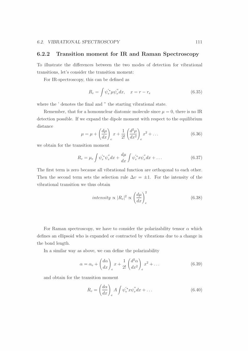
6.2. VIBRATIONAL SPECTROSCOPY 111
6.2.2 Transition moment for IR and Raman Spectroscopy
To illustrate the differences between the two modes of detection for vibrational
transitions, let’s consider the transition moment:
For IR-spectroscopy, this can be defined as
Rv =∫
ψ′∗v µψ
′′
vdx, x = r − re (6.35)
where the ’ denotes the final and ” the starting vibrational state.
Remember, that for a homonuclear diatomic molecule since µ = 0, there is no IR
detection possible. If we expand the dipole moment with respect to the equilibrium
distance
µ = µ+
(
dµ
dx
)
e
x+1
2!
(
d2µ
dx2
)
e
x2 + . . . (6.36)
we obtain for the transition moment
Rv = µe
∫
ψ′∗v ψ
′′
vdx+dµ
dx
∫
ψ′∗v xψ
′′
v dx+ . . . (6.37)
The first term is zero because all vibrational function are orthogonal to each other.
Then the second term sets the selection rule ∆v = ±1. For the intensity of the
vibrational transition we thus obtain
intensity ∝ |Rv|2 ∝(
dµ
dx
)2
e
(6.38)
For Raman spectroscopy, we have to consider the polarizability tensor α which
defines an ellipsoid who is expanded or contracted by vibrations due to a change in
the bond length.
In a similar way as above, we can define the polarizability
α = αe +
(
dα
dx
)
e
x+1
2!
(
d2α
dx2
)
e
x2 + . . . (6.39)
and obtain for the transition moment
Rv =
(
dα
dx
)
e
A∫
ψ′∗v xψ
′′
vdx+ . . . (6.40)

112 CHAPTER 6. ROTATIONAL AND VIBRATIONAL SPECTROSCOPY
which also results in the selection rule ∆v = ±1. A is the amplitude of the oscillating
electric field. For the Raman intensity we obtain
intensity ∝ |Rv|2 ∝(
dα
dx
)2
e
(6.41)
6.2.3 Anhoarmonic Oscillator
As demonstrated in Chapter 3.2, the harmonic oscillator does not represent the
observed behavior for diatomic molecules, as for instance the dissociation is not
considered.
A simple anharmonic potential is the Morse function
UMorse = De(1 − e−a(r−re))2 −De (6.42)
with De being the dissociation energy and a =√
mr
2Deω the vibrational angular
frequency.
From the Schrodinger equation of the anharmonic oscillator we obtain the energy
values
EMorse(v) = (v +1
2)ωh− (v +
1
2)2 (ωh)2
4De−De (6.43)
A representation of the vibrational levels is given in Fig. 6.7. Note that the
distance of the energy levels decreases with increasing v and the difference between
the chemical dissociation constant D0 and the spectroscopic dissociation constant
De.
A better representation than the Morse potential of the experimental findings
can be obtained from a power series according to
E(v)
ωh= (v +
1
2) − xe(v +
1
2)2 + ye(v +
1
2)3 + . . . (6.44)
which however lacks the simple assignment of the dissociation constant.
6.2.4 Rotation-Vibration Spectra
In gases a rotational substructure to the vibrational transitions can be observed.
For the harmonic approximation the transition frequencies are given as
E(v, J)
h= (v +
1
2)ν +BJ(J + 1) (6.45)

6.2. VIBRATIONAL SPECTROSCOPY 113
Figure 6.7: Vibrational energy levels for the anharmonic oscillator.
with assuming B is constant we obtain for the transition between the vibrational
ground state labeled ” and the vibrational excited state labeled ’ with the selection
rules ∆v = 1 and ∆J = 0
∆E
h=E(v′, J ′)
h− E(v′′, J ′′)
h= v +Bm (6.46)
with m = 0 if ∆J = 0 and m positive if ∆J = +1 and negative if ∆J = −1.
As an example consider the example of HCl in Fig. 6.8. For m being negative
this is referred to as the P-branch and for positive values the R-branch. For m = 0
it is called Q-branch. For this, a non-zero moment of inertia for rotation around
the interatomic axis is necessary, which for diatomic molecules is only observed in
paramagnetic NO.
The energy separations for the different branches are obtained as
∆E
h= v + (B′ +B′′)(J ′′ + 1) + (B′ −B′′)(J ′′ + 1)2 R − branch (6.47)
∆E
h= v + (B′ − B′′)J ′′ + (B′ −B′′)J ′′2 Q − branch (6.48)
∆E
h= v + (B′ + B′′)J ′′ + (B′ − B′′)J ′′2 P − branch (6.49)

114 CHAPTER 6. ROTATIONAL AND VIBRATIONAL SPECTROSCOPY
For the P-branch the lowest values for J ′′ is 1, whereas for the R- and Q-branch it
is 0.
Figure 6.8: Rotational-vibrational spectrum of HCl.
For multiatomic molecules, rotation-vibration spectra are more complicated and
categorized by the type of rotor (see chapter 6.1. Also further selection rules exist
taking into account if the dipole moment of the vibrational transition is parallel or
perpendicular to the axis of the top through the center of mass.
6.2.5 Experimental Setup
For IR experiments, cw and FT spectrometers have to be differentiated. In cw-IR,
a light source transmits through the sample and by beam splitting also through a
reference cell. An adjacent monochromator before the detector allows for frequency
dependent detection of the adsorption.
In FT-IR, the light passes through the sample onto a partially transmittable
mirror. One part leads to the detector, the other part is reflected from a movable
mirror. Nowadays, new IR-spectrometers are all FT-IR spectrometers.
All kinds of sample can be investigated. Gases, liquids and solutions of samples
in a solvent are put in glass containers usually made from NaCl that doesn’t show
absorption in the IR range. For solids, two methods are possible, either a suspen-
sion in an oil such as Nujol or the preparation of a KBr plate under pressure. Small
amounts of solid are included. Otherwise absorption of IR light would be too high.
Another possibility is to use attenuated total reflection (ATR) from a solid surface.

6.2. VIBRATIONAL SPECTROSCOPY 115
For Raman spectroscopy, a monochromatic light source is needed. In former days
this complicated the use of Raman spectroscopy, but with the nowadays available
lasers (see chapter 7.5) Raman spectroscopy is more and more used. The light is
scattered on the sample and the scattered light detected with lenses or mirrors in a
similar way to FT-IR.
A schematic overview of the different spectrometer types is shown in Fig. 6.9.
Figure 6.9: Schematic setup of cw-IR (a), FT-IR (b), and Raman spectrometers (c).
Whereas IR spectroscopy is well suited for polar bonds such as O-H, Raman
spectroscopy is more sensitive for non-polar bonds such as C=C, N=N, C-C, O-O.
Weak bands are observed for instance for C=0 or C-H bonds. Another advantage is
that water can be used as solvent which would produce a huge absorption peak in
the IR.

116 CHAPTER 6. ROTATIONAL AND VIBRATIONAL SPECTROSCOPY
6.2.6 Polyatomic Molecules
For polyatomic molecules there are 3N-5 or 3N-6 vibrations for linear/non-linear
molecules. Not all of these vibrations need to be observable (see chapter 3.4). A
classification of different types of vibrations is given in Fig. 6.10.
Figure 6.10: Classification of vibrations.
Due to the multiple vibrations, calculation of IR (or Raman) spectra is quite
complicated, if not impossible. For that, databases are created that contain spectra
of a large number of molecules. The complication also comes into play by the
presence of so-called coupled vibrations, i. e., the displacement of one nucleus leads
to a complicated motion of the other nuclei that are bonded to it leading to a mixture
of angle-bending and bond-stretching motions.
Nevertheless, there can be a classification of two regions of the IR spectrum for
at least organic molecules. For wavenumbers above 1500 cm−1 we speak of localized
vibrations and below 1500 of back bone vibrations. The latter are characteristic for
the molecule as an entity and is therefore also called ’fingerprint’ area. Localized
vibrations are useful for the identification of functional groups. This is rather easy

6.3. REFERENCES 117
to understand for terminal groups such as the hydroxyl group -O-H which has a very
strong absorption band at 3600 cm−1. Because of the classical relation ω =√
kmr
we
can also conclude that
• a higher atomic mass leads to smaller wavenumbers: C-H bond ≈ 3000cm−1
C-D bond ≈ 2100cm−1
C-C bond ≈ 1000cm−1
C-Cl bond ≈ 700cm−1
For heavier atoms or in transition metal complexes, clearly localized vibrations
move to the ’fingerprint’ area.
• a larger force constant leads to larger wavenumbers: C≡C 2200 cm−1
C=C 1640 cm−1
C-C 1000 cm−1
6.3 References
general:
P. W. Atkins, Physical Chemistry, Oxford University Press, Oxford Melbourne
Tokyo, 1990.
H. Haken, H. C. Wolf, Molekulphysik und Quantenchemie, 3rd edition, Springer,
Weinheim, 1998.
G. Herzberg, Einfuhrung in die Molekulspektroskopie, Dr. D. Steinkopff Verlag,
Darmstadt, 1973.
M. Hesse, H. Meier, B. Zeeh, Spektroskopische Methoden in der organischen
Chemie, Georg Thieme.

118 CHAPTER 6. ROTATIONAL AND VIBRATIONAL SPECTROSCOPY

Chapter 7
UV-VIS Spectroscopy
Transitions of electrons from the highest occupied molecular orbital (HOMO) to
the lowest unoccupied molecular orbital (LUMO) usually require electromagnetic
radiation in the nanometer wavelength which is visible or ultraviolet light.
Because of this wavelength range it belongs to the oldest spectroscopies (see
chapter 1). A classification of wavelengths and colors can be given as
• λ > 780nm: IR
• λ = 700nm: red
• λ = 620nm: orange
• λ = 580nm: yellow
• λ = 530nm: green
• λ = 470nm: blue
• λ = 420nm: violet
• λ < 380nm: UV
• λ < 300nm: quartz-UV
• λ < 150nm: vacuum-UV
119

120 CHAPTER 7. UV-VIS SPECTROSCOPY
It should be stressed here, that the classification and nomenclature of colors
differs for different countries and additionally that personal recognition of color
differs for different people.
The process of vision is realized by the molecules 11-cis-retinal which upon ab-
sorption of a photon is reacting to the all-trans retinal that induces a cascade of
reactions in the eye and the nervous system. The absorption is characterized as
a π → π∗ transition, see explanation below. By variation of the surrounding pro-
tein different wavelength absorptions are possible that enable the differentiation of
colors, see Fig. 7.1.
Figure 7.1: Absorption sensitivities of S (short wavelength), M (medium), and L
(long) cones.
7.1 Atomic Spectroscopy
Atomic spectroscopy was dealt with already in chapters 1 and 3.3 that dealt with
the spectra of atomic hydrogen (Balmer-, Paschen-, Pfund-series...) and the term
symbol for polyelectronic systems.

7.1. ATOMIC SPECTROSCOPY 121
For the Hamilton operator we can formulate
H =h2
2µ∇2 − Ze2
4πǫ0rij(7.1)
For polyelectronic systems this is modified to
H = − h2
2me
∑
i
∇2i −
∑
i
Ze2
4πǫ0ri+∑
i<j
e2
4πǫ0rij(7.2)
Here, the first term denotes the electron motion, the second the coulomb interaction
to the nuclei, and the last the electron-electron repulsion.
As this is not analytically solvable, a simplification by Hartree is done as
H = − h2
2me
∑
i
∇2i −
∑
i
Ze2
4πǫ0ri
+∑
i
V (ri) (7.3)
where a potential is defined as a sum of the contributions of all individual electrons.
Finally, we observe the energy levels for the different orbitals as shown in Fig.
3.8. Filling of the atomic orbitals is done using the Pauli principle and Hund’s rules.
Of importance are peculiarities for orbitals of similar energy such as 3d and 4s. For
stability reasons (e. g., half-filled shells) the electronic configurations of Cu is 3d104s1
whereas for Cr it is 3d54s2.
The following selection rules exist:
• ∆n unrestricted
• ∆l = ±1
• ∆J = 0,±1, except for J = 0 → J = 0
Consider, for example the generation of the Na D-line. The ground state is a3S 1
2(l=0, s=1
2). The two lowest lying excited states are 3P 1
2and 3P 3
2(l=1, consider
l+s or l-s). Therefore we can two transitions that are responsible for the Na D-line.
Four multi-electron systems, one has to keep in mind LS or jj-coupling (see
chapter 3). If spin-orbit coupling is small, one can make the following separation of
the electronic wave function
ψe = ψorbitale ∗ ψspin
e (7.4)
which have the selection rules ∆l = ±1 and ∆S = 0. For atoms with large nuclear
charge, however, this separation is no longer possible and therefore the spin can also
change during the transition.

122 CHAPTER 7. UV-VIS SPECTROSCOPY
7.2 (Diatomic) Molecules
For molecules, recall the generation of molecular orbital by linear combination of
atomic orbitals (LCAO-MO), chapter 3.2. As seen in Fig. 3.7 molecular orbital
energies usually increase in the order σ, π, n, π∗, σ∗. Therefore, σ → σ∗ transitions
require more energy and therefore shorter wavelengths (often in vacuum-UV) than
π → π∗ transitions in the UV. Conjugation of C=C double bonds reduces the energy
difference between π and π∗ and therefore the absorption shifts to the visible range,
as evident from the retinal molecule responsible for human vision.
The selection rules given for atomic spectra are slightly modified for molecules.
The selection rules can be summarized as follows.
• spin conservation, ∆S = 0 (with the exception of large spin-orbit coupling)
• ∆L = 0,±1, except L = 0 → L = 0
• ∆J = 0,±1, except J = 0 → J = 0
• for irreducible representations transitions between even and even types and
between odd and odd types are forbidden, only transition from even to odd
are allowed
• in the same sense, transitions from + to + and - to - states are allowed, while
from + to - are forbidden
Referring to the symmetry considerations discussed in chapter 3.4, we will con-
sider two examples, ketones and ethylene, to illustrate observed intensities in UV/VIS
spectra.
Example 1: n→ π∗ transition in carbonyl bonds
The ground state can be expressed as σ2π2n2. Excitation leads to σ2π2n1π∗1. We
can assign the orbitals to the different irreducible representations for the symmetry
group C2v. The π and π∗ orbitals belong to the symmetry type B1, while the n
orbital belongs to symmetry type B2. The ground state with all orbitals filled the
symmetry type is A1. For the excited state we get A1 x A1 x B2 x B1 ≡ A2. For the
transition dipole moment we have to combine the two symmetry type with that of a
translation. For an allowed transition the result of the multiplication has to be the
symmetry type A1. This requires A2 to contain a component of translation. In the

7.3. FRANCK-CONDON PRINCIPLE 123
symmetry group C2v, however, this is not existing. Therefore n→ π∗ transitions in
carbonyl groups are forbidden. In practice, vibrations can create for short periods
of time a different symmetry where a transition is allowed. Therefore extinction
coefficients of 1 to 2 m2mol−1 are obtained. Due to the low extinction these are
referred to as forbidden transitions (see example 2).
Example 2: π → π∗ transition in ethylene
For the ethylene bond the symmetry group D2h is responsible. The π orbital
belongs to the symmetry type B3u whereas the π∗ orbital to the symmetry type
B2g. To obtain the total symmetric type, a translation with the symmetry type
B1u is required. This is fulfilled for z-translation so that a π → π∗ transition is an
allowed transition with extinction coefficients of 1700 m2mol−1.
7.3 Franck-Condon Principle
The process of electronic transitions and the observed vibrational structure was
explained semi-classically by James Franck and later by Edward Uhler Condon
quantum-mechanically. In the general case, the excited electronic state has a larger
equilibrium distance due to anti-bonding orbitals, see Fig. 7.2. Nevertheless there
can also be cases where the equilibrium distance of the excited state is smaller or
equal than the state from where the excitation starts, which don’t have to be ground
states.
For the explanation we can assume that electronic transitions happen quickly
so that the nuclei cannot react immediately (Born-Oppenheimer approximation),
so that the nuclei distance stays constant during excitation. This means a vertical
process in the energy diagram. For the quantum-mechanical verification we start
with the transition dipole moment for an excitation from level 1 to level 2:
~M21 = q∫
ψ∗2~rψ1dτ (7.5)
Neglecting rotational levels, the wave function can be split into contributions
from vibrational and electronic states
ψ1 = ψ1vψ1e (7.6)
ψ2 = ψ2vψ2e (7.7)

124 CHAPTER 7. UV-VIS SPECTROSCOPY
Figure 7.2: Electronic transition and concomittant vibrational wave function over-
lap.
Together with the operator representation ~r = ~rv + ~re we obtain
~M21 = q∫
ψ∗2(v, e)
~rψ1v, edτ(v, e) (7.8)
= q∫
ψ∗2(v)ψ
∗2(e)[
~r(v) + ~r(e)]ψ1(v)ψ1(e)dτ(v)dτ(e) (7.9)
= q∫
ψ∗2(v)ψ1(v)dτ(v)
∫
ψ∗2(e)
~r(e)ψ1(e)dτ(e) (7.10)

7.4. LUMINESCENCE, FLUORESCENCE, AND PHOSPHORESCENCE 125
Table 7.1: Definitions for fluorescence and phosphorescence.
fluorescence phosphorescence
time of existence < 10−8s > 10−8s
molecular process monomolecular biomolecular
dying out of intensity exponential hyperbolic
+q∫
ψ∗2(v)
~r(v)ψ1(v)dτ(v)∫
ψ∗2(e)ψ1(e)dτ(e) (7.11)
The second term is zero since the wave functions of the electronic states are all
orthogonal to each other (by definition). This is not true for the vibrational states
in the first term since the vibrational states belong to different sets of wave func-
tions, the two different electronic states. Therefore the pre-factor∫
ψ∗2(v)ψ1(v)dτ(v)
or better the square of it represents the overlap of the vibrational wave functions
between ground and excited electronic state. This means, referring to Fig. 7.2 that
an excitation from the electronic and vibrational ground state is most probable into
a higher vibrational state of the excited electronic state.
7.4 Luminescence, Fluorescence, and Phosphores-
cence
In general, luminescence describes the emission of light after absorption. This is to
differentiate it from thermal radiation as for instance black body radiation. Differ-
ent types of radiation are distinguished depending on the way absorption is taking
place, such as photoluminescence, electroluminescence or chemoluminescence among
others.
From historical reasons, fluorescence and phosphorescence are differentiated,
however, there are different definitions existing as shown in Table 7.1.
Unfortunately, these criteria are not always fulfilled for differentiation. An ex-
planation of the two phenomena can be given according to the energy diagram in
Fig. 7.3 which is also known as Jablonski term scheme.
Fluorescence then describes the emission from an excited electronic singlet to

126 CHAPTER 7. UV-VIS SPECTROSCOPY
Figure 7.3: Jablonski term scheme for fluorescence and phosphorescence.
the singlet ground state while phosphorescence is emitted light coming from an
triplet state which requires spin change. Additionally, radiationless processes exist
where energy can be given to the lattice without emission which is known as internal
conversion (IC). This is also responsible for the fact that fluorescence usually has a
longer wavelength than the absorbed light. For the change of spin state from singlet
to triplet or vice versa these radiationless processes are named intersystem crossing
(ISC).
7.5 LASER
LASER is principally the abbreviation for Laser Amplification by Stimulated Emission
of Radiation. Due to the many applications and the daily use of the word, the word
’laser’ is now also frequently used.
Characteristic for a laser is the monochromatic, coherent light with high radiant
power. Monochromatic here means that the line width is extremely small (see also
dye lasers below).
7.5.1 Operating Conditions
The first requirement for a laser is that the probability for induced emission is higher
than for absorption. If we refer to Fig. 2.2 this requires that N2B21wv > N1B12wv
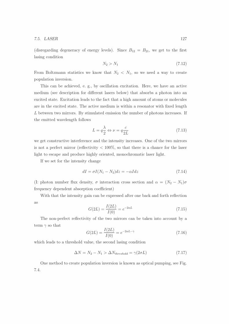
7.5. LASER 127
(disregarding degeneracy of energy levels). Since B12 = B21, we get to the first
lasing condition
N2 > N1 (7.12)
From Boltzmann statistics we know that N2 < N1, so we need a way to create
population inversion.
This can be achieved, e. g., by oscillation excitation. Here, we have an active
medium (see description for different lasers below) that absorbs a photon into an
excited state. Excitation leads to the fact that a high amount of atoms or molecules
are in the excited state. The active medium is within a resonator with fixed length
L between two mirrors. By stimulated emission the number of photons increases. If
the emitted wavelength follows
L = qλ
2⇔ ν = q
c
2L(7.13)
we get constructive interference and the intensity increases. One of the two mirrors
is not a perfect mirror (reflectivity < 100%, so that there is a chance for the laser
light to escape and produce highly oriented, monochromatic laser light.
If we set for the intensity change
dI = σI(N1 −N2)dz = −αIdz (7.14)
(I: photon number flux density, σ interaction cross section and α = (N2 − N1)σ
frequency dependent absorption coefficient)
With that the intensity gain can be expressed after one back and forth reflection
as
G(2L) =I(2L)
I(0)= e−2αL (7.15)
The non-perfect reflectivity of the two mirrors can be taken into account by a
term γ so that
G(2L) =I(2L)
I(0)= e−2αL−γ (7.16)
which leads to a threshold value, the second lasing condition
∆N = N2 −N1 > ∆Nthreshold = γ(2σL) (7.17)
One method to create population inversion is known as optical pumping, see Fig.
7.4.

128 CHAPTER 7. UV-VIS SPECTROSCOPY
Figure 7.4: General scheme for optical pumping.
Excitation goes from the ground state (or any laser level 1) to an excited state
level 3 from which it rapidly falls back on laser level 2 via non-radiative processes.
From laser level 2 the laser emission proceed which competes with a non-radiative
process. The transition rates for the non-radiative processes are denoted as T−132 and
T−121 .
With the pumping rate P = σ13Ip and N3 ≈ PT32N1 ≪ N1, N2, we can define
for the changes in population
dN2
dt= −σ12IL(N2 −N1) −
N2
T21+ PN1 (7.18)
dN1
dt= +σ12IL(N2 −N1) +
N2
T21− PN1 (7.19)
With the definitions ∆N = N2 −N1 and N = N1 +N2 we obtain
d∆N
dt= −2σ12IL∆N0
(
P +1
T21
)
∆N +(
P − 1
T21
)
N (7.20)
In a stationary condition (d∆Ndt
= 0), we get
∆Nstationary =
(
P − 1T21
)
N(
P + 1T21
)
+ 2σ12IL(7.21)

7.5. LASER 129
For the requirement of positive ∆Nstationary, we get
Pcritical =1
T21
(7.22)
This requires that the non-radiative process from level 2 to 1 has to be slow.
7.5.2 Types of Lasers
Lasers are subdivided accordning to the materials that are used. Here, a few exam-
ples will be given.
• Nd-YAG solid-state laser Yttrium aluminum garnet doped with about 1% ne-
doymium is used where the Nd3+ ground state is 4I 92. Due to the YAG crystal
field transitions from the excited states 4F 32
and 4F 52. Pumping wavelengths
is 808 nm and laser emission is 1064 nm which can be changed to 532 nm by
frequency doubling. This is an example of the four-state laser, see Fig. 7.5 to
illustrate the energy levels.
Figure 7.5: Energy diagram for the Nd:YAG laser.

130 CHAPTER 7. UV-VIS SPECTROSCOPY
• Ruby laser The ruby laser represents the first realized laser, created 1960 by
Theodore Maiman. Ruby is corundum, Al2O3 doped with 0.1 % Cr3+. It is
a three-level laser with the ground state being 4A2, the pumping levels 4F2 or4F1 and the upper laser level being a 2E state. This means, that change from
a quartet to a doublet state and vice versa has to occur. The laser wavelength
is 694 nm.
• HeNe laser Helium and neon are mixed in a ratio of 5 to 1. Excitation is done
on the helium atom which transfers energy to neon atoms through collisions.
Three laser transitions with wavelengths of 3.39 µm, 1.15 µm and 633 nm are
generated. The more complicated energy diagram is shown in Fig. 7.6.
Figure 7.6: Energy diagram for the HeNe laser.
• Argon laser Excitation is realized through electron collisions from the atom to
an ionic ground state to the pumping level. About 20 transitions in the range
450 to 530 nm occur due to L and J splittings.

7.5. LASER 131
• CO2 laser Additional to CO2 N2 and He (among others) are present in the gas
chamber to prevent chemical reactions. By electric excitation a metastable N2
level is generated and molecular collisions transfer the energy to CO2. Two
laser levels with 9.6 and 10.6 µm wavelength in the IR correspond to the
symmetric valence vibration and a bending vibration. The energy diagram is
shown in Fig. 7.7.
Figure 7.7: Energy diagram for the CO2 laser.
• semiconductor laser p- and n-doped semiconductors are electrically driven to
achieve polarization inversion and an electron-hole combination happens. For
different semiconductors wavelengths in the range 400 nm to 4µm are possible.
The GaAs laser for instance leads to 850 nm light. Instead of mirrors, often
the crystal boundaries are sufficient.
• dye laser Here dye molecules are dissolved in a solvent such as ethanol, methanol
or water which are often used in flow mode to prevent bleaching of the dye
molecules. The fluorescence from an excited state S1 to the ground state S0
is used. Due to rotation-vibrations broader wavelength ranges are obtained,
typically of 50 nm. Dye lasers are often pumped by other lasers. A lower
efficiency is usually observed compared to other lasers but the high number
of dye molecules easily enables the generation of lasers with strongly different
wavelengths.

132 CHAPTER 7. UV-VIS SPECTROSCOPY
Nowadays, there are also tunable lasers, like the Ti-Sapphire laser existing, that
will not be covered here.
7.6 References
general:
P. W. Atkins, Physical Chemistry, Oxford University Press, Oxford Melbourne
Tokyo, 1990.
W. Demtroder, Experimentalphysik 3, 2nd edition, Springer, 2000.
M. Hesse, H. Meier, B. Zeeh, Spektroskopische Methoden in der organischen
Chemie, Georg Thieme.


![SESI 3 : KERTAS 2 MQF IN PROGRAMMES - Sitik's Blog · SESI 3 : KERTAS 2 MQF IN PROGRAMMES ... (2 long semesters 1 year) [F ÷2] 3.8 3.3 ... 5 English 42 (2+1) 63 14 7 127 3 6 Moral/Islamic](https://static.documents.pub/doc/80x56/5b3f5e6a7f8b9a5e528c0cd5/sesi-3-kertas-2-mqf-in-programmes-sitiks-blog-sesi-3-kertas-2-mqf-in.jpg)

