6 Scaling of two logistic equations, dy/dt = ry(a− y) to dimensionless form. . . . . . . . 13
7 Graph of dy/dt against y for the logistic curve given by dy/dt = ry(a− y). . . . . . . . 14
8 Plots of dy/dt against y for modified logistic equations . . . . . . . . . . . . . . . . . . 15
9 Phase plane diagram for the predator-prey system: dxdt = x(1 − y) (prey) & dy
dt =−y(1 − x) (predator), showing the states passed through between times t1 (state A)and time t2 (state B). . . . . . . . . . . . . . . . . . . . . . . . . . . . . . . . . . . . . 16
10 Graph of yi against i for the chaotic difference equation yi+1 = 4yi(1− yi). . . . . . . . 17
11 Left: The behaviour of the deterministic Lotka-Volterra predator-prey system. Right:The same model with stochastic birth and death events. The deterministic modelpredicts well defined cycles, but these are not stable to even tiny amounts of noise.The stochastic model predicts extinction of at least one type for large populations. Ifregular cycles are observed in reality, this means that some mechanism is missing fromthe model, even though the predictions may very well match reality. . . . . . . . . . . 19
12 Comparison of two models via precision of parameter estimates. . . . . . . . . . . . . . 21
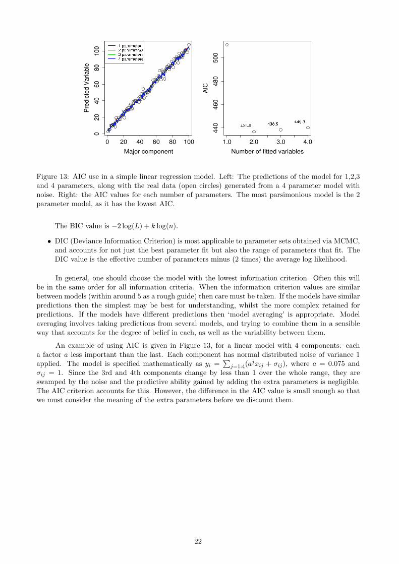
13 AIC use in a simple linear regression model. Left: The predictions of the model for 1,2,3and 4 parameters, along with the real data (open circles) generated from a 4 parametermodel with noise. Right: the AIC values for each number of parameters. The mostparsimonious model is the 2 parameter model, as it has the lowest AIC. . . . . . . . . 22
14 Distribution functions F (x) = Probability(outcome¡x) comparing two scenarios A and B. 25
ii
1 Introduction
1.1 What is mathematical modelling?
Models describe our beliefs about how the world functions. In mathematical modelling, we translatethose beliefs into the language of mathematics. This has many advantages
1. Mathematics is a very precise language. This helps us to formulate ideas and identify underlyingassumptions.
2. Mathematics is a concise language, with well-defined rules for manipulations.
3. All the results that mathematicians have proved over hundreds of years are at our disposal.
4. Computers can be used to perform numerical calculations.
There is a large element of compromise in mathematical modelling. The majority of interactingsystems in the real world are far too complicated to model in their entirety. Hence the first levelof compromise is to identify the most important parts of the system. These will be included in themodel, the rest will be excluded. The second level of compromise concerns the amount of mathematicalmanipulation which is worthwhile. Although mathematics has the potential to prove general results,these results depend critically on the form of equations used. Small changes in the structure ofequations may require enormous changes in the mathematical methods. Using computers to handlethe model equations may never lead to elegant results, but it is much more robust against alterations.
1.2 What objectives can modelling achieve?
Mathematical modelling can be used for a number of different reasons. How well any particularobjective is achieved depends on both the state of knowledge about a system and how well themodelling is done. Examples of the range of objectives are:
1. Developing scientific understanding
- through quantitative expression of current knowledge of a system (as well as displayingwhat we know, this may also show up what we do not know);
2. test the effect of changes in a system;
3. aid decision making, including
(i) tactical decisions by managers;
(ii) strategic decisions by planners.
1.3 Classifications of models
When studying models, it is helpful to identify broad categories of models. Classification of individualmodels into these categories tells us immediately some of the essentials of their structure.
One division between models is based on the type of outcome they predict. Deterministic modelsignore random variation, and so always predict the same outcome from a given starting point. Onthe other hand, the model may be more statistical in nature and so may predict the distribution ofpossible outcomes. Such models are said to be stochastic.
1
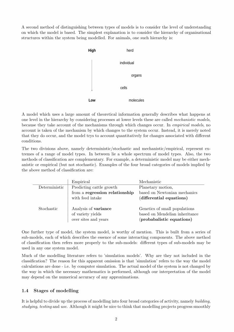
A second method of distinguishing between types of models is to consider the level of understandingon which the model is based. The simplest explanation is to consider the hierarchy of organisationalstructures within the system being modelled. For animals, one such hierarchy is:
Low
herd
individual
High
organs
cells
molecules
A model which uses a large amount of theoretical information generally describes what happens atone level in the hierarchy by considering processes at lower levels these are called mechanistic models,because they take account of the mechanisms through which changes occur. In empirical models, noaccount is taken of the mechanism by which changes to the system occur. Instead, it is merely notedthat they do occur, and the model trys to account quantitatively for changes associated with differentconditions.
The two divisions above, namely deterministic/stochastic and mechanistic/empirical, represent ex-tremes of a range of model types. In between lie a whole spectrum of model types. Also, the twomethods of classification are complementary. For example, a deterministic model may be either mech-anistic or empirical (but not stochastic). Examples of the four broad categories of models implied bythe above method of classification are:
from a regression relationship based on Newtonian mechanicswith feed intake (differential equations)
Stochastic Analysis of variance Genetics of small populationsof variety yields based on Mendelian inheritanceover sites and years (probabalistic equations)
One further type of model, the system model, is worthy of mention. This is built from a series ofsub-models, each of which describes the essence of some interacting components. The above methodof classification then refers more properly to the sub-models: different types of sub-models may beused in any one system model.
Much of the modelling literature refers to ’simulation models’. Why are they not included in theclassification? The reason for this apparent omission is that ’simulation’ refers to the way the modelcalculations are done - i.e. by computer simulation. The actual model of the system is not changed bythe way in which the necessary mathematics is performed, although our interpretation of the modelmay depend on the numerical accuracy of any approximations.
1.4 Stages of modelling
It is helpful to divide up the process of modelling into four broad categories of activity, namely building,studying, testing and use. Although it might be nice to think that modelling projects progress smoothly
2
from building through to use, this is hardly ever the case. In general, defects found at the studyingand testing stages are corrected by returning to the building stage. Note that if any changes are madeto the model, then the studying and testing stages must be repeated.
A pictorial representation of potential routes through the stages of modelling is:
Studying
Testing
Use
Building
This process of repeated iteration is typical of modelling projects, and is one of the most useful aspectsof modelling in terms of improving our understanding about how the system works.
We shall use this division of modelling activities to provide a structure for the rest of this course.
3
2 Building models
2.1 Getting started
Before embarking on a modelling project, we need to be clear about our objectives. These determinethe future direction of the project in two ways.
Firstly, the level of detail included in the model depends on the purpose for which the model will beused. For example, in modelling animal growth to act as an aid for agricultural advisers, an empiricalmodel containing terms for the most important determinants of growth may be quite adequate. Themodel can be regarded as a summary of current understanding. Such a model is clearly of very limiteduse as a research tool for designing experiments to investigate the process of ruminant nutrition.
Secondly, we must make a division between the system to be modelled and its environment. Thisdivision is well made if the environment affects the behaviour of the system, but the system does notaffect the environment. For example, in modelling the growth of a small conifer plantation to predicttimber yields, it is advisable to treat weather as part of the environment. Its effect on growth canbe incorporated by using summary statistics of climate at similar locations in recent years. However,any model for the growth of the world’s forests would almost certainly have to contain terms for theeffect of growth on the weather. Tree cover is known to have a substantial effect on the weather viacarbon dioxide levels in the atmosphere.
2.2 Systems analysis
2.2.1 Making assumptions
Having determined the system to be modelled, we need to construct the basic framework of the model.This reflects our beliefs about how the system operates. These beliefs can be stated in the form ofunderlying assumptions. Future analysis of the system treats these assumptions as being true, butthe results of such an analysis are only as valid as the assumptions.
Thus Newton assumed that mass is a universal constant, whereas Einstein considered mass as beingvariable. This is one of the fundamental differences between classical mechanics and relatively theory.Application of the results of classical mechanics to objects traveling close to the speed of light leadsto inconsistencies between theory and observation.
If the assumptions are sufficiently precise, they may lead directly to the mathematical equationsgoverning the system.
In population studies, a common assumption is that, in the absence of limiting factors, a populationwill grow at a rate which is proportional to its size. A deterministic model which describes such apopulation in continuous time is the differential equation.
dp
dt= ap
where p(t) is population size at time t, and a is a constant. Solution of this equation by integrationgives
p(t) = p(0)eat
where p(0) is population size at time zero. According to this solution, populations grow in size at anexponential rate.
Clearly, not all populations grow exponentially fast. Since the differential equation arose from aninterpretation of the assumption, we must look to the assumption for an explanation for this dis-crepancy. In this case, the explanation is the qualifier ”in the absence of limiting factors”. Most
4
natural populations are subject to constraints such as food supply or habitat which restrict the rangeof sustainable population sizes.
It is important that all assumptions are stated clearly and concisely. This allows us to return to themlater to assess their appropriateness.
Another assumption which we made to obtain the differential equation was that growth takes placecontinuously. If the population consisted of discrete generations, we would have used the differenceequation
di+1 = bdi ,
where di is the size of the ith generation. This has solution
di = d0bi
where d0 is the initial population. Note that the solutions of the differential and difference equationscan coincide at time t = i if d0 = p(0) and b = ea
Yet another assumption we have made is that the population behaves according to a deterministic law.Typically when populations are large we expect randomness or variation to be limited, although as wewill see in Practical 2.1, this can be misleading. However, when populations are small we intuitivelyexpect stochastic variability to be important. This forces us to consider births separately from deaths.A model for population change between times t and t + δt is:
Event Effect on population, p Probability of EventBirth p(t + δt) = p(t) + 1 cp(t)δtDeath p(t + δt) = p(t)− 1 fp(t)δtNo change p(t + δt) = p(t) 1− cp(t)δt− fp(t)δt
This description of the model shows how to (approximately) simulate the stochastic model: choose asufficiently small time step δt (such that all the probabilities are less than one); and then choose oneof the possible events with the probability shown. This last step is achieved by drawing a randomnumber y uniformly on [0, 1] (many packages have such a random number generator). A birth occursif y < cp(t)δt, a death if y < cp(t)δt+fp(t)δt, otherwise no event occurs. Clearly this can be extendedto any number of event types (see e.g. Renshaw 1991 for more details). This stochastic model has thesame expected value as the differential equation model if (c− f) = a. In general, even this degree ofcorrespondence between deterministic and stochastic models is hard to achieve.
Note: In general the correspondence between deterministic and stochastic population models is rathersimple. The model itself is define by the population size p and the rates, for example birth rate, b(p),and death rate, d(p). In the deterministic case these define the rate of change of the population sizen thus,
dp(t)dt
= b(p)− d(p) ,
In the stochastic case these define (for suitably small δt) the probabilities of birth and death events,namely
Event Effect on population, p Probability of EventBirth p(t + δt) = p(t) + 1 b(p)δtDeath p(t + δt) = p(t)− 1 d(p)δtNo change p(t + δt) = p(t) 1− b(p)δt− d(p)δt
A third choice we have made in formulating our simple population growth model is to assumethe population is uniformly distributed in space, and has no contact with other populations. If we were
5
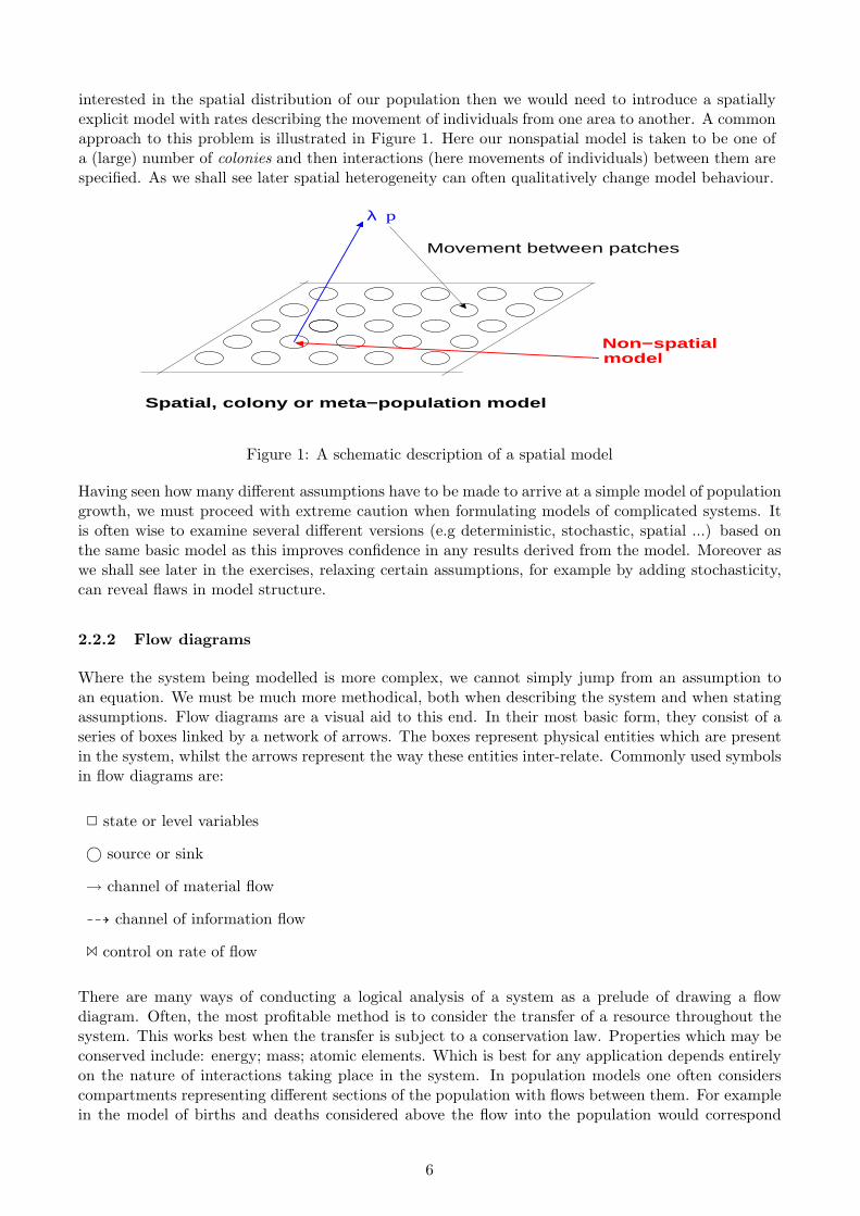
interested in the spatial distribution of our population then we would need to introduce a spatiallyexplicit model with rates describing the movement of individuals from one area to another. A commonapproach to this problem is illustrated in Figure 1. Here our nonspatial model is taken to be one ofa (large) number of colonies and then interactions (here movements of individuals) between them arespecified. As we shall see later spatial heterogeneity can often qualitatively change model behaviour.
λ p
model
Movement between patches
Spatial, colony or meta−population model
Non−spatial
Figure 1: A schematic description of a spatial model
Having seen how many different assumptions have to be made to arrive at a simple model of populationgrowth, we must proceed with extreme caution when formulating models of complicated systems. Itis often wise to examine several different versions (e.g deterministic, stochastic, spatial ...) based onthe same basic model as this improves confidence in any results derived from the model. Moreover aswe shall see later in the exercises, relaxing certain assumptions, for example by adding stochasticity,can reveal flaws in model structure.
2.2.2 Flow diagrams
Where the system being modelled is more complex, we cannot simply jump from an assumption toan equation. We must be much more methodical, both when describing the system and when statingassumptions. Flow diagrams are a visual aid to this end. In their most basic form, they consist of aseries of boxes linked by a network of arrows. The boxes represent physical entities which are presentin the system, whilst the arrows represent the way these entities inter-relate. Commonly used symbolsin flow diagrams are:
There are many ways of conducting a logical analysis of a system as a prelude of drawing a flowdiagram. Often, the most profitable method is to consider the transfer of a resource throughout thesystem. This works best when the transfer is subject to a conservation law. Properties which may beconserved include: energy; mass; atomic elements. Which is best for any application depends entirelyon the nature of interactions taking place in the system. In population models one often considerscompartments representing different sections of the population with flows between them. For examplein the model of births and deaths considered above the flow into the population would correspond
6
INTAKE (I)
(M)
STOREDCHEMICALENERGY (W)
CONVERSIONR3 R5
R4
R2
R1
CONSTRAINTS
R1 + R2 = M
R1 + R3 = I
R3 = R4 + R5
LIVEWEIGHT
MAINTENANCE
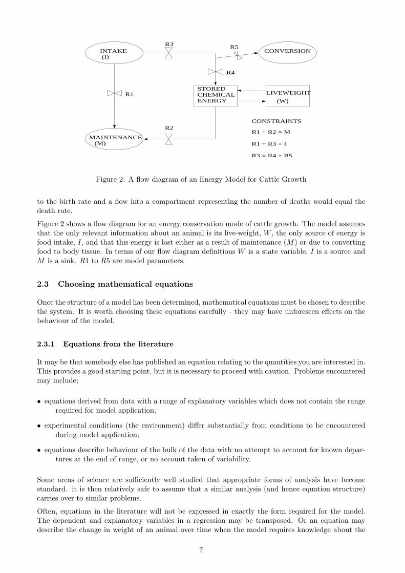
Figure 2: A flow diagram of an Energy Model for Cattle Growth
to the birth rate and a flow into a compartment representing the number of deaths would equal thedeath rate.
Figure 2 shows a flow diagram for an energy conservation mode of cattle growth. The model assumesthat the only relevant information about an animal is its live-weight, W , the only source of energy isfood intake, I, and that this energy is lost either as a result of maintenance (M) or due to convertingfood to body tissue. In terms of our flow diagram definitions W is a state variable, I is a source andM is a sink. R1 to R5 are model parameters.
2.3 Choosing mathematical equations
Once the structure of a model has been determined, mathematical equations must be chosen to describethe system. It is worth choosing these equations carefully - they may have unforeseen effects on thebehaviour of the model.
2.3.1 Equations from the literature
It may be that somebody else has published an equation relating to the quantities you are interested in.This provides a good starting point, but it is necessary to proceed with caution. Problems encounteredmay include;
• equations derived from data with a range of explanatory variables which does not contain the rangerequired for model application;
• experimental conditions (the environment) differ substantially from conditions to be encounteredduring model application;
• equations describe behaviour of the bulk of the data with no attempt to account for known depar-tures at the end of range, or no account taken of variability.
Some areas of science are sufficiently well studied that appropriate forms of analysis have becomestandard. it is then relatively safe to assume that a similar analysis (and hence equation structure)carries over to similar problems.
Often, equations in the literature will not be expressed in exactly the form required for the model.The dependent and explanatory variables in a regression may be transposed. Or an equation maydescribe the change in weight of an animal over time when the model requires knowledge about the
7
t =
10
0
DEN
SITY
(c)
SPACE (x)
Figure 3: Diffusion of a population in which no births or deaths occur.
rate of change. In either case, we may have to accept that the parameter estimates given are notnecessarily the best ones for our purposes.
2.3.2 Analogies from physics
Physicists have built mathematical models to describe a wide range of systems. Often, the systemscan be specified precisely, making the application of mathematical equations relatively simple.
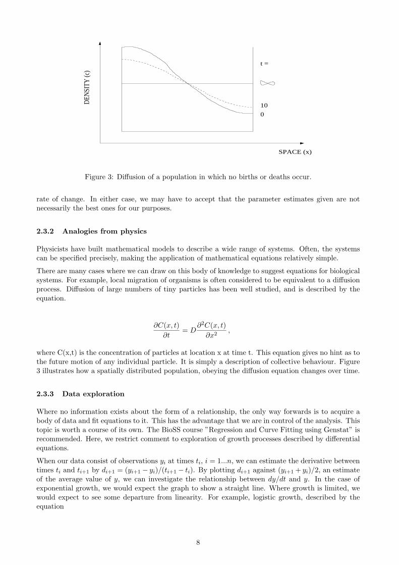
There are many cases where we can draw on this body of knowledge to suggest equations for biologicalsystems. For example, local migration of organisms is often considered to be equivalent to a diffusionprocess. Diffusion of large numbers of tiny particles has been well studied, and is described by theequation.
∂C(x, t)∂t
= D∂2C(x, t)
∂x2,
where C(x,t) is the concentration of particles at location x at time t. This equation gives no hint as tothe future motion of any individual particle. It is simply a description of collective behaviour. Figure3 illustrates how a spatially distributed population, obeying the diffusion equation changes over time.
2.3.3 Data exploration
Where no information exists about the form of a relationship, the only way forwards is to acquire abody of data and fit equations to it. This has the advantage that we are in control of the analysis. Thistopic is worth a course of its own. The BioSS course ”Regression and Curve Fitting using Genstat” isrecommended. Here, we restrict comment to exploration of growth processes described by differentialequations.
When our data consist of observations yi at times ti, i = 1...n, we can estimate the derivative betweentimes ti and ti+1 by di+1 = (yi+1 − yi)/(ti+1 − ti). By plotting di+1 against (yi+1 + yi)/2, an estimateof the average value of y, we can investigate the relationship between dy/dt and y. In the case ofexponential growth, we would expect the graph to show a straight line. Where growth is limited, wewould expect to see some departure from linearity. For example, logistic growth, described by theequation
8
0.0 0.2 0.4 0.6 0.8 1.00.0
0.1
0.2
0.3
0.4
0.0 5.0 10.0 15.0 20.00.0
0.2
0.4
0.6
0.8
1.0
0.0 0.2 0.4 0.6 0.8 1.00.0
0.2
0.4
0.6
0.8
1.0
0.0 5.0 10.0 15.0 20.0−4.0
−3.0
−2.0
−1.0
0.0
y
time time
(y t+1+y t)/2(y t+1+y t)/2
log(y)
(log(y t+1)−log(y t))/δ t
(y t+1−y t)/δ t
Figure 4: The relationship between logistic growth a population data
dy
dt= ry(a− y) ,
should lead to a quadratic curve. Since it is generally rather difficult to determine visually whether ornot a curve is quadratic, we would like to find a plot which gives a straight line when growth followsthe logistic equation. To motivate this plot, we write the logistic equation as
1y
dy
dt= ry(a− y) ,
If we could calculate the left-hand side, sometimes called the proportional growth rate, from the data,then plotting against y would indeed yield a straight line. There is a mathematical result which saysthat
1y
dy
dt=
d
dt(log y) ,
Hence if we calculate (di = log yi+1 − log yi)/(ti+1 − ti) we can proceed as above. This is illustratedin Figure 4. Departure from linearity in the fourth plot not only indicates that the logistic is not thecorrect model for the data, but it may also suggest the kind of amendment, which is appropriate.
2.4 Solving equations
2.4.1 Analytically
There is much to be gained from obtaining an analytical solution to a model. This will allow us toperform all of the manipulations implied by the model with the minimum of fuss. Note that a fullanalytical solution for a stochastic model involves finding the distribution of outcomes, but we mayfeel satisfied if we can solve the equations for the mean and standard deviation. In general, obtainingan analytical solution is rarely a simple matter.
In certain special cases, it is possible to obtain a mathematical solution to a system of equations. Forexample, in compartment analysis we often encounter linked differential equations of the form:
9
dx
dt= ax + by + cz
dy
dt= dx + ey + fz
dz
dt= gx + hy + kz
These equations are linear since there are not product terms of the form xx or xy on the right handside. Because of the properties of linear systems, these differential equations can always be solvedby a standard method. However, the method of solution is restricted to linear systems. If we wereto consider a similar system, which contained just one non-linear term, then we could not apply thismethod. The analytical solution, if it exists, must be sought in other ways.
If the model consists of just one differential equation, then there is a good chance that it has alreadybeen studied. Texts such as Abromowitz and Stegun (1968) contain a large number of standard inte-grals, and it is worth looking to see if the equation of interest is included. Similarly analytic results canalso often be obtained for linear stochastic models. However, when models contain nonlinearity, andmost interesting models do, analytic results are typically harder to obtain than for the correspondingdeterministic system. If the model is more complicated, and especially if the structure of the modelis likely to be changed, then it is hardly worth even trying to find an analytic solution.
2.4.2 Numerically
When analytical methods are unproductive we can use numerical methods to obtain approximatesolutions. Although they can never have the same generality as analytical solutions, they can be justas good in any particular instance.
Numerical solution of model equations generally mimics the processes described in the model. Fordifference equations, numerical solution is exact since we can use the rules laid down in the equationsto follow the evolution of the system. With a stochastic model, we can repeatedly simulate outcomesusing a random number generator as described earlier, and combine a large number of simulations toapproximate the distribution of outcomes.
Differential equations provide a rather more difficult problem. The basic method is to divide continuoustime into discrete intervals, and to estimate the state of the system at the start of each interval. Thusthe approximate solution changes through a series of steps. The crudest method for calculating thesteps is to multiply the step length by the derivative at the start of the interval. This is called Euler’smethod. More sophisticated techniques are used in performing the Runge-Kutte types of integration.Fourth order Runge-Kutte is both commonly used and sufficiently accurate for most applications. It isalways worth treating numerical solutions to differential equations with caution. Errors in calculatingthem may accumulate, as can be seen by considering the following example.
The cosine function y = cos(x), is the solution of the differential equation
d2y
dx2= −y ,
when y(0) = 1 and dy/dx = 0 when x = 0 i.e.,
dy
dx|x=0= 0 ,
This differential equation is equivalent to the linear system
dy
dx= z and
dz
dx= −y
10
0 10 20 30−5
−3
−1
1
3
5
Euler
RK4
Exact
Figure 5: Numerical estimation of the cosine function
when y(0) = 1 and z(0) = 0.
Although the errors inherent in numerical integration of this system using Euler’s method (Figure2.4.2) can be reduced by shortening the step length, this increases the computational burden. Fourthorder Runge-Kutte, on the other hand, can be seen to be much more accurate.
11
3 Studying models
It is important to realise that the behaviour of a model can be described in two ways. Qualitativedescription provides an answer to questions about ”how”, whereas quantitative description answersquestions about ”how much”. In general, qualitative behaviour will be the same for whole families ofmodels and hence is amenable to general results. This contrasts markedly with quantitative behaviour,which is often only relevant to an individual circumstance.
The qualitative behaviour of stochastic models is likely to show more diversity than the correspondingdeterministic models. For example, different realisations of a stochastic population model may exhibitexponential growth and extinction. With stochastic models, therefore, it is important not only todescribe the average behaviour but also to describe the range of types of behaviour.
3.1 Dimensionless form
One way of breaking away from the quantitative features of a particular model is to re-write the equa-tion in terms of dimensionless quantities. This reduces the number of parameters in the equations,making qualitative studies easier and allowing direct comparisons of model types. Having dimension-less quantities also makes direct sense of statements about ”small” or ”large” values.
For example, the differential equation for logistic growth can be written in a dimensionless form whichcontains no parameters. The transformations which lead to this dimensionless form are simply re-scalings of the measurement axes as shown in Figure 3.2. Note that there is an additional parameterin the logistic model corresponding to population size at some specific time. Changing this parametercorresponds to sliding the whole curve, left or right, along the time axis.
3.2 Asymptotic behaviour
A qualitative feature of the (scaled) logistic model is that the long-term behaviour of the population isindependent of the initial conditions. Hence the population will always approach the value 1 as timeincreases. This value is called an asymptote. A population of size 1 is in equilibrium, since accordingto the model it will never change. Furthermore, this equilibrium is stable, since if the population sizeis changed slightly it will always return to 1.
Many other types of long-term behaviour are possible. Some, such as oscillations (also called limitcycles), recur at regular intervals: others continue to display irregular behaviour. Although there areanalytical methods available for studying long-term behaviour of models, we will concentrate only onthe graphical methods.
An alternative way of representing the logistic equation is to plot the derivative dy/dt against y. FromFigure 3.2, we can see that dy/dt is positive for 0 < t < 1 and negative for 1 < y. Hence we candeduce that, in the long run, y will approach a value of 1, although the graph contains no explicitinformation about how fast this will happen.
If the population is not only self-regulating, but is also subjected to a loss of individuals due to someexternal influence, then the logistic model must be amended. One classic example of such a system isfish stocks being depleted by trawlers. If the trawlers operate with constant effort, then it is reasonableto assume that the rate of depletion is cy. As the value of the c increases, the stable population sizedecreases until it reaches zero (Figure 4).
Alternatively, if the trawlers take a catch of constant size, the rate of depletion is simply c. As cincreases, the stable equilibrium value decreases and also the unstable equilibrium value increases. Ifthe population ever falls below the unstable equilibrium, it will carry on decreasing until it becomesextinct. Thus the long-term future of the population depends on the way in which trawling depletesthe population.
12
−10 −5 0 5 10 150.0
1.0
2.0
(i) a=2,r=0.3,y(0)=0.4
(ii) a=0.5,r=0.9,y(0)=0.01y(0)
(a) untransformed
−10 −5 0 5 10 150.0
1.0
2.0
(i)
(ii)
(b) after transformation Y=y/a
−10 −5 0 5 10 150.0
1.0
2.0
(i)
(ii)
(c) after transformation T=ar*t
Standard logistic dY/dT=Y(1−Y)
Figure 6: Scaling of two logistic equations, dy/dt = ry(a− y) to dimensionless form.13
0.0 0.2 0.4 0.6 0.8 1.0 1.2 1.4−0.8
−0.6
−0.4
−0.2
0.0
0.2
0.4
(i)
(ii)
y
dy/dt
Figure 7: Graph of dy/dt against y for the logistic curve given by dy/dt = ry(a− y).
Where two populations are involved, we use a graph called the phase-plane. Figure 9 shows such agraph of the size of one population on the x-axis and the other on the y-axis. Each moment in time isrepresented by one point, and the entire history of the system is represented by a curve. Interactingpopulations can show a wide variety of behaviour. The qualitative features of this behaviour can bestudied without calculating an analytical solution to the equations. Plot the lines for which dy/dt = 0and dx/dt = 0 on the graph. These lines are called the null-clines. Where they cross, the populationshave an equilibrium value. Each equilibrium may be either stable or unstable, depending on thecoefficients in the model.
Not all systems settle down to regular long-term behaviour. Until recently, this was believed to bedue to continual, irregular disturbances from the environment. However, it is now known that evensimple deterministic mathematical models may show apparently erratic behaviour which does not dieaway with time (Figure 10). Such models are called chaotic. Models which exhibit chaotic behaviourare very sensitive to the choice of initial conditions. From two similar initial states, the differencebetween resulting states increases exponentially with time. We will see an example of deterministicchaos in the practical exercises.
We will now move on to consider two quantitative methods for studying models. The first of these,sensitivity analysis, is used to find out how dependent outcomes are on the particular values of chosenparameters. The second method can be used to obtain an approximate understanding of the modelin a few specific cases.
3.3 Sensitivity analysis
The aim of sensitivity analysis is to vary model parameters and assess the associated changes in modeloutcomes. This method is particularly useful for identifying weak points of the model. These can thenbe strengthened by experimentation, or simply noted and caution taken in any application.
If the model is particularly simple, it may be possible to differentiate the outcome with respect to eachparameter in turn. The derivatives give the exact rate of change of predictions with respect to theparameters. With more complicated models, differentiation is best avoided and numerical methodsapplied. Figures 4 and 5
How de we decide on the size of changes to make to each parameter? This choice should depend on
14
0.0 0.2 0.4 0.6 0.8 1.0 1.2 1.4−0.8
−0.6
−0.4
−0.2
0.0
0.2
0.4
(i)
(ii)
y
(a) Constant effort model: dy/dt=y(1−y)−cy
c=0
c=0.3
c=0.6
c=1
0.0 0.2 0.4 0.6 0.8 1.0 1.2 1.4−0.8
−0.6
−0.4
−0.2
0.0
0.2
0.4
(i)
(ii)
y
(b) Constant catch model: dy/dt=y(1−y)−c
c=0
c=0.25
c=0.5
c=0.15
Figure 8: Plots of dy/dt against y for modified logistic equations
15
0.0 0.5 1.0 1.5 2.00.0
0.5
1.0
1.5
2.0
A
Bdx/dt=0
dy/dt=0
x
y
Figure 9: Phase plane diagram for the predator-prey system: dxdt = x(1 − y) (prey) & dy
dt = −y(1 −x) (predator), showing the states passed through between times t1 (state A) and time t2 (state B).
how well the parameter value can be determined. Hence the parameters which have been estimatedfrom data, a multiple of the standard error is appropriate. Some parameters may have to be guessed,in which case a guess at percentage reliability is also required. It is worth remembering that theperson who guessed the parameter value is quite likely to overestimate its reliability. Caution shouldbe taken when parameter estimates are correlated, since if one parameter estimate is changed someof the others might have to be changed too.
3.4 Modelling model output
Evaluating complex models can often take a great deal of computer time. When the model has to beevaluated repeatedly, we may accept some loss of precision in the evaluation if it reduces the time takenper evaluation. Clearly, a reasonable approximation to the model is needed, but when we rememberthat the model itself is only an approximation we will realise that a small loss of detail should be nogreat worry if it speeds up the calculations enough.
There are two ways to proceed. The first is to develop some approximation by simplifying, or sum-marazing the model mathematically. An increrasingly widespread example of this is the use of socalled closure equations to summarize the statistics (typically the mean and variance) of a stochasticmodel. Since closure equations are differential equations the (approximate) results of many stochasticsimulations are obtained for a cost roughly equal to one deterministic model run!
The alternative approach is both simple and more general, but may run against the grain. Firstly,forget all that you know about the interacting equations in the model. Secondly, conduct an experimentin which predictions are obtained from the model for carefully chosen values of the control variables.Thirdly, treat the outcomes as the results of a designed experiment and fit an empirical responsesurface to it. Fourthly, use the fitted surface to estimate model outcomes in the future.
The effectiveness of this procedure depends on a number of issues. Firstly, the model must giveoutcomes which very smoothly with the control variables in the region under consideration, so thatsome simple empirical approximation is possible. Secondly, the supposed experiment must cover thefull range of control variables over which the empirical model will be used. Thirdly, since the problemis that the model outcomes take a long time to calculate, the experiment should be designed to
16
0 20 40 60 80 1000.0
0.2
0.4
0.6
0.8
1.0
1.2
i
yi
Figure 10: Graph of yi against i for the chaotic difference equation yi+1 = 4yi(1− yi).
economise on the number of model evaluations required.
Fortunately, this procedure has been thoroughly covered in the statistical literature. The resultingexperimental designs are called fractional factorial designs. The word fractional refers to the fact thatwe do not have to perform a complete factorial experiment if we are prepared to discard informationabout high-order interactions. The fitted curves which are then used to approximate the model arecalled response curves.
17
4 Testing models
Once we have studied our model and are satisfied with its performance, it is time to begin testing themodel against observations from the physical system which it represents. This process is usually calledvalidation. A similar word, verification, is generally reserved for the non-trivial problem of checkingthat the predictions from the model are faithful to the model description.
What data should we use for testing a model? There is a strong reason for not using the same data aswe used in parameter estimation - it will make us think that the model gives better predictions thanit is really capable of. In linear regression, we correct for the effect of estimating two parameters bydividing the residual sum of squares by (n− 2) instead of (n). In more complicated situations there isno genuine equivalent of the degrees of freedom argument so we have to proceed with greater caution.
In theory, we should test the model assumptions, structure, parameters and predictions. Usually itis necessary to assume a particular functional form; we should check that this isn’t important for thepredictions.
4.1 Testing the assumptions
We should check that we have made the correct assumptions when translating from a verbal modelinto a mathematical model. Assumptions can usually be tested with empirical data as they oftenare models themselves. If there are unwarranted assumptions made in the mathematical model, theyshould be relaxed and the resulting change in model fit checked. Assumptions that can be especiallydangerous include:
• Linearity
• Deterministic dynamics (see Practical)
• ‘Perfect spatial mixing’ (see Practical)
If all is well there will be no qualitative (i.e. behavioural) change in the model predictions whenrelaxing these assumptions, in which case the specific assumption does not matter.
4.2 Model structure
Testing the model structure is usually the most difficult part of testing, particularly in a rigorousway. It often requires a change of methodology, for example, a rewrite of the code, or the needto back analytical work with numerical results. However, unless your model structure is backed byvery strong empirical support, it is important to check that the observed features are not ‘spurious’because you chose a bad model. Figure 11 illustrates a case when the (deterministic) model resultsare spurious because the model is a very special case. Making a small change can break the dynamics,and a stabilising mechanism is needed to truly explain predator-prey cycles. This can be achieved bymaking a small change to the functional form of the model; see Practical 1.
There is no standard way of dealing with model structure problems - it is necessary to simply trymaking changes to assumptions that are not well founded. Model parameters can however be dealtwith in a standard way, but to do so we need some of the concepts introduced in the next section onPrediction.
4.3 Prediction of previously unused data
The most convincing way of testing a model is to use it to predict data which has no connection withthe data used to estimate model parameters. In this way, we reduce to a minimum our chance ofobtaining a spuriously good match between model predictions and data.
18
Figure 11: Left: The behaviour of the deterministic Lotka-Volterra predator-prey system. Right: Thesame model with stochastic birth and death events. The deterministic model predicts well definedcycles, but these are not stable to even tiny amounts of noise. The stochastic model predicts extinctionof at least one type for large populations. If regular cycles are observed in reality, this means thatsome mechanism is missing from the model, even though the predictions may very well match reality.
The phrase ”has no connection with” is an important one. Suppose we were to estimate the parametersof a model by fitting to data collected at a farm over several years. To test the model, we collect moredata from the same farm in the following years. What can this tell us about the model? At best, itwill suggest that the model gives reliable predictions for that one farm. To justify statements aboutthe use of models over a range of farms, the model must be tested over a selection of farms coveringthe entire range.
What summary statistics should we use to describe the discrepancy between data and model predic-tions? For predictions Pi of observations Oi, i = 1...m, we might use:
Bias(B) =1n
Σni=1(Pi −Oi)
Standard deviation (SD) =√
1n
Σni=1(Pi −Oi −B)2
Prediction mean square error (MSE) =1n
Σni=1(Pi −Oi)2 = SD2 + B2
Each of these could be plotted against a chosen variable to test for homogeneity in performance. It isoften a good idea to scale these summary statistics by the mean observation. This makes the summarystatistics independent of units of measurement.
It seems intuitively reasonable that the graph of observations against predictions should show a straightline with unit slope, passing through the origin. Although it is certainly true that a good model wouldbe expected to give rise to a straight line, it is not true that the expected regression has unit slope.The reasons for this apparent paradox are difficult to understand, but nevertheless it is a feature whichis readily observable.
19
4.3.1 Reasons for prediction errors
What are the reasons for imperfect predictions? If we can understand why prediction errors occur,then we have a basis for deciding how to react to them. In general terms, there are three reasons.
Firstly, there is natural variability in the system and its environment. This is what we normally regardas being measurement error in our experiments. We may have a feel for the potential size of theseerrors from previous work. In this case, we will know when to look for other sources of error.
Secondly, there is the effect of factors which we have ignored. Whether such effects can be distinguishedfrom natural variability depends on the amount of additional information recorded as a safeguardagainst this problem. It is advisable to spend time considering how graphical methods can be usedto track down such defects, since actually making changes to the structure of a model can be time-consuming.
Thirdly, some proportion of the errors are attributable to mis-specification of the model. They maybe due to either to errors in functional form, or to parameter estimates. In either case, we can proceedby making the minimum adjustments to the model equations which are necessary to fit well to thetest data. We also have to decide whether such changes are compatible with previous data.
4.4 Estimating model parameters
Estimation of model parameters clearly comes before assessing model performance. However we willdiscuss it here because it is related to the measures of performance (B, SD and MSE) discussed above.If we have a set of data D and wish to determine model parameters from this data one obvious ideais to minimise one of our performance measures with respect to the parameter values. This will givea best fit set of parameters. This also helps to explain why we should use different data for validationand model fitting, since our parameter estimation ensures a good fit to the latter. A common choicefor parameter estimation is to minimise the mean square error. One perceived advantage of this is thatif one assumes that errors in the data are normally distributed and uncorrelated between observationsOi then the slope of the error surface around the minimum parameter values can be used to calculatethe standard errors in the parameter estimates. The problem with this is that the assumption ofnormality may not be valid, and often the data points can not reasonably be considered uncorrelated(e.g. population size - or any other variable!) over time.
In the case of stochastic models a more statistically well founded method of parameter estimationis available since in principle it is possible to construct the likelihood L(D | p) which is simply theprobability that the model with parameters p generated the observed data D . The likelihood is afunction of the model parameters (and the observed data) and may therefore be considered to definethe probability of the parameters given the data. By maximising with respect to the parameterswe can obtain the maximum likelihood estimates of the parameters, and of course we also knowtheir full probability distribution (including standard errors). Moreover, we have made no additionalassumptions beyond those that went into the model. So where’s the catch? Unfortunately it can bedifficult to calculate the likelihood when the data contain missing events (e.g. births and deaths). Insuch cases, and in practice this is all cases, the missing data must be averaged over typically usingcomputationally time consuming methods such as Markov Chain Monte Carlo (MCMC). This is arapidly developing area, but currently most parameters are estimated via minimisation of the meansquared error.
Likelihood methods can be used for deterministic models, although in a theoretically unsatis-factory way. If we assume the the model is correct, then any deviation from that is observation error.In this way the model becomes stochastic by incorporating stochastic observations of a deterministicmodel. This has the advantage that a wide variety of theoretical tools become available; however,since not all the deviation does come from observation error, it may not always work as expected.
20
0 2 4 6 8 100.02
0.04
0.06
0.08
0.10
0.12
0.14
P(b|Data 1)
P(b|Data 2)
Likelihoods for biological control parameter
Figure 12: Comparison of two models via precision of parameter estimates.
4.5 Comparing two models for the same system
When two models of the same system are available, we may want to compare them with an eyeto choosing one for future use. Such a comparison will always contain an element of subjectivity,since there are many different aspects on which the decision can be based. Examples of these aregenerality, predictive ability and computing requirements. To perform a systematic analysis, considerthe building, studying and testing stages in turn.
A good place to begin any comparison is with the underlying assumptions. How do they differ?Presumably there must be some differences, or the models would be identical. If the differences arestructural, it is likely that they are designed to be used in rather different circumstances. Which isclosest to the proposed application? How important are missing interactions known to be?
Once we have tracked down the differences, we are in a position to ask how much effect they arelikely to have on specific applications. Plot out predictions from the models under a range of carefullychosen scenarios. Do they differ sufficiently to cause concern? Two points are worth stressing here.Firstly, small differences are generally not worth worrying about since all models are only approxi-mations. Secondly, beware of models where calculations are repeated iteratively because apparentlysmall differences may accumulate to form substantial differences.
All things being equal, the final choice may be a pragmatic one. Try comparing model predictionswith independent observations. Contrast the models by way of summary statistics of the errors. Atthe same time as comparing the models, this is also a direct test of whether either model is adequatefor the application.
Figure 12 shows an example where model parameters are estimated from data form two treatments.In treatment 1 the biocontrol parameter b is estimated with reasonable precision. However, under thesecond treatment this parameter is poorly estimated (large standard error). This suggests that dataset 2 does not support the biocontrol sub-model and therefore that an alternative model without thiscomponent should be preferred in this case.
There are standard ways of choosing between models, although they usually require some rela-tionship between the models to be simply interpreted. If a model has Likelihood L, uses k parameters,and there are n independent data points available, then the following Information Criterion could beused:
• AIC (Akaike Information Criterion): Defined for nested models (that is, each model is a subse-quent simplification), the AIC value is −2 log(L) + 2k.
• BIC (Bayesian Information Criterion): mostly used for time series data and linear regression.
21
Figure 13: AIC use in a simple linear regression model. Left: The predictions of the model for 1,2,3and 4 parameters, along with the real data (open circles) generated from a 4 parameter model withnoise. Right: the AIC values for each number of parameters. The most parsimonious model is the 2parameter model, as it has the lowest AIC.
The BIC value is −2 log(L) + k log(n).
• DIC (Deviance Information Criterion) is most applicable to parameter sets obtained via MCMC,and accounts for not just the best parameter fit but also the range of parameters that fit. TheDIC value is the effective number of parameters minus (2 times) the average log likelihood.
In general, one should choose the model with the lowest information criterion. Often this willbe in the same order for all information criteria. When the information criterion values are similarbetween models (within around 5 as a rough guide) then care must be taken. If the models have similarpredictions then the simplest may be best for understanding, whilst the more complex retained forpredictions. If the models have different predictions then ‘model averaging’ is appropriate. Modelaveraging involves taking predictions from several models, and trying to combine them in a sensibleway that accounts for the degree of belief in each, as well as the variability between them.
An example of using AIC is given in Figure 13, for a linear model with 4 components: eacha factor a less important than the last. Each component has normal distributed noise of variance 1applied. The model is specified mathematically as yi =
∑j=1:4(a
jxij + σij), where a = 0.075 andσij = 1. Since the 3rd and 4th components change by less than 1 over the whole range, they areswamped by the noise and the predictive ability gained by adding the extra parameters is negligible.The AIC criterion accounts for this. However, the difference in the AIC value is small enough so thatwe must consider the meaning of the extra parameters before we discount them.
22
5 Using models
The method of presentation of a model to its eventual user depends to an extent on how much theuser knows about the model. Since, in general, the use will know rather little about the details of themodel, it is a good idea to present all relevant information in model output. This allows the user, notthe programmer, to make the interpretation. It is almost invariably a good idea to check whether aprediction involves hidden extrapolation. Such extrapolation may be taking place either relative tothe data used to build the model, or relative to the data used to test the model.
5.1 Predictions with estimates of precision
If the only output from a model is the prediction of some quantity, how can the user assess the accuracyof the prediction? Of course, this cannot be done, and the user is left in a take-it or leave-it situation.It would be better if the prediction were accompanied by an estimate of precision, such as a standarderror or a confidence interval. These can be obtained from model studying or model testing.
If we have investigated the effect of errors in parameter estimates when studying the model, we canestimate the precision of a prediction by summarising the distribution of potential outcomes. Thisprovides only a minimum estimate of error, since it takes no account of potentially erroneous forms ofrelationships used.
Alternatively, the estimates of error might be carried through from prediction errors analysed whilsttesting the model. This is the best error to use, as it includes contributions from all possible sources.
A direct application of estimates of prediction errors is the calculation of safety margins in feedrelations. We know from experience that even when animals are fed an identical diet, they will growat slightly different rates. Any model which describes the growth of the group will thus have to containa stochastic element. If the target is for animals to gain weight at 1kg per day, choosing a ration fromwhich the average gain is 1kg per day will mean that, on average, half the animals will not meet thetarget. In order for 95% of animals to meet the target, we need to set the average gain to be 1kg perday plus 1.6 standard deviations (assuming a normal distribution).
5.2 Decision support
We now consider the task of embedding models in a economic framework to assist decision-making.Costs are attached to various inputs to the model, such as animal feed or plant fertiliser. Input levelsare chosen in a way that satisfies any constraints on the system. Conditional on the level of theseinputs, the model is used to estimate biological outputs. The biological outputs themselves will havea financial value (e.g. sale price) attached to them. The difference between output and input valuesis then an estimate of gross profit.
The aim of economic analysis may be to find the strategy which will be the most profitable. Forsimple models with a few control variables, this is usually not too difficult. When there are just twocontrol variables, a graphical treatment is adequate. Numerical methods such as linear or quadraticprogramming may be applicable, but inaccuracies in the model predictions or economic conditionsmay render the extra number of significant figures calculated spurious.
For complex systems with many control variables, optimisation may be a difficult problem. In spe-cial cases, it may be possible to adapt the problem so that linear or quadratic programming areapplicable. Alternatively, a response surface could be fitted, treating profit as the variable to be pre-dicted. Advanced methods such as dynamic programming may be needed to search through the webof interrelated decisions.
Where the model outcome is stochastic, it is rarely possible to make statements like ”strategy A isalways more profitable than strategy B”. Instead, we have to make statements about probabilities,
23
like ”the average profit for strategy A is greater than the average profit for strategy B”. If this istrue, would we always be wise to choose strategy A? The answer of course is no. It might be thatstrategy A has a 40% chance of leading to bankruptcy, but a 60% chance of creating huge profits. Noteverybody would be prepared to take the risks associated with strategy A.
One aid to making decisions between strategies with random outcomes is the concept of stochas-tic dominance. Strategy A is said to dominate strategy B if, for all possible outcomes x, theprobability that the outcome exceeds x is greater for strategy A than for strategy B. To ex-press this condition mathematically, we need to define the distribution function for strategy A asFA(x) = Probability(outcome < x) and, similarly, FB(x). Then strategy A dominates strategy B ifFA(x) < FB(x). This implies that the graph of FA(x) against x lies to the right of the graph FB(x)(Figure 5.2a).
The theory of stochastic dominance has been extended to cover cases where, in the above sense, neitherA dominates B nor B dominates A. For example, second order stochastic dominance is exhibited byA if
∫ r
FB(x)dx >
∫ r
FA(x)dx for all values of r.
This implies that, averaging over all outcomes up to r, FA(x) < F )B(x). Graphically, it means that, tothe left of any value x = r, the area above the curve FB(x) but below FA(x) (Figure 5.2b). Althoughwe would expect everybody to choose strategy A if it dominates strategy B, not everybody wouldchoose strategy A if it only displayed second order dominance. People who choose a strategy basedon second order dominance are said to be ”risk averse” because it indicates the safest bet.
24
−20.0 0.0 20.0 40.00.0
0.2
0.4
0.6
0.8
1.0
FB(x)
FA(x)
(a) Strategy A stochastically dominant over B
x
−20.0 0.0 20.0 40.00.0
0.2
0.4
0.6
0.8
1.0
FB(x)
FA(x)
(b) A shows 2nd−order stochastic dominance over B
x
Figure 14: Distribution functions F (x) = Probability(outcome¡x) comparing two scenarios A and B.
25
6 Discussion
This course has displayed the range of activities involved in mathematical modelling. We shall reinforcethe ideas introduced previously by discussing how to describe a model. Our final comments reach rightback to the outset, when we give some comments about identification of systems which are amenableto modelling and the signals that most of the benefits of a modelling exercise have been achieved.
6.1 Description of a model
There are tow questions to be addressed. The first of these is what information needs to be present.The second is how to go about it.
A good start is a description of the system being modelled. This should put the system into context,reviewing the existing literature and describing the known features which have either been includedin the model or discarded as unimportant. It is no embarrassment to exclude known effects from themodel. The ultimate judgement is likely to be pragmatic: is the model useful.
This leads directly to a statement of the assumptions made. If they are contentious, then somejustification will be necessary. Remember that assumptions are made in sequence. Firstly, thereare the assumptions which relate to breaking an interacting system down into a form which can bemodelled. Secondly, there are assumptions about the interactions between the components of themodel. These may be either qualitative or quantitative.
Quantitative assumptions are usually centred on the choice of equations used, together with parameterestimates and standard errors. It is a good idea to present a table which contains details of the sourceof the equations and their range of application.
The mathematical model itself is the synthesis of these qualitative and quantitative assumptions. Ifthe model calculations are performed algebraically, give details of the calculations in an appendix.If the numerical methods are used, they will need describing carefully including an appraisal of theaccuracy of any approximations. Well-chosen graphs can be a tremendous help.
How was the model studied and tested? It is a good bet that no corrections will have been made todefects unless they have been considered in detail. Given your experiences, what future work will beof most value in improving the model. What levels of precision can you confidently ascribe to thepredictions. If none is given, the reader should assume that either none have been calculated, in whichcase the modeller is flying blind, or there is something to hide.
Finally, it is important to give a clear statement of the range over which the model is believed to bevalid. Remember that this range depends on both the data used to build the model and the data usedto test the model. Scatter-plots are again useful, since these ranges may not be simple to describe.
6.2 Deciding when to model and when to stop
Back in Section 1 we gave some objectives which mathematical modelling may help achieve. But howcan we assess whether a project will be a success, or at what point we should decide that sufficientgain has been made so that we should stop modelling and turn elsewhere? Although the best aid tomaking these decisions is experience, some pointers can still be given.
Modelling is most profitable when the interactions between components of a system have been studied,but the system has not yet been considered as a coherent unit. If a small number of interactions areknown, it may be possible to estimate them from studying the system as a whole. In the end, it isgenerally necessary to sketch out the structure of a model and see how many gaps there are in ourknowledge.
It is time to stop modelling either when the goals of a modelling project have been achieved, or when
26
there is a dearth of information of a sufficient quality. If information about some components simplydoes not exist, it may be worth performing experiments to plug this gap. Only when the gap hasbeen filled is it worth reconsidering the decision not to model. There is always a danger that, once themodel has satisfied one set of criteria, a more stringent set of criteria is introduced on the assumptionthat it is worth trying to do better. If a better model is really needed, try to identify the weakest linkin the model and see how this can be improved. Working away at the remainder of the model will nothelp.
27
Further Reading
For a fuller discussion of material covered on this course, the following books are recommended.Modelling being such a broad subject, each book covers only some aspects.
Bender, E.A. 1978. An introduction to mathematical modelling. Wiley, New York.
An Outline of basic mathematical techniques available to modellers.This is a mathematical text.
Cross, M. and Moscardini, A.O. 1985. Learning the art of mathematical modelling. Ellis HorwoodLtd. Chichester.
A readable, non-technical book on how to start modelling, and how to teach others. It takes adistinctive approach, emphasising that modelling is more art than science.
France, J. and Thornley, J.H.M. 1984. Mathematical models in agriculture. Betterworths, London.
A compendium of published agricultural models, with most emphasis on heavily mathematical,mechanistic ones.
Turchin, P. 2003. Complex Population Dynamics, Princeton University Press, 3 Market Place, Wood-stock, Oxfordshire, OX20 1SY.
An overview of models for ecology, with emphasis on mechasistic models. Covers general theory,types of models, possible behaviour, and fitting to empirical data.
References
Sources mentioned in the text
Abramowitz, M. and Stegun, I.A. 1968. Handbook of Mathematical functions, Dover, New York.Press, W.H., Flannery, B.P., Teukolsky, S.A. and Vetterling, W.T. 1987. Numerical Recipes, Univer-
sity Press, Cambridge, UK.
28
A Modelling energy requirements for cattle growth
Modelling output from the model of energy requirements for cattle growth.
Here we use the energy model to predict animal weight (kg) after 100 days for the 27 combinationsof: starting weight, W0 (150, 20, 250kg): feed intake I (30, 4050 MJ/d); feed quality, q (0.5, 0.6, 0.7).We then fit an empirical regression model to these predictions, using explanatory variables which arelinear or quadratic in W0, I and q.
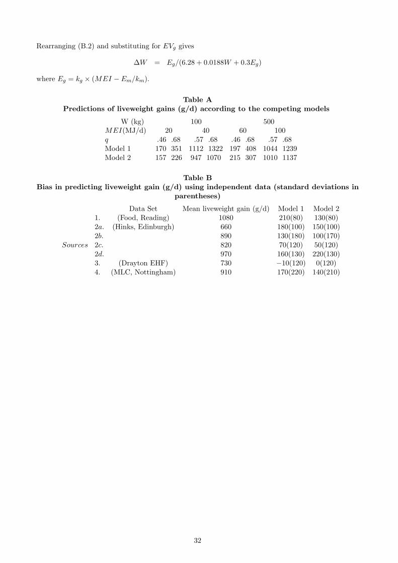
Two models for prediction of liveweight gain in growing cattle
Notation:MEI = metabolisable energy of daily ration (MJ/d)q = ration of metabolisable to gross energy in the dietEm = energy of maintenance (MJ/d)km = efficiency of utilisation of dietary ME for maintenanceL = MEI ∗ km/Em(level of feeding)Eg = energy retained in daily weight change (MJ/d)kg = efficiency of utilisation of dietary ME for weight changeEVg = the energy value of tissue lost or gained (MK/kg)W = liveweight (kg)∆W = liveweight change (kg/d)
General
The daily energy balance in growing cattle may be represented as follows:
Table BBias in predicting liveweight gain (g/d) using independent data (standard deviations in
parentheses)
Data Set Mean liveweight gain (g/d) Model 1 Model 21. (Food, Reading) 1080 210(80) 130(80)2a. (Hinks, Edinburgh) 660 180(100) 150(100)2b. 890 130(180) 100(170)


![FSI - Yoruba Basic Course - Student Text[1]](https://static.documents.pub/doc/80x56/553dd57f55034655428b47fa/fsi-yoruba-basic-course-student-text1.jpg)


