Bioinformatics III “Systems biology” “Integrative cell biology” “Cellular networks” “Computational cell biology”. Course will teach mathematical methods that are applied from protein complexes to interaction networks. Content. Week1networks in biology: effects of different topologies - PowerPoint PPT Presentation
1. Lecture WS 2005/06 Bioinformatics III 1 Bioinformatics III “Systems biology” “Integrative cell biology” “Cellular networks” “Computational cell biology” Course will teach mathematical methods that are applied from protein complexes to interaction networks
Transcript
1. Lecture WS 2005/06
Bioinformatics III 1
Bioinformatics III “Systems biology”
“Integrative cell biology”“Cellular networks”
“Computational cell biology”
Course will teach mathematical methods that are applied
from protein complexes to interaction networks
1. Lecture WS 2005/06
Bioinformatics III 2
Content
Week1 networks in biology: effects of different topologies
Week2 intro of protein complexes: exp. data
Week3 protein networks: computational analysis
Week4 protein networks: graphical layout (force minimization)
Week5 protein networks: quality check (Bayesian analysis)
Week6 protein networks: modularity
Week7 FFT protein-protein docking, fitting into EM maps, tomography
Week8 transcription, regulatory networks, motifs
Week9 integration of interactome and regulome (Lichtenberg)
Week12 mathematical modelling of signal transduction networks
Week13 integration of protein networks with metabolic pathways
Week14 exam
1. Lecture WS 2005/06
Bioinformatics III 3
Appetizer 1
Cell cycle proteins that are part
of complexes or other physical
interactions are shown within
the circle.
For the dynamic proteins, the
time of peak expression is
shown by the node color;
static proteins are represented
as white nodes.
Outside the circle, the dynamic
proteins without interactions
are positioned and colored
according to their peak time.
Lichtenberg et al. Science 307, 724 (2005)
1. Lecture WS 2005/06
Bioinformatics III 4
Appetizer 2
c, Standard statistics (global topological measures and local network motifs) describing network structures. These vary between endogenous and exogenous conditions; those that are high compared with other conditions are shaded. (Note, the graph for the static state displays only sections that are active in at least one condition, but the table provides statistics for the entire network including inactive regions.)
a, Schematics and summary of properties for the endogenous and exogenous sub-networks.
b, Graphs of the static and condition-specific networks. Transcription factors and target genes are shown as nodes in the upper and lower sections of each graph respectively, and regulatory interactions are drawn as edges; they are coloured by the number of conditions in which they are active. Different conditions use distinct sections of the network.
1. Lecture WS 2005/06
Bioinformatics III 5
Appetizer 3
Klamt & Stelling Trends Biotech 21, 64 (2003)
A C P
B
D
A(ext) B(ext) C(ext)R1 R2 R3
R5
R4 R8
R9
R6
R7bR7f
3 EFMs are not systemically independent:EFM1 = EP4 + EP5EFM2 = EP3 + EP5EFM4 = EP2 + EP3
1. Lecture WS 2005/06
Bioinformatics III 6
Mathematical techniques covered
Mathematical graphs – classification of protein-protein interaction networks,
Biological research in the 1900s followed a reductionist approach:
detect unusual phenotype isolate/purify 1 protein/gene, determine its
function
However, it is increasingly clear that discrete biological function can only rarely
be attributed to an individual molecule.
new task of understanding the structure and dynamics of the complex
intercellular web of interactions that contribute to the structure and function of
a living cell.
1. Lecture WS 2005/06
Bioinformatics III 12
Systems biology
Development of high-throughput data-collection techniques,
e.g. microarrays, protein chips, yeast two-hybrid screens
allow to simultaneously interrogate all cell components at any given time.
there exists various types of interaction webs/networks
- protein-protein interaction network
- metabolic network
- signalling network
- transcription/regulatory network ...
These networks are not independent but form „network of networks“.
1. Lecture WS 2005/06
Bioinformatics III 13
DOE initiative: Genomes to Lifea coordinated effort
slides borrowedfrom talk of
Marvin FrazierLife Sciences DivisionU.S. Dept of Energy
1. Lecture WS 2005/06
Bioinformatics III 14
Facility IProduction and Characterization of Proteins
Estimating Microbial Genome Capability
• Computational Analysis– Genome analysis of genes, proteins, and operons– Metabolic pathways analysis from reference data– Protein machines estimate from PM reference data
• Knowledge Captured– Initial annotation of genome– Initial perceptions of pathways and processes– Recognized machines, function, and homology– Novel proteins/machines (including
prioritization)– Production conditions and experience
1. Lecture WS 2005/06
Bioinformatics III 15
• Analysis and Modeling
– Mass spectrometry expression analysis
– Metabolic and regulatory pathway/ network analysis and modeling
• Knowledge Captured– Expression data and conditions– Novel pathways and processes– Functional inferences about novel
proteins/machines– Genome super annotation: regulation, function,
and processes (deep knowledge about cellular subsystems)
Facility II Whole Proteome Analysis
Modeling Proteome Expression, Regulation, and Pathways
1. Lecture WS 2005/06
Bioinformatics III 16
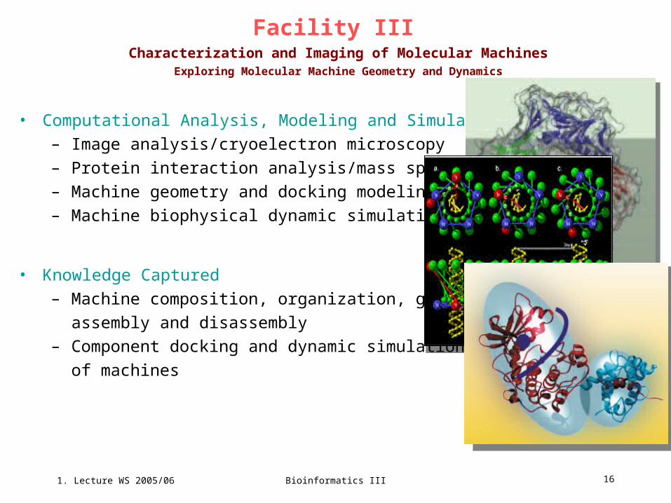
Facility III Characterization and Imaging of Molecular Machines
Exploring Molecular Machine Geometry and Dynamics
• Computational Analysis, Modeling and Simulation
– Image analysis/cryoelectron microscopy
– Protein interaction analysis/mass spec
– Machine geometry and docking modeling
– Machine biophysical dynamic simulation
• Knowledge Captured
– Machine composition, organization, geometry,
assembly and disassembly
– Component docking and dynamic simulations
of machines
1. Lecture WS 2005/06
Bioinformatics III 17
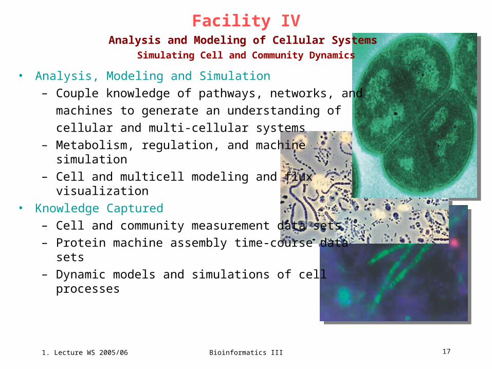
Facility IVAnalysis and Modeling of Cellular Systems
Simulating Cell and Community Dynamics
• Analysis, Modeling and Simulation
– Couple knowledge of pathways, networks, and
machines to generate an understanding of
cellular and multi-cellular systems
– Metabolism, regulation, and machine simulation
– Cell and multicell modeling and flux visualization
• Knowledge Captured
– Cell and community measurement data sets
– Protein machine assembly time-course data sets
– Dynamic models and simulations of cell processes
1. Lecture WS 2005/06
Bioinformatics III 18
“Genomes To Life” Computing Roadmap
Biological Complexity
ComparativeGenomics
Constraint-BasedFlexible Docking
Co
mp
uti
ng
an
d I
nfo
rmat
ion
In
fras
tru
ctu
re C
apab
ilit
ies
Constrained rigid
docking
Genome-scale protein threading
Community metabolic regulatory, signaling simulations
Molecular machine classical simulation
Protein machineInteractions
Cell, pathway, and network
simulation
Molecule-basedcell simulation
Current U.S. Computing
1. Lecture WS 2005/06
Bioinformatics III 19
Are biological networks special?
Albert-Laszlo Barabasi
Statistical physics:
Tries to finding universal scaling laws of systems,
e.g. how does the dynamics of a glass change
when you lower the temperature?
Phase-transition „critical slowing down“.
„Relaxtion times in spin-glasses or glasses are observed to
grow to such an extent at low temperatures that these systems
do not reach thermal equilibrium on experimentally accessible
time-scales. Properties of such systems are then often found to
depend on their history of preparation; such systems are said to
age.
Similar observations are made in coarsening dynamics at first
order phase transitions. Some properties of spin-glasses and
glasses must therefore be studied via dynamical approaches
which allow taking possible history dependence explicitly into
account.“
1. Lecture WS 2005/06
Bioinformatics III 20
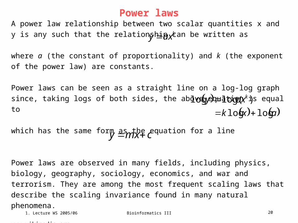
A power law relationship between two scalar quantities x and y is any such that the
relationship can be written as
where a (the constant of proportionality) and k (the exponent of the power law) are
constants.
Power laws can be seen as a straight line on a log-log graph since, taking logs of
both sides, the above equation is equal to
which has the same form as the equation for a line
Power laws are observed in many fields, including physics, biology, geography,
sociology, economics, and war and terrorism. They are among the most frequent
scaling laws that describe the scaling invariance found in many natural phenomena.
www.wikipedia.org
Power laws
kaxy
axk
axy k
loglog
)log(log
cmxy
1. Lecture WS 2005/06
Bioinformatics III 21
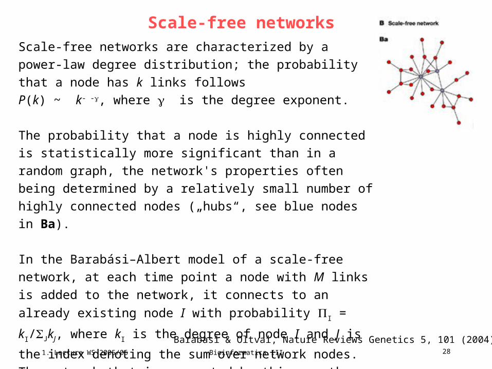
First breakthrough: scale-free metabolic networks
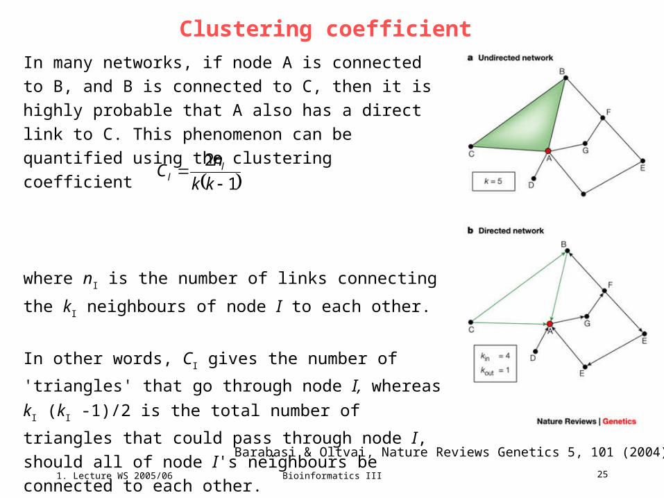
(d) The degree distribution, P(k), of the metabolic network illustrates its scale-free topology.
(e) The scaling of the clustering coefficient C(k) with the degree k illustrates the hierarchical
architecture of metabolism.
(f) The flux distribution in the central metabolism of Escherichia coli follows a power law.