Tesi di Dottorato Universit` a degli Studi di Napoli “Federico II” Dipartimento di Ingegneria Elettrica e delle Tecnologie dell’Informazione Dottorato di Ricerca in Ingegneria Elettronica e delle Telecomunicazioni Covariance Matrix Estimation for Radar Applications Luca Pallotta Il Coordinatore del Corso di Dottorato Il Tutore Ch.mo Prof. Niccol´ o Rinaldi Ch.mo Prof. Antonio De Maio XXVI Ciclo
Transcript
Tesi di Dottorato
Universita degli Studi di Napoli “Federico II”
Dipartimento di Ingegneria Elettricae delle Tecnologie dell’Informazione
Dottorato di Ricerca inIngegneria Elettronica e delle Telecomunicazioni
Covariance Matrix Estimationfor
Radar Applications
Luca Pallotta
Il Coordinatore del Corso di Dottorato Il TutoreCh.mo Prof. Niccolo Rinaldi Ch.mo Prof. Antonio De Maio
XXVI Ciclo
Acknowledgment
I thank Selex ES and SESM for supporting my PhD’s scholarship.Also, I express my gratitude to Dr. Alfonso Farina for his technicalsupport during my research activities, the continuous assistance, en-couragement and kindness demonstrated during these three years.
iii
Contents
List of Figures xi
List of Tables xiv
List of Abbreviations xv
Notations xvii
Introduction 1
1 Structured Covariance Matrix Estimation with a Condi-tion Number Constraint 9
1.5 Spatial processing. Average ORR (expressed in dB) ver-sus nb, where nb = dlog2(Kmax)e is the minimum requiredwordlength. The analyzed environment includes 1 nar-rowband jammer with power σ2
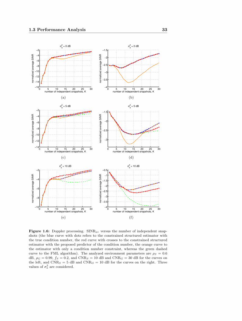
1.6 Doppler processing. SINRav versus the number of inde-pendent snapshots. The analyzed environment parame-ters are ρS = 0.6 dB, ρG = 0.99, fS = 0.2, and CNRS =10 dB and CNRG = 30 dB for the curves on the left, andCNRS = 5 dB and CNRG = 10 dB for the curves on theright. . . . . . . . . . . . . . . . . . . . . . . . . . . . . . . 33
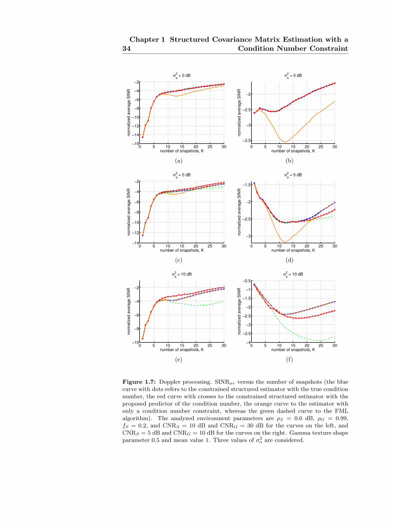
1.7 Doppler processing. SINRav versus the number of snap-shots. The analyzed environment parameters are ρS =0.6 dB, ρG = 0.99, fS = 0.2, and CNRS = 10 dB andCNRG = 30 dB for the curves on the left, and CNRS = 5dB and CNRG = 10 dB for the curves on the right.Gamma texture shape parameter 0.5 and mean value 1. . 34
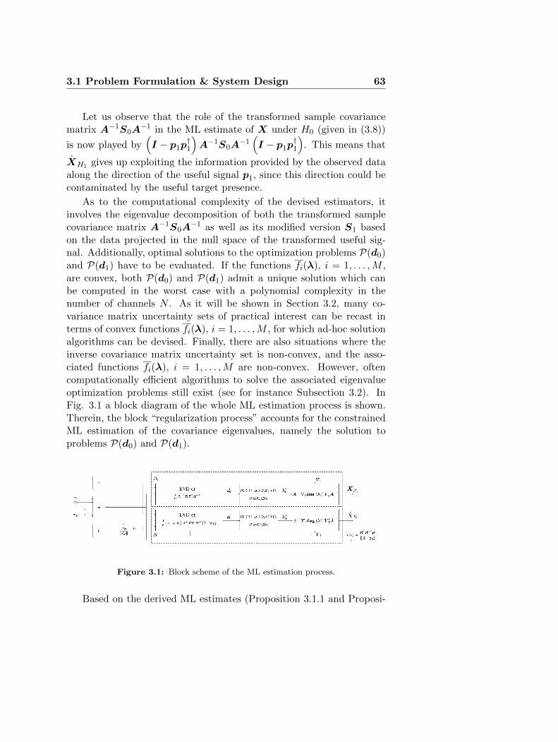
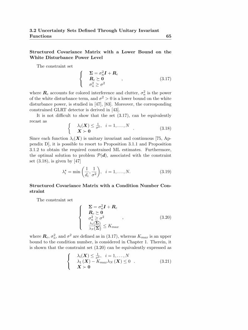
3.1 Block scheme of the ML estimation process. . . . . . . . . 63
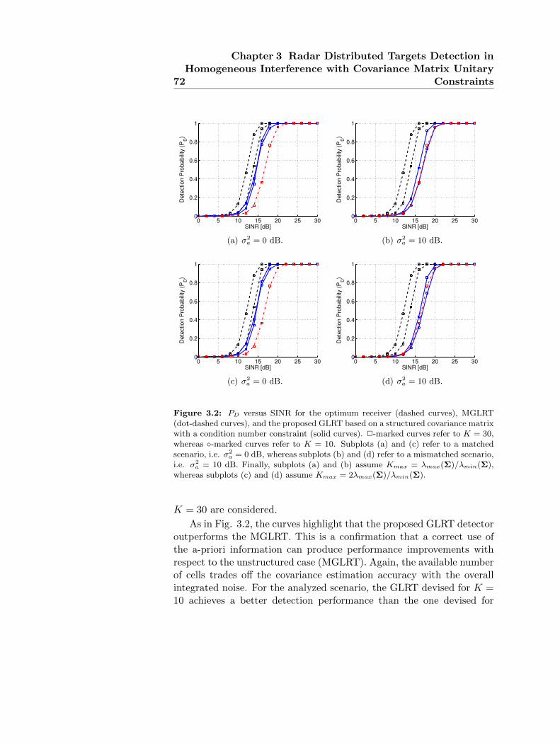
3.2 PD versus SINR for the optimum receiver, MGLRT, andthe proposed GLRT based on a structured covariance ma-trix with a condition number constraint. . . . . . . . . . . 72
List of Figures xi
3.3 PD versus SINR for the optimum receiver, MGLRT, andthe proposed GLRT based on a structured covariance ma-trix with a rank constraint. . . . . . . . . . . . . . . . . . 73
3.4 PD versus SINR for the optimum receiver, MGLRT, andthe proposed GLRT based on a similarity constraint. . . . 75
xii List of Figures
List of Tables
1.1 Maximum SINR gain (in dB) of the proposed estimator,both with the true condition number and its proposedpredictor, with respect to the FML. The values refer tothe simulations of Fig. 1.2. . . . . . . . . . . . . . . . . . 24
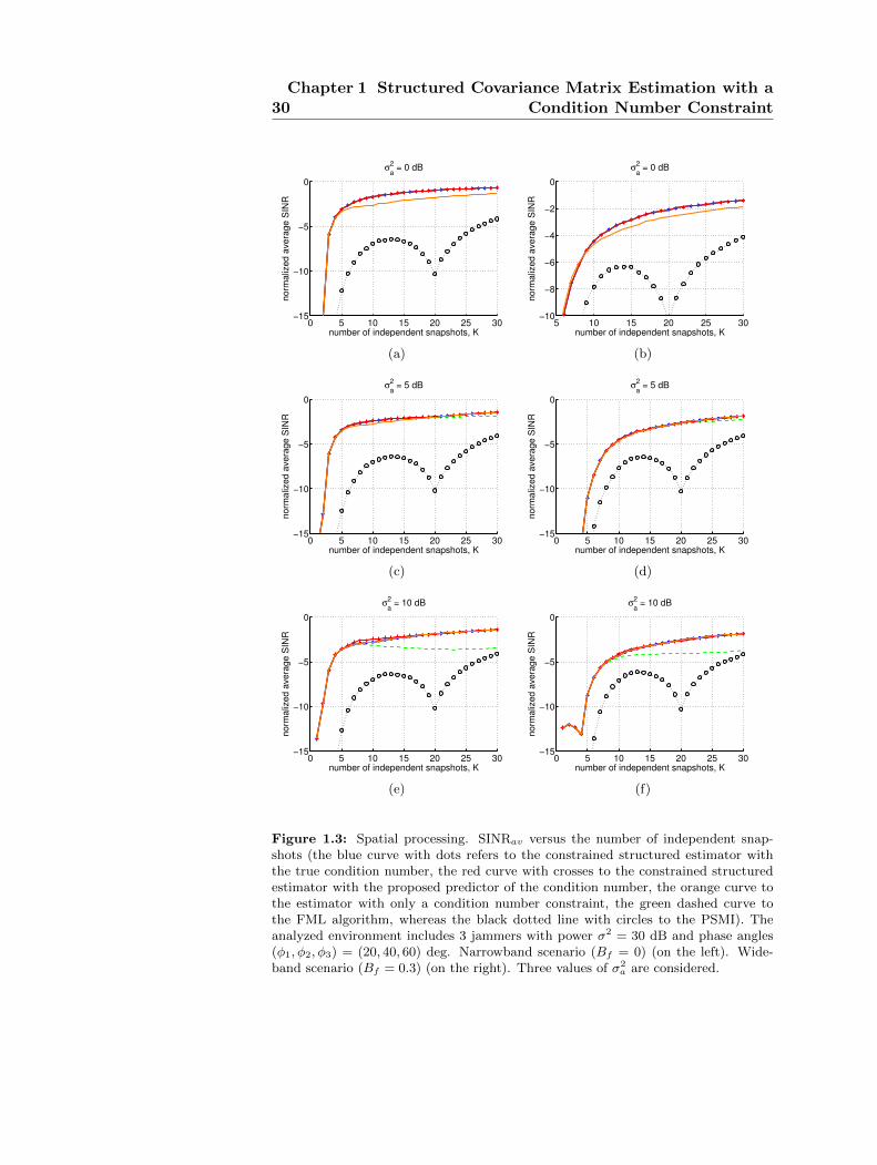
1.2 Maximum SINR gain (in dB) of the proposed estimator,both with the true condition number and its proposedpredictor, with respect to the FML. The values refer tothe simulations of Fig. 1.3. . . . . . . . . . . . . . . . . . 25
1.3 Maximum SINR gain (in dB) of the proposed estimator,both with the true condition number and its proposedpredictor, with respect to the FML. The values refer tothe simulations of Fig. 1.4. . . . . . . . . . . . . . . . . . 25
1.4 Maximum SINR gain (in dB) of the proposed estimator,with the true condition number, with respect to the es-timator with only a condition number constraint. Thevalues refer to the simulations of Fig. 1.2. . . . . . . . . . 25
1.5 Maximum SINR gain (in dB) of the proposed estimator,with the true condition number, with respect to the es-timator with only a condition number constraint. Thevalues refer to the simulations of Fig. 1.3. . . . . . . . . . 25
1.6 Maximum SINR gain (in dB) of the proposed estimator,with the true condition number, with respect to the es-timator with only a condition number constraint. Thevalues refer to the simulations of Fig. 1.4. . . . . . . . . . 25
1.7 Maximum SINR gain (in dB) of the proposed estimator,both with the true condition number and its proposedpredictor, with respect to the FML. The values refer tothe simulations of Fig. 1.6. . . . . . . . . . . . . . . . . . 27
xiii
xiv List of Tables
1.8 Maximum SINR gain (in dB) of the proposed estimator,both with the true condition number and its proposedpredictor, with respect to the FML. The values refer tothe simulations of Fig. 1.7. . . . . . . . . . . . . . . . . . 28
1.9 Maximum SINR gain (in dB) of the proposed estimator,with the true condition number, with respect to the es-timator with only a condition number constraint. Thevalues refer to the simulations of Fig. 1.6. . . . . . . . . . 28
1.10 Maximum SINR gain (in dB) of the proposed estimator,with the true condition number, with respect to the es-timator with only a condition number constraint. Thevalues refer to the simulations of Fig. 1.7. . . . . . . . . . 28
AR AutoregressiveCFAR Constant False Alarm RateCNR Clutter to Noise power RatioCPI Coherent Processing IntervalDOA Direction of Arrivale.m. electromagneticESM Electronic Support MeasuresGIP Generalized Inner ProductGLRT Generalized Likelihood Ratio TestHRR High Resolution Radariid independent and identically distributedLRT Likelihood Ratio TestLMI Linear Matrix Inequalitym.f. matched filterML Maximum LikelihoodMMSE Minimum Mean Square ErrorMGLRT Modified GLRTMTI Moving Target IndicatorNLCD National Land Cover DataORR Output Response Ratiopdf probability density functionPSD Power Spectral DensityPSMI Pseudo Sample Matrix InverseRCS Radar Cross SectionSDP Semidefinite ProgrammingSTAP Space-Time Adaptive ProcessingSINR Signal to Interference plus Noise RatioUMP Uniformly Most Powerfulw.f. whitening filter
xv
Notations
a column vector;A matrix;(·)T transpose operator;(·)† transpose conjugate operator;tr (·) trace of the square matrix argument;det(·) determinant of the square matrix argument;λmin(·) minimum eigenvalue of the square matrix argument;λmax(·) maximum eigenvalue of the square matrix argument;I identity matrix;0 matrix with zero entries;diag(a) diagonal matrix whose i-th diagonal element is
the i-th entry of a;RN set of N -dimensional vectors of real numbers;CN set of N -dimensional vectors of complex numbers;HN N ×N Hermitian matrices;CN,K N ×K matrices of complex numbers;| · | modulus of a complex number;‖ · ‖ Euclidean norm of a complex vector or Frobenius norm
of a complex matrix;λ(A) λ(A) = [λ1(A), λ2(A), . . . , λN (A)], with
λ1(A) ≥ λ2(A) ≥ . . . ≥ λN (A) the vector containingthe eigenvalues of A ∈ HN , arranged in decreasing order;
f(A) for any A = Udiag(λ)U † ∈ HN , withλ = [λ1, λ2, . . . , λN ] the vectors of its eigenvalues, andU the unitary matrix containing the correspondingeigenvectors, it denotes the Hermitian matrix
generalized inequality: A 0 means that Ais an Hermitian positive semi-definite matrix;
generalized inequality: A 0 means that Ais an Hermitian positive definite matrix;
d·e smallest integer greater than or equal to the argument;E [·] statistical expectation;var(·) variance;v(P) optimal value of the optimization problem P;
vec(A) given A ∈ HN , vec(A) = [AT1 ,A
T2 , . . . ,A
TN ]T ∈ CN2
,where Ai is the i-th column of the matrix A.
Introduction
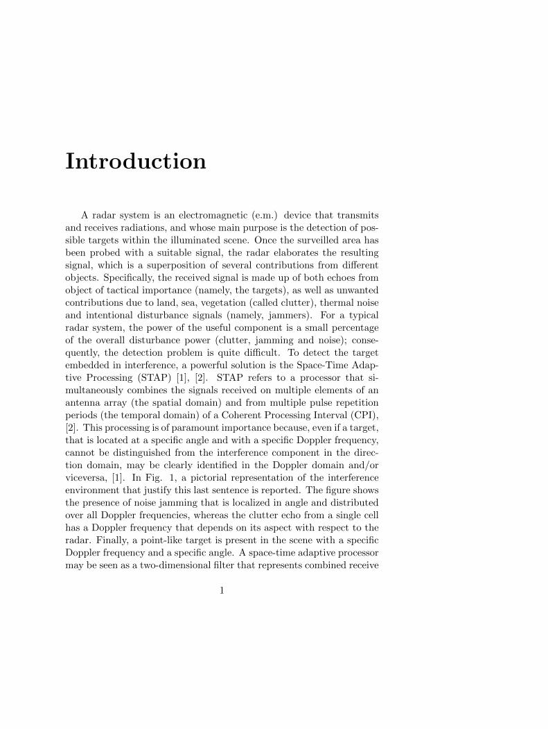
A radar system is an electromagnetic (e.m.) device that transmitsand receives radiations, and whose main purpose is the detection of pos-sible targets within the illuminated scene. Once the surveilled area hasbeen probed with a suitable signal, the radar elaborates the resultingsignal, which is a superposition of several contributions from differentobjects. Specifically, the received signal is made up of both echoes fromobject of tactical importance (namely, the targets), as well as unwantedcontributions due to land, sea, vegetation (called clutter), thermal noiseand intentional disturbance signals (namely, jammers). For a typicalradar system, the power of the useful component is a small percentageof the overall disturbance power (clutter, jamming and noise); conse-quently, the detection problem is quite difficult. To detect the targetembedded in interference, a powerful solution is the Space-Time Adap-tive Processing (STAP) [1], [2]. STAP refers to a processor that si-multaneously combines the signals received on multiple elements of anantenna array (the spatial domain) and from multiple pulse repetitionperiods (the temporal domain) of a Coherent Processing Interval (CPI),[2]. This processing is of paramount importance because, even if a target,that is located at a specific angle and with a specific Doppler frequency,cannot be distinguished from the interference component in the direc-tion domain, may be clearly identified in the Doppler domain and/orviceversa, [1]. In Fig. 1, a pictorial representation of the interferenceenvironment that justify this last sentence is reported. The figure showsthe presence of noise jamming that is localized in angle and distributedover all Doppler frequencies, whereas the clutter echo from a single cellhas a Doppler frequency that depends on its aspect with respect to theradar. Finally, a point-like target is present in the scene with a specificDoppler frequency and a specific angle. A space-time adaptive processormay be seen as a two-dimensional filter that represents combined receive
1
2 Introduction
beamforming and target Doppler filtering [2].
Figure 1: Example of a typical angle-Doppler interference scenario that justifies theuse of a STAP.
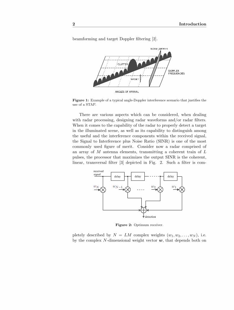
There are various aspects which can be considered, when dealingwith radar processing, designing radar waveforms and/or radar filters.When it comes to the capability of the radar to properly detect a targetin the illuminated scene, as well as its capability to distinguish amongthe useful and the interference components within the received signal,the Signal to Interference plus Noise Ratio (SINR) is one of the mostcommonly used figure of merit. Consider now a radar comprised ofan array of M antenna elements, transmitting a coherent train of Lpulses, the processor that maximizes the output SINR is the coherent,linear, transversal filter [3] depicted in Fig. 2. Such a filter is com-
Figure 2: Optimum receiver.
pletely described by N = LM complex weights (w1, w2, . . . , wN ), i.e.by the complex N -dimensional weight vector w, that depends both on
Introduction 3
the interference statistics as well as on the target signal model. Thus,denoting by
r = p+ n (1)
the N -dimensional vector associated to the received signal of the cellunder test, where p is the steering vector of the useful signal (assumedknown) and n is the zero mean vector associated to the disturbancecomponents, the optimum filter output is given by the inner productbetween the weight vector and the useful signal
s = w†r. (2)
Moreover, denoting by E[nn†] = Σ the disturbance covariance matrix,the SINR at the output of the above mentioned filter is
SINRout =E[|w†p|2]
E[(w†n)(w†n)†]=
∣∣w†p∣∣2w†Σw
=
∣∣∣∣(Σ1/2w)† (
Σ−1/2p)∣∣∣∣2(
Σ1/2w)† (
Σ1/2w)
≤
(Σ1/2w
)† (Σ1/2w
)(Σ−1/2p
)† (Σ−1/2p
)(Σ1/2w
)† (Σ1/2w
)= p†Σp.
(3)
where the inequality in (3) is a consequence of the Schwarz inequality.The latter quantity attains its maximum when the equality holds, i.e.when the two terms in the product at the numerator are proportional,Σ1/2w = Σ−1/2p. Consequently, the optimum receiver is
w = Σ−1p. (4)
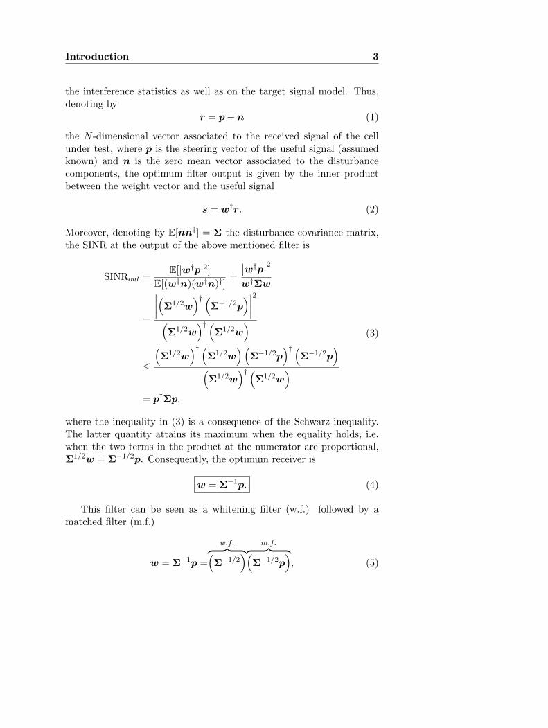
This filter can be seen as a whitening filter (w.f.) followed by amatched filter (m.f.)
w = Σ−1p =
w.f.︷ ︸︸ ︷(Σ−1/2
) m.f.︷ ︸︸ ︷(Σ−1/2p
), (5)
4 Introduction
consequently, the filter is tuned to the Doppler of the target (in a timeprocessing) or to the angle of arrival (in a space processing) or to bothof them in a space-time processing. Moreover, it properly exploits theinformation about the interference statistics (through the disturbancecovariance matrix) in order to reduce the interference effects.
As shown in equation (4), the optimum filter to be applied on thereceived signal requires the exact knowledge of the true disturbance co-variance matrix. However, in real radar systems this requirement cannotbe satisfied and an estimate of the covariance matrix must be introduced,leading to the so-called adaptive radars [4], [5], [6]. Notice also that, ac-curate estimation of the disturbance covariance matrix is of paramountimportance not only for adaptive receive weight vector computation [7],but also for several advanced radar signal processing algorithms, suchas secondary data selection [8] and robust steering vector estimation [9].
Conventional adaptive radar receivers [4], [5], [6], are often based onthe assumption that the environment remains stationary and homoge-neous during the adaptation process. Precisely, they exploit an estimateof the disturbance covariance matrix resorting to a secondary data setcollected from range gates spatially close to the one under test and shar-ing the same spectral properties [10], [11]. A classic estimate is the sam-ple covariance matrix, which is the Maximum Likelihood (ML) estimatorbased on K independent and identically distributed (iid) N -dimensionalzero-mean complex circular Gaussian vectors. The existence of the MLsolution fails when the matrix dimension is greater than the samplesupport (N > K), whereas the sample covariance matrix achieves goodperformance when K ≥ 2N [4]. This homogeneity represents an im-portant limitation since in real environments the number of data inwhich the clutter is homogeneous (often referred to as sample support)is very limited. Poor training data selection, in such adaptive detectors,can result in a remarkable degradation of the adaptive radar perfor-mance especially in regions which include varying ground surfaces suchas coastal regions connecting land and sea, where the strength of theclutter may exhibit strong fluctuations. Some discussions of real-worldeffects and their impacts on the performance of Doppler processors andSTAP detectors can be found respectively in [12] and [13]. A possiblestrategy to circumvent the lack of a sufficient number of homogeneoussecondary data (required for achieving a satisfactory performance) is toexploit some a-priori information about the scene illuminated by the
Introduction 5
radar, namely to perform a knowledge-based processing. Actually thereare two fundamental ways to exploit the available a-priori knowledge([14], [15], and references therein). The former is the indirect approachand uses knowledge sources to select the secondary data for the covari-ance estimation process [14], [15], [16]. The latter is the direct methodand relies on the use of the a-priori knowledge directly in the receiverdesign process [14], [15], [17], [18], [19]. In both cases, it is of interest todevise procedures which exploit jointly the a-priori knowledge availableabout the operating environment and the training data in order to con-fer upon the estimator a robust adaptive behavior. The final goal is toobtain a reliable estimate of the covariance matrix, which must be wellconditioned, since the computation of the weight vector, used in adaptiveradar processing, involves the inverse of the estimated covariance.
As already claimed, in real scenarios the homogeneity assumptionscould not hold, because secondary data may be contaminated by clutterdiscretes, outliers, and/or power variations. Consequently, a statisticalcharacterization of the whole environment can be very difficult to obtain,and estimators, whose design do not rely on the multivariate probabilitydistribution of the data, are of interest. Signal processing algorithms de-rived from geometric considerations on the space of the parameters to beestimated, and which do not account for the statistical characterizationof the data, are available in the open literature. For instance, the leastsquare estimator is the most natural choice [20, Ch. 8, p. 219]. In [21],an extension of the ordered statistic approach, to define a new STAPtechnique, based on the Riemannian p-mean computation of Toeplitz-Block-Toeplitz space-time covariance matrix is presented. Moreover, in[22], an algorithm for radar target detection is introduced, based on theRiemannian p-mean of covariance matrices computed in a neighborhoodof the considered cell. For a detailed overview of this research activ-ity see also [23] and references therein. Finally, the geometric approachis used also in other signal processing contexts; for instance in [24], thebarycenter of a set of diffusion tensors is used in diffusion tensor imagingapplications.
The adaptive receivers previously described refer to point-like tar-gets, namely to targets that are contained within a single range cell.However, it is necessary also to account for radar receivers that operatein presence of targets extended in range. In fact, detection of distributedtargets has gathered extensive attention among radar community during
6 Introduction
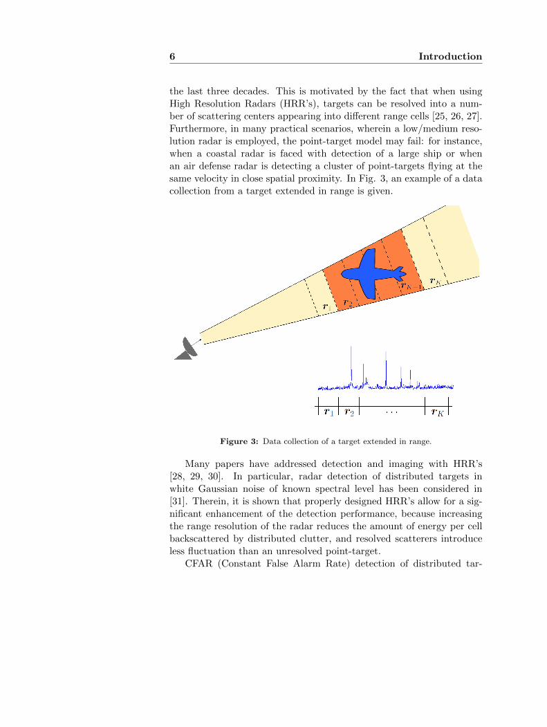
the last three decades. This is motivated by the fact that when usingHigh Resolution Radars (HRR’s), targets can be resolved into a num-ber of scattering centers appearing into different range cells [25, 26, 27].Furthermore, in many practical scenarios, wherein a low/medium reso-lution radar is employed, the point-target model may fail: for instance,when a coastal radar is faced with detection of a large ship or whenan air defense radar is detecting a cluster of point-targets flying at thesame velocity in close spatial proximity. In Fig. 3, an example of a datacollection from a target extended in range is given.
Figure 3: Data collection of a target extended in range.
Many papers have addressed detection and imaging with HRR’s[28, 29, 30]. In particular, radar detection of distributed targets inwhite Gaussian noise of known spectral level has been considered in[31]. Therein, it is shown that properly designed HRR’s allow for a sig-nificant enhancement of the detection performance, because increasingthe range resolution of the radar reduces the amount of energy per cellbackscattered by distributed clutter, and resolved scatterers introduceless fluctuation than an unresolved point-target.
CFAR (Constant False Alarm Rate) detection of distributed tar-
Introduction 7
gets in Gaussian noise with unknown covariance matrix, based uponthe Generalized Likelihood Ratio Test (GLRT) criterion, is addressedin [32, 33, 34, 35, 36, 37] and [38] assuming several (often different)models for the useful target echo. The disturbance returns from dif-ferent range cells are modelled as independent, identically distributed,Gaussian vectors with unknown covariance matrix; moreover, a set ofsecondary data, free of useful signal components, is exploited to estimatethe spectral properties of the disturbance. Some adaptive schemes fordetecting extended targets, assuming the availability of a wide enough,although unknown, portion of secondary data free of the useful signal,are proposed in [39] and [40]. A Modified GLRT (MGLRT) which doesnot resort to secondary data is developed in [41]; it does not share theCFAR property but can be made bounded CFAR, thus being a viabletechnique to adaptively detect range-spread targets embedded in highlynon-stationary environment. The modified GLRT approach is also ap-plied in [42] to develop an adaptive algorithm with orthogonal rejectioncapabilities. A GLRT for the adaptive detection of Doppler-shifted,range-distributed targets embedded in noise with unknown, but struc-tured, covariance matrix has been studied in [43]. Such a detector hasbeen shown to be bounded CFAR via simulation. A heuristic, althougheffective, strategy for detecting range-spread targets in white Gaussiannoise, using multiple consecutive high-resolution range profiles collectedby a HHR, is proposed [44]. A generalized parametric Rao test is devel-oped in [45] modeling the disturbance as a multi-channel auto-regressiveprocess. By doing so the authors extend to distributed targets the in-teresting parametric approach developed in [46] for a point-like target.
All the above considerations highly justify the interest of the researchherein conducted, whose main aim is to define new covariance matrixestimation techniques, based on both statistical argumentations and geo-metric considerations, exploiting advanced mathematics as for instancethe convex optimization theory. These new estimates are utilized todefine new adaptive radar receivers and to design new secondary dataselection schemes, respectively. Moreover, applications to the problemof detecting extended targets have been considered, enforcing severalstructures to the disturbance covariance matrix to estimate.
The present thesis has been organized as follows:
• In Chapter 1, the problem of estimating the disturbance covariancematrix for radar signal processing applications, in the presence of
8 Introduction
a limited number of training data, is addressed. In particular, theML estimator of the covariance matrix is determined starting froma set of secondary data, assuming a special covariance structure(i.e. the sum of a positive semi-definite matrix plus a term pro-portional to the identity), and a condition number upper-boundconstraint. The formulated constrained optimization problem fallswithin the class of MAXDET problems and an efficient procedurefor its solution in closed form is developed. Remarkably, the com-putational complexity of the algorithm is of the same order as theeigenvalue decomposition of the sample covariance matrix.
• In Chapter 2, the problem of covariance matrix estimation forradar signal processing applications is assessed in the presence ofheterogeneous secondary data. In particular, two classes of esti-mators, which do not require any knowledge about the probabilitydistribution of the sample support and exploit the characteristicsof the positive definite matrix space, are proposed and analyzed.Any estimator of each class is associated with a suitable distancein the considered space and is defined respectively as the geomet-ric barycenter and the median matrix of some basic covariancematrix estimates obtained from the available secondary data set.Then, the new devised estimators are applied to the problem ofsecondary data selection.
• In Chapter 3, the problem of detecting an extended target em-bedded in homogeneous Gaussian interference with unknown butstructured covariance matrix is addressed. The possible targetecho, from each range bin under test, is modeled as a determinis-tic signal with an unknown scaling factor accounting for the targetresponse. At the design level, some a-priori knowledge about theoperating environment are exploited, enforcing the inverse inter-ference plus noise covariance matrix to belong to a set describedvia unitary invariant continuous functions. Hence, the constrainedML estimates of the unknown parameters are derived, under boththe H0 and H1 hypotheses, and the GLRT for the considered de-cision problem is designed.
Finally, some conclusions and hints for possible future research tracksare given.
Chapter 1
Structured CovarianceMatrix Estimation with aCondition NumberConstraint
In this chapter, the ML covariance matrix estimator which exploitsthe adaptivity provided by the training data, a special covariance struc-ture, and a condition number upper-bound constraint (whose value canbe obtained from some a-priori information, can be estimated from theavailable samples, or can be set according to numerical stability argu-ments) is devised. Specifically, the covariance matrix is modeled as thesum of two matrices, an unknown positive semi-definite matrix, describ-ing colored interference and clutter, and a (partially known) matrix pro-portional to the identity one, accounting for the white disturbance term.Additionally, the estimated matrix has to comply with an upper boundon its condition number. Notice that, the ML covariance estimationwith the only structural constraint has been considered in [47], whilethe ML estimation of a covariance matrix with only a condition numberupper bound constraint and without any assumptions on its structurehas been studied in [48]. Hence, the novelty of this work is to jointlyaccount for both a structural and a condition number constraint at thedesign level. The core of this work is to show that the proposed con-strained structured ML estimation problem can be formulated in termsof a MAXDET optimization problem [49], [11], and to design a proce-
9
10Chapter 1 Structured Covariance Matrix Estimation with a
Condition Number Constraint
dure for provide its analytically solution in closed form. Notice that,the proposed algorithm requires the computation of the eigenvalue de-composition of the sample covariance matrix and the solution of a scalarconvex optimization problem, whose complexity is linear with respect tothe number of sample eigenvalues greater than one.
At the analysis stage, the performance of the new estimator is as-sessed in terms of achievable SINR versus the number of available sam-ples, both for a spatial and a Doppler processing. The results highlightthat interesting SINR improvements, with respect to the estimators [47]and [48] can be achieved.
Thus, the present chapter is organized as follows. In Section 1.1, thesystem model is described and the main issues arising in a limited samplesupport covariance estimation problem are presented. In Section 1.2, theconstrained structured ML estimation problem is formulated, showingthat it is equivalent to a MAXDET convex optimization problem, andthe procedure for its closed form solution is derived. In Section 1.3, theperformance of the proposed ML estimate is assessed.
1.1 Problem Formulation
In this section, the problem of ML estimating the positive definitecovariance matrix Σ is formulated. Specifically, it is considered theavailability of K secondary data r1, . . . , rK , modeled as N -dimensionalindependent zero-mean complex circular Gaussian vectors1, which sharesthe same covariance matrix
E[rir†i
]= Σ, i = 1, . . . ,K.
To this end, it is necessary to specify the joint probability density func-tion (pdf) of r1, . . . , rK , i.e.
f(r1, . . . , rK |Σ) =1
πNK [det(Σ)]Kexp
[−tr
(KΣ−1S1
)], (1.1)
1The proposed framework assumes Gaussian disturbance. However, there aresituations, such as sea clutter at low grazing angles, where the Gaussian assumptioncan be no longer met and the compound-Gaussian model proves very effective tomodel the radar returns. In this context, alternative covariance matrix estimationstrategies such as those in [50] and [10] can be conceived.
1.1 Problem Formulation 11
where S1 = 1K
∑Ki=1 rir
†i is the sample covariance matrix. Notice that,
owing to the invariance principle [20, Theorem 7.2, p. 176], the MLestimate of Σ (Σ in the following) can be obtained from the ML estimateof X = Σ−1 through a matrix inversion. In particular, without anystructure and constraints on the covariance matrix, i.e. without anya-priori knowledge, the ML estimate of X is an optimal solution to theoptimization problem
X = arg minX0
[tr (S1X) + log det
(X−1
)]. (1.2)
If K ≥ N , (1.2) admits a well known closed form solution X = S−11 ,
namely the inverse of the sample covariance matrix; otherwise, the min-imizer does not exist. This estimate is usually exploited in many adap-tive radar receivers [5, 6, 51, and references therein] and, in particular,for the adaptive implementation of the optimum Doppler, spatial, andSTAP processors [2, 4]. The expected SINR loss, relative to the idealknown covariance case, is kept within 3 dB if the sample support Kis greater than 2N . Unfortunately, in practical radar scenarios, suchan assumption is not always verified [13]. More specifically, the size ofthe training set is often limited, because large swaths of homogeneousclutter/interference necessary for estimating Σ may not be available.Moreover, the presence of the target within the secondary data couldreduce the degree of their homogeneity. In addition, the analysis ofseveral adaptive algorithms, mostly derived assuming homogeneity ofthe secondary data, has shown that non-homogeneities magnify the lossbetween the adaptive implementation and optimum conditions [52, 53].
To reduce the sample support requirement, several solutions havebeen proposed in open literature:
1. to exploit structural information about Σ, as for instance persym-metry [54], Toeplitz property [55], [56], [57], circulant structure[58], multichannel autoregressive models [59], [60], special struc-tures imposed by the sensor and the environment [47], physicalconstraints [61];
2. to resort to Bayesian covariance matrix estimators [62, 63, 64, 65,66];
3. to use knowledge-based covariance models [67, 68];
12Chapter 1 Structured Covariance Matrix Estimation with a
Condition Number Constraint
4. to consider shrinkage estimation methods [69, 70, 19, 48].
The idea followed here is to devise a covariance matrix estimator whichexploits both the adaptivity provided by the training data (even if verylimited) and some a-priori structural information. Namely, a covariancematrix estimator which accounts for a special covariance structure anda condition number upper-bound constraint is designed. Regarding thestructure, the covariance matrix Σ is modeled as the sum of an unknownpositive semidefinite matrix, describing colored interference and cluttercontributes, and a matrix proportional to the identity, accounting forthe white disturbance term. Furthermore, as to the condition numberconstraint, its upper bound value can be obtained (see Subsection 1.2.1)from some a-priori information available at the radar platform aboutthe electromagnetic environment, in an adaptive fashion resorting tothe samples ri, i = 1, . . . ,K, or enforcing a specific value in order tocontrol the numerical stability. In fact, signal processors work with fi-nite precision arithmetic and it is extremely important to account forthe numerical stability of algorithms exploiting the estimated covariancematrix, or its inverse (for instance, adaptive receive weight vector com-putation [7], robust steering vector estimation [9], robust beamforming[71], Direction of Arrival (DOA) estimation, Autoregressive (AR) coef-ficient estimation [72]). Indeed, the effect of the estimated covarianceroundoff error is controlled by the covariance condition number, in thesense that stable algorithms can be obtained if the estimated matrix iswell conditioned with respect to the machine precision [73], [7]. Thus,through the proposed estimator, the idea is to exploit not only the struc-tural information on the covariance matrix, but also to force an upperbound to the condition number compliant with the desired digital sta-bility.
1.2 Derivation of the Constrained StructuredEstimator
Starting from the secondary data r1, . . . , rK , the problem of find-ing the ML estimate of the matrix Σ is considered under the following
1.2 Derivation of the Constrained Structured Estimator 13
constraintsΣ = σ2
nI +R,R 0,σ2n ≥ σ2,λmax(Σ)λmin(Σ)
≤ Kmax,
whereR accounts for colored interference and clutter, whereas σ2n for the
power of the white disturbance term; the parameters σ2 > 0 and Kmax
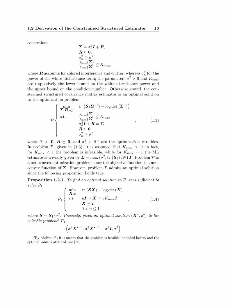
are respectively the lower bound on the white disturbance power andthe upper bound on the condition number. Otherwise stated, the con-strained structured covariance matrix estimator is an optimal solutionto the optimization problem
P
minΣ,R,σ2
n
tr(S1Σ
−1)− log det
(Σ−1
)s.t.
λmax(Σ)λmin(Σ)
≤ Kmax
σ2nI +R = ΣR 0σ2n ≥ σ2
, (1.3)
where Σ 0, R 0, and σ2n ∈ R+ are the optimization variables.
In problem P, given in (1.3), it is assumed that Kmax > 1; in fact,for Kmax < 1 the problem is infeasible, while for Kmax = 1 the MLestimate is trivially given by Σ = max
(σ2, tr (S1) /N
)I. Problem P is
a non-convex optimization problem since the objective function is a non-convex function of Σ. However, problem P admits an optimal solutionsince the following proposition holds true
Proposition 1.2.1. To find an optimal solution to P, it is sufficient tosolve P1
P1
minX ,u
tr (SX)− log det (X)
s.t. uI X uKmaxIX I0 < u ≤ 1
, (1.4)
where S = S1/σ2. Precisely, given an optimal solution (X?, u?) to the
solvable problem2 P1,(σ2X?−1, σ2X?−1 − σ2I, σ2
)2By “Solvable”, it is meant that the problem is feasible, bounded below, and the
optimal value is attained, see [74].
14Chapter 1 Structured Covariance Matrix Estimation with a
Condition Number Constraint
is an optimal solution to P.
Proof. See Appendix A.
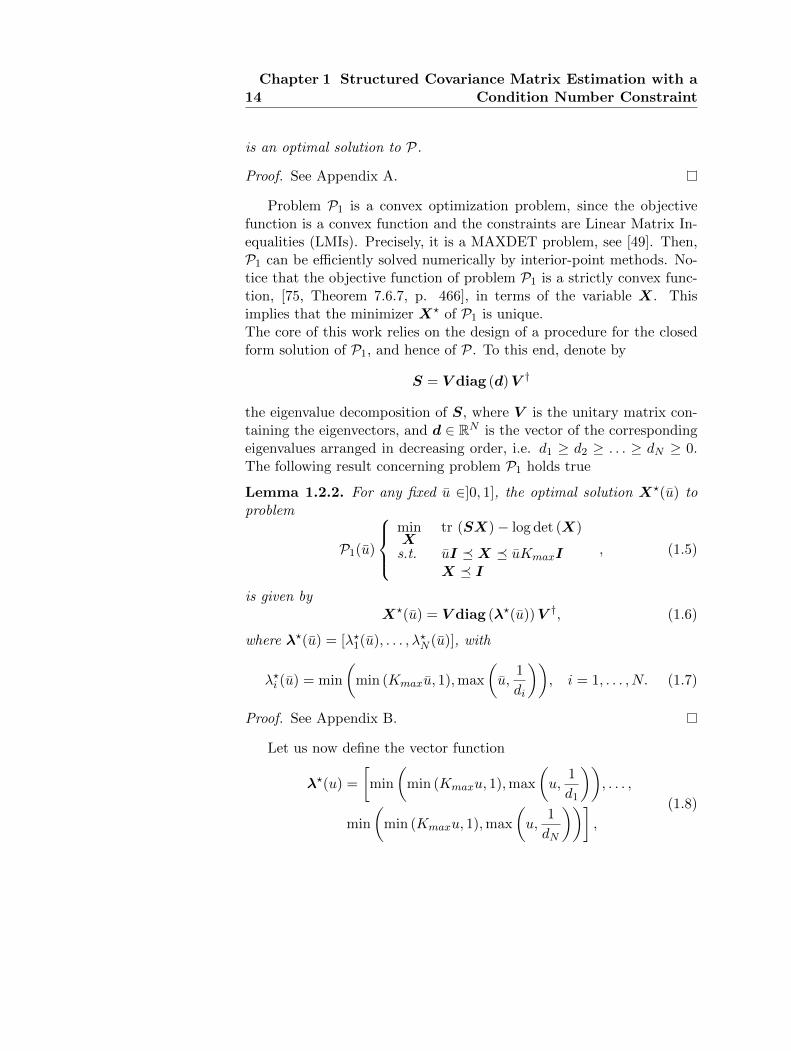
Problem P1 is a convex optimization problem, since the objectivefunction is a convex function and the constraints are Linear Matrix In-equalities (LMIs). Precisely, it is a MAXDET problem, see [49]. Then,P1 can be efficiently solved numerically by interior-point methods. No-tice that the objective function of problem P1 is a strictly convex func-tion, [75, Theorem 7.6.7, p. 466], in terms of the variable X. Thisimplies that the minimizer X? of P1 is unique.The core of this work relies on the design of a procedure for the closedform solution of P1, and hence of P. To this end, denote by
S = V diag (d)V †
the eigenvalue decomposition of S, where V is the unitary matrix con-taining the eigenvectors, and d ∈ RN is the vector of the correspondingeigenvalues arranged in decreasing order, i.e. d1 ≥ d2 ≥ . . . ≥ dN ≥ 0.The following result concerning problem P1 holds true
Lemma 1.2.2. For any fixed u ∈]0, 1], the optimal solution X?(u) toproblem
P1(u)
minX
tr (SX)− log det (X)
s.t. uI X uKmaxIX I
, (1.5)
is given byX?(u) = V diag (λ?(u))V †, (1.6)
where λ?(u) = [λ?1(u), . . . , λ?N (u)], with
λ?i (u) = min
(min (Kmaxu, 1),max
(u,
1
di
)), i = 1, . . . , N. (1.7)
Proof. See Appendix B.
Let us now define the vector function
λ?(u) =
[min
(min (Kmaxu, 1),max
(u,
1
d1
)), . . . ,
min
(min (Kmaxu, 1),max
(u,
1
dN
))],
(1.8)
1.2 Derivation of the Constrained Structured Estimator 15
which assigns to any u ∈]0, 1] the vector of the optimal eigenvalues toproblem P1(u) given in (1.5).
Theorem 1.2.3. Let u? be an optimal solution to the following opti-mization problem
P2
minu
∑Ni=1Gi(u)
s.t. 0 < u ≤ 1, (1.9)
where, for any i = 1, . . . , N , Gi(u) = diλ?i (u)− log λ?i (u), namely
Gi(u) =
− logKmax − log u+Kmaxdiu if 0 < u ≤ 1
Kmaxdi if 1
Kmax≤ u ≤ 1
(1.10)
if di ≤ 1, and
Gi(u) =
− logKmax − log u+Kmaxdiu if 0 < u ≤ 1
Kmaxdilog di + 1 if 1
Kmaxdi≤ u ≤ 1
di− log u+ diu if 1
di≤ u ≤ 1
(1.11)if di > 1. Then, an optimal solution to P1 is
(X?, u?) =(V diag (λ?)V †, u?
), (1.12)
where λ? = [λ?1, . . . , λ?N ] = λ?(u?), with the vector function λ?(u) defined
in (1.8).
Proof. See Appendix C.
Notice that the formulation of Theorem 1.2.3 holds even when di = 0,interpreting 1
di= +∞. Therefore, resorting to Theorem 1.2.3, problem
P1 reduces, essentially, to the univariate minimization problem P2. Letus, now, study the properties of the optimization problem P2, preciselyof its objective function
G(u) =
N∑i=1
Gi(u), (1.13)
with Gi(u) defined in (1.10) or in (1.11), depending on the value of thecorresponding di. Firstly, the function G(u) is a continuous functionover the interval u ∈]0, 1], since it is the sum of continuous functions.Secondly, although the constraint u ∈]0, 1] of problem P2 defines an openset, P2 is solvable as proved in the following theorem
16Chapter 1 Structured Covariance Matrix Estimation with a
Condition Number Constraint
Theorem 1.2.4. Let d1 ≥ d2 ≥ . . . ≥ dN the eigenvalues of S. Theoptimal value v(P2) is attainable and
• if d1 ≤ 1, an optimal solution to P2 is u? = 1Kmax
;
• if 1 < d1 ≤ Kmax, an optimal solution to P2 is u? = 1d1
;
• if d1 > Kmax, an optimal solution to P2 complies with u? ∈[1d1, 1Kmax
].
Proof. See Appendix D.
From theorem 1.2.4, to completely solve P2, it is needed to analyzethe case d1 > Kmax. Hence, it has to be proven
Lemma 1.2.5. Let d1 > Kmax. The function G(u) has a continuous
derivative over the interval u ∈]0, 1
Kmax
]. Moreover, G(u) is a univari-
ate convex function in the interval u ∈]0, 1
Kmax
].
Proof. See Appendix E.
Let us further investigate the characteristics of the univariate convexfunction G(u) when d1 > Kmax; the goal is to exploit its structure inorder to develop an explicit procedure to solve P2. To this end, letus define some auxiliary quantities. Denote by N , the number of di’sgreater than 1, i.e. di > 1, i = 1, . . . , N . The vector v
v = [d1, d2, . . . , dN , 1], (1.14)
contains the eigenvalues greater than 1, and its last entry is equal to1; also, v = [v1, v2, . . . , vN , vN+1] contains its entries in non-increasingorder. Thus, the following theorem is proved
Theorem 1.2.6. Assuming d1 > Kmax, an optimal solution u? to P2
is given by
1) u? = 1d1
, if dG(u)du
∣∣∣u= 1
d1
= 0;
2) u? = 1Kmax
, if dG(u)du
∣∣∣u= 1
Kmax
≤ 0;
1.2 Derivation of the Constrained Structured Estimator 17
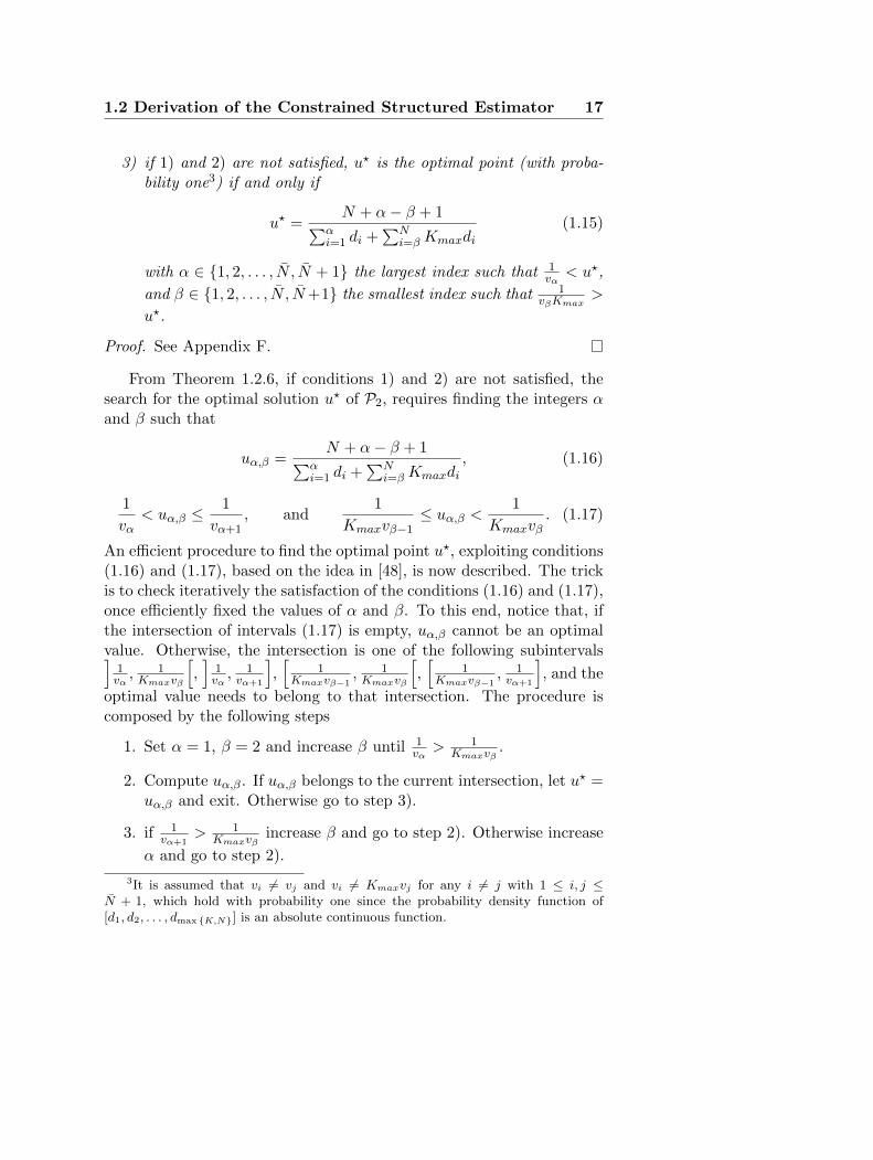
3) if 1) and 2) are not satisfied, u? is the optimal point (with proba-bility one3) if and only if
u? =N + α− β + 1∑α
i=1 di +∑N
i=βKmaxdi(1.15)
with α ∈ 1, 2, . . . , N , N + 1 the largest index such that 1vα< u?,
and β ∈ 1, 2, . . . , N , N+1 the smallest index such that 1vβKmax
>
u?.
Proof. See Appendix F.
From Theorem 1.2.6, if conditions 1) and 2) are not satisfied, thesearch for the optimal solution u? of P2, requires finding the integers αand β such that
uα,β =N + α− β + 1∑α
i=1 di +∑N
i=βKmaxdi, (1.16)
1
vα< uα,β ≤
1
vα+1, and
1
Kmaxvβ−1≤ uα,β <
1
Kmaxvβ. (1.17)
An efficient procedure to find the optimal point u?, exploiting conditions(1.16) and (1.17), based on the idea in [48], is now described. The trickis to check iteratively the satisfaction of the conditions (1.16) and (1.17),once efficiently fixed the values of α and β. To this end, notice that, ifthe intersection of intervals (1.17) is empty, uα,β cannot be an optimalvalue. Otherwise, the intersection is one of the following subintervals]
1vα, 1Kmaxvβ
[,]
1vα, 1vα+1
],[
1Kmaxvβ−1
, 1Kmaxvβ
[,[
1Kmaxvβ−1
, 1vα+1
], and the
optimal value needs to belong to that intersection. The procedure iscomposed by the following steps
1. Set α = 1, β = 2 and increase β until 1vα> 1
Kmaxvβ.
2. Compute uα,β. If uα,β belongs to the current intersection, let u? =uα,β and exit. Otherwise go to step 3).
3. if 1vα+1
> 1Kmaxvβ
increase β and go to step 2). Otherwise increase
α and go to step 2).
3It is assumed that vi 6= vj and vi 6= Kmaxvj for any i 6= j with 1 ≤ i, j ≤N + 1, which hold with probability one since the probability density function of[d1, d2, . . . , dmax K,N] is an absolute continuous function.
18Chapter 1 Structured Covariance Matrix Estimation with a
Condition Number Constraint
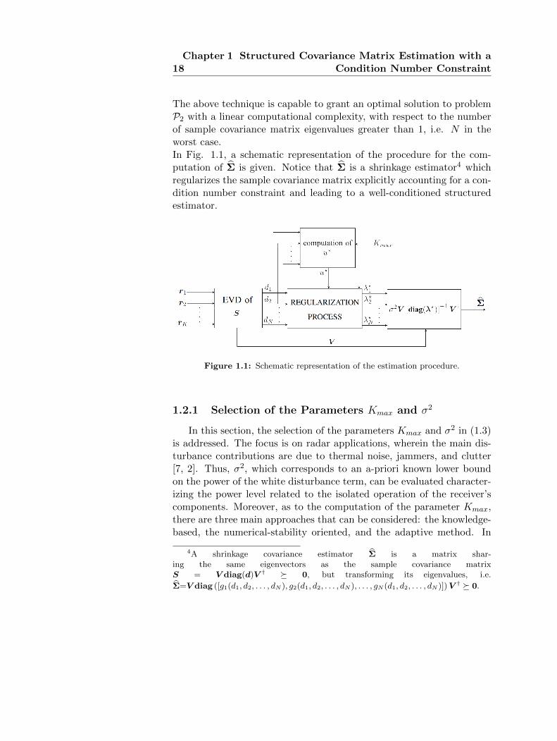
The above technique is capable to grant an optimal solution to problemP2 with a linear computational complexity, with respect to the numberof sample covariance matrix eigenvalues greater than 1, i.e. N in theworst case.In Fig. 1.1, a schematic representation of the procedure for the com-putation of Σ is given. Notice that Σ is a shrinkage estimator4 whichregularizes the sample covariance matrix explicitly accounting for a con-dition number constraint and leading to a well-conditioned structuredestimator.
Figure 1.1: Schematic representation of the estimation procedure.
1.2.1 Selection of the Parameters Kmax and σ2
In this section, the selection of the parameters Kmax and σ2 in (1.3)is addressed. The focus is on radar applications, wherein the main dis-turbance contributions are due to thermal noise, jammers, and clutter[7, 2]. Thus, σ2, which corresponds to an a-priori known lower boundon the power of the white disturbance term, can be evaluated character-izing the power level related to the isolated operation of the receiver’scomponents. Moreover, as to the computation of the parameter Kmax,there are three main approaches that can be considered: the knowledge-based, the numerical-stability oriented, and the adaptive method. In
4A shrinkage covariance estimator Σ is a matrix shar-ing the same eigenvectors as the sample covariance matrixS = V diag(d)V † 0, but transforming its eigenvalues, i.e.
1.2 Derivation of the Constrained Structured Estimator 19
the following subsections, all of them are discussed in detail.
Knowledge-Based Selection of Kmax
A knowledge-based selection of Kmax resorts to a-priori informationavailable at the radar platform about the electromagnetic environment.Precisely, exploiting Electronic Support Measures (ESM), a rough pre-diction of the jammer attributes can be obtained (such as their location,bandwidth, and power). Furthermore, as to the clutter contribution,it can be predicted through the interaction between a digital terrainmap, such as the National Land Cover Data (NLCD), and Radar CrossSection (RCS) clutter models, see [76], [16], [77, Ch. 15, 16]. Startingfrom this information and some a-priori knowledge on the power of thewhite disturbance term, a rough estimate of the condition number of thecovariance matrix can be performed.
Numerical-Stability Oriented Selection of Kmax
An important task, in digital processing design, is the numerical sta-bility of the outputs from the implemented algorithms, with respect tothe accuracy of the input data. Thus, it is extremely relevant to guaran-tee a stable computation with respect to the roundoff errors corruptingthe estimated covariance matrix Σ. It is worth pointing out that thereis a fundamental tradeoff between the number of bits available in thecomputer to accomplish matrix inversion and the allowable eigenvaluespread (ruled by the condition number) of the input covariance [78, pp.312-313], [7, p. 132]. In this context, a suitable choice of Kmax allowsfor a control on the algorithm stability. For instance, the adaptive re-ceive weight vector w is given by the solution of the following linear
system Σσ2w = p, where p is the steering vector. Consequently, due to a
perturbation E of the matrix Σσ2 , [7], the computed weight vector is the
solution to
(Σσ2 +E
)wp = p, where |E (h, k) | ≤ ε′ with ε′ the machine
precision. Thus, from [79], the sensitivity of the weight vector to the
machine precision is upper bounded5 by||w−wp||||w|| ≤ ε′NKmax, i.e. it
can be controlled through an appropriate selection of Kmax.
5A similar result holds true even if p is perturbed.
20Chapter 1 Structured Covariance Matrix Estimation with a
Condition Number Constraint
Adaptive Selection of Kmax
In this subsection, an adaptive estimator of Kmax, based on theK secondary data r1, . . . , rK , is presented. The trainer principle, ex-ploited by the predictor, is to extract information starting from thediagonal blocks of S; each block is the sample covariance matrix of thecorresponding sub-vector extracted by r1
σ , . . . ,rKσ . Indeed, due to the
available sample support K, the estimation of the sub-covariance ma-trix from sub-vectors extracted by r1
σ , . . . ,rKσ might be performed more
reliably than the estimation of the entire covariance matrix. Moreover,given the stationarity property (ensured by the use of either a uniformlinear array or a regularly spaced pulse train) of the random vectorsriσ , i = 1, . . . ,K, the information provided by different diagonal blocks
of S of the same size can be combined to produce an estimate.As to the dimension of the sub-blocks, which are meaningfully to an-
alyze, its value is related to the dimension of the subspace in which thedisturbance concentrates most of its power and depends on the specificradar application. Namely, for a spatial processing, through the analysisof sub-matrices of dimension smaller than or equal to the number J ofjammers, it is difficult to acquire reliable information about the condi-
tion number of the matrix Σσ2 , since all the directions are almost surely
completely affected by the interference power. Consequently, the knowl-edge of J is assumed, whose value can be obtained adaptively resortingto the ESM of the radar platform, and start to analyze sub-blocks of di-mension greater than or equal to J + 1. It is also assumed that J < N ,which is a reasonable assumption in the radar context.
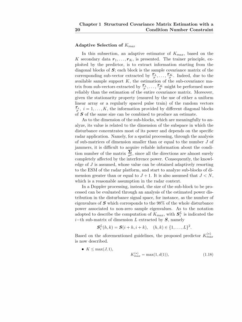
In a Doppler processing, instead, the size of the sub-block to be pro-cessed can be evaluated through an analysis of the estimated power dis-tribution in the disturbance signal space, for instance, as the number ofeigenvalues of S which corresponds to the 98% of the whole disturbancepower associated to non-zero sample eigenvalues. As to the notationadopted to describe the computation of Kmax, with SLi is indicated thei−th sub-matrix of dimension L extracted by S, namely
Based on the aforementioned guidelines, the proposed predictor K(∗)max
is now described.
• K ≤ max(J, 1),K(∗)
max = max(1, d(1)), (1.18)
1.3 Performance Analysis 21
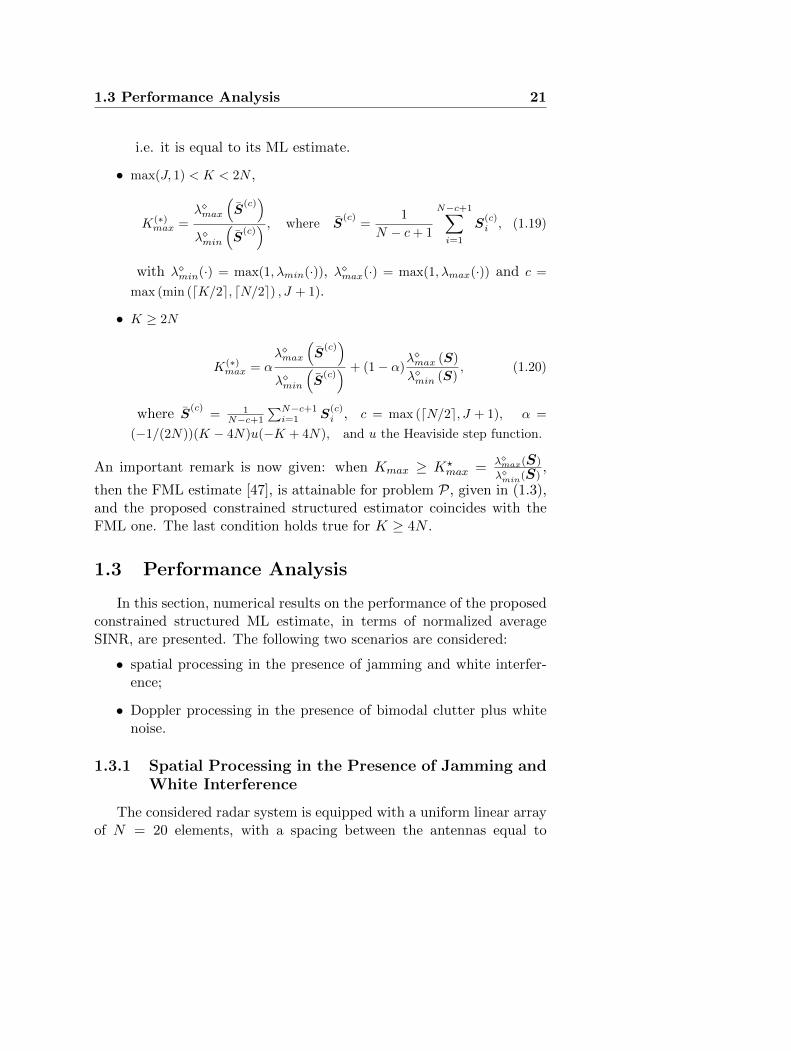
i.e. it is equal to its ML estimate.
• max(J, 1) < K < 2N ,
K(∗)max =
λmax
(S
(c))
λmin
(S
(c)) , where S
(c)=
1
N − c+ 1
N−c+1∑i=1
S(c)i , (1.19)
with λmin(·) = max(1, λmin(·)), λmax(·) = max(1, λmax(·)) and c =
max (min (dK/2e, dN/2e) , J + 1).
• K ≥ 2N
K(∗)max = α
λmax
(S
(c))
λmin
(S
(c)) + (1− α)
λmax (S)
λmin (S), (1.20)
where S(c)
= 1N−c+1
∑N−c+1i=1 S
(c)i , c = max (dN/2e, J + 1), α =
(−1/(2N))(K − 4N)u(−K + 4N), and u the Heaviside step function.
An important remark is now given: when Kmax ≥ K?max = λmax(S)
λmin(S),
then the FML estimate [47], is attainable for problem P, given in (1.3),and the proposed constrained structured estimator coincides with theFML one. The last condition holds true for K ≥ 4N .
1.3 Performance Analysis
In this section, numerical results on the performance of the proposedconstrained structured ML estimate, in terms of normalized averageSINR, are presented. The following two scenarios are considered:
• spatial processing in the presence of jamming and white interfer-ence;
• Doppler processing in the presence of bimodal clutter plus whitenoise.
1.3.1 Spatial Processing in the Presence of Jamming andWhite Interference
The considered radar system is equipped with a uniform linear arrayof N = 20 elements, with a spacing between the antennas equal to
22Chapter 1 Structured Covariance Matrix Estimation with a
Condition Number Constraint
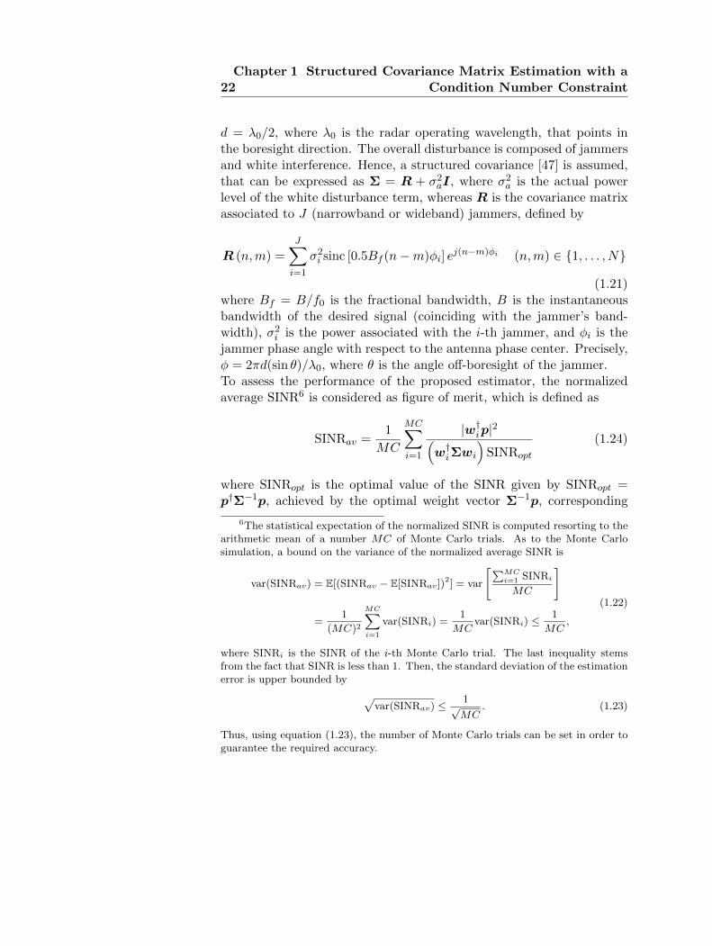
d = λ0/2, where λ0 is the radar operating wavelength, that points inthe boresight direction. The overall disturbance is composed of jammersand white interference. Hence, a structured covariance [47] is assumed,that can be expressed as Σ = R + σ2
aI, where σ2a is the actual power
level of the white disturbance term, whereas R is the covariance matrixassociated to J (narrowband or wideband) jammers, defined by
R (n,m) =
J∑i=1
σ2i sinc [0.5Bf (n−m)φi] e
j(n−m)φi (n,m) ∈ 1, . . . , N
(1.21)where Bf = B/f0 is the fractional bandwidth, B is the instantaneousbandwidth of the desired signal (coinciding with the jammer’s band-width), σ2
i is the power associated with the i-th jammer, and φi is thejammer phase angle with respect to the antenna phase center. Precisely,φ = 2πd(sin θ)/λ0, where θ is the angle off-boresight of the jammer.To assess the performance of the proposed estimator, the normalizedaverage SINR6 is considered as figure of merit, which is defined as
SINRav =1
MC
MC∑i=1
|w†ip|2(w†iΣwi
)SINRopt
(1.24)
where SINRopt is the optimal value of the SINR given by SINRopt =p†Σ−1p, achieved by the optimal weight vector Σ−1p, corresponding
6The statistical expectation of the normalized SINR is computed resorting to thearithmetic mean of a number MC of Monte Carlo trials. As to the Monte Carlosimulation, a bound on the variance of the normalized average SINR is
var(SINRav) = E[(SINRav − E[SINRav])2] = var
[∑MCi=1 SINRi
MC
]
=1
(MC)2
MC∑i=1
var(SINRi) =1
MCvar(SINRi) ≤
1
MC,
(1.22)
where SINRi is the SINR of the i-th Monte Carlo trial. The last inequality stemsfrom the fact that SINR is less than 1. Then, the standard deviation of the estimationerror is upper bounded by √
var(SINRav) ≤ 1√MC
. (1.23)
Thus, using equation (1.23), the number of Monte Carlo trials can be set in order toguarantee the required accuracy.
1.3 Performance Analysis 23
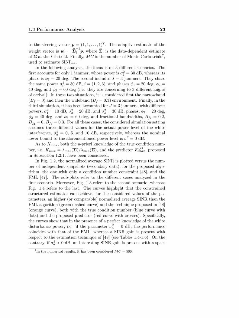
to the steering vector p = (1, 1, . . . , 1)T . The adaptive estimate of the
weight vector is wi = Σ−1
i p, where Σi is the data-dependent estimateof Σ at the i-th trial. Finally, MC is the number of Monte Carlo trials7,used to estimate SINRav.
In the following analysis, the focus is on 3 different scenarios. Thefirst accounts for only 1 jammer, whose power is σ2
1 = 30 dB, whereas itsphase is φ1 = 20 deg. The second includes J = 3 jammers. They sharethe same power σ2
i = 30 dB, i = (1, 2, 3), and phases φ1 = 20 deg, φ2 =40 deg, and φ3 = 60 deg (i.e. they are concerning to 3 different anglesof arrival). In these two situations, it is considered first the narrowband(Bf = 0) and then the wideband (Bf = 0.3) environment. Finally, in thethird simulation, it has been accounted for J = 3 jammers, with differentpowers, σ2
1 = 10 dB, σ22 = 20 dB, and σ2
3 = 30 dB, phases, φ1 = 20 deg,φ2 = 40 deg, and φ3 = 60 deg, and fractional bandwidths, Bf1 = 0.2,Bf2 = 0, Bf3 = 0.3. For all these cases, the considered simulation settingassumes three different values for the actual power level of the whiteinterference, σ2
a = 0, 5, and 10 dB, respectively, whereas the nominallower bound to the aforementioned power level is σ2 = 0 dB.
As to Kmax, both the a-priori knowledge of the true condition num-
ber, i.e. Kmax = λmax(Σ)/λmin(Σ), and the predictor K(∗)max, proposed
in Subsection 1.2.1, have been considered.
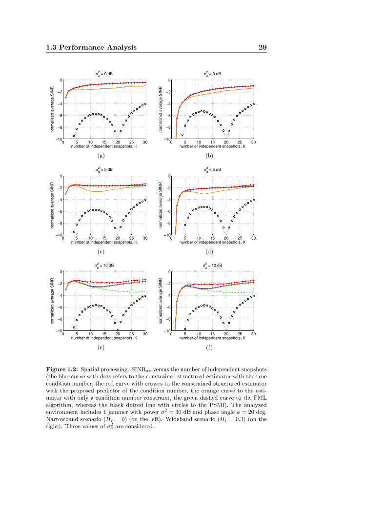
In Fig. 1.2, the normalized average SINR is plotted versus the num-ber of independent snapshots (secondary data), for the proposed algo-rithm, the one with only a condition number constraint [48], and theFML [47]. The sub-plots refer to the different cases analyzed in thefirst scenario. Moreover, Fig. 1.3 refers to the second scenario, whereasFig. 1.4 refers to the last. The curves highlight that the constrainedstructured estimator can achieve, for the considered values of the pa-rameters, an higher (or comparable) normalized average SINR than theFML algorithm (green dashed curve) and the technique proposed in [48](orange curve), both with the true condition number (blue curve withdots) and the proposed predictor (red curve with crosses). Specifically,the curves show that in the presence of a perfect knowledge of the whitedisturbance power, i.e. if the parameter σ2
a = 0 dB, the performancecoincides with that of the FML, whereas a SINR gain is present withrespect to the estimation technique of [48] (see Tables 1.4-1.6). On thecontrary, if σ2
a > 0 dB, an interesting SINR gain is present with respect
7In the numerical results, it has been considered MC = 500.
24Chapter 1 Structured Covariance Matrix Estimation with a
Condition Number Constraint
to the FML (as shown in Tables 1.1-1.3)8. In particular, the proposedestimator with the proposed predictor of Kmax exhibits a SINR gain of1.8 dB with respect to the FML, in the presence of 3 wideband jammersand with 10 dB power level of the white interference. Furthermore, theproposed estimator exhibits a SINR gain of 0.9 dB with respect to thealgorithm of [48], in the presence of 3 narrowband jammers and with 0dB power level of the white interference. Notice that, for comparisonpurpose, the PSMI (Pseudo Sample Matrix Inverse) is also considered inthe simulations of Figs. 1.2, 1.3, and 1.4 (black dotted line with circles).In particular, the PSMI [4] computes the inverse of the sample covari-ance matrix when the condition K ≥ N holds true; conversely, it utilizesthe pseudo inverse of the sample matrix when K < N . As expected, thecurves show a severe performance degradation of the PSMI with respectto all the other analyzed algorithms; however, it can be seen that asN increases (in particular for K >> N) the performance of the PSMItends to reach those of the other algorithms herein considered.
Table 1.1: Maximum SINR gain (in dB) of the proposed estimator, both with thetrue condition number and its proposed predictor, with respect to the FML. Thevalues refer to the simulations of Fig. 1.2.
case 1.2a 1.2b 1.2c 1.2d 1.2e 1.2f
true Kmax 0 0 0 0 1.7 1.6
K(∗)max 0 0 0.3 0.3 2 1.9
In Fig. 1.5, the effect of Kmax on the jammer cancellation and itsconnection with the required processor wordlength, [7], is shown for somevalues of K, assuming a power level of the white disturbance σ2
a = 0 dB,and the presence of 1 narrowband jammer with power σ2
1 = 30 dB anda phase angle φ = 25 deg (100 Monte Carlo independent trials havebeen considered). Therein, the average Output Response Ratio (ORR)is plotted, i.e. the average ratio between the squared modulus of the
8Notice that, if dN ≥ 1, then the proposed estimator coincides with the es-timator which accounts only for a condition number constraint. Moreover, sinceσ2a + λmin (R) = λmin (E [S]) ≥ E [λmin (S)] = E [dmin], where the upper bound be-
comes tighter and tighter as K increases, it is expected that the probability that theminimum eigenvalue is less than 1 increases as long as σ2
a + λmin (R) is close to 1.This explains the results obtained in the simulations, i.e. a SINR gain is obtained inthe presence of narrowband jammers and σ2
a = 1, when the smallest eigenvalue of thetrue covariance matrix is equal to 1.
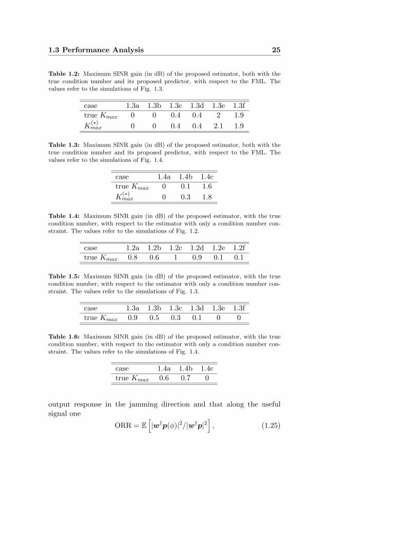
1.3 Performance Analysis 25
Table 1.2: Maximum SINR gain (in dB) of the proposed estimator, both with thetrue condition number and its proposed predictor, with respect to the FML. Thevalues refer to the simulations of Fig. 1.3.
case 1.3a 1.3b 1.3c 1.3d 1.3e 1.3f
true Kmax 0 0 0.4 0.4 2 1.9
K(∗)max 0 0 0.4 0.4 2.1 1.9
Table 1.3: Maximum SINR gain (in dB) of the proposed estimator, both with thetrue condition number and its proposed predictor, with respect to the FML. Thevalues refer to the simulations of Fig. 1.4.
case 1.4a 1.4b 1.4c
true Kmax 0 0.1 1.6
K(∗)max 0 0.3 1.8
Table 1.4: Maximum SINR gain (in dB) of the proposed estimator, with the truecondition number, with respect to the estimator with only a condition number con-straint. The values refer to the simulations of Fig. 1.2.
case 1.2a 1.2b 1.2c 1.2d 1.2e 1.2f
true Kmax 0.8 0.6 1 0.9 0.1 0.1
Table 1.5: Maximum SINR gain (in dB) of the proposed estimator, with the truecondition number, with respect to the estimator with only a condition number con-straint. The values refer to the simulations of Fig. 1.3.
case 1.3a 1.3b 1.3c 1.3d 1.3e 1.3f
true Kmax 0.9 0.5 0.3 0.1 0 0
Table 1.6: Maximum SINR gain (in dB) of the proposed estimator, with the truecondition number, with respect to the estimator with only a condition number con-straint. The values refer to the simulations of Fig. 1.4.
case 1.4a 1.4b 1.4c
true Kmax 0.6 0.7 0
output response in the jamming direction and that along the usefulsignal one
ORR = E[|w†p(φ)|2/|w†p|2
], (1.25)
26Chapter 1 Structured Covariance Matrix Estimation with a
Condition Number Constraint
where p(φ) = [1, exp(jφ), exp(2jφ), . . . , exp((N − 1)jφ)]T is the steering
vector in the direction φ and w = Σ−1p. Evidently, the smaller the
available number of bit nb = dlog2Kmaxe [7, equation 4.102a p. 156],the worse the cancellation capabilities of the processor. This can beexplained observing that the dynamic range of the eigenvalues in theestimated covariance matrix decreases as Kmax decreases. As a conse-quence, the processor tends to treat all the directions in the same wayor, equivalently, it has less degrees of freedom to set the depth of the nullalong the interference direction. Another implication of the eigenvaluesdynamic range reduction (ruled by Kmax) is a stabilization of the pro-cessor angular response. Otherwise stated, the statistical realizations ofoutput angular pattern exhibit less and less fluctuations as Kmax de-creases. This is an important feature in practical applications becausewith a quite stable pattern, the disturbance is not very sensible to themodulation resulting from the spatial adaptivity; hence, it could be alsocancelled with standard techniques like Moving Target Indicator (MTI)or extensions.
1.3.2 Doppler Processing in the Presence of Bimodal Clut-ter plus White Noise
The bimodal clutter model accounts for the presence of statisticallyindependent ground and sea clutters in addition to the white noise.Assuming a Gaussian shaped PSD [80] for both the interfering sources,the (i, k)-th element of the overall normalized disturbance covariancematrix is given by
Σ(i, k) = CNRSρ(i−k)2
S exp [−j2π(i− k)fS ] + CNRGρ(i−k)2
G
+ σ2aδi,k,
(1.26)
where CNRS and CNRG denote respectively the Clutter to Noise powerRatio for the sea and the ground clutter, ρS and ρG are respectivelythe one-lag correlation coefficients for the sea and the ground clutter,fS is the normalized Doppler frequency of the sea clutter, and δi,k isthe Kronecker delta function. The performance assessments for thecase of Doppler processing refer to 3 different cases, where the actualpower level of the white interference σ2
a assumes, respectively, the val-
1.3 Performance Analysis 27
ues 0, 5, 10 dB9. The considered temporal steering vector is given byp = [1, exp(j2πfd), . . . , exp(j2π(N − 1)fd)]
T , with fd = 0.15. Othersimulations parameters are specified in the captions of Figs. 1.6 and1.7.
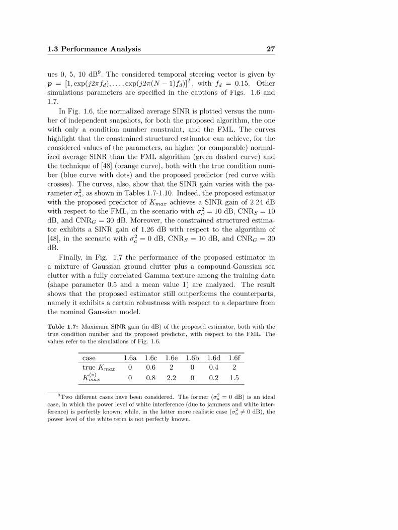
In Fig. 1.6, the normalized average SINR is plotted versus the num-ber of independent snapshots, for both the proposed algorithm, the onewith only a condition number constraint, and the FML. The curveshighlight that the constrained structured estimator can achieve, for theconsidered values of the parameters, an higher (or comparable) normal-ized average SINR than the FML algorithm (green dashed curve) andthe technique of [48] (orange curve), both with the true condition num-ber (blue curve with dots) and the proposed predictor (red curve withcrosses). The curves, also, show that the SINR gain varies with the pa-rameter σ2
a, as shown in Tables 1.7-1.10. Indeed, the proposed estimatorwith the proposed predictor of Kmax achieves a SINR gain of 2.24 dBwith respect to the FML, in the scenario with σ2
a = 10 dB, CNRS = 10dB, and CNRG = 30 dB. Moreover, the constrained structured estima-tor exhibits a SINR gain of 1.26 dB with respect to the algorithm of[48], in the scenario with σ2
a = 0 dB, CNRS = 10 dB, and CNRG = 30dB.
Finally, in Fig. 1.7 the performance of the proposed estimator ina mixture of Gaussian ground clutter plus a compound-Gaussian seaclutter with a fully correlated Gamma texture among the training data(shape parameter 0.5 and a mean value 1) are analyzed. The resultshows that the proposed estimator still outperforms the counterparts,namely it exhibits a certain robustness with respect to a departure fromthe nominal Gaussian model.
Table 1.7: Maximum SINR gain (in dB) of the proposed estimator, both with thetrue condition number and its proposed predictor, with respect to the FML. Thevalues refer to the simulations of Fig. 1.6.
case 1.6a 1.6c 1.6e 1.6b 1.6d 1.6f
true Kmax 0 0.6 2 0 0.4 2
K(∗)max 0 0.8 2.2 0 0.2 1.5
9Two different cases have been considered. The former (σ2a = 0 dB) is an ideal
case, in which the power level of white interference (due to jammers and white inter-ference) is perfectly known; while, in the latter more realistic case (σ2
a 6= 0 dB), thepower level of the white term is not perfectly known.
28Chapter 1 Structured Covariance Matrix Estimation with a
Condition Number Constraint
Table 1.8: Maximum SINR gain (in dB) of the proposed estimator, both with thetrue condition number and its proposed predictor, with respect to the FML. Thevalues refer to the simulations of Fig. 1.7.
case 1.7a 1.7c 1.7e 1.7b 1.7d 1.7f
true Kmax 0 0.5 1.9 0 0.4 2
K(∗)max 0 0.8 2.2 0 0.2 1.5
Table 1.9: Maximum SINR gain (in dB) of the proposed estimator, with the truecondition number, with respect to the estimator with only a condition number con-straint. The values refer to the simulations of Fig. 1.6.
case 1.6a 1.6c 1.6e 1.6b 1.6d 1.6f
true Kmax 1.3 0.5 0 1.2 0.6 0
Table 1.10: Maximum SINR gain (in dB) of the proposed estimator, with thetrue condition number, with respect to the estimator with only a condition numberconstraint. The values refer to the simulations of Fig. 1.7.
case 1.7a 1.7c 1.7e 1.7b 1.7d 1.7f
true Kmax 1.2 0.5 0 1.2 0.6 0
1.3 Performance Analysis 29
0 5 10 15 20 25 30−10
−8
−6
−4
−2
0
σa
2 = 0 dB
number of independent snapshots, K
no
rma
lize
d a
ve
rag
e S
INR
(a)
0 5 10 15 20 25 30−10
−8
−6
−4
−2
0
σa
2 = 0 dB
number of independent snapshots, K
no
rma
lize
d a
ve
rag
e S
INR
(b)
0 5 10 15 20 25 30−10
−8
−6
−4
−2
0
σa
2 = 5 dB
number of independent snapshots, K
no
rma
lize
d a
ve
rag
e S
INR
(c)
0 5 10 15 20 25 30−10
−8
−6
−4
−2
0
σa
2 = 5 dB
number of independent snapshots, K
no
rma
lize
d a
ve
rag
e S
INR
(d)
0 5 10 15 20 25 30−10
−8
−6
−4
−2
0
σa
2 = 10 dB
number of independent snapshots, K
no
rma
lize
d a
ve
rag
e S
INR
(e)
0 5 10 15 20 25 30−10
−8
−6
−4
−2
0
σa
2 = 10 dB
number of independent snapshots, K
no
rma
lize
d a
ve
rag
e S
INR
(f)
Figure 1.2: Spatial processing. SINRav versus the number of independent snapshots(the blue curve with dots refers to the constrained structured estimator with the truecondition number, the red curve with crosses to the constrained structured estimatorwith the proposed predictor of the condition number, the orange curve to the esti-mator with only a condition number constraint, the green dashed curve to the FMLalgorithm, whereas the black dotted line with circles to the PSMI). The analyzedenvironment includes 1 jammer with power σ2 = 30 dB and phase angle φ = 20 deg.Narrowband scenario (Bf = 0) (on the left). Wideband scenario (Bf = 0.3) (on theright). Three values of σ2
a are considered.
30Chapter 1 Structured Covariance Matrix Estimation with a
Condition Number Constraint
0 5 10 15 20 25 30−15
−10
−5
0
σa
2 = 0 dB
number of independent snapshots, K
no
rma
lize
d a
ve
rag
e S
INR
(a)
5 10 15 20 25 30−10
−8
−6
−4
−2
0
σa
2 = 0 dB
number of independent snapshots, K
no
rma
lize
d a
ve
rag
e S
INR
(b)
0 5 10 15 20 25 30−15
−10
−5
0
σa
2 = 5 dB
number of independent snapshots, K
no
rma
lize
d a
ve
rag
e S
INR
(c)
0 5 10 15 20 25 30−15
−10
−5
0
σa
2 = 5 dB
number of independent snapshots, K
no
rma
lize
d a
ve
rag
e S
INR
(d)
0 5 10 15 20 25 30−15
−10
−5
0
σa
2 = 10 dB
number of independent snapshots, K
no
rma
lize
d a
ve
rag
e S
INR
(e)
0 5 10 15 20 25 30−15
−10
−5
0
σa
2 = 10 dB
number of independent snapshots, K
no
rma
lize
d a
ve
rag
e S
INR
(f)
Figure 1.3: Spatial processing. SINRav versus the number of independent snap-shots (the blue curve with dots refers to the constrained structured estimator withthe true condition number, the red curve with crosses to the constrained structuredestimator with the proposed predictor of the condition number, the orange curve tothe estimator with only a condition number constraint, the green dashed curve tothe FML algorithm, whereas the black dotted line with circles to the PSMI). Theanalyzed environment includes 3 jammers with power σ2 = 30 dB and phase angles(φ1, φ2, φ3) = (20, 40, 60) deg. Narrowband scenario (Bf = 0) (on the left). Wide-band scenario (Bf = 0.3) (on the right). Three values of σ2
a are considered.
1.3 Performance Analysis 31
0 5 10 15 20 25 30−15
−10
−5
0
σa
2 = 0 dB
number of independent snapshots, K
no
rma
lize
d a
ve
rag
e S
INR
(a)
0 5 10 15 20 25 30−15
−10
−5
0
σa
2 = 5 dB
number of independent snapshots, K
no
rma
lize
d a
ve
rag
e S
INR
(b)
0 5 10 15 20 25 30−15
−10
−5
0
σa
2 = 10 dB
number of independent snapshots, K
no
rma
lize
d a
ve
rag
e S
INR
(c)
Figure 1.4: Spatial processing. SINRav versus the number of independent snapshots(the blue curve with dots refers to the constrained structured estimator with the truecondition number, the red curve with crosses to the constrained structured estimatorwith the proposed predictor of the condition number, the orange curve to the esti-mator with only a condition number constraint, the green dashed curve to the FMLalgorithm, whereas the black dotted line with circles to the PSMI). The analyzedenvironment includes 3 jammers with powers (σ2
1 , σ22 , σ
23) = (10, 20, 30) dB, phase
angles (φ1, φ2, φ3) = (20, 40, 60) deg and fractional bandwidth Bf = (0.2, 0, 0.3),respectively. Three values of σ2
a are considered.
32Chapter 1 Structured Covariance Matrix Estimation with a
Condition Number Constraint
0 5 10 15−70
−60
−50
−40
−30
−20
−10
nb
OR
R [
dB
] K=10K=20
K=40 K=60
Figure 1.5: Spatial processing. Average ORR (expressed in dB) versusdlog2(Kmax)e, which is the minimum required wordlength. The analyzed environ-ment includes 1 narrowband jammer with power σ2
1 = 30 dB and phase angle φ = 25deg. The analysis has been conducted for different values of the sample support (i.e.K = N/2, K = N , K = 2N , and K = 3N).
1.3 Performance Analysis 33
0 5 10 15 20 25 30−16
−14
−12
−10
−8
−6
−4
−2
σa
2 = 0 dB
number of independent snapshots, K
no
rma
lize
d a
ve
rag
e S
INR
(a)
0 5 10 15 20 25 30−4
−3.5
−3
−2.5
−2
−1.5
σa
2 = 0 dB
number of independent snapshots, K
no
rma
lize
d a
ve
rag
e S
INR
(b)
0 5 10 15 20 25 30−14
−12
−10
−8
−6
−4
−2
σa
2 = 5 dB
number of independent snapshots, K
no
rma
lize
d a
ve
rag
e S
INR
(c)
0 5 10 15 20 25 30
−3
−2.5
−2
−1.5
σa
2 = 5 dB
number of independent snapshots, K
no
rma
lize
d a
ve
rag
e S
INR
(d)
0 5 10 15 20 25 30−10
−8
−6
−4
−2
σa
2 = 10 dB
number of independent snapshots, K
no
rma
lize
d a
ve
rag
e S
INR
(e)
0 5 10 15 20 25 30−4
−3.5
−3
−2.5
−2
−1.5
−1
−0.5
σa
2 = 10 dB
number of independent snapshots, K
no
rma
lize
d a
ve
rag
e S
INR
(f)
Figure 1.6: Doppler processing. SINRav versus the number of independent snap-shots (the blue curve with dots refers to the constrained structured estimator withthe true condition number, the red curve with crosses to the constrained structuredestimator with the proposed predictor of the condition number, the orange curve tothe estimator with only a condition number constraint, whereas the green dashedcurve to the FML algorithm). The analyzed environment parameters are ρS = 0.6dB, ρG = 0.99, fS = 0.2, and CNRS = 10 dB and CNRG = 30 dB for the curves onthe left, and CNRS = 5 dB and CNRG = 10 dB for the curves on the right. Threevalues of σ2
a are considered.
34Chapter 1 Structured Covariance Matrix Estimation with a
Condition Number Constraint
0 5 10 15 20 25 30−16
−14
−12
−10
−8
−6
−4
−2
σa
2 = 0 dB
number of snapshots, K
no
rma
lize
d a
ve
rag
e S
INR
(a)
0 5 10 15 20 25 30
−3.5
−3
−2.5
−2
σa
2 = 0 dB
number of snapshots, K
no
rma
lize
d a
ve
rag
e S
INR
(b)
0 5 10 15 20 25 30−14
−12
−10
−8
−6
−4
−2
σa
2 = 5 dB
number of snapshots, K
no
rma
lize
d a
ve
rag
e S
INR
(c)
0 5 10 15 20 25 30
−3
−2.5
−2
−1.5
σa
2 = 5 dB
number of snapshots, K
no
rma
lize
d a
ve
rag
e S
INR
(d)
0 5 10 15 20 25 30−10
−8
−6
−4
−2
σa
2 = 10 dB
number of snapshots, K
no
rma
lize
d a
ve
rag
e S
INR
(e)
0 5 10 15 20 25 30−4
−3.5
−3
−2.5
−2
−1.5
−1
−0.5
σa
2 = 10 dB
number of snapshots, K
no
rma
lize
d a
ve
rag
e S
INR
(f)
Figure 1.7: Doppler processing. SINRav versus the number of snapshots (the bluecurve with dots refers to the constrained structured estimator with the true conditionnumber, the red curve with crosses to the constrained structured estimator with theproposed predictor of the condition number, the orange curve to the estimator withonly a condition number constraint, whereas the green dashed curve to the FMLalgorithm). The analyzed environment parameters are ρS = 0.6 dB, ρG = 0.99,fS = 0.2, and CNRS = 10 dB and CNRG = 30 dB for the curves on the left, andCNRS = 5 dB and CNRG = 10 dB for the curves on the right. Gamma texture shapeparameter 0.5 and mean value 1. Three values of σ2
a are considered.
Chapter 2
Geometric Approaches toCovariance Estimation forSecondary Data Selection
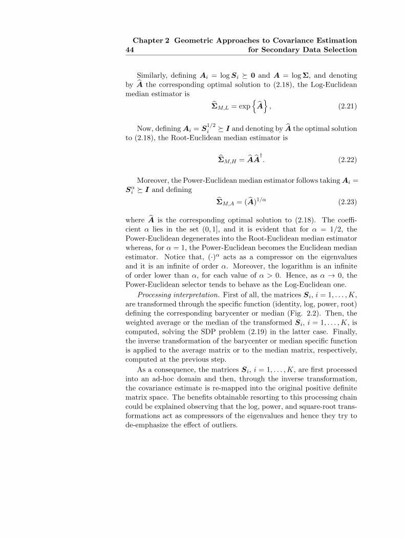
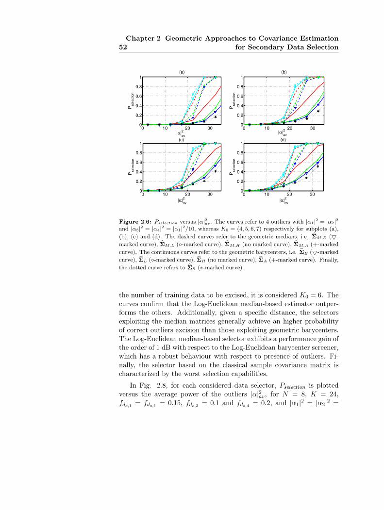
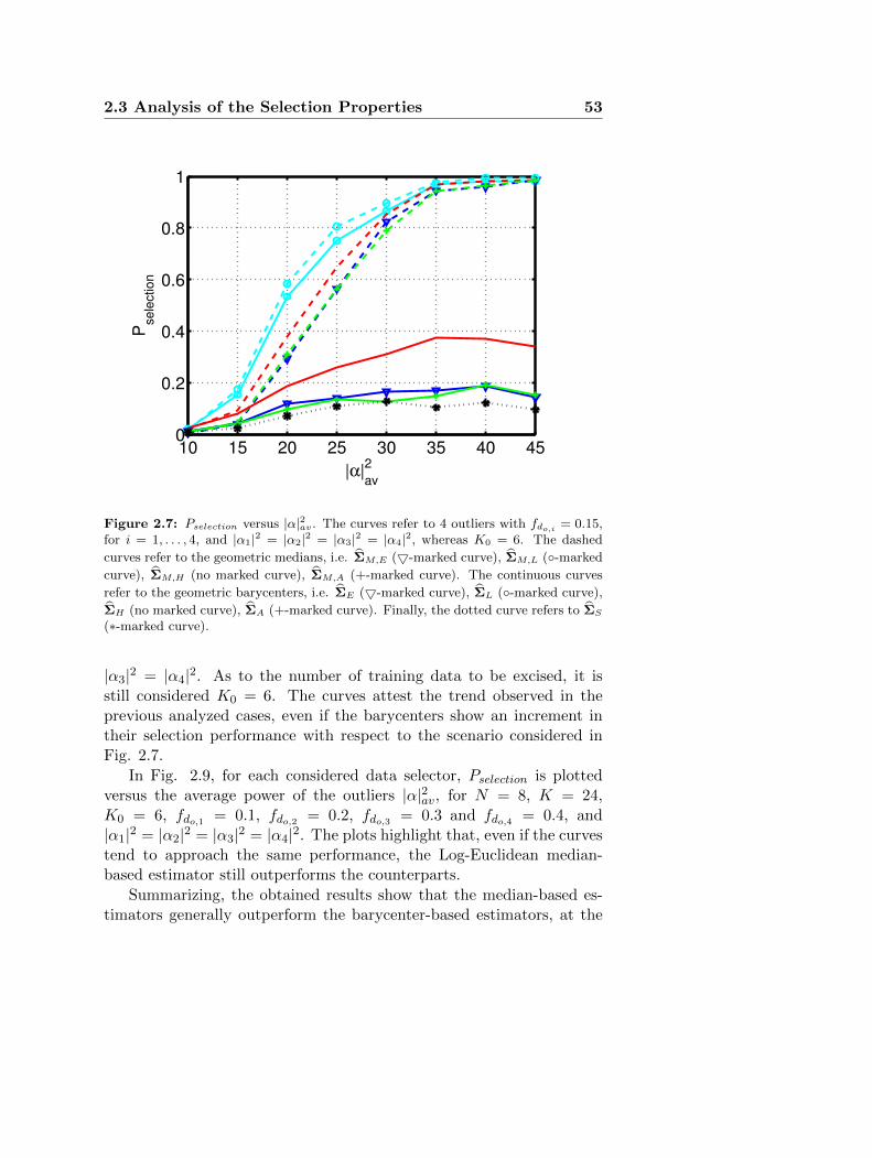
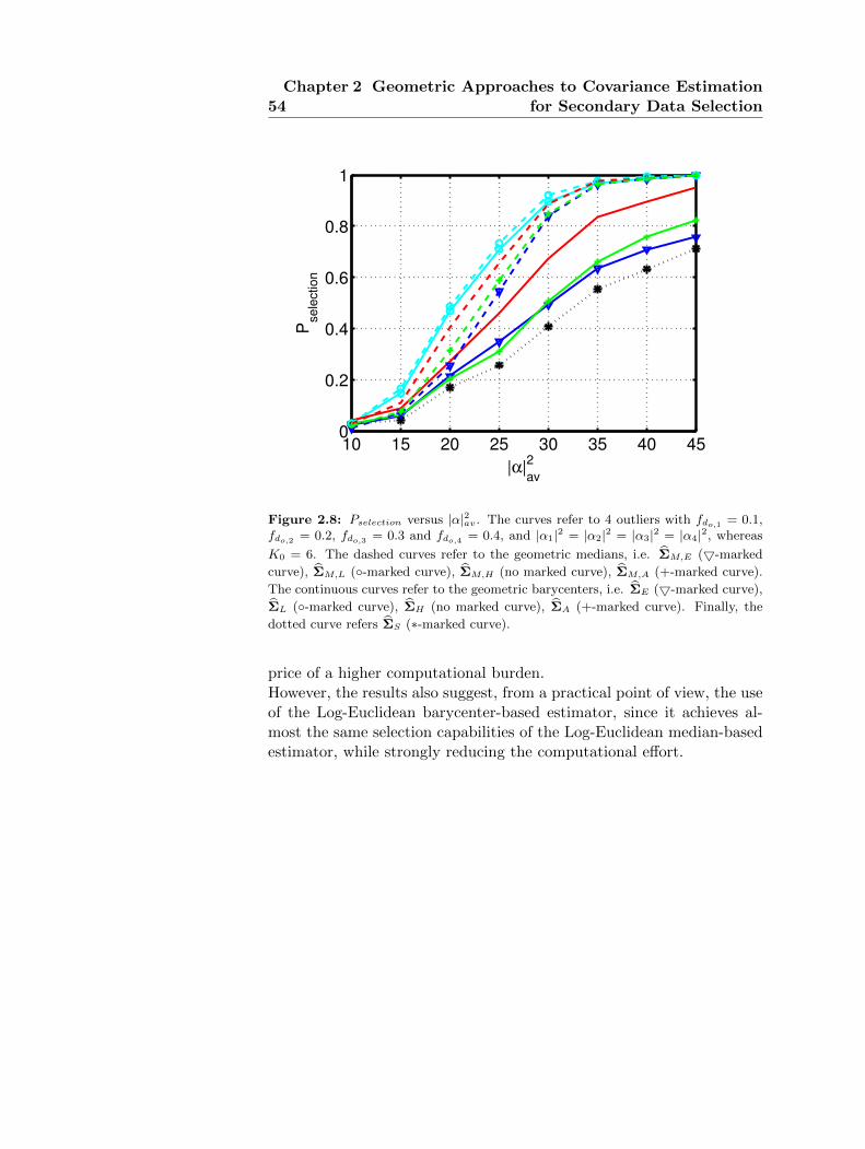
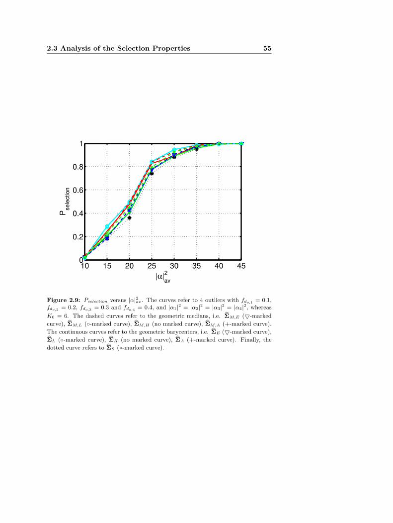
In this chapter, two classes of covariance matrix estimators whichdoes not depend on the probability distribution function of the samplesupport are proposed and analyzed. Precisely, any estimator of thesetwo classes is associated to a suitable distance in the considered spaceand is defined, respectively, as the median matrix [23] or the geomet-ric barycenter [81] of a set of covariance matrices, obtained from theavailable secondary data set. As to the considered distances, the focusis on Euclidean, Log-Euclidean, Root-Euclidean, and Power-Euclideandistances [82]. Furthermore, the basic covariance matrix estimates (usedin the matrix median and geometric barycenter calculations) are com-puted exploiting some a-priori information about the covariance matrixstructure [83]. Based on the new devised estimators, training data selec-tors, whose aim is to discard secondary data containing outliers, are pro-posed. The selection is based on the Generalized Inner Product (GIP)[8] exploiting the median matrices or the geometric barycenters in placeof the classic sample covariance matrix.
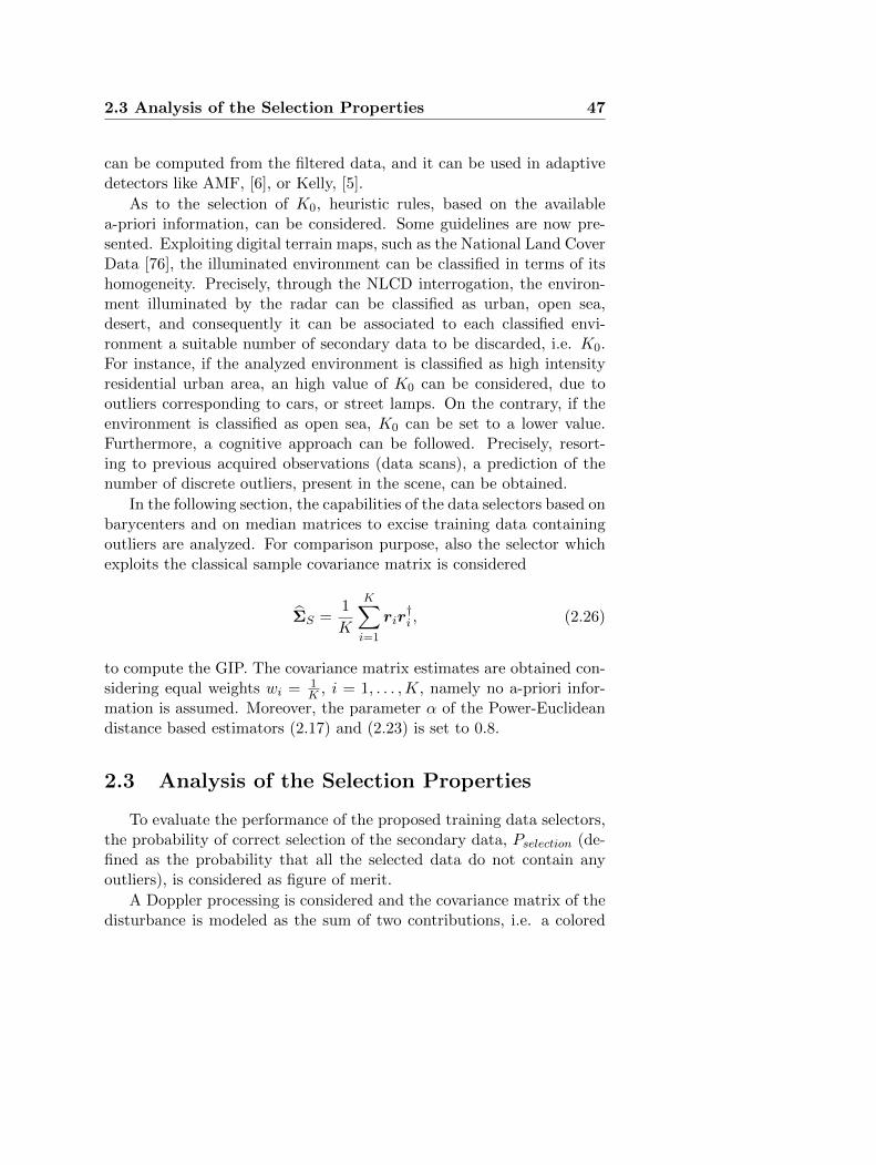
At the analysis level, the performance of the new selection schemesare assessed, in terms of probability of correct outliers excision, compar-ing the systems exploiting the geometric barycenters with those exploit-ing the median matrices. The results show that data selectors exploitinggeometric medians can outperform those based on geometric barycen-
35
36Chapter 2 Geometric Approaches to Covariance Estimation
for Secondary Data Selection
ters but the former require a computational complexity higher than thelatter.
The chapter is organized as follows. In Section 2.1, the system modelis described and the two families of estimators are presented; the for-mer are obtained as the solution of a convex optimization problem (i.e.the median matrices) and the latter are obtained in a closed form. InSection 2.2, training data selectors are presented, whereas in Section 2.3performance analysis are provided.
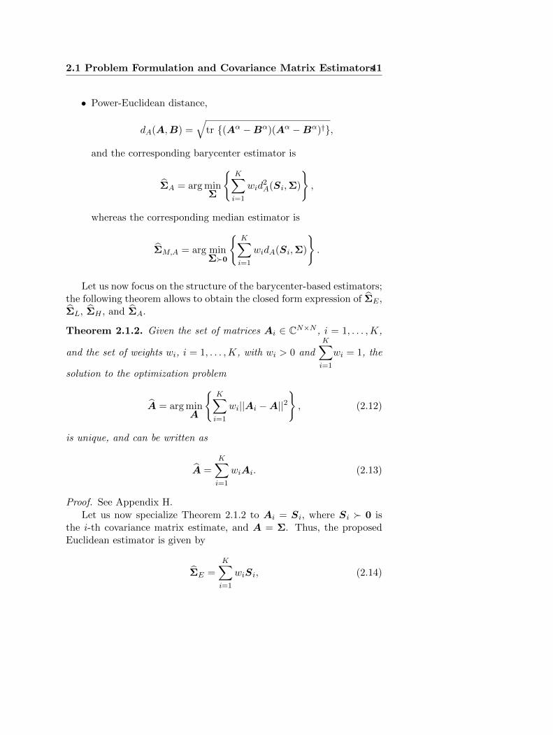
2.1 Problem Formulation and Covariance Ma-trix Estimators
This section formalizes the problem of estimating the positive definitecovariance matrix Σ, of K secondary data r1, . . . , rK , modeled as N -dimensional circularly symmetric zero-mean vectors, with an arbitraryjoint statistical distribution, and sharing the same covariance matrix
E[rir†i
]= Σ, i = 1, . . . ,K, (2.1)
assumed positive definite.
When the statistical characterization of the secondary data is notknown, classic approaches, such as the ML or the Minimum Mean SquareError (MMSE) estimations, cannot be applied, and different families ofcovariance matrix estimators must be introduced.
The framework proposed in this chapter relies on the use of suitabletypes of distances in the positive definite matrix space, namely on thecone of the positive definite matrices as illustrated in Fig. 2.1. Otherwise
Figure 2.1: Cone of positive definite matrices.
2.1 Problem Formulation and Covariance Matrix Estimators37
stated, two classes of estimators are defined, based respectively on thegeometric barycenter and the generalized median matrix of a set of basiccovariance matrix estimates, obtained from the available secondary dataset. Specifically, denoting by Si, i = 1, . . . ,K, the set of basic covariancematrix estimates and given a distance
d(·, ·) : A 0,B 0→ [0,+∞),
the corresponding geometric barycenter-based estimator is defined as
Σ = arg minΣ0
K∑i=1
wid2(Si,Σ)
, (2.2)
whereas the median-based estimator is
ΣM = arg minΣ0
K∑i=1
wid(Si,Σ)
. (2.3)
Notice that, the coefficients wi (with wi > 0 and∑K
i=1wi = 1) allowto weight the secondary data, in order to account for their reliability,for instance their degree of homogeneity or temporal acquisition. Theweights, wi, can be also chosen on the basis of the similarity between thesecondary data terrain and that of the cell under test (exploiting, for in-stance, the so-called National Land Cover Data, NLCD [76]). Of course,without any source of a-priori knowledge, it is reasonable to set equalweights and ΣM ends up coincident with the median matrix induced bythe metric d(·, ·) of the set of matrices Si, i = 1, . . . ,K. Moreover, whenwi = 1/K, i = 1, . . . ,K, and the matrices Si are assumed i.i.d. randompositive definite matrix, then
Σ = arg minΣ
1
K
K∑i=1
d2(Si,Σ)
,
is an empirical (sample) Frechet mean [84], [85], where a Frechet meanof an N ×N random covariance matrix S is given by [84], [85]
Ω = arg minΩ
E[d2(S,Ω)
]. (2.4)
The idea of using the generalized median matrix in (2.3) stems fromthe well known robustness of the conventional median value with respect
38Chapter 2 Geometric Approaches to Covariance Estimation
for Secondary Data Selection
to the presence of outliers in the data. To better explain this concept,it can be recalled that the median value of a real random variable X isdefined as
x = arg minm
E [|X −m|] , with m ∈ R. (2.5)
It is well known that, for a continuous random variable, x is such that
Pr (X ≤ x) =1
2(2.6)
namely, the conventional median corresponds to the 50% percentile ofthe distribution of x. Let us now observe that for an empirical distribu-tion defined by a set of real observations xi, i = 1, . . . , N0, the empiricalmedian value is given by
xe = arg minm
1
N0
N0∑i=1
|xi −m|, with m ∈ R. (2.7)
Thus, denoting by x(i), i = 1, . . . , N0 the ordered observations in increas-ing order, it is easy to show that xe = x(dN2 e)
. Consequently, replacing
an observation xi > x with another (possibly much higher) y > x, thenew empirical median value does not change. In other words, there is arobustness of the median with respect to the presence of outliers. There-fore, leveraging on the above consideration and exploiting the conceptof median matrix, which is a generalization of classic median definition,it is possible to devise robust covariance matrix estimators.
As to the set of basic covariance matrix estimates, it is assumed thateach Si is a function of the single secondary datum ri, namely Si =Si(ri), i = 1, . . . ,K. In particular, a possible choice could be the rank-
one sample matrix related to the vector ri, namely Si = rir†i . However,
this is not acceptable since the aforementioned definition of distancerequires that the considered matrices are positive definite; hence a-prioriinformation has to be exploited to come up with positive definiteness.Toward this goal, the knowledge of a lower bound to the spectral densityof the white noise is assumed (set, without loss of generality, to 0 dB),and the covariance matrix which minimizes the Euclidean distance (also
called Frobenius distance) from rir†i is associated to each vector of the
sample support, under the constraint Si I. The following theorem,provides the explicit expression of the aforementioned minimizer.
2.1 Problem Formulation and Covariance Matrix Estimators39
Theorem 2.1.1. Let ri be the i-th N -dimensional secondary datum, thematrix Si which minimizes the Frobenius distance from rir
†i under the
constraint Si I, i.e. the optimal solution to the optimization problem
and U i is a unitary matrix of the eigenvectors of rir†i with the first
eigenvector corresponding to the eigenvalue ||ri||2.
Proof. See Appendix G.Notice that, the eigenvalue decomposition is not necessary to com-
pute (2.8) as
Si = rir†i max
([1− 1
||ri||2
], 0
)+ I. (2.11)
As shown in [83], the matrix Si in (2.9) also minimizes the distance
induced by the spectral norm from the matrix rir†i under the constraint
Si I. As to the considered distances, the focus is on the Euclidean,Log-Euclidean, Root-Euclidean, and Power-Euclidean distances. Thus,four covariance matrix estimators for each class are obtained, which arepresented in the next subsection.
2.1.1 Covariance Matrix Estimators based on GeometricBarycenters and Median Matrices
In this subsection, the considered distances are described, and thecorresponding estimators are derived. Specifically, let A 0 and B 0, the considered four distances and the corresponding estimators areformally defined as:
• Euclidean distance,
dE(A,B) =√
tr (A−B)(A−B)†,
40Chapter 2 Geometric Approaches to Covariance Estimation
for Secondary Data Selection
the corresponding barycenter estimator is
ΣE = arg minΣ
K∑i=1
wid2E(Si,Σ)
,
whereas the corresponding median estimator is
ΣM,E = arg minΣ0
K∑i=1
widE(Si,Σ)
.
• Log-Euclidean distance,
dL(A,B) =√
tr (logA− logB)(logA− logB)†,
the corresponding barycenter estimator is
ΣL = arg minΣ
K∑i=1
wid2L(Si,Σ)
,
whereas the corresponding median estimator is
ΣM,L = arg minΣ0
K∑i=1
widL(Si,Σ)
.
• Root-Euclidean distance,
dH(A,B) =
√tr
(A1/2 −B1/2
)(A1/2 −B1/2
)†,
and the corresponding barycenter estimator is
ΣH = arg minΣ
K∑i=1
wid2H(Si,Σ)
,
whereas the corresponding median estimator is
ΣM,H = arg minΣ0
K∑i=1
widH(Si,Σ)
.
2.1 Problem Formulation and Covariance Matrix Estimators41
• Power-Euclidean distance,
dA(A,B) =√
tr (Aα −Bα)(Aα −Bα)†,
and the corresponding barycenter estimator is
ΣA = arg minΣ
K∑i=1
wid2A(Si,Σ)
,
whereas the corresponding median estimator is
ΣM,A = arg minΣ0
K∑i=1
widA(Si,Σ)
.
Let us now focus on the structure of the barycenter-based estimators;the following theorem allows to obtain the closed form expression of ΣE ,ΣL, ΣH , and ΣA.
Theorem 2.1.2. Given the set of matrices Ai ∈ CN×N , i = 1, . . . ,K,
and the set of weights wi, i = 1, . . . ,K, with wi > 0 and
K∑i=1
wi = 1, the
solution to the optimization problem
A = arg minA
K∑i=1
wi||Ai −A||2, (2.12)
is unique, and can be written as
A =
K∑i=1
wiAi. (2.13)
Proof. See Appendix H.
Let us now specialize Theorem 2.1.2 to Ai = Si, where Si 0 isthe i-th covariance matrix estimate, and A = Σ. Thus, the proposedEuclidean estimator is given by
ΣE =
K∑i=1
wiSi, (2.14)
42Chapter 2 Geometric Approaches to Covariance Estimation
for Secondary Data Selection
namely, it is the weighted mean of the covariance matrix estimates, Si.For real numbers and wi = 1/K, i = 1, . . . ,K, this estimator becomesthe arithmetic mean.
Similarly, defining Ai = logSi and A = log Σ, the Log-Euclideanestimator can be expressed as
ΣL = exp
K∑i=1
wi logSi
, (2.15)
Notice that, for positive real numbers and wi = 1/K, i = 1, . . . ,K, ΣL
represents a generalization of the geometric mean1 of the matrices Si.
The Root-Euclidean estimator is obtained by substitutingAi = S1/2i
and A = ∆H = Σ1/2:
ΣH = ∆H∆†H where ∆H =
K∑i=1
wiS1/2i . (2.16)
Finally, the Power-Euclidean estimator follows, taking Ai = Sαi andA = ∆A = Σα, i.e.
ΣA = (∆A)1/α where ∆A =K∑i=1
wiSαi . (2.17)
The coefficient α usually lies in the set (0, 1], and it is obvious that forα = 1/2, the Power-Euclidean becomes the Root-Euclidean estimator,and for α = 1 it becomes the Euclidean one.
It can be explicitly observed that the estimators (2.16) and (2.17))extend to the positive definite matrix space the mean power definitionof a set of positive real numbers. Indeed, for positive numbers xi and
wi = 1/K, i = 1, . . . ,K, they reduce to(
1K
∑Ki=1 x
αi
)1/α, α ∈ (0, 1].
Let us now focus on the computation of the median-based estimators;the following theorems allow to obtain ΣM,E , ΣM,L, ΣM,H , and ΣM,A
from the solution of a convex optimization problem.
1Given K positive numbers (x1, x2, . . . , xK), the geometric mean, x =K√x1 · x2 · . . . · xK , minimizes the sum of the squared hyperbolic distances to the
given positive numbers xi:
x = arg minx>0
K∑i=1
| log x− log xi|2.
2.1 Problem Formulation and Covariance Matrix Estimators43
Theorem 2.1.3. Given the set of matrices Ai ∈ HN , i = 1, . . . ,K, and
the set of weights wi, i = 1, . . . ,K, with wi > 0 and
K∑i=1
wi = 1, the
matrix
A = arg minA∈HN
K∑i=1
wi||Ai −A||
, (2.18)
can be computed as the optimal solution to the convex optimizationSemidefinite Programming (SDP) problem
P1
min
t1,...,tK ,A
K∑i=1
witi
s.t.
(ti (vec(A)− vec(Ai))
†
(vec(A)− vec(Ai)) tiI
) 0
A ∈ HN
.
i = 1, . . . ,K
(2.19)
Proof. See Appendix I.
Notice that, the computational complexity connected with the solu-tion of the optimization problem P1 is O(N3.5 log(1/η)), where η is aprescribed accuracy (see [74]).
The following proposition provides an interesting property of themedian matrix in (2.18).
Proposition 2.1.4. If Ai 0, i = 1, . . . ,K, then A in (2.18) is positivesemidefinite. Moreover, if Ai 0, i = 1, . . . ,K, then A in (2.18) ispositive definite. Additionally, if the matrices Ai ∈ HN are not aligned,i.e. there are no Q0 ∈ HN and Q1 ∈ HN such that
Ai = tiQ1 +Q0, ti ∈ R, i = 1, . . . ,K, (2.20)
the median matrix is unique.
Proof. See Appendix J.
Let us now specialize Theorem 2.1.3 to Ai = Si, where Si I isthe i-th covariance matrix estimate, and A = Σ. Thus, the proposedEuclidean median estimator ΣM,E is obtained by the optimal solutionto (2.18).
44Chapter 2 Geometric Approaches to Covariance Estimation
for Secondary Data Selection
Similarly, defining Ai = logSi 0 and A = log Σ, and denotingby A the corresponding optimal solution to (2.18), the Log-Euclideanmedian estimator is
ΣM,L = expA, (2.21)
Now, definingAi = S1/2i I and denoting by A the optimal solution
to (2.18), the Root-Euclidean median estimator is
ΣM,H = AA†. (2.22)
Moreover, the Power-Euclidean median estimator follows takingAi =Sαi I and defining
ΣM,A = (A)1/α (2.23)
where A is the corresponding optimal solution to (2.18). The coeffi-cient α lies in the set (0, 1], and it is evident that for α = 1/2, thePower-Euclidean degenerates into the Root-Euclidean median estimatorwhereas, for α = 1, the Power-Euclidean becomes the Euclidean medianestimator. Notice that, (·)α acts as a compressor on the eigenvaluesand it is an infinite of order α. Moreover, the logarithm is an infiniteof order lower than α, for each value of α > 0. Hence, as α → 0, thePower-Euclidean selector tends to behave as the Log-Euclidean one.
Processing interpretation. First of all, the matrices Si, i = 1, . . . ,K,are transformed through the specific function (identity, log, power, root)defining the corresponding barycenter or median (Fig. 2.2). Then, theweighted average or the median of the transformed Si, i = 1, . . . ,K, iscomputed, solving the SDP problem (2.19) in the latter case. Finally,the inverse transformation of the barycenter or median specific functionis applied to the average matrix or to the median matrix, respectively,computed at the previous step.
As a consequence, the matrices Si, i = 1, . . . ,K, are first processedinto an ad-hoc domain and then, through the inverse transformation,the covariance estimate is re-mapped into the original positive definitematrix space. The benefits obtainable resorting to this processing chaincould be explained observing that the log, power, and square-root trans-formations act as compressors of the eigenvalues and hence they try tode-emphasize the effect of outliers.
2.2 Secondary Data Selection Design 45
Figure 2.2: A pictorial illustration about the generalized geometric barycen-ter/median computation procedure.
2.2 Secondary Data Selection Design
In the present section, a secondary data selection scheme exploit-ing the proposed barycenter and median-based covariance matrix esti-mators is introduced. The aim of the data selector is to choose themost homogeneous secondary data, discarding vectors containing possi-ble outliers. This screening is of paramount importance, since adaptivereceivers achieve satisfactory performances when the available secondarydata share the same spectral properties. In Fig. 2.3, the block-schemeof the proposed class of training data selectors is shown.
The selector screens among the K training data excising the K0
vectors with the highest GIP [8], [86], [87] computed using one of thenew devised covariance matrix estimators (described in Subsection 2.1.1)in place of the classic sample covariance matrix. Precisely, denotingby Ω = 1, 2, . . . ,K the set of the secondary data indices and byΩ0 = i1, i2, . . . , iK−K0 ⊆ Ω the subset, of cardinality K −K0, of the
46Chapter 2 Geometric Approaches to Covariance Estimation
for Secondary Data Selection
Figure 2.3: Pictorial representation of the training data selector scheme.
selected training data indices, the proposed screening procedure basedon the estimator Σd, where d accounts for the considered distance, canbe summarized as follows:
• compute the covariance matrix estimate Σd exploiting the sec-ondary data r1, r2, . . . , rK ;
• ∀ i ∈ Ω construct the quadratic form (GIP)
βdi = r†i Σ−1
d ri i = 1, . . . ,K, (2.24)
and sort βdi s in decreasing order;
• The set Ω0 of the selected K −K0 indices, is obtained censoringfrom Ω the indices corresponding to the K0 highest values βdi .
Notice that βdi measures the energy of the vector Σ− 1
2d ri. Thus, the
screening procedure excises the K0 data having the highest energy inthe “quasi-whitened-space”, where the whitening operation is tied up tothe specific covariance matrix estimate. Notice also that, the procedurehere illustrated is the same for the medians, substituting ΣM,d in place
of Σd.Whenever the secondary data have been selected, the sample covari-
ance matrix
ΣSM =1
K −K0
∑j∈Ω0
rjr†j (2.25)
2.3 Analysis of the Selection Properties 47
can be computed from the filtered data, and it can be used in adaptivedetectors like AMF, [6], or Kelly, [5].
As to the selection of K0, heuristic rules, based on the availablea-priori information, can be considered. Some guidelines are now pre-sented. Exploiting digital terrain maps, such as the National Land CoverData [76], the illuminated environment can be classified in terms of itshomogeneity. Precisely, through the NLCD interrogation, the environ-ment illuminated by the radar can be classified as urban, open sea,desert, and consequently it can be associated to each classified envi-ronment a suitable number of secondary data to be discarded, i.e. K0.For instance, if the analyzed environment is classified as high intensityresidential urban area, an high value of K0 can be considered, due tooutliers corresponding to cars, or street lamps. On the contrary, if theenvironment is classified as open sea, K0 can be set to a lower value.Furthermore, a cognitive approach can be followed. Precisely, resort-ing to previous acquired observations (data scans), a prediction of thenumber of discrete outliers, present in the scene, can be obtained.
In the following section, the capabilities of the data selectors based onbarycenters and on median matrices to excise training data containingoutliers are analyzed. For comparison purpose, also the selector whichexploits the classical sample covariance matrix is considered
ΣS =1
K
K∑i=1
rir†i , (2.26)
to compute the GIP. The covariance matrix estimates are obtained con-sidering equal weights wi = 1
K , i = 1, . . . ,K, namely no a-priori infor-mation is assumed. Moreover, the parameter α of the Power-Euclideandistance based estimators (2.17) and (2.23) is set to 0.8.
2.3 Analysis of the Selection Properties
To evaluate the performance of the proposed training data selectors,the probability of correct selection of the secondary data, Pselection (de-fined as the probability that all the selected data do not contain anyoutliers), is considered as figure of merit.
A Doppler processing is considered and the covariance matrix of thedisturbance is modeled as the sum of two contributions, i.e. a colored
48Chapter 2 Geometric Approaches to Covariance Estimation
for Secondary Data Selection
matrix accounting for the clutter and an identity matrix accounting forthe white thermal noise
Σ = Σ0 + I. (2.27)
Assuming a Gaussian shaped clutter PSD [80], the covariance matrixterm due to the clutter is modeled as
Σ0(i, k) = σ2cρ|i−k|ej2πfdc (i−k), i, k = 1, . . . , N, (2.28)
where ρ is the one-lag correlation coefficient, σ2c is the Clutter to Noise
power Ratio (CNR) and fdc is the clutter normalized Doppler frequency.The considered simulation setting is ρ = 0.95, σ2
c = 20 dB, and fdc =0.05. With reference to the secondary data to be processed, the availabil-ity of K = 24 training vectors is assumed. In four vectors of the trainingset some outliers are injected, whose temporal steering signatures are
pi = αi[1, ej2πfdo,i , . . . , e
j2π(N−1)fdo,i ]T , i = 1, . . . , 4, (2.29)
where fdo,i is the normalized Doppler frequency of the i-th outlier, and|αi|2 accounts for the outlier power. In the following, the average powerof the outliers is denoted by
|α|2av =1
4
4∑i=1
|αi|2. (2.30)
Due to the lack of a closed form expression for Pselection, the per-formance analysis is conducted resorting to Monte Carlo simulation,evaluating the number of times that a correct selection occurs over thetotal number of trials MC, set to 500.
In Fig. 2.4, for each considered data selector, Pselection is plottedversus the average power of the outliers |α|2av, for N = 8, K = 24,fdo,1 = 0.10, fdo,2 = 0.20, fdo,3 = 0.18, fdo,4 = 0.22, and |α1|2 =|α2|2 = |α3|2 = |α4|2, i.e. equal power outliers. As to the numberof training data to be excised, four situations are considered, namelyK0 = 4, 5, 6, 7, whose results are respectively shown in the subplots(a), (b), (c) and (d) of the figure. The curves highlight that the Log-Euclidean barycenter-based estimator outperforms the other barycentersand the Log-Euclidean median-based estimator outperforms the othermedians; it can be justified observing that the log function is the bestcompressor among the considered estimators, namely it should achieve
2.3 Analysis of the Selection Properties 49
the best effect of outliers de-emphasization. Moreover, increasing K0,higher values of Pselection are achieved, and all the estimators tend toapproach the same performance. Obviously, K0 trades-off the homo-geneity of the selected data with the actual amount of secondary datato be used for the subsequent adaptation process. Moreover, the figureshows that, given a specific distance, the selector based on the medianmatrix generally achieve a higher probability of correct outliers excisionthan that ensured by the geometric barycenter. This behavior highlightsthe expected robustness of the median with respect to the presence ofoutliers. For instance, comparing the Euclidean median and the Eu-clidean barycenter, in correspondence of |α|2av = 25 dB and K0 = 4, theformer ensures a Pselection higher than 0.9, whereas the latter a Pselectionalmost equal to 0.8. Moreover, the conducted analysis shows that theLog-Euclidean median-based and the Log-Euclidean barycenter-basedestimators achieve almost the same selection performance. This resultcan be justified by the outliers de-emphasization property of the logtransformation. Nevertheless, it is worth pointing out that the betterperformance of the selectors based on the geometric medians is paidwith an increased computational complexity. This is due to the factthat, while matrix barycenters can be evaluated through simple ana-lytic expressions, the computation of median matrices involves the so-lution of an SDP problem. As to the classic sample covariance matrixbased screener, it experiences a performance degradation with respectto both geometric barycenters-based and geometric medians-based se-lectors; this behaviour is not surprising and was actually expected beingthe sample covariance matrix the ML estimator under the assumptionof homogeneity for the training data.
In Fig. 2.5, Pselection is plotted versus |α|2av assuming non equalpower outliers. Precisely, the same simulation setup of Fig. 2.4 is con-sidered, with the only difference that |α2|2 = 2
3 |α1|2, |α3|2 = |α1|2,and |α4|2 = 3
2 |α1|2. Interestingly, the Log-Euclidean median estimatorstill achieves the best performance (which is almost the same as thatof the corresponding barycenter-based estimator), whereas the Root-Euclidean median estimator still achieves an effective rejection of theoutliers. Moreover, Fig. 2.5 highlights a degradation in the selectionperformance of the other estimators. The present analysis also confirmsthe fact that, for each considered distance, the estimator based on thegeometric median reaches a higher Pselection than the one based on ge-
50Chapter 2 Geometric Approaches to Covariance Estimation
for Secondary Data Selection
0 10 20 300
0.2
0.4
0.6
0.8
1
|α|2
av
Psele
ction
(a)
0 10 20 300
0.2
0.4
0.6
0.8
1
|α|2
av
Psele
ction
(b)
0 10 20 300
0.2
0.4
0.6
0.8
1
|α|2
av
Psele
ction
(c)
0 10 20 300
0.2
0.4
0.6
0.8
1
|α|2
av
Psele
ction
(d)
Figure 2.4: Pselection versus |α|2av. The curves refer to 4 outliers with |α1|2 = |α2|2 =|α3|2 = |α4|2, whereas K0 = (4, 5, 6, 7) respectively for subplots (a), (b), (c) and (d).
The dashed curves refer to the geometric medians, i.e. ΣM,E (5-marked curve),
ΣM,L (-marked curve), ΣM,H (no marked curve), ΣM,A (+-marked curve). The
continuous curves refer to the geometric barycenters, i.e. Euclidean ΣE (5-marked
curve), Log-Euclidean ΣL (-marked curve), Root-Euclidean ΣH (no marked curve),
Power-Euclidean ΣA (+-marked curve). Finally, the dotted curve refers to ΣS (∗-marked curve).
ometric barycenter. Also in this case the Log-Euclidean median-basedestimator and the Log-Euclidean barycenter estimator present almostthe same selection performance.
Finally, in Fig. 2.6, under the same simulation setup of Fig. 2.5,the outliers configuration |α1|2 = |α2|2 and |α3|2 = |α4|2 = |α1|2/10 isanalyzed. The best performances are still ensured by the Log-Euclideanestimators (again, the Log-Euclidean median-based and Log-Euclideanbarycenter-based estimators present comparable performances). All theother estimators exhibit a severe selection performance degradation.Also in this figure it is clear that, the performances achieved by theestimators based on geometric medians are generally better than thoseachieved by the corresponding estimators based on geometric barycen-ters. For instance, for |α|2av = 25 dB and K0 = 4, the Root-Euclidean
2.3 Analysis of the Selection Properties 51
0 10 20 300
0.2
0.4
0.6
0.8
1
|α|2
av
Psele
ction
(a)
0 10 20 300
0.2
0.4
0.6
0.8
1
|α|2
av
Psele
ction
(b)
0 10 20 300
0.2
0.4
0.6
0.8
1
|α|2
av
Psele
ction
(c)
0 10 20 300
0.2
0.4
0.6
0.8
1
|α|2
av
Psele
ction
(d)
Figure 2.5: Pselection versus |α|2av. The curves refer to 4 outliers with |α2|2 = 23|α1|2,
|α3|2 = |α1|2, and |α4|2 = 32|α1|2, whereas K0 = (4, 5, 6, 7) respectively for subplots
(a), (b), (c) and (d). The dashed curves refer to the geometric medians, i.e. ΣM,E (5-
median has a Pselection of about 0.7, whereas the Root-Euclidean barycen-ter presents a Pselection of about 0.2.
To further analyze the selection properties of the barycenter andmedian-based estimators, the focus is on another outlier scenario [87],[88]. Specifically, given K complex Gaussian zero-mean secondary data,it is assumed that K − 4 vectors share the covariance matrix Σ, givenin (2.27), whereas 4 are characterized by a perturbed covariance matrix,defined as
Σo,i = Σ + pip†i (2.31)
where pi is the steering vector of the i-th outlier, defined in (2.29).
In Fig. 2.7, for each considered data selector, Pselection is plottedversus the average power of the outliers |α|2av, for N = 8, K = 24,fdo,i = 0.15, for i = 1, . . . , 4, and |α1|2 = |α2|2 = |α3|2 = |α4|2. As to
52Chapter 2 Geometric Approaches to Covariance Estimation
for Secondary Data Selection
0 10 20 300
0.2
0.4
0.6
0.8
1
|α|2
av
Psele
ction
(a)
0 10 20 300
0.2
0.4
0.6
0.8
1
|α|2
av
Psele
ction
(b)
0 10 20 300
0.2
0.4
0.6
0.8
1
|α|2
av
Psele
ction
(c)
0 10 20 300
0.2
0.4
0.6
0.8
1
|α|2
av
Psele
ction
(d)
Figure 2.6: Pselection versus |α|2av. The curves refer to 4 outliers with |α1|2 = |α2|2and |α3|2 = |α4|2 = |α1|2/10, whereas K0 = (4, 5, 6, 7) respectively for subplots (a),
(b), (c) and (d). The dashed curves refer to the geometric medians, i.e. ΣM,E (5-
the number of training data to be excised, it is considered K0 = 6. Thecurves confirm that the Log-Euclidean median-based estimator outper-forms the others. Additionally, given a specific distance, the selectorsexploiting the median matrices generally achieve an higher probabilityof correct outliers excision than those exploiting geometric barycenters.The Log-Euclidean median-based selector exhibits a performance gain ofthe order of 1 dB with respect to the Log-Euclidean barycenter screener,which has a robust behaviour with respect to presence of outliers. Fi-nally, the selector based on the classical sample covariance matrix ischaracterized by the worst selection capabilities.
In Fig. 2.8, for each considered data selector, Pselection is plottedversus the average power of the outliers |α|2av, for N = 8, K = 24,fdo,1 = fdo,1 = 0.15, fdo,3 = 0.1 and fdo,4 = 0.2, and |α1|2 = |α2|2 =
2.3 Analysis of the Selection Properties 53
10 15 20 25 30 35 40 450
0.2
0.4
0.6
0.8
1
|α|2
av
Pse
lectio
n
Figure 2.7: Pselection versus |α|2av. The curves refer to 4 outliers with fdo,i = 0.15,for i = 1, . . . , 4, and |α1|2 = |α2|2 = |α3|2 = |α4|2, whereas K0 = 6. The dashed
curves refer to the geometric medians, i.e. ΣM,E (5-marked curve), ΣM,L (-marked
curve), ΣM,H (no marked curve), ΣM,A (+-marked curve). The continuous curves
refer to the geometric barycenters, i.e. ΣE (5-marked curve), ΣL (-marked curve),
ΣH (no marked curve), ΣA (+-marked curve). Finally, the dotted curve refers to ΣS
(∗-marked curve).
|α3|2 = |α4|2. As to the number of training data to be excised, it isstill considered K0 = 6. The curves attest the trend observed in theprevious analyzed cases, even if the barycenters show an increment intheir selection performance with respect to the scenario considered inFig. 2.7.
In Fig. 2.9, for each considered data selector, Pselection is plottedversus the average power of the outliers |α|2av, for N = 8, K = 24,K0 = 6, fdo,1 = 0.1, fdo,2 = 0.2, fdo,3 = 0.3 and fdo,4 = 0.4, and|α1|2 = |α2|2 = |α3|2 = |α4|2. The plots highlight that, even if the curvestend to approach the same performance, the Log-Euclidean median-based estimator still outperforms the counterparts.
Summarizing, the obtained results show that the median-based es-timators generally outperform the barycenter-based estimators, at the
54Chapter 2 Geometric Approaches to Covariance Estimation
for Secondary Data Selection
10 15 20 25 30 35 40 450
0.2
0.4
0.6
0.8
1
|α|2
av
Pse
lectio
n
Figure 2.8: Pselection versus |α|2av. The curves refer to 4 outliers with fdo,1 = 0.1,fdo,2 = 0.2, fdo,3 = 0.3 and fdo,4 = 0.4, and |α1|2 = |α2|2 = |α3|2 = |α4|2, whereas
K0 = 6. The dashed curves refer to the geometric medians, i.e. ΣM,E (5-marked
The continuous curves refer to the geometric barycenters, i.e. ΣE (5-marked curve),
ΣL (-marked curve), ΣH (no marked curve), ΣA (+-marked curve). Finally, the
dotted curve refers ΣS (∗-marked curve).
price of a higher computational burden.However, the results also suggest, from a practical point of view, the useof the Log-Euclidean barycenter-based estimator, since it achieves al-most the same selection capabilities of the Log-Euclidean median-basedestimator, while strongly reducing the computational effort.
2.3 Analysis of the Selection Properties 55
10 15 20 25 30 35 40 450
0.2
0.4
0.6
0.8
1
|α|2
av
Pse
lectio
n
Figure 2.9: Pselection versus |α|2av. The curves refer to 4 outliers with fdo,1 = 0.1,fdo,2 = 0.2, fdo,3 = 0.3 and fdo,4 = 0.4, and |α1|2 = |α2|2 = |α3|2 = |α4|2, whereas
K0 = 6. The dashed curves refer to the geometric medians, i.e. ΣM,E (5-marked
The continuous curves refer to the geometric barycenters, i.e. ΣE (5-marked curve),
ΣL (-marked curve), ΣH (no marked curve), ΣA (+-marked curve). Finally, the
dotted curve refers to ΣS (∗-marked curve).
Chapter 3
Radar Distributed TargetsDetection in HomogeneousInterference withCovariance Matrix UnitaryConstraints
In this chapter, the problem of detecting an extended target (or dis-tributed target), embedded in Gaussian noise with unknown but struc-tured covariance matrix, is addressed. It is supposed that the data arecollected byN channels (temporal, spatial, or spatial-temporal) and thatthe possible target is sought within K range cells. The target echo fromeach range bin is modeled as a deterministic signal times a deterministicbut unknown scaling factor which accounts for the target response andmay possibly vary from cell to cell. Moreover, it isn’t supposed the avail-ability of any secondary data set, free of signal components; whereas,some a-priori knowledge about the operating environment are exploitedto enforce the covariance matrix to belong to a suitable uncertaintyset. Specifically, it is considered that a properly transformed inversedisturbance covariance matrix belongs to a nonempty and bounded setdescribed through unitary invariant continuous functions, namely con-tinuous functions depending only on the eigenvalues of their matrix argu-ment. Hence, the constrained ML estimates of the unknown parameters
(the target range responses and the covariance matrix) are derived andthe GLRT detector for the hypothesis test under consideration is de-signed. The devised constrained ML estimators involve the eigenvaluedecomposition of both the transformed sample covariance matrix as wellas its modified version computed from the data projected in the nullspace of the transformed useful signal. Additionally, two optimizationproblems have to be solved. Many covariance matrix uncertainty setsof practical interest (compliant with the proposed model) lead to con-vex optimization problems, that can be solved in the worst case with apolynomial complexity in the number of channels. This is, for instance,the case of the structural constraint in [47], the condition number upperbound constraint in [48] and Chapter 1, and similarity constraints likethat in [11]. Moreover, there are also situations where the optimizationproblems to be solved are non-convex but their optimal solutions canbe still efficiently obtained; an example of such a case arises for theconstraint set introduced in [89].
At the analysis stage, the performance of the devised class of GLRT-based detectors is assessed, for some interference scenarios arising inangle and Doppler processing applications. Specifically, for each ana-lyzed situation, the Detection Probability (PD) of the GLRT decisionrule, devised exploiting a specific a-priori knowledge which suitably con-strains the interference plus noise covariance matrix, is evaluated. Theresults highlight that the proper use of the a-priori information can leadto a detection performance quite close to the optimum receiver, whichsupposes the perfect knowledge of the interference plus noise covariancematrix. Additionally, as expected, they also confirm the intuition thatthe better the covariance matrix uncertainty set characterization, thebetter the PD.
The chapter is organized as follows. In Section 3.1, the problem isformulated and both the target and disturbance model are introduced;furthermore, the constrained ML estimates of the unknown parametersare devised and the GLRT is designed. In Section 3.2, some practi-cal examples of covariance matrix uncertainty sets compliant with theproposed model are given and ad-hoc solution algorithms to computeefficiently the corresponding ML estimates are presented. In Section3.3, the performances of the proposed class of GLRT-based detectorsare assessed for some covariance matrix uncertainty sets.
3.1 Problem Formulation & System Design 59
3.1 Problem Formulation & System Design
In this section, the problem of detecting the presence of a targetdistributed across K range cells, ri, i = 1, . . . ,K is dealt, considering aradar that collects data from N channels. This problem can be formu-lated as the following binary hypothesis test
H0 : ri = ni i = 1, . . . ,KH1 : ri = ni + αip i = 1, . . . ,K
, (3.1)
where p ∈ CN denotes the known unitary norm steering vector and αi’s,i = 1, . . . ,K, are (unknown) deterministic complex parameters account-ing for both target reflectivity and channel propagation effects. As tothe disturbance random vectors, it is assumed that ni’s, i = 1, . . . ,K,are independent, complex, zero-mean, circular Gaussian vectors sharingthe same unknown covariance matrix Σ, namely
E[rir†i ] = Σ 0, i = 1, . . . ,K.
Resorting to a matrix representation, the hypothesis test (3.1) canbe equivalently written in a more compact form as
H0 : R = NH1 : R = N + pα†
, (3.2)
where R = [r1, . . . , rK ] ∈ CN,K , N = [n1, . . . ,nK ] ∈ CN,K , and α =[α1, . . . , αK ]† ∈ CK .
According to the Neyman-Pearson criterion, the optimum solution tothe above hypothesis testing problem is the Likelihood Ratio Test (LRT).However, for the case under consideration, this procedure does not leadto a Uniformly Most Powerful (UMP) test and the resulting detectorrequires the knowledge of the parameters α and Σ, which reasonablyare assumed to be unknown.
A possible way to cope with the aforementioned a-priori uncertaintyis to resort to adaptive design procedures where the unknown parame-ters appearing in nominal decision statistics are replaced by their MLestimates. The most well known example of such a design framework isthe GLRT which is tantamount to substituting the unknown parameters,appearing in the LRT, with their ML estimates under each hypothesis[90].
Subsequent developments require specifying the complex multivari-ate pdf of the observable matrix R under both the hypotheses. Previousassumptions imply that
fR(R|X, H0) =[det (X)]K
πNKexp
(−tr
XRR†
), (3.3)
and
fR(R|X, H1) =[det (X)]K
πNK·
exp
(−tr
X(R− pα†
)(R− pα†
)†),
(3.4)
where X = Σ−1 0 denotes the inverse covariance matrix of the inter-ference plus noise. Notice that, since it is not assumed the availabilityof secondary data free of useful signal, the likelihood function is un-bounded under the hypothesis H1, [41], namely the ML estimates of theunknown parameters do not exist. In order to overcome this drawback,in the following, a constrained ML estimation is considered; precisely, itis assumed that X belongs to the uncertainty set Ω defined as
Ω = X 0 : fi(AXA) ≤ 0, i = 1, . . . ,M , (3.5)
whereA 0 and each function fi(B), i = 1, . . .M , applied on a positivedefinite matrix B, is a unitary invariant continuous function, i.e. it isa continuous function depending only on the eigenvalues of B. Thisis equivalent to exploiting some a-priori knowledge about the operatingenvironment in order to enforce the covariance matrix to belong to asuitable uncertainty set. In Section 3.2, some practical examples ofuncertainty sets compliant with the general model (3.5) are described.
From the above considerations, it is clear that the key ingredient todevise the GLRT decision rule, is the capability to compute the con-strained ML estimates of the unknown parameters under both the hy-potheses. This is the goal of the next subsection.
3.1.1 ML Estimates of the Unknown Parameters UnderH0 and H1
The constrained ML estimates of the unknown parameters, underthe hypotheses H0 and H1, are, respectively, optimal solutions to the
3.1 Problem Formulation & System Design 61
optimization problems PH0 and PH1 , defined as
PHk
minα,X
trX 1
K
(R− pα†
) (R− pα†
)†− log det (X)
s.t. fi(AXA) ≤ 0, i = 1, . . . ,MX 0α ∈ ΘHk
,
k = 0, 1,
(3.6)
where ΘH0 = 0 and ΘH1 = CK .Let us focus on PH0 , denote by S0 = 1
KRR† the sample covariance
matrix of the received data, and introduce the eigenvalue decompositionof A−1S0A
−1
A−1S0A−1 = V 0diag (d0)V †0, (3.7)
where V 0 is a unitary matrix containing the eigenvectors of A−1S0A−1,
and d0 = λ(A−1S0A−1) ∈ RN , with d0N ≥ 0. The following proposi-
tion gives an optimal solution to PH0 :
Proposition 3.1.1. Let the constraint set Ω in (3.5) be nonempty andbounded. An optimal solution XH0 to PH0 is given by
XH0 = A−1V 0diag (λ?0)V †0A−1, (3.8)
where λ?0 is an optimal solution to the optimization problem
P(d0)
minλ
d†0λ−N∑i=1
log λi
s.t. fi(λ) ≤ 0, i = 1, . . . ,Mλi > 0, i = 1, . . . , N
, (3.9)
with fi(λ) = fi(diag (λ)). Additionally, if the functions fi(λ), i =1, . . . ,M are convex, the optimal solution to P(d0) is unique.
Proof. See Appendix K.
Notice that the ML estimate of X under H0, given by (3.8), definesa generalized shrinkage covariance matrix estimator; indeed, when thematrix A is proportional to the identity matrix then XH0 is exactly a
shrinkage estimator [48], otherwise it is obtained properly transforminga shrinkage estimator of a pre-processed sample covariance matrix.
Let us now consider the optimization problem PH1 ; let us denote by
p1 =A−1p
‖A−1p‖, (3.10)
the transformed useful signal,
S1 =1
K
(I − p1p
†1
)A−1RR†A−1
(I − p1p
†1
), (3.11)
the sample covariance matrix of the transformed observations projectedin the null space of p1, and introduce the eigenvalue decomposition ofS1
S1 = V 1diag (d1)V †1
where V 1 is a unitary matrix containing the eigenvectors of S1, andd1 = λ(S1) ∈ RN , with d1N = 0. The following proposition gives anoptimal solution to PH1 :
Proposition 3.1.2. Let the constraint set Ω in (3.5) be nonempty and
bounded. An optimal solution(XH1 , αH1
)to PH1 is given by
αH1 =R†A−1p1
‖A−1p‖=R†XH1p
p†XH1p, (3.12)
XH1 = A−1V 1diag (λ?1)V †1A−1, (3.13)
where λ?1 is an optimal solution to the optimization problem
P(d1)
minλ
d†1λ−N∑i=1
log λi
s.t. fi(λ) ≤ 0, i = 1, . . . ,Mλi > 0, i = 1, . . . , N
, (3.14)
with fi(λ) = fi(diag (λ)). Additionally, if the functions fi(λ), i =1, . . . ,M , are convex, the optimal solution to P(d1) is unique.
Proof. See Appendix L.
3.1 Problem Formulation & System Design 63
Let us observe that the role of the transformed sample covariancematrix A−1S0A
−1 in the ML estimate of X under H0 (given in (3.8))
is now played by(I − p1p
†1
)A−1S0A
−1(I − p1p
†1
). This means that
XH1 gives up exploiting the information provided by the observed dataalong the direction of the useful signal p1, since this direction could becontaminated by the useful target presence.
As to the computational complexity of the devised estimators, itinvolves the eigenvalue decomposition of both the transformed samplecovariance matrix A−1S0A
−1 as well as its modified version S1 basedon the data projected in the null space of the transformed useful sig-nal. Additionally, optimal solutions to the optimization problems P(d0)and P(d1) have to be evaluated. If the functions fi(λ), i = 1, . . . ,M ,are convex, both P(d0) and P(d1) admit a unique solution which canbe computed in the worst case with a polynomial complexity in thenumber of channels N . As it will be shown in Section 3.2, many co-variance matrix uncertainty sets of practical interest can be recast interms of convex functions fi(λ), i = 1, . . . ,M , for which ad-hoc solutionalgorithms can be devised. Finally, there are also situations where theinverse covariance matrix uncertainty set is non-convex, and the asso-ciated functions fi(λ), i = 1, . . . ,M are non-convex. However, oftencomputationally efficient algorithms to solve the associated eigenvalueoptimization problems still exist (see for instance Subsection 3.2). InFig. 3.1 a block diagram of the whole ML estimation process is shown.Therein, the block “regularization process” accounts for the constrainedML estimation of the covariance eigenvalues, namely the solution toproblems P(d0) and P(d1).
Figure 3.1: Block scheme of the ML estimation process.
Based on the derived ML estimates (Proposition 3.1.1 and Proposi-
tion 3.1.2) in the following subsection the GLRT detector is designed,for problem (3.2).
3.1.2 GLRT Based Detector
The GLRT detector for the hypothesis test (3.2) replaces the un-known parameters in the LRT with their ML estimates, namely it is thefollowing decision rule
maxα,X ∈ Ω
[det (X)]K exp
(−tr
X(R− pα†
)(R− pα†
)†)maxX ∈ Ω
[det (X)]K exp(−tr
XRR†
) H1><H0
η,
(3.15)
where η is the detection threshold. Based on Proposition 3.1.1 andProposition 3.1.2, XH0 shares the same eigenvectors as RR† and XH1
shares the same eigenvectors as (R − pα†H1)(R − pα†H1
)†; as a conse-quence, the GLRT in (3.15) can be recast as
N∑i=1
log
(λ?1iλ?0i
)+ d0iλ
?0i − d1iλ
?1i
H1><H0
η, (3.16)
where λ?0 and λ?1 are respectively optimal solutions to P(d0) and P(d1),while η is a suitable modification of the original threshold in (3.15).
3.2 Uncertainty Sets Defined Through UnitaryInvariant Functions
In this section, some practical examples of covariance matrix uncer-tainty sets compliant with the general model (3.5) are given. Addition-ally, ad-hoc solution algorithms, with low computational complexity, forthe optimization problem P(d), with di ≥ 0, i = 1, . . . , N , are presented.
3.2 Uncertainty Sets Defined Through Unitary InvariantFunctions 65
Structured Covariance Matrix with a Lower Bound on theWhite Disturbance Power Level
The constraint set Σ = σ2
nI +Re
Re 0σ2n ≥ σ2
, (3.17)
where Re accounts for colored interference and clutter, σ2n is the power
of the white disturbance term, and σ2 > 0 is a lower bound on the whitedisturbance power, is studied in [47], [83]. Moreover, the correspondingconstrained GLRT detector is derived in [43].
It is not difficult to show that the set (3.17), can be equivalentlyrecast as
λi(X) ≤ 1σ2 , i = 1, . . . , N
X 0. (3.18)
Since each function λi(X) is unitary invariant and continuous [75, Ap-pendix D], it is possible to resort to Proposition 3.1.1 and Proposition3.1.2 to obtain the required constrained ML estimates. Furthermore,the optimal solution to problem P(d), associated with the constraintset (3.18), is given by [47]
λ?i = min
(1
di,
1
σ2
), i = 1, . . . , N. (3.19)
Structured Covariance Matrix with a Condition Number Con-straint
The constraint set Σ = σ2
nI +Re
Re 0σ2n ≥ σ2
λ1(Σ)λN(Σ)
≤ Kmax
, (3.20)
where Re, σ2n, and σ2 are defined as in (3.17), whereas Kmax is an upper
bound to the condition number, is considered in Chapter 1. Therein, itis shown that the constraint set (3.20) can be equivalently expressed as
Since each function λi(X) is unitary invariant and continuous, the pro-posed theoretical framework can be applied to obtain the required con-strained ML estimates. Additionally, the optimal solution to the corre-sponding problem P(d) is given by
λ?i = min
(min
(Kmaxu
?,1
σ2
),max
(u?,
1
di
)), i = 1, . . . , N,
where u? is the optimal solution to the optimization problem, minu
N∑i=1
Gi(u)
s.t. 0 < u ≤ 1
, (3.22)
with Gi(u) = diλ?i (u)− log λ?i (u), i = 1, . . . , N . As shown in Chapter 1,
u? can be obtained with a linear complexity. Notice that, the covariancematrix uncertainty set accounting only for a condition number upperbound [48] can be obtained from (3.20) setting σ2 = 0.
Structured Covariance Matrix with a Disturbance Power Con-straint
The constraint set Σ = σ2
nI +Re
Re 0σ2n ≥ σ2
tr Σ ≤ P
, (3.23)
is a suitable model to account both for a structured covariance matrix(Re, σ
2n, and σ2 are defined as in (3.17)) and an upper bound on the
whole disturbance power1. It could be important to highlight that aprediction of the parameter P can be obtained in a cognitive way jointlyexploiting clutter maps, digital terrain maps (for instance the NLCD[76]), and ESM system.
It is not difficult to show that the constraint set (3.23) is equivalentto
N∑i=1
1
λi(X)≤ P
λi(X) ≤ 1σ2 , i = 1, . . . , N
X 0
. (3.24)
1Notice that, the set (3.23) is nonempty if and only if σ2N ≤ P .
3.2 Uncertainty Sets Defined Through Unitary InvariantFunctions 67
Since each function λi(X) is unitary invariant and continuous, Propo-sition 3.1.1 and Proposition 3.1.2 can be exploited to compute the re-quired constrained ML estimates. Besides, observing that the constraintset (3.24) can be recast as
N∑i=1
ai ≤ P
s.t.
(ai 11 λi(X)
) 0, i = 1, . . . , N
ai > 0, i = 1, . . . , Nλi(X) ≤ 1
σ2 , i = 1, . . . , NX 0
, (3.25)
the corresponding problem P(d) falls in the class of MAXDET convexoptimization problems [91], which can be efficiently solved in polynomialtime using interior point methods.
Structured Covariance Matrix with a Rank Constraint
The constraint set Σ = σ2
nI +Re
Re 0Rank (Re) ≤ r
, (3.26)
where Re and σ2n are defined as in (3.17), whereas r is the maximum
rank allowed to the matrix Re, is considered in [89]. The set in (3.26)can be recast as
λi(X) = 1σ2n, i = 1, . . . , N − r
λi(X) ≤ 1σ2n, i = N − r + 1, . . . , N
X 0
. (3.27)
Since the functions λi(X) are unitary invariant and continuous,the proposed framework can be exploited to evaluate the required con-strained ML estimates. In this case P(d) is a non-convex optimizationproblem. However, it can be efficiently solved rearranging the elementsof the vector d in increasing order, obtaining
Similarity Constraint with a Knowledge-Based Prior Covari-ance Estimate
To account for some a-priori knowledge on the radar interferencescenario, a suitable constraint set is given by
‖Σ120XΣ
120 − I‖2 ≤ ε
X 0, (3.29)
where Σ0 is a knowledge-based prior covariance estimate, assumed pos-itive definite, and ε > 0 is the parameter ruling the degree of similarity.Otherwise stated, ε allows to control the confidence level (reliability)associated to the prior covariance matrix estimate Σ0. As to the priormodel Σ0, it can be derived from some physical scattering models of theterrain and/or of the environment [11]. Additionally, recently proposedknowledge-based covariance models, [92], [68], could be exploited. Now,
introducing the matrixA = Σ120 , the uncertainty set (3.29) can be recast,
in terms of the transformed inverse covariance matrix X1 = AXA, as‖X1 − I‖2 ≤ εX1 0
. (3.30)
It is not difficult to show that (3.31) can be equivalently expressedas
λ1(X1) ≤ 1 + ελN (X1) ≥ 1− εX1 0
. (3.31)
Hence, exploiting the unitary invariance and continuity of the func-tions λ1(X1) and λN (X1), the results of Proposition 3.1.1 and Propo-sition 3.1.2 can be utilized to compute the required constrained MLestimates. Finally, the optimal solution to problem P(d), associatedwith the constraint set (3.31), is given by
λ?i = min
(1 + ε,max
(1− ε, 1
di
)), i = 1, . . . , N.
3.3 Performance Analysis
In this section, the performance analysis of the devised GLRT isdealt, focusing on some covariance matrix uncertainty sets described
3.3 Performance Analysis 69
in Subsection 3.1.2. Specifically, for a specific covariance model, theperformance of the synthesized GLRT detector is assessed in terms ofPD for a given Probability of False Alarm (PFA) level. To this end, thedetection threshold is set resorting to Monte Carlo simulations basedon 100/PFA independent trials. Moreover, to limit the computationaleffort, the nominal PFA is fixed to 10−4.
3.3.1 Spatial Processing in the Presence of Jamming andWhite Interference
A radar system equipped with a uniform linear array antenna ofN = 20 elements is considered, with a spacing between them equal to onehalf the radar operating wavelength, λ0, whose main beam points in theboresight direction. The overall jammer plus thermal noise covariancematrix is Σ = RJ +σ2
aI, where σ2a denotes the actual power level of the
white disturbance term, whereas RJ is the covariance matrix associatedto J jammers, [41], [43], [47], [7],
RJ (n,m) =1
N
J∑i=1
σ2i sinc
[1
2Bf (n−m)φi
]ej(n−m)φi , (3.32)
with Bf = B/f0 the fractional bandwidth, B the instantaneous band-width of the desired signal (coinciding with the jammer’s bandwidth),σ2i the power of the i-th jammer, and φi the jammer phase angle with
respect to the antenna phase center (namely, φ = 2πd(sin θ)/λ0, and θthe angle off-boresight of the jammer).
The SINR is defined as
SINR =K∑i=1
|αi|2p†Σ−1p, (3.33)
where p = (1/√N)[1, 1, . . . , 1]T is the target steering vector. The actual
target2 is composed of Ns = 2 equal power dominant scatterers, i.e.|α1| = |α2| and αi = 0, i = 3, . . . ,K.
2It is worth noting that the proposed detector does not suffer for the so called“collapsing loss”, i.e. its detection performance depends on α only through ‖α‖. Infact, the decision statistic (3.16) depends on received data ri, i = 1, . . . ,K, only viathe sample correlation matrix RR†, whose pdf functionally depends on α only via‖α‖. Specifically, under H1, RR† is distributed as a Noncentral Wishart randommatrix with non central parameter pα† and matrix parameter Σ [93, equation 67].
With reference to the interfering scenario, the presence of 3 narrow-band jammers (i.e. Bf = 0 for each jammer), with powers σ2
i = 30dB, i = 1, . . . , 3, and phase angles φ1 = 20, φ2 = 40, and φ3 = 60,is assumed. Moreover, the knowledge of a lower bound on the whitedisturbance term is considered, namely it is set σ2
As to the covariance matrix uncertainty model, the constraint setsdescribed in Subsections 3.2 and 3.2 are considered. For comparisonpurposes, in these simulations, the MGLRT detector3 has been alsoconsidered [41], defined as
N∏i=1
λi
[1
KRR†
]N−1∏i=1
λi
[1
K
(I − pp†
||p||2
)RR†
(I − pp†
||p||2
)] H1><H0
ηM , (3.34)
where ηM is the detection threshold. Notice that, the MGLRT is notdefined when the number of data K is less than the number of channelsN . Finally, as benchmark, the optimal receiver is considered, whichsupposes the perfect covariance matrix knowledge, i.e.
K∑i=1
|r†iΣ−1p|2
p†Σ−1p
H1><H0
η0. (3.35)
where η0 denotes the detection threshold.
Structured Covariance Matrix with a Condition Number Con-straint
In Fig. 3.2, the PD is plotted versus SINR for the GLRT detectorcompliant with the constraint set of Subsection 3.2. The subplots (a)
3The MGLRT is derived resorting to the method of sieves, namely restricting theparameter space (Σ,α) to a subspace such that the ML estimate of the parametersexists and is unique; see [41] for more details.
3.3 Performance Analysis 71
and (b) are obtained setting Kmax equal to the condition number of thedisturbance covariance matrix Σ. Conversely, the subplots (c) and (d)are related to a different value of the parameter Kmax, i.e. it is equalto twice the condition number of Σ. To further investigate the behav-ior of the considered GLRT-based detector, two different situations arepresented: the former refers to σ2
a = 0 dB, namely there is no mismatchbetween the actual white noise power level and its known lower bound(subplots (a) and (c)); the latter considers σ2
a = 10 dB (subplots (b)and (d)). By doing so, it is possible to study the effect of a possiblemismatch between the nominal value σ2
0 and the actual value σ2a on
the performance of the synthesized receiver. Finally, both K = 10 andK = 30 are considered.
The curves highlight that the new GLRT outperforms the MGLRT,when they exploit the same number of data, i.e. K = 30. This behaviorcan be justified observing that the MGLRT does not suppose any a-priori structure for the interference covariance. Additionally, increasingK the optimal detector experiences a performance degradation; thisis not surprising since the integrated amount of noise is an increasingfunction of K whereas the useful energy does not change. As to theGLRT detector, it is not possible to predict the impact of K on itsperformance. In fact, K has a double effect: from one side it increasesthe amount of integrated noise; on the other side it allows for a bettercovariance matrix estimation. For the analyzed scenarios, it can beobserved that the GLRT synthesized for K = 30 outperforms the GLRTdevised for K = 10, when the SINR is high enough. Thus, it couldbe argued that the estimation accuracy improvement, due to the largernumber of available cells, dominates the deleterious effect due to theincreased amount of integrated noise. Finally, studying PD versus theKmax value, it can be observed that the better the covariance uncertaintycharacterization, the better the detection performance.
Structured Covariance Matrix with a Rank Constraint
In Fig. 3.3, PD is plotted versus SINR for the GLRT detector com-pliant with the constraint set introduced in Subsection 3.2, in correspon-dence of the operating environment described in Table 3.1. Subplot (a)is obtained setting the parameter r equal to the rank of the covariancematrix RJ in equation (3.32). Subplot (b), refers to a parameter r equalto twice the rank of the covariance matrix RJ . Again, both K = 10 and
Figure 3.2: PD versus SINR for the optimum receiver (dashed curves), MGLRT(dot-dashed curves), and the proposed GLRT based on a structured covariance matrixwith a condition number constraint (solid curves). 2-marked curves refer to K = 30,whereas -marked curves refer to K = 10. Subplots (a) and (c) refer to a matchedscenario, i.e. σ2
a = 0 dB, whereas subplots (b) and (d) refer to a mismatched scenario,i.e. σ2
a = 10 dB. Finally, subplots (a) and (b) assume Kmax = λmax(Σ)/λmin(Σ),whereas subplots (c) and (d) assume Kmax = 2λmax(Σ)/λmin(Σ).
K = 30 are considered.
As in Fig. 3.2, the curves highlight that the proposed GLRT detectoroutperforms the MGLRT. This is a confirmation that a correct use ofthe a-priori information can produce performance improvements withrespect to the unstructured case (MGLRT). Again, the available numberof cells trades off the covariance estimation accuracy with the overallintegrated noise. For the analyzed scenario, the GLRT devised for K =10 achieves a better detection performance than the one devised for
3.3 Performance Analysis 73
0 5 10 15 20 25 300
0.2
0.4
0.6
0.8
1
SINR [dB]
De
tectio
n P
rob
ab
ility
(P
D)
(a) r = 3
0 5 10 15 20 25 300
0.2
0.4
0.6
0.8
1
SINR [dB]D
ete
ctio
n P
rob
ab
ility
(P
D)
(b) r = 6
Figure 3.3: PD versus SINR for the optimum receiver (dashed curves), MGLRT(dot-dashed curves), and the proposed GLRT based on a structured covariance matrixwith a rank constraint (solid curves). 2-marked curves refer to K = 30, whereas -marked curves refer to K = 10. Finally, subplot (a) assumes r = 3, whereas subplot(b) assumes r = 6.
K = 30. However, this improvement decreases as the rank constraintparameter changes from r = 3 to r = 6.
Finally, comparing the curves of subplots (a) and (b), it can be seenhow a more accurate covariance model can lead to better performancelevels.
3.3.2 Doppler Processing in the Presence of Bimodal Clut-ter Plus White Noise
In this section, a monostatic radar system equipped with an antennatransmitting a coherent burst of N pulses is considered. The focus is ona bimodal clutter model which accounts for the presence of statisticallyindependent ground and sea clutters as well as white noise. Moreover,a Gaussian shaped Power Spectral Density (PSD) [80] for both the in-terfering sources is assumed; consequently, the (i, k)-th element of theoverall disturbance covariance matrix is modeled as, [80], [87],
Σ(i, k) = CNRSρ(i−k)2
S exp [−j2π(i− k)fS ] + CNRGρ(i−k)2
G + δi,k ,(3.36)
where CNRS and CNRG denote respectively the Clutter to Noise powerRatio for the sea and the ground clutter, whereas ρS and ρG are respec-
tively the one-lag correlation coefficient for the sea and the ground clut-ter. Finally, fS is the normalized Doppler frequency of the sea clutter,and δi,k is the Kronecker delta function. In Table 3.2, all the parametersconsidered in the simulation setup are summarized.
fS 0.2 0.2 + U [−0.025, 0.025] 0.2 + U [−0.05, 0.05]
N 20 20 20
As to the knowledge-based covariance matrix Σ0, it is assumed thatit is described by model (3.36) with the parameter values reported inTable 3.2. The actual covariance matrix Σ still complies with model(3.36) but the values of some parameters are changed randomly, froma simulation run to another, as specified in the last two lines4 of Table3.2. By doing so, mismatches among the a-priori covariance model Σ0
and the actual covariance matrix Σ we accounted for. Case 1 refers toa more reliable a-priori model than case 2.
The considered target is composed of Ns = 2 equal power dominantscatterers, i.e. |α1| = |α2| and αi = 0, i = 3, . . . ,K, sharing a temporalsteering vector given by
p =1√N
[1, exp(j2πfd), . . . , exp(j2π(N − 1)fd)]T ,
where fd is the normalized Doppler frequency, set equal to 0.15 inthe simulations. Furthermore, the following definition for the SINR isadopted
SINR =
K∑i=1
|αi|2p†Σ−10 p. (3.37)
In Fig. 3.4, PD is plotted versus SINR for the GLRT detector com-pliant with the similarity constraint of Subsection 3.2. Subplots (a) and
4x ∼ U(a, b) denotes a uniformly distributed random variable within the interval[a, b].
3.3 Performance Analysis 75
(b) refer to case 1 described in Table 3.2, whereas subplots (c) and (d)refer to case 2 of Table 3.2. The subplots on the left account for ε = 0.1,while the subplots on right assume ε = 1.
0 5 10 15 20 25 300
0.2
0.4
0.6
0.8
1
SINR [dB]
De
tectio
n P
rob
ab
ility
(P
D)
(a) ε = 0.1.
0 5 10 15 20 25 300
0.2
0.4
0.6
0.8
1
SINR [dB]
De
tectio
n P
rob
ab
ility
(P
D)
(b) ε = 1.
0 5 10 15 20 25 300
0.2
0.4
0.6
0.8
1
SINR [dB]
De
tectio
n P
rob
ab
ility
(P
D)
(c) ε = 0.1.
0 5 10 15 20 25 300
0.2
0.4
0.6
0.8
1
SINR [dB]
De
tectio
n P
rob
ab
ility
(P
D)
(d) ε = 1.
Figure 3.4: PD versus SINR for the optimum receiver (dashed curves), MGLRT(dot-dashed curves), and the proposed GLRT based on a similarity constraint (solidcurves). 2-marked curves refer to K = 30, whereas -marked curves refer to K = 10.Subplots (a) and (c) assume ε = 0.1, whereas subplots (b) and (d) assume ε = 1.Finally, subplots (a) and (b) refer to the case 1 of Table 3.2, whereas subplots (c) and(d) refer to the case 2 of Table 3.2.
As in Fig. 3.2 and Fig. 3.3, the curves show that the proposedGLRT outperforms the MGLRT. Otherwise stated, the results confirmthe intuition that a proper exploitation of the a-priori information canlead to performance improvements. An interesting remark on the GLRTperformance concerns the degradation experienced increasing the num-ber of integrated cells. It can be claimed that, owing to the quite reli-
able a-priori model Σ0, even a small number of observations allows foran accurate covariance estimation; thereby, the noise integration effectdominates the performance behavior as K increases. Inspection of thecurves also highlights that the detectors synthesized for ε = 0.1 out-perform those devised for ε = 1, which is a further confirmation of thea-priori covariance model Σ0 reliability. Finally, comparing the curvesof subplots (a) and (c), it can be seen how a more accurate covariancemodel can reduce the performance gap with respect to the one of theoptimum detector. In fact, subplot (a) refers to a scenario with a muchsmaller clutter covariance unpredictability than in subplot (c).
Conclusions
In this thesis, the problem of covariance matrix estimation for radarsignal processing applications has been addressed. In particular, both astatistical and a geometric approach have been followed, a robust adap-tive radar receiver and a secondary data selection scheme have beenrespectively proposed. Moreover, the problem of detecting extendedtargets has been considered, enforcing structural constraints on the es-timator of the disturbance covariance matrix.
Precisely, in Chapter 1, the focus has been on ML covariance ma-trix estimation. At the design stage, the covariance matrix Σ has beenmodeled as the sum of an unknown positive semi-definite matrix (de-scribing the colored covariance of the jamming signals and clutter) and a(partially known) matrix proportional to the identity (accounting for thewhite interference). Moreover, an upper bound on the condition numberof the estimator has been also enforced. The problem has been formu-lated in terms of a convex MAXDET optimization problem, solvableefficiently through interior point methods. Remarkably, an algorithmto find a closed form solution to the aforementioned problem has beendeveloped. It requires the computation of the sample covariance matrixeigenvalue decomposition and the solution of a scalar convex optimiza-tion problem, whose complexity is linear with respect to the numberof sample eigenvalues greater than one. As a consequence, the overallcomplexity of the proposed estimator is dominated by the computationaleffort connected with the sample covariance matrix eigenvalue decompo-sition. At the analysis stage, the performance of the proposed estimatorhas been evaluated in terms of normalized average SINR behavior. Theresults have highlighted the capabilities of the new technique to provide,under some circumstances, an higher normalized average SINR than theFML [47], which only accounts for the information about the structureof the covariance matrix. The new method can also outperform the al-
77
78 Conclusions
gorithm of [48] which does not impose any special covariance structure,enforcing only a condition number constraint.
In Chapter 2, two new classes of covariance matrix estimators, in-dependent of the statistical characterization of the secondary data andexploiting the properties of the positive definite matrix space, have beendevised. Precisely, each estimator has been designed so as to be the ge-ometric barycenter or the geometric median, with respect to a suitabledistance in the considered space, of a set of covariance matrix estimates.Exploiting the devised estimators, a training data selection scheme hasbeen considered, which resorts to the GIP computed from the proposedcovariance matrix estimators, in order to select the most homogeneoussecondary data. At the analysis stage, the performance of each devisedbarycenter or median-based estimator has been assessed, evaluating theselection capabilities of the corresponding data selector. The obtainedresults have highlighted that the Log-Euclidean median-based estimatoroutperforms all the others, in terms of Pselection. Furthermore, con-sidering a specific distance, the corresponding median-based estimatorgenerally achieves a higher Pselection than the corresponding barycenter-based one. As a consequence, the analysis has shown the presence of atrade-off between the computational burden and the selection capabil-ity. Indeed, the median-based estimators are characterized by an highcomputational burden, due the lack of a closed form expression, whereasthe barycenter-based estimators can be evaluated with simple analyticexpressions. Finally, Pselection analysis has highlighted that the Log-Euclidean median-based and the Log-Euclidean barycenter-based esti-mators share almost the same performance. Consequently, accountingfor both the computational effort and selection properties, a reason-able choice, from a practical point of view, is to use the Log-Euclideanbarycenter-based estimator for data selection applications.
In Chapter 3, the problem of detecting targets extended across anumber of adjacent range cells, embedded in Gaussian interference withan unknown but structured covariance matrix, has been considered. Thepossible target echo from each range bin has been modeled as a deter-ministic signal, with an unknown scaling factor accounting for the targetresponse. At the design stage, some a-priori knowledge about the operat-ing environment has been exploited to suitable constraint the covariancematrix. Specifically, it has been assumed that a properly transformedinverse disturbance covariance matrix belongs to a set described via
Conclusions 79
unitary invariant continuous functions. Hence, the constrained ML es-timates of the unknown parameters have been derived and the GLRTfor the hypothesis test under consideration has been designed. Theproposed architecture involves the eigenvalue decomposition of both aproperly transformed sample covariance matrix as well as its modifiedversion based on the data projected in the null space of the transformeduseful signal. Additionally, it requires the solution of two optimizationproblems, which often can be solved with a polynomial computationalcomplexity with respect to the number of channels. At the analysisstage, the performance of the devised GLRT has been assessed, focusingon some covariance matrix uncertainty sets of practical relevance. Theresults have shown that the proper use of the a-priori information canlead to a detection performance quite close to the optimum receiver,which supposes the perfect knowledge of the interference plus noise co-variance matrix. Finally, the developed analysis have confirmed theintuition that the better the covariance matrix uncertainty set charac-terization, the better the detection performance.
Concluding, if there is the availability of homogeneous data, even iflimited, the approach proposed in Chapter 1 represents the best choiceto consider. However, if there is some a-priori knowledge about thepresence of a limited number of outliers in the data or it is not possibleto find a statistical characterization of the training data, the techniquesproposed in Chapter 2 have to be considered. Finally, if there is a greatamount of outliers in the secondary data or the echo due to the targetcan no longer be considered as contained only in the cell under test, thebest solution to be applied is the one studied in Chapter 3.
Possible future research tracks might concern the analysis of all thealgorithms proposed in this thesis on real radar data. Moreover, as tothe covariance matrix estimator proposed in Chapter 1, the possibilityto exploit other condition number predictors could be taken into ac-count. It might also be of interest to consider a minimum mean squareerror shrinkage design approach, as in [69], accounting for both a struc-tural constraint and condition number constraint. Last but not least,it might be challenging to design techniques jointly estimating both thestructured covariance matrix and the array manifold. As to the geomet-ric barycenters and median matrices given in Chapter 2, it is possibleto consider the use of suitable distances which explicitly try to accountfor other environment heterogeneities (for instance clutter power varia-
80 Conclusions
tions). However, the design of selection schemes jointly exploiting statis-tical and geometrical properties represents definitely an issue of specialinterest. Finally, as to the detection of extended targets, future researchtracks might concern the inspection of other structural covariance con-straints compliant with the considered model proposed in Chapter 3.
Appendix A
Proof of Proposition 1.2.1
Proof. Let(Σ, R, σ2
n
)be a feasible point for problem P.
Since(Σ, R+ (σ2
n − σ2)I, σ2), is a feasible point for problem P, which
achieves the same objective value as(Σ, R, σ2
n
), it follows that P is
equivalent to problem P ′
P ′
minΣ,R
tr(S1Σ
−1)− log det
(Σ−1
)s.t.
λmax(Σ)λmin(Σ)
≤ Kmax
σ2I +R = ΣR 0
. (A.1)
Thus, without loss of generality, it is possible to focus on P ′. Since theconstraint set
σ2I +R = ΣR 0
,
can be expressed as Σ σ2IR = Σ− σ2I
,
letting X =(
Σσ2
)−1, P ′ can be equivalently recast as
P ′′
minX
tr (SX)− log det (X)
s.t.λmax(X)λmin(X)
≤ Kmax
0 ≺X I
, (A.2)
81
82 Appendix
where S = S1σ2 . Now, the constraint set
λmax(X)λmin(X)
≤ Kmax
0 ≺X I,
is equivalent to uI X uKmaxIX I0 < u ≤ 1
,
and problem P ′′ becomes
P1
minX ,u
tr (SX)− log det (X)
s.t. uI X uKmaxIX I0 < u ≤ 1
, (A.3)
Since
tr (SX)− log det (X) ≥ −N∑i=1
log(λi) ≥ − log(λmin (X)),
where the first inequality stems from tr (SX) ≥ 0 and the last inequalityis due to λi ≤ 1, i = 1, . . . , N , (λi, i = 1, . . . , N , are the eigenvalues ofX), whenX tends to a rank deficient matrix the objective function tendsto +∞. This means that there exists ε > 0 such that P1 is equivalent to
P ′1
minX ,u
tr (SX)− log det (X)
s.t. uI X uKmaxIεI X Iε ≤ u ≤ 1
. (A.4)
Notice that the objective function of problem P ′1 is a continuous func-tion, and the constraint set defines a compact set. Hence, from theWeierstrass Theorem, there exists a feasible point (X?, u?) for P ′1 such
that v(P ′1) = tr(SX?−1
)− log det
(X?−1
). Thus, resorting to the
previous equivalence, both P1 and P are solvable and an optimal solu-tion to P is given by(
σ2X?−1, σ2X?−1 − σ2I, σ2).
Appendix B
Proof of Lemma 1.2.2
Proof. ∀u ∈]0, 1], let us consider the sub-problem P1(u) given in (1.5),obtained from P1 fixing u = u. Before proceeding further, the followinglemma, whose proof can be found in [75, Theorem 7.4.10, p. 433], aregiven:
Lemma B.0.1. Let A 0 and B 0. Let λ1(A) ≥ . . . ≥ λN (A)and λ1(B) ≥ . . . ≥ λN (B) the eigenvalues of, respectively, A and Bin decreasing order. Then, there exists a permutation π of the integers1, 2, . . . , N such that
tr (AB) =
N∑i=1
λi(A)λπ(i)(B). (B.1)
Let us now consider1 a feasible point X for problem P1(u) and defineX = V diag
(λπ(X)
)V †, with λπ(X) the vector of the permutated
eigenvalues of X satisfying the relation
tr(SX
)=
N∑i=1
λi(S)λπ(i)(X).
Since the LMI’s
uI X uKmaxI and X I,1Without loss of generality, the focus is on the set of matrices compliant with
Lemma B.0.1 [75] since for an arbitrary pair of matrices A1 0 and A2 0, thelower bound tr (A1A2) ≥
∑Ni=1 λi(A1)λN−i(A2) is achieved inside the considered
set, through a unitary transformation on A2.
83
84 Appendix
do not involve the eigenvectors of X, but only the eigenvalues, X is alsoa feasible point for P1(u). Moreover,
tr(SX
)− log det
(X)
=N∑i=1
λi(S)λπ(i)(X)− log det(diag
(λπ(X)
))= tr
(V diag (d)V †V diag
(λπ(X)
)V †)
− log det(V diag
(λπ(X)
)V †)
= tr(SX
)− log det
(X). (B.2)
Consequently, for any feasible matrix X of problem P1(u) there existsa matrix X = V diag(λπ(X))V †, which is feasible and achieves thesame objective value of X. Hence, the optimal matrix X? is given byX? = V diag (λ?(u))V †, with λ? = λ?(u) the optimal solution to thefollowing optimization problem:
P1(u)
minλ
∑Ni=1 (λidi − log λi)
s.t. u ≤ λi ≤ uKmax, i = 1, . . . , Nλi ≤ 1
. (B.3)
where λ = [λ1, λ2, . . . , λN ] ∈ RN . For any fixed u, the objective functionand the constraint functions of P1(u) are separable functions of thevariables λi, i = 1, . . . , N . This implies that the optimum point toproblem P1(u) is obtained solving the N scalar optimization problems:
P i1(u)
minλi
λidi − log λi
s.t. u ≤ λi ≤ uKmax
λi ≤ 1
, (B.4)
where i = 1, . . . , N . Now, to solve each P i1(u), the following constrainedoptimization problem has to be studied
P1
minx
xy − log x
s.t. 0 < a ≤ x ≤ b, (B.5)
where the variables x, y, a, b, for each P i1(u), play the role of2
x = λi, y = di, a = u, b = min (Kmaxu, 1). (B.6)
2Let us observe that the pair of constraints u ≤ λi ≤ uKmax and λi ≤ 1 isequivalent to u ≤ λi ≤ min (uKmax, 1).
Appendix 85
Since the function xy − log x, with y > 0, is monotonically decreasingfor 0 < x ≤ 1
y , and monotonically increasing for x ≥ 1y , the minimizer is
given by
x = min
(b,max
(a,
1
y
)). (B.7)
Thus, using (B.7) and (B.6), the minimizer of P i1(u) is given by3
λ?i (u) = min
(min (Kmaxu, 1),max
(u,
1
di
)). (B.8)
3If di = 0, then λ?i (u) = min (Kmaxu, 1).
86 Appendix
Appendix C
Proof of Theorem 1.2.3
Proof. Let X?(u) be the optimal solution of P1(u), given in (1.5), forany fixed u = u. From [94], (X?, u?) = (X?(u?), u?), with u? an optimalsolution to the optimization problem
P ′2
minu
tr (SX?(u))− log det (X?(u))
s.t. 0 < u ≤ 1, (C.1)
is an optimal solution to P1. Using Lemma 1.2.2, P ′2 can be reformulatedas
P2
minu
∑Ni=1 (λ?i (u)di − log λ?i (u))
s.t. 0 < u ≤ 1, (C.2)
where λ?i (u), i = 1, . . . , N, are the entries of the vector function λ?(u)defined in (1.8). Thus, using
λ?i (u) = min
(min (Kmaxu, 1),max
(u,
1
di
))i = 1, . . . , N,
u? can be obtained as an optimal solution to
P2
minu
∑Ni=1Gi(u)
s.t. 0 < u ≤ 1, (C.3)
with, for any i = 1, . . . , N , Gi(u) = diλ?i (u)− log λ?i (u), i.e.
Gi(u) =
− logKmax − log u+Kmaxdiu if u ≤ 1
Kmaxdi if 1
Kmax≤ u ≤ 1
87
88 Appendix
if di ≤ 1, and
Gi(u) =
− logKmax − log u+Kmaxdiu if 0 < u ≤ 1
Kmaxdilog di + 1 if 1
Kmaxdi≤ u ≤ 1
di− log u+ diu if 1
di≤ u ≤ 1
if di > 1.
Appendix D
Proof of Theorem 1.2.4
Proof. Let us assume that d1 ≤ 1; thus, for all i = 1, . . . , N , di ≤ 1and Gi(u) is given by (1.10). Thus, for any i = 1, . . . , N , Gi(u) is astrictly decreasing function for u ∈]0, 1
Kmax] and a constant function for
1Kmax
≤ u ≤ 1. Hence, a minimizer for P2 is given by u? = 1Kmax
.Let us consider the case 1 < d1 ≤ Kmax. Let I = i : di > 1 be theset of indexes such that the corresponding eigenvalues are greater than1. Since, for any i ∈ I, Gi(u) is an increasing function in the interval
1Kmaxdi
≤ u ≤ 1 ∑i∈I
Gi(u)
is an increasing function in 1Kmax
≤ u ≤ 1(
1Kmaxdi
≤ 1Kmax
< 1)
. More-
over, since for di ≤ 1, Gi(u) = di in the interval 1Kmax
≤ u ≤ 1, it follows
that G(u) is an increasing function for 1Kmax
≤ u ≤ 1.Note that, since for all i ∈ I, Gi(u) is a decreasing function in the interval0 < u ≤ 1
di ∑i∈I
Gi(u)
is a decreasing function in the interval 0 < u ≤ 1d1
(0 < 1
d1≤ 1
di< 1)
.
Furthermore, since Gi(u) is a decreasing function if di ≤ 1, it followsthat G(u) is a decreasing function in the interval 0 < u ≤ 1
d1. Thus,
since 1Kmax
≤ 1d1
, it follows that there exists a minimizer for P2 which is
given by u? = 1d1
.Finally, in the case d1 > Kmax, using the previous considerations, it
89
90 Appendix
results that G(u) is a decreasing function in the interval u ∈]0, 1
d1
]and
an increasing function in the interval[
1Kmax
, 1]; then, if the minimum
exists, it has to belong to u ∈[
1d1, 1Kmax
]. Since G(u) is a continuous
function, and[
1d1, 1Kmax
]a compact set, Weierstrass Theorem ensures
that u? ∈[
1d1, 1Kmax
].
Appendix E
Proof of Lemma 1.2.5
Proof. Let us consider the case di > 1; evaluating the derivative ofGi(u),the following result is obtained
dGi(u)
du=
− 1u +Kmaxdi if 0 < u < 1
Kmaxdi0 if 1
Kmaxdi< u < 1
di− 1u + di if 1
di< u < 1
. (E.1)
Let us observe that in each subinterval u ∈]0, 1
Kmaxdi
[, u ∈
]1
Kmaxdi, 1di
[,
and u ∈]
1di, 1[, dGi(u)
du is a continuous function. Moreover, in correspon-
dence of the points u1 = 1Kmaxdi
and u2 = 1di
the right derivative is equalto the left derivative. Then, the whole derivative function is a contin-uous function in the interval u ∈]0, 1]. Let us now consider the case
di ≤ 1; in this case, the derivative of Gi(u) in the interval u ∈]0, 1
Kmax
]is given by
dGi(u)
du= −1
u+Kmaxdi if u ≤ 1
Kmax. (E.2)
Thus, dGi(u)du is a continuous function on the interval u ∈
]0, 1
Kmax
]. Con-
sequently, dG(u)du is a continuous function on the interval u ∈
]0, 1
Kmax
].
As to the convexity of G(u), in the interval u ∈]0, 1
Kmax
], let us recall
that the sum of convex functions is a convex function [94]. Hence, it issufficient to study the convexity of each term Gi(u), i = 1, . . . , N . If
91
92 Appendix
di ≤ 1, since d2Gi(u)
du2 > 0, u ∈]0, 1Kmax
], from [94], Gi(u) is a convex func-tion. Moreover, in the case di > 1, recalling that a derivable function isconvex if and only if its derivative is an increasing function, [95, The-
orem 6, p.144], since dGi(u)du is an increasing function over the interval
]0, 1Kmax
], Gi(u) is a convex function.
Appendix F
Proof of Theorem 1.2.6
Proof. 1) From Lemma 1.2.5, G(u) is a convex and derivable function
on[
1d1, 1Kmax
]. This means that dG(u)
du
(u ∈
[1d1, 1Kmax
]), is an
increasing function. Since by hypothesis dG(u)du
∣∣∣u= 1
d1
= 0, it follows
thatdG(u)
du≥ 0, u ∈
[1
d1,
1
Kmax
],
i.e. G(u) is an increasing function. Thus, a minimum to prob-
lem P2 is achieved in u? = 1d1
. Notice that if dG(u)du
∣∣∣u= 1
d1
> 0,
u? 6= 1d1
and the optimal solution to problem P2 is unique. In fact,
in the interval u ∈]0, 1
d1
]G(u) is strictly decreasing, in the inter-
val u ∈]
1Kmax
, 1]G(u) is strictly increasing. Finally, there does
not exists any interval I ⊆]
1d1, 1Kmax
]such that d2G(u)
du2 = 0 ∀u ∈ I.
2) Let us, now, assume that
dG(u)
du
∣∣∣u= 1
d1
< 0 anddG(u)
du
∣∣∣u= 1
Kmax
≤ 0. (F.1)
Again, since by Lemma 1.2.5, G(u) is a convex and derivable func-
tion on[
1d1, 1Kmax
], dG(u)
du , u ∈[
1d1, 1Kmax
], is an increasing func-
93
94 Appendix
tion. Consequently, from (F.1),
dG(u)
du≤ 0, u ∈
[1
d1,
1
Kmax
]and G(u) is a decreasing function in
[1d1, 1Kmax
]. Then, its optimal
value on the interval[
1d1, 1Kmax
]is attained at u? = 1
Kmax.
3) Let us, finally, consider the case
dG(u)
du
∣∣∣u= 1
d1
< 0 anddG(u)
du
∣∣∣u= 1
Kmax
> 0.
Thus the optimal point has to be an interior point of [ 1d1, 1Kmax
].Since from lemma 1.2.5, G(u) is a convex and differentiable func-tion, u? is the optimal point if and only if, [94],
dG(u)
du= 0∣∣∣u=u?
. (F.2)
Let us now characterize the necessary and sufficient condition(F.2). Let u? the optimal point. Assume that vi 6= vj andvi 6= Kmaxvj for any i 6= j with 1 ≤ i, j ≤ N + 1, which holdwith probability 1. Let α ∈ 1, 2, . . . , N , N + 1 be the largest in-dex such that 1
vα< u? (α ≥ 1 since u? > 1
v1and α ≤ N since u? <
1Kmax
< 1vN+1
), and let β ∈ 1, 2, . . . , N , N + 1 the smallest index
such that 1vβKmax
> u? (β ≤ N + 1 since u? < 1Kmax
= 1KmaxvN+1
and β ≥ 2 since 1Kmaxv1
< 1v1< u?). Furthermore, α < β since
assuming β ≤ α then 1Kmaxvβ
≤ 1Kmaxvα
< 1vα< u?, which can not
comply with 1Kmaxvβ
> u?.
Thus, there exists a neighborhood Bu? of u?, contained in the in-
terval]
1vα, 1Kmaxvβ
[, such that G(u) can be expressed as
G(u) =α∑i=1
(− log u+ diu) +
β−1∑i=α+1
(log di + 1)
+N∑i=β
(− logKmax − log u+Kmaxdiu) , (F.3)
Appendix 95
∀u ∈ Bu? . Performing the derivative of (F.3) with respect to uand imposing the optimality condition (F.2), the minimizer u? isthen given by
u? =N + α− β + 1∑α
i=1 di +∑N
i=βKmaxdi. (F.4)
Conversely, let u be a point such that
u =N + α− β + 1∑α
i=1 di +∑N
i=βKmaxdi, (F.5)
with α ∈ 1, 2, . . . , N , N + 1 the largest index such that 1vα< u,
and β ∈ 1, 2, . . . , N , N+1 the smallest index such that 1vβKmax
>u.This means that there exists a neighborhood Bu of u, contained
in the interval]
1vα, 1Kmaxvβ
[such that ∀u ∈ Bu, G(u) is given by
G(u) =α∑i=1
(− log u+ diu) +
β−1∑i=α+1
(log di + 1)
+N∑i=β
(− logKmax − log u+Kmaxdiu) . (F.6)
Now, performing the derivative of (F.6), condition (F.5) meansthat
dG(u)
du
∣∣∣u=u
= 0,
i.e. u = u?.
96 Appendix
Appendix G
Proof of Theorem 2.1.1
Proof. Since the squared Euclidian norm || · ||2 defines a strictly convexfunction in the set of complex matricesB ∈ CN×N , there exists a uniqueoptimal solution to problem P. Furthermore, problem P is equivalentto
P ′ min
Sk−2tr
Skrkr
†k
+ tr
S2k
s.t. Sk I
. (G.1)
Hence, the following lemma, whose proof can be found in [75, The-orem 7.4.10, p. 433], is given:
Lemma G.0.2. Let A 0 and B 0. Let λ1(A) ≥ . . . ≥ λN (A) andλ1(B) ≥ . . . ≥ λN (B) be the eigenvalues of A and B, respectively, indecreasing order. There exists a permutation π of the integers 1, 2, . . . , Nsuch that
tr (AB) =N∑i=1
λi(A)λπ(i)(B). (G.2)
Since trS2k
does not depend on the eigenvectors of Sk, exploiting
Lemma G.0.2, the optimal solution to problem P ′ is Ukdiag(λ)U †k,
where Uk is a unitary matrix of the eigenvectors of rkr†k with the first
eigenvector corresponding to the eigenvalue ||rk||2, and the vector λ =[λ1, λ2, . . . , λK ] is the optimal solution to problem
P ′′
minλ
−2||rk||2λ1 +∑K
i=1 λ2i
s.t. λi ≥ 1, i = 1, . . .K. (G.3)
97
98 Appendix
Consequently,λi = 1, i = 2, . . . ,K,
and λ1 is the optimal solution to
P ′′1
minλ1
−2||rk||2λ1 + λ21
s.t. λ1 ≥ 1. (G.4)
Hence, it follows that
λ1 = max(1, ||rk||2
), (G.5)
andλ = [max
(1, ||rk||2
), 1, . . . , 1] (G.6)
Appendix H
Proof of Theorem 2.1.2
Proof. Since∑K
i=1wi||Ai − A||2 → +∞ when ||A|| → +∞ and thesquared Euclidian norm || · ||2 defines a strictly convex function in theset of complex matrices B ∈ CN×N , the matrix
A = arg minA
K∑i=1
wi||Ai −A||2
(H.1)
is unique. Furthermore, it is possible to observe that
A = arg minA
K∑i=1
witr(
(Ai −A)(Ai −A)†)
=
= arg minA
K∑i=1
wi
tr(AiA
†i
)+ tr
(AA†
)− 2Re
tr(AiA
†)
=
= arg minA
K∑i=1
witr(AiA
†i
)+
K∑i=1
witr(AA†
)−2Re
tr
(K∑i=1
wiAiA†
)=
= arg minA
tr(AA†
)− 2Re
tr(AA†
),
(H.2)where A =
∑Ki=1wiAi. Notice that
Re
tr(AA†
)≤∣∣∣tr (AA†)∣∣∣ ≤ ||A||||A||, (H.3)
99
100 Appendix
where the second inequality stems from the Schwartz inequality. Sinceboth the inequalities in (H.3) become equalities if and only if A = αAwith α > 0, A = αA with α given by
α = arg minα>0
α2tr
(A A
†)− 2αtr
(A A
†)
= 1. (H.4)
Thus, A = A =∑K
i=1wiAi.
Appendix I
Proof of Theorem 2.1.3
Proof. Problem (2.18) is equivalent tomin
t1,...,tK ,A
∑Ki=1witi
s.t.√
tr (Ai −A)(Ai −A)† ≤ ti i = 1, . . . ,KA ∈ HN
. (I.1)
Let us now observe that ∀i ∈ 1, . . . ,K√tr (Ai −A)(Ai −A)† ≤ ti (I.2)
is equivalent totr (Ai −A)(Ai −A)† ≤ t2i (I.3)
which can be recast in(ti (vec(A)− vec(Ai))
†
(vec(A)− vec(Ai)) tiI
) 0. (I.4)
As a consequence, problem (I.1) is equivalent to the convex opti-mization SDP problem
mint1,...,tK ,A
∑Ki=1witi
s.t.
(ti (vec(A)− vec(Ai))
†
(vec(A)− vec(Ai)) tiI
) 0
A ∈ HN
.
i = 1, . . . ,K
(I.5)
101
102 Appendix
Appendix J
Proof of Proposition 2.1.4
Proof. 1. Positive semidefinite nature of the median
• Let us assume that Ai 0, i = 1, . . . ,K, and let us sup-pose that A = Udiag(λ)U † (where λ = [λ1, λ2, . . . , λN ] isthe vector containing its eigenvalues and U is the unitarymatrix of the corresponding eigenvectors) has some negativeeigenvalues, then
‖Ai −A‖ = ‖Ai − diag(λ)‖
=
√√√√tr (A2i ) +
N∑i=1
λ2i − 2
N∑l=1
Ai(l, l)λl
≥
√√√√tr (A2i ) +
N∑i=1
λ2i − 2
N∑l=1
Ai(l, l)|λl|
= ‖Ai − |diag(λ)|‖ = ‖Ai − |A|‖
(J.1)
where Ai = U †AiU and it has been exploited the fact thatAi(l, l) ≥ 0, ∀i ∈ 1, . . . ,K and ∀l ∈ 1, . . . , N.
• Let now assume that Ai 0, i = 1, . . . ,K, and suppose thatA has some zero eigenvalues λl, l = N − H, . . . , N ; hence,
103
104 Appendix
there is
‖Ai −A‖ ≥
√√√√tr (A2i ) +
N∑i=1
λ2i +H
[mini,l
(Ai(l, l))2
]− · · ·
· · · − 2
N−H∑l=1
Ai(l, l)λl − · · ·
· · · − 2N∑
l−H+1
Ai(l, l)
[mini,l
(Ai(l, l))
]= ‖Ai −AE‖ i = 1, . . . ,K
(J.2)where AE is obtained from A setting its zero eigenvalues tothe value min
i,l(Ai(l, l)) > 0.
2. Uniqueness of the solution As shown in [96], if the distributionof a random vector is not concentrated on a line then the medianis unique. As a consequence, in this case, it is sufficient to assumethat the matrices Ai ∈ HN , i = 1, . . . ,K, are not aligned (asspecified in (2.20)) to ensure the existence and uniqueness of themedian matrix.
Appendix K
Proof of Proposition 3.1.1
Proof. Performing the change of variable Y = AXA, problem PH0
becomes equivalent to
P ′0
minY
trS0A
−1Y A−1− log det (Y )
s.t. fi(Y ) ≤ 0, i = 1, . . . ,MY 0
. (K.1)
Indeed, given an optimal solution Y ? to P ′0, then A−1Y ?A−1 is anoptimal solution to PH0 , and viceversa, given an optimal solution X?
to PH0 , then AX?A is an optimal solution to P ′0. Let us show that theproblem P ′0 is solvable1, namely the ML estimate is well defined. SinceΩ is a bounded set, the quantity
C = supY ∈Ω
tr Y ,
is a bounded positive real number. Furthermore, there is
i = 1, . . . , N . As a result, when Y tends to a rank deficient matrix theobjective function tends to +∞. This means that there exists ε > 0
1By “solvable”, it is meant that the problem is feasible and bounded, and theoptimal value is attained, see [74, p. 13].
105
106 Appendix
such that P ′0 is equivalent to
P ′′0
minY
trA−1S0A
−1Y− log det (Y )
s.t. fi(Y ) ≤ 0, i = 1, . . . ,MY εI
. (K.3)
Notice that the objective function of problem P ′′0 is a continuous functionand the constraint set defines a compact set. Indeed, the constraint setis bounded (it is a subset of Ω) and closed (the intersection of closedsets). Hence, Weierstrass Theorem ensures the existence of a feasiblepoint Y ? for P ′0 such that v(P ′0) = tr
A−1S0A
−1Y ?− log det (Y ?).
Before proceeding further with the study of problem P ′0, the followinglemma, whose proof can be found in [75, Theorem 7.4.10, p. 433], isgiven:
Lemma K.0.3. Let B1 0 and B2 0. There exists a permutationπ of the integers 1, 2, . . . , N such that
tr B1B2 =
N∑i=1
λi(B1)λπ(i)(B2). (K.4)
Let us now consider a feasible point Y = V diag(λ(Y )
)V†
forproblem P ′0, where V is a unitary matrix containing the eigenvectors of
Y , and define Y = V 0diag(λπ(Y )
)V †0, with λπ(Y ) the vector of the
permutated eigenvalues of Y satisfying the relation
trA−1S0A
−1Y
=N∑i=1
λi(A−1S0A
−1)λπ(i)(Y ).
Since by assumption fi(Y ), i = 1, . . . ,M , are unitary invariant func-tions,
fi(Y ) = fi(V V†0Y V 0V
†) = fi(Y ) ≤ 0, i = 1, . . . ,M,
Appendix 107
namely Y is a feasible point for P ′0. Moreover,
trA−1S0A
−1Y− log det
(Y)
=
=
N∑i=1
λi(A−1S0A
−1)λπ(i)(Y )− log det(diag
(λπ(Y )
))= tr
V 0diag (d0)V †0V 0diag
(λπ(Y )
)V †0
− log det
(V 0diag
(λπ(Y )
)V †0
)= tr
A−1S0A
−1Y− log det
(Y).
(K.5)
Consequently, for any feasible matrix Y to problem P ′0, there exists
a matrix Y = V 0diag(λπ(Y ))V †0, which is feasible and achieves thesame objective value as Y . Hence, an optimal solution Y ? to problemP ′0 exhibits the structure Y ? = V 0diag (λ?)V †0, with λ? an optimalsolution to the optimization problem P(d0). Since the objective functionof problem P(d0) is strictly convex, the assumption that the functionsfi(λ) i = 1, . . . ,M , are convex ensures the uniqueness of the solution.
108 Appendix
Appendix L
Proof of Proposition 3.1.2
Performing the change of variables Y = AXA, β = α‖A−1p‖,problem PH1 becomes equivalent to
P ′1
minβ,Y
tr
1K
(R1 − p1β
†) (R1 − p1β†)† Y − log det (Y )
s.t. fi(Y ) ≤ 0, i = 1, . . . ,MY 0
,
(L.1)where R1 = A−1R. In fact, given an optimal solution (Y ?,β?) to P ′0,
then
(A−1Y ?A−1,
β?
‖A−1p‖
)is an optimal solution to PH0 , and vicev-
ersa, given an optimal solution (X?,α?) to PH0 , then (AX?A,α?‖A−1p‖)is an optimal solution to P ′0. Notice that, using the same arguments asin the proof of Proposition 3.1.1, for any β, it can be shown that P ′1admits an optimal solution
Y ¯β = U ¯βdiag(λ ¯β
)U †¯β
, (L.2)
where U ¯β is a unitary matrix containing the eigenvectors of
S ¯β =1
K
(R1 − p1β
†)(R1 − p1β
†)†
= U ¯βdiag(d ¯β
)U †¯β
(L.3)
corresponding to the eigenvalues d ¯β = λ(S ¯β). Furthermore, a ML
estimate of the eigenvalues λ ¯β is an optimal solution to the optimization
109
110 Appendix
problem
P ′′1
minλ
d†¯βλ−
N∑i=1
log λi
s.t. fi(λ) ≤ 0, i = 1, . . . ,Mλi > 0, i = 1, . . . , N
. (L.4)
As for Proposition 3.1.1, since the objective function of problem P ′′1 isstrictly convex, the assumption that the functions fi(λ) i = 1, . . . ,M,are convex guarantees the uniqueness of the solution.
It is now proved that the objective function value achieved by(Y β1
,β1
),
with β1 = R†1p1 and Y β1the corresponding ML inverse covariance
matrix estimate, is lower than or equal to the objective function value
achieved by(Y ¯β, β
), where β is an arbitrary complex vector and Y ¯β is
the ML inverse covariance matrix estimate sharing the structure (L.2)1.To this end, let us consider the following feasible solution to problem P ′1(
Y β1,β1
)where
Y β1= Uβ1
diag(λ ¯β
)U †β1
,
with Uβ1a unitary matrix containing along its columns the eigenvectors
of
Sβ1=
1
K
(R1 − p1β
†1
)(R1 − p1β
†1
)†= Uβ1
diag(dβ1
)U †β1
,
corresponding to the eigenvalues dβ1= λ(Sβ1
). Now, observing that
R1 − p1β†1 = R1 − p1p
†1R1 =
(I − p1p
†1
)R1,
1Notice that, for a fixed β, there could exist some optimal inverse covariance ma-trices, in the ML sense; however all these solutions share the same optimal likelihoodvalue.
Appendix 111
, it follows that
Sβ1=
1
K
(R1 − p1β
†1
)(R1 − p1β
†1
)†=
1
K
(I − p1p
†1
)R1R
†1
(I − p1p
†1
)†=
1
K
(I − p1p
†1
) (R1 − p1β
) (R1 − p1β
)† (I − p1p
†1
)†=(I − p1p
†1
)S ¯β
(I − p1p
†1
)†,
(L.5)
with S ¯β given in (L.3). Since
λ
((I − p1p
†1
)S ¯β
(I − p1p
†1
)†)= λ
(S
1/2¯β
(I − p1p
†1
)S
1/2¯β
)(L.6)
and
S1/2¯β
(I − p1p
†1
)S
1/2¯β S ¯β, (L.7)
from [74, Theorem A.7.4], it follows that
λi(S ¯β) ≥ λi(Sβ1), i = 1, . . . , N. (L.8)
As a consequence, it follows that
trY β1
Sβ1
− log det
(Y β1
)=
N∑i=1
λ ¯β iλi(Sβ1
)− log det(Y β1
)≤
N∑i=1
λ ¯β iλi(S ¯β)− log det
(Y β1
)= tr
Y ¯βS ¯β
− log det
(Y ¯β
),
(L.9)
having exploited the inequalities λi(S ¯β) ≥ λi(Sβ1), i = 1, . . . , N , and
having used (L.2) and (L.3) (the eigenvectors of Y ¯β are those of S ¯β).
Thus, for any β,(Y β1
,β1
)achieves an objective function lower than or
equal to the one achieved by(Y ¯β, β
). Finally, since the pair
(Y β1
,β1
)
112 Appendix
is not worse than the pair(Y β1
,β1
), in the ML sense, it can be written
αH1 =R†A−1p1
‖A−1p‖(L.10)
and
XH1 = A−1V 1diag (λ?1)V †1A−1, (L.11)
where λ?1 is an optimal solution to the optimization problem P(d1).
Bibliography
[1] M. C. Wicks, M. Rangaswamy, R. Adve, and T. D. Hale. Space-Time Adaptive Processing: a Knowledge-Based Perspective for Air-borne Radar. IEEE Signal Processing Magazine, 23(1):51–65, 2006.
[2] J. Ward. “Space-Time Adaptive Processing for Airborne Radar”.Technical Report 1015, December 1994.
[3] E. D’Addio, A. Farina, and F. A. Studer. “Performance Compari-son of Optimum and Conventional MTI and Doppler Processors”.IEEE Trans. on Aerospace and Electronic Systems, 20(6):707–715,November 1984.
[4] I. S. Reed, J. D. Mallett, and L. E. Brennan. “Rapid ConvergenceRate in Adaptive Arrays”. IEEE Trans. on Aerospace and Elec-tronic Systems, 10(6):853–863, November 1974.
[5] E. J. Kelly. “An Adaptive Detection Algorithm”. IEEE Trans. onAerospace and Electronic Systems, 22(1):115–127, March 1986.
[6] F. C. Robey, D. R. Fuhrmann, R. Nitzberg, and E. J. Kelly.“A CFAR Adaptive Matched Filter Detector”. IEEE Trans. onAerospace and Electronic Systems, 28(1):208–216, January 1992.
[7] A. Farina. “Antenna-Based Signal Processing Techniques for RadarSystem”. Artech House, 1992.
[8] P. Chen, W. L. Melvin, and M. C. Wicks. “Screening Among Multi-variate Normal Data”. Journal of Multivariate Analysis, 69:10–29,1999.
113
114 Bibliography
[9] A. De Maio, Y. Huang, D. P. Palomar, S. Zhang, and A. Farina.“Fractional QCQP With Applications in ML Steering Direction Es-timation for Radar Detection”. IEEE Trans. on Signal Processing,59(1):172–185, January 2011.
[10] A. Wiesel. “Unified Framework to Regularized Covariance Estima-tion in Scaled Gaussian Models”. IEEE Trans. on Signal Processing,60(1):29–38, January 2012.
[11] A. De Maio, S. De Nicola, L. Landi, and A. Farina. “Knowledge-Aided Covariance Matrix Estimation: a MAXDET Approach”. IETRadar Sonar & Navigation, 3(4):341–356, August 2009.
[12] B. C. Armstrong, H. D. Griffiths, C. J. Baker, and R. G. White.“Performance of Adaptive Optimal Doppler Processors in Hetero-geneous Clutter”. IEE Proc.-Radar Sonar Navig., 142(4):179–190,April 1995.
[13] B. Himed and W. L. Melvin. “Analyzing Space-Time Adaptive Pro-cessors Using Measured Data”. In Asilomar Conference on Signals,Systems & Computers, pages 930–935, Pacific Grove (CA), USA,November 1997.
[14] F. Gini (Editor). “Knowledge-Based Systems for Adaptive Radar:Detection, Tracking, and Classification”. IEEE Signal ProcessingMagazine, 23(1):14–76, January 2006.
[15] J. R. Guerci and W. L. Melvin (Editors). “Special Section onKnowledge-Aided Sensor Signal and Data Processing”. IEEETrans. on Aerospace and Electronic Systems, 42(3):983–1120, July2006.
[16] C. T. Capraro, G. T. Capraro, A. De Maio, A. Farina, andM. Wicks. “Demonstration of Knowledge-Aided Space-Time Adap-tive Processing Using Measured Airborne Data”. IEE Proc.-RadarSonar Navig., 153(6):487–494, December 2006.
[17] K. Gerlach and M. L. Picciolo. “Airborne/Spacebased Radar STAPUsing a Structured Covariance Matrix”. IEEE Trans. on Aerospaceand Electronic Systems, 39(1):269–281, January 2003.
Bibliography 115
[18] A. De Maio, A. Farina, and M. Wicks. “KB-GLRT: ExploitingKnowledge of the Clutter Ridge in Airborne Radar”. IEE Proc.-Radar Sonar Navig., 152(6):412–428, December 2005.
[19] P. Stoica, J. Li, X. Zhu, and J. R. Guerci. “On Using A-PrioriKnowledge in Space-Time Adaptive Processing”. IEEE Trans. onSignal Processing, 56(6):2598–2602, June 2008.
[20] S. M. Kay. “Fundamentals of Statistical Signal Processing, Vol. I,Estimation Theory”. Prentice Hall PTR, 1993.
[21] F. Barbaresco. “Robust Statistical Processing in Frechet MetricSpace: OS-HDR-CFAR and OS-STAP Processing in Siegel Homo-geneous Bounded Domains”. In International Radar Symposium,Leipzig, Germany, September 2011.
[22] M. Arnaudon, L. Yang, and F. Barbaresco. “Stochastic Algo-rithms for Computing p-Means of Probability Measures, Geome-try of Radar Toeplitz Covariance Matrices and Applications to HRDoppler Processing”. In International Radar Symposium, Leipzig,Germany, September 2011.
[23] F. Barbaresco. Matrix Information Geometry, chapter “Infor-mation Geometry of Covariance Matrix: Cartan-Siegel Homoge-neous Bounded Domains, Mostow/Berger Fibration and FrechetMedian”, pages 199–255. Springer Link, 2013.
[24] B. I. L. Dryden, A. Koloydenko, and D. Zhou. “Non-EuclideanStatistics for Covariance Matrices, with Applications to DiffusionTensor Imaging”. The Annals of Applied Statistics, 3(3):1102–1123,2009.
[25] C. G. Backman. “Some Recent Developments in RCS Measure-ments Techniques”. Proceedings of the IEEE, 53(8):962–972, Au-gust 1965.
[26] Q. Li, E. J. Rothwell, K. M. Chen, and D. P. Nyquist. “Scatter-ing Center Analysis of Radar Targets Using Fitting Scheme andGenetic Algorithm”. IEEE Trans. on Antennas and Propagation,44(2):198–207, February 1996.
116 Bibliography
[27] T. T. Moon and P. J. Bawden. “High Resolution RCS Measure-ments of Boats”. IEE Proceedings-F, 138(3):218–222, June 1991.
[28] A. Farina, F. Scannapieco, and F. Vinelli. “Target Detection andClassification with Very High Range Resolution Radar”. In In-ternational Conference on Radar, pages 20–25, Versailles, France,April 1989.
[29] A. Farina, F. Scannapieco, and F. Vinelli. Direct and InverseMethods in Radar Polarimetry, Part I, chapter Target Detectionand Classification with Polarimetric High Resolution Range Radar,pages 1021–1041. Kluwer Academic Publishers. Boston.
[30] Y. I. Abramovich, V. M. Koshevoy, and V. P. Lavrinenko. “Detec-tion of Spatially-Distributed Targets”. Izvestiia vysshikh uchebnykhzavedenii Radioelektronika, 19(9):96–98, 1976. English translationby Y. I. Abramovich. Typesetting by G. San Antonio.
[31] P. K. Hughes II. “A High Resolution Radar Detection Strategy”.IEEE Trans. on Aerospace and Electronic Systems, 19(5):663–667,September 1983.
[32] E. J. Kelly and K. Forsythe. Adaptive Detection and ParameterEstimation for Multidimensional Signal Models. Technical Report848, Lincoln Laboratories, April 1989.
[33] K. A. Burgess and B. D. Van Veen. “Subspace-Based AdaptiveGeneralized Likelihood Ratio Detection”. IEEE Trans. on SignalProcessing, 44(4):912–927, April 1996.
[34] S. Bose and A. O. Steinhardt. “Adaptive Array Detection of Un-certain Rank One Waveforms”. IEEE Trans. on Signal Processing,44(11):2801–2808, November 1996.
[35] E. Conte, A. De Maio, and G. Ricci. “GLRT-based Adaptive Detec-tion Algorithms for Range-Spread Targets”. IEEE Trans. on SignalProcessing, 49(7):1336–1348, July 2001.
[36] F. Bandiera, A. De Maio, A. S. Greco, and G. Ricci. “Adap-tive Radar Detection of Distributed Targets in Homogeneous andPartially Homogeneous Noise Plus Subspace Interference”. IEEETrans. on Signal Processing, 57(9):1223–1237, April 2007.
Bibliography 117
[37] F. Bandiera, O. Besson, D. Orlando, G. Ricci, and L. L. Scharf.“GLRT-Based Direction Detectors in Homogeneous Noise and Sub-space Interference”. IEEE Trans. on Signal Processing, 55(6):2386–2394, June 2007.
[38] C. Hao, J. Yang, X. Ma, C. Hou, and D. Orlando. “AdaptiveDetection of Distributed Targets with Orthogonal Rejection”. IETRadar Sonar & Navigation, 6(6):483–493, 2012.
[39] F. Bandiera and G. Ricci. “Adaptive Detection and InterferenceRejection of Multiple Point-Like Radar Targets”. IEEE Trans. onSignal Processing, 54(12):4510–4518, December 2006.
[40] F. Bandiera, D. Orlando, and G. Ricci. “CFAR Detection of Ex-tended and Multiple Point-Like Targets without Assignment ofSecondary Data”. IEEE Signal Processing Letters, 13(4):240–243,April 2006.
[41] K. Gerlach and M. J. Steiner. “Adaptive Detection of Range Dis-tributed Targets”. IEEE Signal Processing Letters, 47(7):1844–1851, July 1999.
[42] A. De Maio, A. Farina, and K. Gerlach. “Adaptive Detection ofRange Spread Targets with Orthogonal Rejection”. IEEE Trans.on Aerospace and Electronic Systems, 43(2):738–752, April 2007.
[43] K. Gerlach and M. J. Steiner. “Fast Converging Adaptive Detectionof Doppler-Shifted, Range-Distributed Targets”. IEEE Trans. onSignal Processing, 48(9):2686–2690, September 2000.
[44] P. L. Shui, S. W. Xu, and H. W. Liu. “Range-Spread Target De-tection using Consecutive HRRPs”. IEEE Trans. on Aerospace andElectronic Systems, 47(1):647–665, January 2011.
[45] P. Wang, H. Li, T. R. Kavala, and B. Himed. “Generalised Para-metric Rao Test for Multi-Channel Adaptive Detection of Range-Spread Targets”. IET Radar Sonar & Navigation, 6(5):404–412,2012.
[46] P. Wang, H. Li, and B. Himed. “A New Parametric GLRT forMultichannel Adaptive Signal Detection”. IEEE Trans. on SignalProcessing, 58(1):317–325, January 2010.
118 Bibliography
[47] M. Steiner and K. Gerlach. “Fast Converging Adaptive Processorsfor a Structured Covariance Matrix”. IEEE Trans. on Aerospaceand Electronic Systems, 36(4):1115–1126, October 2000.
[48] J. H. Won, J. Lim, S. J. Kim, and B. Rajaratnam. “MaximumLikelihood Covariance Estimation with a Condition NumberConstraint”. Technical Report No. 2009-10, Department ofStatistics, Stanford University, August 2009. Downloadable athttp://statistics.stanford.edu/∼ckirby/techreports/GEN/2009/2009-10.pdf.
[49] L. Vandenberghe, S. Boyd, and S. P. Wu. “Determinant Maximiza-tion with Linear Matrix Inequality Constraints”. SIAM Journal onMatrix Analysis and Applications, 19:499–533, April 1998.
[50] E. Conte, A. De Maio, and G. Ricci. “Recursive Estimation ofthe Covariance Matrix of a Compound-Gaussian Process and itsApplication to Adaptive CFAR Detection”. IEEE Trans. on SignalProcessing, 50(8):1908–1915, August 2002.
[51] A. De Maio. “Rao Test for Adaptive Detection in Gaussian Inter-ference with Unknown Covariance Matrix”. IEEE Trans. on SignalProcessing, 55(7):3577–3584, July 2007.
[52] C. D. Richmond. “Performance of a Class of Adaptive DetectionAlgorithms in Nonhomogeneous Environments”. IEEE Trans. onSignal Processing, 48(5):1248–1262, May 2000.
[53] W. L. Melvin. “Space-Time Adaptive Radar Performance in Het-erogeneous Clutter”. IEEE Trans. on Aerospace and ElectronicSystems, 36(2):621–633, April 2000.
[54] R. Nitzberg. “Application of Maximum Likelihood Estimation ofPersymmetric Covariance Matrices to Adaptive Processing”. IEEETrans. on Aerospace and Electronic Systems, 16(1):124–127, Jan-uary 1980.
[55] D. R. Fuhrmann. “Application of Toeplitz Covariance Estimationto Adaptive Beamforming and Detection”. IEEE Trans. on SignalProcessing, 39(10):2194–2198, October 1991.
Bibliography 119
[56] H. Li, P. Stoica, and J. Li. “Computationally Efficient MaximumLikelihood Estimation of Structured Covariance Matrices”. IEEETrans. on Signal Processing, 40(5):1314–1323, May 1999.
[57] Y. I. Abramovich, D. A. Gray, A. Y. Gorokhov, and N. K. Spence.“Positive-Definite Toeplitz Completion in DOA Estimation forNonuniform Linear Antenna Arrays Part I: Fully Augmentable Ar-rays”. IEEE Trans. on Signal Processing, 46(9):2458–2471, Septem-ber 1998.
[58] E. Conte, M. Lops, and G. Ricci. “Adaptive Detection Schemesin Compound-Gaussian Clutter”. IEEE Trans. on Aerospace andElectronic Systems, 34(4):1058–1069, October 1998.
[59] J. R. Roman, M. Rangaswamy, D. W. Davis, Q. Zhang, B. Himed,and J. H. Michels. “Parametric Adaptive Matched Filter for Air-borne Radar Applications”. IEEE Trans. on Aerospace and Elec-tronic Systems, 36(2):677–692, April 2000.
[60] P. Wang, H. Li, and B. Himed. “A Simplified Parametric GLRT forSTAP Detection”. In IEEE International Radar Conference, pages1–5, Pasadena, CA, May 2009.
[61] A. L. Kraay and A. B. Baggeroer. “A Physically ConstrainedMaximum-likelihood Method for Snapshot-Deficient Adaptive Ar-ray Processing”. IEEE Trans. on Signal Processing, 55(8):4048–4063, August 2007.
[62] A. De Maio and A. Farina. “Adaptive Radar Detection: ABayesian Approach”. In International Radar Symposium, pages85–88, Krakow, Poland, May 2006.
[63] A. De Maio, A. Farina, and G. Foglia. “Adaptive Radar Detection:A Bayesian Approach”. In IEEE International Radar Conference,pages 624–629, Boston (MA), USA, April 2007.
[64] O. Besson, J.-Y. Tourneret, and S. Bidon. “Knowledge-AidedBayesian Detection in Heterogeneous Environments”. IEEE Sig-nal Processing Letters, 14(5):355–358, May 2007.
[65] J. R. Guerci and E. Baranoski. “Knowledge-Aided Adaptive Radarat DARPA”. IEEE Signal Processing Magazine, 23(1):41–50, Jan-uary 2006.
120 Bibliography
[66] P. Wang, H. Li, and B. Himed. “A Bayesian Parametric Test forMultichannel Adaptive Signal Detection in Nonhomogeneous En-vironment”. IEEE Signal Processing Letters, 17(4):351–354, April2010.
[67] P. R. Gurram and N. A. Goodman. “Spectral-Domain CovarianceEstimation with A Priori Knowledge”. IEEE Trans. on Aerospaceand Electronic Systems, 42(3):1110–1120, July 2006.
[68] W. L. Melvin and G. A. Showman. “An Approach to Knowledge-Aided Covariance Estimation”. IEEE Trans. on Aerospace andElectronic Systems, 42(3):1021–1042, July 2006.
[69] Y. Chen, A. Wiesel, Y. C. Eldar, and A. O. Hero. “ShrinkageAlgorithms for MMSE Covariance Estimation”. IEEE Trans. onSignal Processing, 58(10):5016–5029, October 2010.
[70] O. Ledoit and M. Wolf. “Improved Estimation of the CovarianceMatrix of Stock Returns with an Application to Portfolio Selection”.Journal on Empirical Finance, 10(5):603–621, December 2003.
[71] S. A. Vorobyov, A. B. Gershman, and Z.-Q. Luo. “Robust Adap-tive Beamforming Using Worst-Case Performance Optimization: ASolution to the Signal Mismatch Problem”. IEEE Trans. on SignalProcessing, 51(2):313–324, February 2003.
[72] D. G. Manolakis, V. K. Ingle, and S. M. Kogon. “Statistical andAdaptive Signal Processing”. Artech House, 2005.
[73] G. H. Golub and C. F. Van Loan. “Matrix Computations”. JohnHopkins Studies in Mathematical Sciences, 3rd Edition, 1996.
[74] A. Nemirovski. “Lectures on Modern Convex Optimization”.http://www.isye.gatech.edu/faculty-staff/profile.php?entry=an63.
[75] R. A. Horn and C. R. Johnson. “Matrix Analysis”. CambridgeUniversity Press, 1985.
[76] “National Land Cover Data (NLCD)”. available athttp://landcover.usgs.gov/prodescription.asp.
[77] M. Skolnik. “Radar Handbook”. Mc Graw Hill, 2008.
Bibliography 121
[78] R. A. Monzingo and T. W. Miller. “Introduction to Adaptive Ar-rays”. John Wiley Interscience Publication, 1980.
[79] A. K. Cline, C. B. Moler, G. W. Stewart, and J. H. Wilkinson. “AnEstimate for the Condition Number of a Matrix”. SIAM Journalon Numerical Analysis, 16(2):368–375, April 1979.
[80] A. Farina, F. Gini, M. V. Greco, and P. H. Y. Lee. “Improve-ment Factor for Real Sea-Clutter Doppler Frequency Spectra”. IEEProc.-Radar Sonar Navig., 143(5):341–344, October 1996.
[81] S. I. Ohta. “Barycenters in Alexandrov Spaces of CurvatureBounded Below”. Technical report, December 2011. Download-able at http://www.math.kyoto-u.ac.jp/∼sohta/papers/bary.pdf.
[82] V. Arsigny, P. Fillard, X. Pennec, and N. Ayache. “GeometricMeans in a Novel Vector Space Structure on Symmetric Positive-Definite Matrices”. SIAM Journal on Matrix Analysis and Appli-cations, 29(1):328–347, 2007.
[83] A. Aubry, A. De Maio, and V. Carotenuto. “Optimality Claims forthe FML Covariance Estimator with respect to two Matrix Norms”.IEEE Trans. on Aerospace and Electronic Systems, 49(3):2055–2057, 2013.
[84] W. S. Kendall and H. Le. “Limit Theorems for Empirical FrechetMeans of Independent and Non-Identically Distributed Manifold-Valued Random Variables”. Brazilian Journal of Probability andStatistics, 25(3):323–352, 2011.
[85] A. Bhattacharya and R. Bhattacharya. “Nonparametric Statis-tics on Manifolds with Applications to Shape Spaces”. Instituteof Mathematical Statistics, 3:282–301, 2008.
[86] W. L. Melvin and M. C. Wicks. “Improving Practical Space-TimeAdaptive Radar”. In IEEE International Radar Conference, pages48–53, Syracuse, New York, May 1997.
[87] E. Conte, A. De Maio, A. Farina, and G. Foglia. “Design and Anal-ysis of a Knowledge-Aided Radar Detector for Doppler Processing”.IEEE Trans. on Aerospace and Electronic Systems, 42(3):1058–1079, July 2006.
122 Bibliography
[88] K. Gerlach. “Outlier Resistant Adaptive Matched Filtering”. IEEETrans. on Aerospace and Electronic Systems, 38(3):885–901, July2002.
[89] V. Monga and M. Rangaswamy. “Rank Constrained ML Estima-tion of Structured Covariance Matrices with Applications in RadarTarget Detection”. In IEEE International Radar Conference, pages475–480, Atlanta, GE, May 2012.
[90] H. L. Van Trees. Detection, Estimation, and Modulation Theory.John Wiley & Sons, New York, USA, 1968.
[91] L. Vanderberghe, S. Boyd, and S. P. Wu. “Determinant Maximiza-tion with Linear Matrix Inequality Constraints”. SIAM Journal onMatrix Analysis and Applications, 19(2):499–533, 1998.
[92] J. B. Billingsley. Low-Angle Radar Land Clutter. Scitech Publish-ing, 2002.
[93] A. T. James. “Distributions of Matrix Variates and Latent RootsDerived from Normal Samples”. The Annals of MathematicalStatistics, 35(2):475–501, 1964.
[94] S. Boyd and L. Vandenberghe. “Convex Optimization”. CambridgeUniversity Press, 2004.
[95] J. R. Magnus and H. Neudecker. “Matrix Differential Calculus withApplications in Statistics and Econometrics”. John Wiley & Sons,3rd Edition, 2007.
[96] P. Milasevic and G. R. Ducharme. “Uniqueness of the Spatial Me-dian”. The Annals of Statistics, 15(3):1332–1333, 1987.