Page 1
Covert Channels in Ad Hoc Networking: An Analysis using the Optimized Link State Routing Protocol
by
Jonathan Edwards, B.Sc
A thesis submitted to the Faculty of Graduate and Postdoctoral Affairs
in partial fulfillment of the requirements for the degree of Master of Applied Science in Electrical and Computer Engineering
Ottawa-Carleton Institute for Electrical and Computer Engineering (OCIECE)
Department of Systems and Computer Engineering
Carleton University
Ottawa, Ontario, Canada, K1S 5B6
April 2012
© Copyright 2012, Jonathan Edwards
Page 2
The undersigned recommends to the Faculty of Graduate and Postdoctoral Affairs
acceptance of the thesis
Covert Channels in Ad Hoc Networking: An Analysis using the Optimized Link State Routing Protocol
submitted by
Jonathan Edwards, B.Sc., University of Alberta, 2004
in partial fulfillment of the requirements for
the degree of Master of Applied Science in Electrical and Computer Engineering
____________________________________________ Chair, Howard Schwartz, Department of Systems and Computer Engineering
_____________________________________________
Thesis Co-Supervisor, Peter Mason
_____________________________________________ Thesis Co-Supervisor, Richard Yu
Carleton University April, 2012
Page 3
iii
Abstract
This thesis presents a non-intrusive approach to creating a covert
communications channel in Mobile Ad Hoc Networks (MANETs). This is
accomplished by manipulating HELLO message timing in the Optimized Link State
Routing (OLSR) protocol.
A covert timing channel implementation, requiring no changes to the
underlying aspects of the OLSR protocol, is presented. The theoretical channel
capacity is derived using information theory. Receiver detection and error control
coding methodologies are applied towards maximizing covert channel throughput
and minimizing Bit Error Rate (BER). Additionally, previous research efforts in
MANET defence mechanisms are expanded, including: detection of wormhole
attack and authentication of other nodes.
The theoretical development is re-enforced using simulation including: ns2,
MATLAB, Exata and a physical test-bed. It is concluded that receiver detection and
error correction can optimize covert channel communication over OLSR;
furthermore, it allows for the computation of a simple metric used to detect the
presence of a wormhole.
Page 4
iv
Acknowledgements
I would like to thank my supervisors, Dr. Richard Yu, at Carleton, as well as Dr.
Peter Mason and Dr. David Brown at Defence Research and Development Canada
(DRDC) for their support, patience and excellent understanding of the vital subject areas
of this thesis. I also wish to also thank Dr. Ming Li at DRDC for his support in supplying
the relevant hardware and guidance in the experimental phase of this thesis.
Finally, I would like to thank my wife, Ayça, and her family. Without their help
this thesis would never have been realized. I dedicate this thesis to my son, Teo.
Page 5
v
Table of Contents
Abstract ........................................................................................................................ iii
Acknowledgements ...................................................................................................... iv
Table of Contents ...........................................................................................................v
List of Tables .............................................................................................................. vii
List of Figures ............................................................................................................ viii
List of Equations .......................................................................................................... ix
1 Chapter: Introduction .............................................................................................1 1.1 Motivation ................................................................................................................. 2 1.2 Objective.................................................................................................................... 4 1.3 Outline ....................................................................................................................... 5 1.4 Contributions ............................................................................................................. 6
2 Chapter: Background ..............................................................................................7 2.1 Mobile Ad hoc Networking ........................................................................................ 7 2.2 Ad Hoc Protocols and Optimized Link State Routing ................................................. 8 2.3 Timing Delay Communication with Jitter ................................................................. 10 2.4 Medium Access Control with IEEE 802.11 ............................................................... 12 2.5 Security Challenges to MANETs .............................................................................. 14
2.5.1 Wormholes .......................................................................................................... 14 2.5.2 Trust in Sensor Networks ..................................................................................... 16
2.6 Assumptions and Limitations ................................................................................... 18
3 Chapter: The Covert Channel ............................................................................... 20 3.1 Modeling the Channel using HELLO Message Traffic .............................................. 20
3.1.1 Communicating with Message Jitter ..................................................................... 20 3.1.2 Receiver Noise and Delay .................................................................................... 24
3.2 Calculating Channel Capacity................................................................................... 26 3.2.1 Capacity of a Noiseless Channel........................................................................... 26 3.2.2 Deriving the Capacity of a Noisy Channel. ........................................................... 28 3.2.3 Self Information ................................................................................................... 28 3.2.4 Entropy ................................................................................................................ 29 3.2.5 Mutual Information .............................................................................................. 30 3.2.6 Noisy Channel Capacity Calculations ................................................................... 31
3.3 Receiver Detection Theory ....................................................................................... 35 3.3.1 Maximum likelihood Symbol Detection ............................................................... 35 3.3.2 Maximum likelihood Sequence Detection ............................................................ 36 3.3.3 Gray Mapping ...................................................................................................... 37 3.3.4 Symbol Reliability with Bit Log-Likelihoods ....................................................... 38
3.4 Improving the Model with Coding Theory ................................................................ 40 3.4.1 Block Coding Schemes ........................................................................................ 41 3.4.2 Convolutional Coding .......................................................................................... 42
3.5 Complete Covert Channel Systems Perspective. ....................................................... 45
Page 6
vi
4 Chapter: Covert Channel Evaluation ................................................................... 48 4.1 Measuring Channel Stealth ....................................................................................... 48 4.2 Covert Channel Side Effects ..................................................................................... 50 4.3 Detecting Wormholes through Statistical Methods .................................................... 51 4.4 Wormhole Detection Avoidance Techniques ............................................................ 52 4.5 Review of Alternate Covert Channel Methods .......................................................... 53
5 Chapter: Simulation and Experimental Implementation .................................... 56 5.1 NS2 .......................................................................................................................... 56 5.2 Wireshark and Tcpdump .......................................................................................... 59 5.3 MATLAB and Microsoft Excel ................................................................................ 60 5.4 Exata Cyber Emulation............................................................................................. 62 5.5 OLSRd ..................................................................................................................... 65
6 Chapter: Results .................................................................................................... 68 6.1 Modeling the Covert Channel with Ns2 .................................................................... 68
6.1.1 Covert Channel Noise Model ............................................................................... 68 6.1.2 Measuring Channel Capacity ................................................................................ 70 6.1.3 System Testing under Variable SNR .................................................................... 72 6.1.4 Evaluating Channel Error Rates............................................................................ 74
6.2 Improving the System Through Application of Receiver Detection Theory ............... 78 6.2.1 Maximum likelihood Symbol Detection ............................................................... 78 6.2.2 Gray Mapping ...................................................................................................... 78
6.3 Improving the Model with Error Coding Theory ....................................................... 80 6.3.1 Linear Coding Schemes........................................................................................ 80 6.3.2 Convolutional Coding Schemes ............................................................................ 86
6.4 Covert Channel Detection......................................................................................... 89 6.5 Wormhole Detection ................................................................................................ 93 6.6 Exata Emulation ....................................................................................................... 99 6.7 OLSRd Test Bed .................................................................................................... 101
7 Chapter: Conclusion ............................................................................................ 106 7.1 Summary................................................................................................................ 106 7.2 Contributions ......................................................................................................... 107 7.3 Future work ............................................................................................................ 108
Bibliography or References ....................................................................................... 110
Page 7
vii
List of Tables
Table 1: Ns2 Observed BER using Simple Binning ....................................................... 74
Table 2: Ns2 SER using Simple Binning........................................................................ 75
Table 3: BER using Gray Mapping ................................................................................ 79
Table 4: BCH(7,4) Code for N=7 bit Symbols ............................................................... 82
Table 5: BCH(n,k) Codes for N=7-bit Symbols ............................................................. 83
Table 6: BCH(n,k) Codes for N=8-bit Symbols ............................................................. 83
Table 7: BCH(n,k) Codes for N=7-bit Symbols with Wormhole Present ........................ 85
Table 8: BCH(n,k) Codes for N=8-bit Symbols with Wormhole Present ........................ 85
Table 9: BCH(7,4) for N=7-bit Symbols, no Wormhole Present and no Gray Mapping .. 85
Table 10: Hard Decision Convolutional Codes with no Wormhole Present .................... 87
Table 11: Soft Decision Convolutional Codes with no Wormhole Present ..................... 88
Table 12: Soft and Hard Decision Decoders Compared at R=1/2 codes .......................... 89
Table 13: Soft and Hard Decision Decoders Compared at R=1/2 codes (Wormhole) ...... 89
Table 14: Mean Cumulative Error Counts ...................................................................... 97
Table 15: BCH(7,4) Wormhole Detection Statistics ....................................................... 98
Table 16: Exata BER and SER using Bins ................................................................... 100
Table 17: Exata and Test-bed BER and SER using Bins .............................................. 105
Page 8
viii
List of Figures
Figure 1: Simple Binning ............................................................................................... 11 Figure 2: Nodal Representation of a Wormhole ............................................................. 14
Figure 3: Trusted Node Routing..................................................................................... 18 Figure 4: Covert Channel Mechanism ............................................................................ 22
Figure 5: Simple Binning with Delay Added.................................................................. 24 Figure 6: HELLO Message Sequence Chart ................................................................... 25
Figure 7: Wormhole Message Sequence Chart ............................................................... 26 Figure 8: Communication over a Noisy Channel ............................................................ 31
Figure 9: Discrete Binning with Delay Added ................................................................ 32 Figure 10: Semi Discrete Binning with Delay Added ..................................................... 33
Figure 11: Gray Mapping Example ................................................................................ 37 Figure 12: Bit Log-Likelihood Example ........................................................................ 38
Figure 13: Simple Convolutional Encoder and associated Transfer Function.................. 43 Figure 14: Sample Trellis Diagram ................................................................................ 44
Figure 15: OLSR Covert Channel System ...................................................................... 46 Figure 16: Exata Wireshark Capture .............................................................................. 64
Figure 17: OLSRd Experimental Configuration ............................................................. 66 Figure 18: Interference from External APs on OLSRd Experiment ................................ 67
Figure 19: TA Probability Density Function .................................................................... 69 Figure 20: TA Probability Density Function with Wormhole Present .............................. 70
Figure 21: C for various N bit symbols without Wormhole Present ................................ 71 Figure 22: C for various N bit symbols with/without Wormhole Present ........................ 72
Figure 23: Capacity vs SNR........................................................................................... 73 Figure 24: BER without and with a Wormhole .............................................................. 80 Figure 25: SER with and without a Wormhole ............................................................... 80
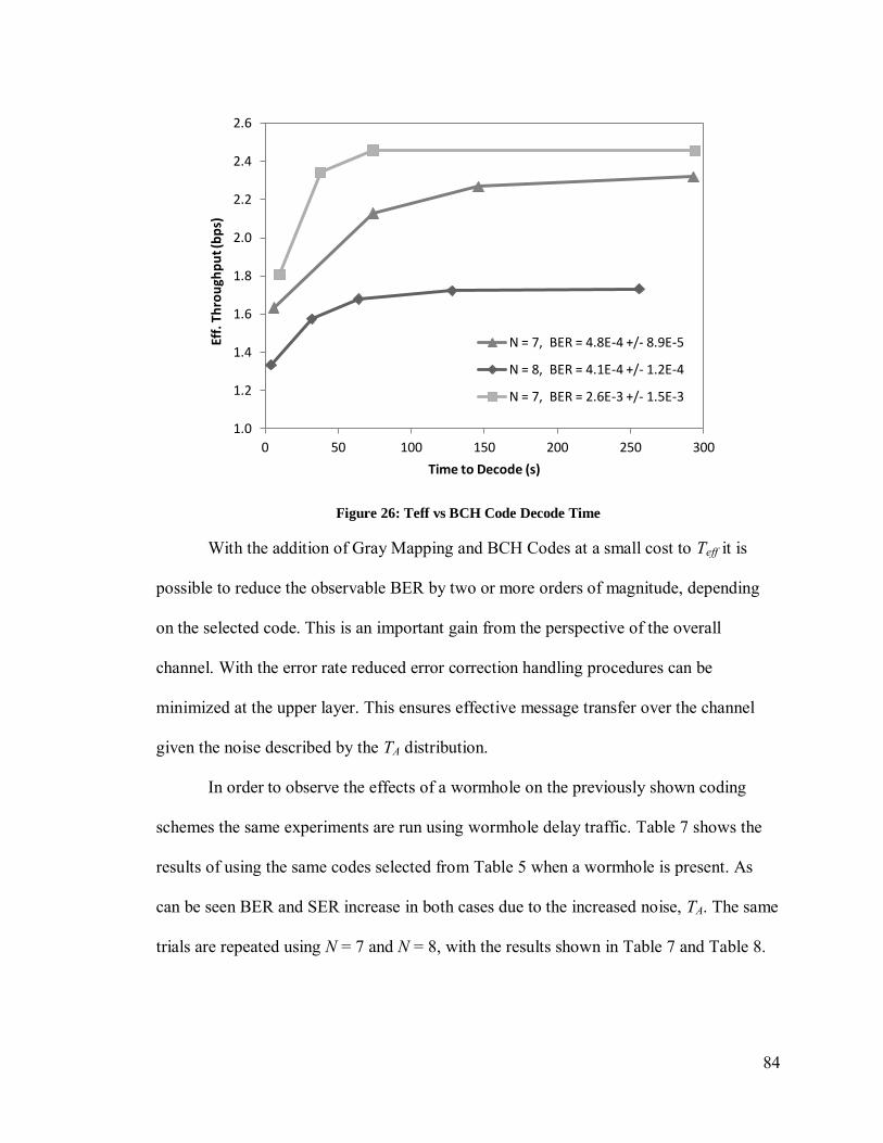
Figure 26: Teff vs BCH Code Decode Time .................................................................. 84 Figure 27: Covert Jitter Distribution .............................................................................. 90
Figure 28: Discrete Keyed Jitter Example ...................................................................... 92 Figure 29: Discrete Jitter Values with Noise TA ............................................................. 92
Figure 30: Wormhole Detection Statistics ...................................................................... 96 Figure 31: Non-wormhole Detection Statistics ............................................................... 96
Figure 32: Wormhole Detection Confidence Intervals.................................................... 98 Figure 33: TA Probability Density Function using Exata ............................................... 100
Figure 34: TA Probability Density Function using OLSRd ............................................ 102 Figure 35: TA Probability Density Function using OLSRd in Noiseless Environment ... 103
Figure 36: TA Probability Density Function using Exata and Test-Bed ......................... 104
Page 9
ix
List of Equations
Equation 1: HELLO Message Interval .............................................................................9
Equation 2: TC Message Interval ................................................................................... 10
Equation 3: OLSR Message Interval .............................................................................. 21
Equation 4: HELLO Message Covert Channel Calculation ............................................ 23
Equation 5: TA Calculation with the presence of a wormhole ......................................... 25
Equation 6: Capacity of a Discrete Noiseless Channel ................................................... 27
Equation 7: Modified Discrete Noiseless Channel Capacity ........................................... 27
Equation 8: Channel Quantization ................................................................................. 27
Equation 9: Self Information .......................................................................................... 29
Equation 10: Entropy of a Random Variable .................................................................. 29
Equation 11: Mutual Information of Two Events ........................................................... 30
Equation 12: Average Mutual Information of Two Random Variables ........................... 31
Equation 13: Discrete Capacity over a Noisy Channel ................................................... 31
Equation 14: Semi-Discrete Capacity over a Noisy Channel .......................................... 33
Equation 15: Approximation of Total Probability .......................................................... 34
Equation 16: Continuous Capacity over a Noisy Channel .............................................. 34
Equation 17: SNR of Discrete Channel .......................................................................... 35
Equation 18: Maximum likelihood Symbol Detection .................................................... 35
Equation 19: Maximum Likelihood Sequence Detection ................................................ 36
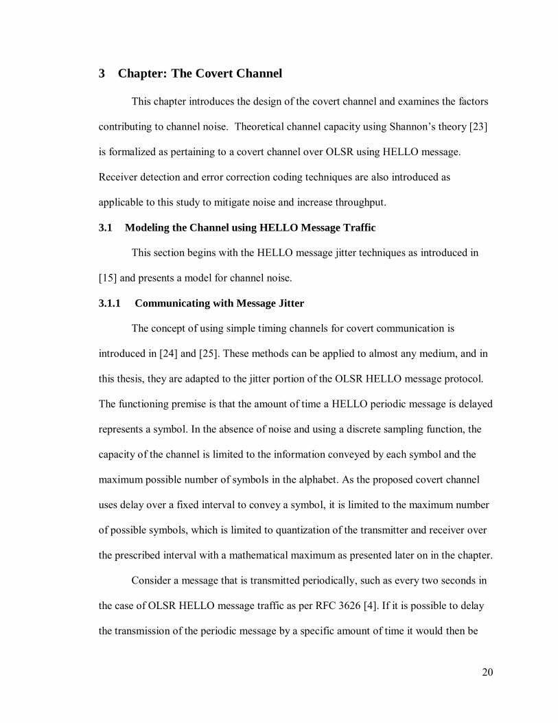
Equation 20: Log-Likelihood Ratio for bit, Bj ................................................................ 39
Equation 21: Log-Likelihood Ratio for bit, Bj of the Covert Channel ............................. 39
Equation 22: Bit Log-Likelihood Example B1 ................................................................ 40
Equation 23: Bit Log-Likelihood Example B2 ................................................................ 40
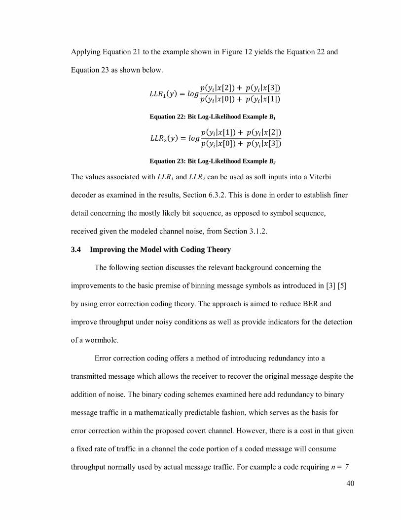
Equation 24: Block Coding Generator Matrix ................................................................ 41
Equation 25: Minimum Hamming Code Distances ........................................................ 42
Equation 26: Kolmogorov-Smirnov Test Notation ......................................................... 48
Equation 27: Throughput ............................................................................................... 76
Equation 28: Effective Throughput ................................................................................ 81
Page 10
1
1 Chapter: Introduction
An ad hoc networking is a network of multiple nodes that operate without
centralized coordination [1]. Nodes can be mobile and join, leave, and re-join the
network. Decisions, such as routing and association, are managed by the nodes
independently. However, increased mobility and decentralized control comes at a cost to
system security in terms of confidentiality, integrity and availability of communications.
Covert communication is defined here as a method of communication where
information passed between entities is undetected and unknown to a third party. Such a
method is invaluable for passing information confidentially. In an environment where
communication is over-the-air and easily visible to multiple parties, applications that are
covert can facilitate secure and reliable communication.
This chapter introduces the motivation, objectives and original contributions of
this thesis. This thesis presents an application of error correction coding theory to a
covert channel in an ad hoc networked environment using the Optimized Link State
Routing (OLSR) protocol. It also presents specific threats, such as “wormhole” replay
attacks, which can be detected using the proposed covert channel coding solution. The
channel is further parameterized in terms of its theoretical capacity and improvements in
reliability over previous models.
Page 11
2
1.1 Motivation
Mobile ad hoc networking applications are well suited for environments that are
highly dynamic, such as mesh networks. Nodes in these networks handle not only their
own traffic but also the traffic of other nodes that use them as intermediary links. This
allows traffic to traverse larger distances, provided a sufficient path of linked nodes
exists. Advantages of MANETs over a centralized control paradigm can be seen from
their inherent redundancy as there is not always a single point of failure in the system.
Ad-hoc networks are able to “self-heal” when a node is removed and do not rely on the
presence of a central entity to maintain their routing configuration for them.
Military applications are well suited to ad hoc networks given that military or
emergency operations require the rapid and mobile deployment of networked assets
where the topology is dynamic. In a multi-group collaborative environment, different
units, often represented by different groups, come together under a unified structure. In
these collaborative group environments the sharing of a common, networked
infrastructure is a basic necessity. In such a scenario it may be required by one sub-group
to identify its specific nodes or pass information in a covert fashion unbeknownst to the
rest of the group. Simply employing encryption between nodes will inform the entire
networked group that private communication is taking place.
Consider a set of networked nodes whose traffic is visible by an external observer.
When an event takes place the observer is able to observe the details of the event by
observing the contents of the traffic passed between nodes. With encryption,
confidentiality of the traffic is ensured as the observer can no longer observe the details
of the event, but by simply observing the encrypted traffic the observer can infer the
Page 12
3
occurrence of an event. With covert communication between the nodes the observer can
neither observe the details of the event nor infer its existence. Also, by effectively
utilizing such a mechanism, it can be ensured that other potential adversaries are not
using the covert channel on the same nodes.
Covert communication could become an avenue for authentication of specific
nodes operating within a shared network. By covertly communicating specific
credentials, nodes could identify each other or act differently towards authenticated nodes
than towards non-authenticated nodes without presenting an easily visible bias. Similarly,
private key distribution over such a scheme along with emergency covert broadcast
traffic alerting only a subset of nodes becomes possible.
Another major security challenge faced by mobile ad hoc networks is the
wormhole attack. Introduced in [2], wormholes have the potential to disrupt or degrade
the efficiency of the network by replaying traffic between nodes in an effort to subvert
traffic and distort nodes’ routing tables. Multiple solutions have been proposed, some of
which are examined in this thesis. This thesis proposes new mechanisms to detect the
presence of wormholes on ad hoc nodes through a natural application of the covert
channel. A node that identifies a wormhole can then adjust its routing tables to ensure
traffic is not hijacked and that traffic proceeds to the next legitimate node whereby
similar mechanisms can provide the same effect and so on as a means to ensure high
availability in a potentially unfriendly environment.
Page 13
4
1.2 Objective
This thesis builds on previous methods of wormhole detection [3] and presents a
mechanism aimed at improving covert channel communication between ad hoc nodes
within the confines of the OLSR routing protocol as defined in RFC 3626 [4]. The
objective is to maximize covert channel communication throughput, minimize error rates
and improve wormhole detection in the network. The seemingly distinct goals of
improving error rates and detecting wormholes are accomplished simultaneously by
applying error correction codes to a covert channel and comparing the bit error rates
against statistical expectations in various levels of noise, where increased noise (and
hence an increased bit error rate) suggests a wormhole may be present.
The central idea of the covert channel is to use a fundamental aspect of the OLSR
protocol HELLO message traffic, known as message jitter. Jitter is a small random delay
generated by each ad hoc node that is normally used to ensure multiple nodes do not
transmit their message traffic at the same time during the broadcast of neighbor discovery
information in the form of HELLO messages. Instead of simply generating a random
jitter delay, this thesis expands the concept, originally discussed in [3] [5], of keying the
jitter with a cryptographic function to pass a covert message, via “random-like” jitter
delay timings defined herein as “keyed jitter”. Given that in a real system there will be an
element of noise still inherent in the covert channel (i.e., uncontrolled delays in
messaging) this thesis examines methods of receiver detection and error correction
coding to reduce the effects of noise and simultaneously provides a metric to detect
network attacks.
Page 14
5
1.3 Outline
In [3] and [5], a method for covert communication that uses timing characteristics
of the OLSR protocol was suggested as a potential future area of study. The proposals
from [3][5] are extended towards a more robust paradigm using coding theory in addition
to addressing concepts of security.
This thesis begins with a relevant description of the technical background of ad
hoc networks and current threats in Chapter 2, as well as assumptions made in this thesis.
Chapter 3 introduces the operating premise of the covert channel using the OLSR
protocol with emphasis on the relevant aspects to this study and without any required
changes to the OLSR protocol. Theory concerning channel capacity is applied and
discussed in the context of the OLSR covert timing channel. The improvements in
channel throughput and reliability from the use of error correction coding and receiver
detection theory are examined against measured SNR and evaluated against the
theoretical maximum of capacity as determined by Shannon’s equations, for point to
point connections.
Chapter 4 presents a criterion for evaluating how difficult it is to detect the
presence of the covert channel. It also considers similar covert channel methods and
possible advantages of using error correctional coding to detect the presence of wormhole
traffic.
Chapter 5 discusses the testing and evaluation aspects of this study in terms of
configuration and setup for simulation, emulation and test-bed scenarios.
The results, presented in Chapter 6, demonstrate the ability to reduce covert
channel error rates through the adoption of coding theory to the proposed channel.
Page 15
6
Different coding methods are compared in terms of their effects on channel throughput
and reliability as well as their ability to be used for wormhole detection.
Chapter 7 concludes with the important highlights of the study reiterating the
contributions presented here.
1.4 Contributions
The following are the contributions of this thesis in bulleted form for clarity and
distinction:
1. This thesis derives the capacity of the covert channel, from [3] [5], and proves
that covert channel capacity can be used to quantitatively detect the presence of a
network attack via a wormhole.
2. It introduces techniques to enhance the reliability (i.e., reduce the bit error rate) of
the covert channel and demonstrate the effectiveness of these techniques, through
extensive simulation, while providing guidance on how to maximize the
throughput with tradeoffs towards the reliability of the channel.
3. It examines methods of ensuring high assurance covert communications and
evaluates the degree to which the proposed timing channel is truly “covert”.
4. Finally, it shows quantitatively, through simulation, that it is possible to improve
network attack detection by observing the performance of the error control codes
derived from the techniques employed in this thesis. It is shown that the number
of errors corrected by the receiver represents a reliable metric for determining the
presence of a wormhole.
Page 16
7
2 Chapter: Background
This chapter presents the relevant background in mobile ad hoc networking as
well as current and prominent threats in mobile ad hoc networking.
2.1 Mobile Ad hoc Networking
Ad hoc networking represents an adaptive solution to a mobile environment
where nodes in the network are neither fixed in time nor place. The two most distinctive
attributes of an ad hoc network are multi-hop relaying and decentralized control. Multi-
hop relaying requires that each node in the network can act as a potential pathway
between two or more other communicating nodes that are out of range of each other.
Decentralized control means that ad hoc networks function without the requirement for
centralized coordination and operate in a distributed fashion whereby each node acts
independently. This allows for a more robust and fault tolerant design, but comes with
additional overhead as each node must maintain network topology and routing
information.
As the topology of all nodes is ever changing, ad hoc routing protocols, are
employed to provide a map from one point to another in the network. These protocols
must continuously update their routes, either reactively or proactively, as discussed in
Section 2.2. The operation of ad hoc networks, including the routing protocols, has been
formalized by a working group within Internet Engineering Task Force (IETF) known as
the MANET Working Group as presented in [6].
Typical environments where mobile ad hoc networks offer advantages are in
environments that require dynamic, scalable and mobile infrastructure. This is true
particularly within the military domain, or organizations involved in emergency
Page 17
8
operations using sensor networks. The next section discusses the types of routing
protocols that operate in these environments.
2.2 Ad Hoc Protocols and Optimized Link State Routing
Ad hoc network protocols can be organized by their route update mechanism,
which is either considered to be table-driven (proactive) or on-demand (reactive).
Nodes using reactive routing schemes, such as Ad Hoc On-demand Distance
Vector (AODV) routing as defined in IETF RFC 35611, determine the route from source
to destination on an as-required basis. Another implementation of covert channels over ad
hoc networking exists in [7][8] using the AODV protocol and is contrasted to this study
in Section 4.5.
Nodes using proactive protocols, which include OLSR, keep network topology
and route information in table format. Generally, the table includes the next node to take
in a path to a particular destination and the expected distance between them. In order to
maintain an accurate picture of the network topology, nodes must exchange routing
update information at the cost of additional overhead traffic compared to reactive
protocols. The advantage being that at transmission time the node can simply send a
packet as opposed to having to seek out routing information. Both proactive and reactive
routing protocols both offer unique advantages to the particular environment for which
they are best suited.
OLSR extends the methodology of proactive routing protocols by offering a
mitigation against the aforementioned route table update overhead by selecting specific
nodes, known as multipoint relays (MPRs), to handle packet forwarding and link state
1 C. Perkins, E. Belding-Royer, and S. Das, “Ad hoc on demand distance vector (AODV) routing,” RFC
3561, July 2003.
Page 18
9
update forwarding. By having fewer nodes responsible for this task, less data
transmission overhead is consumed, resulting in a savings for larger node densities [6].
The OLSR protocol operates by transmitting packets using the user datagram protocol
(UDP). Two message types are involved in passing route information in OLSR: the
HELLO message and the Topology Control (TC) message. The purpose of HELLO
message traffic is to relay neighbor state information, including: link state information
and a list of neighbors that have communicated with the node in the past.
HELLO messages can be sent in a jitter-periodic or HELLO-periodic fashion as
defined in [4] using Equation 1. Jitter-periodic implementations of OLSR define HELLO
message intervals based on when the last message was sent, including its jitter offset.
HELLO-periodic defines the intervals, using Equation 1, but is based on the fixed
HELLO_INTERVAL where jitter is subtracted each time. This thesis uses the HELLO-
periodic approach.
Equation 1: HELLO Message Interval
The HELLO_INTERVAL is periodic every two seconds. The value of jitter from
Equation 1 varies with each successive calculation of the Hello Message Interval with a
range from [0, MAXJITTER], where MAXJITTER is HELLO_INTERVAL/4 or 0.5
seconds as HELLO_INTERVAL is 2 seconds as per [4]. Its intended purpose is to ensure
that if multiple nodes are transmitting, the transmit times are randomized in order to
prevent collisions from nodes transmitting at the same time. This is accomplished by
subtracting a small known random delay, known as jitter, from the HELLO_INTERVAL.
The second type of message worth consideration is the TC message. Its purpose is
to relay topology information used to build routing tables. As per [4] the TC interval is
Page 19
10
defined by Equation 2 . The TC_INTERVAL is five seconds with an additional known
jitter delay of the same range as the HELLO message case.
Equation 2: TC Message Interval
Adjacent nodes which receive HELLO and TC Messages will process them, but
only nodes selected as MPRs will forward them. For the purposes of covert channel
communication the jitter values in both messages can be manipulated to pass a message
undetected, but HELLO message traffic is better suited to this purpose due to its smaller
interval time, thus offering a higher capacity. As well, since the HELLO message is never
forwarded compared to the TC message, there is less confusion around accounting for
multi-hop delays [3].
2.3 Timing Delay Communication with Jitter
Given the brief introduction on the purpose of HELLO message jitter, this section
offers a brief background on how such jitter can be used to convey a covert message. As
introduced in [3] [5] it is possible to introduce deliberate delays (as opposed to random
jitter) on the arrivals of HELLO message traffic between adjacent nodes to convey
information. This is known as a covert timing channel, where information symbols are
represented by the time delay between successive legitimate traffic messages. For
example if a HELLO message arrives at (HELLO_INTERVAL – 0.1s) this represents the
letter “A” and if it arrives at (HELLO_INTERVAL – 0.15s) it represents “B” and so on.
This thesis is concerned with binary communication so the symbols represent binary data,
thus the channel must be quantized into 2N possible values where N is a positive integer.
In order for the receiver to determine which symbol was sent the process of “binning” is
used as illustrated in Figure 1.
Page 20
11
K 2K nK0
...
00 01
t1 t2 tn = Kt0 = (K-K/4)
...
H
10
time
K – K/4 2K – K/4 nK – K/4
jitter
time
Figure 1: Simple Binning
As illustrated in Figure 1 the x-axis shows the time at which a standard HELLO
message, H, is received between the expected minimum and maximum HELLO message
interval values, from Equation 1. For example, in the “zoomed-in” portion of Figure 1, as
the HELLO message, H, is received closer to the symbol value 01 at t1, it can be inferred
that the covert message 01 was most likely sent. The covert message symbols are mapped
to timing delay values of t and defined based on the channel quantization. As the amount
of channel quantization increases, more information can be sent over the channel per
HELLO message interval; however the channel is also more susceptible to errors in this
case. These concepts are further explored in Chapter 3.
Page 21
12
2.4 Medium Access Control with IEEE 802.11
As this thesis is concerned with encoding information in observed message delay,
an understanding of the underlying link layer responsible for message passing is required
as pertaining to the Medium Access Control (MAC) sub-layer defined by IEEE 802.11
[9].
Multiple different types of MAC protocols exist or have been proposed for ad hoc
networking, with 802.11 being one of the most prominent adopted standards. The larger
market share of 802.11 devices offers greater relevance to this study as well as a larger
comparative base of literature from which to evaluate the results of a covert channel over
802.11.
802.11 MAC uses Carrier Sense Multiple Access with Collision Avoidance
(CSMA/CA) in order to determine when a node should transmit on the shared channel. If
a node wants to send data, it first listens to the channel and starts sending a frame if the
channel is not busy. Should the channel be busy, the sender waits a random transmitter
assigned contention back-off period defined as a random multiple of 20µs slot sizes after
which re-transmission is attempted.
802.11 MAC operates, generally, in either one of two modes: either a distributed
coordination function (DCF) mode or a point coordination function (PCF) mode. The
difference between a PCF and DCF is the absence of a centralized coordinator in a DCF.
A PCF system usually applies to current home 802.11 wireless access using an Access
Point as a PCF to coordinate traffic amongst nodes. A DCF system usually uses
CSMA/CA to determine when to send messages in the absence of a PCF. Messages that
are transmitted must also adhere to specific Inter Frame Spacing (IFS) requirements.
Page 22
13
Control messages can wait either short-IFS (SIFS), or a DCF-IFS (DIFS) with delays that
vary with priority or depending upon physical layer characteristics, such as the choice of
modulation. The reader is encouraged to examine the 802.11 IEEE standards [9] for more
detail.
A DCF is the mode modeled in this thesis in regards to the simulation, emulation
and test-bed scenarios. Under high traffic environments, the delay experienced by a node
waiting to send a message is expected to become larger due to collisions and back off.
Constant collisions between nodes transmitting HELLO message traffic results in a more
unpredictable HELLO message interval. Since the approach in this thesis uses the
HELLO message timing as a means of covert communication, as explained briefly in
Section 2.3 and further detailed in Chapter 3, any increased variation in HELLO message
arrival leads to channel noise and could contribute to an increased Bit Error Rate (BER)
of the covert channel studied in this thesis.
Propagation delay between nodes is significantly smaller (i.e 300ns for a 100m
link) than delays caused by collision and back off, and is considered negligible for this
thesis. A fully documented study of HELLO message propagation delays is presented in
[3]. This thesis will attempt to quantify these delays under specific conditions and will
use error correction coding decisions to improve HELLO message covert channels
mentioned in [3] [5].
Page 23
14
2.5 Security Challenges to MANETs
This section briefly introduces the prominent threats inherent in mobile ad hoc
networking which can vastly affect performance or represent security risks.
2.5.1 Wormholes
The wormhole attack, as applied to ad hoc networks, is first introduced in [2] and
described using Figure 2.
21
Figure 2: Nodal Representation of a Wormhole
In this figure the light colored nodes represent legitimate nodes. In the functioning
of normal OLSR protocol operations these light colored nodes would transmit HELLO
messages allowing the nodes to identify their neighbors and generate applicable routing
table and topology information. Should Node 1 need to send traffic to Node 2 a potential
path is identified, shown using the connected lines between the light colored nodes in
Figure 2, consisting of multiple hops through the network.
With the introduction of a wormhole, depicted by the black nodes, it becomes
possible to disrupt the topology. These nodes do not act as members of the topology and
therefore do not transmit legitimate message traffic or appear as members of the network,
but rather passively receive and forward all traffic, known as tunneling. This is explicitly
accomplished by the wormhole nodes transmitting between each other on an off-channel
Page 24
15
link and then re-broadcasting. The effect is that instead of the path depicted in Figure 2, it
will appear that Node 1 and Node 2 are next to each other and their routing topologies
will be updated as such. As all the nodes on the left and right side of the diagram, by the
means of the wormhole, appear right next to each other.They will fail to seek new routing
information and will transmit all traffic through the wormhole.
There are multiple consequences of wormhole manipulation. First, as traffic is
now routed through the wormhole, the topology is lost, as inspection of the routing tables
demonstrates that distant nodes are in proximity of each other. The wormhole channel
can now function as a Man-In-The-Middle (MITM) attack and alter traffic at will,
opening up a host of malicious possibilities. Once the wormhole channel is removed all
routing topology needs to be reset causing a temporary denial of service.
As proposed in [2] one defense against wormholes uses the concept of “Packet
leashing” whereby the node’s known location is used to predict wormhole presence.
Another method uses direction finding equipment to predict wormholes, as in [10]. Other
approaches exist around modification to the OLSR protocol, as discussed in [11], through
the addition of modified HELLO message types targeted at using a timing analysis of
HELLO message packet delivery. New algorithms are also proposed in [12] [13] [14]
offering unique and effective approaches to wormhole detection at the expense of
changes to the underlying OLSR protocol or additional constraints on neighboring nodes
in terms of synchronization.
The approach taken in this thesis, through the use of the covert channel, differs
from the aforementioned approaches in that it retains compatibility with the original
OLSR protocol and does not require any changes to message type or overarching
Page 25
16
protocol structure. The work discussed extends that of [15] [16] using packet timing
statistics, bit error rate (BER) and tracking corrected errors from channel encoding as
additional predictors of wormhole attack in a system of nodes. All the processing
required to detect wormhole channels can be implemented within the node internally
without changes to the functionality of the protocol, thus maintaining compatibility with
unmodified nodes.
2.5.2 Trust in Sensor Networks
Trust plays an important role in any ad hoc network, where any node can join or
act as a message forwarding intermediary. In a secure environment, it becomes
particularly important to ensure the integrity and authenticity of nodes operating in an ad
hoc environment. The OLSR protocol is defined on principles based on a complete trust
of neighboring nodes without applicable security controls inherent in its design. In one
sense this makes the protocol simple to implement and allows for interoperability
between nodes using open standards, yet adds a degree of risk from a security perspective
as this exposes the network to potential attack.
As discussed in [17], there exist multiple vectors of attack in ad hoc networks.
Network attacks through wormholes as previously discussed are possible. Should the
wormhole decide to drop all packet traffic it then becomes a so called “Black hole”.
Attacks where malicious nodes are introduced to the network are possible as well.
Specific attacks include the fabrication of false routing information used to disrupt the
topology and routing tables of cooperative nodes, along with impersonation of nodes
acting on behalf of legitimate nodes for nefarious purposes.
Page 26
17
Traditional approaches towards the active attacks utilize principles of
cryptography [17] to build trust models between nodes, but this is done at either a cost to
overall capacity or additional changes to the OLSR protocol [18] [19], among others. The
goal of this thesis is to maintain interoperability with partner organizations or cooperative
environments sharing nodes in a network where it may not be possible to share security
details. The covert channel proposed in this thesis offers a potential mechanism of
allowing for authentication of nodes and mitigation of fabricated or “replay attacks” from
suspicious nodes through its use.
Trusted nodes can authenticate each other through covert traffic while
maintaining interoperability with existing nodes on the network. Depending on the
topology, decisions can be taken by each node to use routes through trusted nodes
(instead of potentially faster routes) or over un-trusted nodes in specific situations. This is
depicted in Figure 3 where the light colored nodes represent trusted nodes authenticated
through covert messages. In this example, a routing path is present between only trusted
nodes connected by solid lines, which can be used to ensure trusted message delivery.
Interoperability between light and dark colored nodes exists, but can be elected to be
handled differently by the trusted nodes as required without impact to the basic operating
principals of the OLSR protocol. It is noted that keyed jitter can only maintain the
authenticity of HELLO messages as used to identify friendly nodes and pass covert
messages between them, and not the authenticity of non-covert transmitted traffic, which
is still subject to over-the-air attack. Additionally, should replayed or fabricated traffic
contain HELLO messages without appropriately keyed jitter, this can serve as a signature
for potentially malicious traffic.
Page 27
18
Figure 3: Trusted Node Routing
A particular application of a covert channel may exist in authentication in sensor
MANETs where large sets of nodes are deployed. Authentication over a covert channel
could offer a means to establish trust throughout the network. This approach guards
against false sensors potentially placed in the network to obscure data retrieval or disrupt
functionality.
2.6 Assumptions and Limitations
In order to focus on specific aspects of covert message traffic over the OLSR
protocol it becomes necessary to make reasonable assumptions of the underlying traffic
channels and hardware.
As discussed in further detail in Chapter 3, cryptographically keyed jitter is added
to HELLO messages when creating the covert channel. These cryptographic
pseudorandom generators are utilized in order to preserve the inherent randomness of the
OLSR jitter. Also, it is assumed that cryptographic key distribution between nodes is
completed without risk of access by a malicious third party. The study of the
effectiveness of the different options available for various levels of cryptographic
strength is beyond the scope of this thesis with the assumption that the cryptographic
Page 28
19
portion of this thesis is a “pluggable ” aspect of design with the degree of cryptographic
security required to meet the application.
The nodes communicating covertly are considered to be friendly and not
compromised. Only attacks against the OLSR routing scheme, via wormholes, or
eavesdropping are considered. Wormholes are modeled as being passive in the sense they
are not actively dropping packets. Systems of re-syncing cryptographically keyed traffic
between nodes exist [20][21][22], but are outside of the scope of this thesis. It is assumed
that if a HELLO packet is dropped the receiver simply advances the keyed jitter stream
by one position2.
In order to gauge the effectiveness of the error correction coding schemes utilized
within this thesis, it is best to contrast the results to theoretical expected maxima. The
limiting factor of timing-delay manipulated covert message traffic between nodes is the
sensitivity of the transmitting and receiving nodes signal sampling hardware. Thus, it is
assumed that the smallest unit of measurement possible, by receiving hardware as
required by the OLSR protocol, is the minimum back-off interval slot time of 20µs as
specified in IEEE 802.11 [9]. As some of the tools used in this thesis are able to measure
units as small as 1µs this is also considered exceeding the bounds of the IEEE standard.
2 A wormhole is free to manipulate all traffic including HELLO message traffic, but to drop HELLO
packets is ineffective as this defeats the effect of the wormhole. The methods considered in this thesis
examine HELLO message delays and are independent of HELLO message content.
Page 29
20
3 Chapter: The Covert Channel
This chapter introduces the design of the covert channel and examines the factors
contributing to channel noise. Theoretical channel capacity using Shannon’s theory [23]
is formalized as pertaining to a covert channel over OLSR using HELLO message.
Receiver detection and error correction coding techniques are also introduced as
applicable to this study to mitigate noise and increase throughput.
3.1 Modeling the Channel using HELLO Message Traffic
This section begins with the HELLO message jitter techniques as introduced in
[15] and presents a model for channel noise.
3.1.1 Communicating with Message Jitter
The concept of using simple timing channels for covert communication is
introduced in [24] and [25]. These methods can be applied to almost any medium, and in
this thesis, they are adapted to the jitter portion of the OLSR HELLO message protocol.
The functioning premise is that the amount of time a HELLO periodic message is delayed
represents a symbol. In the absence of noise and using a discrete sampling function, the
capacity of the channel is limited to the information conveyed by each symbol and the
maximum possible number of symbols in the alphabet. As the proposed covert channel
uses delay over a fixed interval to convey a symbol, it is limited to the maximum number
of possible symbols, which is limited to quantization of the transmitter and receiver over
the prescribed interval with a mathematical maximum as presented later on in the chapter.
Consider a message that is transmitted periodically, such as every two seconds in
the case of OLSR HELLO message traffic as per RFC 3626 [4]. If it is possible to delay
the transmission of the periodic message by a specific amount of time it would then be
Page 30
21
possible for the receiver to distinguish this delay as a symbol, independent of the actual
message sent, which is the basic tenant of the simple timing channel as proposed by [25].
In order to be truly covert the action of delaying transmission of a message must
be consistent with the terms of the underlying protocol so as not to arouse “statistical
suspicion”. In the case of OLSR the application of covert messages is realizable, as
demonstrated in [15], through the express terms of the protocol itself. In order to ensure
multiple nodes do not transmit their HELLO messages at the same time a random jitter
value is subtracted from the HELLO_INTERVAL of two seconds as per [4], shown in
Equation 3. The ith
actual HELLO interval is defined by subtracting the ith
random jitter
value from a fixed HELLO_INTERVAL from.
Equation 3: OLSR Message Interval
The jitter is limited to a randomly selected value between 0 and
, as per [4], where K is
the HELLO message interval of two seconds.
The approach taken in this thesis is to substitute the randomly selected jitter value
with a message value that is obscured by a cryptographically strong pseudo random
number generator given some shared secret seed value, for the purpose of conveying a
covert message. This allows the sender to manipulate a hidden message with a
cryptographically generated key value; this hidden message is sent as the jitter, jitter[i],
in Equation 3. At the receiver it is then possible to generate the same cryptographic key
stream, using pre-shared keys, and remove this value from the expected HELLO interval
to regain the hidden message contained in the remaining deliberate jitter value. This is
demonstrated in Figure 4 where the message, conveyed using deliberate jitter, TDJ[i], is
Page 31
22
manipulated with a key value, TKJ[i], shared between sender and receiver. At the receiver
side TKJ[i] is removed resulting in the original message conveyed with TDJ[i].
Sender
TDJ[i]
TKJ[i]
TKJ[i]
TKJ[i]
Receiver
TDJ[i]
Channel
TDJ[i]
Figure 4: Covert Channel Mechanism
Covertness of the channel is maintained as the purpose of jitter induced delay is
already an integral part of the protocol and therefore does not break any expected
operating norms. A more thorough discussion of stealth is presented later in Section 4.1.
The conceptual model presented above is lacking with respect to the addition of
noise introduced through additional delay factors that need to be considered in real world
systems. In any system using a protocol stack, as implemented in this thesis, there will
exist delays inherent in protocol stack traversal, such as CPU and operating system
overhead to name a few. An analysis of all the specific delays inherent in an OLSR
system has already been conducted in [3]. In this thesis all delays are amalgamated into
one variable, TA, representing all unknown random jitter present in the system. Mitigating
the effects of the variable TA, on the proposed covert channel, through the use of error
correction coding theory will be the focus of this thesis and central to the results in
Chapter 6.
Page 32
23
To better understand how TA affects the covert channel consider the following
model in Equation 4 where ∆t represents the time between successive HELLO messages
as measured by the receiver. THP is the HELLO_INTERVAL, or two seconds, as per the
OLSR protocol. TDJ[i] is the ith
deliberate jitter XORed with the ith
keyed jitter, TKJ[i],
used to encrypt TDJ[i] and ensure jitter values are uniformly distributed. The remaining
uncontrolled element is TA[i] representing the unknown jitter random variable caused by
message handling overhead between successive sender delay, denoted as TSD[i], and
receiver delay, denoted as TRD[i] as shown in Equation 4.. For a detailed breakdown of all
the contributing factors associated with these delays the reader is directed to [3].
Equation 4: HELLO Message Covert Channel Calculation
After measuring ∆t and removing the known value of THP the remaining result of
is passed to the receiver which estimates
then removes TKJ[i] to recover the original message, TDJ[i]. In reference with [3] this is
known as HELLO-periodic HELLO message timing.
At this point, it is possible to demonstrate the effects of TA on the covert channel
implementation using HELLO message jitter delay show in Figure 5.
Page 33
24
00 01
t1 t2 tnt0
...
TDJ
10
time
TDJ + TA
Figure 5: Simple Binning with Delay Added
In this example the intended covert symbol, TDJ = 01, is delayed between the
sender and receiver by TA. This causes the received symbol to appear closer to the value
10. The receiver could then incorrectly decode the symbol to be 10 when 01 was the
transmitted symbol. Techniques introduced in this thesis are designed to mitigate the
errors from delay introduced by TA.
3.1.2 Receiver Noise and Delay
An alternative way to represent TA is shown by the sequence diagram in Figure 6
where the elements of Equation 4 are shown with the unknown delays shown by the
darker boxes. Should all delays on both the sender and receiver be fixed constants TA
would reduce to zero, but due to the complexities of stack propagation, CPU overhead
and other priority schemes within computing hardware these delays will vary. A more
detailed discussion of all the potential delays inherent in a system has already been
produced in [3] and is therefore only summarized here as pertaining to the determination
of TA. Should a wormhole be present an additional variable is introduced, TWD,
representing the additional delay added from the wormhole.
Page 34
25
Sender Receiver
HELLO Message
∆ t HELLO Message
time
(TKJ TDJ)THP –
Figure 6: HELLO Message Sequence Chart
The addition of the wormhole results in a sequence diagram as shown in Figure 7
(next page) with the black delay boxes. For the purposes of this thesis the additional
delay caused by a wormhole has already been demonstrated in [5] [16] as a random
variable with an associated Rayleigh probability distribution (σ=0.002s). Therefore in the
presence of a wormhole the value of TA[i] is shown in Equation 5. It has been shown
previously in [3] that the difference in statistical properties of TA between samples
recorded with and without the presence of a wormhole can be used as a means to detect a
wormhole attack. This thesis focuses on this concept.
Equation 5: TA Calculation with the presence of a wormhole
Page 35
26
Sender WormHole
HELLO Message
HELLO Message
Receiver
HELLO Message
HELLO Message ∆t
time
(TKJ TDJ)THP –
Figure 7: Wormhole Message Sequence Chart
3.2 Calculating Channel Capacity
In order to better understand the practical limitations of a covert channel
mechanism over OLSR an understanding of the channel capacity is required. The
following sections serve to offer background pertaining to theoretical channel capacity in
both the noiseless and noisy channel cases. The theoretical background will be utilized in
the results section as a guide to the overall effectiveness of any suggested coding schemes
or measures aimed at reducing channel BER.
3.2.1 Capacity of a Noiseless Channel
HELLO message timing intervals are defined within [4] to be limited to a period
of two seconds, defined by K, with an accepted jitter limited to a uniform distribution
with a maximum range of [0, K/4] per each HELLO message interval. It has been
previously proposed that a covert channel can be created by modulating HELLO message
traffic between a sending and receiving node [5, 15]. The overall capacity, C, of a
Page 36
27
noiseless discrete point to point timing channel is given by [23] and modified by [25] as
written in Equation 6.
Equation 6: Capacity of a Discrete Noiseless Channel
Here N(t) defines the number of unique symbols that can be represented over an
interval of time t. As the HELLO message period, t, is limited by K, the HELLO message
interval, the model for noiseless capacity can be modified to Equation 7 as discussed in
[26] where M is the total number of symbols. Symbols are defined using a specific
interval, or bin, limited to the minimum channel quantization TQ achievable by the
receiving node. This is limited by the maximum allowed jitter range of [0,K/4], and
symbol count, M with N bits per symbol, shown in Equation 8.
Equation 7: Modified Discrete Noiseless Channel Capacity
Equation 8: Channel Quantization
Equation 7 shows that the receiving node quantization must double for each additional bit
in channel capacity C per period K. In practical terms the limiting factor may be the
capabilities of the hardware in the noiseless case.
A current hardware limitation for quantization, TQ, can be approximated by the
IEEE 802.11 standard’s [9] smallest resolvable time slot, the back-off interval slot time,
which is 20µs. Using Equation 8 this gives M = 25000 possible symbols which
Page 37
28
approximates to a 14.6 bit capacity per period, K, or 7.3 bps under noiseless conditions
as a current theoretical maximum assuming discrete time intervals and no channel noise.
3.2.2 Deriving the Capacity of a Noisy Channel.
As a noiseless communication channel between nodes represents an unrealistic
assumption towards communication, a more accurate upper bound of expected capacity is
sought. Guidance is derived from the previous methods proposed by C.E. Shannon’s:
Theory of Communication [27]. The broad concepts discussed in this section include:
Self-Information, Entropy and Mutual Information which are used in Shannon’s
equations to compute channel capacity for a noisy channel. Here these concepts are
applied to find the capacity of the HELLO message timing delay based covert channel.
3.2.3 Self Information
Self information relates to a measure of information about the outcome of events
with a defined set of probabilities. Consider a random variable X, which can take on a
number of values. When a particular occurrence of X = x[j] is observed this relates to a
measureable unit of Self Information of that specific occurrence satisfying three
properties:
1. The probability of an event is inversely proportional to the amount of
information received from its occurrence.
2. An event that occurs with ultimate certainty gives no information.
3. If the observance of x[j] can be represented by two successive and
independent, or mutually exclusive events, then the information rendered
is equivalent to the sum of information from observing both events
independently.
Page 38
29
The above series of properties can all be satisfied by Equation 9 where P(x[j]) represents
the probability of the occurrence of the event x[j].
Equation 9: Self Information
The logarithmic base of Equation 9 is chosen to be two, so as to measure information in
units of bits, consistent with the previous section, and is a measure of the information
associated with the observance of a particular event.
A sample application of this equation is illustrated by observing the amount of
information conveyed by the outcome of the toss of a two sided coin toss where each face
of the coin occurs with probability of one-half. This will convey log2(2) or one bit of
information, either on the observance of a “heads” or “tails” assuming the probability of
each event is equal.
3.2.4 Entropy
While Equation 9 gives a defined amount of information from a specific
occurrence of the event x[j] the average self information of a random variable is called
the entropy. The following formula provides a definition of the entropy associated with
the random variable X which is consistent with the properties of self information and
measured in bits.
Equation 10: Entropy of a Random Variable
Applying this to the example using a two sided coin gives H(X) = 1 bit of entropy for a
single coin toss.
Page 39
30
3.2.5 Mutual Information
Adding further to the previous section, consider two random variables whereby
the output of X is denoted by x[j] ∣ j ∈ℤ+ and the outcome of Y is denoted by y[k] ∣ k
∈ℤ+. Consider the case where the event y[k] is observed. In order to establish how much
information the observation of y[k] conveys about the occurrence of the event x[j] a
definition of mutual information is required. Staying consistent with the properties of self
information the following properties are required for mutual information:
1. If the random variables X and Y are independent their observance of y[k]
provides no information about the occurrence of x[j], therefore there is
zero mutual information.
2. If the random variables X and Y are equal then the observance of y[k]
provides all required information about the occurrence of x[j] and would
equate to the measure of self information of x[j] as per Equation 9.
Mutual information is therefore defined in the following equation where is
the mutual information between y[k] and x[j] with as the conditional
probability of y[k] given x[j] has occurred and is the probability of x[j]
and y[k] occurring jointly.
Equation 11: Mutual Information of Two Events
The average mutual information of two random variables is found in Equation 12 by
finding the expectation of Equation 11 over all x[j] and y[k]. A logarithmic scale of base
2 is used to obtain the average mutual information in bits.
Page 40
31
Equation 12: Average Mutual Information of Two Random Variables
3.2.6 Noisy Channel Capacity Calculations
It is now possible to provide a mathematically derived upper bound for the
expected capacity of a channel transmitting in the presence of additive noise. Assume a
system as demonstrated in Figure 8. Here, X represents the signal input random variable
synonymous with TDJ as sent from the transmitter from Section 3.1.1. Y denotes the
output random variable altered as a result of the noisy channel and represents the value of
TDJ + TA as observed by the receiver. Both X and Y are discrete random variables with a
probability that y[k] is received given x[j] was sent of .
Input X Output Y
Figure 8: Communication over a Noisy Channel
Channel capacity, C, is measured in bits per channel use, or period in the case of
HELLO message traffic over OLSR, and represents the theoretical maximum error free
information transfer rate between a transmitting and receiving node. The capacity is
defined then by the maximum mutual information resulting between the input X and
output Y where I(X,Y) is maximized over the set of all possible input probabilities, P(x[j])
as shown in Equation 13.
Equation 13: Discrete Capacity over a Noisy Channel
Noisy Channel
Page 41
32
Capacity then depends on P(y[k] | x[j]). However, as y[k] = x[j] + TA this implies that
P(y[k] | x[j]) depends entirely on the noise statistics of TA. Equation 13 represents the
scenario whereby the transmitter’s input into the channel and the receivers output from
the channel are limited to discrete values. In the context of the proposed covert channel
communication mechanism from Section 3.1.1, the transmitter is limited to a fixed
number of possible symbols which translates into a discrete set of potential delays
between [0,K/4]. is the total probability of Y. Equation 13 is best suited for
application where the sender and receiver use fixed bin sizes, limited by TQ and “hard
decisions”, of being in either one bin another, in regards to y[k]. This is demonstrated in
Figure 9 where y[k] must either be interpreted as x[j+1] or x[j+2] using a hard decision
technique.
00 01
x[j+1] x[j+2] x[j+n]x[j]
...
TDJ
10
time
TDJ + TA
y[k]
Figure 9: Discrete Binning with Delay Added
For the HELLO message jitter manipulated covert message passing, the input X is
limited to a discrete set of values, limited to M slots between 0 and K/4. The output value,
Y, however may not be limited to a set of discrete points. This is demonstrated in Figure
10 similar to Figure 5 where the generic time values, t, are replaced by the transmitter slot
times; x[j]. Here the receiver can determine the exact continuous value for received time,
Page 42
33
TDJ + TA, and does not need to round to the nearest value of x[j+2] as in the discrete-
discrete case from Equation 13.
00 01
x[j+1] x[j+2] x[j+n]x[j]
...
TDJ
10
time
TDJ + TA
y[k]
Figure 10: Semi Discrete Binning with Delay Added
Should Y be continuous with a discrete input value X it is shown that Equation 13
changes to the semi-discrete case where Equation 13 is modified to produce Equation 14.
Here the receiver can record the exact value associated with the observed value of y[k].
Being able to record the added information associated with difference between y[k] and
x[j+1], using Figure 10 as an example, allows for the use of “soft decision” methods that
can evaluate probabilities with more precision based on a series of measurements.
becomes the conditional probability density function of Y given x[j] has been
sent. is again the total probability of Y.
Equation 14: Semi-Discrete Capacity over a Noisy Channel
Equation 14 is best suited to determining the upper bounds of the covert channel
with inputs x[j] defined by the channel quantization from Equation 8 as messages are sent
from the transmitter. At the receiver side it is assumed, in accordance with previous
Page 43
34
statements, that the receivers’ quantization is limited to the IEEE 802.11 standard’s [9]
smallest resolvable time slot, the back-off interval slot time, which is 20µs. Equation 14
is then approximated using a transmitted message, x[j], with a slot size of TQ from
Equation 8 and a received message slot size, y[k] of 20µs. This translates to using fixed
sender bin sizes, limited by TQ and soft decisions in regards to y[k]. The total probability,
, is approximated using Equation 15. Additionally, as X is determined to be
uniformly distributed, as per the requirements of the OLSR protocol, will
become a fixed constant equal to
where N is the number of bits used to quantize the
channel.
Equation 15: Approximation of Total Probability
In order to find the highest possible theoretical capacity of the covert channel in
the presence of noise, any limitations of sender and receiver quantization are eliminated.
This is expressed in Equation 16 where is defined by the probability density
function (pdf) of the uniform random variable with
with
and as
the total probability of Y as per Equation 15.
Equation 16: Continuous Capacity over a Noisy Channel
Equation 14 and Equation 16 become useful to gauge the effectiveness of the
chosen encoding schemes used during simulation and experimental results against the
effective channel capacity limitations. They will also offer additional insight into the best
Page 44
35
choice of N (bits per symbol) used by the system given the properties of the measured
noise in the channel.
In Chapter 6 these capacity equations will be evaluated for channel
characterizations obtained through extensive simulation and compared to channel signal
to noise ratio (SNR). Channel SNR is calculated, as adapted from [28] , in the discrete
case, using a ratio of mean signal, which is channel quantization, to the standard
deviation of the noise process, TA, as per Equation 17.
Equation 17: SNR of Discrete Channel
3.3 Receiver Detection Theory
Techniques that may serve to further reduce the bit errors can be applied by the
receiver of a covert message and should be examined first before introducing additional
overhead associated with error correction coding. This section examines these techniques.
3.3.1 Maximum likelihood Symbol Detection
Given the receiver has an understanding of the noise through the distribution of TA
it becomes possible to make decisions based on the probability of a symbol, x[j], being
sent where x[j] denotes a discrete symbol between [0,M). The receiver can estimate the
most likely symbol, x[j] transmitted, given a continuous value, y, is observed at the
receiver. This is formalized in Equation 18 using Bayes’ Rule. That is, the receiver can
estimate the value x[j] that maximizes P(x[j] | y) as expressed in Equation 18.
Equation 18: Maximum likelihood Symbol Detection
Page 45
36
The reduction realized on the right hand side of the equation is possible by assuming
due to the nature of the uniform distribution of symbols. The probability of
y, denoted p(y), is the summation of all probabilities of a particular observed value, y,
given all possible inputted discrete symbols, x[j].
The selection of x[j] is found by choosing the symbol x[j] that maximizes the
value of Equation 18. This is called the maximum likelihood detector. In Section 6.2.1, it
is found that a maximum likelihood symbol detector for the covert channel functions as a
simple minimum distance detector.
3.3.2 Maximum likelihood Sequence Detection
Should the receiver maintain a memory of all received symbols, as implied
through the use of larger codes which are subdivided into particular block sizes for
transmission, it is possible to make statistical predictions from the received sequence
vector, y = (y1 , y2, … yn) observed by the receiver for a given vector of transmitted
symbols x = (x1[j1 ],x2[j2], …xn[jn]). In this case Equation 18 can be represented using
Equation 19.
Equation 19: Maximum Likelihood Sequence Detection
In maximum likelihood sequence detection, then, the receiver chooses the sequence x that
maximizes .
Page 46
37
3.3.3 Gray Mapping
Gray Mapping, originally patented by Frank Gray at Bell Telephone [29], is a
method of mapping bits to symbols so as to ensure the bitwise difference between two
adjacent symbols, or Hamming distance, is one bit. For example, the binary sequence 00,
01, 10, 11 becomes 00, 01, 11, 10 after Gray Mapping. The advantage of this scheme is
that when errors or noise are introduced into a system such that adjacent symbols may be
mistakenly received the resulting bit error is minimized. To best illustrate this observe the
symbol mapping in Figure 11. This depicts M = 27, or 7-bit symbols. The advantage can
be seen when the standard binary coding scheme the binary value 0000111 is transferred
and additional noise, sufficient enough to cause displacement by a half-symbol, will
cause a 4-bit error from the decoded value of 0001000 with a Hamming distance of four.
When Gray Mapping is applied the Hamming distance is reduced to one bit for adjacent
symbols.
0000
100
0000
101
0000
110
0000
111
0001
000
TQ
Sample
Sample +
noise
… K/4
0000
011
0000
010
0000
110
0000
111
0000
101
TQ
Sample
Sample +
noise
… K/4
4 bit error
1 bit error
Gray Mapped Values
Binary Coded Values
Figure 11: Gray Mapping Example
Page 47
38
3.3.4 Symbol Reliability with Bit Log-Likelihoods
The output from a Maximum Likelihood Symbol Detector, as discussed in
Section 3.3.1, is a decision on the most probable symbol received. It is sometimes
desirable, however, for the receiver to further compute the likelihood of receiving each
individual bit in every symbol, as opposed to simply computing the most likely symbol.
This is of particular importance when using a Viterbi decoder for soft decision decoding,
discussed in Section 3.4.3, whereby a specific confidence rating is assigned to each bit
input to the decoder.
The concept of bit-reliability is demonstrated in Figure 12. In this example
Symbol sizes of N = 2 are chosen and ordered using Gray Mapping, from Section 3.3.3,
at widths of TQ from Equation 8. The received delay, y, is shown between two symbols,
x[2] and x[3], respectively. In a “hard decision” decoding scheme y would be interpreted
as its closest neighboring symbol, as x[2]= 11 in this case. When examining the
reliability of the individual bits associated with the received symbol it is possible to
predict the received symbol to a higher degree of precision. Of the two adjacent symbols
to y, being x[2]and x[3], when examining the left most significant bit (MSB) and least
significant bit (LSB) different probabilities arise.
00 01 11 10
x[0] = 0 x[1] = x[2] = x[3] =
y
TQ 2TQ 3TQ
Figure 12: Bit Log-Likelihood Example
Page 48
39
It can be seen that of the adjacent potential symbols the likelihood of the MSB being
interpreted as the value “1” is greater than the LSB being interpreted as the value “1” for
a message received at delay, y. In this scheme the likelihood of the LSB being decoded in
error is greater than the likelihood of the MSB being decoded in error. The only chance
of the MSB being incorrectly interpreted is by a larger error delay from the transmitted
delay.
In order to mathematically quantify this relationship the following notations is
adopted. The bit-wise representation of any symbol becomes B1B2..Bn | Bj (0,1) where Bj
represents each individual bit position in the symbol from MSB to LSB. Given an
observed delay, y, the probability of Bj = “1” or “0” is defined by the likelihood, p(y |
Bj=1) and p(y | Bj=0). Therefore the Log-Likelihood Ratio (LLR) is described using
Equation 20.
Equation 20: Log-Likelihood Ratio for bit, Bj
The value derived from LLRj(yi) represents the reliability of bit Bj. A negative value
indicates a greater reliability towards Bj = 0, while a positive value gives a higher
reliability towards Bj = 1. In order to evaluate Equation 20 the numerator and
denominator must consider all the symbols whereby Bj = 1 and Bj = 0. Using the notation
x1[j] | j … N) to denote all the symbols where Bj = 1 and x0[k] |k (0, … N)
to denote all the symbols where Bj = 0, Equation 20 becomes Equation 21.
Equation 21: Log-Likelihood Ratio for bit, Bj of the Covert Channel
Page 49
40
Applying Equation 21 to the example shown in Figure 12 yields the Equation 22 and
Equation 23 as shown below.
Equation 22: Bit Log-Likelihood Example B1
Equation 23: Bit Log-Likelihood Example B2
The values associated with LLR1 and LLR2 can be used as soft inputs into a Viterbi
decoder as examined in the results, Section 6.3.2. This is done in order to establish finer
detail concerning the mostly likely bit sequence, as opposed to symbol sequence,
received given the modeled channel noise, from Section 3.1.2.
3.4 Improving the Model with Coding Theory
The following section discusses the relevant background concerning the
improvements to the basic premise of binning message symbols as introduced in [3] [5]
by using error correction coding theory. The approach is aimed to reduce BER and
improve throughput under noisy conditions as well as provide indicators for the detection
of a wormhole.
Error correction coding offers a method of introducing redundancy into a
transmitted message which allows the receiver to recover the original message despite the
addition of noise. The binary coding schemes examined here add redundancy to binary
message traffic in a mathematically predictable fashion, which serves as the basis for
error correction within the proposed covert channel. However, there is a cost in that given
a fixed rate of traffic in a channel the code portion of a coded message will consume
throughput normally used by actual message traffic. For example a code requiring n = 7
Page 50
41
bits of coded message with k = 4 actual message bits actually sent. From inspection n – k,
or 3 bits, are consumed by the encoding scheme for a total message information size of k
bits.
3.4.1 Block Coding Schemes
In the linear block coding schemes a k-bit message block is mapped to an n-bit
code block such that n > k. The code rate R, is expressed as
, which indicates the
ratio of k message bits to n code bits. The block code notation is written as (n,k) where n
represents the length of the code words and k represents the length of the message words.
Block coding schemes can be described as using a vector Di = [di1, di2, …., dik]
representing the ith
k-bit message word where d represents each bit in the message. The
associated code word vector becomes Ci = [ci1, ci2, …., cin]. As Di is limited to 2k
possible messages, and since n > k there is a level of redundancy inherent in this scheme.
The relationship between Di and Ci is characterized through the k × n generator matrix,
G, as seen in Equation 24.
Equation 24: Block Coding Generator Matrix
Assuming a message, X, is sent over a channel with noise, N. The receiver observes
message, Y = X + N. The value of X is recovered by finding the code word, Ci closest to
Y in terms of Hamming distance. Please refer to [30] as recommended textual reference
for further background.
Page 51
42
Error correctional coding can be used to either correct or detect errors in
transmitted message traffic. The error correcting or detection capabilities of a code are
determined by the minimum distance, dmin, which represents the minimum Hamming
distance between two code words. For a code that corrects or detects t errors the required
dmin is given by Equation 25. As a reference example a Hamming(7,4) code has dmin = 3
and would be able to correct one bit error and detect up to two bit errors
Equation 25: Minimum Hamming Code Distances
Cyclic block coding is a subset of linear block coding with additional structure
added to the codes by imposing that shifts of code words also form new code words.
Using the above nomenclature, if Ci = [ci1, ci2, …., cin] is a code word then so is [ci2, ….,
cin, ci1 ] as an example. This fundamental addition can reduce the required overhead
needed during decoding as seen with the BCH family of codes named after their
inventors, Raj Chandra Bose, D.K. Ray-Chaudhuri and Alexis Hocquenghem, whose last
names comprise the name of the code. BCH codes are among a set of codes that also have
the advantage of syndrome decoding, which uses a lookup table to simplify the decoding
process and required hardware.
3.4.2 Convolutional Coding
Convolutional codes, introduced in [31], operate in an entirely different nature
from block codes and can offer increased error correcting performance at comparable
levels of complexity to block coding schemes are key fundamental difference is the
decoding process. The decoding process is able to examine a sequence of received
symbols and determine the best probabilistic fit, either using soft or hard decisions with
Page 52
43
respect to each symbol received whereas block codes usually use only hard decisions. For
the purposes of this thesis, both hard and soft decision techniques are examined, as
discussed from Section 3.2.6.
To better understand the operation of convolutional codes an example is given. A
basic model of a convolutional coding scheme, adapted from [30], is modeled in Figure
13 representing a rate R = ½ code where for every message bit the encoder produces two
code bits.
Shift Register 1
ShiftRegister 2
M1
C1
C2
Figure 13: Simple Convolutional Encoder and associated Transfer Function
The message for the purposes of this example is 11010 (sent from left to right into
the encoder). As the initial state of both shift registers, S1 and S2 are 0 with M = 1, the
first outputs equate to and which resolves to C2C1 =
11 for M1 = 1. After the generation of the first code bits S1 updates its state to M1 = 1 with
S2 unchanged at zero. The second iteration with M1 = 1 gives C2C1 = 01. The value in S2
and S1 then become 1 and M1 = 0 which gives C2C1 = 01. Repeating this procedure
renders the coded bits 11 01 01 00 10 11 00 with a code rate, R
. Note that the
last four bits are generated from passing an additional two zeros through the code in order
to pass through the remaining values in the shift registers.
Page 53
44
Convolutional codes are frequently represented using a transfer function, G(x)
denoted in Figure 13 using a k × n matrix (k = 1 and n = 2 in Figure 13); The zeroth
order
of the polynomial represents the input at M1; the first order is S1 and second order S2.
Therefore the left element in G(x) indicates that its output is the exclusive-or of the input,
M, and the second shift register, S2. It is also possible to abbreviate the polynomial using
octal values, therefore the generator matrix can also be expressed as G(x) = [5 7]. The
coded bit C1 is generated in the first column and C2 in the second.
At the decoder side a Trellis Diagram is constructed, as shown in Figure 14 for
illustrative purposes only. The black nodes indicate the possible states of the
convolutional shift registers (S2S1), with the purpose of the Trellis diagram to represent
all the possible state and transitions between states. The format of the state transition
mapping is M1/C2C1 which equates to the given state transition given the current state of
the shift registers and the message input, M1, resulting in the coded bit outputs C2C1.
0/00
1/11
0/11
1/00
0/01
1/10
1/01
0/10
0/00
1/11
0/11
1/00
0/01
1/10
1/01
0/10
00
01
10
11 ...
0/00
0/11
1/00
0/01
1/10
1/01
0/10
i i +1 i +2 i +ni +n-1
...
...
...
Figure 14: Sample Trellis Diagram
The dark line traced through this sample trellis state is a possible valid path through the
trellis. Errors in the received bits may produce an invalid path through the trellis. The
Viterbi decoder [32] offers an efficient means to identify the most valid path (i.e path
Page 54
45
closest to the received bit sequence), given the errors present. Two options of decision
making are possible. Firstly, hard-decisions use the minimum Hamming distance between
paths (i.e between received sequence and valid path) to determine the most likely result.
The second, and more effective method at the expense of increased complexity, is soft-
decision decoding which uses a Euclidean metric.
An important property when examining convolutional codes is the metric, dfree, or
“minimum free distance” which represents the minimum Hamming distance between any
possible paths through the trellis. A general relationship exists between larger codes that
have larger free distance properties at the expense of increased complexity. Additionally,
convolutional coding lends itself to “bursty” errors, in that when the code fails to correct
errors, it fails at a greater scale compared to block coding.
In contrast to block coding schemes, effective convolutional codes are found
through exhaustive trial and error searching as pertaining to the application at hand. Pre-
determined convolutional codes are used in this thesis using hard and soft decision
decoding.
3.5 Complete Covert Channel Systems Perspective.
This section will summarize, from previous sections, the mechanics behind the
proposed system of passing covert messages over the channel along with identifiable
metrics used in the results in section 6.2 and 6.3 to evaluate the effectiveness of the
techniques introduced in the chapter. The following Figure 15 offers a holistic systems
view of the proposed covert channel implementation over OLSR.
Page 55
46
Key stream(shared)
FEC Encoding Scheme
Gray Mapping
Map bits to delay value
TDJ)
Reverse Gray Mapping
Decoding Scheme
SENDER
RECEIVER
Wormhole Detection
TKJ
TKJ
+ TA TDJ (Message)
Error Count
f (TKJ
TDJ) f(TKJ
TDJ (Message)
+
+
Figure 15: OLSR Covert Channel System
The original message, TDJ, is transformed into using a cryptographic
function that generates the keyed jitter value TKJ, thus the original bit stream is XORed
with a cryptographically generated pseudorandom bit stream. Next the transformed bit
stream is encoded using an error correction code. As per coding theory, k bits of covert
message bits are encoded into n bits of coded message. This thesis will examine a
Forward Error Correction (FEC) Scheme chosen from the types discussed previously.
The coded message must be divided into N-bit length symbols, limited by the available
quantization provided by the maximum number of possible symbols, 2N. Gray Mapping is
then applied to the resulting symbol value between [0,M) to limit the effects of adjacent
symbol impacts on BER. The resulting Gray Mapped value is then transformed into a
delay jitter value between [0,K/4) resulting in to ensure that the overall
uniformity of jitter values as visible to a third party remains uniformly distributed.
Page 56
47
At the receiver the difference of two successively received HELLO messages is
measured resulting in with noise introduced from additive noise
from TA. Nearest neighbor detection of the symbols is performed in the hard decision
case. The N-bit symbols are Gray Mapped back to their binary equivalent value and
recombined into the original n-bit code word for decoding by the selected scheme
resulting in the value . The receiver can then remove TKJ thus recovering the
original sent message, TDJ.
Finally, the receiver can examine the number of corrected errors from the decoder
and compare this against an expected norm as a potential indicator towards the presence
of a wormhole. The advantage of using error correction, aside from improved channel
reliability, is that the receiver corrected errors provide information relevant to the
detection of a possible wormhole attack, discussed in the next chapter.
The inherent question becomes how to optimize the code and the selected code
rate, R, such as to minimize code overhead and maximize throughput towards the
theoretical capacity boundaries while minimizing the BER of the channel. The design
elements under control are: (1) selection of the coding and decoding scheme; (2)
selection of the maximum allowed number of symbols, M; and (3) the selection of
detector used for determining symbols by the receiver. The selection of key stream is also
a controllable aspect, but bears no impact on the optimization of the communications
channel in terms of capacity and BER. The design criterion becomes to select the most
effective code, R, given a TA distribution.
Page 57
48
4 Chapter: Covert Channel Evaluation
This chapter discusses methods for evaluating channel stealth against potential
covert channel detection using statistical analysis techniques as a means to determine
how “covert” the channel truly is. Alternative covert channel methods are also discussed
in comparison with the covert channel proposed in this thesis from Chapter 3.
4.1 Measuring Channel Stealth
As the proposed jitter channel uses packet delay as a mechanism of
communication, the techniques proposed in [33] present a suite of tests aimed at covert
channel detection. The Kolmogorov-Smirnov (K-S) test is used to determine the
likelihood of one distribution matching another reference distribution to a specified
confidence interval. It is possible to see how distribution matching can be used to detect a
covert channel if the covert channel alters channel packet delay away from a statistical
norm. It functions by examining the largest distances between elements of two
probability distributions as a method to predict whether the two sets are statistically
similar or dissimilar. Should the largest distance be within the required confidence
interval (normally 95%) the null hypothesis, of being equal distributions, is maintained.
This is mathematical described in Equation 26. In order for the null hypothesis to be
maintained the supremum of the set of distances between the cumulative distribution
functions, F1(x) and F2(x), needs to be close to zero with appropriate confidence.
Equation 26: Kolmogorov-Smirnov Test Notation
In order to ensure the covert channel, proposed in 3.1.1, is resistant to distribution
matching techniques it is important that it be demonstrated that the manipulated jitter
Page 58
49
maintains a perfectly uniform distribution comparable to traffic generated without
manipulation (i.e un-manipulated OLSR HELLO message traffic).
The K-S method is based on detecting the presence of a covert channel through
the detection of statistical difference from a reference distribution, which brings a point
of discussion. Should a low channel bit rate be selected, the jitter resolution could
become largely discrete. It could become obvious from an observer’s perspective that
there appear to be finite selected discrete random jitter values inherent in the received
samples, which would be a indication of a covert channel, even though uniformly
random.
A potential solution proposed here is to start with as close to continuous jitter as
possible, a valid assumption is a jitter resolution smaller than the minimum back-off slot
size of 20µs is acceptable as receiving hardware is limited to discrete samples. The actual
discrete message is added to the jitter value, which is known to the receiver. An example
is the value M = [0,2N-1
] | M ℤ+. This in addition with a continuous real-valued jitter
value J = [0,1) | J ∈ ℝ (known to the receiver), results in a real number. As long as all
jitter outcomes are equally likely the resulting distribution will present more continuous
looking outputs.
In order to accomplish a continuous-like jitter value the system must use modulo
K/4 operations as opposed to the previously proposed exclusive-or case. However, an
obstacle to utilizing modulo keyed jitter proposed in this thesis stems from the boundary
cases where TDJ is near 0 or K/4 such that the addition or subtraction of TA causes the
received symbol to be incorrectly interpreted. For example, should TDJ represent a
symbol mapped to K/4 and if TA > 0 this symbol will not be interpreted as K/4, but most
Page 59
50
likely 0 instead as a result of modulo K/4 addition (i.e symbol wrap-around). This will
introduce a large bit error into the system. A potential solution could provide a guard
region between boundary symbols at 0 and K/4 sufficient to negate the effects of TA. Of
note, in the presence of a Wormhole these guards would be exceeded which would
increase the error rate, due to symbol wrap-around as described earlier which could help
in the detection process.
For the purposes of determining TA, as used in the results Section, modulo K/4
keyed jitter is not used. The results are predicated on using exclusive-or operations as a
method to preserve confidentiality as previously discussed. The effects of this approach
are further examined in Section 6.4
4.2 Covert Channel Side Effects
The unintended side effect of making the covert channel appear random is that it
may actually be more “random” than a normal OLSR HELLO message distribution.
Although there is no standard implementation of random number generators for wireless
devices using OLSR it could be conservatively assumed they will be cryptographically
weak in terms of period before the sequence repeats to save on hardware costs. As a
bystander may be able to record all successive HELLO message arrival times it is
therefore possible to extract a value associated with from Equation 4.
It is not possible, from a bystander’s perspective, to solve for TDJ without knowing the
jitter keyed element TKJ, but an observance of successive values of
may have a longer period than that of a simple random generator. A simple random
generator may be employed by standard OLSR implementations and through comparison
Page 60
51
of this period with that of a cryptographically keyed model an inference towards the use
of strong random jitter is possible as a potential covert channel signature.
The previously mentioned concern is however minimized as “weak” is defined as
a random sequence of length of ~231
in [35]. With this sequence it would take over a
hundred years to complete a period in terms of HELLO message traffic causing minimal
operational concern. Additionally, as per [36], cryptographically strong pseudo-random
number generators are emerging for constrained hardware, such as mobile sensor nets,
facilitating incorporation into their embedded protocol stack software.
4.3 Detecting Wormholes through Statistical Methods
It should be noted that the same principles discussed in the previous section which
are used to maintain channel secrecy can become useful tools when examining the
channel for the effects of wormhole on the distribution of TA. The K-S test and the test for
regularity are simple tests to implement as predictors of a covert channel. A similar test
using variance of TA has already been proposed in [3] to detect wormholes.
This thesis proposes observing the error rate, as mentioned previously. It is
theorized the wormhole will become apparent when a receiver uses error correction to
count the number of error it corrects. The receiver will gain greater confidence over time
as more samples are collected and error rate is determined. Should the BER be known for
a specific measured SNR, it is possible to count the number of errors, using an chosen
threshold value, bringing about a decision to enter a “SUSPECT” state.
Even more robustly, if the original symbol sequence is reconstructed against the
received symbol sequence it possible to reconstruct the noise distribution as an indicator
of wormhole presence.
Page 61
52
Alternatively the wormhole could attempt to only operate on non HELLO
message related traffic, but in the case of the OLSR protocol HELLO message traffic is
used to generate routing information making it the key operative for wormhole
manipulation. The wormhole could then only sniff and subvert traffic between adjacent
neighbors thus greatly reducing its effectiveness.
4.4 Wormhole Detection Avoidance Techniques
This thesis aims to detect wormholes by observing error rate in the covert
channel. However, wormholes may attempt to avoid detection by modifying their
behavior. Two potential avenues for wormholes to hide their presence are possible as
discussed in [5] and applicable here. As a brief background, [5] used methods of
measuring the Power Spectral Density (PSD) from a time series constructed of received
HELLO packets as a means of detecting the presence of a wormhole different from the
coding techniques used in this thesis, but the discussion of wormhole defensive practices
is still relevant.
A wormhole could try to mask its presence by adding an inverse statistical offset
to sequential HELLO message traffic. As discussed in [5] assuming the wormhole knows
its own delay distribution when re-transmitting a message it could attempt to delay a
message for a fixed period of time minus the inverse random delay distribution. This
would result in a zero mean distribution making the long term difference in measured
delay zero, but wormhole related random delay would still be present between
successively received HELLO messages as demonstrated later on and the variance would
effectively double as a byproduct of subtracting two random variables.
Page 62
53
A more elusive technique is to ensure a fixed delay variable in repeating messages
passed through the wormhole. This is equivalent to ensuring that TWD[i+1] is equal to
TWD[i], from Equation 5, thus reducing TA to that shown in Equation 4 in the case of a
wormhole, which provides an effective measured difference of zero when comparing
successive message delays providing difficulty for the methods discussed in [5]. The
introduction of keyed jitter presents a solution as the receiving node can determine an
expected distribution of the sender delay, TSD for HELLO messages, given TDJ = 0 and
only keyed jitter is used. Additional delay, as introduced by a wormhole adds additional
noise to this distribution offering possible suspect information. This method incurs the
overhead of clock synchronization between sender and receiver, requires that the receiver
can determine its own delay distributions, and assumes a negligible propagation delay.
Overall, wormhole delays, in the forms presented here lend themselves to
detection making wormhole detection avoidance difficult from the standpoint of an
attacker.
4.5 Review of Alternate Covert Channel Methods
This section discusses alternative mechanisms for covert channels in ad hoc
networking environments from the routing protocol to the MAC layer. It is noted that
many forms of covert communications exists in many other different networking
environments, but are considered out-of-scope for this thesis.
A scheme using Ad hoc On-Demand Distance Vector (AODV) in place of OLSR
has been proposed in [7]. This scheme recommends the use of the destination identity in
route request message traffic as a possible covert channel for up to log2(N-1) bits of
information, where N is the number of nodes in the network. This mechanism, however,
Page 63
54
produces some potential signature data through the observation of AODV route requests
with no resulting information being transmitted on the requested route or uncharacteristic
abnormalities observed through sequential node route requests. In larger networks, it is
expected this would become more difficult to detect, but may still be subject to statistical
analysis. The proposed manipulation of uniformly distributed random jitter of HELLO
message traffic with cryptographically strong pseudo random number generation is
expected to generate uniformly distributed HELLO message jitter independent of
messages sent making statistical analysis extremely difficult.
An alternate suggested approach in [7] is described by manipulating the
contention backoff procedure using a splitting algorithm approach. This method is
predicated on having fierce channel contention and requires a revision of the underlying
MAC backoff algorithm. Nodes must also maintain synchronization through the
monitoring of channel traffic in order to reconstruct the pathways using in the splitting
algorithm for covert communication. An inherent concern with this method exists around
the impacts of noise and delay and how this is interpreted by a prospective receiver of
covert traffic. The results as discussed in [7] will be used as a basis for comparison.
Methods of implementing a covert channel using 802.11 header information have
been proposed in [37] and for other unused header fields at multiple potential layers in
[38]. With these types of approaches it may be possible to achieve a larger potential
channel capacity, but any deviation from either expected traffic or protocol norms, as
required by these approaches, lends to statistical or steganographic analysis.
A similar solution, like the one proposed in this thesis, using packet timing delay
is proposed in [39]. In this method a series of packets has its delays reordered to assign a
Page 64
55
specific frequency count of delays to a specific covert value of one or zero, compared to a
specific symbol associated with a specific delay as proposed in this thesis. The method
validates itself as being robust to entropy detection based methods, but operates with
BER very sensitive to the standard deviation of noise in the channel with a demonstrated
BER of 30% which makes the channel virtually unusable. Applying this approach to
HELLO message traffic would also only provide a channel capacity of 1 bit every K/4
period assuming only one delay is used to predict that either a one or zero is transmitted.
By using more than one delay as a means to further obfuscate any statistical analysis, the
capacity is reduced from 1 bit. Although this method proves to be adaptable to a greater
number of protocols, the proposed method of OLSR jitter manipulation in this thesis
offers higher channel capacity for comparison in the results section.
Page 65
56
5 Chapter: Simulation and Experimental Implementation
This chapter discusses the approach and methodology behind the experiments
conducted to examine covert channel communications over the OLSR routing protocol.
The basic analysis is conducted in an isolated simulation environment to prove the
mathematical concept, after which point additional tools are used as a means to present a
more realistic understanding of how such an approach would fare in a real-world
environment. Each of the following sections discusses various software and hardware
tools used in simulation, emulation and in generating a test-bed. The noted difference
between emulation and a test-bed is that the emulation involves a software tool that
works in real-time and is designed to be compatible with actual hardware, whereas the
test-bed uses only real hardware.
This thesis uses ns2 as the primary simulation environment to capture a set of
ordered TA measurements in a MANET with and without a wormhole present. These
samples are extracted into MATLAB in order to apply the derived equations for capacity
and compare different receiver detection and error correction techniques. As a further
means of comparison (i.e emulation and test-bed) Exata Cyber and OLSRd are used
generate further TA samples as explained in the following sections.
5.1 NS2
Network simulator 2 (ns2) originated in 1989, as a software tool for modeling
flow and congestion schemes in packet-switched networks. Ns2 is a discrete-event
simulator targeted at networking research and over time has become a multi-research
collaborative effort, with DARPA support, and is therefore an excellent starting point
from which to demonstrate a functional covert message traffic model. Multiple studies
Page 66
57
have been conducted evaluating OLSR using ns2 [40][41][42]. Ns2 provides an accurate
model of the 802.11 Medium Access Control and Data Link Layers as noted in [43][44].
Further studies, such as [45][46][47], have compared ns2 to test bed scenarios and
emulators with a general outcome that ns2 fares well at low node count (<10 nodes)
scenarios. As discussed in [45], it is noted that there is a relatively small (~1ms)
difference in latency between ns2 and the test-bed scenario, operating with one hop. This
is beneficial to this study as all HELLO message traffic is examined on a one hop basis.
The research in [45] does however criticize ns2’s characterization of network stack
propagation delay and some of the delay variables previously discussed at length in [3].
The effects of MAC delay latency variation deviate from expected norms as hop counts
increase [45]. Contrary to [45] when examining capacity or packet delivery ratios, ns2 is
evaluated to predict very similar results against the Castadiva test-bed [47], but less so
against the Mobile Network Emulator (MNE) and GloMoSim network simulator [46].
Based on its general acceptance ns2 is used in this thesis as a means to predict the effects
of channel encoding on improving covert capacity and predicting the presence of
wormholes.
UM-OLSR version 0.8.8, developed by Franciso J. Ros in conjunction with the
University of Murcia, is utilized as an extension to ns2 in place of the default ns2 OLSR
variant. This decision is taken in order to maintain compatibility with previous work by
[3] and [5]. Additionally UM-OLSR allows for ease of configuration towards modulating
keyed jitter values though extending its object orientated code base.
As ns2 serves as the simulation engine it requires an Object Orientated Tool
Command Language (OTCL) script to configure the environment. Initially ns2 is
Page 67
58
configured with two nodes separated by 20 meters and configured to send traffic over
UDP at Constant Bit Rate (CBR) 2Mb/s in 1500 byte frames with RTS/CTS enabled
consistent with 802.11b wireless usage as a reference point. This is chosen in order to
provide processing overhead within the simulation to provoke noise in the expected jitter
measured at the receiver. From the OTCL script it is possible to inject message traffic as
a string of hexadecimal characters. Note that if no symbol is transmitted the key stream
would still advance and maintain distribution uniformity. From a cryptological analysis
standpoint this provides the additional security as previously discussed by making it more
difficult to decipher message traffic. Actual message traffic can start and stop
independent of deliberate jitter transmission. In short, a node could simply be
transmitting a HELLO message, or it could be transmitting a HELLO message
manipulated with a covert symbol without the knowledge of a third party. This is in
contrast to the use of encryption on a normal channel where it is at least possible to
observe that encrypted message traffic is taking place.
In order to preserve the expected uniform distribution the Crypto++ library is
used with the X917RNG3 random number generator with a SHA256 hashed key and AES
cipher. The resulting pseudo-random number stream is manipulated with the associated
jitter time value of the message according to a specified N bit mapping. As a validation of
the effectiveness of this scheme a uniform distribution of jitter values is expected even if
the same message is sent repeatedly. At the receiver a minimum distance algorithm is
used to bin the received deliberate jitter value and remove the pseudo-random keyed
jitter. Note this mechanism requires that the receiver and transmitter cryptographic key
3 X917RNG is a cryptographically secure pseudo random number generator provided with the Crypto++
code library based on the ANSI X.917 standard.
Page 68
59
streams are synchronized. Key distribution is a stated assumption, and for the purposes of
the ns2 simulation both nodes receive the same initial seed. Should a HELLO message be
dropped, it would be noticed at the receiver as packets are expected within a two second
window. A missing message corresponds to a delay of greater than two seconds plus a
reasonable tolerance factor as discussed further in the results section. The receiver would
then decide to increment its key position under the assumption the message is lost.
Should messages be potentially altered, assuming the covert channel is known, it would
become apparent through the increased error rate or statistically larger noted values of TA.
This is further examined in the results section.
After completing the proof of concept of being able to simulate a covert channel
through the manipulation of the jitter values, it is important to examine the distribution of
TA since it is the key factor impacting capacity and wormhole detection. Further
experiments are conducted varying potential delay factors through additional CSMA/CA
backoff or processing delay within the simulation. Delay values (for TA) generated by ns2
are written to a text file, parsed with the AWK scripting language and converted into
space delimited format for import into Microsoft Excel. Having isolated channel noise,
TA , the parameter associated with determination of channel capacity, it is then possible to
study its effects by using MATLAB explained in Section 5.3.
5.2 Wireshark and Tcpdump
A software tool is required that is capable of recording network packet traffic,
used to measure timing delay between successive HELLO messages as seen using the
Exata emulation software or when using the actual test bed scenario. Two software tools
are chosen for this task. Most standard Linux distributions have the tcpdump command
Page 69
60
precompiled with their kernel. TCPdump is able to record all packet traffic, including
HELLO message traffic which can then be saved in a format readable by Wireshark.
Wireshark is also able to accomplish the same thing, but presents an easy to use GUI
interface, in place of the command line required by Tcpdump. In the experiments
involving emulation and test-bed evaluation in this thesis Tcpdump was used to record
the required HELLO message traffic which was then further sorted with Wireshark, for
expediency purposes.
5.3 MATLAB and Microsoft Excel
Once delay data is captured using ns2 or Tcpdump, MATLAB can be used to
manipulate the data and is selected for its extensive library of applicable mathematical
functions offering ease of implementation of the previously mentioned Shannon’s
adapted capacity equations and visual representation tools. The MATLAB workspace
allows Microsoft Excel generated tables to be easily imported where they can be
manipulated as vectors and arrays.
When importing data captures from the Wireshark packet sniffing program Excel
is chosen to format the TA data and match it to its respective transmitting node, as
captured in Wireshark. It was noticed during testing that packets are occasionally
dropped in which case the alignment of generated jitter values is affected and must be
realigned with their respective node; otherwise key synchronization is lost, making the
approach effective against any wormhole attempts to selectively drop HELLO message
traffic. It is however relatively simple to deduce this in an implementation as the delay
will exceed the expected two second HELLO message interval.
Page 70
61
The channel capacity scripts are used to gain an understanding of the channel
capacity expected given the distribution of TA.
Additional MATLAB scripts are used to test various implementations of error
correction coding schemes and measure the BER for different data rates. Attempting to
replicate the specific error correction coding schemes in ns2 is deemed redundant and
without the support of appropriate software libraries, already found in MATLAB.
Another MATLAB software tool used to model the covert channel is the Simulink
Real Time simulator with communications toolset. This toolset provided plug and play
modules used to evaluate various linear block coding schemes as well as offer a method
of visualizing the covert channel generation process. Using Simulink is adequate for
smaller coding schemes but difficult to scale to larger coding schemes.
Microsoft Excel is mentioned as it is used to import .csv file format delimited
files from Wireshark containing packet timing characteristics. Excel offers simple
functionality when sorting packets by nodes and packet delivery timing. Once sorted,
Excel formulas discern packet delay intervals at the receiver from which packet jitter is
generated. Properly formatted message traffic can then be imported into MATLAB for
further analysis. Due to the aforementioned dropped packets it is required to generate a
MATLAB script to ensure synchronization between transmitter and sender is maintained.
Any measurements taken in this thesis are based on the limitations of visibility by
a receiving node. For example, a receiving node can only ascertain that a packet is
dropped based on measurements of delay between successive packets or abnormalities of
noise between expected jitter range and measured jitter.
Page 71
62
5.4 Exata Cyber Emulation
Exata is a software-based simulation and emulation platform that offers an
additional testing capability for the transmission of HELLO message traffic over an
OLSR protocol implementation. As promoted in [48] Exata offers an increased fidelity in
emulated test beds compared to simulation and is capable of operating in real time with
actual physical networks via the use of its Software Virtual Network (SVN) capabilities.
Although publications using the tool are sparse in comparison to the known and highly
documented ns2 simulator, Exata has already been utilized to demonstrate the effect of
wormholes on MANETs in [49].
Exata Cyber version 1.1 is utilized as compiled for the Linux CentOS distribution
to test the effects of message delay on the OLSR convert channel. Exata offers both
OLSR INRIA and OLSRv2 protocol implementations. At present OLSRv2 is still in draft
form [50] and this thesis concentrates on OLSRv1 implementations. Specifically, the
OLSR version created by INRIA (www.inria.fr) is included with Exata. The OLSR
source code from INRIA (version 0.99.15) uses a MAXJITTER variable, used to
determine HELLO message jitter, limited to 0.1s as opposed to the 0.5s as per [4]. This
can be attributed to the fact that as the OLSR standard does not strongly enforce the use
of a strict MAXJITTER variable, from the use of “should” as opposed to “must”, it is not
required that a specific implementation of the protocol adhere to 0.5s jitter. The impact is
that a lower jitter value will serve to reduce the symbol space, calculated from TQ.
In order to gain an appreciation for the effects of TA on OLSR traffic, it is required
to modify the source code of the Exata 1.1 software to output the randomly chosen,
uniformly distributed values for HELLO message jitter to an output text file. These
Page 72
63
values are used internally to set the transmission delay timers, as part of the OLSR
protocol, designed to ensure minimal collisions with competing nodes. In the operational
and covert use of OLSR HELLO message traffic, the same randomly selected jitter
values can be replaced with a cryptographically strong generated sequence as discussed
in the ns2 configuration. This sequence then becomes keyed covert message traffic. As
this process has already been proven and demonstrated in ns2, it is left as an engineering
specific implementation. The predominant independent variable impacting covert
transmission is the distribution of TA which is the focus of the Exata emulation.
Exata allows two separate modes of operation; simulation and emulation modes.
Emulation functions in real-time and allows the user to select a virtual interface which is
visible to the operating system as is any other interface. The virtual interface can be
monitored by any packet sniffer program (Tcpdump or Wireshark), in this case Tcpdump
is used to record all OLSR HELLO message traffic as well as write all message traffic to
a .pcap file format for confirmation in Wireshark. Wireshark allows for 1µs resolution as
seen in Figure 16. The original assumption of 20µs is retained as it is a standardized
measure. Also observed is the expected HELLO interval of 2.0 seconds used in
determining the remaining unknown jitter, TA. It can be seen that Wireshark is able to
achieve 1µs resolution as seen from the six decimal places recorded in the packet
timestamp as shown in Figure 16 under “Time”.
Page 73
64
Figure 16: Exata Wireshark Capture
The experiment consisted of an x86 Intel Pentium Core Duo Laptop running
Exata 1.1 emulating two nodes with statically assigned IP addresses of 192.0.0.1 and
192.0.0.2 as per Figure 16. No traffic, other than OLSR specific is present in order to
gauge the maximum potential for the covert channel under ideal conditions. This is done
to examine the highest possible throughput of the system. Within the provided Exata
source code files, it is possible to utilize C++ streams to output the jitter value along with
the associated node identifier to a text file for each transmitted HELLO message. The
experiment is run for approximately 24 hours, which recorded approximately 86400
packets as seen in Figure 16 with half coming from each node every 2.0 seconds.
As Exata is operating in real-time using simulated aspects of virtual hardware
with actual processing delays associated with network traffic it displays two clocks
Page 74
65
during run time. The first represents the clock associated with the emulation; the second
is the actual system clock. Assuming the emulation is running correctly these clocks
should always stay synchronized. From inspection, synchronization between the
emulation and real-time clock is maintained within ±2 seconds.
The resulting packet capture traffic is exported to Microsoft Excel in .csv
delimited format and aligned with the recorded jitter values as utilized by each respective
node. As confirmation the number of captured jitter values is approximately equal to the
number of transmitted HELLO message traffic with the difference being HELLO
messages that were dropped or not captured.
5.5 OLSRd
The OLSR daemon (OLSRd) is an implementation of the OLSR routing protocol
for use under a Linux operating system for Ad hoc networking between computers; it was
developed by Andreas Tønnesen as part of his master’s thesis [51]. It is available under a
Berkley Software Distribution (BSD) license making it openly available for use as a
testing platform for covert message traffic analysis. It has since been further developed
by the community to version 0.6.1 used in this experiment. OLSRd has been evaluated
against ns2 in [52] with noted discrepancies between a real world test bed scenario testing
and ns2 simulation, particularly with respect to dropped packets and interference making
it a suitable predictor of the potential limitations of covert message passing in a real
would instantiation, versus a closed simulation or emulation as previously discussed. As
promoted in [51] OLSRd offers low CPU and memory usage thought to minimize the
associated delay overheads that contribute to a higher TA, which negatively affect covert
channel and wormhole detection performance.
Page 75
66
The purpose of the following experiment is to add real-world factors to an
implementation of covert message traffic passing over OLSR ad hoc protocols. Although
Exata offers emulation capabilities, a test-bed scenario helps to quantify the expected real
world aspects of this analysis.
Dell Latitude D400with 802.11b/gWireless Card
Dell Latitude D400 with 802.11b/gWireless Card
Monitor with AirPcap Nx Network Sniffer
Figure 17: OLSRd Experimental Configuration
The experiment consists of two laptops in close proximity (<1m) as depicted in
Figure 16. The two Dell D400 Laptops are configured with a Fedora variant of Linux
running OLSRd version 0.6.1 creating an ad hoc network called MONITOR. Each Dell
D400 has a local instance of the Tcpdump packet sniffer listening on its wireless network
interface. OLSRd is re-compiled with custom additions to enable jitter values, limited by
MAXJITTER = 0.5s, selected for the transmission of HELLO message traffic to be
written out to a file. The third laptop is used to monitor background noise and offer
additional packet sniffing capabilities, however it is noted that the AirPcap Nx wireless
sniffer does not recover all of the transmitted messages between both nodes. For this
reason it was decided to sample only the message traffic at each node’s local wireless
interface as captured by Tcpdump. As measured by the third laptop and seen in Figure 18
there existed 23 additional access points (APs) within range of the experiment and in
Page 76
67
conflict with the established MONITOR ad hoc network utilized by OLSRd.
Figure 18: Interference from External APs on OLSRd Experiment
Given the measured noise present in the system two sub experiments are
undertaken. The first is that outgoing message traffic is measured at the local interfaces
from each transmitted OLSRd node. This is in addition to the incoming traffic recorded at
each node. This is done in preparation to compare jitter noise caused only by the
transmitter to jitter noise from both the receiver and transmitter and is discussed further in
the relevant results section. Additionally, in order to factor in potentially increased jitter
noise resulting from additional CSMA/CA related back-off from constantly busy/noisy
channels, an additional experiment is conducted with a single laptop operating as a stand-
alone. The node is placed in an environment with no measureable interference from other
sources operating in the IEEE 802.11 frequency band.
Page 77
68
6 Chapter: Results
In this chapter the theory presented in Chapters 3 and 4 is re-enforced through
simulation, emulation and test-bed scenarios as explained in Chapter 5. First, the covert
channel is modeled using ns2 to gain an understanding of the noise. The covert channel
noise model is then used to predict theoretical channel capacity using the equations from
Section 3.2 as well as offer a baseline of channel error rates. Receiver detection theory
and error correction coding are then applied and shown to offer improvements in terms of
reduced error rates and metrics for wormhole detection. Lastly, additional noise models
using Exata and OLSRd are examined as a means of comparison.
6.1 Modeling the Covert Channel with Ns2
In this section ns2 is used to generate the noise, TA, for both the non-wormhole
and wormhole cases over OLSR using constant bit rate (CBR) traffic between nodes.
Channel capacity is then examined in the context of these models and under variable
SNR. The model in Figure 15 is then applied to improve channel reliability and present a
mechanism for wormhole detection.
6.1.1 Covert Channel Noise Model
Using 106 samples of TA as collected from ns2 from two separate scenarios were
simulated: with and without the presence of a wormhole. This gives the following
probability density functions (pdfs) shown in Figure 19 and Figure 20. The pdf of TA
models the noise present in the channel and all methods examined further in this chapter
are directed towards minimizing the effects of noise from TA on the system BER.
Page 78
69
Figure 19: TA Probability Density Function
From inspection, the distribution of TA without a wormhole gives a smaller
variance than when a wormhole is present. The increased variance of the TA distribution
is expected to contribute to larger bit-error rate (BER) from the channel allowing for a
method of detecting the wormhole.
Through the examination of the pdf of TA, as measured in the presence of a
persistent wormhole, it is possible to fit a normal distribution with µ=0 and σ=3e-3. The
distribution can be seen in Figure 20, which conforms to the Normal distribution,
consistent with the results in [5].
Page 79
70
Figure 20: TA Probability Density Function with Wormhole Present
6.1.2 Measuring Channel Capacity
In reference to the study of capacity, C, from Section 3.2.2, it is possible to plot
values of C for different symbol sizes N. A larger symbol encoding will decrease the
value of TQ, in Equation 17.
Page 80
71
Figure 21: C for various N bit symbols without Wormhole Present
Shown in Figure 21 are the computations of Shannon’s channel capacity
equations as applied to the covert channel from Equation 13, Equation 14 and Equation
16 using the noise model from Section 6.1.1 for the non-wormhole scenario. Note that
Equation 16 represents the theoretical continuous capacity (assuming the receiver and
transmitter have no quantization at all) and is independent of symbol size, N. As such it is
represented as a solid line revealing the theoretical ceiling across all symbol sizes shown.
From inspection it is seen that for N > 8 bits there is little gain in capacity for
increased symbol sizes. Symbol sizes with, N < 7 offer roughly linear gains in capacity
which begin to reduce at N = 7 bits. For these reasons it is possible to conclude that there
is little gain, in terms of increased channel capacity, for symbol sizes of N > 8 bits in this
system.
Repeating the same process when applying the effects of a wormhole gives the
results presented in Figure 22.
1.5
1.7
1.9
2.1
2.3
2.5
2.7
2.9
3.1
3.3
3.5
3 4 5 6 7 8 9 10 11 12
C (
bp
s)
N (bits)
Semi Discrete
Discrete
Linear (Continuous)
Page 81
72
Figure 22: C for various N bit symbols with/without Wormhole Present
From Figure 22 it is possible to observe the direct effects the wormhole has on the
system through the reduction of the maximum potential capacity of the channel. This
shows that a wormhole should be detectable by observing the degraded performance of
the covert channel. Of note is that this form of detection is only possible by using N > 5
in the context of this scenario. For smaller values of N, the wormhole provides an
insufficient amount of noise to cause a discernible difference in channel capacity.
6.1.3 System Testing under Variable SNR
This section studies the effects of increased SNR on the measured capacity, C
from Section 3.2.2. In order to gain insight into the best N-bit symbol selection it is
possible to compare the maximum theoretical capacity, from Equation 14 against
measured SNR across multiple selections of N. This is accomplished using ns2 to
simulate decreasing SNR, achieved through increased noise in TA, as per Equation 17.
There exist two ways to accomplish this in ns2: the first being to decrease the framing
size, causing more transmissions, and the second being to increase the node count. Both
1.5
1.7
1.9
2.1
2.3
2.5
2.7
2.9
3.1
3.3
3.5
3 4 5 6 7 8 9 10 11 12
C (
bp
s)
N (bits)
Semi Discrete
Semi Discrete Wormhole
Page 82
73
methods allow for more collisions in the system which lowers the measured SNR. Four
separate experiments are run using ns2 using 10 nodes and varying bit rates of 0kb, or no
traffic, 10kb, 50kb and 100kb in order to represent four independent measures of
Capacity vs SNR for a given mapping, N between two adjacent nodes. The results are
shown in Figure 23 for different mappings of N. Through observation of the results an
upper limit of 4.5bps is approached and as N is increased beyond 10 bits, this yields no
significant improvement beyond 4.5 bps.
Figure 23: Capacity vs SNR
By using information about the distribution of TA (e.g variance) it is possible for a
node to pre-compute an assessment of the environment when it is added to the network. It
can measure channel SNR from TA, as measured from HELLO message traffic received
from other nodes. It can then select the appropriate N-bit symbol mapping based on the
computed channel capacity. As HELLO message traffic is only point to point it is
possible for nodes to harmonize symbol selection schemes using this method. Given a
nodes’ understanding of the measured noise, TA, it is possible to select the appropriate
coding scheme to reduce the measured BER in the channel.
0
0.5
1
1.5
2
2.5
3
3.5
4
4.5
5
-55 -50 -45 -40 -35 -30 -25 -20 -15 -10
C (
bp
s)
SNR (dB)
7
8
9
10
Page 83
74
With respect to wormhole detection using variance as discussed in [3], the topic
of TA, or channel SNR brings about an important point. As more traffic or nodes are
brought into a system the variance of TA will inevitably increase. It becomes important to
ensure that this increase is not mistaken for wormhole presence. For this reason it
becomes important to consider multiple factors, aside from variance, in predicting
wormhole presence along with ensuring appropriate thresholds and expected
environmental operating parameters are thoroughly tested.
6.1.4 Evaluating Channel Error Rates
In this scenario ns2.34 is configured with 2N
symbols, where N is the number of
bits used to encode each of M = 2N symbols. The first scenario uses a system of two
nodes transmitting 2Mbps constant bit rate (CBR) traffic in ns2. The results of N-bit
symbol size to bit error rate (BER) for both wormhole and non-wormhole traffic are
presented in Table 1. The wormhole is modeled, as per Figure 20, and based on the
assumptions, from Equation 5, and is added to give an indication of the increased error
rate associated with the addition of wormhole delay.
N BER BER (Wormhole)
4 Bit < 2.5E-07 < 2.5E-07
5 Bit 2.0E-07 0.0030
6 Bit 5.2E-05 0.0713
7 Bit 0.0485 0.1518
8 Bit 0.1041 0.1996
9 Bit 0.1350 0.2341
Table 1: Ns2 Observed BER using Simple Binning
BER is measured from simulation by modeling TA using 106 captured samples
from ns2.34 with known message traffic. It is possible to determine the value of TA using
Page 84
75
Equation 4. The values of TA are then extracted from ns2 and inputted into a MATLAB
Simulink model, as well as a MATLAB script. Upon inspection, it appears the effects of
BER, per increased values of N, are relatively low until 7-bit symbols are used after
which the BER increases. This is because the noise, modeled with TA, is not sufficient to
cause errors in the channel until N = 7. When the same simulation incorporates a
wormhole the observed BER increases as symbol size, N > 5, increases as shown in
Table 1. This agrees with the results of capacity computations, as shown in Figure 22,
after N >5 there is a significant divergence in terms of calculated channeled between
wormhole and non-wormhole capacity, which amplifies why BER is increasing.
Another metric of performance to consider when evaluating the covert channel is
Symbol Error Rate (SER) as pertaining to the number of symbols, vice bits, received in
error of a message. If one or more bits are in error, the entire symbol, consisting of N bits,
is malformed. This impact is amplified in the case of the larger N-bit symbol sizes.
The SER for both the wormhole and non-wormhole case is given in Table 2. The
mapping in this case is only straight binning of values to M = 2N possible symbols.
N SER SER (Wormhole)
4 Bit <1.0E-06 <1.0E-06
5 Bit 1.0E-06 0.0076
6 Bit 1.5E-04 0.2173
7 Bit 0.1713 0.5359
8 Bit 0.4170 0.7537
9 Bit 0.5738 0.8742
Table 2: Ns2 SER using Simple Binning
Page 85
76
Channel throughput, T, is used to define the average amount of successfully
received information, in bits/second [53] [54] based on symbol size, N, per HELLO
message interval, K (2 seconds). This is shown in Equation 27 as a means to contrast
measured throughput to the theoretical capacity of the channel. Channel throughput is
half the symbol size in bps.
Equation 27: Throughput
For the 2Mbps CBR channel, the non-wormhole channel capacity is 3.3 bps,
calculated from Equation 16, and shown as the solid line in Figure 21. Intuitively, for the
distribution of TA ,given in this example, the focus of coding efforts is chosen to be on the
N > 6 symbol length cases where BER is significantly higher and where the system
approaches capacity. An additional property to note is that the BER in the case of
wormhole is much more pronounced at N=6 and N=7-bit symbol lengths. This will have
additional bearing when examining methods of wormhole detection.
It is observed, using Figure 21, that throughput, T, operates near Shannon’s
theoretical maximum capacity, from Equation 16, until N=7 bits or greater. Efforts are
therefore focused on increasing throughput for the N > 6 cases.
It can be seen that in the case of the presence of a persistent wormhole, after bin
sizes of N = 5 bits the BER increases substantially, in Table 1, indicating that 5-bit is the
best possible, in terms of throughput at low BER, when only using simple binning.
Without the presence of a wormhole larger bin sizes can be used up until N = 6-bits
before BER increases significantly. The decision could be taken at both the receiver and
transmitter to adjust bin sizes based on the detected presence of a wormhole to ensure
Page 86
77
that error free and maximally efficient communication persists. Also of note is that 4-bit
sized bins are impervious to both wormhole and non-wormhole based traffic, but to
simply select 4-bit bin scheme would be inefficient in terms of a potential maximization
of throughput. Also the choice of using N=4 doesn’t allow for wormhole detection using
the schemes presented in this thesis as it offers no change in BER.
Another possible method to examine the effects of a wormhole comparatively
against standard traffic transmission is to examine the distribution of TA as seen by the
receiver. Using the same situation, of a persistent wormhole, as previously discussed the
probability density function (pdf) of TA with and without a wormhole are shown in Figure
19 and Figure 20.
Comparing the initial results in Table 2 against the measured outcomes in [8]
offers reduced BER at increased throughput. For example, [8] offers a maximum
throughput of approximately 2 bps with a probability of loss over 20%, using AODV,
contrasted against ~3 bps with a BER of 0.01% using 6 bit symbols from Table 2
converted to units of bps. Even though the bit rate is perhaps comparable, the
distinguishing factor is the reduced BER offered using OLSR. Owing to the fact that the
approach taken in this thesis is fundamentally different that [8], in order to better
compare the results from [8] against the results discussed here the models need to be
compared over various levels of SNR for which data is not included from [8]. Given the
lower BER presented here, it is anticipated OLSR covert methods will fare better in the
presence of increased noise.
Page 87
78
6.2 Improving the System Through Application of Receiver Detection Theory
Now that the channel noise model, capacity and error rates have been measured,
this section examines improvements to the covert channel using receiver detection
methods previously introduced in Chapter 3. The approach is to examine each method
independently to gauge its value and combine all effective methods in future scenarios
for maximum results.
6.2.1 Maximum likelihood Symbol Detection
As discussed in Section 3.3.1 the use of Maximum Likelihood Symbol Detection
(MLSD) can be employed by the receiver, given an understanding of the expected
distribution of TA to more accurately predict the symbol received. This is accomplished
by maximizing the probability, P(y|x[j]), where y represents the symbol received, limited
to the sensitivity of the receiver (20µs, as per assumption) and x[j] is the intended
discrete symbol transmitted in the range of 2N possible symbols with a N-bit mapping
scheme used. In the context of the hard decision process implemented from the covert
model, shown in Figure 15, maximizing P(y|x[j]) is accomplished by using a minimum
distance detector to the nearest bin. Therefore MLSD is integrated into the symbol
decoding process already in this thesis.
6.2.2 Gray Mapping
Gray Mapping is a method of maintaining a one bit Hamming distance between
adjacent symbols. As MSLD is targeted towards reducing pre-error corrected symbol
errors, the advantage of Gray Mapping is that it reduces the resulting bit errors assuming
they result from mistakenly detecting an adjacent symbol. The results of adding Gray
Mapping with and without the presence of a wormhole using the same distribution of TA,
Page 88
79
are shown in Table 3. The delta (∆) represents the difference between BER with the
method and without. A negative value indicates a reduction in BER.
No Wormhole BER ∆ Wormhole BER ∆
4 Bit < 2.5E-07 N/A 4 Bit < 2.5E-07 N/A
5 Bit 2.0E-07 0.0000 5 Bit 0.0015 -0.0014
6 Bit 2.5E-05 0.0000 6 Bit 0.0362 -0.0350
7 Bit 0.0245 -0.0240 7 Bit 0.0845 -0.0674
8 Bit 0.0538 -0.0503 8 Bit 0.1390 -0.0607
9 Bit 0.0957 -0.0393 9 Bit 0.1796 -0.0545
Table 3: BER using Gray Mapping
From inspection of Table 3 it can be seen that Gray Mapping reduces BER
compared to the non-Gray Mapped case shown in Table 1.
In order to ascertain the results of the additive effects of Gray Mapping on the
Symbol Error Rate (SER) the same scenario is considered. With the application of Gray
Mapping there is little change in SER as symbols are still decoded in error as long as
there is at least one bit error present and there exists no error correction. Having more or
less bit errors per symbol does not affect the SER in the case of Gray mapping only. This
is visually summarized in Figure 24 and Figure 25 with and without the presence of a
wormhole. As observed, the presence of a wormhole increases BER and SER as
measured by the receiver and Gray Mapping offers a reduced BER in both cases.
Page 89
80
Figure 24: BER without and with a Wormhole
Figure 25: SER with and without a Wormhole
6.3 Improving the Model with Error Coding Theory
Now that the pre-error coded symbol related errors have been reduced with the
applied methods from the previous section error correctional coding are now applied in
order to further reduce BER and increase channel reliability.
6.3.1 Linear Coding Schemes
This section applies the principles of linear block coding theory, as discussed in
Section 3.4.1, with different code sizes and reports the effects on BER and throughput.
BCH codes are selected, given their widespread use and ease of decoding by the receiver
therefore minimizing the potential effects on hardware complexity. Given the positive
0.00
0.05
0.10
0.15
7 bit 8 bit 9 bit
BER BER Gray Mapped
0.00
0.05
0.10
0.15
0.20
0.25
6 bit 7 bit 8 bit 9 bit
BER (W) BER GM (W)
0.00
0.10
0.20
0.30
0.40
0.50
0.60
0.70
7 bit 8 bit 9 bit
SER SER Gray Mapped
0.00
0.20
0.40
0.60
0.80
1.00
6 bit 7 bit 8 bit 9 bit
SER (W) SER GM (W)
Page 90
81
results, Gray Mappings are automatically integrated into the linear coding schemes in
order to reduce BER.
The approach taken is to apply the coding scheme, implemented using BCH codes
in MATLAB, with the TA distribution recovered from the ns2 simulation for with and
without the additional channel noise added by wormhole re-transmission. MATLAB is
used to generate random message traffic. The value of N chosen determines the number
of bits per symbol from Equation 8.
The value associated with n here is the length of the BCH code, k is the message
length and R = k/n is the code rate, as discussed in Section 3.4.1. Given selected values
for n and k a series of blocks of data are created to accommodate the BCH(n,k) code with
the selected N-bit message encoding scheme, which is also Gray Mapped to ensure
minimum Hamming distance between adjacent message symbols. The resulting
BCH(n,k) code block is sequentially transmitted, using N-bit symbols, with the noise
from the TA distribution added. At the receiver, the BCH(n,k) code block is reassembled
and decoded. It then becomes possible to compare the received and transmitted message
blocks at both the bit level (for BER calculation) and message symbol level (for SER
calculation). Teff , shown in Equation 28, represents effective throughput. With code rate,
R, and HELLO message interval, K (2 seconds per HELLO message), effective
throughput is given by:
Equation 28: Effective Throughput
In examining the BER results from Table 1 and Capacity results from Figure 21,
values of N=7 and N=8 are selected as a starting symbol sizes in order to evaluate an
Page 91
82
improvement in BER using linear coding, given their higher BER when using the simple
binning procedure. These selections offer a balance of minimizing the effects of noise
from TA while offering larger channel capacity.
For the noise model shown in the shortest code length possible is a BCH(7,4)
code with N = 7 bits which can be decoded after one HELLO message is sent. The
corresponding impacts on BER, both with and without a wormhole present, are shown in
Table 4. In comparison to the N = 7 bit case from Table 1 the results below show an
approximate four order of magnitude reduction in BER.
No Wormhole R N N*R Teff BER SER
BCH(7,4) 0.5714 7 4.0000 2.0000 6.00E-06 4.20E-05
Wormhole R N N*R Teff BER SER
BCH(7,4) 0.5714 7 4.0000 2.0000 0.0150 0.0901
Table 4: BCH(7,4) Code for N=7 bit Symbols
Notably, it is possible to achieve a similar BER result by selecting a lower value
of N = 5 without any coding, but this method does not offer the wormhole detection,
through corrected error count information, examined later on.
In an effort to increase Teff while maintaining a low BER BCH codes are chosen
so as to present similar BER at increasing code rates. The values of n and k are computed
using a BCH code generation tool from [55]. It was not possible to significantly increase
the code rate, R, from Table 4 while maintaining the same BER without using code
lengths greater than n = 1023 bits. Alternatively, Table 5 and Table 6 below offer a
sample set of BCH codes, using N = 7 and N = 8 bits, capable of increasing R at a cost of
an increase to the BER.
Page 92
83
No Wormhole R N N*R Teff BER SER
BCH(15,7) 0.4667 7 3.2667 1.6333 5.64E-04 2.20E-03
BCH(255,155) 0.6078 7 4.2549 2.1275 3.86E-04 2.62E-03
BCH(511,331) 0.6477 7 4.5342 2.2671 5.54E-04 3.68E-03
BCH(1023,668) 0.6628 7 4.6393 2.3196 4.74E-04 3.19E-03
Table 5: BCH(n,k) Codes for N=7-bit Symbols
No Wormhole R N N*R Teff BER SER
BCH(127,50) 0.3333 8 2.6667 1.3333 5.27E-04 2.47E-03
BCH(255,107) 0.4196 8 3.3569 1.6784 5.16E-04 3.73E-03
BCH(511,220) 0.4305 8 3.4442 1.7221 5.29E-04 3.84E-03
BCH(1023,443) 0.4330 8 3.4643 1.7322 2.89E-04 2.15E-03
Table 6: BCH(n,k) Codes for N=8-bit Symbols
As can be observed, shorter BCH codes offer a lower Teff than longer BCH codes.
The tradeoff is the decode time, which is the amount of time to transmit the n bit block
code to recover the k bit message. In the case of a BCH(7,4) code this is 2 seconds.
Comparatively, an n = 1023 code would require ~5 minutes to transmit the entire code
block before decoding could occur. A tradeoff exits between time to decode and Teff.
Importance is placed on the decode time as the wormhole detector, discussed in Section
6.5, relies on the number of corrected errors. The sooner this information is available the
sooner the node can determine the presence of a wormhole.
The results, comparing Teff to decode times, are visually summarized in Figure 26.
In order to exceed the effective throughput of 2 bps offered by a BCH(7,4) code larger
codes are required at a cost to BER. By trying a larger symbol size of N = 8 it is not
possible to increase Teff while preserving a similar BER.
Page 93
84
Figure 26: Teff vs BCH Code Decode Time
With the addition of Gray Mapping and BCH Codes at a small cost to Teff it is
possible to reduce the observable BER by two or more orders of magnitude, depending
on the selected code. This is an important gain from the perspective of the overall
channel. With the error rate reduced error correction handling procedures can be
minimized at the upper layer. This ensures effective message transfer over the channel
given the noise described by the TA distribution.
In order to observe the effects of a wormhole on the previously shown coding
schemes the same experiments are run using wormhole delay traffic. Table 7 shows the
results of using the same codes selected from Table 5 when a wormhole is present. As
can be seen BER and SER increase in both cases due to the increased noise, TA. The same
trials are repeated using N = 7 and N = 8, with the results shown in Table 7 and Table 8.
1.0
1.2
1.4
1.6
1.8
2.0
2.2
2.4
2.6
0 50 100 150 200 250 300
Eff.
Th
rou
ghp
ut (
bp
s)
Time to Decode (s)
N = 7, BER = 4.8E-4 +/- 8.9E-5
N = 8, BER = 4.1E-4 +/- 1.2E-4
N = 7, BER = 2.6E-3 +/- 1.5E-3
Page 94
85
Wormhole R N N*R Teff BER SER
BCH(15,7) 0.4667 7 3.2667 1.6333 0.0251 0.0901
BCH(255,155) 0.6078 7 4.2549 2.1275 0.0834 0.5103
BCH(511,331) 0.6477 7 4.5342 2.2671 0.0841 0.5160
BCH(1023,668) 0.6628 7 4.6393 2.3196 0.0846 0.5182
Table 7: BCH(n,k) Codes for N=7-bit Symbols with Wormhole Present
Wormhole R N N*R Teff BER SER
BCH(127,50) 0.3333 8 2.6667 1.3333 0.1278 0.6759
BCH(255,107) 0.4196 8 3.3569 1.6784 0.1386 0.7409
BCH(511,220) 0.4305 8 3.4442 1.7221 0.1391 0.7485
BCH(1023,443) 0.4330 8 3.4643 1.7322 0.1392 0.7479
Table 8: BCH(n,k) Codes for N=8-bit Symbols with Wormhole Present
In summary error correction coding offers insight into the presence of a wormhole
through an observed increase in BER and SER. This will be an important aspect
examined later on, in Section 6.5 on wormhole detection. It is noted that in order to
reduce the effects of the wormhole on BER and SER higher codes can be chosen by the
sender, depending on an appropriate negotiation between sender and receiver.
In order to measure the effectiveness of Gray Mapping the results for error
correction are re-examined without Gray Mapping present in the system using a
BCH(7.4) code as an example with the BER and SER shown in Table 9.
Wormhole R N N*R Teff BER SER
BCH(7,4) 0.5714 7 4.0000 2.0000 2.99E-02 1.52E-01
Table 9: BCH(7,4) for N=7-bit Symbols, no Wormhole Present and no Gray Mapping
From inspection it can be seen there is a significant impact on the BER, which
increases to 3E-2 from 6E-6, as calculated in Table 4. This is attributable to the fact that
with a BCH(7,4) code it is only possible to correct one bit error per transmitted symbol.
Page 95
86
As Gray mapping ensures at most a 1-bit difference between adjacent symbols it is
possible to correct for 1-bit errors resulting from incorrectly interpreting an adjacent
symbol to have been received. Without Gray mapping an incorrectly interpreted adjacent
symbol that has a Hamming distance >1 bit cannot be corrected by the BCH(7,4) code.
6.3.2 Convolutional Coding Schemes
Convolutional coding schemes offer an additional avenue towards the
improvement of the covert channel. One of the advantages is that the decoder does not
have to wait for an entire code block to be transmitted and can operate on smaller sets of
received symbols. This will be important when considering the amount of time required
gathering error statistics at the receiver to determine wormhole presence.
In order to evaluate convolutional coding a series of codes are taken from [56]
and implemented in MATLAB4. Similar to the linear block code case, a series of random
symbols are generated and converted into N-bit symbols in Gray Mapped format. Using a
selected convolutional code the symbols are encoded. Noise is added to the channel via
the noise modeled by TA. At the receiver the symbol is then decoded using the Viterbi
algorithm [32]. Codes are chosen to reduce the BER and SER while attempting to
maximize Teff. Beginning with the non-wormhole case, results are shown in Table 10. As
specified in [56], L represents the highest degree of the coefficient polynomials specified
in G(x). The variable, dfree, represents the minimum distance between any two code
4Note for implementing MATLAB convolutional codes using the poly2trellis function, MATLAB
assumes that padded octal generator coefficients are placed as MSBs, vice LSBs as in [56]. For example, if
L=4 a value of g1=40 (octal) becomes g1=10 (octal) in MATLAB. This is due to the two padded zeros
moved from LSB to MSBs as a matter of notational differences. Values shown here are in MATLAB
format.
Page 96
87
sequences. Codes with larger values of dfree perform better, in terms of error correction at
the cost of complexity, generally speaking. The codes examined are below in Table 105.
No Wormhole
L G(x) dfree R N BER SER Teff
14 21113 23176 35527 25537 36 1/4 8 < 1.3E-7 <1.0E6 1.000
9 4.1E-06 2.9E-05 1.125
10 4.8E-04 2.6E-03 1.250
11 1.0E-02 4.4E-02 1.375
17 347241 246277 20 1/2 7 6.8E-06 3.3E-05 1.750
8 1.6E-03 6.0E-03 2.000
9 1.7E-01 4.1E-01 2.250
10 4.0E-01 8.6E-01 2.500
Table 10: Hard Decision Convolutional Codes with no Wormhole Present
In order to reduce the observable SER and BER to levels seen in the previous
section using linear block schemes, convolutional codes with R=1/2 or less were chosen.
Compared to the BCH linear block codes from the previous section, convolutional codes
are not able to achieve as high of a Teff, using hard decisions, but allow for the use of
larger symbol encoding sizes of N with less impact on SER and BER. When R is
increased to beyond ½ the BER is greater than the un-encoded case making R= 1/2 the
highest possible selection for that particular distribution of TA.
Next, soft-decision decoding is investigated using the techniques discussed in
3.3.4, specifically the Log Likelihood Ratio (LLR), which assigns a probability value to
each interpreted bit at the receiver, is employed. A Viterbi decoder with soft decision
decoding is able to use the LLR probabilities to determine, with better accuracy, the
5 Of note is that some common convolutional code puncture patterns where examined as a means to
increase the code rate of R=1/2 convolutional codes with negative results with BERs higher than that of the
un-encoded case, and were therefore omitted. Potentially, there exists future work in this area.
Page 97
88
correct path through the trellis. Improvements in BER for larger symbol sizes, N, with a
code rate of R=1/2 are shown in Table 11. Larger mappings of N are possible to
potentially further increase the observed value of Teff and are left to the designer how best
to tradeoff increase BER. In both cases, with and without a wormhole present, BER and
SER increase when a wormhole is present implying that convolutional coding can be
used as a method for wormhole detection.
No Wormhole
L G(x) dfree R N BER SER Teff
17 347241 246277 20 1/2 8 < 1.3E-7 < 1.0E-6 2.000
9 6.3E-05 2.7E-04 2.250
10 5.9E-05 2.5E-04 2.500
11 7.1E-03 2.7E-02 2.750
Table 11: Soft Decision Convolutional Codes with no Wormhole Present
A comparison between soft decision and hard decision metrics, in terms of BER
for selected symbol sizes, N¸ is shown in Table 12 with a visibly larger improvement
associated with the soft decision process. With both soft and hard decision metrics BER
and SER increase in the presence of a wormhole, as shown in Table 13.
In examining the potential tradeoff in terms of comparable effective throughput as
observed from the linear block coding schemes a BCH(31,16) code requires 10 seconds
(with N=7) before BER data can be collected. With convolutional coding there is an
initial period required to populate enough information into the decoder before decoding is
possible, but after this point error correction is possible after each received symbol. In the
scheme utilized in MATLAB with a trace back length of 30 equates to 558 bits or ~2
minutes with R=1/2 at N = 9 from Table 10.
Page 98
89
Table 12: Soft and Hard Decision Decoders Compared at R=1/2 codes
Table 13: Soft and Hard Decision Decoders Compared at R=1/2 codes (Wormhole)
6.4 Covert Channel Detection
In the previous section it was possible to determine the BER over a proposed
covert channel. In this sub-section, the various techniques, discussed in Section 4.1 as a
means to gain confidence in the stealth capabilities of the channel, are examined.
In a basic cryptanalytic sense the underlying unencrypted covert symbol stream,
TDJ , carries patterns depending on the message being sent from the inherent
characteristics of a communication language. Should it be directly transmitted without the
1.0E-07
1.0E-06
1.0E-05
1.0E-04
1.0E-03
1.0E-02
1.0E-01
1.0E+00
8 9 10 11
BER
N (bits)
Hard
Soft
1.0E-04
1.0E-03
1.0E-02
1.0E-01
1.0E+00
8 9 10 11
BER
N (bits)
Hard
Soft
Page 99
90
keyed jitter, from Equation 4, it would become obvious to an eavesdropper that the jitter
contained a message, using the techniques presented in Section 4.1. As a test to evaluate
the effectiveness of the keyed jitter technique, using a modulo K/4 addition and
subtraction, only one specific symbol, TDJ , is sent with random keyed jitter, TKJ , and the
resulting distribution as shown in Figure 27 using 100k samples as recorded from ns2.
Figure 27: Covert Jitter Distribution
It is demonstrated that even with constant symbol being transmitted the resulting
distribution appears uniform between [0,0.5]. Without the addition of the keyed random
jitter the distribution in Figure 27 would be a single point which would lead an observer
to infer that there is a possibility that covert communication is taking place. In order
statistically confirm that the randomness inherent with the keyed jitter scheme is
sufficient to mask the deliberate jitter, the Kolmogorov-Smirnov test is applied at a 99%
confidence interval against a set of 100k uniformly distributed samples. This is
Page 100
91
accomplished in MATLAB with the null hypothesis being that the distributions are the
same. The resulting Kolmogorov-Smirnov (K-S) test fails to reject this hypothesis
concluding that it is not statistically possible, with 99% confidence, to determine a
difference between the distributions created by transmitting a single repetitive symbol
against a random uniform distribution as measured by the receiver
The same tests are completed on a distribution of random jitter values with both a
constant and random symbol using N =1 and N=10 bit symbol values added with modulo
0.5s with no change in the results to conclude that a discrete symbol addition to a uniform
continuous distribution has no measureable impact on the resulting distribution in a
statistical comparative sense.
Finally, the order of received jitter values is examined so as to ascertain if the
ordering is in fact random or subject to a pattern as studied in [33]. This is accomplished
using the runtest and signtest functions form the Statistical Toolbox included in
MATLAB at 95% confidence levels which also fail to reject the null hypothesis thereby
concluding that even with non-random symbol traffic over the covert channel it is
possible to create a random pattern of jitter values resistant to the methods employed in
this thesis.
In order to characterize the improvements of using additive keyed jitter against
the XOR’ed message scenario, presented in Section 3.1.1 and from [15], consider the
following example. The covert message, msg, is “hello”. After conversion to hexadecimal
(ASCII coded) format symbol set, S, it is XOR’ed with keyed jitter set, J, resulting in S’.
Assuming 4-bit symbols, the binary message shown below in Figure 28 is transmitted in
symbols of four bits.
Page 101
92
msg = hello
S = 0x48 0x65 0x6c 0x6c 0x6f
J = 0xfc 0xd2 0x13 0x47 0x32
S’= 0xb4 0xb7 0x7f 0x2b 0x5d
1011 1011 0111 0010 0101
0100 0111 1111 1011 1101
Figure 28: Discrete Keyed Jitter Example
Although confidentiality of the message is assured through the XOR operation with the
key values, J, the resulting discrete values, if simply sent over the channel, result in
“discrete-like” jitter distribution vice the continuous distribution presented in Figure 27.
This can be shown by selecting N=4 bits in line with the example in Figure 28 above.
The resulting distribution with the noise from TA is shown in Figure 29.
Figure 29: Discrete Jitter Values with Noise TA
Page 102
93
It is visually possible to observe a different distribution. When applying the K-S
test the null hypothesis is rejected at a 95% confidence interval proving the distributions
are statistically distinguishable. As a test the value of N is increased with negative results
until N=8-bits at which point the K-S tests fails to statistically observe a difference
between the discrete jitter distribution and the uniform random case. This implies that a
minimum 8 bit coding scheme is required when using the XOR method, which as shown
earlier carried an BER of 11%, from Table 1, which is an unacceptable level of error
(unless combined with an error-correction code).
In summary, for both cases, the additive jitter offers advantages in channel stealth,
but comes at the cost of increased BER from symbol wrap-around, as discussed in
Section 4.1. The choice of cryptographic algorithm and any associated weaknesses are
not considered here as the encryption chosen is a function of the security required. A
noted difference in a case of cryptanalysis with respect to the covert channel as
implemented here is that jitter traffic is a standard product of the system and is created
even when no covert message is sent. This makes it difficult, in cryptographic terms, to
separate cipher text from random jitter.
6.5 Wormhole Detection
As presented in various sections, the inclusion of error correctional coding
methodologies allows for an elegant strategy to detect wormholes. As seen in Figure 24
in the case of straight binning it is possible to observe increased BER and SER when a
wormhole is present. Although straight binning offers a slightly higher throughput, Teff, in
order to measure BER and SER a known message sequence has to be sent meaning that
no actual communication is taking place.
Page 103
94
The advantage of using forward error correction (FEC) schemes, such as block
coding and convolutional coding as presented in Section 6.3.1 and Section 6.3.2, allow an
observed BER and SER to be calculated by the receiver using the inherent redundancy in
these schemes without the need for known message traffic. The fundamental difference
between the two mentioned coding schemes being that with block coding the receiver
needs to wait until the entire block, of n bits for a (n,k) code, is received before estimating
error. A BCH(7,4) code can produce actionable results, through corrected error count,
after 2 seconds with symbols size N = 7 bits. With larger block codes, such as a n = 255
code this can be ~1 minute with N = 7 bits. The key is to select the appropriate code to
the required application, which will be an iterative process.
To illustrate with an example, using the TA distribution from Figure 19, a
BCH(7,4) code has an observable BER of 6e-6 with symbol size N = 7 bits, as seen from
Table 4. Using these same parameters the additional delay for a Rayleigh distributed
(σ=0.002s) wormhole gives a BER of 1.5e-2. The measured error rates presented so far
represent the absolute error, given the original message is known. In actuality the receiver
will not be able to compare its decoded message to the original message and is limited to
the observable errors as determined by the decoding process (i.e. the receiver will know
how many errors it corrected). The receiver has to make predictions on whether or not a
wormhole is present based on the number of corrected errors from the FEC scheme which
could be different from the actual number of errors present in the code block. Another
question to answer is at what point, or confidence level, can an accurate prediction of a
wormhole be made through examination of the corrected errors determined by the
Page 104
95
receiver during the decoding process. With each successive decoding operation the FEC
confidence will increase with increased sample size.
An experiment is conducted in order to gain insight into how coding theory can be
used for wormhole detection. It assumes a BCH(7,4) code with N = 7 offering a more
expedient method for which to calculate corrected error statistics compared to the codes
examined previously, at the cost of a lower code rate. It is then possible after
seconds (n is code length, N is symbol size and K is symbol period) to examine the
number of corrected errors at the receiver. The experiment consists of examining the
samples from the ns2 TA distributions, for both wormhole and non-wormhole cases, used
in Figure 19 to create a series of 500,000 randomly chosen sets of ten sequential samples
with and without a wormhole present. The number of receiver detected errors are
cumulatively summed from each the ten samples. The ability to predict that a wormhole
is present is determined by examining the difference in cumulative error counts between
wormhole and non-wormhole present cases, whereby an error-count threshold can be
established with a given confidence interval. Examining the cumulative corrected error
count using the TA distribution up to 10 consecutively transmitted N = 7 bit symbols with
a wormhole present is summarized in Figure 30 using a box plot showing the distribution,
in terms of each quartile at a specific decode of the code block. For example, after four
code blocks are transmitted, the 50th percentile shows that two errors in total are present.
Page 105
96
Figure 30: Wormhole Detection Statistics
On observation of Figure 30 it can be seen that in the case of a wormhole the
median number of receiver observed cumulatively corrected error counts trends upwards
with each successively received symbol. In contrast, the median value for the case when a
wormhole is not present increases at a lower rate, as shown in Figure 31.
Figure 31: Non-wormhole Detection Statistics
Page 106
97
A method for determining an error-count threshold level after k code block
samples (of length n) are received, denoted T[k], is established by determining the middle
point between the average number of errors corrected after k samples with and without a
wormhole present. A table of computed T[k] values for both cases is shown in Table 14.
k Wormhole Non-Wormhole T[k]
1 0.5349 0.1709 0.3640
2 1.0725 0.3425 0.7300
3 1.6075 0.5137 1.0938
4 2.1426 0.6841 1.4585
5 2.6789 0.8547 1.8242
10 5.3576 1.7153 3.6423
Table 14: Mean Cumulative Error Counts
In order to establish a confidence interval with respect to correctly determining if
a wormhole is present; two events are examined pertaining to the number of errors after a
successive number of samples, T[k]. Assuming the threshold value, T[k] from Table 14,
it is possible to determine the probability of the event where the cumulative error count is
greater than T[k] when a wormhole is present, denoted as P(T[k]+). Additionally, it is
possible to determine the probability of the event where the cumulative error count is
equal or less than T[k] without a wormhole present, denoted as P(T[k]-). It is possible to
determine the true positive rate, which is the probability of correctly determining if a
wormhole is present and is equal to P(TP) = P(T[k]+). The false-positive rate is the
probability detecting a wormhole is present when it is not actually present, calculated by
P(FP) = 1 - P(T[k]-). The results are applied to a BCH(7,4) code and shown in Table 15.
Page 107
98
T[k] k P(T[k]+) P(T[k]-) P(TP) P(FP)
0.4 1 0.5349 0.8291 0.5349 0.1709
0.7 2 0.7724 0.7134 0.7724 0.2866
1.1 3 0.5554 0.8825 0.5554 0.1175
1.5 4 0.7304 0.8195 0.7304 0.1805
1.8 5 0.8410 0.7572 0.8410 0.2428
3.6 10 0.8656 0.8905 0.8656 0.1095
7.3 20 0.9094 0.9706 0.9094 0.0294
11 30 0.9689 0.9788 0.9689 0.0212
15 40 0.9757 0.9935 0.9757 0.0065
18 50 0.9807 0.9978 0.9807 0.0022
Table 15: BCH(7,4) Wormhole Detection Statistics
Through observation of Table 15 it can be seen that after the first block is
received it is possible to accurately predict the presence of a wormhole with a P(TP) =
44% confidence interval and a false-positive rate of 17%. After 10 samples, or 20
seconds (N = 7), this increases to 87% with a false positive rate of 11% and so on. This is
visually summarized in Figure 32.
Figure 32: Wormhole Detection Confidence Intervals
0
0.1
0.2
0.3
0.4
0.5
0.6
0.7
0.8
0.9
1
0 10 20 30 40 50
Pro
bab
ility
decoded sample count
TP
FP
Page 108
99
It is possible to accomplish similar results at higher code sizes with a tradeoff
between the period of time to decode and effective throughput. Choosing the best code is
a combination of system design decisions considering the required effective throughput,
the accuracy of the model of TA and the tolerable BER. Future work lies in designing an
optimal approach to designing for all the required variables. Other selections of threshold
values, T[k], are possible and are left to the system designer, such that a tradeoff between
P(TP) and P(FP) is obtained.
A previous method of wormhole detection is discussed in [3] through the use of
observed variance of successive values of TA. However the technique in [3] requires the
transmission of a known message in order to measure TA, meaning that the system cannot
simultaneously detect wormholes and send data. The use of error correction codes,
introduced in this thesis, allows for the possibility of simultaneous communication and
wormhole detection.
6.6 Exata Emulation
As previous sections have focused on a recurring theme using ns2 based
simulation, this section presents an OLSR based emulation using the Exata Software [48].
Using the experimental process described in Section 5.4 it is possible to extract a
distribution of the unknown jitter values, TA. In order to add the effects of the Rayleigh
distributed wormhole (σ = 0.002s) as per [5] to successively measured HELLO message
traffic a script is used to add the difference of successively received Rayleigh distributed
random variables as additional variance simulating the effects of a wormhole. The results
are presented in Figure 33.
Page 109
100
Figure 33: TA Probability Density Function using Exata
From inspection it is noted that the emulation appears to perform similar to the ns2
simulation shown in Figure 19. There is a clear distinction between the effects on the
distribution of TA in the presence of a wormhole resulting in a distribution approaching
the Normal distribution. Using straight binning gives the results presented in Table 16.
No Wormhole Wormhole
N BER SER BER SER
4 0.0001 0.0002 0.0001 0.0002
5 0.0001 0.0004 0.0002 0.0005
6 0.0002 0.0006 0.0064 0.0380
7 0.0003 0.0014 0.0422 0.2920
8 0.0009 0.0058 0.0888 0.5925
9 0.0053 0.0448 0.1362 0.7876
Table 16: Exata BER and SER using Bins
Page 110
101
From a system design perspective it is possible to select the mapping, N, allowing for the
required BER or SER that shows a significant increase given the presence of a wormhole.
Given a large observable increase in the BER and SER between N = 8 and N = 9
bits/symbol in Table 16 for the non-wormhole case makes N = 8 a good place to apply a
coding scheme. Applying a BCH(1023,893) or with N = 8 bits code will reduce the
observable SER by an order of magnitude to 2.93e-4.
In summary the Exata emulation model conforms to the expected outcomes and
reinforces the results as shown in the previous ns2 simulations. The noted advantage is
that Exata emulation is a more realistic environment used to acquire the TA distribution.
One missing factor of the experimental setup is that both emulated nodes are present on
the same hardware. Even though they are using their assigned virtual wireless interfaces,
which act similar to actual wireless interfaces, the missing aspect is contention for over-
the-air transmission of packets. As described in Section 6.1.3, multiple nodes contending
for channel or increased channel utilization proportionally increase the variance of TA.
6.7 OLSRd Test Bed
In order to address the concerns mentioned in the previous section with emphasis
of examining the effects of adding propagation over-the-air to an OLSR emulation, an
experiment is conducted, as outlined in Section 5.5. In this scenario, OLSRd [51] is
installed on two physically separate laptops. As both laptops are trying to compete for
channel in contention with other nodes operating in the 802.11 spectrum it is expected
that there will be an increase in the variance of TA. Wormhole traffic noise is added using
the modeled difference in Rayleigh distributions as in the case with the Exata emulations
from Section 6.6. The results are shown in Figure 34.
Page 111
102
Figure 34: TA Probability Density Function using OLSRd
This initial result is disappointing as it is not possible to distinguish the effects of the
wormhole given the large variance of TA. Only a small addition can be seen in Figure 34
showing the difference added by the wormhole. This small difference (3.0e-6) in variance
lends to a large degree of false-positives when predicting wormhole presence. Examining
the maximum potential channel capacity, from Equation 16, reveals a severely reduced
capacity of 3 bits per period.
The question then becomes if the large variance is a product of the channel
contention from CSMA/CA or internal to the configuration of the laptop running OLSRd.
A simple experiment is carried out to investigate this. In order to accomplish this one
laptop is placed in an environment devoid of 802.11 traffic and consecutive HELLO
message traffic is measured at the transmitting interface. This theoretically removes the
additional variance associated with channel contention, receiving node stack propagation
Page 112
103
delay and operating system overhead. The measured distribution of TA as measured in a
noiseless environment is compared against the distribution of TA as measured when
contending against multiple nodes as shown in Figure 18 to reveal the results in Figure
35.
Figure 35: TA Probability Density Function using OLSRd in Noiseless Environment
The “no noise” distribution represents TA as measured at the sending interface
without the overhead of channel contention as per CSMA/CA. It can be seen from
inspection that there is little difference from TA as measured when transmitting across
form node to node as in Figure 34. This adds plausibility to the theory that the greatest
source of variance in TA lay within the transmitting node itself, before the packet reaches
the transmitting interface. The conclusion becomes that the implementation of OLSRd as
configured on the transmitting node used in the experiments relevant to this section is
ineffective. This is in stark comparison to the observed results from the Exata emulation,
Page 113
104
which operates similarly to OLSRd in that information is written to an interface for
transmission.
Figure 36: TA Probability Density Function using Exata and Test-Bed
The proposed solution is to add the missing delay from OLSRd, in terms of
transmission and stack propagation delay from the transmitter to the receiver, to the Exata
Emulation (which only goes as far as the transmitting wireless interface) for best results.
This is possible using the measured delay distribution between the transmitting interface
of the OLSRd test-bed and the associated receiver. The results are shown in Figure 36
with additional delay variance added by the Rayleigh distributed wormhole. The results
are vastly improved with Equation 16 yielding 7 bits per period as a potential maximum.
Computing a table of BER and SER is shown in Table 17.
Page 114
105
No Wormhole Wormhole
N BER SER BER SER
4 0.0038 0.0095 0.0039 0.0108
5 0.0048 0.0138 0.0053 0.0166
6 0.0108 0.0472 0.0180 0.0946
7 0.0187 0.1028 0.0571 0.3597
8 0.0384 0.2199 0.1050 0.6386
9 0.0593 0.3610 0.1503 0.8068
Table 17: Exata and Test-bed BER and SER using Bins
From inspection N = 6 bits offers a starting point in terms of BER. Applying forward
error correction (FEC) in terms BCH(1023,748) reduces the SER by 2 orders of
magnitude to 7.6e-4. The BER is much lower, than that from [8], as demonstrated in a
test-bed environment in the presence of channel contention and realistic noise as seen in
Figure 18. The ultimate selection of FEC, through either convolutional coding, linear
block coding and symbol encoding will be dependent on the required level of tolerable
noise as traded off against throughput which is expected to vary with each unique
application.
In summary this chapter has presented an approach towards using error correction
coding on a covert channel. A system designer could use a similar approach in measuring
TA and channel capacity and choosing appropriate codes to reduce BER and provide a
method of wormhole detection.
Page 115
106
7 Chapter: Conclusion
7.1 Summary
This thesis formalizes and improves upon the work from [3] [5], investigating a
method of covert communication and wormhole detection using the OLSR ad hoc routing
protocol HELLO message traffic. This is accomplished through characterizing the
HELLO message covert channel, in Section 3.1, and determining channel noise using the
unknown jitter distribution, TA, explained in Section 3.1. The effects of TA are first
examined theoretically, through their predicted impacts on Shannon’s channel capacity
limits, in Section 3.2 and 6.1.2. A series of potential improvements to covert channel
reliability are introduced through the use of receiver detection theory, as discussed in
Section 3.3, and error correction coding mechanisms are examined in Section 3.4 and 6.3.
The theory is supported with a series of experiments on the proposed covert channel
model, shown in Section 3.5, using: simulation with ns2, emulation with Exata and a test-
bed scenario with OLSRd as discussed in Chapter 5. The results are evaluated in Chapter
6 using measurements of error rate and effective throughput. Receiver detection theory
mechanisms are independently evaluated and, if effective, combined with other
mechanisms, such as error correctional coding, to provide the best potential approach to
reducing BER and SER of covert channel traffic while maximizing channel throughput.
The threat of wormholes, as introduced in Chapter 2, are a recurring theme
throughout the thesis and are used for test and comparison for all introduced coding
mechanisms. Wormhole effects are simulated using a Rayleigh distribution from [16] and
added to the measured TA distributions from experiments detailed further in Chapter 5
Page 116
107
and evaluated in Chapter 6. Wormhole detection mechanisms are then applied using error
correctional coding to count errors in the covert channel.
7.2 Contributions
This thesis improves the OLSR covert channel model first introduced in [3] [5].
Capacity of the covert channel is derived and it is proved that it can be used to
quantitatively detect the presence of a network attack via a wormhole. Channel reliability
is improved through the reduction of the observable error rate using receiver detection
theory and error correction codes as demonstrated in Section 6.2 and 6.3. Longer codes
are required to increase effective throughput compared to the non error corrected case.
The optimal code size or scheme used is unique to the situation, but good codes can be
found using the methods discussed in Chapter 3 and demonstrated in Chapter 6.
Additionally, the characteristics of the covert channel are formalized as applicable to
binary traffic and offer quantifiable aspects for higher level system design through the
examination of channel capacity and error rate.
The stealth of the covert channel is examined, using tests described in Section 4.1;
improvements against the method shown in [5] through the use of additive keyed random
jitter are shown, ensuring a uniformly distributed set of jitter values independent of covert
message traffic symbol coding. This is demonstrated and evaluated in Section 6.1 to offer
resistance to statistical and cryptographic analysis. Also, through the use of keyed
random jitter it is possible to secure HELLO message traffic against “replay attacks” as
each packet delay is unique, dependent on key stream length.
Lastly, additional mechanisms employable by the receiver to detect wormhole
presence, based on observed error rates from error coding are introduced in Section 6.5
Page 117
108
with the aim of permitting wormhole detection in the presence of variable SNR from
competing nodes in an ad hoc environment.
7.3 Future work
A potential evolution of the work presented here lies in the design of a higher-
layer system employing the end point techniques presented in this thesis. Such areas
could include introducing cryptographic key distribution, discussed in [8], and revocation
mechanisms passed through the covert channel or as a part of the OLSR protocol itself.
Testing impacts that mobility and topology have on the covert channel for various
scenarios and topologies could be performed and used to refine a higher layer system
employing the covert channel. Higher layer function of message retransmission is another
possible area of research in the context of throughput restricted covert channels.
As the simulation, emulation and test bed models using in this thesis are simplistic
they do not account for larger scale implementations and mobility. Potential future work
lay in generating these types of scenarios and well as simulating the dynamic conditions
of MANETs to further test the concepts of covert communication and wormhole
detection presented in this thesis.
In terms of improving the channel capacity additional codes could be further
examined, such as turbo codes and puncturing. Additionally, combining the use of
convolutional and block coding schemes together as concatenated codes is an area of
potential research.
Areas of potential application of the methodologies discussed in this thesis extend
to any such algorithm whereby it is possible to apply similar techniques to any
Page 118
109
randomized aspect of the communication protocol and use packet delay timing to send
covert traffic.
Page 119
110
Bibliography or References
[1] S. Giordano, Mobile Ad Hoc Networks. Wiley Online Library, 2002.
[2] Y. C. Hu, A. Perrig and D. B. Johnson, "Packet leashes: A defense against wormhole
attacks in wireless networks," in INFOCOM 2003. Twenty-Second Annual Joint
Conference of the IEEE Computer and Communications. IEEE Societies, 2003, pp. 1976-
1986 vol. 3.
[3] D. J. Lynch, "wormhole detection through the manipulation of periodic messages in
the OLSR protocol," Masters Abstracts International, vol. 46, 2007.
[4] T. Clausen and P. Jacquet, Optimized Link State Routing Protocol (OLSR) RFC 3626,
2003.
[5] M. A. Gorlatova, M. Kelly, R. Liscano and P. C. Mason, "Enhancing frequency-based
wormhole attack detection with novel jitter waveforms," in Security and Privacy in
Communications Networks and the Workshops, 2007. SecureComm 2007. Third
International Conference on, 2007, pp. 304-309.
[6] C. Murthy and B. Manoj, Ad Hoc Wireless Networks: Architectures and Protocols.
Prentice Hall PTR, 2004.
[7] S. Li and A. Epliremides, "A network layer covert channel in ad-hoc wireless
networks," in Sensor and Ad Hoc Communications and Networks, 2004. IEEE SECON
2004. 2004 First Annual IEEE Communications Society Conference on, pp. 88-96.
[8] S. Li, "Covert Channels and Anonymous Communication in Ad-hoc Networks,"
Dissertation Abstracts International, vol. 68, 2007.
[9] IEEE Standard for Information Technology-Telecommunications and Information
Exchange Between Systems-Local and Metropolitan Area Networks-Specific
Requirements - Part 11: Wireless LAN Medium Access Control (MAC) and Physical
Layer (PHY) Specifications, IEEE Std 802. 11-2007 (Revision of IEEE Std 802. 11-
1999), 2007.
[10] L. Hu and D. Evans, "Using directional antennas to prevent wormhole attacks," in
Network and Distributed System Security Symposium (NDSS), 2004, pp. 131-141.
[11] F. Naït-Abdesselam, "Detecting and avoiding wormhole attacks in wireless ad hoc
networks," Communications Magazine, IEEE, vol. 46, pp. 127-133, 2008.
[12] L. Qian, N. Song and X. Li, "Detection of wormhole attacks in multi-path routed
wireless ad hoc networks: A statistical analysis approach," Journal of Network and
Computer Applications, vol. 30, pp. 308-330, 2007.
Page 120
111
[13] S. Choi, D. Kim, D. Lee and J. Jung, "WAP: wormhole attack prevention algorithm
in mobile ad hoc networks," in 2008 IEEE International Conference on Sensor Networks,
Ubiquitous, and Trustworthy Computing, 2008, pp. 343-348.
[14] B. Awerbuch, R. Curtmola, D. Holmer, C. Nita-Rotaru and H. Rubens, "ODSBR:
An on-demand secure Byzantine resilient routing protocol for wireless ad hoc networks,"
ACM Transactions on Information and System Security (TISSEC), vol. 10, pp. 1-35,
2008.
[15] D. Lynch, S. Knight, M. A. Gorlatova, Y. L. Lamont, R. Liscano and P. C. Mason,
"Providing Effective Security in Mobile Ad Hoc Networks Without Affecting Bandwidth
or Interoperability," Defence Technical Information Center, 2008.
[16] M. Gorlatova, P. Mason, M. Wang, L. Lamont and R. Liscano, "Detecting wormhole
attacks in mobile ad hoc networks through protocol breaking and packet timing analysis,"
in Military Communications Conference, 2006. MILCOM 2006., pp. 1-7.
[17] A. A. Pirzada and C. McDonald, "Establishing trust in pure ad-hoc networks," in
Proceedings of the 27th Australasian Conference on Computer Science-Volume 26, 2004,
pp. 54.
[18] G. Lavanya, C. Kumar and A. R. M. Arokiaraj, "Secured backup routing protocol for
ad hoc networks," in 2010 International Conference on Signal Acquisition and
Processing, 2010, pp. 45-50.
[19] K. G. Poonam and M. Misra, "A Secure Prioritized Trust Based Multi-path Routing
Protocol for Ad Hoc Networks," Recent Trends in Networks and Communications:
International Conferences, NeCoM 2010, WiMoN 2010, WeST 2010, Chennai, India, July
23-25, 2010.Proceedings, vol. 90, pp. 411, 2010.
[20] R. C. Bose and J. G. Caldwell, "Synchronizable error-correcting codes," Information
and Control, vol. 10, pp. 616-630, 1967.
[21] J. Levy, "Self-synchronizing codes derived from binary cyclic codes," Information
Theory, IEEE Transactions on, vol. 12, pp. 286-290, 1966.
[22] V. I. Levenshtein, "Binary codes capable of correcting deletions, insertions, and
reversals," Soviet Physics Doklady, vol. 10, pp. 707-710, 1966.
[23] C. E. Shannon, "A mathematical theory of communication," ACM SIGMOBILE
Mobile Computing and Communications Review, vol. 5, pp. 3-55, 2001.
[24] J. K. Millen, "Finite-state noiseless covert channels," in Computer Security
Foundations Workshop II, 1989., Proceedings of the, 1989, pp. 81-86.
Page 121
112
[25] I. S. Moskowitz and A. R. Miller, "Simple timing channels," in Research in Security
and Privacy, 1994. Proceedings., 1994 IEEE Computer Society Symposium on, 1994, pp.
56-64.
[26] B. R. Venkatraman and R. E. Newman-Wolfe, "Capacity estimation and auditability
of network covert channels," in Security and Privacy, 1995. Proceedings., 1995 IEEE
Symposium on, 1995, pp. 186-198.
[27] C. E. Shannon and W. Weaver, The Mathematical Theory of Communication.
Citeseer, 1959.
[28] L. Van Den Doel, A. Klein, S. Ellenberger, H. Netten, F. Boddeke, L. Van Vliet and
I. Young, "Quantitative evaluation of light microscopes based on image processing
techniques," Bioimaging, vol. 6, pp. 138-149, 1998.
[29] F. GRAY, "Pulse code communication," US Patent 2,632,058, 1953.
[30] B. P. Lathi, Modern Digital and Analog Communication Systems. Oxford University
Press, Inc. New York, NY, USA, 1995.
[31] P. Elias, "Coding for noisy channels," IRE Conv.Rec, vol. 4, pp. 37-46, 1955.
[32] A. J. Viterbi, "An intuitive justification and a simplified implementation of the MAP
decoder for convolutional codes," Selected Areas in Communications, IEEE Journal on,
vol. 16, pp. 260-264, 1998.
[33] S. Gianvecchio and H. Wang, "Detecting covert timing channels: An entropy-based
approach," in Proceedings of the 14th ACM Conference on Computer and
Communications Security, 2007, pp. 307-316.
[34] S. Cabuk, C. E. Brodley and C. Shields, "IP covert timing channels: Design and
detection," in Proceedings of the 11th ACM Conference on Computer and
Communications Security, 2004, pp. 178-187.
[35] B. Hechenleitner and K. Entacher, "On shortcomings of the ns-2 random number
generator," in Proceedings of the Communication Networks and Distributed Systems
Modeling and Simulation, 2002, .
[36] A. Francillon and C. Castelluccia, "TinyRNG: A cryptographic random number
generator for wireless sensors network nodes," in Modeling and Optimization in Mobile,
Ad Hoc and Wireless Networks and Workshops, 2007. WiOpt 2007. 5th International
Symposium on, 2007, pp. 1-7.
[37] L. Frikha, Z. Trabelsi and W. El-Hajj, "Implementation of a covert channel in the
802.11 header," in Wireless Communications and Mobile Computing Conference, 2008.
IWCMC'08. International, 2008, pp. 594-599.
Page 122
113
[38] S. Zander, G. Armitage and P. Branch, "A survey of covert channels and
countermeasures in computer network protocols," IEEE Communications Surveys &
Tutorials, 3rd Quarter, vol. 9, pp. 44-57, 2007.
[39] G. Liu, J. Zhai, Y. Dai and Z. Wang, "Covert timing channel with distribution
matching," in 2009 International Conference on Multimedia Information Networking and
Security, 2009, pp. 565-568.
[40] S. Azad, A. Rahman and F. Anwar, "A performance comparison of proactive and
reactive routing protocols of Mobile Ad-hoc Network (MANET)," Journal of
Engineering and Applied Sciences, vol. 2, pp. 891–896, 2007.
[41] S. Gowrishankar, T. Basavaraju, M. Singh and S. K. Sarkar, "Scenario based
performance analysis of AODV and OLSR in mobile ad hoc networks," in Proceedings
of the 24th South East Asia Regional Computer Conference, 2007, pp. 18-19.
[42] D. Nguyen and P. Minet, "Interference effects on the OLSR protocol: Ns-2
simulation results," in Third Annual Mediterranean Ad Hoc Networking Workshop, June
2004, Bodrum Turkey, .
[43] M. H. Manshaei, G. R. Cantieni, C. Barakat and T. Turletti, "Performance analysis
of the IEEE 802.11 MAC and physical layer protocol," in Proceedings of the Sixth IEEE
International Symposium on World of Wireless Mobile and Multimedia Networks, 2005,
pp. 88-97.
[44] E. Haghani, M. N. Krishnan and A. Zakhor, "A Method for Estimating Access Delay
Distribution in IEEE 802.11 Networks," in Global Telecommunications Conference
(GLOBECOM 2011), 2011 IEEE, 2011, pp. 1-6.
[45] S. Ivanov, A. Herms and G. Lukas, "Experimental validation of the ns-2 wireless
model using simulation, emulation, and real network," in Communication in Distributed
Systems (KiVS), 2007 ITG-GI Conference, 2007, pp. 1-12.
[46] F. Haq and T. Kunz, "Simulation vs. emulation: Evaluating mobile ad hoc network
routing protocols," in Proceedings of the International Workshop on Wireless Ad-Hoc
Networks (IWWAN 2005), 2005, .
[47] J. Hortelano, M. Nácher, J. C. Cano, C. Calafate and P. Manzoni, "Evaluating the
goodness of MANETs performance results obtained with the ns-2 simulator," in
Proceedings of the 2nd International Conference on Performance Evaluation
Methodologies and Tools, 2007, pp. 1-7.
[48] R. Bagrodia, "Accelerating Wireless Device Development with Network
Emulation," [Online] Available: www.Scalable-Networks.com/pdf/MPD_finalproof.Pdf.
Page 123
114
[49] S. Seth and A. Gankotiya, "Emulating wormhole attack under wireless mesh
network," in Proceedings of the International Conference on Information Science and
Applications ICISA 2010, Chennai, India, 2010, .
[50] T. Clausen, C. Dearlove and P. Jacquet, "The optimized link state routing protocol
version 2, IETF, draft-ietf-manet-olsrv2-11," 2010.
[51] A. Tønnesen, "Implementing and extending the optimized link state routing
protocol," Master's Thesis.University of Oslo, Norway, 2004.
[52] M. Ikeda, L. Barolli, G. De Marco, T. Yang and A. Durresi, "Experimental and
simulation evaluation of OLSR protocol for mobile ad-hoc networks," Network-Based
Information Systems, pp. 111-121, 2008.
[53] A. M. Y. Bigloo, T. A. Gulliver and V. K. Bhargava, "Maximum-likelihood
decoding and code combining for DS/SSMA slotted ALOHA," Communications, IEEE
Transactions on, vol. 45, pp. 1602-1612, 1997.
[54] K. Islam, P. Rabiei, S. Dusad, N. Al-Dhahir, S. Diggavi and A. Calderbank, "Linear
Diversity-Embedding STBC: Systems Issues and Applications," to appear IEEE
Transactions on Communications, 2008.
[55] R. H. Morelos-Zaragoza and J. Wiley, Eds., The Art of Error Correcting Coding.
Wiley Online Library, 2002.
[56] T. K. Moon, Error Correction Coding: Mathematical Methods and Algorithms.
Wiley-Blackwell, 2005.