CP-violating two-Higgs-doublet Model and charged … · CP-violating two-Higgs-doublet Model and...

Outline Motivation Introduction Constraints Type-I Type-II Conclusion Acknowledgements

CP-violating two-Higgs-doublet Modeland charged Higgs searches at the LHC

Giovanni Marco Pruna

IKTPTU Dresden

University of Freiburg, 11th of December 2012


Outline• Motivation

¸ Standard Model: a solid start¸ Bottom-up approach: from evidence¸ Top-down approach: from speculation

• Introduction¸ 2HDM: the potential¸ 2HDM: Yukawa structure and typologies

• Constraining the parameter space

• Type-I and implications at colliders

• Type-II and implications at colliders

• Conclusion


Standard Model: a solid start

LHC (ATLAS&CMS combined) discovered a resonance at∼ 125 GeV: a triumph for Particle Physics and QFT!

Many unsolved problems are left to the community:T fine tuning, hierarchy problem, GUT hypothesis, et cetera;E neutrino masses, dark matter and dark energy

observations, discrepancies in proton radius estimations,et cetera.

The LHC represents the most important chance to deeply testthe minimality of the SM, hopefully probing the existence ofnew objects that could address the mentioned issues.


Bottom-up approach: why a Higgs doublet only?In fact, Nature could have another criterion for minimality.

So. . . why should we assume a minimal Higgs sector?Extended scenarios deserve investigation!


Top-down approach: extensions are motivated

Many of the top-down motivated theories call for either anon-minimal or a composite Higgs sector.

Example: SUSY models need (at least) two Higgs doublets.

REMARK

Phenomenological distinctive signatures:• new singlet(s): new neutral Higgs(es) in the spectrum;• new doublet(s): new charged Higgs(es) in the spectrum.


The 2HDM potential

The general Higgs potential is:

V = m211φ†1φ1 +m2

22φ†2φ2 + (m2

12φ†1φ2 + h.c.) +

+1

2λ1(φ†1φ1)2 +

1

2λ2(φ†2φ2)2 + λ3(φ†1φ1)(φ†2φ2) +

+ λ4(φ†1φ2)(φ†2φ1) +1

2[λ5(φ†1φ2)2 + h.c.] +

+ [(λ6φ†1φ1 + λ7φ

†2φ2)(φ†1φ2) + h.c.],

where m212, λ5, λ6 and λ7 are complex parameters.

Setting λ6 = λ7 = 0 will suppress any FCNC.


Minimisation of the potentialBeing v1 and v2 the VEVs of the two doublets:

V |Φi=〈Φi〉 = λ1v4

1

8+ λ2

v42

8+ (λ3 + λ4 + <λ5)

v21v

22

4

− m211

v21

4−m2

22

v22

4−<m2

12

v1v2

2

+ =λ5v2

1v22

4−=m2

12

v1v2

2.

m211 =

λ1v31 + λ3v1v

22 + λ4v1v

22 − 2νv1v

22 + <λ5v1v

22

v1

m222 =

λ2v32 + λ3v

21v2 + λ4v

21v2 − 2νv2

1v2 + <m212v

21v2

v2

=m212 = =λ5v1v2,

where we have set ν = <m212/(2v1v2).


The Higgs mass spectrum (1)We introduce the following decomposition:

φ†1 =

(cosβG− − sinβH−,

1√2

(v1 + h1 − i x1)

),

φ†2 =

(sinβG− + cosβH−,

1√2

(v2 + h2 − i x2)

).

where

x1 = cosβG0 − sinβh3,

x2 = sinβG0 + cosβh3.

Plus, the definition:tanβ =

v2

v1.


The Higgs mass spectrum (2)The resulting mass-squared matrixM2 of the neutral sector is:

M211 = v2(cos2 β λ1 + sin2 β ν),

M222 = v2(sin2 β λ2 + cos2 β ν),

M233 = v2(−<λ5 + ν),

M212 = v2 cosβ sinβ(λ3 + λ4 + <λ5 − ν),

M213 = −1

2v2 sinβ =λ5,

M223 = −1

2v2 cosβ =λ5,

withM2ji =M2

ij , and the mass of the charged scalars is

M2H± = v2ν − 1

2v2(λ4 + <λ5).


From the gauge states to the mass eigenstates

Three orthogonal independent rotations R1R2R3 = R producethe diagonalisation:

RM2RT =M2diag = diag(M2

1 ,M22 ,M

23 ).

R is conveniently parametrised as:

R =

c1 c2 s1 c2 s2

−(c1 s2 s3+s1 c3) c1 c3−s1 s2 s3 c2 s3

−c1 s2 c3+s1 s3 −(c1 s3+s1 s2 c3) c2 c3

where ci = cosαi, si = sinαi.

8 parameters: s1, s2, s3, tanβ, MH1 , MH2 ,MH± , ν.


The 2HDM Yukawa sector

Several assumptions are possible: each corresponds to adifferent “typology” of 2HDM.

Type-I? Type-II? Type-III? Type-X? Type-Y? (Or variants?)

FCNCs are naturally avoided if only one of the two Φi iscoupled to each family.

In this presentation we focus on:• Type-I: only φ2 coupled to the matter;• Type-II: φ1 coupled to d-type quarks and leptons

φ2 coupled to u-type quarks.


Yukawa repriseThe Yukawa Lagrangian for a Type-II(I) 2HDM is:

∆L =

2∑i=1

(DµΦi)†(DµΦi)

− QLYuΦ̃2(2)uR −QLYdΦ1(2)dR − LLYlΦ1(2)lR + h.c.,

where Φ̃2 = iσ2Φ∗2.

The Feynman vertex for the Hibb̄ and Hitt̄ interactions in thetype-I and the type-II version of the 2HDM are:

Hibb̄ Hitt̄

type-I mb(Ri2 + iγ5Ri3 cosβ)/v2 mt(Ri2 − iγ5Ri3 cosβ)/v2

type-II mb(Ri1 − iγ5Ri3 sinβ)/v1 mt(Ri2 − iγ5Ri3 cosβ)/v2


Theory and Experiment conspire together

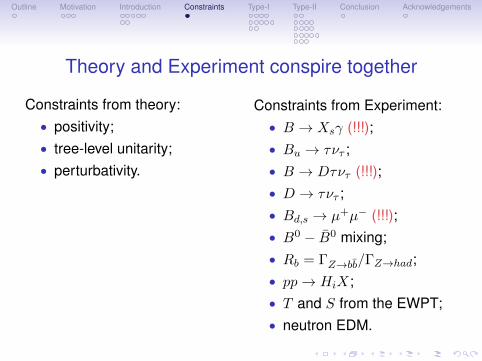
Constraints from theory:• positivity;• tree-level unitarity;• perturbativity.

Constraints from Experiment:• B → Xsγ (!!!);• Bu → τντ ;• B → Dτντ (!!!);• D → τντ ;• Bd,s → µ+µ− (!!!);• B0 − B̄0 mixing;• Rb = ΓZ→bb̄/ΓZ→had;• pp→ HiX;• T and S from the EWPT;• neutron EDM.


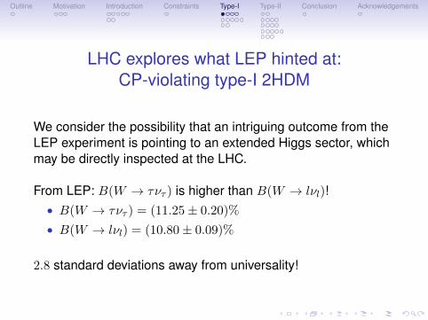
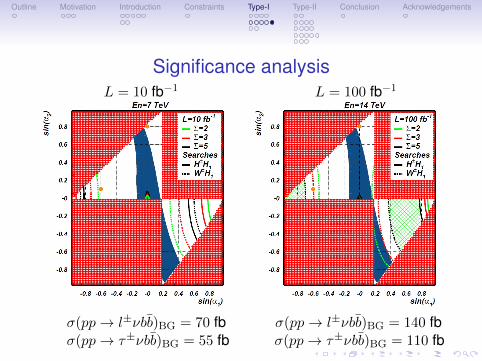
LHC explores what LEP hinted at:CP-violating type-I 2HDM

We consider the possibility that an intriguing outcome from theLEP experiment is pointing to an extended Higgs sector, whichmay be directly inspected at the LHC.

From LEP: B(W → τντ ) is higher than B(W → lνl)!• B(W → τντ ) = (11.25± 0.20)%

• B(W → lνl) = (10.80± 0.09)%

2.8 standard deviations away from universality!


The key idea

We assume that the deviation from lepton non-universality isdue to a pair-produced light Charged Higgs.

This is possible if MH± ∼MW .

The severe constraints allow only a type-I 2HDM:• all the H±ff couplings are proportional to tanβ−1;• by tuning tanβ−1 to be large, MH± can be ∼MW .

Constraints from top-associated processes are evaded as well!


A stringent assumption

If we want to explain lepton non-universality in this way, then:

• we must have a light Charged Higgs;• we must pick the Type-I 2HDM among the other typologies;• we must have a large tanβ.

This already addresses our choice of benchmark points in aspecific corner of the parameter space.

Plus, we assume that M1 = 125 GeV.


Benchmarks

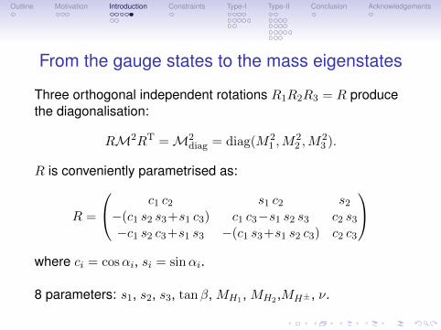
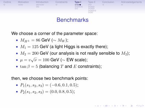
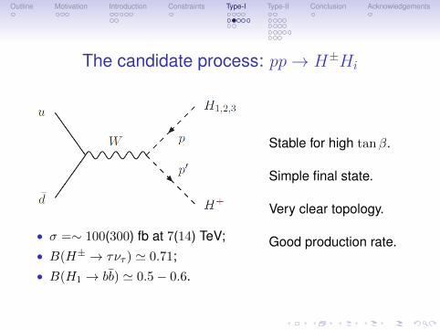
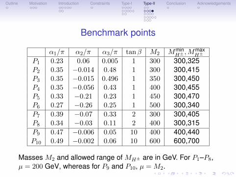
We choose a corner of the parameter space:• MH± = 86 GeV (∼MW );• M1 = 125 GeV (a light Higgs is exactly there);• M2 = 200 GeV (our analysis is not really sensible to M2);• µ = v

√ν = 100 GeV (∼ EW scale);

• tanβ = 5 (balancing T and E constraints);

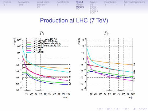
then, we choose two benchmark points:• P1(s1, s2, s3) = (−0.6, 0.1, 0.5);• P2(s1, s2, s3) = (0.0, 0.8, 0.5);


Production at LHC (7 TeV)

P1 P2


The candidate process: pp→ H±Hi

• σ =∼ 100(300) fb at 7(14) TeV;• B(H± → τντ ) ' 0.71;• B(H1 → bb̄) ' 0.5− 0.6.

Stable for high tanβ.

Simple final state.

Very clear topology.

Good production rate.


Light Higgs Branching Ratios

A closer look to γγ.Enhancement due to the Charged Higgs loop!


Selection cuts: Atlas people said. . .

pT (b), pT (τ) > 25 GeV,

|η(b)|, |η(τ)| < 2.5,

pT (ν) > 20 GeV,

|η(ν)| < 4.5,

M(b, b̄) = M1 ± 10 GeV,

100% reconstruction efficiency for τ ’s,

∼ 70% b-tagging efficiency.

And we obey. . .


Significance analysisL = 10 fb−1 L = 100 fb−1

σ(pp→ l±νbb̄)BG = 70 fb σ(pp→ l±νbb̄)BG = 140 fbσ(pp→ τ±νbb̄)BG = 55 fb σ(pp→ τ±νbb̄)BG = 110 fb


H → γγ with µ = 100 GeV

Despite an overall suppression, the γγ channel can be SM -like.


H → γγ with µ = 180 GeV

By tuning µ, γγ rate could become equal to the SM one.


Probing the charged Higgs boson at the LHC

Why CP-violating 2HDM type-II?• Strong connection with a tree-level MSSM Higgs sector;• CP-violation could be induced by loop corrections to the

Higgs potential;

It is possible that the Higgs sector lies in a lower mass rangethan the super-partners of the SM contents and can beaccessible by the LHC. In this regard, a type-II 2HDM should beexplored as an effective low-energy MSSM-like Higgs sector.

If this is true, we have a charged Higgs just around thecorner. . .


Three steps towards the Charged Higgs

The phenomenological analysis focuses on:

1. the CP-violating parameter space in the light of theoreticalarguments and experimental data (up to the newest LHCresults);

2. the profiling of the Charged Higgs in surviving portions ofthe parameter space;

3. a strategy to discover a charged Higgs associated with aW and decaying in a Wbb final state at tanβ ∼ O(1).


Allowed parameter space (1)

Red: before LHCGreen: after LHC




The surviving parameter space sits in a very small corner.

Outside a small relatively stable region, the allowed points layin a considerably fine-tuned choice of parameters.





Benchmark points

α1/π α2/π α3/π tanβ M2 MminH± ,M

maxH±

P1 0.23 0.06 0.005 1 300 300,325P2 0.35 −0.014 0.48 1 300 300,415P3 0.35 −0.015 0.496 1 350 300,450P4 0.35 −0.056 0.43 1 400 300,455P5 0.33 −0.21 0.23 1 450 300,470P6 0.27 −0.26 0.25 1 500 300,340P7 0.39 −0.07 0.33 2 300 300,405P8 0.34 −0.03 0.11 2 400 300,315P9 0.47 −0.006 0.05 10 400 400,440P10 0.49 −0.002 0.06 10 600 600,700

Masses M2 and allowed range of MH± are in GeV. For P1–P8,µ = 200 GeV, whereas for P9 and P10, µ = M2.


Charged Higgs Branching Ratios (1)


Charged Higgs Branching Ratios (2)


Charged Higgs production mechanisms (1)


Charged Higgs production mechanisms (2)


pp→ H±W∓: significance analysis

The idea is to use the light Neutral Higgs as a portal for theCharged Higgs discovery in order to avoid the enormous tt̄background.

For this we consider the final state:W∓H± →W∓W±H1 →W∓W±bb̄→ 2j + 2b+ 1`+ METproduced at 14 TeV, with a luminosity of L = 100 fb−1.

Among the possible decay patterns of the two W bosons, thesemi-leptonic one was chosen, allowing the full reconstructionof the events.


Selection cuts (1)1) Kinematics: standard detector cuts

pT` > 15 GeV, |η`| < 2.5,

pTj > 20 GeV, |ηj | < 3,

|∆Rjj | > 0.5, |∆R`j | > 0.5;

with η the pseudo-rapidity and ∆R =√

(∆η)2 + (∆φ)2.2) Light Higgs reconstruction:∣∣M(bb)− 125 GeV

∣∣ < 20 GeV ;

3) hadronic W reconstruction (Wh → jj):

|M(jj)− 80 GeV| < 20 GeV .


Selection cuts (2)

4) Top veto: if ∆R(b1,Wh) < ∆R(b2,Wh), then

M(b1jj) > 200 GeV , MT (b2`ν) > 200 GeV ,

otherwise 1↔ 2;5) same-hemisphere b quarks:

pb1|pb1 |

· pb2|pb2 |

> 0 .

After this set of cuts, the significance timidly grows (∼ 2).

It is not enough: we need a strategic cut.


Strategic cut (1)

Single cut

or

Square cut?


Strategic cut (2)

We define a single cut and a square cut:

Csqu = max(M(bbjj),MT (bb`ν)

)> Mlim

Csng = MT (bb`ν) > Mlim .

When Mlim = 600 GeV the significance reaches the best value.

Finally, if we define a further cut on the peak:

|M −MH± | < 50 GeV ,

we find that Csng is always better than Csqu.


Results: P3

√s = 14 TeV


Results: P4

√s = 14 TeV


Results: P5

√s = 14 TeV


Conclusion

We have studied the phenomenology of the Charged Higgsin two typologies of 2HDM.√

Type-I: starting from a tension between the SM and data(apparent deviation from lepton universality at LEP), wehave suggested a way to explain it (an on-shellproduced light Charged Higgs) and we have proposed amethod to test this hypothesis at the LHC.

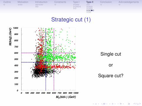
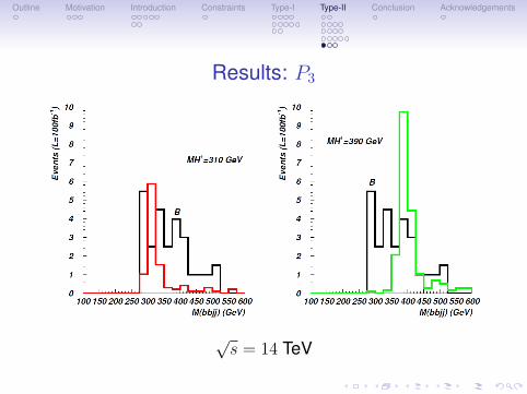
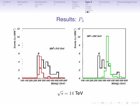
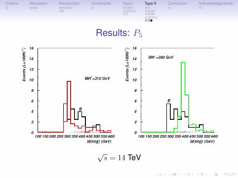
√Type-II: assuming an MSSM-like Higgs sector, we haveanalysed the surviving parameter space (in the light ofthe latest LHC data), then we have profiled the ChargedHiggs in such a scenario, finally we have proposed astrategy for discovering this particle at the LHC.


Acknowledgements

This talk is mainly based on two articles:• arXiv:1205.2692 (type-I) in collaboration with

• W. Mader,• J. Park,• D. Stöckinger,• A. Straessner;

• arXiv:1205.6569 (type-II) in collaboration with• L. Basso,• A. Lipniacka,• F. Mahmoudi,• S. Moretti,• P. Osland,• M. Purmohammadi.


Positivity

In order to have a stable potential, we impose positivity:V (Φ1,Φ2) > 0 as |Φ1|, |Φ2| → ∞.PRD 18 (1978) 2574, PLB 449 (1999) 89, PLB 471 (1999) 182

Additionally, we must insist on the hyerarchy: M2 ≤M3.In general, the minimum of the potential could be either local orglobal. However, if a local charge-conserving minimum existsthen there can be no charge-breaking minimum.PLB 603 (2004) 219, PLB 632 (2006) 684, PLB 652 (2007) 181

Nevertheless, the potential of the 2HDM can have more thanone charge-conserving minimum. We therefore check that theminimum obtained is the global one, following the approach ofRef. JHEP 1106 (2011) 003.


Tree-level unitarity

We also impose tree-level unitarity on Higgs–Higgs scattering.PLB 313 (1993) 155, PLB 490 (2000) 119,PRD 72 (2005) 115010

These conditions have a rather dramatic effect at “large” valuesof tanβ and MH± , though some tuning of µ can extend theallowed range to larger values of tanβ(PRD 84 (2011) 055028).


Perturbativity

We impose the following upper bound on all λ’s:

|λi| < 4πξ, (1)

with ξ = 0.8, meaning |λi| ≤ 10. The effect of this is to restrictlarge values of the masses, unless the soft parameter µ iscomparable to M2 and MH± .

For illustrations of how these theory constraints cut into theparameter space, see Refs. NPB 775 (2007) 45,NPCS 10 (2007) 347.


B → XsγThis FCNC inclusive decay receives contributions from thecharged Higgs boson that can be comparable to the W±

contribution. Charged Higgs state always contributes positivelyto the corresponding BR. The most up-to-date SM prediction forthis decay, at the Next-to-Next-to-Leading Order (NNLO), gives:

BR(B̄→ Xsγ)SM = (3.11± 0.22)× 10−4, (2)

while the combined experimental value from HFAG points to alarger value:

BR(B̄→ Xsγ)exp = (3.55± 0.24± 0.09)× 10−4. (3)

For type-II Yukawa interactions light charged Higgs bosons areexcluded by this observable. The actual limit is sensitive tohigher-order QCD effects and is of the order of 380 GeV, beingmore severe at low values of tanβ.


Bu → τντIn contrast to the b→ sγ transitions the process Bu → τντ canbe mediated by H± already at tree level. The 2HDMcontribution factorises in the ratio RBτν as compared to the SMvalue. The SM BR evaluates numerically to:

BR(Bu → τντ )SM = (1.01± 0.29)× 10−4. (4)

The SM prediction is compared to the current HFAG value:

BR(Bu → τντ )exp = (1.64± 0.34)× 10−4 (5)

by forming the ratio

RexpBτν ≡

BR(Bu → τντ )exp

BR(Bu → τντ )SM= 1.63± 0.54. (6)

In the framework of the 2HDM this leads to the exclusion of twosectors of the ratio tanβ/MH± .


B → DτντCompared to Bu → τντ , B → D`ν have the advantage ofdepending on |Vcb|, which is known to greater precision than|Vub|. The experimental determination remains however verycomplicated due to the presence of at least two neutrinos in thefinal state. The ratio

ξD`ντ =BR(B → Dτντ )

BR(B → Deνe), (7)

allows one to reduce the theoretical uncertainties. The SMprediction is:

ξSMD`ν = (29.7± 3)× 10−2, (8)

and the most recent experimental result by the BaBarcollaboration is:

ξexpD`ν = (41.6± 11.7± 5.2)× 10−2. (9)

This is complementary to Bu → τντ .


Ds → τντ

Constraints on a light charged Higgs can be obtained,competitive with those obtained from Bu → τντ . The mainuncertainty here is due to the decay constant fDs . The SMprediction for this decay is:

BR(Ds → τντ )SM = (5.11± 0.13)× 10−2, (10)

using fDs = 248± 2.5 MeV, and the current world average ofthe experimental measurements gives:

BR(Ds → τντ )exp = (5.38± 0.32)× 10−2. (11)


Bd,s → µ+µ−

These decays are helicity suppressed in the SM and canreceive sizeable enhancement or depletion fromHiggs-mediated contributions. At large tanβ, thenon-observation of these decay modes imposes a lower boundon the charged Higgs boson mass. The most stringent limits fortheir BRs were reported by the LHCb collaboration:

BR(Bs → µ+µ−) < 4.5× 10−9, (12)BR(Bd → µ+µ−) < 1.0× 10−9, (13)

at 95% C.L., while the SM prediction is:

BR(Bs → µ+µ−) = (3.53± 0.38)× 10−9, (14)BR(Bd → µ+µ−) = (0.11± 0.01)× 10−9, (15)

with Bs being the more constraining. In the type-II 2HDM, theexperimental limits can be reached for large values of theYukawa couplings and small charged Higgs boson masses.


B0 − B̄0 mixing

Due to the possibility of H± exchange, in addition to Wexchange, the B0 − B̄0 mixing constraint, which is sensitive tothe term mt cotβ in the Yukawa couplings, excludes low valuesof tanβ and low values of MH± .

The non-perturbative decay constant fBd and the bagparameter B̂d which are evaluated simultaneously from latticeQCD constitute the largest theoretical uncertainty.


Rb = ΓZ→bb̄/ΓZ→had

The branching ratio Rb ≡ ΓZ→bb̄/ΓZ→had would also be affectedby Higgs boson exchange.

The contributions from neutral Higgs bosons to Rb arenegligible, however, charged Higgs boson contributions, via theH±bt Yukawa coupling, exclude low values of tanβ and lowMH± .


T and S from the EWPT

For the electroweak “precision observables” T and S, weimpose the bounds |∆T | < 0.10, |∆S| < 0.10, at the 1-σ level,within the framework of Refs. JPG 35 (2008) 075001,NPB 801 (2008) 81.

While S is not very restrictive, T gets a positive contributionfrom a splitting between the masses of charged and neutralHiggs bosons, whereas a pair of neutral ones give a negativecontribution.


EDM of the Neutron

The bound on the electron EDM constrains the allowed amountof CP violation of the model. We adopt the bound:

|de| ≤ 1× 10−27[e cm], (16)

at the 1-σ level. The contribution due to neutral Higgsexchange, via the two-loop Barr–Zee effect, is given byEq. (3.2) of NPB 644 (2002) 263.

Date post:	03-Apr-2018
Category:	Documents
Upload:	truongxuyen
View:	223 times
Download:	2 times

CP-violating two-Higgs-doublet Model and charged … · CP-violating two-Higgs-doublet Model and...

Documents