1 CPC: Complementary Progress Constraints for Time-Optimal Quadrotor Trajectories Philipp Foehn, Davide Scaramuzza Abstract—In many mobile robotics scenarios, such as drone racing, the goal is to generate a trajectory that passes through multiple waypoints in minimal time. This problem is referred to as time-optimal planning. State-of-the-art approaches either use polynomial trajectory formulations, which are suboptimal due to their smoothness, or numerical optimization, which requires way- points to be allocated as costs or constraints to specific discrete- time nodes. For time-optimal planning, this time-allocation is a priori unknown and renders traditional approaches incapable of producing truly time-optimal trajectories. We introduce a novel formulation of progress bound to waypoints by a com- plementarity constraint. While the progress variables indicate the completion of a waypoint, change of this progress is only allowed in local proximity to the waypoint via complementarity constraints. This enables the simultaneous optimization of the trajectory and the time-allocation of the waypoints. To the best of our knowledge, this is the first approach allowing for truly time- optimal trajectory planning for quadrotors and other systems. We perform and discuss evaluations on optimality and convexity, compare to other related approaches, and qualitatively to an expert-human baseline. I. I NTRODUCTION Autonomous aerial vehicles are nowadays being used for inspection, delivery, cinematography, search-and-rescue, and recently even drone racing. The most prominent aerial system is the quadrotor, thanks to its vertical take-off and hover capabilities, its simplicity, and its versatility ranging from smooth maneuvers to extremely aggressive trajectories. How- ever, quadrotors have limited range dictated by their battery capacity, which in turn limits how much time can be spent on a specific task. If the tasks consists of visiting multiple waypoints (delivery, inspection, drone racing [1, 2]), doing so in minimal time is often viable, and in the context of search and rescue or drone racing even the ultimate goal. Truly time-optimal quadrotor trajectories exploit the full actuator potential at every point in time, which excludes using continuous polynomial formulations due to their inherent smoothness. This leaves planning time-discretized trajectories as the only option, which is typically solved using numerical optimization. Unfortunately, such formulations require the al- location of waypoints as costs or constraints to specific discrete time nodes, which is a priori unknown. We investigate this problem and provide a solution that allows to simultaneously optimize the trajectory and waypoint allocation. Our approach formulates a progress measure for each waypoint along the trajectory, indicating completion of a waypoint (see Fig. 1). We then introduce a complementary progress constraint, that allows completion only in proximity to a waypoint. For simple point-mass systems, time-optimal trajectories can be computed in closed-form resulting in bang-bang accel- State-of-the-Art: Waypoint Allocation using Constraints Our Method: Waypoint Progress Variables λ and their Completion (Arrows) Fig. 1: Top: state-of-the-art fixed allocation of waypoints to specific nodes. Bottom: our method of defining one progress variable per waypoint. The progress variable can switch from 1 (incomplete) to 0 (completed) only when in proximity of the relevant waypoint, implemented as a complementary constraint (details in Fig. 3). eration trajectories, which can easily be sampled over multiple waypoints. However, quadrotors are underactuated systems that need to rotate to adjust their acceleration direction, which always lies in the body z-axis. Both the linear and rotational acceleration are controlled through the rotor thrusts, which are physically limited by the actuators. This introduces a coupling in the achievable linear and rotational accelerations. Therefore, time-optimal planning becomes the search for the optimal tradeoff between maximizing these accelerations. There exist two approaches in formulating the underlying state space for trajectory planning: (i) polynomial representa- tions and (ii) discretized state space formulations. The first approach exploits the quadrotor’s differentially-flat output states represented by smooth polynomials. Their com- putation is extremely efficient and trajectories through multiple waypoints can be represented by concatenating polynomial segments, where sampling over segment times and boundary conditions provides minimal-time solutions. However, these polynomial, minimal-time solutions are still suboptimal for quadrotors, since they (i) are smooth and cannot represent rapidly-changing states, such as bang-bang trajectories, and (ii) can only touch the constant boundaries in infinitesimal points, but never stay at the limit for durations different than the total segment time. Both problems are visualized in Fig. 2 and further explained in Sec. II. The second approach uses non-linear optimization to plan trajectories described by a time-discretized state space, where the system dynamics and input boundaries are enforced as constraints. In contrast to the polynomial formulation, this allows the optimization to pick any input within bounds for each discrete time step. For a time-optimal solution, the tra- jectory time t N is part of the optimization variables and is the
Abstract—In many mobile robotics scenarios, such as droneracing, the goal is to generate a trajectory that passes throughmultiple waypoints in minimal time. This problem is referred toas time-optimal planning. State-of-the-art approaches either usepolynomial trajectory formulations, which are suboptimal due totheir smoothness, or numerical optimization, which requires way-points to be allocated as costs or constraints to specific discrete-time nodes. For time-optimal planning, this time-allocation is apriori unknown and renders traditional approaches incapableof producing truly time-optimal trajectories. We introduce anovel formulation of progress bound to waypoints by a com-plementarity constraint. While the progress variables indicatethe completion of a waypoint, change of this progress is onlyallowed in local proximity to the waypoint via complementarityconstraints. This enables the simultaneous optimization of thetrajectory and the time-allocation of the waypoints. To the best ofour knowledge, this is the first approach allowing for truly time-optimal trajectory planning for quadrotors and other systems.We perform and discuss evaluations on optimality and convexity,compare to other related approaches, and qualitatively to anexpert-human baseline.
I. INTRODUCTION
Autonomous aerial vehicles are nowadays being used forinspection, delivery, cinematography, search-and-rescue, andrecently even drone racing. The most prominent aerial systemis the quadrotor, thanks to its vertical take-off and hovercapabilities, its simplicity, and its versatility ranging fromsmooth maneuvers to extremely aggressive trajectories. How-ever, quadrotors have limited range dictated by their batterycapacity, which in turn limits how much time can be spenton a specific task. If the tasks consists of visiting multiplewaypoints (delivery, inspection, drone racing [1, 2]), doing soin minimal time is often viable, and in the context of searchand rescue or drone racing even the ultimate goal.
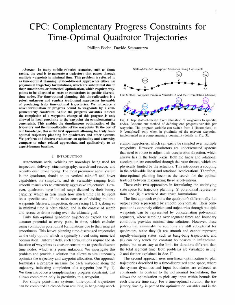
Truly time-optimal quadrotor trajectories exploit the fullactuator potential at every point in time, which excludesusing continuous polynomial formulations due to their inherentsmoothness. This leaves planning time-discretized trajectoriesas the only option, which is typically solved using numericaloptimization. Unfortunately, such formulations require the al-location of waypoints as costs or constraints to specific discretetime nodes, which is a priori unknown. We investigate thisproblem and provide a solution that allows to simultaneouslyoptimize the trajectory and waypoint allocation. Our approachformulates a progress measure for each waypoint along thetrajectory, indicating completion of a waypoint (see Fig. 1).We then introduce a complementary progress constraint, thatallows completion only in proximity to a waypoint.
For simple point-mass systems, time-optimal trajectoriescan be computed in closed-form resulting in bang-bang accel-
State-of-the-Art: Waypoint Allocation using Constraints
Our Method: Waypoint Progress Variables λ and their Completion (Arrows)
Fig. 1: Top: state-of-the-art fixed allocation of waypoints to specificnodes. Bottom: our method of defining one progress variable perwaypoint. The progress variable can switch from 1 (incomplete) to0 (completed) only when in proximity of the relevant waypoint,implemented as a complementary constraint (details in Fig. 3).
eration trajectories, which can easily be sampled over multiplewaypoints. However, quadrotors are underactuated systemsthat need to rotate to adjust their acceleration direction, whichalways lies in the body z-axis. Both the linear and rotationalacceleration are controlled through the rotor thrusts, which arephysically limited by the actuators. This introduces a couplingin the achievable linear and rotational accelerations. Therefore,time-optimal planning becomes the search for the optimaltradeoff between maximizing these accelerations.
There exist two approaches in formulating the underlyingstate space for trajectory planning: (i) polynomial representa-tions and (ii) discretized state space formulations.
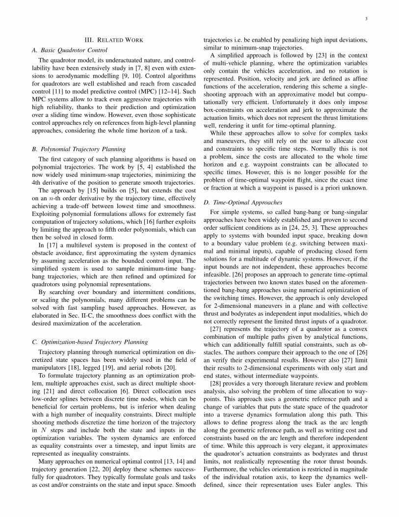
The first approach exploits the quadrotor’s differentially-flatoutput states represented by smooth polynomials. Their com-putation is extremely efficient and trajectories through multiplewaypoints can be represented by concatenating polynomialsegments, where sampling over segment times and boundaryconditions provides minimal-time solutions. However, thesepolynomial, minimal-time solutions are still suboptimal forquadrotors, since they (i) are smooth and cannot representrapidly-changing states, such as bang-bang trajectories, and(ii) can only touch the constant boundaries in infinitesimalpoints, but never stay at the limit for durations different thanthe total segment time. Both problems are visualized in Fig.2 and further explained in Sec. II.
The second approach uses non-linear optimization to plantrajectories described by a time-discretized state space, wherethe system dynamics and input boundaries are enforced asconstraints. In contrast to the polynomial formulation, thisallows the optimization to pick any input within bounds foreach discrete time step. For a time-optimal solution, the tra-jectory time tN is part of the optimization variables and is the
2
sole term in the cost function. However, if multiple waypointsmust be passed, these must be allocated as constraints tospecific nodes on the trajectory. Since the fraction of overalltime spent between any two waypoints is unknown, it isa priori undefined to which nodes on the trajectory suchwaypoint constraints should be allocated. This problem renderstraditional discretized state space formulations ineffective fortime-optimal trajectory generation through multiple waypoints.
In this work, we answer the following research questions:1) How can we revise the waypoint constraints to optimize
simultaneously time-allocation, while exploiting the sys-tem dynamics and actuation limits?
2) What are the resulting properties regarding initializationand convergence due to (non-) convex constraints?
3) What are the characteristics of time-optimal trajectories?
Contribution
Our approach optimizes a time-discretized state and inputspace for minimum execution time, with the quadrotor dynam-ics and input bounds implemented as equality and inequalityconstraints, respectively. Our contribution is a formulationof progress over the trajectory, where the completion of awaypoint is represented as a progress variable (see Fig. 1).We introduce a complementarity constraint, which allows theprogress variable of a waypoint to switch from incomplete tocomplete only at the time nodes where the vehicle is withintolerance of the waypoint. This allows us to encapsulate thetask of reaching multiple waypoints without specifying atwhich time a waypoint is reached, solving the time-allocationproblem. We evaluate our approach experimentally in a multi-tude of scenarios, covering basic optimality and convergencetests, verifying time alignment of waypoints, many-waypointscenarios, and finally comparing against human performance.
II. PREFACE: TIME-OPTIMAL QUADROTOR TRAJECTORY
A. Point-Mass Bang-Bang
Time-optimal trajectories encapsulate the best possible ac-tion to reach one or multiple targets in the lowest possible time.We first investigate a point mass in R3 controlled by boundedacceleration a ∈ R3 | ‖a‖ ≤ amax, starting at rest position p0and translating to rest position p1. The time-optimal solutiontakes the form of a bang-bang trajectory over the time topt,accelerating with amax for topt/2, followed by deceleratingwith amax for topt/2. A trajectory through multiple waypointscan be generated similarly by optimizing over the switchingtimes and intermittent waypoint velocities. For the generalsolution and applications we refer to [3].
B. Bang-Bang Relation for Quadrotors
A quadrotor would exploit the same maximal accelerationby generating the maximal possible thrust with its rotors.However, due to the quadrotor’s underactuation, it can notinstantaneously change the acceleration direction, but needs torotate by applying differential thrust over its rotors. The linearand rotational acceleration are both controlled through therotor thrusts, which in turn are limited, introducing a coupling
0.0 0.5 1.0 1.5 2.0
0
2
4
6
p[m
]
9th ordert = 2.165s
7th ordert = 1.938s
5th ordert = 1.699s
bang-bangt = 1.614s
0.0 0.5 1.0 1.5 2.0 t [s]−10
−5
0
5
10
a[m/s
2 ]
amax
−amax
Fig. 2: Multiple orders of polynomial trajectories and one bang-bangtrajectory with limited slope. The polynomial trajectories only touchthe input extrema in two points, while the bang-bang spends moretime at the limit and achieves a lower overall time.
of the achievable linear and rotational acceleration (visualizedlater in Fig. 4). Therefore, a time-optimal trajectory is theoptimal tradeoff between rotational and linear acceleration,where the rotor thrusts only deviate from the maximum toadjust the rotational rates. Indeed, our experiments confirmexactly this behavior (see e.g. Fig, 5), as in Sec. VIII.
C. Sub-Optimality of Polynomial Trajectories
The quadrotor is a differentially flat system [4] that can bedescribed based on its four flat output states, position and yaw.This allows to represent the evolution of the flat output statesas smooth differentiable polynomials of the time t. To generatesuch polynomials, one typically defines its boundary condi-tions at start and end time, and solves for a smooth polynomial,optionally minimizing one of the derivatives, commonly thesnap (4th derivative of position, as in [5]). The intentionbehind such minimum-snap trajectories is to minimize andsmooth the needed body torques and, therefore, single motorthrust differences, which are dependent on the snap. Since thepolynomials are extremely efficient to compute, trajectoriesthrough many waypoints can be generated by concatenatingsegments of polynomials, and minimal-time solutions can befound by optimizing or sampling over the segment times andboundary conditions. However, these polynomials are smoothby definition, which stands in direct conflict with maximizingthe acceleration at all times while simultaneously adapting therotational rate, as explained in the previous Sec. II-B. In fact,due to the polynomial nature of the trajectories, the boundariesof the reachable input spaces can only be touched at one ormultiple points, or constantly, but not at subsegments of thetrajectory. This problem is visualized in Fig. 2, and not onlyapplies to polynomial trajectories, but partially also to directcollocation methods for optimization [6].
D. Real-World Deployment
Note that the time optimal solutions cannot be tracked on areal system, because disturbances could not be corrected, sincethe system is at the boundary of the reachable input space [3].
3
III. RELATED WORK
A. Basic Quadrotor Control
The quadrotor model, its underactuated nature, and control-lability have been extensively study in [7, 8] even with exten-sions to aerodynamic modelling [9, 10]. Control algorithmsfor quadrotors are well established and reach from cascadedcontrol [11] to model predictive control (MPC) [12–14]. SuchMPC systems allow to track even aggressive trajectories withhigh reliability, thanks to their prediction and optimizationover a sliding time window. However, even those sophisticatecontrol approaches rely on references from high-level planningapproaches, considering the whole time horizon of a task.
B. Polynomial Trajectory Planning
The first category of such planning algorithms is based onpolynomial trajectories. The work by [5, 4] established thenow widely used minimum-snap trajectories, minimizing the4th derivative of the position to generate smooth trajectories.
The approach by [15] builds on [5], but extends the coston an n-th order derivative by the trajectory time, effectivelyachieving a trade-off between lowest time and smoothness.Exploiting polynomial formulations allows for extremely fastcomputation of trajectory solutions, which [16] further exploitsby limiting the approach to fifth order polynomials, which canthen be solved in closed form.
In [17] a multilevel system is proposed in the context ofobstacle avoidance, first approximating the system dynamicsby assuming acceleration as the bounded control input. Thesimplified system is used to sample minimum-time bang-bang trajectories, which are then refined and optimized forquadrotors using polynomial representations.
By searching over boundary and intermittent conditions,or scaling the polynomials, many different problems can besolved with fast sampling based approaches. However, aselaborated in Sec. II-C, the smoothness does conflict with thedesired maximization of the acceleration.
C. Optimization-based Trajectory Planning
Trajectory planning through numerical optimization on dis-cretized state spaces has been widely used in the field ofmanipulators [18], legged [19], and aerial robots [20].
To formulate trajectory planning as an optimization prob-lem, multiple approaches exist, such as direct multiple shoot-ing [21] and direct collocation [6]. Direct collocation useslow-order splines between discrete time nodes, which can bebeneficial for certain problems, but is inferior when dealingwith a high number of inequality constraints. Direct multipleshooting methods discretize the time horizon of the trajectoryin N steps and include both the state and inputs in theoptimization variables. The system dynamics are enforcedas equality constraints over a timestep, and input limits arerepresented as inequality constraints.
Many approaches on numerical optimal control [13, 14] andtrajectory generation [22, 20] deploy these schemes success-fully for quadrotors. They typically formulate goals and tasksas cost and/or constraints on the state and input space. Smooth
trajectories i.e. be enabled by penalizing high input deviations,similar to minimum-snap trajectories.
A simplified approach is followed by [23] in the contextof multi-vehicle planning, where the optimization variablesonly contain the vehicles acceleration, and no rotation isrepresented. Position, velocity and jerk are defined as affinefunctions of the acceleration, rendering this scheme a single-shooting approach with an approximative model but compu-tationally very efficient. Unfortunately it does only imposebox-constraints on acceleration and jerk to approximate theactuation limits, which does not represent the thrust limitationswell, rendering it unfit for time-optimal planning.
While these approaches allow to solve for complex tasksand maneuvers, they still rely on the user to allocate costand constraints to specific time steps. Normally this is nota problem, since the costs are allocated to the whole timehorizon and e.g. waypoint constraints can be allocated tospecific times. However, this is no longer possible for theproblem of time-optimal waypoint flight, since the exact timeor fraction at which a waypoint is passed is a priori unknown.
D. Time-Optimal ApproachesFor simple systems, so called bang-bang or bang-singular
approaches have been widely established and proven to secondorder sufficient conditions as in [24, 25, 3]. These approachesapply to systems with bounded input space, breaking downto a boundary value problem (e.g. switching between maxi-mal and minimal inputs), capable of producing closed formsolutions for a multitude of dynamic systems. However, if theinput bounds are not independent, these approaches becomeinfeasible. [26] proposes an approach to generate time-optimaltrajectories between two known states based on the aforemen-tioned bang-bang approaches using numerical optimization ofthe switching times. However, the approach is only developedfor 2-dimensional maneuvers in a plane and with collectivethrust and bodyrates as independent input modalities, which donot correctly represent the limited thrust inputs of a quadrotor.
[27] represents the trajectory of a quadrotor as a convexcombination of multiple paths given by analytical functions,which can additionally fulfill spatial constraints, such as ob-stacles. The authors compare their approach to the one of [26]an verify their experimental results. However also [27] limittheir results to 2-dimensional experiments with only start andend states, without intermediate waypoints.
[28] provides a very thorough literature review and problemanalysis, also solving the problem of time allocation to way-points. This approach uses a geometric reference path and achange of variables that puts the state space of the quadrotorinto a traverse dynamics formulation along this path. Thisallows to define progress along the track as the arc lengthalong the geometric reference path, as well as writing cost andconstraints based on the arc length and therefore independentof time. While this approach is very elegant, it approximatesthe quadrotor’s actuation constraints as bodyrates and thrustlimits, not realistically representing the rotor thrust bounds.Furthermore, the vehicles orientation is restricted in magnitudeof the individual rotation axis, to keep the dynamics well-defined, since their representation uses Euler angles. This
4
limits the space of solutions and therefore the optimality ofthe resulting trajectory.
Finally, [29] provides a method to generate close totime-optimal segment times for polynomial trajectories usingBayesian Optimization. The approach is based on learningGaussian Classification models predicting feasibility of atrajectory based on multi-fidelity data from analytic models,simulation and real-world data. While this approach puts highemphasis on real-world applicability and can even account foraerodynamic effects, it is still constrained to polynomials andrequires real-world data specifically collected for the givenvehicle. Furthermore, it is an approximative method rather thanthe true time-optimal solution.
IV. PROBLEM FORMULATION
A. General Trajectory OptimizationThe general optimization problem of finding the minimizer
x∗ for cost J(x) in the state space x ∈ Xn can be stated as
x∗ = minxL(x) (1)
subject to g(x) = 0 and h(x) ≤ 0
where g(x) and h(x) contain all equality and inequality con-straints respectively. The full state space x is used equivalentto the term optimization variables. The cost L(x) typicallycontains one or multiple quadratic costs on the deviation froma reference, costs on the systems actuation inputs, or othercosts describing any desired behaviors.
1) Multiple Shooting Method: To represent a dynamicsystem in the state space, the system state xk is describedat discrete times tk = dt ∗ k at k ∈ (0, N), also called nodes,where its actuation inputs between two nodes are uk at tk withk ∈ (0, N ]. The systems evolution is defined by the dynamicsfdyn(x,u) = x, anchored at x0 = xinit, and implementedas an equality constraint of the first order forward integration:
xk+1 − xk − dt · fdyn(xk,uk) = 0 (2)
which is part of g(x) = 0 in the general formulation. Bothxk, uk are part of the state space and can be summarized asthe vehicles dynamic states xdyn,k at node k.
2) Integration Scheme: Additionally we can change the for-mulation to use a higher order integration scheme to suppresslinearization errors for highly non-linear systems. In this work,we deploy a 4th order Runge-Kutta scheme:
B. Time-Optimal Trajectory OptimizationOptimizing for a time-optimal trajectory means that the only
cost term is the overall trajectory time L(x) = tN . Therefore,tN needs to be in the optimization variables x = [tN , . . . ]
ᵀ,and must be positive tN > 0. The integration scheme can thenbe adapted to use dt = tN/N .
C. Passing Waypoints through Optimization
To generate trajectories passing through a sequence ofwaypoints pwj with j ∈ [0, . . . ,M ] called track, one wouldtypically define a distance cost or constraint and allocate it toa specific state xdyn,k at node k with time tk. For cost-basedformulations, quadratic distance costs are robust in terms ofconvergence and implemented as
Ldist,j = (pk − pwj)ᵀ(pk − pwj) (5)
where pk, part of x, is the position state at a user definedtime tk. However, such a cost-based formulation is only a softrequirement and if summed with other cost terms does notimply that the waypoint is actually passed within a certaintolerance. To guarantee passing within a tolerance, constraint-based formulations can be used, such as
(pk − pwj)ᵀ(pk − pwj) <= τ2j (6)
which in the general problem is part of h(x) ≤ 0, and requiresthe trajectory to pass by waypoint j at position pwj withintolerance τj at time tk.
D. The Problem of Time Allocation and Optimization
Adding waypoints to a trajectory means that their costs orconstraints need to be allocated to specific nodes (at times tk)on the trajectory. This fixes the time at which a waypoint ispassed, or even if we optimize over the total time tN , it stillfixes the fractional time tk = tN/N · k. However, it is notalways possible to know a priori how much time or whatfraction of the total time is spent between two waypoints.Therefore, it is not possible to allocate waypoint costs orconstraints to nodes at specific times.
One approach is to spread the cost of reaching the waypointover multiple nodes, which is done in [13] with an exponentialweight spread. Even though this allows to shift the time ofpassing a waypoint, the width and mean of the weight spreadare still user-defined, suboptimal in most scenarios, and doesnot allow to freely shift the time at which a waypoint is passed.
There are two possible ways to solve this: (i) changethe time between fixed nodes, which implies changing dtfor each timestep by adding all dtk to the optimizationvariables; or (ii) change the node k to which a waypointis allocated. The first option is to allow varying timetepsdtk. This however negatively impacts the linearization qualityand makes it inconsistent over the trajectory, allows trivial orsuboptimal solutions, or even leads the optimization to exploitlinearization errors. The second option requires a formulationthat allows the optimization to change the node k to whicha waypoint is allocated. Since this tackles the fundamentalunderlying allocation problem, we base our approach on thissecond option.
E. Problem Formulation Summary
In conclusion, the goal of this work is to find an opti-mization problem formulation which (i) satisfies the systemdynamics and input limitations, (ii) minimizes total trajectorytime, (iii) passes by multiple waypoints in sequence, and (iv)finds the optimal time at which to pass each waypoint.
5
V. APPROACH:COMPLEMENTARY PROGRESS CONSTRAINTS
Our approach consists of two main steps: (i) adding ameasure of progress throughout the track, and (ii) addinga measure of how this progress changes. In the followingsections we explain how these two steps can be formulatedand added to an numerical optimization problem.
A. Progress Measure Variables
To describe the progress throughout a track we want ameasure that fulfills the following requirements: (i) it starts ata defined value, (ii) it must reach a different value by the endof the trajectory, and (iii) it can only change when a waypointis passed within a certain tolerance. To achieve this, let thevector λk ∈ RM define the progress variables λjk at timesteptk for all M waypoints indexed by j. All progress variablesstart at 1 as in λ0 = 1 and must reach 0 at the end of thetrajectory as in λN = 0. The progress variables λ are chainedtogether and their evolution is defined by
λk+1 = λk − µk (7)
where the vector µk ∈ RM indicates the progress step atevery timestep. Note that the progress can only be positive,therefore µjk ≤ 0. Both λk and µk for every timestep are partof the optimization variables x, which replicates the multipleshooting scheme for the progress variables.
To define when and how the progress variables can change,we now imply constraints on µk, in it’s general form as
ε−k ≤ fprog(xk,µk) ≤ ε+k (8)
where ε−, ε+ can form equality or inequality constraints.Finally, to ensure that the waypoints are passed in the
given sequence, we enforce subsequent progress variables tobe bigger than their prequel at each timestep by
µjk ≤ µj+1k ∀k ∈ [0, N ], j ∈ [0,M). (9)
B. Complementary Progress Constraints
In the context of waypoint following, the goal is to allowµk to only be non-zero at the time of passing a waypoint.Therefore, fprog and ε− = ε+ = 0 are chosen to represent acomplementarity constraint, as
fprog(xk,µk) =[µjk · ‖pk − pwj‖22
]j∈[0,M)
!= 0 (10)
which can be interpreted as a mathematical ”or” function,since either µjk or ‖pk − pwj‖ must be 0. Intuitively, the twoelements complement each other.
C. Tolerance Relaxation
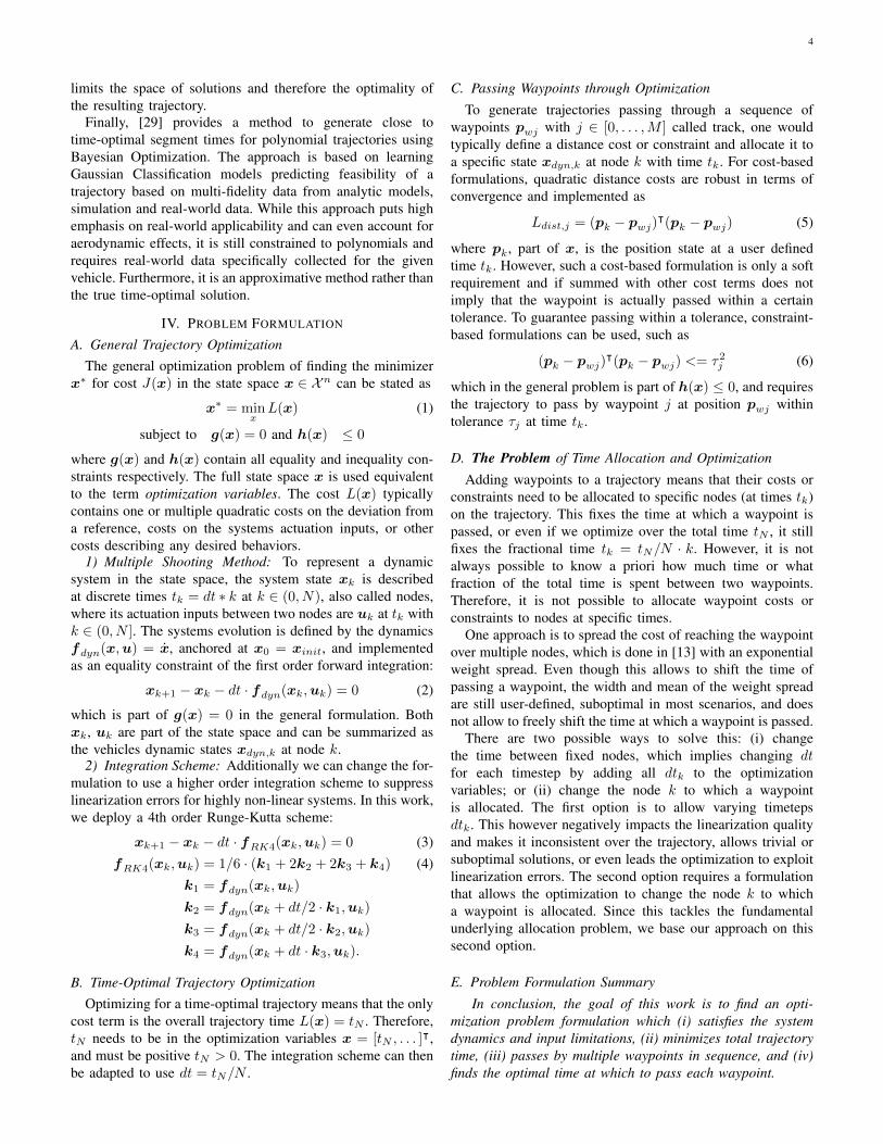
With Eqn. 10 the trajectory is forced to pass exactly througha waypoint. Not only is this impractical, since often a certaintolerance is admitted or even wanted, but it also negativelyimpacts the convergence behavior and time-optimality, sincethe system dynamics are discretized and one of the discretetimesteps must coincide with the waypoint. Therefore, it is
Fig. 3: Illustration of the Complementary Progress Constraint. µ canonly be non-zero if the distance to the waypoint pw is less than thetolerance dtol. This is not the case for x0, but for x1, and allowingthe progress variable to switch to 0 (complete).
desirable to relax a waypoint constraint by a certain tolerancewhich is achieved by extending Eqn. 10 to
fprog(xk,µk) =[µjk ·
(‖pk − pwj‖22 − νjk
)]j∈[0,M)
(11)
subject to 0 ≤ νjk ≤ d2tolwhere νjk is a slack variable to allow the distance to thewaypoint to be relaxed to zero when it is smaller than dtol,the maximal distance tolerance. This now enforces that theprogress variables can not change, except for the timesteps atwhich the system is within tolerance to the waypoint.
VI. FULL PROBLEM FORMULATION
The full space of optimization variables x consists of theoverall time and all variables assigned to nodes k as xk. Allnodes k include the robots dynamic state xdyn,k, its inputsuk, and all progress variable, therefore:
x = [tN ,x0, . . . ,xN ] (12)where
xk =
{[xdyn,k,uk,λk,µk,νk] for k ∈ [0, N)
[xdyn,N ,λN ] for k = N.(13)
Based on this representation, we write the full problem as
x∗ = minxtN (14)
subject to the system dynamics and initial constraint
the progress evolution, boundary, and sequence constraints
λk+1 − λk + µk = 0 (18)λ0 = 0 λN − 1 = 0 (19)
λjk − λj+1k ≤ 0 ∀j ∈ [0,m), (20)
and the complementarity constraint with tolerance
µjk ·(‖pk − pwj‖22 − νjk
)= 0 (21)
−νjk ≤ 0 νjk − d2tol ≤ 0. (22)
6
(a) Acceleration Space
20 10 0 10 20ax [m/s2]
30
20
10
0
10
20
a y [m
/s2 ]
g
amaxamin
a a + g
(b) Thrust and Torque Space
1.0 0.5 0.0 0.5 1.0 [Nm]
0
4
8
12
16
20
T [N
]
Tmax
Tmean
Tmin
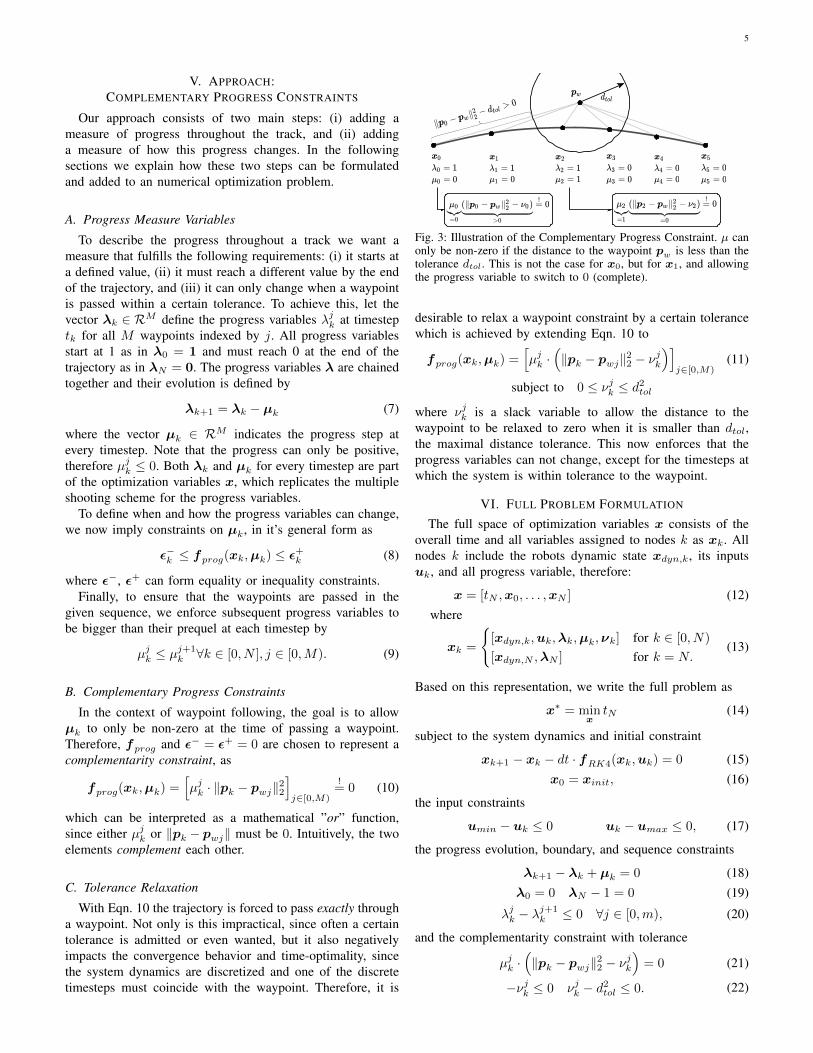
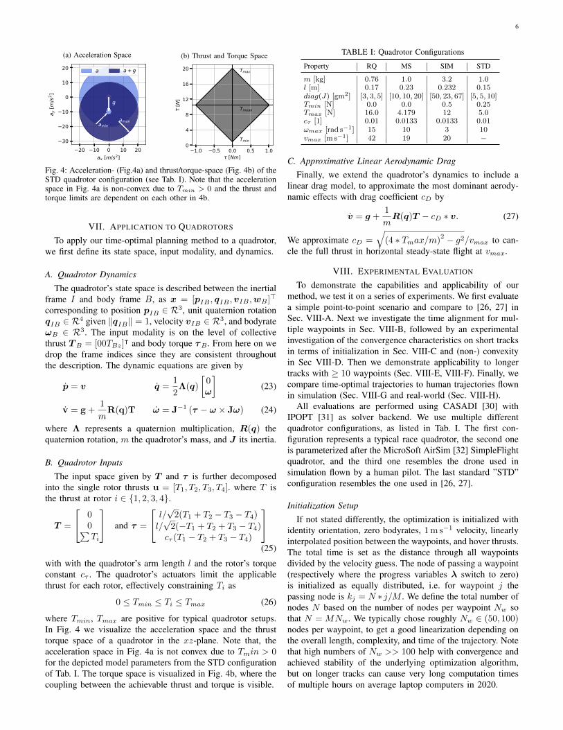
Fig. 4: Acceleration- (Fig.4a) and thrust/torque-space (Fig. 4b) of theSTD quadrotor configuration (see Tab. I). Note that the accelerationspace in Fig. 4a is non-convex due to Tmin > 0 and the thrust andtorque limits are dependent on each other in 4b.
VII. APPLICATION TO QUADROTORS
To apply our time-optimal planning method to a quadrotor,we first define its state space, input modality, and dynamics.
A. Quadrotor Dynamics
The quadrotor’s state space is described between the inertialframe I and body frame B, as x = [pIB , qIB ,vIB ,wB ]
>
corresponding to position pIB ∈ R3, unit quaternion rotationqIB ∈ R4 given ‖qIB‖ = 1, velocity vIB ∈ R3, and bodyrateωB ∈ R3. The input modality is on the level of collectivethrust TB = [00TBz]
ᵀ and body torque τB . From here on wedrop the frame indices since they are consistent throughoutthe description. The dynamic equations are given by
p = v q =1
2Λ(q)
[0ω
](23)
v = g +1
mR(q)T ω = J−1 (τ − ω × Jω) (24)
where Λ represents a quaternion multiplication, R(q) thequaternion rotation, m the quadrotor’s mass, and J its inertia.
B. Quadrotor Inputs
The input space given by T and τ is further decomposedinto the single rotor thrusts u = [T1, T2, T3, T4]. where T isthe thrust at rotor i ∈ {1, 2, 3, 4}.
T =
00∑Ti
and τ =
l/√2(T1 + T2 − T3 − T4)
l/√2(−T1 + T2 + T3 − T4)
cτ (T1 − T2 + T3 − T4)
(25)
with with the quadrotor’s arm length l and the rotor’s torqueconstant cτ . The quadrotor’s actuators limit the applicablethrust for each rotor, effectively constraining Ti as
0 ≤ Tmin ≤ Ti ≤ Tmax (26)
where Tmin, Tmax are positive for typical quadrotor setups.In Fig. 4 we visualize the acceleration space and the thrusttorque space of a quadrotor in the xz-plane. Note that, theacceleration space in Fig. 4a is not convex due to Tmin > 0for the depicted model parameters from the STD configurationof Tab. I. The torque space is visualized in Fig. 4b, where thecoupling between the achievable thrust and torque is visible.
Finally, we extend the quadrotor’s dynamics to include alinear drag model, to approximate the most dominant aerody-namic effects with drag coefficient cD by
v = g +1
mR(q)T − cD ∗ v. (27)
We approximate cD =
√(4 ∗ Tmax/m)
2 − g2/vmax to can-cle the full thrust in horizontal steady-state flight at vmax.
VIII. EXPERIMENTAL EVALUATION
To demonstrate the capabilities and applicability of ourmethod, we test it on a series of experiments. We first evaluatea simple point-to-point scenario and compare to [26, 27] inSec. VIII-A. Next we investigate the time alignment for mul-tiple waypoints in Sec. VIII-B, followed by an experimentalinvestigation of the convergence characteristics on short tracksin terms of initialization in Sec. VIII-C and (non-) convexityin Sec VIII-D. Then we demonstrate applicability to longertracks with ≥ 10 waypoints (Sec. VIII-E, VIII-F). Finally, wecompare time-optimal trajectories to human trajectories flownin simulation (Sec. VIII-G and real-world (Sec. VIII-H).
All evaluations are performed using CASADI [30] withIPOPT [31] as solver backend. We use multiple differentquadrotor configurations, as listed in Tab. I. The first con-figuration represents a typical race quadrotor, the second oneis parameterized after the MicroSoft AirSim [32] SimpleFlightquadrotor, and the third one resembles the drone used insimulation flown by a human pilot. The last standard ”STD”configuration resembles the one used in [26, 27].
Initialization Setup
If not stated differently, the optimization is initialized withidentity orientation, zero bodyrates, 1m s−1 velocity, linearlyinterpolated position between the waypoints, and hover thrusts.The total time is set as the distance through all waypointsdivided by the velocity guess. The node of passing a waypoint(respectively where the progress variables λ switch to zero)is initialized as equally distributed, i.e. for waypoint j thepassing node is kj = N ∗ j/M . We define the total number ofnodes N based on the number of nodes per waypoint Nw sothat N =MNw. We typically chose roughly Nw ∈ (50, 100)nodes per waypoint, to get a good linearization depending onthe overall length, complexity, and time of the trajectory. Notethat high numbers of Nw >> 100 help with convergence andachieved stability of the underlying optimization algorithm,but on longer tracks can cause very long computation timesof multiple hours on average laptop computers in 2020.
7
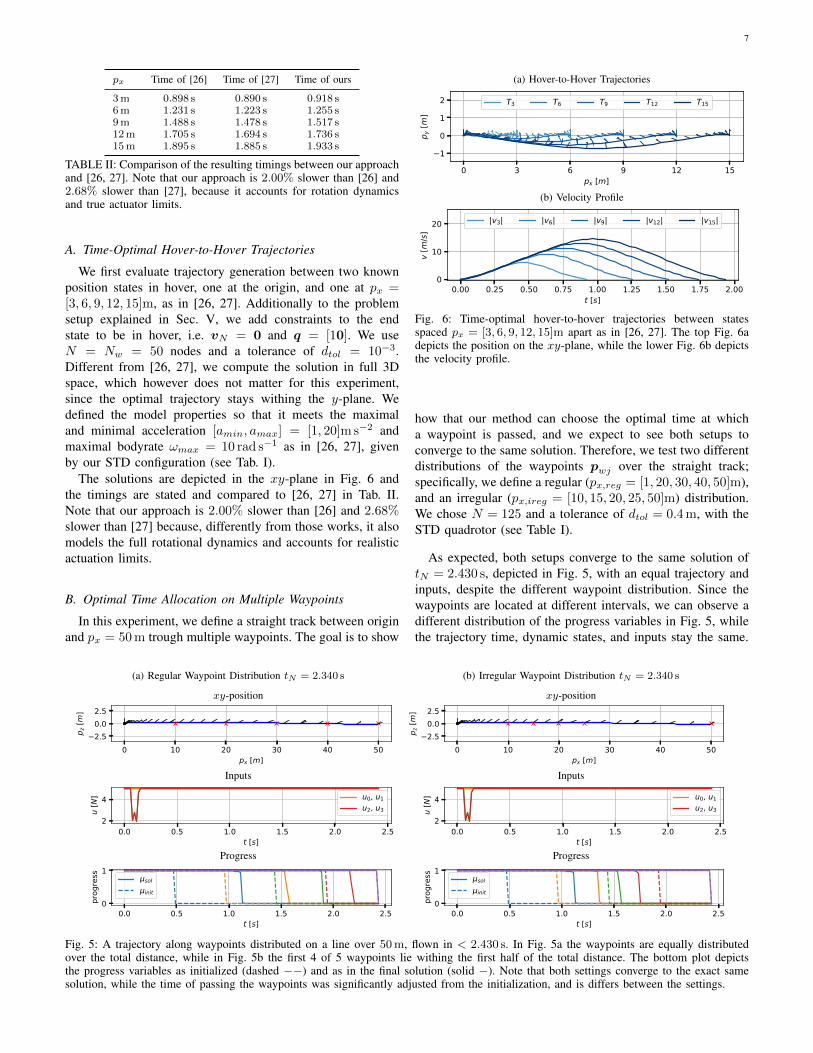
px Time of [26] Time of [27] Time of ours
3m 0.898 s 0.890 s 0.918 s6m 1.231 s 1.223 s 1.255 s9m 1.488 s 1.478 s 1.517 s12m 1.705 s 1.694 s 1.736 s15m 1.895 s 1.885 s 1.933 s
TABLE II: Comparison of the resulting timings between our approachand [26, 27]. Note that our approach is 2.00% slower than [26] and2.68% slower than [27], because it accounts for rotation dynamicsand true actuator limits.
A. Time-Optimal Hover-to-Hover Trajectories
We first evaluate trajectory generation between two knownposition states in hover, one at the origin, and one at px =[3, 6, 9, 12, 15]m, as in [26, 27]. Additionally to the problemsetup explained in Sec. V, we add constraints to the endstate to be in hover, i.e. vN = 0 and q = [10]. We useN = Nw = 50 nodes and a tolerance of dtol = 10−3.Different from [26, 27], we compute the solution in full 3Dspace, which however does not matter for this experiment,since the optimal trajectory stays withing the y-plane. Wedefined the model properties so that it meets the maximaland minimal acceleration [amin, amax] = [1, 20]m s−2 andmaximal bodyrate ωmax = 10 rad s−1 as in [26, 27], givenby our STD configuration (see Tab. I).
The solutions are depicted in the xy-plane in Fig. 6 andthe timings are stated and compared to [26, 27] in Tab. II.Note that our approach is 2.00% slower than [26] and 2.68%slower than [27] because, differently from those works, it alsomodels the full rotational dynamics and accounts for realisticactuation limits.
B. Optimal Time Allocation on Multiple Waypoints
In this experiment, we define a straight track between originand px = 50m trough multiple waypoints. The goal is to show
(a) Hover-to-Hover Trajectories
0 3 6 9 12 15px [m]
1
0
1
2
p y [m
]
T3 T6 T9 T12 T15
(b) Velocity Profile
0.00 0.25 0.50 0.75 1.00 1.25 1.50 1.75 2.00t [s]
0
10
20
v [m
/s]
|v3| |v6| |v9| |v12| |v15|
Fig. 6: Time-optimal hover-to-hover trajectories between statesspaced px = [3, 6, 9, 12, 15]m apart as in [26, 27]. The top Fig. 6adepicts the position on the xy-plane, while the lower Fig. 6b depictsthe velocity profile.
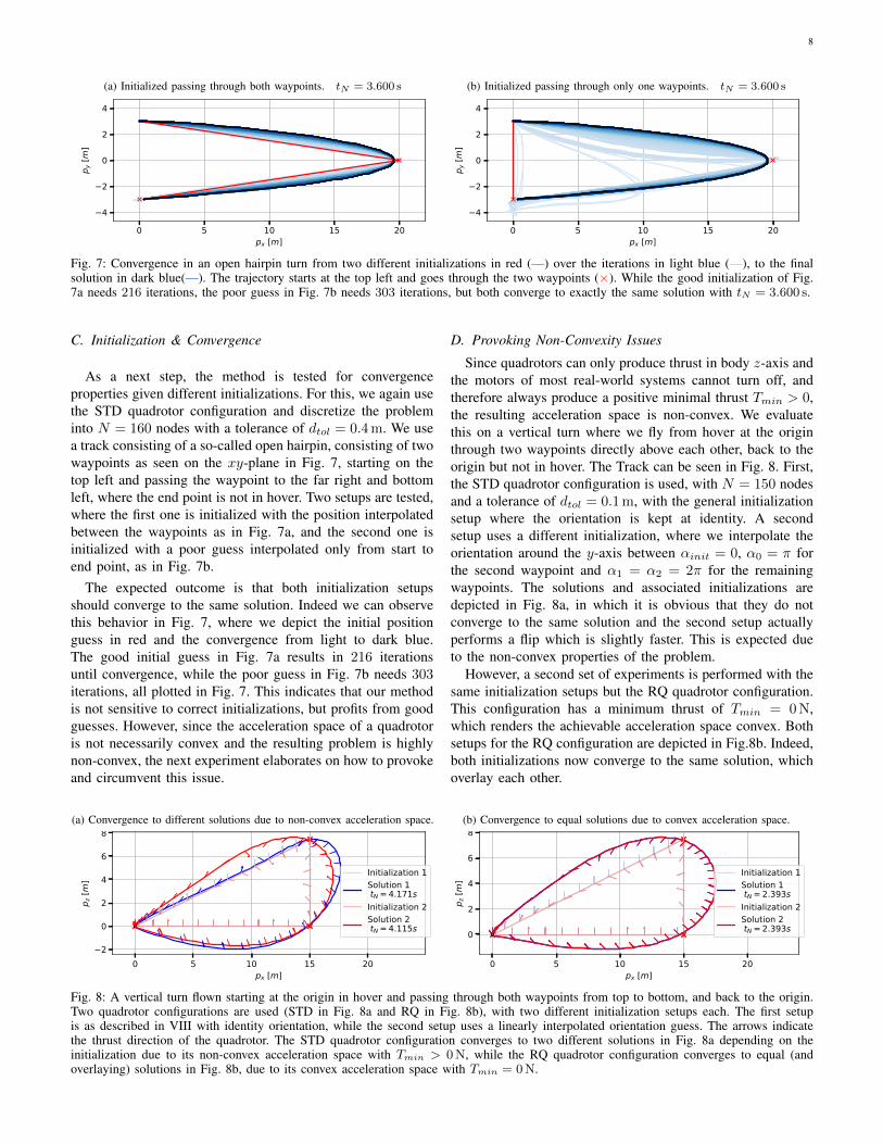
how that our method can choose the optimal time at whicha waypoint is passed, and we expect to see both setups toconverge to the same solution. Therefore, we test two differentdistributions of the waypoints pwj over the straight track;specifically, we define a regular (px,reg = [1, 20, 30, 40, 50]m),and an irregular (px,ireg = [10, 15, 20, 25, 50]m) distribution.We chose N = 125 and a tolerance of dtol = 0.4m, with theSTD quadrotor (see Table I).
As expected, both setups converge to the same solution oftN = 2.430 s, depicted in Fig. 5, with an equal trajectory andinputs, despite the different waypoint distribution. Since thewaypoints are located at different intervals, we can observe adifferent distribution of the progress variables in Fig. 5, whilethe trajectory time, dynamic states, and inputs stay the same.
(a) Regular Waypoint Distribution tN = 2.340 s
xy-position
0 10 20 30 40 50px [m]
2.50.02.5
p z [m
]
0.0 0.5 1.0 1.5 2.0 2.5t [s]
2
4
u [N
] u0, u1u2, u3
0.0 0.5 1.0 1.5 2.0 2.5t [s]
0
1
prog
ress
sol
init
Inputs0 10 20 30 40 50
px [m]
2.50.02.5
p z [m
]
0.0 0.5 1.0 1.5 2.0 2.5t [s]
2
4
u [N
] u0, u1u2, u3
0.0 0.5 1.0 1.5 2.0 2.5t [s]
0
1
prog
ress
sol
init
Progress
0 10 20 30 40 50px [m]
2.50.02.5
p z [m
]
0.0 0.5 1.0 1.5 2.0 2.5t [s]
2
4
u [N
] u0, u1u2, u3
0.0 0.5 1.0 1.5 2.0 2.5t [s]
0
1
prog
ress
sol
init
(b) Irregular Waypoint Distribution tN = 2.340 s
xy-position
0 10 20 30 40 50px [m]
2.50.02.5
p z [m
]
0.0 0.5 1.0 1.5 2.0 2.5t [s]
2
4
u [N
] u0, u1u2, u3
0.0 0.5 1.0 1.5 2.0 2.5t [s]
0
1
prog
ress
sol
init
Inputs0 10 20 30 40 50
px [m]
2.50.02.5
p z [m
]
0.0 0.5 1.0 1.5 2.0 2.5t [s]
2
4
u [N
] u0, u1u2, u3
0.0 0.5 1.0 1.5 2.0 2.5t [s]
0
1
prog
ress
sol
init
Progress
0 10 20 30 40 50px [m]
2.50.02.5
p z [m
]
0.0 0.5 1.0 1.5 2.0 2.5t [s]
2
4
u [N
] u0, u1u2, u3
0.0 0.5 1.0 1.5 2.0 2.5t [s]
0
1
prog
ress
sol
init
Fig. 5: A trajectory along waypoints distributed on a line over 50m, flown in < 2.430 s. In Fig. 5a the waypoints are equally distributedover the total distance, while in Fig. 5b the first 4 of 5 waypoints lie withing the first half of the total distance. The bottom plot depictsthe progress variables as initialized (dashed −−) and as in the final solution (solid −). Note that both settings converge to the exact samesolution, while the time of passing the waypoints was significantly adjusted from the initialization, and is differs between the settings.
8
(a) Initialized passing through both waypoints. tN = 3.600 s
0 5 10 15 20px [m]
4
2
0
2
4
p y [m
]Good Initialization Guess Ttotal = 3.600s (b) Initialized passing through only one waypoints. tN = 3.600 s
0 5 10 15 20px [m]
4
2
0
2
4
p y [m
]
Poor Initialization Guess Ttotal = 3.600s
Fig. 7: Convergence in an open hairpin turn from two different initializations in red (—) over the iterations in light blue (—), to the finalsolution in dark blue(—). The trajectory starts at the top left and goes through the two waypoints (×). While the good initialization of Fig.7a needs 216 iterations, the poor guess in Fig. 7b needs 303 iterations, but both converge to exactly the same solution with tN = 3.600 s.
C. Initialization & Convergence
As a next step, the method is tested for convergenceproperties given different initializations. For this, we again usethe STD quadrotor configuration and discretize the probleminto N = 160 nodes with a tolerance of dtol = 0.4m. We usea track consisting of a so-called open hairpin, consisting of twowaypoints as seen on the xy-plane in Fig. 7, starting on thetop left and passing the waypoint to the far right and bottomleft, where the end point is not in hover. Two setups are tested,where the first one is initialized with the position interpolatedbetween the waypoints as in Fig. 7a, and the second one isinitialized with a poor guess interpolated only from start toend point, as in Fig. 7b.
The expected outcome is that both initialization setupsshould converge to the same solution. Indeed we can observethis behavior in Fig. 7, where we depict the initial positionguess in red and the convergence from light to dark blue.The good initial guess in Fig. 7a results in 216 iterationsuntil convergence, while the poor guess in Fig. 7b needs 303iterations, all plotted in Fig. 7. This indicates that our methodis not sensitive to correct initializations, but profits from goodguesses. However, since the acceleration space of a quadrotoris not necessarily convex and the resulting problem is highlynon-convex, the next experiment elaborates on how to provokeand circumvent this issue.
D. Provoking Non-Convexity Issues
Since quadrotors can only produce thrust in body z-axis andthe motors of most real-world systems cannot turn off, andtherefore always produce a positive minimal thrust Tmin > 0,the resulting acceleration space is non-convex. We evaluatethis on a vertical turn where we fly from hover at the originthrough two waypoints directly above each other, back to theorigin but not in hover. The Track can be seen in Fig. 8. First,the STD quadrotor configuration is used, with N = 150 nodesand a tolerance of dtol = 0.1m, with the general initializationsetup where the orientation is kept at identity. A secondsetup uses a different initialization, where we interpolate theorientation around the y-axis between αinit = 0, α0 = π forthe second waypoint and α1 = α2 = 2π for the remainingwaypoints. The solutions and associated initializations aredepicted in Fig. 8a, in which it is obvious that they do notconverge to the same solution and the second setup actuallyperforms a flip which is slightly faster. This is expected dueto the non-convex properties of the problem.
However, a second set of experiments is performed with thesame initialization setups but the RQ quadrotor configuration.This configuration has a minimum thrust of Tmin = 0N,which renders the achievable acceleration space convex. Bothsetups for the RQ configuration are depicted in Fig.8b. Indeed,both initializations now converge to the same solution, whichoverlay each other.
(a) Convergence to different solutions due to non-convex acceleration space.
Fig. 8: A vertical turn flown starting at the origin in hover and passing through both waypoints from top to bottom, and back to the origin.Two quadrotor configurations are used (STD in Fig. 8a and RQ in Fig. 8b), with two different initialization setups each. The first setupis as described in VIII with identity orientation, while the second setup uses a linearly interpolated orientation guess. The arrows indicatethe thrust direction of the quadrotor. The STD quadrotor configuration converges to two different solutions in Fig. 8a depending on theinitialization due to its non-convex acceleration space with Tmin > 0N, while the RQ quadrotor configuration converges to equal (andoverlaying) solutions in Fig. 8b, due to its convex acceleration space with Tmin = 0N.
9
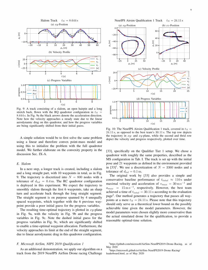
Slalom Track tN = 8.644 s
(a) xy-Position
20 10 0 10 20 30 40 50 60px [m]
10
0
p y [m
]
(b) Velocity Profile
0 2 4 6 8t [s]
25
0
25
v [m
/s] vx
vy
vz
|v|
(c) Progress Variables
0 2 4 6 8t [s]
0.0
0.5
1.0
prog
ress
init
sol
Fig. 9: A track consisting of a slalom, an open hairpin and a longstretch back, flown with the RQ quadrotor configuration in tN =8.644 s. In Fig. 9a the black arrows denote the acceleration direction.Note how the velocity approaches a steady state due to the linearaerodynamic drag on this quadrotor, and how the progress variablesare being significantly shifted from their initial guess.
A simple solution would be to first solve the same problemusing a linear and therefore convex point-mass model andusing this to initialize the problem with the full quadrotormodel. We further elaborate on the convexity property in thediscussion Sec. IX-A.
E. Slalom
In a next step, a longer track is created, including a slalomand a long straight part, with 10 waypoints in total, as in Fig.9. The trajectory is discretized into N = 800 nodes with atolerance of dtol = 0.4m. The RC quadrotor configurationis deployed in this experiment. We expect the trajectory tosmoothly slalom through the first 6 waypoints, take an sharpturn and accelerate back through the long straight segment.The straight segment is on purpose spanned by 4 unequallyspaced waypoints, which together with the 6 previous way-point provide a poor initial guess for the progress variables.
The resulting time-optimal trajectory is plotted in xy-planein Fig. 9a, with the velocity in Fig. 9b and the progressvariables in Fig. 9c. Note the dashed initial guess for theprogress variables in Fig. 9c, which are significantly shiftedto enable a time-optimal waypoint allocation. Furthermore, thevelocity approaches its limit at the end of the straight segment,due to linear aerodynamic drag in this quadrotor configuration.
F. Microsoft AirSim, NIPS 2019 Qualification 1
As an additional demonstration, we apply our algorithm on atrack from the 2019 NeurIPS AirSim Drone racing Challenge
NeurIPS Airsim Qualification 1 Track tN = 24.11 s
(a) xy-Position
25 0 25 50px [m]
80
60
40
20
0
p y [m
]
(b) xz-Position
20 0 20 40px [m]
0
20
40
60
p z [m
]
(c) Velocity Profile
0 5 10 15 20 25t [s]
20
0
20
v [m
/s]
vx
vy
vz
|v|
(d) Progress Variables
0 5 10 15 20 25t [s]
0.0
0.5
1.0
prog
ress
Fig. 10: The NeurIPS Airsim Qualification 1 track, covered in tN =24.11 s, as opposed to the best team’s 30.11 s. The top row depictsthe trajectory in xy- and xy-plane, while the second and thrid rowdepict the velocity and progress respectively, plotted over time.
[33], specifically on the Qualifier Tier 1 setup. We chose aquadrotor with roughly the same properties, described as theMS configuration in Tab. I. The track is set up with the initialpose and 21 waypoints as defined in the environment providedin [33]1. We use a discretization of N = 3360 nodes and atolerance of dtol = 0.1m.
The original work by [33] also provides a simple andconservative baseline performance of ttotal ≈ 110 s undermaximal velocity and acceleration of vmax = 30m s−1 andamax = 15m s−1, respectively. However, the best teamachieved a time of ttotal = 30.11 s according to the evaluationpage2. Our method generates a trajectory that passes all way-points at a mere tN = 24.11 s. Please note that this trajectoryshould only serve as a theoretical lower bound on the possiblyachievable time given the model parameters. However, themodel parameters were chosen slightly more conservative thanthe actual simulated drone for the qualification, to provide areasonable optimal-time solution.
1https://github.com/microsoft/AirSim-NeurIPS2019-Drone-Racing, as ofMay 2020
2https://microsoft.github.io/AirSim-NeurIPS2019-Drone-Racing/leaderboard.html, as of May 2020
10
25 20 15 10 5 0 5 10 15 20 25px [m]
10
5
0
5
10
15
p y [m
]Huma vs. Time-Optimal Trajectory
human tN = 10.338soptimal tN = 9.621s
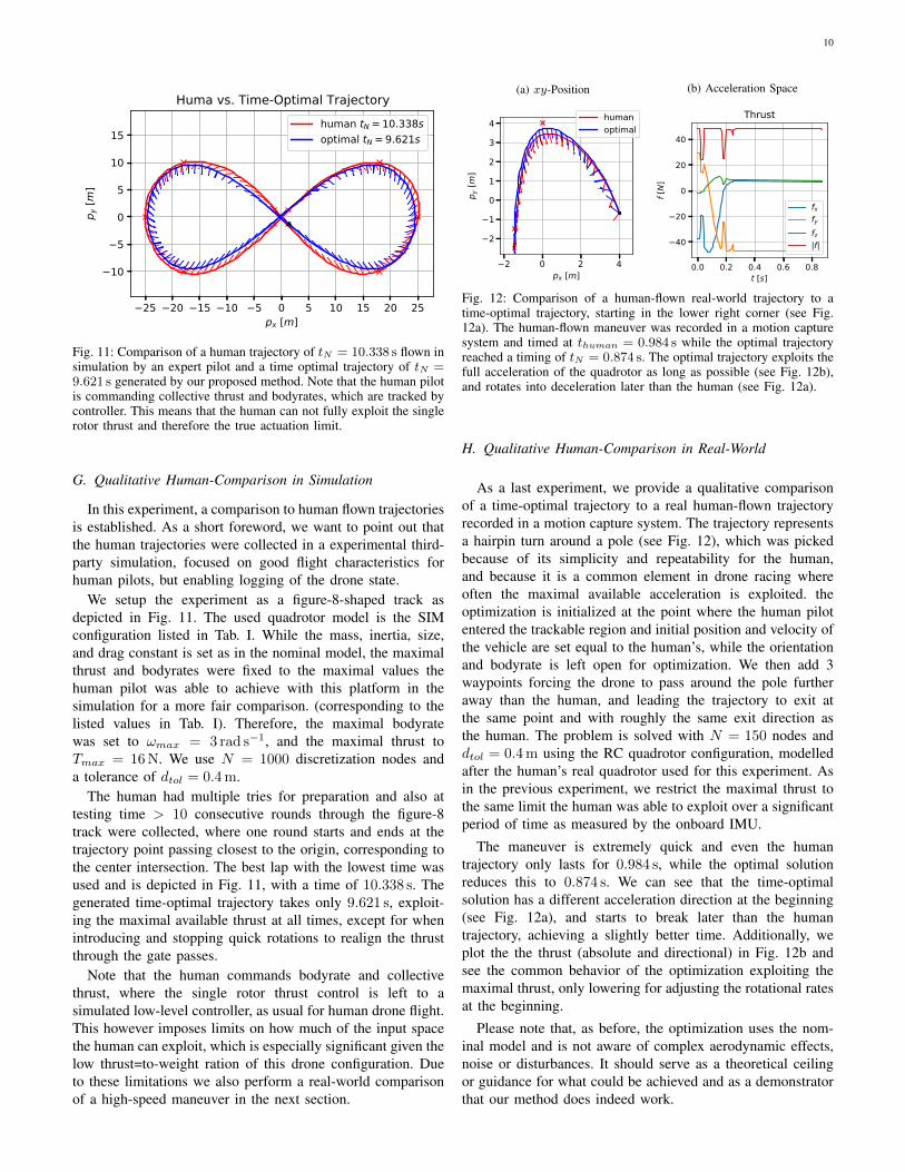
Fig. 11: Comparison of a human trajectory of tN = 10.338 s flown insimulation by an expert pilot and a time optimal trajectory of tN =9.621 s generated by our proposed method. Note that the human pilotis commanding collective thrust and bodyrates, which are tracked bycontroller. This means that the human can not fully exploit the singlerotor thrust and therefore the true actuation limit.
G. Qualitative Human-Comparison in Simulation
In this experiment, a comparison to human flown trajectoriesis established. As a short foreword, we want to point out thatthe human trajectories were collected in a experimental third-party simulation, focused on good flight characteristics forhuman pilots, but enabling logging of the drone state.
We setup the experiment as a figure-8-shaped track asdepicted in Fig. 11. The used quadrotor model is the SIMconfiguration listed in Tab. I. While the mass, inertia, size,and drag constant is set as in the nominal model, the maximalthrust and bodyrates were fixed to the maximal values thehuman pilot was able to achieve with this platform in thesimulation for a more fair comparison. (corresponding to thelisted values in Tab. I). Therefore, the maximal bodyratewas set to ωmax = 3 rad s−1, and the maximal thrust toTmax = 16N. We use N = 1000 discretization nodes anda tolerance of dtol = 0.4m.
The human had multiple tries for preparation and also attesting time > 10 consecutive rounds through the figure-8track were collected, where one round starts and ends at thetrajectory point passing closest to the origin, corresponding tothe center intersection. The best lap with the lowest time wasused and is depicted in Fig. 11, with a time of 10.338 s. Thegenerated time-optimal trajectory takes only 9.621 s, exploit-ing the maximal available thrust at all times, except for whenintroducing and stopping quick rotations to realign the thrustthrough the gate passes.
Note that the human commands bodyrate and collectivethrust, where the single rotor thrust control is left to asimulated low-level controller, as usual for human drone flight.This however imposes limits on how much of the input spacethe human can exploit, which is especially significant given thelow thrust=to-weight ration of this drone configuration. Dueto these limitations we also perform a real-world comparisonof a high-speed maneuver in the next section.
(a) xy-Position
2 0 2 4px [m]
2
1
0
1
2
3
4
p y [m
]
humanoptimal
(b) Acceleration Space
0.0 0.2 0.4 0.6 0.8t [s]
40
20
0
20
40
f [N
]
Thrust
fxfyfz|f|
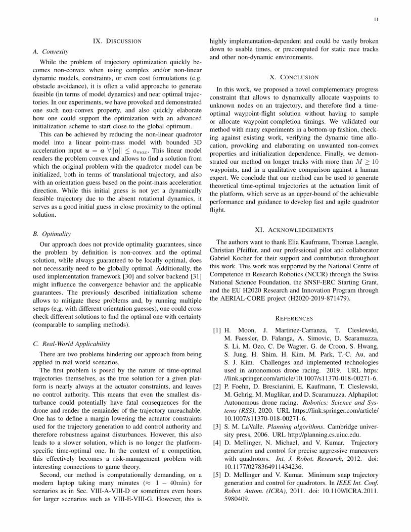
Fig. 12: Comparison of a human-flown real-world trajectory to atime-optimal trajectory, starting in the lower right corner (see Fig.12a). The human-flown maneuver was recorded in a motion capturesystem and timed at thuman = 0.984 s while the optimal trajectoryreached a timing of tN = 0.874 s. The optimal trajectory exploits thefull acceleration of the quadrotor as long as possible (see Fig. 12b),and rotates into deceleration later than the human (see Fig. 12a).
H. Qualitative Human-Comparison in Real-World
As a last experiment, we provide a qualitative comparisonof a time-optimal trajectory to a real human-flown trajectoryrecorded in a motion capture system. The trajectory representsa hairpin turn around a pole (see Fig. 12), which was pickedbecause of its simplicity and repeatability for the human,and because it is a common element in drone racing whereoften the maximal available acceleration is exploited. theoptimization is initialized at the point where the human pilotentered the trackable region and initial position and velocity ofthe vehicle are set equal to the human’s, while the orientationand bodyrate is left open for optimization. We then add 3waypoints forcing the drone to pass around the pole furtheraway than the human, and leading the trajectory to exit atthe same point and with roughly the same exit direction asthe human. The problem is solved with N = 150 nodes anddtol = 0.4m using the RC quadrotor configuration, modelledafter the human’s real quadrotor used for this experiment. Asin the previous experiment, we restrict the maximal thrust tothe same limit the human was able to exploit over a significantperiod of time as measured by the onboard IMU.
The maneuver is extremely quick and even the humantrajectory only lasts for 0.984 s, while the optimal solutionreduces this to 0.874 s. We can see that the time-optimalsolution has a different acceleration direction at the beginning(see Fig. 12a), and starts to break later than the humantrajectory, achieving a slightly better time. Additionally, weplot the the thrust (absolute and directional) in Fig. 12b andsee the common behavior of the optimization exploiting themaximal thrust, only lowering for adjusting the rotational ratesat the beginning.
Please note that, as before, the optimization uses the nom-inal model and is not aware of complex aerodynamic effects,noise or disturbances. It should serve as a theoretical ceilingor guidance for what could be achieved and as a demonstratorthat our method does indeed work.
11
IX. DISCUSSION
A. Convexity
While the problem of trajectory optimization quickly be-comes non-convex when using complex and/or non-lineardynamic models, constraints, or even cost formulations (e.g.obstacle avoidance), it is often a valid approache to generatefeasible (in terms of model dynamics) and near optimal trajec-tories. In our experiments, we have provoked and demonstratedone such non-convex property, and also quickly elaboratehow one could support the optimization with an advancedinitialization scheme to start close to the global optimum.
This can be achieved by reducing the non-linear quadrotormodel into a linear point-mass model with bounded 3Dacceleration input u = a ∀‖a‖ ≤ amax. This linear modelrenders the problem convex and allows to find a solution fromwhich the original problem with the quadrotor model can beinitialized, both in terms of translational trajectory, and alsowith an orientation guess based on the point-mass accelerationdirection. While this initial guess is not yet a dynamicallyfeasible trajectory due to the absent rotational dynamics, itserves as a good initial guess in close proximity to the optimalsolution.
B. Optimality
Our approach does not provide optimality guarantees, sincethe problem by definition is non-convex and the optimalsolution, while always guaranteed to be locally optimal, doesnot necessarily need to be globally optimal. Additionally, theused implementation framework [30] and solver backend [31]might influence the convergence behavior and the applicableguarantees. The previously described initialization schemeallows to mitigate these problems and, by running multiplesetups (e.g. with different orientation guesses), one could crosscheck different solutions to find the optimal one with certainty(comparable to sampling methods).
C. Real-World Applicability
There are two problems hindering our approach from beingapplied in real world scenarios.
The first problem is posed by the nature of time-optimaltrajectories themselves, as the true solution for a given plat-form is nearly always at the actuator constraints, and leavesno control authority. This means that even the smallest dis-turbance could potentially have fatal consequences for thedrone and render the remainder of the trajectory unreachable.One has to define a margin lowering the actuator constraintsused for the trajectory generation to add control authority andtherefore robustness against disturbances. However, this alsoleads to a slower solution, which is no longer the platform-specific time-optimal one. In the context of a competition,this effectively becomes a risk-management problem withinteresting connections to game theory.
Second, our method is computationally demanding, on amodern laptop taking many minutes (≈ 1 − 40min) forscenarios as in Sec. VIII-A-VIII-D or sometimes even hoursfor larger scenarios such as VIII-E-VIII-G. However, this is
highly implementation-dependent and could be vastly brokendown to usable times, or precomputed for static race tracksand other non-dynamic environments.
X. CONCLUSION
In this work, we proposed a novel complementary progressconstraint that allows to dynamically allocate waypoints tounknown nodes on an trajectory, and therefore find a time-optimal waypoint-flight solution without having to sampleor allocate waypoint-completion timings. We validated ourmethod with many experiments in a bottom-up fashion, check-ing against existing work, verifying the dynamic time allo-cation, provoking and elaborating on unwanted non-convexproperties and initialization dependence. Finally, we demon-strated our method on longer tracks with more than M ≥ 10waypoints, and in a qualitative comparison against a humanexpert. We conclude that our method can be used to generatetheoretical time-optimal trajectories at the actuation limit ofthe platform, which serve as an upper-bound of the achievableperformance and guidance to develop fast and agile quadrotorflight.
XI. ACKNOWLEDGEMENTS
The authors want to thank Elia Kaufmann, Thomas Laengle,Christian Pfeiffer, and our professional pilot and collaboratorGabriel Kocher for their support and contribution throughoutthis work. This work was supported by the National Centre ofCompetence in Research Robotics (NCCR) through the SwissNational Science Foundation, the SNSF-ERC Starting Grant,and the EU H2020 Research and Innovation Program throughthe AERIAL-CORE project (H2020-2019-871479).
REFERENCES
[1] H. Moon, J. Martinez-Carranza, T. Cieslewski,M. Faessler, D. Falanga, A. Simovic, D. Scaramuzza,S. Li, M. Ozo, C. De Wagter, G. de Croon, S. Hwang,S. Jung, H. Shim, H. Kim, M. Park, T.-C. Au, andS. J. Kim. Challenges and implemented technologiesused in autonomous drone racing. 2019. URL https://link.springer.com/article/10.1007/s11370-018-00271-6.
[2] P. Foehn, D. Brescianini, E. Kaufmann, T. Cieslewski,M. Gehrig, M. Muglikar, and D. Scaramuzza. Alphapilot:Autonomous drone racing. Robotics: Science and Sys-tems (RSS), 2020. URL https://link.springer.com/article/10.1007/s11370-018-00271-6.
[3] S. M. LaValle. Planning algorithms. Cambridge univer-sity press, 2006. URL http://planning.cs.uiuc.edu.
[4] D. Mellinger, N. Michael, and V. Kumar. Trajectorygeneration and control for precise aggressive maneuverswith quadrotors. Int. J. Robot. Research, 2012. doi:10.1177/0278364911434236.
[5] D. Mellinger and V. Kumar. Minimum snap trajectorygeneration and control for quadrotors. In IEEE Int. Conf.Robot. Autom. (ICRA), 2011. doi: 10.1109/ICRA.2011.5980409.
12
[6] C. R. Hargraves and S. W. Paris. Direct trajectoryoptimization using nonlinear programming and colloca-tion. J. Guidance, Control, and Dynamics, 1987. doi:10.2514/3.20223.
[7] S. Bouabdallah and R. Siegwart. Full control of aquadrotor. In IEEE/RSJ Int. Conf. Intell. Robot. Syst.(IROS), 2007. doi: 10.1109/IROS.2007.4399042.
[8] R. Mahony, V. Kumar, and P. Corke. Multirotor aerialvehicles: Modeling, estimation, and control of quadrotor.IEEE Robot. Autom. Mag., 2012. doi: 10.1109/MRA.2012.2206474.
[9] M. Faessler, A. Franchi, and D. Scaramuzza. Differentialflatness of quadrotor dynamics subject to rotor dragfor accurate tracking of high-speed trajectories. IEEERobot. Autom. Lett., April 2018. doi: 10.1109/LRA.2017.2776353.
[10] T. Tomic, P. Lutz, K. Schmid, A. Mathers, and S. Had-dadin. Simultaneous contact and aerodynamic forceestimation (s-cafe) for aerial robots. Int. J. Robot.Research, 2020. doi: 10.1177/0278364920904788.
[11] M. Faessler, D. Falanga, and D. Scaramuzza. Thrustmixing, saturation, and body-rate control for accurateaggressive quadrotor flight. IEEE Robot. Autom. Lett.,April 2017. doi: 10.1109/LRA.2016.2640362.
[12] M. Bangura and R. Mahony. Real-time model predictivecontrol for quadrotors. IFAC World Congress, 2014. doi:10.3182/20140824-6-za-1003.00203.
[13] M. Neunert, C. de Crousaz, F. Furrer, M. Kamel,F. Farshidian, R. Siegwart, and J. Buchli. Fast nonlinearmodel predictive control for unified trajectory optimiza-tion and tracking. In IEEE Int. Conf. Robot. Autom.(ICRA), 2016. doi: 10.1109/icra.2016.7487274.
[14] D. Falanga, P. Foehn, P. Lu, and D. Scaramuzza.PAMPC: Perception-aware model predictive control forquadrotors. In IEEE/RSJ Int. Conf. Intell. Robot. Syst.(IROS), 2018.
[15] C. Richter, A. Bry, and N. Roy. Polynomial Tra-jectory Planning for Aggressive Quadrotor Flight inDense Indoor Environments. 2016. doi: 10.1007/978-3-319-28872-7-37.
[16] M. W. Mueller, M. Hehn, and R. D’Andrea. A computa-tionally efficient algorithm for state-to-state quadrocoptertrajectory generation and feasibility verification. InIEEE/RSJ Int. Conf. Intell. Robot. Syst. (IROS), 2013.doi: 10.1109/iros.2013.6696852.
[17] R. Allen and M. Pavone. A real-time framework for kino-dynamic planning with application to quadrotor obstacleavoidance. In AIAA Guidance, Navigation, and ControlConference, 2016. doi: 10.2514/6.2016-1374.
[18] N. Ratliff, M. Zucker, J A. Bagnell, and S. Srinivasa.CHOMP: Gradient optimization techniques for efficientmotion planning. In IEEE Int. Conf. Robot. Autom.(ICRA), 2009. doi: 10.1109/ROBOT.2009.5152817.
[19] M. Posa, S. Kuindersma, and R. Tedrake. Optimizationand stabilization of trajectories for constrained dynamicalsystems. In IEEE Int. Conf. Robot. Autom. (ICRA), 2016.
doi: 10.1109/ICRA.2016.7487270.[20] P. Foehn, D. Falanga, N. Kuppuswamy, R. Tedrake, and
D. Scaramuzza. Fast trajectory optimization for agilequadrotor maneuvers with a cable-suspended payload. InRobotics: Science and Systems (RSS), 2017.
[21] M. Diehl, H. G. Bock, H. Diedam, and P. B. Wieber.Fast direct multiple shooting algorithms for optimal robotcontrol. In Fast motions in biomechanics and robotics.Springer, 2006.
[22] M. Geisert and N. Mansard. Trajectory generation forquadrotor based systems using numerical optimal control.In IEEE Int. Conf. Robot. Autom. (ICRA), 2016. doi:10.1109/ICRA.2016.7487460.
[23] F. Augugliaro, A. P. Schoellig, and R. D’Andrea. Gen-eration of collision-free trajectories for a quadrocopterfleet: A sequential convex programming approach. InIEEE/RSJ Int. Conf. Intell. Robot. Syst. (IROS), 2012.doi: 10.1109/IROS.2012.6385823.
[24] S. Vakhrameev. A bang-bang theorem with a finite num-ber of switchings for nonlinear smooth control systems.J. Math. Sciences, June 1997. doi: 10.1007/BF02355111.
[25] L. Poggiolini and G. Stefani. Minimum time optimalityfor a bang-singular arc: Second order sufficient condi-tions. In IEEE Eur. Control Conf. (ECC), January 2006.doi: 10.1109/CDC.2005.1582360.
[26] M. Hehn, R. Ritz, and R. D’Andrea. Performancebenchmarking of quadrotor systems using time-optimalcontrol. Auton. Robots, March 2012. doi: 10.1007/s10514-012-9282-3.
[27] W. Van Loock, G. Pipeleers, and J. Swevers. Time-optimal quadrotor flight. In IEEE Eur. Control Conf.(ECC), 2013. doi: 10.23919/ECC.2013.6669253.
[28] S. Spedicato and G. Notarstefano. Minimum-time tra-jectory generation for quadrotors in constrained environ-ments. IEEE Transactions on Control Systems Technol-ogy, 2018. doi: 10.1109/TCST.2017.2709268.
[29] G. Ryou, E. Tal, and S. Karaman. Multi-fidelity black-box optimization for time-optimal quadrotor maneuvers.arXiv prepring: arXiv:2006.02513, June 2020. URLhttps://arxiv.org/abs/2006.02513.
[30] J. A. E. Andersson, J. Gillis, G. Horn, J. B. Rawlings,and M. Diehl. CasADi – A software framework for non-linear optimization and optimal control. MathematicalProgramming Computation, 2018.
[31] A. Wachter and L. Biegler. On the implementation of aninterior-point filter line-search algorithm for large-scalenonlinear programming. Mathematical programming,2006. doi: 10.1007/s10107-004-0559-y.
[32] S. Shah, D. Dey, C. Lovett, and A. Kapoor. Air-Sim: High-fidelity visual and physical simulation forautonomous vehicles. In Field and Service Robot., pages621–635, 2017.
[33] R. Madaan, N. Gyde, S. Vemprala, M. Brown,K. Nagami, T. Taubner, E. Cristofalo, D. Scaramuzza,M. Schwager, and A. Kapoor. Airsim drone racinglab. PMLR post-proceedings of the NeurIPS 2019’sCompetition Track, 2020.