7/27/2019 CPDRS1 - Solutions

http://slidepdf.com/reader/full/cpdrs1-solutions 1/7

 

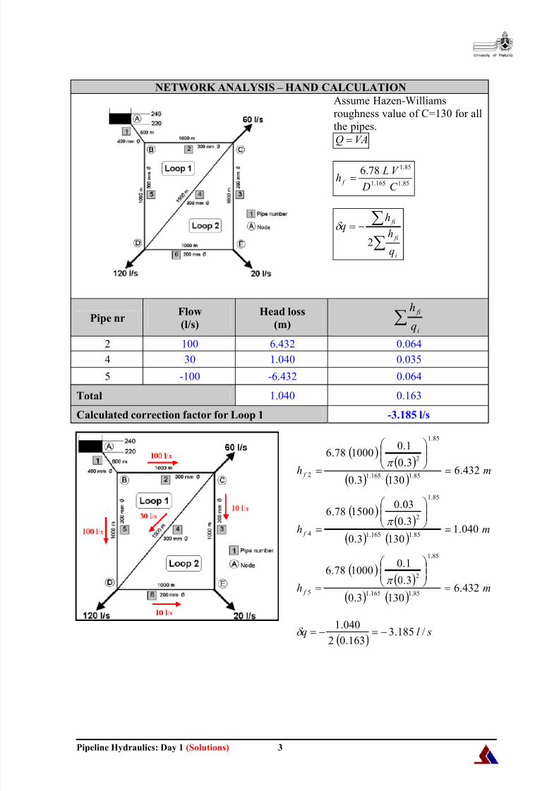
Pipeline Hydraulics: Day 1 (Solutions)  1

  PIPELINE DESIGN COURSE

DAY 1

PIPELINE HYDRAULICS

CONTINUING PROFESSIONAL DEVELOPMENT RESULTS SHEET

PIPELINE HYDRAULICS – HAND CALCULATION

Derive a relationship for the flowrate relationship for the threedifferent pipes.

Derive a relationship for therequired effective diameter toreplace the three parallel pipes.

Flow rate relationship

321   QQQQTotal    ++= ………………….(1)

321   f   f   f     hhh   ==   and VAQ =  

1

2

1111

2 gD

V  Lh f  

λ =   thus 

11

11

1

2

 L

h gDV 

  f  

λ = ………………….(2)

2

2

2222

2 gD

V  Lh f  

λ =   thus

22

22

2

2

 L

h gDV 

  f  

λ = ………………….(3)

3

2

3333

2 gD

V  Lh f  

λ =   thus

33

33

3

2

 L

h gDV 

  f  

λ = ………………….(4)

Substitute (2), (3) and (4) into (1)

 

  

 +

 

  

 +

 

  

 =

4

2

4

2

4

2 2

3

33

332

2

22

222

1

11

11   D

 L

h gD D

 L

h gD D

 L

h gDQ

  f   f   f  

Total 

π 

λ 

π 

λ 

π 

λ  

SOLUTIONS

7/27/2019 CPDRS1 - Solutions

http://slidepdf.com/reader/full/cpdrs1-solutions 2/7

 

Pipeline Hydraulics: Day 1 (Solutions)  2

 

PIPELINE HYDRAULICS – HAND CALCULATION

Effective diameter

321   f   f   f   fE    hhhh   ===  

3

2

333

2

2

222

1

2

111

2

2222   gD

V  L

 gD

V  L

 gD

V  L

 gD

V  L

 E 

 E  E  E    λ λ λ λ ===  

21

11

1

2

1  

  

 =

 E 

 E  E  E 

 D L

 DV  LV 

λ 

λ ………………….(1)

21

22

2

2

2  

  

 =

 E 

 E  E  E 

 D L

 DV  LV 

λ 

λ ………………….(2)

2

1

33

32

3  

  

 = E 

 E  E  E 

 D L

 DV  LV 

λ 

λ ………………….(3)

 E QQQQ   =++ 321  

 E  E  AV  AV  AV  AV    =++ 332211 ………………….(4)

Substitute (1), (2) and (3) into (4)

  

  =

  

  

  

  +

  

  

  

  +

  

  

  

  

4444

223

2

1

33

322

2

1

22

22

12

1

11

1   E  E 

 E 

 E  E  E 

 E 

 E  E  E 

 E 

 E  E  E 

 DV  D

 D L

 D LV  D

 D L

 D LV  D

 D L

 D LV    π π 

λ 

λ π 

λ 

λ π 

λ 

λ   

( ) ( ) ( ) 22

3

21

33

32

2

21

22

22

1

21

11

1 E 

 E 

 E  E 

 E 

 E  E 

 E 

 E  E   D D D L

 D L D

 D L

 D L D

 D L

 D L=

 

  

 +

 

  

 +

 

  

 

λ 

λ 

λ 

λ 

λ 

λ  

 

 

 

 

+

 

 

 

 

+

 

 

 

 

=33

2

5

3

22

2

5

2

11

2

5

12

5

 L

 D

 L

 D

 L

 D L D  E  E  E 

λ λ λ λ   

7/27/2019 CPDRS1 - Solutions

http://slidepdf.com/reader/full/cpdrs1-solutions 3/7

 

Pipeline Hydraulics: Day 1 (Solutions)  3

 

NETWORK ANALYSIS – HAND CALCULATION

Assume Hazen-Williamsroughness value of C=130 for allthe pipes.

VAQ =  

85.1165.1

85.178.6

C  D

V  Lh f    =  

∑

∑−=

i

 fi

 fi

q

h

hq

2

δ    

Pipe nrFlow

(l/s)

Head loss

(m) ∑i

 fi

q

h 

2 100 6.432 0.064

4 30 1.040 0.035

5 -100 -6.432 0.064

Total  1.040 0.163

Calculated correction factor for Loop 1 -3.185 l/s

( )( )

( ) ( )  mh f   432.6

1303.0

3.0

1.0100078.6

85.1165.1

85.1

2

2   = 

  

 

=  π 

( )( )

( ) ( )  mh f   040.1

1303.0

3.0

03.0150078.6

85.1165.1

85.1

2

4   = 

  

 

=  π 

( )( )

( ) ( )  mh f   432.6

1303.0

3.0

1.0100078.6

85.1165.1

85.1

2

5   = 

  

 

=  π 

( )  sl q /185.3

163.02

040.1−=−=δ  

7/27/2019 CPDRS1 - Solutions

http://slidepdf.com/reader/full/cpdrs1-solutions 4/7

 

Pipeline Hydraulics: Day 1 (Solutions)  4

 

ECONOMIC ANALYSIS – HAND CALCULATION

1. Evaluate which of the future income streams S1 or S2 is more favourable if the costof capital is 10% on a yearly basis.

2. Determine the current investment that should be made for the replacement of a R1.5mil installation (current cost) after 15 years, if the expected CPIX is 15 % and thereturn on a fixed investment is 8% pa.

3. Determine the Internal Rate of Return (IRR) for the following cash flow.

Question 1 

If you assume year 1 to be the base year than the NPV of the two income streams are: NPVS1 = R1 412.39 NPVS2 = R1 374.43

Resulting in income stream S1 being the most favourable when comparing the Net PresentValues (NPV).

This was calculated using the following formula:

( )n

i

 F  NPV 

+

=

1

 

Where:F = future valuei = interest raten = periodsEach future value was brought back to present values and accumulated to obtain the total

 NPV for each income stream 

Year S1 S21 250 100

2 350 400

3 600 350

4 100 600

5 400 250

Year Cash flow

0 -1300

1 250

2 350

3 600

4 100

5 400

7/27/2019 CPDRS1 - Solutions

http://slidepdf.com/reader/full/cpdrs1-solutions 5/7

 

Pipeline Hydraulics: Day 1 (Solutions)  5

 

ECONOMIC ANALYSIS – HAND CALCULATION

Question 2

First the future value of the investment should be determined. The current installation isworth R1 500 000 and the escalation will be 15 % for a 15 year period

( )ni P  F    += 1   ( ) 592205R1215.01000500115

=+= F   

 Now the current investment should be calculated by discounting the future required valuewith 8% per annum for the 15 year period.

( )ni

 F  P 

+=

1 

( )712847R3

08.01

5922051215  =

+= P   

Question 3

The internal rate of return is the rate where the NPVincome = NPVexpenditure 

( ) ( ) ( ) ( ) ( )543211

400

1

100

1

600

1

350

1

250

iiiii NPV income

++

++

++

++

+= ………………….(1)

( )0exp1

1300

i NPV  enditure

+= ………………….(2)

Equation (1) = Equation (2)

( ) ( ) ( ) ( ) ( ) ( )0543211

1300

1

400

1

100

1

600

1

350

1

250

iiiiii   +=

++

++

++

++

+ 

Solving from this equation for “i”

IRR = 9.525% 

7/27/2019 CPDRS1 - Solutions

http://slidepdf.com/reader/full/cpdrs1-solutions 6/7

 

Pipeline Hydraulics: Day 1 (Solutions)  6

 

Question Description Solution

NETWORK ANALYSES - PRACTICAL

D1Q1 Which nodes in the New York tunnel systemdo not adhere to the minimum pressure

requirement?

 Node 16 (64.47 m) Node 17 (80.90 m)

 Node 18 (48.35 m) Node 19 (30.10 m) Node 20 (64.05 m) 

D1Q2 What is the pressure drop in pipe 14 ? ∆h = 2.45 m (difference between pressures of node15 and 14)

D1Q3 What would the corresponding friction factor(λ ) in pipe 14 be, as used in the DarcyWeisbach equation?

λ  = 0.0192

D1Q4 If you had to add any parallel pipes to thesystem, where would you place these and why?

(Engineering gut feel)

Adding pipes close to thesupply reservoir usually

improves the pressure in theentire network. Anotheroption is to place parallel pipes along side pipes whichhave high unit head lossvalues such as pipes 17, 18,19 and 21. 

OPTIMIZATION - PRACTICAL

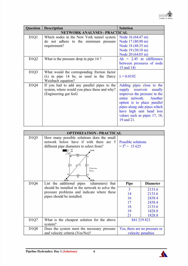
D1Q5 How many possible solutions does the smallnetwork below have if with there are 5different pipe diameters to select from?

Possible solutions= 56 = 15 625 

Pipe DiameterD1Q6 List the additional pipes (diameters) that

should be installed in the network to solve the pressure problems and indicate where these pipes should be installed.

3141617181921

2133.62133.62438.42438.42133.61828.81828.8

D1Q7 What is the cheapest solution for the abovesystem?

$41 219 821

D1Q8 Does the system meet the necessary pressure

and velocity criteria (Yes/No)?

Yes, there are no pressure or

velocity penalties

7/27/2019 CPDRS1 - Solutions

http://slidepdf.com/reader/full/cpdrs1-solutions 7/7

 

Pipeline Hydraulics: Day 1 (Solutions)  7

 

Question Description Solution

LIFE CYCLE COSTING ANALYSIS - PRACTICAL

D1Q9 What is the maximum flow rate for

Alternative 1 at the end of the design life(Ml/day)?

10.263 Ml/day in year 2019

D1Q10 What and where is the lowest pressure (m) inthe pipeline (year 1) for alternative 1? At chainage 1650 m the

 pressure is 4.115 m

D1Q11 What is the capital cost of Alternative 2?Total capital cost =R5 079 261

D1Q12 What is the IRR of Alternative 2?IRR = 62.511 %

D1Q13 What is the annual operating cost in year 15for alternative 2? Total operation cost =

R291 374.30

D1Q14 Which alternative would you recommend andwhy?

Alternative 1 cannot providethe total demand of 10.345Ml/day in year 2019 whilstAlternative 2 still has somespare capacity. The totalcapital cost of Alternative 1is however less than that ofAlternative 2 by ±R363 000.The IRR of alternative 1 isalso higher than that ofAlternative 2.

D1Q15 What other options do you have that willimprove the system, providing you with a

 better alternative?

Use pipes with less internalfriction.

Other pipe materials.Obtain the best combinationas shown in Alternative 2.Could add a booster pump.Different route.Provide greater headdifference between thereservoirs by lifting thesupply level or lowering theend reservoir level.

The two entered alternatives are provided electronically on the website:

Practical Example (Gravity system – Alternative 1).lccPractical Example (Gravity system – Alternative 2).lcc