148
CppSim Reference Manual Version 5 Michael H. Perrott http://www.cppsim.com Copyright c 2002-2011 by Michael H. Perrott All rights reserved
| Date post: | 20-Apr-2017 |
| Category: |
Documents |
| Upload: | samir-ahmed |
| View: | 219 times |
| Download: | 0 times |

CppSim Reference Manual
Version 5
Michael H. Perrott
http://www.cppsim.com
Copyright c© 2002-2011 by Michael H. Perrott
All rights reserved

2

3
He had no beauty or majesty to
attract us to him,
nothing in his appearance
that we should desire
him.
But he was pierced for our
transgressions,
he was crushed for our
iniquities;
the punishment that brought us
peace was upon him,
and by his wounds we are
healed.
Isaiah 53:2,5

4

Contents
1 Foreword 9
2 Introduction 11
2.1 Comparison to Other Simulation Packages . . . . . . . . . . . . . . . . . . . 11
2.2 Object Oriented Simulation Code . . . . . . . . . . . . . . . . . . . . . . . . 14
2.3 The Issue of Ordering . . . . . . . . . . . . . . . . . . . . . . . . . . . . . . . 16
2.4 Outline of Book . . . . . . . . . . . . . . . . . . . . . . . . . . . . . . . . . . 17
3 Setup and Use (Windows version) 19
3.1 Installation . . . . . . . . . . . . . . . . . . . . . . . . . . . . . . . . . . . . 19
3.2 Running CppSim . . . . . . . . . . . . . . . . . . . . . . . . . . . . . . . . . 20
3.3 CppSimShared Directory Contents . . . . . . . . . . . . . . . . . . . . . . . 21
4 Overview 23
4.1 Schematic Views . . . . . . . . . . . . . . . . . . . . . . . . . . . . . . . . . 23
4.2 Netlist Format (netlist) . . . . . . . . . . . . . . . . . . . . . . . . . . . . . . 25
4.3 Module Description File . . . . . . . . . . . . . . . . . . . . . . . . . . . . . 27
4.4 Simulation Description File (test.par) . . . . . . . . . . . . . . . . . . . . . . 30
4.5 CppSim Commands . . . . . . . . . . . . . . . . . . . . . . . . . . . . . . . . 30
4.6 Viewing Results . . . . . . . . . . . . . . . . . . . . . . . . . . . . . . . . . . 31
5 Specifying Simulation Parameters (test.par) 33
5.1 Parsing Rules . . . . . . . . . . . . . . . . . . . . . . . . . . . . . . . . . . . 33
5.2 num sim steps: . . . . . . . . . . . . . . . . . . . . . . . . . . . . . . . . . . 34
5.3 Ts: . . . . . . . . . . . . . . . . . . . . . . . . . . . . . . . . . . . . . . . . . 34
5.4 output: . . . . . . . . . . . . . . . . . . . . . . . . . . . . . . . . . . . . . . . 34
5.5 probe: . . . . . . . . . . . . . . . . . . . . . . . . . . . . . . . . . . . . . . . 37
5

6 CONTENTS
5.6 probe64: . . . . . . . . . . . . . . . . . . . . . . . . . . . . . . . . . . . . . . 38
5.7 global nodes: . . . . . . . . . . . . . . . . . . . . . . . . . . . . . . . . . . . 38
5.8 global param: . . . . . . . . . . . . . . . . . . . . . . . . . . . . . . . . . . . 38
5.9 top param: . . . . . . . . . . . . . . . . . . . . . . . . . . . . . . . . . . . . . 39
5.10 alter: . . . . . . . . . . . . . . . . . . . . . . . . . . . . . . . . . . . . . . . . 39
5.11 inp timing: . . . . . . . . . . . . . . . . . . . . . . . . . . . . . . . . . . . . . 40
5.12 inp dig: . . . . . . . . . . . . . . . . . . . . . . . . . . . . . . . . . . . . . . 41
5.13 mex prototype: . . . . . . . . . . . . . . . . . . . . . . . . . . . . . . . . . . 41
5.14 simulink prototype: . . . . . . . . . . . . . . . . . . . . . . . . . . . . . . . . 45
5.15 add top verilog libary file statements: . . . . . . . . . . . . . . . . . . . . . . 46
5.16 add bottom verilog libary file statements: . . . . . . . . . . . . . . . . . . . 46
5.17 add verilog test file statements: . . . . . . . . . . . . . . . . . . . . . . . . . 46
5.18 add verilog test module statements: . . . . . . . . . . . . . . . . . . . . . . . 47
5.19 ignore nodes output check: . . . . . . . . . . . . . . . . . . . . . . . . . . . . 48
5.20 allow verilog output clashing: . . . . . . . . . . . . . . . . . . . . . . . . . . 48
5.21 allow non bool signals in bus: . . . . . . . . . . . . . . . . . . . . . . . . . . 48
5.22 electrical integration damping factor: . . . . . . . . . . . . . . . . . . . . . . 48
5.23 temperature celsius for noise calc: . . . . . . . . . . . . . . . . . . . . . . . . 49
6 Writing Code for Primitives 51
6.1 Parsing Rules . . . . . . . . . . . . . . . . . . . . . . . . . . . . . . . . . . . 51
6.2 module: . . . . . . . . . . . . . . . . . . . . . . . . . . . . . . . . . . . . . . 52
6.3 description: . . . . . . . . . . . . . . . . . . . . . . . . . . . . . . . . . . . . 53
6.4 label as usrp module: . . . . . . . . . . . . . . . . . . . . . . . . . . . . . . . 53
6.5 parameters: . . . . . . . . . . . . . . . . . . . . . . . . . . . . . . . . . . . . 53
6.6 inputs: . . . . . . . . . . . . . . . . . . . . . . . . . . . . . . . . . . . . . . . 54
6.7 outputs: . . . . . . . . . . . . . . . . . . . . . . . . . . . . . . . . . . . . . . 54
6.8 classes: . . . . . . . . . . . . . . . . . . . . . . . . . . . . . . . . . . . . . . . 54
6.9 static variables: . . . . . . . . . . . . . . . . . . . . . . . . . . . . . . . . . . 55
6.10 set output vector lengths: . . . . . . . . . . . . . . . . . . . . . . . . . . . . 55
6.11 init: . . . . . . . . . . . . . . . . . . . . . . . . . . . . . . . . . . . . . . . . 56
6.12 end: . . . . . . . . . . . . . . . . . . . . . . . . . . . . . . . . . . . . . . . . 56
6.13 code: . . . . . . . . . . . . . . . . . . . . . . . . . . . . . . . . . . . . . . . . 57
6.14 electrical element: . . . . . . . . . . . . . . . . . . . . . . . . . . . . . . . . . 58
6.15 functions: . . . . . . . . . . . . . . . . . . . . . . . . . . . . . . . . . . . . . 60
CONTENTS 7
6.16 custom classes definition: and custom classes code: . . . . . . . . . . . . . . 61
6.17 sim order: . . . . . . . . . . . . . . . . . . . . . . . . . . . . . . . . . . . . . 62
6.18 stop current alter run . . . . . . . . . . . . . . . . . . . . . . . . . . . . . . . 63
6.19 timing sensitivity: . . . . . . . . . . . . . . . . . . . . . . . . . . . . . . . . . 64
7 General Purpose CppSim Classes 67
7.1 Vector and IntVector . . . . . . . . . . . . . . . . . . . . . . . . . . . . . . . 68
7.2 Matrix and IntMatrix . . . . . . . . . . . . . . . . . . . . . . . . . . . . . . . 75
7.3 List . . . . . . . . . . . . . . . . . . . . . . . . . . . . . . . . . . . . . . . . . 82
7.4 Clist . . . . . . . . . . . . . . . . . . . . . . . . . . . . . . . . . . . . . . . . 85
7.5 Probe . . . . . . . . . . . . . . . . . . . . . . . . . . . . . . . . . . . . . . . 89
7.6 Probe64 . . . . . . . . . . . . . . . . . . . . . . . . . . . . . . . . . . . . . . 91
7.7 Filter . . . . . . . . . . . . . . . . . . . . . . . . . . . . . . . . . . . . . . . . 93
7.8 Amp . . . . . . . . . . . . . . . . . . . . . . . . . . . . . . . . . . . . . . . . 97
7.9 EdgeDetect . . . . . . . . . . . . . . . . . . . . . . . . . . . . . . . . . . . . 99
7.10 SdMbitMod . . . . . . . . . . . . . . . . . . . . . . . . . . . . . . . . . . . . 101
7.11 Rand . . . . . . . . . . . . . . . . . . . . . . . . . . . . . . . . . . . . . . . . 103
7.12 OneOverfPlusWhiteNoise . . . . . . . . . . . . . . . . . . . . . . . . . . . . . 105
7.13 Quantizer . . . . . . . . . . . . . . . . . . . . . . . . . . . . . . . . . . . . . 106
8 CppSim Classes for PLL/DLL Simulation 111
8.1 SigGen . . . . . . . . . . . . . . . . . . . . . . . . . . . . . . . . . . . . . . . 112
8.2 Vco . . . . . . . . . . . . . . . . . . . . . . . . . . . . . . . . . . . . . . . . . 115
8.3 Delay . . . . . . . . . . . . . . . . . . . . . . . . . . . . . . . . . . . . . . . . 117
8.4 Divider . . . . . . . . . . . . . . . . . . . . . . . . . . . . . . . . . . . . . . . 118
8.5 Latch . . . . . . . . . . . . . . . . . . . . . . . . . . . . . . . . . . . . . . . . 119
8.6 Reg . . . . . . . . . . . . . . . . . . . . . . . . . . . . . . . . . . . . . . . . . 121
8.7 Xor . . . . . . . . . . . . . . . . . . . . . . . . . . . . . . . . . . . . . . . . . 123
8.8 And . . . . . . . . . . . . . . . . . . . . . . . . . . . . . . . . . . . . . . . . 125
8.9 Or . . . . . . . . . . . . . . . . . . . . . . . . . . . . . . . . . . . . . . . . . 127
8.10 EdgeMeasure . . . . . . . . . . . . . . . . . . . . . . . . . . . . . . . . . . . 129
A Example Simulation Code (Not Auto-Generated) 131
A.1 Classical Synthesizer . . . . . . . . . . . . . . . . . . . . . . . . . . . . . . . 132
A.2 Σ-Δ Synthesizer . . . . . . . . . . . . . . . . . . . . . . . . . . . . . . . . . . 135
8 CONTENTS
A.3 Linear CDR . . . . . . . . . . . . . . . . . . . . . . . . . . . . . . . . . . . . 137
A.4 Bang-bang CDR . . . . . . . . . . . . . . . . . . . . . . . . . . . . . . . . . 141
B Hspice Toolbox for Matlab 145
B.1 Setup . . . . . . . . . . . . . . . . . . . . . . . . . . . . . . . . . . . . . . . . 145
B.2 List of Functions . . . . . . . . . . . . . . . . . . . . . . . . . . . . . . . . . 146
B.3 Examples . . . . . . . . . . . . . . . . . . . . . . . . . . . . . . . . . . . . . 147
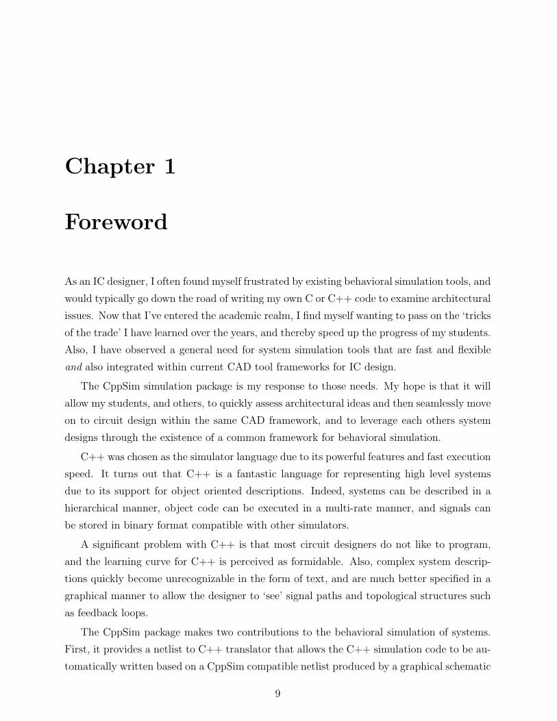
Chapter 1
Foreword
As an IC designer, I often found myself frustrated by existing behavioral simulation tools, and
would typically go down the road of writing my own C or C++ code to examine architectural
issues. Now that I’ve entered the academic realm, I find myself wanting to pass on the ‘tricks
of the trade’ I have learned over the years, and thereby speed up the progress of my students.
Also, I have observed a general need for system simulation tools that are fast and flexible
and also integrated within current CAD tool frameworks for IC design.
The CppSim simulation package is my response to those needs. My hope is that it will
allow my students, and others, to quickly assess architectural ideas and then seamlessly move
on to circuit design within the same CAD framework, and to leverage each others system
designs through the existence of a common framework for behavioral simulation.
C++ was chosen as the simulator language due to its powerful features and fast execution
speed. It turns out that C++ is a fantastic language for representing high level systems
due to its support for object oriented descriptions. Indeed, systems can be described in a
hierarchical manner, object code can be executed in a multi-rate manner, and signals can
be stored in binary format compatible with other simulators.
A significant problem with C++ is that most circuit designers do not like to program,
and the learning curve for C++ is perceived as formidable. Also, complex system descrip-
tions quickly become unrecognizable in the form of text, and are much better specified in a
graphical manner to allow the designer to ‘see’ signal paths and topological structures such
as feedback loops.
The CppSim package makes two contributions to the behavioral simulation of systems.
First, it provides a netlist to C++ translator that allows the C++ simulation code to be au-
tomatically written based on a CppSim compatible netlist produced by a graphical schematic
9

10 CHAPTER 1. FOREWORD
capture program. In doing so, the designer can quickly piece together a system in a graphical
manner based on a library of system primitives with corresponding code descriptions, and
benefit from the power and speed of running compiled C++ code. Second, the CppSim
package provides a set of C++ classes that allow fast and convenient implementation of
system primitives. Common system blocks such as filters, VCO’s, nonlinear amplifiers, and
signal generators are easily realized using these classes, so that the creation of new system
primitives is typically fast and straightforward. Also, special blocks, which are based on
the area-conservation approach described in the paper referenced below, are included which
allow fast and accurate behavioral simulation of phase locked loop and delay locked loop
systems.
The CppSim package is free software that may be used for either academic or commercial
use. The source code for the C++ classes is provided, and binary files for implementing the
netlist to C++ translator are included for Windows and Linux machines. If you benefit from
the use of this package, it would be appreciated if you would tell others, and also include a
reference to the package in any papers you publish for which the software proved useful. For
general simulation of systems, an appropriate reference would be:
Perrott, M.H., “CppSim System Simulator Package,”
http://www.cppsim.com
If you apply the package to the simulation of phase locked loop or delay locked loop systems,
it would be appreciated if you would also include the reference:
Perrott, M.H., “Fast and Accurate Behavioral Simulation of
Fractional-N Frequency Synthesizers and other PLL/DLL Circuits,”
Design Automation Conference, June, 2002
Michael H. Perrott

Chapter 2
Introduction
This chapter introduces the CppSim package in a broad manner so that the reader can
develop a sense of how it fits in with other simulation packages, understand its overall
framework, and be aware of the assumptions it makes. We begin by comparing CppSim to
other simulation packages, discussing its object oriented framework and the issue of execution
order, and then providing a summary of the rest of the book.
2.1 Comparison to Other Simulation Packages
This section compares the SPICE, Simulink, and Verilog AMS simulation packages to the
CppSim package. This information will hopefully allow the user to understand the strengths
and weaknesses of CppSim, and to see how it fits in with other simulators used in the current
IC design flow.
SPICE
The SPICE simulation environment determines the solution to a set of simultaneous equa-
tions that are specified through a netlist describing the interaction between the system nodes.
This ‘fine-grain’ simulator is required when attempting to estimate the performance of ana-
log circuits implemented with transistors and passive elements. However, the solution of
simultaneous equations is a slow process, and the resulting simulation times are too long to
allow characterization of the behavior of medium to large systems.
11

12 CHAPTER 2. INTRODUCTION
Simulink
Many systems are designed in a block diagram manner in which there is little interaction
between elements contained in different blocks. In this case, there is no need to solve si-
multaneous equations for the entire system at once. Rather, the system can be viewed as
a set of expressions relating the outputs of each block to its inputs and internal state. By
performing block by block computations, the inputs to each block can be supplied by the
outputs of other blocks which feed into them, and the overall system response computed.
Simulink provides a graphical view of such systems, which allows users to place and wire
various blocks to create an overall system of their choice. Due to the lack of coupling between
blocks, and the significantly lower level of detail than encounterd with SPICE, computation
runs much faster than SPICE so that medium size systems can be explored.
Unfortunately, there are a number of disadvantages to the Simulink approach. First,
while there is a rich set of blocks already provided to the user, the process of creating new,
custom blocks is rather cumbersome and time consuming. As such, it is very typical for users
to avoid creation of new blocks, and go to great lengths to utilize blocks that are already
available. This operating mode can easily lead to compromised numerical performance,
slow speeds, and significant development time for achieving an accurately modeled system.
Second, although Simulink simulations run faster than SPICE for a given system, they are
still quite slow compared to custom C/C++ programs (in fact, uncompiled, they are well
over an order of magnitude slower than their custom C/C++ counterparts). Third, the
Matlab/Simulink language is rather limited compared to C++, so that advanced users can
feel stifled in terms of their ability to efficiently describe the functional behavior of their
system blocks. Finally, the graphical framework of Simulink is disjoint from other CAD
tools used in integrated circuit (IC) design, which creates a significant disconnect between
architectural exploration and circuit design investigation.
Verilog AMS
Verilog AMS is one of the most promising simulation environments to appear on the IC
CAD scene for some time. This simulator combines SPICE and Verilog simulators into
a common simulator core, and therefore allows analog blocks to be described in terms of
coupling relationships between nodes, and digital blocks to be described in terms of Verilog
code. Therefore, analog and digital circuits can be co-simulated, and the overall behavior,
and possibly even performance, of the system can be investigated.

2.1. COMPARISON TO OTHER SIMULATION PACKAGES 13
Unfortunately, Verilog AMS currently has some deficiencies when trying to investigate
systems at an architectural level. Specifically, it lacks a set of fast, high level macromodels to
describe analog blocks at a behavioral level. The approach of using SPICE representations
to represent such blocks has two major drawbacks — the resulting simulation times are too
long, and the level of detail that needs to be supplied by the user is too great. While Verilog-
A modeling can somewhat mitigate this issue, it presents a very limited language compared
to more advanced languages such as C++.
To allow access to high level modeling of blocks within the Verilog AMS environment,
the VppSim framework was created. The key idea of VppSim is to leverage the Verilog PLI,
which is common to Verilog simulators as well as to AMS (since it includes Verilog), to easily
incorporate C++ modeling into either Verilog or AMS flows. While VppSim would seem to
be the successor to CppSim, it should be seen more as a convenient extension of Verilog and
AMS.
CppSim
The C++ language offers the flexibility of computing system behavior in any manner desired
— it can based on the solution of simultaneous equations as assumed in SPICE or on the
solution of input/state/output relationships as assumed in Simulink. It is indeed a powerful
language, and allows you to quickly perform low level computation while also offering high
level structural constructs such as classes. The ability to represent systems in an object
oriented manner allows an elegant framework for their simulation. These facts make C++
the language of choice for designers that want the maximum freedom in developing simulation
code for an investigated system.
Unfortunately, C++ has drawbacks in that it requires a large amount of effort to develop
simulation code, and that the resulting text description of the system is much less intuitive
than a graphical representation. The CppSim package removes these issues by supplying
classes that allow easy representation of system building blocks such as filters, amplifiers,
VCO’s, etc., and by supplying a netlist to C++ conversion utility that enables automatic
code generation from a graphical description using a mainstream schematic editor pack-
age. The resulting environment provides both beginners and advanced users a powerful tool
for simulating large systems, and also enables the tool to be completely integrated within
mainstream IC CAD tools that support CppSim compatible netlisting.
The simulation approach taken with CppSim is to represent blocks in the system based
on input/state/output relationships as done with Simulink. The blocks are internally coded

14 CHAPTER 2. INTRODUCTION
in an object oriented manner, and the simulation code calculates the overall system behavior
by computing the output of each block one at a time for each sample point in the simulation.
This approach carries the advantage of allowing straightforward description of blocks, fast
computation, and the ability to easily support multi-rate operation of different blocks in the
system. Compared with Similink, CppSim offers very fast simulation performance, the ability
to represent large systems at a significant level of detail while still achieving reasonable run
times, the ability to simulate billions of time steps without memory issues, and the ability
to work in mainstream CAD tools rather than being confined to a proprietory system.
Starting with version 4 of CppSim, block descriptions can correspond to either CppSim
or Verilog code. In the case of Verilog, a free tool called Verilator, which was written
by Wilson Snyder ([email protected]), is used to automatically turn the Verilog code
into a corresponding C++ class. CppSim leverages this Verilator-produced C++ class to
seamlessly model the Verilog behavior of the block as if it were a standard CppSim module.
As such, CppSim therefore allows a simple and fast approach to model mixed signal systems
in which both analog and digital signal processing is utilized.
2.2 Object Oriented Simulation Code
The underlying philosophy of the CppSim simulator is to represent the various blocks in a
system as objects that update their outputs one sample at a time based on inputs that are
specified one sample at a time. The influence of the inputs on the outputs of each block are
determined by their specified behavior, which is set at the beginning of a simulation run.
The block behavior can be a function of state information as well as the block inputs — the
state information is preserved inside its respective block so that the overall simulator need
not keep track of it.
An example is in order to illustrate the important concepts of the object oriented ap-
proach. Figure 2.1 displays an example system to be simulated which consists of 5 blocks
that are connected in a feedback system. The pseudo-code for simulating this system in the
CppSim framework is listed below:
///////// Declaration Statements /////////
ClassA a(behavior settings);
ClassB b(behavior settings);
· · · other declarations · · ·////////// Main Simulation Loop //////////

2.2. OBJECT ORIENTED SIMULATION CODE 15
loop through each time sample
{a.inp(); // compute next ‘a’ output value
if (condition statement)
e.inp(); // computation in ‘e’ block at lower rate
b.inp(a.out+d.out); // ‘b’ input = ‘a’ output + ‘d’ output
c.inp(b.out);
d.inp(c.out,e.out); // multiple inputs supported for ‘d’ block
/////// Save Signals to File ///////
probe.inp(c.out,”c”);
}
A
E
B C
D
Figure 2.1 Example system.
In the above code, we see that the simulation consists of the following structure:
1. Declaration statements
• Set behavior of objects
2. Main simulation loop
• Compute object outputs one sample at a time
• Save selected signals to a file
As stated above, the behavior of objects is specified in the declaration section — examples of
declaration statements for various classes are given in Chapters 7 and 8. A main simulation
loop executes the ‘inp’ routine for all simulation blocks according to the order they are placed
within the loop. The ‘inp’ routine updates the current outputs of the object based on inputs
entering the routine. If there are no inputs, the output value is updated solely on its current
state and declared behavior. As revealed in the above code, blocks can be placed within
conditional statements so that their output value is updated only when the statement is

16 CHAPTER 2. INTRODUCTION
true. By doing so, blocks can be executed in multi-rate fashion according to, for instance,
clock signals generated by other blocks in the system. The outputs of each block, as well as
important state variables, can be easily accessed for each block by using the notation
block name.signal
The code above illustrates this point for the output signals of various blocks. Finally, signals
associated with different blocks are saved to a file using the ‘probe’ function.
2.3 The Issue of Ordering
The execution order of the various blocks in a system has an impact on the effective delay
seen between the blocks. This point is illustrated in Figure 2.2, which shows the impact of
choosing different order arrangements. In case (1), the chosen order arrangement leads to zero
delay between all blocks except between the output of D and the other blocks. The reason
for this delay is that D is the last block in the simulation loop, and its value does not impact
the other blocks until the next simulation time step. Note that the delay value corresponds
to one time step of the simulator, and has negligible impact on most analog feedback systems
since the simulator sample rate is typically much higher than the bandwidth of the feedback
system. For digital circuit networks, much care must be taken to insure that simulation
induced delays do not compromise the true behavior of the system. Cases (2) through (4)
display alternate ordering arrangements, and illustrate the corresponding delays between
blocks that they induce.
When directly creating C++ code with the CppSim classes, as shown in Appendix A,
the order of execution is directly controlled by the user by the relative placement of each
block in the code. When creating C++ code from a netlist, the CppSim package attempts
to order the blocks to achieve the minimal number of induced delays through the efforts
of an auto-ordering algorithm. When there are no feedback loops embedded within other
feedback loops, the algorithm generally does a good job. However, when multiple-embedded
feedback loops are present, the user may want to bypass the auto-ordering algorithm and
directly specify the desired order by using the ’sim order’ command described in Chapter 6.
It is important to understand that CppSim orders blocks on a cell-by-cell basis. In other
words, when it encounters a given cell in the system hierarchy, it executes all the blocks in
that cell before moving back to a higher level of hierarchy. Once you encapsulate blocks
into a given cell, the ordering of those blocks will remain consistent with respect to each
other regardless of the higher level portion of the system. Therefore, it is a good strategy to

2.4. OUTLINE OF BOOK 17
A
E
B C
DDelay
Delay
ABCDE
Execution Order
A
E
B C
D
Delay
Delay
AECBD
Execution Order
A
E
B C
DDelay
AEBCD
Execution Order
A
E
B C
DDelay
Delay
EBCDA
Execution Order
Best Execution Order
Impact of Alternate Ordering Arrangements
(1)
(2)
(3)
(4)
Figure 2.2 The impact of execution order.
encapsulate blocks that are order-sensitive with respect to each other into the same cell so
that their order remains constant regardless of changes you make to the rest of the system.
2.4 Outline of Book
An outline of the rest of this book is as follows. Chapter 3 covers basic setup issues involved in
the installation of CppSim on your computer. Chapter 4 provides an overview of the CppSim
framework in going from schematic description to viewing the results of the simulation.
Chapter 5 provides detail with respect to the setting of simulator parameters (such as the
number of time steps and simulator sample period), and Chapter 6 provides detail with
respect to representing blocks in the schematic with corresponding C++ code. Chapters 7
and 8 provide documentation of the CppSim classes. Finally, Appendix A provides C++
code examples using the CppSim classes, and Appendix B provides documentation for the

18 CHAPTER 2. INTRODUCTION
Hspice Toolbox for Matlab, which is useful for viewing and postprocessing simulation results.

Chapter 3
Setup and Use (Windows version)
This chapter outlines basic instructions for installing and running CppSim.
3.1 Installation
It is assumed that you are currently in possession of a file called setup_cppsim4.exe available
at
http://www.cppsim.com
This self-extracting file supports operation in Windows 7/Vista/XP/2000, and includes Sue2,
CppSim, Verilator, and the MinGW and MSYS packages which provide g++, make, sh, and
other routines. Other installations of CppSim support use of Cadence for design entry, as
discussed at the above website.
Install the CppSim package by running
setup_cppsim4.exe
in Windows (i.e., simply double-click on it in Windows Explorer). You may place the main
CppSim directory at any desired location that does not include spaces in its name, though it
is advised that you place it at a convenient place for editing files that are contained within it.
The self-extracting file will not only extract all the required files (which will all be contained
with the CppSim main directory), but will also automatically add the appropriate directories
to your Windows Path variable to allow seamless execution of CppSim. Note that a Windows
environment variable called CppSimHome will also be created during the installation. In order
for Windows to recognize the updated Path and CppSimHome variables, you should restart
your machine after completing the installation.
19

20 CHAPTER 3. SETUP AND USE (WINDOWS VERSION)
3.2 Running CppSim
Once you have completed installation, start Matlab (or restart Matlab if it is already open)
and then add the .../CppSimShared/HspiceToolbox path to the Matlab path. This oper-
ation is performed by typing
addpath(’c:/CppSim/CppSimShared/HspiceToolbox’)
at the Matlab prompt, where c:/CppSim should be replaced by the actual path you chose
for CppSim during the installation. Note that you must repeat the above operation each
time you start Matlab, or you may also include the above statement in a startup.m file that
Matlab automatically executes during startup.
As an example of running CppSim, go to the simulation directory for the cell sd_synth_fast
by typing
cd c:/CppSim/SimRuns/Synthesizer_Examples/sd_synth_fast
within Matlab. Again, you must substitute the proper path that you chose for CppSim in
place of c:/CppSim. If you type ls at the Matlab prompt, you will find three files: test.par,
comp_psd.m, and netlist.
Once you are in that directory, simply type
cppsim
at the Matlab prompt. CppSim should run and generate a bunch of warning messages (just
ignore them in this case). Once the run has completed, load the signals into Matlab by
typing
x = loadsig(’test.tr0’);
You can then view which signals have been probed by typing
lssig(x);
Finally, plot the signals sd_in and vin by typing
plotsig(x,’sd_in;vin’);
See the Hspice Toolbox manual for more commands related to viewing and post-processing.

3.3. CPPSIMSHARED DIRECTORY CONTENTS 21
3.3 CppSimShared Directory Contents
The CppSimShared directory should contain the following directories:
• CommonCode
– Contains the CppSim classes, an example local classes and functions.h and .cpp
file, and several other files that are used for Verilator and GTKWave support in
CppSim.
• CadenceLib
– Contains the CppSim and Verilog module code for CppSim simulations.
• Doc
– Contains this document, the Sue2 manual, and an expanded DAC paper describ-
ing techniques to achieve fast and accurate PLL simulations. These techniques
are implemented in the CppSim classes provided for PLL/DLL simulations.
• HspiceToolbox
– Contains the Hspice Toolbox for Matlab, which allows a convenient and powerful
waveform viewer and postprocessor for simulated signals from the Hspice and
CppSim simulators.
• MatlabCode
– Contains Matlab code useful for plotting the simulated phase noise of the syn-
thesizer examples and the simulated phase error of the clock and data recovery
examples.
• SimRuns
– Contains the test.par files and netlists for two example systems, sd synth and
sd synth fast, contained in the Sue2 library CppExamples.
• bin
– Contains the Windows binary file net2code.exe, which performs netlist to C++
conversion.

22 CHAPTER 3. SETUP AND USE (WINDOWS VERSION)
• Sue2
– Contains the Sue2 schematic editor package, which is used as a free alternative
to the Cadence schematic editor assumed when running VppSim.
• MinGW
– The Minimalist Gnu package available at http://www.mingw.org, which provides
the GNU g++ compiler.
• msys
– The Minimal SYStem package available at http://www.mingw.org, which pro-
vides make, sh, and other useful commands.
• Verilator
– Contains the Verilator package by Wilson Snyder, which can also be downloaded
at http://www.veripool.org/wiki/verilator
• GTKWave (only included in Windows distribution)
– Contains the GTKWave viewer available at http://gtkwave.sourceforge.net

Chapter 4
Overview
This section provides an overview of the steps involved in running simulations within the
CppSim framework. The intention is to provide the reader with a feeling of the issues
involved — more detailed explanations will be covered in the following chapters. As such,
we will look at an example simulation system that is provided with the CppSim package,
namely the sd synth cell included in Sue2 library CppExamples. We will examine schematic
views associated with this cell, the corresponding netlist and modules.par file, the main
simulator description file test.par used to set the key simulator parameters, a description
of the UNIX commands required to perform the simulation, and a brief overview of how to
view the results.
4.1 Schematic Views
An example schematic that was drawn in the Sue2 schematic capture program, which cor-
responds to the sd synth cell, is shown in Figure 4.1. The circuit corresponds to a Σ-Δ
fractional-N frequency synthesizer, and consists of a phase/frequency detector (PFD), charge
pump, lead/lag loop filter, voltage controlled oscillator (VCO), divider, and a Σ-Δ modulator
that dithers the instantaneous divide value. In addition, a reference frequency is generated
using a VCO module with a lower frequency, and a step input is fed into the Σ-Δ modulator
to observe the settling dynamics of the overall synthesizer.
A key observation in the above schematic is that symbols can have associated parameters
that specify aspects of their behavior. For instance, the lead/lag filter has parameters fp,
fz, and A that specify its associated pole, zero, and gain values. In the case of the lead/lag
filter, its parameters are “hard-wired” to fixed values. However, parameters values can
23

24 CHAPTER 4. OVERVIEW
Figure 4.1 Sue2 schematic of Σ-Δ frequency synthesizer.
also be specified in terms of expressions that include higher level parameters (see the next
paragraph) or global variables. For instance, the step in symbol in Figure 4.1 contains
expressions involving global parameters. Here we have added the suffix ‘ gl’ to alert us to
the fact that the parameter is global, but this notation is not necessary.
The CppSim simulator allows schematics to be hierarchical in nature, so that symbols
at any level can be represented by schematics consisting of other symbols. As an example,
in Figure 4.1, the PFD symbol has an associated schematic that is shown in Figure 4.2. In
turn, the nand2 symbol within the PFD schematic also has an associated schematic, which
is not shown here for the sake of brevity. It is important to note that parameters can be
passed between levels of hierarchy, so that symbols contained in the schematic view of a
higher level symbol can inherit parameters values from the higher level symbol.
At the lowest level in the schematic hierarchy, symbols must correspond to C++ code
that implements the function associated with the symbol. These symbols are referred to as
primitives, and have an associated schematic that typically does not contain other symbols.
Such a schematic will often look like the one shown in Figure 4.3, which corresponds to
an XOR gate that has inputs a and b, and an output y. However, the schematic view of
primitives can also contain other instances, transistors, resistors, etc. — it simply ignores
everything within it when code is specified for it in the ‘modules.par’ file. Therefore, the
module definitions within the ‘modules.par’ file control the level of hierarchy that is de-
scended to in any cell. For instance, if you desired to go deeper into the hierarchy of a
cell that you already defined code for in ‘modules.par’, simply comment out the module

4.2. NETLIST FORMAT (NETLIST) 25
Figure 4.2 Sue2 schematic of XOR-based phase/frequency detector.
definition in ‘modules.par’ and add in new definitions for the instances within the cell. Note
that in all cases, whether code for a module is defined or not, all non-instance elements
contained in the netlist, such as transistors, capacitors, and resistors, are completely ignored
by CppSim.
Figure 4.3 Sue2 schematic of XOR gate primitive.
4.2 Netlist Format (netlist)
The CppSim program operates on a custom format netlist, which is typically produced from
a schematic capture program, to produce the corresponding C++ simulation code. This
netlist must follow the format of the example shown below:
***** CppSim Netlist for Cell ’sd_synth’ *****
************** Module sd synth **************
module: sd synth Synthesizer Examples
path: C:/CppSim/CppSimShared/SueLib/Synthesizer Examples/sd synth.sue
module terminal: out
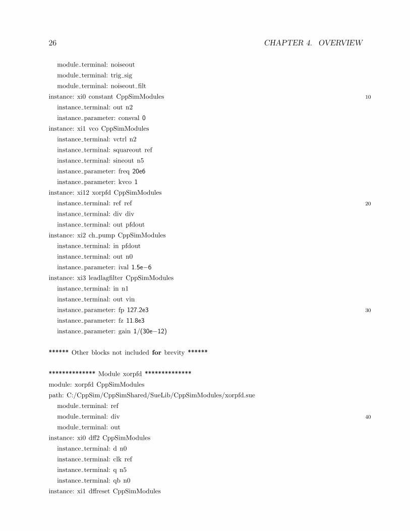
26 CHAPTER 4. OVERVIEW
module terminal: noiseout
module terminal: trig sig
module terminal: noiseout filt
instance: xi0 constant CppSimModules 10
instance terminal: out n2
instance parameter: consval 0
instance: xi1 vco CppSimModules
instance terminal: vctrl n2
instance terminal: squareout ref
instance terminal: sineout n5
instance parameter: freq 20e6
instance parameter: kvco 1
instance: xi12 xorpfd CppSimModules
instance terminal: ref ref 20
instance terminal: div div
instance terminal: out pfdout
instance: xi2 ch pump CppSimModules
instance terminal: in pfdout
instance terminal: out n0
instance parameter: ival 1.5e−6
instance: xi3 leadlagfilter CppSimModules
instance terminal: in n1
instance terminal: out vin
instance parameter: fp 127.2e3 30
instance parameter: fz 11.8e3
instance parameter: gain 1/(30e−12)
****** Other blocks not included for brevity ******
************** Module xorpfd **************
module: xorpfd CppSimModules
path: C:/CppSim/CppSimShared/SueLib/CppSimModules/xorpfd.sue
module terminal: ref
module terminal: div 40
module terminal: out
instance: xi0 dff2 CppSimModules
instance terminal: d n0
instance terminal: clk ref
instance terminal: q n5
instance terminal: qb n0
instance: xi1 dffreset CppSimModules
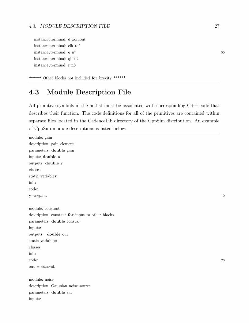
4.3. MODULE DESCRIPTION FILE 27
instance terminal: d xor out
instance terminal: clk ref
instance terminal: q n7 50
instance terminal: qb n2
instance terminal: r n8
****** Other blocks not included for brevity ******
4.3 Module Description File
All primitive symbols in the netlist must be associated with corresponding C++ code that
describes their function. The code definitions for all of the primitives are contained within
separate files located in the CadenceLib directory of the CppSim distribution. An example
of CppSim module descriptions is listed below:
module: gain
description: gain element
parameters: double gain
inputs: double a
outputs: double y
classes:
static variables:
init:
code:
y=a∗gain; 10
module: constant
description: constant for input to other blocks
parameters: double consval
inputs:
outputs: double out
static variables:
classes:
init:
code: 20
out = consval;
module: noise
description: Gaussian noise source
parameters: double var
inputs:

28 CHAPTER 4. OVERVIEW
outputs: double out
static variables:
classes: Rand randg("gauss")
init: 30
code:
out = sqrt(var/Ts)∗randg.inp();
module: step in
description: step input
parameters: double vend double vstart double tstep
inputs:
outputs: double step
classes:
static variables: double i 40
init: i=0.0;
code:
step = i∗Ts > tstep ? vend : vstart;
i++;
module: vco
description: voltage controlled oscillator
parameters: double freq double kvco
inputs: double vctrl
outputs: double squareout double sineout 50
static variables:
classes: Vco vco("fc + Kv*x","fc,Kv,Ts",freq,kvco,Ts);
init:
code:
vco.inp(vctrl);
squareout = vco.out;
sineout = sin(vco.phase);
module: leadlagfilter
description: lead/lag filter 60
parameters: double fz, double fp, double gain
inputs: double in
outputs: double out
static variables:
classes: Filter filt("1+1/(2*pi*fz)s","C3*s + C3/(2*pi*fp)*s^2","C3,fz,fp,Ts",1/gain,fz,fp,Ts);
init:
code:
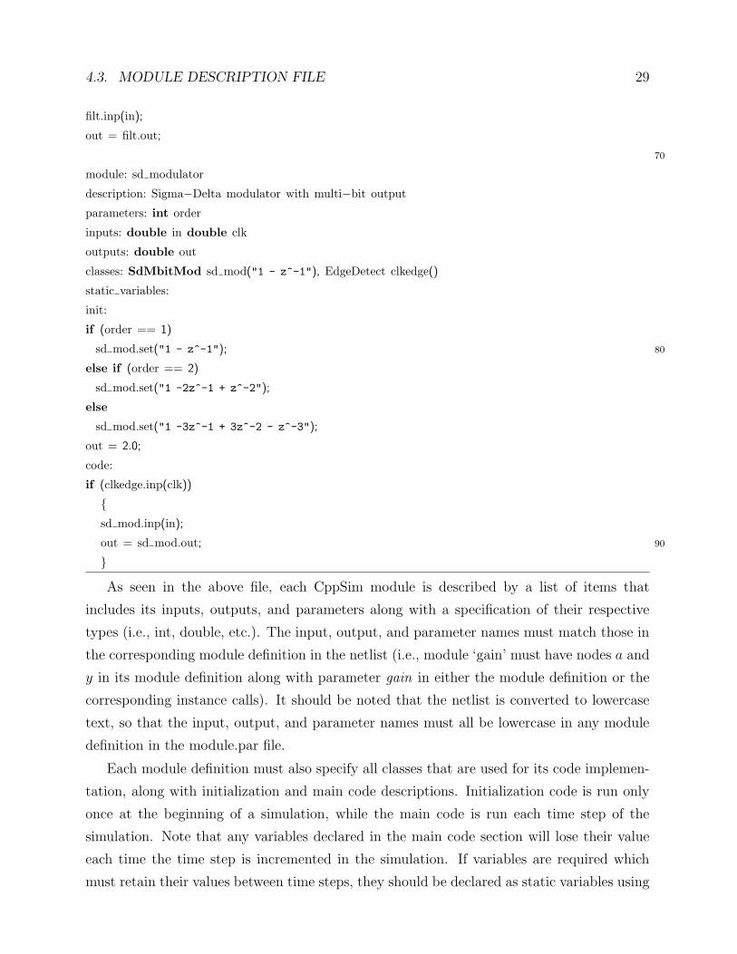
4.3. MODULE DESCRIPTION FILE 29
filt.inp(in);
out = filt.out;
70
module: sd modulator
description: Sigma−Delta modulator with multi−bit output
parameters: int order
inputs: double in double clk
outputs: double out
classes: SdMbitMod sd mod("1 - z^-1"), EdgeDetect clkedge()
static variables:
init:
if (order == 1)
sd mod.set("1 - z^-1"); 80
else if (order == 2)
sd mod.set("1 -2z^-1 + z^-2");
else
sd mod.set("1 -3z^-1 + 3z^-2 - z^-3");
out = 2.0;
code:
if (clkedge.inp(clk))
{sd mod.inp(in);
out = sd mod.out; 90
}As seen in the above file, each CppSim module is described by a list of items that
includes its inputs, outputs, and parameters along with a specification of their respective
types (i.e., int, double, etc.). The input, output, and parameter names must match those in
the corresponding module definition in the netlist (i.e., module ‘gain’ must have nodes a and
y in its module definition along with parameter gain in either the module definition or the
corresponding instance calls). It should be noted that the netlist is converted to lowercase
text, so that the input, output, and parameter names must all be lowercase in any module
definition in the module.par file.
Each module definition must also specify all classes that are used for its code implemen-
tation, along with initialization and main code descriptions. Initialization code is run only
once at the beginning of a simulation, while the main code is run each time step of the
simulation. Note that any variables declared in the main code section will lose their value
each time the time step is incremented in the simulation. If variables are required which
must retain their values between time steps, they should be declared as static variables using

30 CHAPTER 4. OVERVIEW
the ‘static variables:’ command.
Please see Chapter 6 for more information on writing module description files, which
includes issues related to syntax and information on the various commands that are available.
4.4 Simulation Description File (test.par)
The overall systems parameters, such as number of time steps and the simulation step size
are specified in a simulation description file that we will refer to as ‘test.par’. An example
test.par file is given below:
num sim steps: 2e6
Ts: 1/10e9
∗∗ save most signals every time step
output: signals
probe: out ref vin pfdout sd in xi12.xor out
∗∗ save sd modulator output only on rising edges of divider output
output: sd out trigger=div
probe: div val
10
global param: in gl=92.31793713 delta gl=4 step time gl=.7e6∗Tsglobal nodes: vdd=1.0 gnd=−1.0
∗ top param: x=in gl+2.0
∗ alter: delta gl=1:0.25:4
∗ inp timing: 1e−9 .5e−9 1/2e9 0 1
∗ inp dig: node1 [1 0 1 (0 3) (1 4) 0]
∗ inp dig: node2 [1 0 0 (1 3) (0 5) 1]
Please see Chapter 5 for more information on writing simulation description files, which
includes issues related to syntax and information on the various commands that are available.
4.5 CppSim Commands
The recommended method of running CppSim is from its GUI interface in Sue2 (or Cadence).
Alternatively, it can be run from Matlab or a command prompt in a manner such that
minimal effort is required of the user to run simulations. See the Setup section (Chapter 3)
for details. Note that, upon completion of the simulation, you can view the results using
CppSimView, GTKWave, or Matlab (using the Hspice Toolbox included with this package).
4.6. VIEWING RESULTS 31
4.6 Viewing Results
The output of the CppSim simulation run is in Hspice-compatible binary format by default,
and is stored for this example in the files ‘signals.tr0’ and ‘sd out.tr0’ as directed by the ‘out-
put:’ commands in the above ‘test.par’ file. To view signals, one can either use CppSimView
or the Hspice Toolbox for Matlab that is included with the CppSim package. Documentation
for the Hspice Toolbox is included as an appendix at the end of this document. Note that the
output can also be specified as an LXT file which GTKWave can read. See the description
for the ‘output:’ command in the following section for more information on this option.
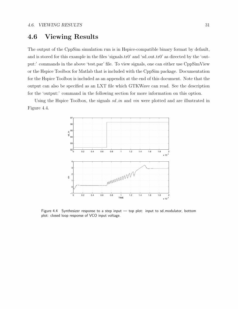
Using the Hspice Toolbox, the signals sd in and vin were plotted and are illustrated in
Figure 4.4.
0 0.2 0.4 0.6 0.8 1 1.2 1.4 1.6 1.8 2
x 10−4
92
93
94
95
96
97
sd_i
n
0 0.2 0.4 0.6 0.8 1 1.2 1.4 1.6 1.8 2
x 10−4
−1
0
1
2
3
4
vin
TIME
Figure 4.4 Synthesizer response to a step input — top plot: input to sd modulator, bottomplot: closed loop response of VCO input voltage.

32 CHAPTER 4. OVERVIEW

Chapter 5
Specifying Simulation Parameters
(test.par)
This chapter discusses the various commands available for use in the simulation description
file, which we refer to as the ‘test.par’ file. We begin by covering general parsing issues,
including the notation for commenting out lines, and will then discuss the various commands
in detail.
5.1 Parsing Rules
The CppSim environment is designed to be very forgiving with respect to parsing rules so
that one does not need to remember adding commas or semicolons at the right place. In
general, spaces are used to separate commands from their arguments, as well as arguments
from each other, and commas and semicolons are ignored. As an example, the statement
global param: a gl=3.3 b gl=-5 c gl=.7e6*Ts
can also be written as
global param: a gl = 3.3 b gl = -5 c gl = .7e6*Ts
or as
global param: a gl=3.3, b gl=-5, c gl=.7e6*Ts;
or as
global param:
a gl=3.3
b gl=-5
c gl=.7e6*Ts
33

34 CHAPTER 5. SPECIFYING SIMULATION PARAMETERS (TEST.PAR)
As a rule of thumb, one should never separate an expression into multiple lines. As an
example, you should NOT write
global param: a gl=
3.3
‘//’ characters can be used to comment out lines provided that they are the first characters
encountered on a line. As an example
// global param: a gl=3.3 b gl=-5 c gl=.7e6*Ts
///// global param: a gl=3.3 b gl=-5 c gl=.7e6*Ts
are valid ways of commenting out a line.
Descriptions of the individual commands used in a ‘test.par’ file are presented below:
5.2 num sim steps:
The number of simulation steps is specified with this statement. An example of the syntax
of this command is:
num sim steps: 2e6
5.3 Ts:
The value of the simulation period, Ts, is specified with this statement. Note that Ts
becomes a global variable in the C++ simulation code, and is often used in module parameter
statements as well as module code. An example of the syntax of this command is:
Ts: 1/10e9
5.4 output:
The name of the Hspice-compatible binary output file for signals specified in the following
‘probe:’ or ‘probe64:’ statement. Nominally, the specified signals are stored every time step
of the simulator. Optional parameters allow one to store the signal values only on the rising
or falling edges of a trigger signal, when an enable signal is above zero, or when the time
sample or time value is greater than or equal to a given value. You can also save to a format
that supports CppSimView and the Hspice Toolbox for Matlab (which are convenient for
analog signal viewing and processing), or to a format that supports GTKWave (which is
convenient for viewing digital signals). A summary of the available options is

5.4. OUTPUT: 35
• Save for GTKWave (i.e., lxt file format)
filetype=gtkwave
• View double interp signals as boolean values (i.e., 0 or 1)
view double interp=bool
• Save only on positive edges of signal ’trig sig’
trigger=trig sig
• Save only on negative edges of signal ’trig sig’
trigger=-trig sig
• Save only when ’enable sig’ is greater than 0
enable=enable sig
• Save when ’enable sig’ is less than or equal to 0
enable=-enable sig
• Save when simulation step is within a simulation time step range
start sample=sample num to begin end sample=sample num to end
• Save when simulation step is within a simulation time range
start time=sample time to begin end time=sample time to end
• Save only when bool or double interp signals transition
dig transitions=max time between samples
Example: save signals every time step in the binary file ‘signals.tr0’ which can be viewed
with CppSimView or the Hspice Toolbox for Matlab
output: signals
probe: a b y xi12.net12
Example: save signals every time step in the binary file ‘signals 0.lxt’ which can be viewed
with GTKWave

36 CHAPTER 5. SPECIFYING SIMULATION PARAMETERS (TEST.PAR)
output: signals filetype=gtkwave
probe: a b y xi12.net12
Example: save signals only when the signal ‘xi1.clk’ has a rising edge in the CppSimView
file ‘signals2.tr0’
output: signals2 trigger=xi1.clk
probe: a2 b2 xi3.xi1.sd out
Example: save signals only when the signal ‘clk’ has a falling edge in the GTKWave file
‘signals3.tr0’, and view double interp signals as bool values (i.e., either 0 or 1 rather than -1
to 1)
output: signals3 filetype=gtkwave view double interp=bool trigger=-xi1.clk
probe: a2 b2 xi3.xi1.sd out
Example: save signals only when the signal ‘clk’ is greater than zero in the binary file
‘signals3.tr0’
output: signals3 enable=xi1.clk
probe: a2 b2 xi3.xi1.sd out
Example: save signals only when the signal ‘clk’ is less than or equal to zero in the binary
file ‘signals3.tr0’
output: signals3 enable=-xi1.clk
probe: a2 b2 xi3.xi1.sd out
Example: save signals only when bool or doube interp signals within the probe list transition,
with a maximum time between samples of 1 microsecond
output: signals2 dig transitions=1/1e6
probe: a2 b2 xi3.xi1.sd out
Example: save signals only when the simulation time step is greater than or equal to 1000
output: signals3 start sample=1000
probe: a2 b2 xi3.xi1.sd out
Example: save signals only when the simulation time value is greater than or equal to 1e-6
output: signals3 start time=1e-6
probe: a2 b2 xi3.xi1.sd out
Example: save signals only when the simulation time step is less than or equal to 3000
output: signals3 end sample=3000
probe: a2 b2 xi3.xi1.sd out

5.5. PROBE: 37
Example: save signals only when the simulation time value is less than or equal to 3e-6
output: signals3 end time=3e-6
probe: a2 b2 xi3.xi1.sd out
Example: save to multiple files
output: signals
probe: a b y xi12.net12
output: signals2 trigger=xi1.clk enable=sig1
probe: a2 b2 xi3.xi1.sd out
output: signals3 trigger=-xi1.clk start time=1e-6 end time=3e-6
probe: a2 b2 xi3.xi1.sd out
output: signals3 filetype=gtkwave view double interp=bool trigger=xi1.clk
probe: a2 b2 xi3.* xi3.xi1.*
Note that in all cases, the trigger signal must be a square wave that alternates between
either -1 and 1, 0 and 1, or 0 and -1 (see the description of the EdgeDetect class).
5.5 probe:
The signals specified with this statement are saved in a binary file according to the infor-
mation specified by the last ‘output:’ command encountered before this statement. Signals
contained in the top level of the schematic are specified by their name, and signals at lower
levels of hierarchy are specified by their name and by the chain of instances that lead to the
cell view that the signal is contained in. An example of the syntax of this command is:
probe: vin pfdout sd in div val xi12.xor out xi12.xi7.y
where xi12.xor out corresponds to signal xor out contained within instance xi12 in the top
level of hierarchy, and xi12.xi7.y corresponds to signal y contained within instance xi7 that
is within instance xi12. Note that the number of levels of hierarchy within the system can
be as large as the user desires.
Wild card characters can also be used in specifying probe node names. For instance, to
record all signals in the top view of the system as well as all signals within instance xi1, you
would specify
probe: * xi1.*
Note that if you specify just an instance name (such as xi2), then all of the input and output
signals of that instance will be probed

38 CHAPTER 5. SPECIFYING SIMULATION PARAMETERS (TEST.PAR)
probe: * xi1.* xi2
For Verilog modules only (which are automatically converted to C++ by Verilator), you can
specify multiple levels of probing. For instance, to look at all of the signals within the first
2 levels of hierarchy within Verilog instance xi3, you would specify
probe: * xi1.* xi2 xi3.*.*
5.6 probe64:
The same as ‘probe:’, except that values are stored as 64-bit values rather than 32-bit values.
Files created with ‘probe64:’ are roughly twice as large as those created with ‘probe:’, but
provide double-precision rather than single-precision accuracy for signals.
An example of the syntax of this command is:
probe64: vin pfdout sd in div val xi12.xor out xi12.xi7.y
Note that this option is not valid when saving to GTKWave file format (i.e., lxt files).
5.7 global nodes:
A global node is assumed to have a constant signal value across all levels of hierarchy. The
signal value of such nodes are specified with this statement. For example, nodes that are
named vdd and gnd can be specified to have signal levels 1.0 and -1.0, respectively, using
the statement:
global nodes: vdd=1.0 gnd=-1.0
In practice, it is inappropriate for global nodes to correspond to the output node of any
instance — they should always correspond to input nodes. No checking is done to insure
this is the case.
5.8 global param:
Global parameters are defined at all levels of hierarchy in the system. These parameters can
be used within parameter expressions, and can also be used within module code (although
that is not generally recommended). It is suggested that the user label these parameters in
a manner that reflects the fact that they are global, such as by adding the suffix ‘ gl’ to their
names. Note that the variable Ts is automatically supplied as a global parameter, and its
value is set according to the ‘Ts:’ statement described above. An example of the syntax of
this command is:

5.9. TOP PARAM: 39
global param: a gl=3.3 b gl=-5 c gl=.7e6*Ts
5.9 top param:
Top level parameters are defined only in the top level of the system hierarchy. Therefore,
this command would be used instead of the ‘global param:’ command if one wanted to
constrain the scope of a parameter to the top level as opposed to having it pervade all levels
of hierarchy. These parameters cannot be altered using the ‘alter:’ command described
below, but can be defined in terms of global parameters which can be altered. An example
of the syntax of this command is:
top param: yval=1/4e9 xval=a gl+2.0
5.10 alter:
You can alter global parameters several ways using the ‘alter:’ statement, which will now be
explained through a series of examples. In all of the examples, the ‘alter:’ statement(s) are
assumed to be placed after the ‘global param:’ statement that defines the global parameters
being altered.
Example: do simulations over all combinations of a gl = 15,18 and b gl = 1e3,2e3
alter: a gl = 15 18
alter: b gl = 1e3 2e3
Example: do simulations where a gl and b gl are altered together,
i.e., a gl,b gl = 15,1e3 and a gl,b gl = 18,2e3
alter: a gl = 15 18 b gl = 1e3 2e3
Example: do combinations where a gl and b gl are altered together in combination with
values of c gl = 1,2,3,4,5
alter: a gl = 15 18 b gl = 1e3 2e3
alter: c gl = 1 2 3 4 5
Example: an easier way to do the above is to use Matlab notation:
alter: a gl = 15 18 b gl = 1e3 2e3
alter: c gl = 1:5
Example: suppose you want to increment c gl by 0.1 instead of 1

40 CHAPTER 5. SPECIFYING SIMULATION PARAMETERS (TEST.PAR)
alter: c gl = 1:0.1:5
Example: combine Matlab notation with individual specifications
alter: c gl = 1e3 5e3:1e3:10e3 20e3 50e3 100e3:100e3:1e6 2e6
The resulting output of performing such ‘alter:’ operations is to produce a separate
output file for each global parameter combination. As an example, if
output: signals
is specified in the test.par file, then a a series of files
signals.tr0 signals.tr1 signals.tr2 . . .
will be produced. If you have multiple ‘output:’ statements, then a series of files will be
produced for each of those output files.
To see how the global variable combinations match up to their corresponding transient
runs in this case, you can load test globals.tr0 in Matlab. Note that the prefix ’test’ was
determined by the name of the simulation description file, ’test.par’. If you instead, as an
example, named this file ’test2.par’, you would load test2 globals.tr0. Each altered global
variable will be a signal in that file whose value for each simulation run is specified.
5.11 inp timing:
Input signals into the simulated system should generally be created within the graphical
environment of the schematic capture program. However, there are cases where it is easier
to specify signals directly in the test.par file. Specifically, digital signals are easier to specify
in an ASCII editor as a vector sequence than by going through the graphical environment.
In the future, other types of signals may also be supported.
The ‘inp timing:’ command is used to specify the timing parameters associated with
input signals that follow it. The parameters of this command are as follows:
inp timing: delay rise/fall time period vlow vhigh
In the above statement, ‘delay’ corresponds to the initial delay of the waveform, ‘rise/fall time’
corresponds to its rise and fall times, ‘period’ is its period in seconds, and ‘vlow’ and
‘vhigh’ are its minimum and maximum signal values. Currently, digital inputs ignore the
rise/fall time parameter, but all of the parameters must still be specified. An example of
the syntax of this command is:
inp timing: 1e-9 .5e-9 1/2e9 0 1
Note that the inp timing command can NOT span over multiple lines.
5.12. INP DIG: 41
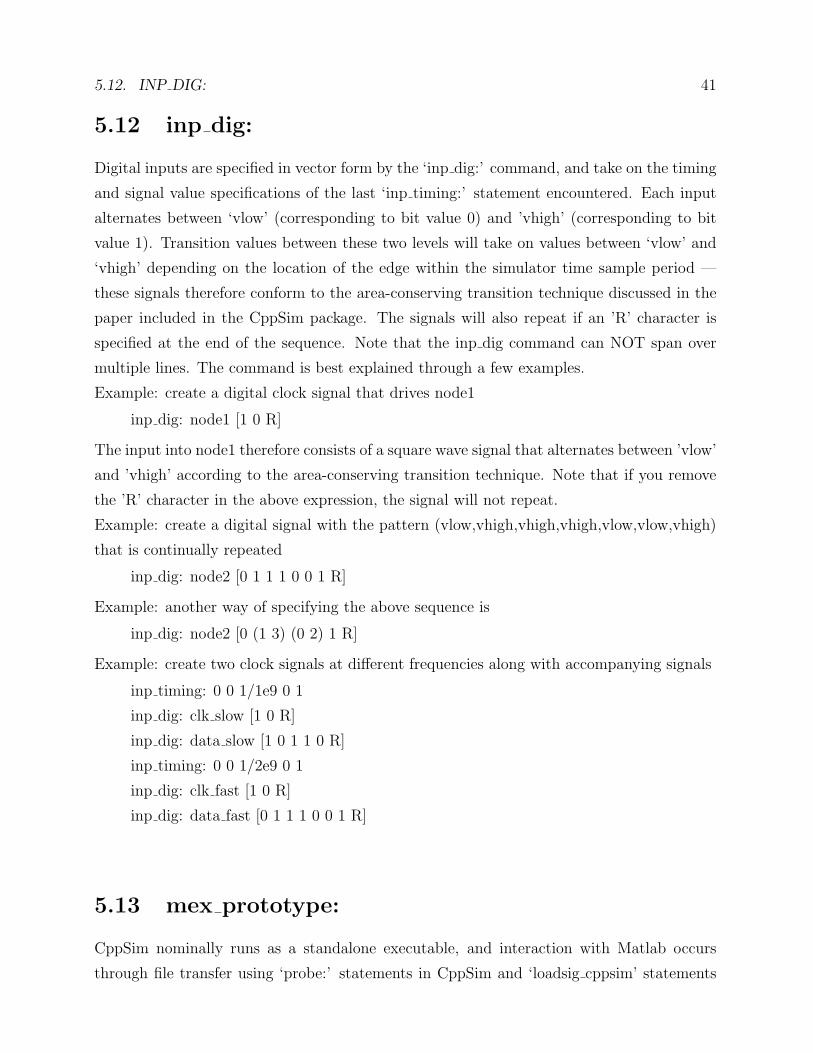
5.12 inp dig:
Digital inputs are specified in vector form by the ‘inp dig:’ command, and take on the timing
and signal value specifications of the last ‘inp timing:’ statement encountered. Each input
alternates between ‘vlow’ (corresponding to bit value 0) and ’vhigh’ (corresponding to bit
value 1). Transition values between these two levels will take on values between ‘vlow’ and
‘vhigh’ depending on the location of the edge within the simulator time sample period —
these signals therefore conform to the area-conserving transition technique discussed in the
paper included in the CppSim package. The signals will also repeat if an ’R’ character is
specified at the end of the sequence. Note that the inp dig command can NOT span over
multiple lines. The command is best explained through a few examples.
Example: create a digital clock signal that drives node1
inp dig: node1 [1 0 R]
The input into node1 therefore consists of a square wave signal that alternates between ’vlow’
and ’vhigh’ according to the area-conserving transition technique. Note that if you remove
the ’R’ character in the above expression, the signal will not repeat.
Example: create a digital signal with the pattern (vlow,vhigh,vhigh,vhigh,vlow,vlow,vhigh)
that is continually repeated
inp dig: node2 [0 1 1 1 0 0 1 R]
Example: another way of specifying the above sequence is
inp dig: node2 [0 (1 3) (0 2) 1 R]
Example: create two clock signals at different frequencies along with accompanying signals
inp timing: 0 0 1/1e9 0 1
inp dig: clk slow [1 0 R]
inp dig: data slow [1 0 1 1 0 R]
inp timing: 0 0 1/2e9 0 1
inp dig: clk fast [1 0 R]
inp dig: data fast [0 1 1 1 0 0 1 R]
5.13 mex prototype:
CppSim nominally runs as a standalone executable, and interaction with Matlab occurs
through file transfer using ‘probe:’ statements in CppSim and ‘loadsig cppsim’ statements
42 CHAPTER 5. SPECIFYING SIMULATION PARAMETERS (TEST.PAR)
in Matlab. However, there are times when it is more convenient to work directly with a
CppSim object in Matlab. The ‘mex prototype:’ command allows automatic generation of
a Matlab mex file corresponding to a given CppSim system which can then be compiled and
run directly in Matlab.
An example of the syntax of this command is:
mex prototype: [vin,xi12.xor out] = sd synth fast(in,in2,param1,num sim steps,Ts);
In the above example, signals vin and xi12.xor_out correspond to signals which have been
placed within ‘probe:’ statements elsewhere in the simulation file. These signals will be
output by the above Matlab mex call upon its completion — all conditions imposed by the
associated ‘probe:’ statements for each signal will be observed (such as triggering or enabling
by other signals, start and stop times, etc.) so that the vector lengths of each of these signals
may differ from each other.
The name of the mex function, which in the above case is ‘sd synth fast’, must be the
same as the associated CppSim top level cell.
The input signals in and in2 can have different lengths in the above case since num_sim_steps
is specified, but must have the same length if num_sim_steps is not present in the prototype
definition. Both global and top cell parameters, such as param1 in the above example, can
be specified. The specification of num_sim_steps and Ts are optional. If num_sim_steps is
not specified, then the number of simulation steps per mex call will be set by the length of
the input signals. If num_sim_steps is not specified and no input signals are present, then
the number of simulation steps per mex call will be the same as specified in the simulation
file (i.e., test.par). If Ts is not specified, then the simulation step size will also be as specifed
in the simulation file.
Repeated calls to the CppSim mex function will cause the simulation to continue from
its last stopping point. To reset the simulation to its starting point, you must specify ‘end’
within the mex call. For the above example, you would run
sd synth fast(‘end’);
within Matlab. Resetting the simulation allows parameters (including num_sim_steps and
Ts) to be updated. In contrast, input signals can be changed for each mex call regardless of
whether the simulation has been reset.
Setting Up the Mex Compiler in Matlab (under Windows)
To set up the mex compiler in Matlab, run the command
mex -setup

5.13. MEX PROTOTYPE: 43
In Windows, you need to specify a C++ compiler rather than the C compiler that comes
with Matlab. Thus far, only the Microsoft C++ compiler has been verified to work — a free
version of this compiler is available at
http://msdn.microsoft.com/vstudio/express/visualc/
After downloading this package, you’ll need to add a few missing library files to the directory
c:/Program Files/Microsoft Visual Studio 8/VC/lib
which, for convenience, have been placed within the CppSim package (Windows version) in
the directory
c:/CppSim/CommonCode/msft_SDK
Setting Up the Mex Compiler in Matlab (Cadence Version in Linux)
To set up the mex compiler in Matlab, run the command
mex -setup
Choose the Template Options file for buiding gcc MEX-files (i.e., gccopts.sh).
Generating and Compiling the Mex Function in Matlab
To generate the mex code, you simply need to include the ‘mex prototype:’ statement
within the simulation file (i.e., test.par) and then run cppsim. To do this in Matlab, begin by
changing the working directory to that of the desired SimRun cellview and then run cppsim
within Matlab. To access the cppsim script in Matlab, recall that you need to first add the
HspiceToolbox path to Matlab using the Matlab command:
addpath c:/cppsim/HspiceToolbox
As an example, in Matlab you might type
cd c:/CppSim/SimRuns/Synthesizer_Examples/sd_synth_fast
and then run cppsim within Matlab in that directory.
To compile the mex function after completion of the CppSim run, you would then run
the Matlab command
compile_sd_synth_fast
where you should replace the above with compile_cellname for a cellname other than
sd_synth_fast. Upon completion of the above, you can then run the mex function in
Matlab as specified by the prototype format.
Additional Examples
Here are additional examples of the syntax of the ‘mex prototype:’ command:

44 CHAPTER 5. SPECIFYING SIMULATION PARAMETERS (TEST.PAR)
mex prototype: [vin] = sd synth fast();
In the above case, num_sim_steps and Ts are set according to the simulation file (i.e.,
test.par).
mex prototype: [vin] = sd synth fast(in,in2);
In the above case, Ts is set according to the simulation file (i.e., test.par), and num_sim_steps
is set equal to the lengths of input signals in and in2 (which must have matching lengths).
mex prototype: [vin] = sd synth fast(in,in2,num sim steps);
In the above case, Ts is set according to the simulation file (i.e., test.par), num_sim_steps is
set according to the above input value, and in and in2 can be input signals of any length. As
an example, consider the case where num_sim_steps was set to 1000, the length of in to 10,
and the length of in2 to 20. In this case, each mex call with such settings will progressively
simulate the system 1000 steps at a time, where the first 10 steps will progress through the
first 10 input values of in and in2, the next 10 steps will retain the last value of in while
it progresses through the next 10 values of in2, and the remaining steps will retain the last
values of in and in2. Therefore, by declaring num_sim_steps as one of the input arguments
to the mex function, one can avoid long input vector lengths for the case where input signals
are constant.
Vector Input and Output Signals
Sometimes it is desirable to have input or output signals of type Vector or IntVector
for the CppSim mex function in Matlab. In such case, it is important to realize that input
and outputs are treated quite differently when they are CppSim vector signals. In the
case of input vector signals, they must have constant length for the entire duration of a
given simulation run (i.e., until the user calls the ‘end’ command discussed above), and are
assumed to be constant for the duration of each mex call. The length of such input vectors
do not influence the value of num_sim_steps as inputs with non-vector types can. In the
case of output vector signals, they will also be restricted to have constant length for the
entire duration of a simulation run (i..e, until the user calls the ‘end’ command), but are not
assumed to be constant for the duration of each mex call. In Matlab, these vector outputs
will be converted to matrices whose rows correspond to the vector array values at given time
instances, and whose columns correspond to different time instances.
As an example, suppose that signal in is a Vector signal of length 8, while signal in2
is a double signal of length 100. Suppose also that out1 corresponds to a Vector signal of
length 10, whereas out2 corresponds to a double signal. Assume that we specify the mex
function prototype as:
5.14. SIMULINK PROTOTYPE: 45
mex prototype: [out1,out2] = sd synth fast(in,in2);
When the above mex function is called in Matlab, the value of num_sim_steps is set to be
100 (corresponding to the length of the non-vector signal in2). The value of in is assumed
to be an 8-element vector that is constant for the duration of the 100 time steps of each
mex call, whereas the value of in2 will vary at each time step according to its Matlab array
values. Output signal out1 will consist of a matrix with 10 rows and 100 columns, while
output signal out2 will consist of a vector with 1 row and 100 columns.
5.14 simulink prototype:
Similar to the ‘mex prototype:’ command, the ‘simulink prototype:’ command allows more
direct operation of CppSim code within the Matlab environment. The ‘simulink prototype:’
command allows automatic generation of a Simulink S-Function file corresponding to a given
CppSim system which can then be compiled and run directly in Simulink.
An example of the syntax of this command is:
simulink prototype: [vin,sd in] = sd synth fast(in,in2[3],in3[par2],par1,par2,Ts);
In the above example, signals vin and sd_in correspond to signals which have been placed
within ‘probe:’ statements elsewhere in the simulation file. These signals will correspond
to outputs in the resulting Simulink block. Unlike the ‘mex prototype:’ command, the
conditions imposed by the associated ‘probe:’ statements for each signal (such as triggering
or enabling by other signals, start and stop times, etc.) will be ignored. Also, unlike the
‘mex prototype:’ command, the parameter ‘Ts’ (which corresponds to the time step of the
CppSim code) must always be included as one of the Simulink parameters.
The name of the Simulink function call, which in the above case is ‘sd synth fast’, must
be the same as the associated CppSim top level cell. The final S-Function name will have
a ’ s’ appended to it (i.e., ‘sd synth fast s’ in the above example) so that there is no clash
between Simulink and mex files created for the same cell.
The input signals in and in2[3] correspond to scalar and vector signals, respectively.
All input vectors must have their lengths explicitly specified (i.e., in2[3] is a vector of
length 3). The length can be specified as a parameter, as shown in the above example where
in3[par2] is a vector of length par2. Any vectors which correspond to output signals from
the block will have their lenths automatically set by the CppSim code, so that that the user
cannot specify their length in the ‘simulink prototype:’ statement.

46 CHAPTER 5. SPECIFYING SIMULATION PARAMETERS (TEST.PAR)
To better understand the ‘simulink prototype:’ statement, please refer to the CppSim
Primer document. Also, please note that you must have a C++ compiler installed on your
system, as described in the ‘mex prototype:’ section of this document.
5.15 add top verilog libary file statements:
This command is used to place verilog library file statements in the top portion of the
test_lib.v file that is generated with the net2code -vpp command. You can use this
command to add standard cell library code when running VppSim simulations. Note that
this command is ignored when running CppSim simulations (i.e., net2code -cpp).
An example of the syntax of this command is:
add top verilog library file statements:
‘timescale 1ns/1ps
module example verilog module (a,b,y);
input a,b;
output y;
(· · · verilog module code · · ·)endmodule
module example verilog module2 (x,y);
(· · · verilog module code · · ·)endmodule
5.16 add bottom verilog libary file statements:
This command is essentially the same as the add_top_verilog_library_file_statements:
command except that the included statements are placed at the bottom of the test_lib.v
file rather than the top. Placement of the included statements at the bottom of the
test_lib.v file prevents included definition statements such as timescale from impact-
ing the auto-generated code by the net2code -vpp command.
5.17 add verilog test file statements:
This command is used to place verilog test file statements within the test.v file that is
generated with the net2code -vpp command. You can use this command to add ‘define,

5.18. ADD VERILOG TEST MODULE STATEMENTS: 47
‘include, and any other appropriate verilog statements within your VppSim testbench but
outside of the top testbench module. In contrast, you should use the add_verilog_test_module_statement
command to include statements within the verilog testbench module. Note that this com-
mand is ignored when running CppSim simulations (i.e., net2code -cpp).
An example of the syntax of this command is:
add verilog test file statements:
‘define CONV RATE 2’b10
‘include “/home/user/constants.v”
5.18 add verilog test module statements:
This command is used to place verilog test file statements within the top testbench module
in test.v file that is generated with the net2code -vpp command. You can use this com-
mand to add registers, wires, PLI calls, and any other appropriate verilog statements to the
VppSim testbench module. In contrast, you should use the
add_verilog_test_file_statements: command to include statements outside of the ver-
ilog testbench module but inside the test.v file. Note that this command is ignored when
running CppSim simulations (i.e., net2code -cpp).
An example of the syntax of this command is:
add verilog test module statements:
reg power on;
initial
begin
power on = 0;
#10
power on = 1;
#10
power on = 0;
#100
$example pli call(“example parameter”);
end

48 CHAPTER 5. SPECIFYING SIMULATION PARAMETERS (TEST.PAR)
5.19 ignore nodes output check:
This command is used to allow CppSim to run despite having internal nodes that are not
driven by the outputs of other blocks. In general, it is suggested that this option only be
used in special circumstances since it can easily lead to systems whose blocks are incorrectly
wired.
An example of the syntax of this command is:
ignore nodes output check: yes
5.20 allow verilog output clashing:
This command is used to allow CppSim to run despite having output nodes of Verilog
modules connected together. In general, it is suggested that this option only be used in
special circumstances since it can easily lead to systems whose blocks are incorrectly wired.
An example of the syntax of this command is:
allow verilog output clashing: yes
5.21 allow non bool signals in bus:
This command is used to prevent CppSim from automatically converting signals which form a
bus (i.e., sig[5:0]) at the schematic level to bool signal values. Setting this option is primarily
useful to keep the timing information of double interp signals which are grouped together in
a bus at the schematic level.
An example of the syntax of this command is:
allow non bool signals in bus: yes
5.22 electrical integration damping factor:
This command alters the manner in which numerical integration is performed with the
two extremes being backward Euler integration (the default) and trapezoidal integration.
Backward Euler, which corresponds to a damping factor of 1.0, is chosen as the default since
it is well behaved for signals that contain fast transitions. For cases where signals do not
exhibit fast transitions, and especially for highly resonant networks, trapezoidal integration,
which corresponds to a damping factor of 0.0, is the better choice.
Some examples of using this command are:

5.23. TEMPERATURE CELSIUS FOR NOISE CALC: 49
electrical integration damping factor: 0.0
electrical integration damping factor: 1.0
electrical integration damping factor: 0.5
Note that schematic-based modules that are instantianted within a given system can
individually choose their electrical integration damping factor by including it as a parameter
in their icon view. An example of this approach is given in the cell test electrical rc filters
within library Electrical Examples.
5.23 temperature celsius for noise calc:
This command selects the temperature at which noise calculations are carried out for elec-
trical elements which include noise (i.e., resistors and electrical switches). The default value
is 25 degrees Celsius.
Some examples of using this command are:
temperature celsius for noise calc: -40.0
temperature celsius for noise calc: 125.0
50 CHAPTER 5. SPECIFYING SIMULATION PARAMETERS (TEST.PAR)

Chapter 6
Writing Code for Primitives
This chapter discusses the various commands available for use in the module code description
files, which are located in the CadenceLib directory. We begin by covering general parsing
issues, including the notation for commenting out lines, and will then discuss the various
commands in detail.
6.1 Parsing Rules
As in the case of the ‘test.par’ file, the CppSim environment is designed to be very forgiving
with respect to parsing rules for module code definitions so that one does not need to
remember adding commas or semicolons at the right place. In general, spaces are used to
separate commands from their arguments, as well as arguments from each other, and commas
and semicolons are ignored. As an example, the statement
inputs: double a double b
can also be written as
inputs: double a, double b;
or as
inputs:
double a
double b
As a rule of thumb, one should never separate a specific description into multiple lines. As
an example, you should NOT write
51

52 CHAPTER 6. WRITING CODE FOR PRIMITIVES
inputs: double
a
‘//’ characters can be used to comment out lines provided that they are the first characters
encountered on a line.
Example: comment out specific lines in a module description:
module: xor2
description: two-input xor gate
// parameters: double w
inputs: double a, double b
outputs: double y
classes: Xor xor1()
// init:
y = -1.0;
code:
xor1.inp(a,b);
y = xor1.out;
Example: comment out entire module description:
// module: xor2
description: two-input xor gate
parameters: double w
inputs: double a, double b
outputs: double y
classes: Xor xor1()
init:
y = -1.0;
code:
xor1.inp(a,b);
y = xor1.out;
Descriptions of the individual commands used to describe module code are presented
below:
6.2 module:
The name of the module specified here must match the associated module it represents in
the netlist. An example of the syntax of this command is:

6.3. DESCRIPTION: 53
module: and2
6.3 description:
A text description of the module function. This is ignored by CppSim, but is useful for
sharing the code with others. An example of the syntax of this command is:
description:
implements a two input ‘and’ function whose signals conform
to the area conservation protocol for representing transitions
6.4 label as usrp module:
CppSim has been set up to work with the USRP board designed by Matt Ettus (http://www.ettus.com).
There are some extra files that must be compiled in when USRP modules are included within
a CppSim system, and the ’label as usrp module:’ command allows auto-sensing of the need
for such extra compile steps. An example of the syntax of this command is:
label as usrp module: yes
label as usrp module: no
6.5 parameters:
The type and name of all parameters associated with the module are specified with this
command. The parameter names must match those in the associated module in the netlist
— since CppSim converts the netlist text to lowercase, lowercase parameter names must be
specified here. An example of the syntax of this command is:
parameters: double gain double fc int order
One should note that expressions for parameter values given in the netlist will be con-
verted to lowercase, so that it is good practice to define lowercase variables in the test.par
file. A related issue is that the global variable ’Ts’ has an uppercase letter — if you desire
to use it in expressions for parameter values within the netlist, then you should define a
lowercase version in the test.par file using
global param: ts=Ts

54 CHAPTER 6. WRITING CODE FOR PRIMITIVES
6.6 inputs:
The type and name of all inputs associated with the module are specified with this command.
The input names must match those in the associated module in the netlist description of the
module. An example of the syntax of this command is:
inputs: double a double b int c
6.7 outputs:
The type and name of all outputs associated with the module are specified with this com-
mand. The output names must match those in the associated module in the netlist de-
scription of the module. be specified here. An example of the syntax of this command is:
outputs: double y double yb int yd
6.8 classes:
The declaration statement of all classes used in the module code must be placed here. Any
number of classes can be specified, and parameters specified in the ‘parameters:’ statement
can be passed to class declaration expressions. A few examples are in order.
Example: declare two classes for use in the module code
classes: Reg reg1() Xor xor1()
or
classes:
Reg reg1()
Xor xor1()
Example: declare a class using parameters ‘freq’ and ‘kvco’ that have been specified with
the ‘parameters:’ command, and the global parameter ‘Ts’
classes: Vco vco(”fc + Kv*x”,”fc,Kv,Ts”,freq,kvco,Ts)
Note that a few words are in order with regards to syntax. First, all class objects must
have an associated set of parenthesis, as seen above with the class objects reg1() and xor1().
Second, class declarations cannot be broken up between lines, i.e., do NOT write:
classes: Vco vco(”fc + Kv*x”,”fc,Kv,Ts”,freq,
kvco,Ts)
6.9. STATIC VARIABLES: 55
6.9 static variables:
Since CppSim enters and exits the module code during each simulation time sample, variables
that are declared in the ‘code:’ section will go in and out of scope during each time sample,
and therefore will not retain their values from one simulation time step to the next. In the
case that you want to have a variable that retains its value from one simulation time step
to the next, you can declare it as a static variable using the ‘static variables:’ command. In
addition, static variables can be probed using the ‘probe:’ statement in the test.par file, and
therefore offer a means of probing signals embedded in the module code. An example of the
syntax of this command is:
static variables: double var1 int SigNum char Name[10]
Note that static variable names can freely use uppercase letters.
6.10 set output vector lengths:
The ‘set output vector lengths:’ command allows you to initialize the length of vectors that
are declared as output signals for the module. It is important to note that the length
of output vector signals cannot be changed except within the ‘set output vectors lengths:’
section — this is done so that vector lengths do not change during a given simulation alter
run, which would cause many headaches otherwise. (Note that vectors lengths can change
from alter run to alter run, just not within a given alter run). The output vector lengths
specified within the ‘set output vectors lengths:’ are valid before the ‘init:’ section is run,
which allows the length of input vector signals to be checked by code written in the ‘init:’
section.
To gain a better understanding of how to use this command, here is an example of setting
the output vector ’out vec’ to have length 8, and output vector ’out vec2’ to have length 12:
set output vector lengths:
out vec=8
out vec2=12
56 CHAPTER 6. WRITING CODE FOR PRIMITIVES
6.11 init:
The ‘init:’ command allows you to run initialization code that is executed only once at the
beginning of a simulation run (note that if you use the ‘alter:’ statement in the test.par file,
the initialization code will be run once for each global parameter combination). Therefore,
you can use this command to initialize variables and also to redefine class behavior based
on module parameters specified with the ‘parameters:’ command. For instance, the code
below redefines the noise shaping transfer function of a Σ-Δ modulator object based on the
module parameter ‘order’, and initializes the variable ‘out’ to the value of 2:
init:
if (order == 1)
sd mod.set(”1 - z-1”);
else if (order == 2)
sd mod.set(”1 -2z-1 + z-2”);
else
sd mod.set(”1 -3z-1 + 3z-2 - z-3”);
out = 2.0;
You can see the full module definition corresponding to the above ’init:’ command in Chapter
4, section 3.
An important issue in writing code in the ‘init:’ section is that it is not parsed by CppSim,
but rather is passed straight to the C++ simulation code. Therefore, the syntax of the code
must conform to the C++ language — if it does not, the C++ compiler will generate error
messages.
6.12 end:
The ‘end:’ command allows you to run terminating code that is executed only once at the
end of a simulation run (note that if you use the ‘alter:’ statement in the test.par file, the
terminating code will be run once for each global parameter combination). An example of
using the end: statement is found in the ascii store module within modules.par — there it
saves the contents of a list to a file at the end of a given simulation run.
An important issue in writing code in the ‘end:’ section is that it is not parsed by CppSim,
but rather is passed straight to the C++ simulation code. Therefore, the syntax of the code

6.13. CODE: 57
must conform to the C++ language — if it does not, the C++ compiler will generate error
messages.
6.13 code:
The ‘code:’ section contains the C++ code that implements the desired function of the
module. This code is run every time the simulator time step is incremented, and can include
variable declarations, functions, class objects, and all the standard C++ directives such as
for loops and if-else condition statements. One thing to be aware of is that if the user wants
to use their own user defined classes or functions, the class/function declarations must be
placed in the my classes and functions.h file and the class/function code must be placed in
the my classes and functions.cpp file, both of which must be located in the same directory as
cppsim classes.h and cppsim classes.cpp. The need for user defined classes/functions should
be minimal given the flexibility of the CppSim classes. Another issue is that variables
declared in the ‘code:’ section will lose their value from time step to time step, so that the
‘static variables:’ command should be used in some cases as discussed above. Finally, you
should be aware of the fact that the code specified in the ‘code:’ section is not parsed by
CppSim, but rather is passed straight to the C++ simulation code. Therefore, the syntax
of the code must conform to the C++ language — if it does not, the C++ compiler will
generate error messages.
Some examples are in order — each of the ones to follow are taken from the modules.par
file that is shown in Chapter 4, section 3.
Example: implement a ‘gain’ module by setting its output, ‘y’, equal to its input, ‘a’, times
a gain parameter ‘gain’:
code:
y=a*gain;
Example: implement a ‘noise’ module using a class object ‘randg’ (which implements a Gaus-
sian random sequence with variance one) whose output is scaled by the variance parameter
‘var’ and global variable ‘Ts’:
code:
out = sqrt(var/Ts)*randg.inp();
The reader is invited to look at more examples of ‘code:’ sections listed in Chapter 4, Section
3, as well as the various module descriptions contained in the CppSim package.

58 CHAPTER 6. WRITING CODE FOR PRIMITIVES
6.14 electrical element:
Provides an alternative to the ’code:’ command in describing the behavior of a module. In
particular, this command allows the module to correspond to an electrical element composed
of linear circuit components and/or switches. In turn, the values of the nodes for this
element are computed using nodal analysis. By allowing such electrical elements, CppSim
can simulate passive and active circuit networks, switched capacitor filters, and discrete-time
and continuous-time analog-to-digital converters.
Figure 6.1 shows the available electrical elements that may be used in CppSim. One
should note that they are all linear elements except for an ideal diode, electrical diode, and
switch, electrical switch, which are parameterized in terms of on and off resistance.
capacitor inductorresistor
1:n
electrical_transformer mutual_inductors
m
l1 l2
vcvsvccs cccs ccvs ccvs_single_out
electrical_diode electrical_switch dc_voltage dc_current
2
in2in
en
dc_current_with_noisedc_voltage_with_noise dc_voltage_with_noise_sq dc_current_with_noise_sq
en
Figure 6.1 Electrical elements available in CppSim.
The electrical primitives shown in Figure 6.1 are specified in the ‘electrical element:’
section of a CppSim module as follows:
• resistor t1 t2 resistance=resistance expr noise enable=noise enable expr
• capacitor t1 t2 capacitance=capacitance expr
• inductor t1 t2 inductance=inductor expr
6.14. ELECTRICAL ELEMENT: 59
• electrical transformer in ref in out ref out n=n expr
• mutual inductors t2 ref t2 t1 ref t1 inductance1=inductance1 expr inductance2=inductance2 expr
mutual inductance=mutual inductance expr
• vccs out ref out in ref in gain=gain expr
• cccs out ref out in ref in gain=gain expr
• vcvs out ref out in ref in gain=gain expr
• ccvs out ref out in ref in gain=gain expr
• ccvs single out out in ref in gain=gain expr
• electrical diode t1 t2 on resistance=on resistance expr off resistance=off resistance expr
• electrical switch t1 t2 sw on on resistance=on resistance expr off resistance=off resistance expr
noise enable=noise enable expr
• dc voltage v plus v minus dc voltage=dc voltage expr
• dc current plus minus dc current=dc current expr
• dc voltage with noise v plus v minus dc voltage=dc voltage expr noise enable=noise enable expr
spectral density=spectral density expr flicker corner frequency=flicker corner frequency expr
flicker slope=flicker slope expr
• dc voltage with noise sq v plus v minus dc voltage=dc voltage expr noise enable=noise enable expr
spectral density sq=spectral density sq expr flicker corner frequency=flicker corner frequency expr
flicker slope=flicker slope expr
• dc current with noise plus minus dc current=dc current expr noise enable=noise enable expr
spectral density=spectral density expr flicker corner frequency=flicker corner frequency expr
flicker slope=flicker slope expr
• dc current with noise sq plus minus dc current=dc current expr noise enable=noise enable expr
spectral density sq=spectral density sq expr flicker corner frequency=flicker corner frequency expr
flicker slope=flicker slope expr
60 CHAPTER 6. WRITING CODE FOR PRIMITIVES
Note that for the last four primitives, the parameter spectral density corresponds to
a single-sided spectral density with units of V/√Hz or A/
√Hz for dc voltage with noise
or dc current with noise, respectively. In contrast, the parameter spectral density sq corre-
sponds to a single-sided spectral density with units of V 2/Hz orA2/Hz for dc voltage with noise sq
or dc current with noise sq, respectively. Also, flicker corner frequency has units of Hertz,
and flicker slope has units of dB/decade and must have a value in the range of -5 to -15
(dB/decade).
As an example consider the following electrical element which corresponds to a resistor
with distributed parasitic capacitance:
module: resistor with cap
description:
parameters: double resistance, double noise enable, double par cap
inputs: double t1, double t2, double b
outputs:
classes:
static variables:
init:
code:
electrical element:
resistor t1 n0 resistance=resistance/2 noise enable=noise enable
resistor t2 n0 resistance=resistance/2 noise enable=noise enable
capacitor t1 b capacitance=par cap/4
capacitor n0 b capacitance=par cap/2
capacitor t2 b capacitance=par cap/4
Note that when CppSim runs, it will treat the above as an RC network inserted flat into
the corresponding schematic where the instance is placed.
6.15 functions:
The ‘functions:’ section allows you to specify functions local to the module being de-
fined. By doing so, the module becomes self-contained and easy to pass on to others (the
user otherwise needs to add such functions to my classes and functions.cpp/h in the Cpp-
Sim/CommonCode directory). To use the function within several different modules, you’ll

6.16. CUSTOM CLASSES DEFINITION: AND CUSTOM CLASSES CODE: 61
need to copy the function into the functions: section of each module (unless you put it into
my classes and functions.cpp/h).
As an example, let us assume that you wanted to use two functions within the module
called ‘add(a,b)’ and ‘mul(a,b)’. Such functions would be specified as:
functions:
double add(double a, double b)
{double out;
out = a + b;
return(out);
}double mul(double a, double b)
{double out;
out = a*b;
return(out);
}
6.16 custom classes definition: and custom classes code:
The ‘custom classes definition:’ and ‘custom classes code:’ sections allow you to specify
classes local to the module being defined. By doing so, the module becomes self-contained
and easy to pass on to others (the user otherwise needs to add such classes to the files
‘my classes and functions.cpp/h’ in the CppSim/CommonCode directory). To use the classes
within several different modules, you’ll need to copy the class definitions and code into the
custom classes definition: and custom classes code: sections of each module (unless you put
it into my classes and functions.cpp/h).
As an example, let us assume that you wanted to define a class called ‘And6 example’:
custom classes definition:
class And6 example
{public:
And6 example();
62 CHAPTER 6. WRITING CODE FOR PRIMITIVES
∼And6 example();
double inp(double in0, double in1, double in2, double in3, double in4, double in5);
double out;
private:
And and5,and2;
};
custom classes code:
And6 example::And6 example()
{out = -1.0;
}
And6 example::∼And6 example()
{}
double And6 example::inp(double in0, double in1, double in2, double in3, double in4, double in5)
{out = and2.inp(and5.inp(in0,in1,in2,in3,in4),in5);
return(out);
}
6.17 sim order:
As discussed in the Introduction chapter, CppSim executes each instance contained in a non-
primitive module (i.e. a module whose functionality is defined by the netlist rather than
by corresponding code in the modules.par file) one at a time until all have been executed,
updates the simulator time step, and then repeats the instance by instance execution. The
instance order in this execution sequence is nominally set by an algorithm internal to the
CppSim simulator. Generally, if the system does not contain feedback loops embedded within
other feedback loops, the algorithm does the right thing. However, if you do have a feedback

6.18. STOP CURRENT ALTER RUN 63
loop embedded within another feedback loop, you may want to bypass the algorithm and
directly specify the order of instance execution.
The ‘sim order:’ command allows you to specify the order of execution of the instances
in a non-primitive module. As an example, consider ordering the instances contained in the
‘xorpfd’ module specified in the netlist file in Chapter 4, Section 2. The module definition
within the modules.par file that would accomplish this task is given as:
module: xorpfd
sim order: xi1 xi2 xi3 xi5 xi4 xi7 xi8
Note that if you want to specify the order of instance execution in the top module in the
netlist (i.e., the highest cellview in the hierarchy), but your netlist does not include the
top module within a .subckt definition, then simply use the same description technique but
specify the module name as ‘top’, i.e.,
module: top
sim order: xi8 xi6 . . .
Note that the default behavior for the Sue2 setup is to include the top module within a
.subckt definition, in which case you refer to the top module by its schematic cell name
rather than by ‘top’.
CppSim will check that all instances are included in your list, and also alert you to any
instance names not being present in the associated netlist description of the module.
Note that there is an alternative method of specifying the order of execution of the
instances within a cell that does not involve changes to the modules.par file. Specifically,
CppSim reserves the parameter ‘sim order’ to specify the order of execution of instances
within a cell, so that the user may add this parameter to each instance and set the execution
order in their schematic editor. If this method is used, all instances in the cell must have
‘sim order’ as a parameter, and its value for a given instance should be set lower than the
values of other instances that should be executed after it. In other words, CppSim orders
the instances from lowest to highest ‘sim order’ value. One can use decimal values for the
‘sim order’ value, so that an instance with ‘sim order=1.5’ executes after an instance with
‘sim order=1’ and before an instance with ‘sim order=2’.
6.18 stop current alter run
In some cases it is desirable to stop a current alter run simulation after a given condition
is met. One can do this by simply asserting the ‘stop current alter run’ flag within any
module. An example is:

64 CHAPTER 6. WRITING CODE FOR PRIMITIVES
module: stop alter run on match
parameters:
inputs: int in1, int in2
outputs:
static variables:
classes:
init:
code:
if (in1 == in2)
{ 10
printf("Stop alter run asserted by 'stop_alter_run_on_match' module\n");
stop current alter run = 1;
}
6.19 timing sensitivity:
The ‘timing sensitivity:’ statement allows execution of the CppSim module code within the
‘code:’ section only when the conditions of this statement are met. As an example, the
‘code:’ section of the module will only be executed when positive edges of the input ‘clk’
signal are encountered by specifying
timing sensitivity: posedge clk
Likewise, the ‘code:’ section will only be executed on falling edges of the input ‘clk’ signal
by specifying
timing sensitivity: negedge clk
By not including a posedge or negedge statement, the ‘code:’ section will be executed at
every transition of the corresponding input signal. As an example, the ‘code:’ section is
executed on both positive and negative edges of the input ‘inp a’ signal by specifying
timing sensitivity: inp a
Finally, one can use the ‘or’ and ‘and’ operators to control the execution of the ‘code:’
section:
timing sensitivity: inp a or (inp b and inp c)
In this last example, the ‘code:’ section will not execute unless inp a transitions, or inp b
and inp c both transition at the same time.
Note that the ‘timing sensitivity:’ command is only marginally useful in CppSim, but
proves very useful for VppSim. To explain, without a ‘timing sensitivity:’ statement for

6.19. TIMING SENSITIVITY: 65
a given module, VppSim will execute the CppSim module every single time step. Since
CppSim modules require PLI calls within the main Verilog simulator that is utilized, such
repeated execution is extremely costly and will dramatically lower the speed of simulation.
By using a ‘timing sensitivity:’ statement, the Verilog PLI calls for a module will only occur
when the specified conditions are met. Since these conditions (i.e., posedge, negedge, etc.)
are checked at the Verilog level, the simulation efficiency is greatly improved and the cost of
calling PLI routines greatly reduced since they happen at a much less frequent rate.

66 CHAPTER 6. WRITING CODE FOR PRIMITIVES

Chapter 7
General Purpose CppSim Classes
This chapter provides reference information on the general purpose classes available in the
CppSim package. Most of these classes update the output one sample at a time as new
input values are fed in. Exceptions to this rule are the Vector, IntVector, List and Clist
classes, which offer the ability to perform operations on sequences. These classes prove
very useful when simulating the behavior of communication systems that require algorithms
to be performed on a sequence of data values. For instance, in an OFDM communication
system, FFT and inverse FFT operations must be performed on sequences of data in order
to implement the modulation and demodulation functions. The Vector, IntVector, and Clist
classes offer support of such operations, as well as a variety of other processing functions.
The description of each class is partitioned into several different sections:
• Declaration: specification of the object behavior,
• Redefinition: redefinition of the object behavior,
• Variables: accessible output and state variables,
• Functions: supported operations on the object,
• Example of Usage: example code.
In each section, an attempt has been made to use a large number of examples to convey the
fundamental concepts associated with the respective class.
67

68 CHAPTER 7. GENERAL PURPOSE CPPSIM CLASSES
7.1 Vector and IntVector
Vector objects are arrays with double-valued entries, while IntVector objects are arrays with
integer-valued entries. These classes are special in that they can be passed between modules
defined in module.par files. Please look at the modules.par file that comes with the standard
CppSim installation and search for Vector to see examples of how to use these classes as
input and outputs of modules. (Note that, at this time, no other classes can be passed as
inputs/outputs between modules that are defined in module.par files)
Declaration
// Basic method (use within CppSim modules.par files):
Vector vec1,vec2;
IntVector ivec1,ivec2;
// For debugging in standalone code (but ∗not∗ within modules.par files):
Vector vec1("module_name","vec1"),vec2("module_name","vec2");
IntVector vec1("module_name","ivec1"),vec2("module_name","ivec2");
Variables
// Elements within Vector or IntVector classes should NOT be directly accessed!
// — For a given vector A, always use the class functions such as
// — A.get length(), A.get elem(index), A.set elem(index,val), etc. . . . .
Functions
/////////////// Functions within Vector and IntVector classes ///////////////
//// i.e., for vector A: length = A.get length(), A.set elem(0,5.0), . . . ////
int get length(); // get length of the vector
void set length(int length); //set length of the vector (all entries are initialized to 0)
double get elem(int index); // get elem[index] of vector (index starts at 0)
void set elem(int index, double val); set elem[index] = val for vector (index starts at 0)
char ∗get name(); // get name of the vector
char ∗get module name(); // get name of the module that vector was created in
void copy(const Vector &other); // copy elements of vector ’other’ into this vector 10
void copy(const IntVector &other); // copy elements of vector ’other’ into this vector
void load(char ∗filename); // load contents of ’filename’ into vector
void save(char ∗filename); // save contents of vector into ’filename’
///////////// Functions that operate on Vectors and IntVectors /////////////
//// i.e., for vectors A,B,C: add(A,B,C), get var(A), copy(A,B) . . . . ////

7.1. VECTOR AND INTVECTOR 69
//// for vectors A,C and scalar x: add(A,x,C), add(x,A,C) . . . . ////
// Transform between real-valued and integer-valued vectors
void real to int(const Vector &in, const IntVector &out); 20
void int to real(const IntVector &in, const Vector &out);
// Copy contents of ’from’ vector to ’to’ vector
void copy(const Vector &from, const Vector &to);
void copy(const IntVector &from, const IntVector &to);
// Copy contents of list to vector (note: copy from vector to list using list1.copy(vec1);)
void copy(const List &from, const Vector &to);
void copy(const List &from, const IntVector &to);
30
// Create a vector with Gaussian entries of standard deviation std dev
void gauss ran vector(double std dev, int length, const Vector &A);
// Create a sinc function vector: sin(pi∗x)/(pi∗x)// where x is swept from -step val∗(length-1)/2:step val:step val∗(length-1)/2void sinc vector(double step val, int length, const Vector &A);
// Get area of input vector
double get area(const Vector &A);
// Get mean of input vector 40
double get mean(const Vector &A);
// Get variance of input vector
double get var(const Vector &A);
// Print contents of input vector
void print(const Vector &x);
void print(const IntVector &x);
// Save contents of input vector to file
void save(char ∗filename, const Vector &in); 50
void save(char ∗filename, const IntVector &in);
// Load contents of file into input vector
void load(char ∗filename, const Vector &in);
void load(char ∗filename, const IntVector &in);
// Perform FFT and inverse FFT operations on vectors
void fft(const Vector &real, const Vector &imag, const Vector &fft real, const Vector &fft imag);

70 CHAPTER 7. GENERAL PURPOSE CPPSIM CLASSES
void fft(const IntVector &real, const IntVector &imag, const Vector &fft real, const Vector &fft imag);
void ifft(const Vector &real, const Vector &imag, const Vector &ifft real, const Vector &ifft imag);
void ifft(const IntVector &real, const IntVector &imag, const Vector &ifft real, const Vector &ifft imag); 60
void real fft(const Vector &in, const Vector &fft real, const Vector &fft imag);
void real fft(const IntVector &in, const Vector &fft real, const Vector &fft imag);
// Add vectors or scalars to other vectors
void add(const Vector &a, const Vector &b, const Vector &y);
void add(const IntVector &a, const IntVector &b, const IntVector &y);
void add(double a, const Vector &b, const Vector &y);
void add(int a, const IntVector &b, const IntVector &y);
void add(const Vector &a, double b, const Vector &y);
void add(const IntVector &a, int b, const IntVector &y); 70
// Subtract vectors or scalars from other vectors
void sub(const Vector &a, const Vector &b, const Vector &y);
void sub(const IntVector &a, const IntVector &b, const IntVector &y);
void sub(double a, const Vector &b, const Vector &y);
void sub(int a, const IntVector &b, const IntVector &y);
void sub(const Vector &a, double b, const Vector &y);
void sub(const IntVector &a, int b, const IntVector &y);
// Multiply (element-by-element) vectors or scalars by other vectors 80
void mul elem(const Vector &a, const Vector &b, const Vector &y);
void mul elem(const IntVector &a, const IntVector &b, const IntVector &y);
void mul elem(double a, const Vector &b, const Vector &y);
void mul elem(int a, const IntVector &b, const IntVector &y);
void mul elem(const Vector &a, double b, const Vector &y);
void mul elem(const IntVector &a, int b, const IntVector &y);
// Divide (element-by-element) vectors or scalars by other vectors
void div elem(const Vector &a, const Vector &b, const Vector &y);
void div elem(const IntVector &a, const IntVector &b, const IntVector &y); 90
void div elem(double a, const Vector &b, const Vector &y);
void div elem(int a, const IntVector &b, const IntVector &y);
void div elem(const Vector &a, double b, const Vector &y);
void div elem(const IntVector &a, int b, const IntVector &y);
// Compute inner product of vectors
double inner product(const Vector &A, const Vector &B);
int inner product(const IntVector &A, const IntVector &B);

7.1. VECTOR AND INTVECTOR 71
Example of Usage
#include "cppsim_classes.h"
void my sum of squares func(const Vector &a, const Vector &b, const Vector &c);
void my sum of squares func2(const Vector &a, const Vector &b, const Vector &c);
main()
{// declarations - include module name and vector name for debugging
Vector vec1("main_func","vec1");
Vector vec2("main_func","vec2");
Vector vec3("main_func","vec3"); 10
Vector vec4("main_func","vec4");
IntVector ivec1("main_func","ivec1");
IntVector ivec2("main_func","ivec2");
IntVector ivec3("main_func","ivec3");
/// Note: you don’t do the above for vectors contained with modules defined
/// in module.par files! CppSim automatically takes care of providing
/// such names
///
/// Alternate way of declaring the above vectors (i.e., don’t name vectors): 20
/// Vector vec1,vec2,vec3,vec4;
/// IntVector ivec1,ivec2,ivec3;
double val;
int i,length, int val;
// set length of integer vector ivec1 to length 5 and fill with entries 0 to 8
ivec1.set length(5);
length = ivec1.get length();
30
for (i = 0; i < length; i++)
ivec1.set elem(i,i∗2);
// add 3 to ivec1 and store in ivec2
add(ivec1,3,ivec2);
// add ivec2 to 5 and store in ivec2
add(5,ivec2,ivec2);
// get elem[2] (i.e., 3rd element entry) in ivec2
int val = ivec2.get elem(2); 40
72 CHAPTER 7. GENERAL PURPOSE CPPSIM CLASSES
// multiply all elements of ivec2 by the scalar int val
// and store in ivec3
mul elem(int val,ivec2,ivec3);
// print contents of vector ivec1 and ivec2 to screen
print(ivec1);
print(ivec2);
print(ivec3);
50
// convert integer elements of ivec3 into double values and store in vec1
int to real(ivec3,vec1);
// fill vector vec2 with random numbers generated from a Guassian distribution
// with standard deviation = 0.31, and have its length match that of vec1
gauss ran vector(0.31,vec1.get length(),vec2);
// compute the standard deviation of ivec2
double std dev val;
std dev val = sqrt(get var(vec2)); 60
// take the FFT of vec2 (assumed to be real) and
// save the real part of fft in vec1 and imag part in vec3
real fft(vec2,vec1,vec3);
// take the inverse FFT of vec1 (real part) and vec3 (imag part) and
// save the result in vec2 (real part of ifft) and vec4 (imag part of ifft)
ifft(vec1,vec3,vec2,vec4);
// take the FFT of vec1 (real part) and vec2 (imag part) and 70
// save the result in vec3 (real part) and vec4 (imag part)
fft(vec1,vec2,vec3,vec4);
// do an element-by-element multiplication of vec1 and vec3 and store result in vec2
// (which over-writes its previous contents)
mul elem(vec1,vec3,vec2);
// do an element-by-element division of vec1 and vec3 (i.e., vec1/vec3) instead
div elem(vec1,vec3,vec2);
80
// example function shown below

7.1. VECTOR AND INTVECTOR 73
my sum of squares func(vec2,vec1,vec3);
// second example function shown below
my sum of squares func2(vec3,vec2,vec1);
}
// The following example function illustrates how one can great their own custom functions 90
// using the Vector class. This example illustrates the preferred method for most
// applications, which is to use the Vector class routines to perform all operations.
// For time critical applications (in which you want to avoid the extensive error checking done
// in the Vector class routines), one might want to consider using the Vector
// structure method shown below this one.
void my sum of squares func(const Vector &a, const Vector &b, const Vector &c)
{int i;
double val;
100
if (a.get length() != b.get length())
{printf("error in 'my_sum_of_squares_func':\n");
printf(" length of vectors 'a' and 'b' must match!\n");
printf(" in this case, vector 'a' has length %d\n",a.get length());
printf(" vector 'b' has length %d\n",b.get length());
printf(" vector 'a' is named '%s' (originating module: '%s')\n",
a.name, a.module name);
printf(" vector 'b' is named '%s' (originating module: '%s')\n",
b.name, b.module name); 110
exit(1);
}
c.set length(a.get length());
for (i = 0; i < a.get length(); i++)
{val = a.get elem(i)∗a.get elem(i) + b.get elem(i)∗b.get elem(i);
c.set elem(i,val);
} 120
}

74 CHAPTER 7. GENERAL PURPOSE CPPSIM CLASSES
// This example function makes use of the vector structures embedded within Vector classes.
// The advantage of extracting the vector structures is that you can directly operate on
// the vector element values and avoid the time required to do error checking.
// This should only be done for time intensive functions where you are committed to do upfront
// error checking to save computation time.
// BEWARE: it’s easy to create segmentation faults if you use this method - you must be careful!!
// (for those lazy at doing error checking, use the method above - segmentation faults are hard to debug) 130
void my sum of squares func2(const Vector &a, const Vector &b, const Vector &c)
{int i;
vector struct ∗a vec,∗b vec,∗c vec;
a vec = extract vector struct(a);
b vec = extract vector struct(b);
c vec = extract vector struct(c);
if (a vec−>length != b vec−>length) 140
{printf("error in 'my_sum_of_squares_func2':\n");
printf(" length of vectors 'a' and 'b' must match!\n");
printf(" in this case, vector 'a' has length %d\n",a vec−>length);
printf(" vector 'b' has length %d\n",b vec−>length);
printf(" vector 'a' is named '%s' (originating module: '%s')\n",
a vec−>name, a vec−>module name);
printf(" vector 'b' is named '%s' (originating module: '%s')\n",
b vec−>name, b vec−>module name);
exit(1); 150
}
set length(a vec−>length,c vec);
for (i = 0; i < a vec−>length; i++)
c vec−>elem[i] = a vec−>elem[i]∗a vec−>elem[i] + b vec−>elem[i]∗b vec−>elem[i];
}

7.2. MATRIX AND INTMATRIX 75
7.2 Matrix and IntMatrix
Matrix objects are two-dimensional arrays with double-valued entries, while IntMatrix ob-
jects are two-dimensional arrays with integer-valued entries. These classes operate in a
similar manner to vectors, but currently cannot be passed between modules.
Declaration
// Basic method (use within CppSim modules.par files):
Matrix mat1,mat2;
IntMatrix imat1,imat2;
// For debugging in standalone code (but ∗not∗ within modules.par files):
Matrix mat1("module_name","mat1"),mat2("module_name","mat2");
IntMatrix mat1("module_name","imat1"),mat2("module_name","imat2");
Variables
// Elements within Matrix or IntMatrix classes should NOT be directly accessed!
// — For a given matrix A, always use the class functions such as
// — A.get rows(), A.get elem(row,col), A.set elem(row,col,val), etc. . . . .
Functions
/////////////// Functions within Matrix and IntMatrix classes ///////////////
//// i.e., for matrix A: rows = A.get rows(), A.set elem(0,1,5.0), . . . ////
int get rows(); // get number of rows of the matrix
int get cols(); // get number of columns of the matrix
void set size(int rows,int cols); //set size of the matrix (all entries are initialized to 0)
double get elem(int row,int col); // get elem[row][col] of matrix (indices start at 0)
void set elem(int row,int col,double val); set elem[row][col] = val for matrix (indices start at 0)
char ∗get name(); // get name of the matrix
char ∗get module name(); // get name of the module that matrix was created in 10
void copy(const Matrix &other); // copy elements of matrix ’other’ into this matrix
void copy(const IntMatrix &other); // copy elements of matrix ’other’ into this matrix
void load(char ∗filename); // load contents of ’filename’ into matrix
void save(char ∗filename); // save contents of matrix into ’filename’
///////////// Functions that operate on Matrix and IntMatrix objects /////////////
//// i.e., for matrices A,B,C: add(A,B,C), get var(A), copy(A,B) . . . . ////
//// for matrices A,C and scalar x: add(A,x,C), add(x,A,C) . . . . ////
// Transform between real-valued and integer-valued matrices 20

76 CHAPTER 7. GENERAL PURPOSE CPPSIM CLASSES
void real to int(const Matrix &in, const IntMatrix &out);
void int to real(const IntMatrix &in, const Matrix &out);
// Copy contents of ’from’ matrix to ’to’ matrix
void copy(const Matrix &from, const Matrix &to);
void copy(const IntMatrix &from, const IntMatrix &to);
// Print contents of input matrix
void print(const Matrix &x);
void print(const IntMatrix &x); 30
// Save contents of input matrix to file
void save(char ∗filename, const Matrix &in);
void save(char ∗filename, const IntMatrix &in);
// Load contents of file into input matrix
void load(char ∗filename, const Matrix &in);
void load(char ∗filename, const IntMatrix &in);
// Transpose matrix A and store result in matrix B
void trans(const Matrix &A, const Matrix &B); 40
void trans(const IntMatrix &A, const IntMatrix &B);
// Compute Singular Value Decomposition of matrix A
void svd(const Matrix &A, const Matrix &U, const Matrix &W, const Matrix &V);
// Compute inverse of matrix A and store in B
void inv(const Matrix &A, const Matrix &B);
// Compute least square estimate of x where: A∗x = b + error (x and b are vectors)
void least sq(const Matrix &A, const Matrix &b, const Matrix &x);
// Add matrices or scalars to other matrices 50
void add(const Matrix &A, const Matrix &B, const Matrix &C);
void add(const IntMatrix &A, const IntMatrix &B, const IntMatrix &C);
void add(const Matrix &A, double B, const Matrix &C);
void add(double A, const Matrix &B, const Matrix &C);
void add(const IntMatrix &A, int B, const IntMatrix &C);
void add(int A, const IntMatrix &B, const IntMatrix &C);
// Subtract matrices or scalars from other matrices
void sub(const Matrix &A, const Matrix &B, const Matrix &C);
void sub(const IntMatrix &A, const IntMatrix &B, const IntMatrix &C); 60
void sub(const Matrix &A, double B, const Matrix &C);

7.2. MATRIX AND INTMATRIX 77
void sub(double A, const Matrix &B, const Matrix &C);
void sub(const IntMatrix &A, int B, const IntMatrix &C);
void sub(int A, const IntMatrix &B, const IntMatrix &C);
// Multiply matrices or scalars by other matrices
void mul(const Matrix &A, const Matrix &B, const Matrix &C);
void mul(const IntMatrix &A, const IntMatrix &B, const IntMatrix &C);
void mul(const Matrix &A, double B, const Matrix &C);
void mul(const IntMatrix &A, int B, const IntMatrix &C); 70
void mul(double A, const Matrix &B, const Matrix &C);
void mul(int A, const IntMatrix &B, const IntMatrix &C);
//////////// Functions that take both matrix and vector arguments /////////////
// Copy contents of vector to matrix – vector must replace an existing row or column at given index in matrix
void copy(int index, char ∗row or col, Vector &from, Matrix &to);
void copy(int index, char ∗row or col, IntVector &from, IntMatrix &to);
80
// Copy contents of row or column vector within matrix to a vector – vector is automatically sized
void copy(int index, char ∗row or col, Matrix &from, Vector &to);
void copy(int index, char ∗row or col, IntMatrix &from, IntVector &to);
// Multiply a matrix and vector and store result in a vector
// — vectors are assumed to be column vectors
void mul(const Matrix &A, const Vector &B, const Vector &C);
void mul(const IntMatrix &A, const IntVector &B, const IntVector &C);
// — vectors are assumed to be row vectors
void mul(const Vector &A, const Matrix &B, const Vector &C); 90
void mul(const IntVector &A, const IntMatrix &B, const IntVector &C);
// Compute least square estimate of x where: A∗x = b + error (x and b are vectors)
void least sq(const Matrix &A, const Vector &B, const Vector &X);
Example of Usage
#include "cppsim_classes.h"
void my sum of squares func(const Matrix &a, const Matrix &b, const Matrix &c);
void my sum of squares func2(const Matrix &a, const Matrix &b, const Matrix &c);
main()
{

78 CHAPTER 7. GENERAL PURPOSE CPPSIM CLASSES
// declarations - include module name and vector name for debugging
Matrix mat1("main_func","mat1");
Matrix mat2("main_func","mat2");
Matrix mat3("main_func","mat3"); 10
Matrix mat4("main_func","mat4");
IntMatrix imat1("main_func","imat1");
IntMatrix imat2("main_func","imat2");
IntMatrix imat3("main_func","imat3");
Vector vec1("main_func","vec1");
/// Note: you don’t do the above for matrices contained with modules defined
/// in module.par files! CppSim automatically takes care of providing
/// such names
/// 20
/// Alternate way of declaring the above matrices (i.e., don’t name matrices):
/// Matrix mat1,mat2,mat3,mat4;
/// IntMatrix imat1,imat2,imat3;
/// Vector vec1;
double val;
int i,j,rows,cols, int val;
// set size of integer matrix imat1 to 5 by 7 and fill with entries i∗jimat1.set size(5,7); 30
rows = imat1.get rows();
cols = imat1.get cols();
for (i = 0; i < rows; i++)
for (j = 0; j < cols; j++)
imat1.set elem(i,j,i∗j);
// add 3 to all entries in imat1 and store in imat2
add(imat1,3,imat2);
// add 5 to all entries in imat2 and store in imat2 40
add(5,imat2,imat2);
// get elem[2][3] (i.e., 3rd row, 4th column entry) in imat2
int val = imat2.get elem(2,3);
// multiply all elements of imat2 by the scalar int val
// and store in imat3

7.2. MATRIX AND INTMATRIX 79
mul(int val,imat2,imat3);
// print contents of matrix imat1 and imat2 to screen 50
print(imat1);
print(imat2);
print(imat3);
// convert integer elements of imat3 into double values and store in mat1
int to real(imat3,mat1);
// copy fourth row of matrix mat1 to vector vec1
copy(3,"row",mat1,vec1);
60
// instead copy third column of matrix mat1 to vector vec1
copy(2,"col",mat1,vec1);
// multiply vec1 by 3
mul elem(3,vec1,vec1);
// replace third column of matrix mat1 with vector vec1
copy(2,"col",vec1,mat1);
// tranpose matrix mat1 and store in mat2 70
trans(mat1,mat2);
// example function shown below
my sum of squares func(mat1,mat1,mat3);
// second example function shown below
my sum of squares func2(mat2,mat2,mat1);
}80
// The following example function illustrates how one can great their own custom functions
// using the Matrix class. This example illustrates the preferred method for most
// applications, which is to use the Matrix class routines to perform all operations.
// For time critical applications (in which you want to avoid the extensive error checking done
// in the Matrix class routines), one might want to consider using the Matrix
// structure method shown below this one.
void my sum of squares func(const Matrix &a, const Matrix &b, const Matrix &c)

80 CHAPTER 7. GENERAL PURPOSE CPPSIM CLASSES
{int i,j; 90
double val;
if (a.get rows() != b.get rows() | | a.get cols() != b.get cols())
{printf("error in 'my_sum_of_squares_func':\n");
printf(" size of matrices 'a' and 'b' must match!\n");
printf(" in this case, matrix 'a' is %d by %d\n",a.get rows(),a.get cols());
printf(" matrix 'b' is %d by %d\n",b.get rows(),b.get cols());
printf(" matrix 'a' is named '%s' (originating module: '%s')\n",
a.name, a.module name); 100
printf(" matrix 'b' is named '%s' (originating module: '%s')\n",
b.name, b.module name);
exit(1);
}
c.set size(a.get rows(),a.get cols());
for (i = 0; i < a.get rows(); i++)
for (j = 0; j < a.get cols(); j++)
{ 110
val = a.get elem(i,j)∗a.get elem(i,j) + b.get elem(i,j)∗b.get elem(i,j);
c.set elem(i,j,val);
}}
// This example function makes use of the matrix structures embedded within Matrix classes.
// The advantage of extracting the matrix structures is that you can directly operate on
// the matrix element values and avoid the time required to do error checking.
// This should only be done for time intensive functions where you are committed to do upfront 120
// error checking to save computation time.
// BEWARE: it’s easy to create segmentation faults if you use this method - you must be careful!!
// (for those lazy at doing error checking, use the method above - segmentation faults are hard to debug)
void my sum of squares func2(const Matrix &a, const Matrix &b, const Matrix &c)
{int i,j;
matrix struct ∗a mat,∗b mat,∗c mat;
a mat = extract matrix struct(a);

7.2. MATRIX AND INTMATRIX 81
b mat = extract matrix struct(b); 130
c mat = extract matrix struct(c);
if (a mat−>rows != b mat−>rows | | a mat−>cols != b mat−>cols)
{printf("error in 'my_sum_of_squares_func2':\n");
printf(" length of matrices 'a' and 'b' must match!\n");
printf(" in this case, matrix 'a' is %d by %d\n",a mat−>rows,a mat−>cols);
printf(" matrix 'b' is %d by %d\n",b mat−>rows,b mat−>cols);
printf(" matrix 'a' is named '%s' (originating module: '%s')\n",
a mat−>name, a mat−>module name); 140
printf(" matrix 'b' is named '%s' (originating module: '%s')\n",
b mat−>name, b mat−>module name);
exit(1);
}
set size(a mat−>rows,a mat−>cols,c mat);
for (i = 0; i < a mat−>rows; i++)
for (j = 0; j < a mat−>cols; j++)
c mat−>elem[i][j] = a mat−>elem[i][j]∗a mat−>elem[i][j] + b mat−>elem[i][j]∗b mat−>elem[i][j]; 150
}

82 CHAPTER 7. GENERAL PURPOSE CPPSIM CLASSES
7.3 List
A linked list of double values that provides storage for sequences of numbers.
Declaration
List list1;
Variables
double out; // current entry value
int length; // number of entries in list
int notdone; // notdone = 0 or 1 depending if current entry is last value or not last value, respectively
Functions
double read(); // returns current element value and increments pointer
// recycles back to first element after last is read
void reset(); // reset read pointer to first element
void flush(); // delete all elements from list
int inp(double in); // add a new element of value ’in’ to the end of the list (returns list length)
double mean(); // returns mean of list element values
double var(); // returns variance of list element values
void add(const List &other); // adds, element by element, other list values to list values
void add(double in); // adds constant ’in’ to all element values in list
void mul(const List &other); // multiplies, element by element, other list values to list values 10
void mul(double in); // multiplies all element values in list by constant ’in’
void conv(const List &other); // convolves list with other list
void cat(const List &other); // concatonates other list to list
int load(char ∗filename); // loads values from file into list (previous elements destroyed, returns list length)
void save(char ∗filename); // saves element values to file
void copy(const List &other); // copy other list into list (previous elements destroyed)
void copy(const List &Vector); // copy other real-valued vector into list (previous elements destroyed)
void copy(const List &IntVector); // copy other integer-valued vector into list (previous elements destroyed)
void print(char ∗name); // print list to stdout using ’name’ as label
20
// New functions as of 6/5/04
// Note: see Delay class (inp function) in cppsim classes.cpp to see how to use these
read without incrementing(); // reads current element but does not increment pointer
write(double in); // writes to the current element value and increments pointer
// recycles back to first element after last one is written
write without incrementing(double in); // writes to the current element value but does not increment pointer
remove first entry(); // removes first entry in the list - this is useful

7.3. LIST 83
// for creating a FIFO buffer (as done in the Delay class)
Example of Usage
#include "com_blocks.h"
main()
{// declarations
List list1,list2,list3,list4;
double val;
int i;
// incrementally load values into list1 10
list1.inp(1.0);
list1.inp(−1.0);
list1.inp(3.0);
list1.inp(5.0);
// incrementally load values into list2
list2.inp(3.0);
list2.inp(−4.0);
list2.inp(7.0);
list2.inp(5.0); 20
// load values into list3 from file
list3.load("list3.dat");
// copy all entries of list3 into list4 (all previous list4 entries deleted)
// (list3 unchanged)
list4.copy(list3);
// concatonate list2 and list4, store result in list4 (list2 unchanged)
list4.cat(list2);
30
// illustrate read() by printing out entries of list4 ‘by hand’
list4.reset(); // resets read pointer to first entry
i = 1;
while(list4.notdone)
{val = list4.read(); // read current entry, increment read pointer
printf("list4[%d] = %5.3f\n",i++,val);
}
84 CHAPTER 7. GENERAL PURPOSE CPPSIM CLASSES
// illustrate recycling property of read() by reading beyond length of list
// also illustrate that you can refer to list4.out after read() instead of recording its return value 40
list4.reset(); // resets read pointer to first entry
for (i = 1; i <= 30; i++) // will recycle through elements of list4 many times
{list4.read(); // read current entry, increment pointer
printf("list4[%d] = %5.3f\n",i,list4.out);
}// print out entries of list4 using print function
list4.print("list4"); // character string serves as label for printout
// save entries of list4 to file ‘list4.dat’ 50
list4.save("list4.dat");
// purge all entries from list4
list4.flush();
// add list1 and list2 elements, store result in list1 (list2 unchanged)
list1.add(list2);
// add the constant 5.0 to all elements in list2
list2.add(5.0);
60
// multiply list1 and list2 elements, store result in list2 (list1 unchanged)
list2.mul(list1);
// muliply list1 by the constant -3.0
list1.mul(−3.0);
// convolve list1 and list3 elements, store result in list3 (list1 unchanged)
list3.conv(list1);
// calculate mean of list3
val = list3.mean(); 70
// calculate variance of list3
val = list3.var();
}
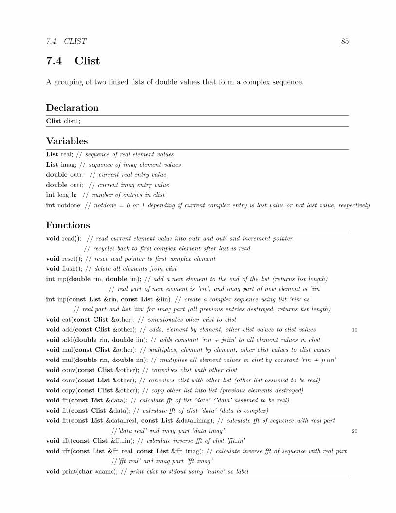
7.4. CLIST 85
7.4 Clist
A grouping of two linked lists of double values that form a complex sequence.
Declaration
Clist clist1;
Variables
List real; // sequence of real element values
List imag; // sequence of imag element values
double outr; // current real entry value
double outi; // current imag entry value
int length; // number of entries in clist
int notdone; // notdone = 0 or 1 depending if current complex entry is last value or not last value, respectively
Functions
void read(); // read current element value into outr and outi and increment pointer
// recycles back to first complex element after last is read
void reset(); // reset read pointer to first complex element
void flush(); // delete all elements from clist
int inp(double rin, double iin); // add a new element to the end of the list (returns list length)
// real part of new element is ’rin’, and imag part of new element is ’iin’
int inp(const List &rin, const List &iin); // create a complex sequence using list ’rin’ as
// real part and list ’iin’ for imag part (all previous entries destroyed, returns list length)
void cat(const Clist &other); // concatonates other clist to clist
void add(const Clist &other); // adds, element by element, other clist values to clist values 10
void add(double rin, double iin); // adds constant ’rin + j∗iin’ to all element values in clist
void mul(const Clist &other); // multiplies, element by element, other clist values to clist values
void mul(double rin, double iin); // multiplies all element values in clist by constant ’rin + j∗iin’void conv(const Clist &other); // convolves clist with other clist
void conv(const List &other); // convolves clist with other list (other list assumed to be real)
void copy(const Clist &other); // copy other list into list (previous elements destroyed)
void fft(const List &data); // calculate fft of list ’data’ (’data’ assumed to be real)
void fft(const Clist &data); // calculate fft of clist ’data’ (data is complex)
void fft(const List &data real, const List &data imag); // calculate fft of sequence with real part
//’data real’ and imag part ’data imag’ 20
void ifft(const Clist &fft in); // calculate inverse fft of clist ’fft in’
void ifft(const List &fft real, const List &fft imag); // calculate inverse fft of sequence with real part
//’fft real’ and imag part ’fft imag’
void print(char ∗name); // print clist to stdout using ’name’ as label

86 CHAPTER 7. GENERAL PURPOSE CPPSIM CLASSES
Example of Usage
#include "com_blocks.h"
main()
{// declarations
List list1,list2;
Clist clist1,clist2;
int i;
// incrementally load values into list1 10
list1.inp(1.0);
list1.inp(−1.0);
list1.inp(3.0);
list1.inp(5.0);
// incrementally load values into list2
list2.inp(3.0);
list2.inp(−4.0);
list2.inp(7.0);
list2.inp(5.0); 20
// create a complex list with list1 as real part, list2 as imag part
clist1.inp(list1,list2);
// copy clist1 to clist2
clist2.copy(clist1);
// change clist1 to its complex conjugate
clist1.imag.mul(−1.0);
30
// multiply elements of clist1 and clist2 and store in clist1 (clist2 unchanged)
clist1.mul(clist2);
// add elements of clist1 and clist2 and store in clist2 (clist1 unchanged)
clist2.add(clist1);
// multiply elements of clist2 by 1+j3
clist2.mul(1,3);
// add 2-j7 to elements of clist2 40

7.4. CLIST 87
clist2.add(2,−7);
// concatonate clist1 to clist2
clist2.cat(clist1);
// convolve clist1 and clist2 and place in clist2 (clist1 unchanged)
clist2.conv(clist1);
// compute the fft of clist2 and place in clist1 (clist2 unchanged)
clist1.fft(clist2); 50
// compute the ifft of clist1 and place back into clist1
clist1.ifft(clist1);
// compute the fft of list1 (assumed real) and place in clist2
clist2.fft(list1);
// delete all entries in clist2
clist2.flush();
// enter in new values 60
clist2.inp(1.0,2.0); // add element of value 1.0 + j2.0
clist2.inp(−1.0,3.0); // add element of value -1.0 + j3.0
clist2.inp(7.0,4.0); // add element of value 7.0 + j4.0
clist2.inp(5.0,1.0); // add element of value 5.0 + j
// illustrate read() by printing out entries of clist2 ‘by hand’
clist2.reset(); // resets read pointer to first complex entry
i = 1;
while(clist2.notdone)
{ 70
clist2.read(); // read current complex entry, increment pointer
printf("clist2[%d] = %5.3f + j%5.3f\n",i++,clist2.outr,clist2.outi);
}// illustrate recycling property of read() by reading beyond length of list
clist2.reset(); // resets read pointer to first complex entry
for (i = 1; i <= 20; i++) // will recycle through complex elements of clist2 many times
{clist2.read(); // read current complex entry, increment pointer
printf("clist2[%d] = %5.3f + j%5.3f\n",i,clist2.outr,clist2.outi);
} 80
// print out entries of clist2 using print function

88 CHAPTER 7. GENERAL PURPOSE CPPSIM CLASSES
clist2.print("clist2"); // character string serves as label for printout
// save values of clist2 to files
clist2.real.save("real.dat");
clist2.imag.save("imag.dat");
}

7.5. PROBE 89
7.5 Probe
Save data in single-precision format to a binary file which can be read with loadsig cppsim
in Matlab.
Declaration
Probe probe1("test.tr0"); // save probed data in file ’test.tr0’, sample period = 1
Probe probe2("test2.tr0",1e−6); // save probed data in file ’test2.tr0’, sample period = 1e-6
Probe probe3("test3.tr0",1e−6,10); // save probed data in file ’test3.tr0’, sample period = 1e-6
// subsample data by a factor of 10 before saving to file
Variables
None
Functions
void inp(double node value, char ∗node name); // send double value to probe file with label ’node name’
void inp(int int node value, char ∗node name); // send integer value to probe file with label ’node name’
Example of Usage
#include "com_blocks.h"
main()
{int i;
double Ts;
double sig1,sig2;
Ts = 1e−6;
Probe probe1("test.tr0"); 10
Probe probe2("test2.tr0",Ts);
Probe probe3("test3.tr0",Ts,10);
Probe probe4("test4.tr0",Ts);
for (i = 0; i < 1000; i++)
{sig1 = sin((2∗PI/200)∗i);sig2 = cos((2∗PI/200)∗i);// save signals to ’test.tr0’ with TIME signal in file having period = 1
probe1.inp(sig1,"sine"); 20
probe1.inp(sig2,"cosine");

90 CHAPTER 7. GENERAL PURPOSE CPPSIM CLASSES
// save signals to ’test2.tr0’ with TIME signal in file having period = Ts
probe2.inp(sig1,"sine");
probe2.inp(sig2,"cosine");
// save signals to ’test3.tr0’ with TIME signal in file having period = Ts
// and being subsampled by a factor of 10 (i.e. only 100 samples saved per signal in this case)
probe3.inp(sig1,"sine");
probe3.inp(sig2,"cosine");
}30
// Recommendation: don’t re-use probe statements in two different loops
for (i = 0; i < 1000; i++)
{sig1 = sin((2∗PI/250)∗i);sig2 = cos((2∗PI/250)∗i);// The following probe statements will produce an error
// probe1.inp(sig1,“sine2”); // don’t do this!
// probe1.inp(sig2,“cosine2”); // don’t do this!
// Probe statements used in previous loops must follow same order of signal names probed 40
probe2.inp(sig1,"sine"); // acceptable, but not recommended
probe2.inp(sig2,"cosine"); // acceptable, but not recommended
// probe2.inp(sig1+sig2,“sum”); // will produce an error since ’sum’ not probed in loop above
// The following probe statements are fine sinece probe4 was not used above
probe4.inp(sig1,"sine"); // recommended approach - new probe statement for this loop
probe4.inp(sig2,"cosine"); // ditto - this is fine
probe4.inp(sig1+sig2,"sum"); // ditto - this is fine
}} 50

7.6. PROBE64 91
7.6 Probe64
Save data in double-precision format to a binary file which can be read with loadsig cppsim
in Matlab.
Declaration
Probe64 probe1("test.tr0"); // save probed data in file ’test.tr0’, sample period = 1
Probe64 probe2("test2.tr0",1e−6); // save probed data in file ’test2.tr0’, sample period = 1e-6
Probe64 probe3("test3.tr0",1e−6,10); // save probed data in file ’test3.tr0’, sample period = 1e-6
// subsample data by a factor of 10 before saving to file
Variables
None
Functions
void inp(double node value, char ∗node name); // send double value to probe file with label ’node name’
void inp(int int node value, char ∗node name); // send integer value to probe file with label ’node name’
Example of Usage
#include "com_blocks.h"
main()
{int i;
double Ts;
double sig1,sig2;
Ts = 1e−6;
Probe64 probe1("test.tr0"); 10
Probe64 probe2("test2.tr0",Ts);
Probe64 probe3("test3.tr0",Ts,10);
Probe64 probe4("test4.tr0",Ts);
for (i = 0; i < 1000; i++)
{sig1 = sin((2∗PI/200)∗i);sig2 = cos((2∗PI/200)∗i);// save signals to ’test.tr0’ with TIME signal in file having period = 1
probe1.inp(sig1,"sine"); 20
probe1.inp(sig2,"cosine");

92 CHAPTER 7. GENERAL PURPOSE CPPSIM CLASSES
// save signals to ’test2.tr0’ with TIME signal in file having period = Ts
probe2.inp(sig1,"sine");
probe2.inp(sig2,"cosine");
// save signals to ’test3.tr0’ with TIME signal in file having period = Ts
// and being subsampled by a factor of 10 (i.e. only 100 samples saved per signal in this case)
probe3.inp(sig1,"sine");
probe3.inp(sig2,"cosine");
}30
// Recommendation: don’t re-use probe statements in two different loops
for (i = 0; i < 1000; i++)
{sig1 = sin((2∗PI/250)∗i);sig2 = cos((2∗PI/250)∗i);// The following probe statements will produce an error
// probe1.inp(sig1,“sine2”); // don’t do this!
// probe1.inp(sig2,“cosine2”); // don’t do this!
// Probe statements used in previous loops must follow same order of signal names probed 40
probe2.inp(sig1,"sine"); // acceptable, but not recommended
probe2.inp(sig2,"cosine"); // acceptable, but not recommended
// probe2.inp(sig1+sig2,“sum”); // will produce an error since ’sum’ not probed in loop above
// The following probe statements are fine sinece probe4 was not used above
probe4.inp(sig1,"sine"); // recommended approach - new probe statement for this loop
probe4.inp(sig2,"cosine"); // ditto - this is fine
probe4.inp(sig1+sig2,"sum"); // ditto - this is fine
}} 50

7.7. FILTER 93
7.7 Filter
Continuous-time and discrete-time filters.
Declaration
Filter difference("1 - z^-1","1"); // discrete-time first difference
Filter accum("1","1 - z^-1"); // discrete-time accumulator
Filter zfilt("1 - a*z^-1","1 - b*z^-1","a,b",.8,.9); // general discrete-time
// filter consisting of one pole and one zero
Filter accum lim("1","1 - z^-1","Max,Min",2.5,0.0); // discrete-time accumulator
// with max and min limits set on its output
Filter delay("z^-no","1","no",10); // delay of 10 samples (must use integer sample delay)
Filter diff("K*s","1","Ts,K",1e−6,2.0); // continuous-time differentiator K∗s// (Ts is simulation sample period)
Filter integ("K","s","K,Ts",1,1e−6); // continuous-time integrator K/s 10
Filter RC fil("K","1 + 1/(2*pi*fo)*s","K,fo,Ts",1.0,1e3,1e−6); // continuous-time filter
// corresponding to an RC network with transfer function K/(1 + s/(2∗pi∗fo))Filter LC fil("K","1 + 1/(wo*Q)*s + 1/(wo^2)*s^2","Ts,K,wo,Q",1e−6,1.0,1e3∗2∗PI,1.2);
// continuous-time filter corresponding to an LC network with
// transfer function K/(1 + 1/(wo∗Q)∗s + (s/wo)^2)
List list1;
list1.load("list1.dat"); // load data from file into list
Filter(list1,"1"); // create z-domain FIR filter whose numerator z-polynomial is created from
// list1 elements and whose denominator is 1 (see Usage example below)
Filter("1",list1); // create z-domain IIR filter whose denominator z-polynomial is created from 20
// list1 elements and whose numerator is 1
List list2;
list2.load("list2.dat");
Filter(list1,list2); // create z-domain IIR filter whose denominator z-polynomial is created from
// list1 elements and whose numerator z-polynomial is created from list2 elements
Vector vec1;
vec1.load("list1.dat"); // load data from file into real-valued vector
Filter(vec1,"1"); // create z-domain FIR filter whose numerator z-polynomial is created from
// vec1 elements and whose denominator is 1
Redefinition (this is rarely required)
// Declaration
Filter filt1("1 - z^-1","1");
// Redefine

94 CHAPTER 7. GENERAL PURPOSE CPPSIM CLASSES
filt1.set("1","1 - z^-1");
// Redefine again
filt1.set("K","1 + 1/(2*pi*fo)*s","K,fo,Ts",1.0,1e3,1e−6);
Variables
double out; // output of filter
char ivar; // independent variable of transfer function - either ’z’ or ’s’
int num a coeff; // number of denominator coefficients
int num b coeff; // number of numerator coefficients
Functions
double inp(double in); // input new sample to filter, resulting output is returned
void reset(double value); // set output and all state information of filter to value
Example of Usage
#include "com_blocks.h"
main()
{List list1;
Probe probe1("test.tr0");
int i;
double in;
// incrementally load values into list1 to later set z-polynomial of a0 + a1∗z^-1 + a2∗z^-2 10
list1.inp(1.0); // set a0
list1.inp(−2.0); // set a1
list1.inp(1.0); // set a2
/////////////////// discrete-time filter implementation //////////////////////
// create two filters (cascade of which is an accumulator)
Filter double accum("1",list1);
Filter first diff("1 - z^-1","1");
in = 1.0; 20
for (i = 0; i < 1000; i++)
{if (i == 200)
in = −1.0;
else if (i == 400)
in = 2.0;

7.7. FILTER 95
else if (i == 700) // zero out filters at the 700th sample
{double accum.reset(0.0);
first diff.reset(0.0); 30
}
// cascade the filters
double accum.inp(in);
first diff.inp(double accum.out);
// save the signals to file ’test.tr0’ using probe1
probe1.inp(in,"in");
probe1.inp(double accum.out,"accum2");
probe1.inp(first diff.out,"accum1"); 40
}
/////////////////// continuous-time filter implementation //////////////////////
double sample per;
sample per = 1e−6; // choose 1 us sample period
Probe probe2("test2.tr0",sample per); // need a new probe statement for new iteration loop
// create two filters (cascade of which is an integrator)
Filter double integ("K","s^2","K,Ts",1e5,sample per); 50
Filter diff("s","1","Ts",sample per);
in = 1.0;
for (i = 0; i < 1000; i++)
{if (i == 200)
in = −1.0;
else if (i == 400)
in = 2.0;
else if (i == 700) // zero out filters at the 700th sample 60
{double integ.reset(0.0);
diff.reset(0.0);
}
// cascade the filters
double integ.inp(in);

96 CHAPTER 7. GENERAL PURPOSE CPPSIM CLASSES
diff.inp(double integ.out);
// save the signals to file ’test2.tr0’ using probe2 70
probe2.inp(in,"in");
probe2.inp(double integ.out,"int2");
probe2.inp(diff.out,"int1");
}}

7.8. AMP 97
7.8 Amp
General amplifier with nonlinear characteristic specified by a polynomial and saturating
characteristic specified by Min, Max values.
Declaration
Amp amp("off + A*x","off,A",1.0,5.0); // amp offset of 1 V, gain of 5
Amp amp2("off + A*x + A1*x^2 + A2*x^(1/2)","off,A,A1,A2",.5,10.0,1,.1); // nonlinear
// characterstic described by a polynmomial
Amp amp("off + A*x","off,A,Min,Max",1.0,5.0,0.5,2.0); // Min output is 0.5, Max output is 2.0
Redefinition (this is rarely required)
// Declaration
Amp amp("off + A*x","off,A",1.0,5.0); // amp offset of 1 V, gain of 5
// Redefine
amp.set("off + A*x + A1*x^2 + A2*x^(1/2)","off,A,A1,A2",.5,10.0,1,.1);
// Redefine again
amp.set("off + A*x","off,A,Min,Max",1.0,5.0,0.5,2.0);
Variables
double out; // output of amplifier
Functions
double inp(double in); // input voltage to amp, returns resulting value of out
Example of Usage
#include "com_blocks.h"
main()
{int i;
double Ts;
double in;
Ts = 1e−6;
Probe probe1("test.tr0",Ts); 10
// create an amplifier with offset -0.5, gain 3.0, and saturation at 0 (min) and 2.0 (max)
Amp amp1("off + A*x","off,A,Max,Min",−0.5,3.0,2.0,0.0);

98 CHAPTER 7. GENERAL PURPOSE CPPSIM CLASSES
for (i = 0; i < 1000; i++)
{in = (1.0/1000.0)∗i;amp1.inp(in); // input ramped from 0 to 1
probe1.inp(in,"in"); // save input of amp
probe1.inp(amp1.out,"out"); // save output of amp
} 20
}
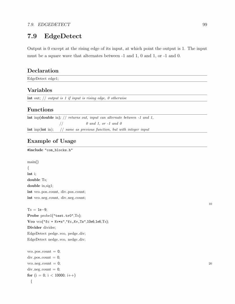
7.9. EDGEDETECT 99
7.9 EdgeDetect
Output is 0 except at the rising edge of its input, at which point the output is 1. The input
must be a square wave that alternates between -1 and 1, 0 and 1, or -1 and 0.
Declaration
EdgeDetect edge1;
Variables
int out; // output is 1 if input is rising edge, 0 otherwise
Functions
int inp(double in); // returns out, input can alternate between -1 and 1,
// 0 and 1, or -1 and 0
int inp(int in); // same as previous function, but with integer input
Example of Usage
#include "com_blocks.h"
main()
{int i;
double Ts;
double in,sig1;
int vco pos count, div pos count;
int vco neg count, div neg count;
10
Ts = 1e−9;
Probe probe1("test.tr0",Ts);
Vco vco("fc + Kv*x","fc,Kv,Ts",10e6,1e6,Ts);
Divider divider;
EdgeDetect pedge vco, pedge div;
EdgeDetect nedge vco, nedge div;
vco pos count = 0;
div pos count = 0;
vco neg count = 0; 20
div neg count = 0;
for (i = 0; i < 10000; i++)
{

100 CHAPTER 7. GENERAL PURPOSE CPPSIM CLASSES
in = (1.0/10000.0)∗i;vco.inp(in); // frequency will gradually increase since in is a ramp
divider.inp(vco.out,10.0); // divide down VCO frequency by a factor of 10
if (pedge vco.inp(vco.out)) // count rising edges of VCO
vco pos count++;
if (nedge vco.inp(−vco.out)) // count falling edges of VCO 30
vco neg count++;
if (pedge div.inp(divider.out)) // count rising edges of divider output
div pos count++;
// don’t do the following: (edge module cannot be used twice in one loop)
// if (pedge div.inp(-divider.out)) // count falling edges of divider output
// div pos count++;
// instead, use a distinct edge module:
if (nedge div.inp(−divider.out)) // count falling edges of divider output
div neg count++;
40
probe1.inp(vco.out,"vco"); // save square wave output of VCO
probe1.inp(divider.out,"divide"); // save square wave output of divider
}printf("vco_pos_count = %d, div_pos_count = %d\n",vco pos count,div pos count);
printf("vco_neg_count = %d, div_neg_count = %d\n",vco neg count,div neg count);
}

7.10. SDMBITMOD 101
7.10 SdMbitMod
Implements a multi-bit Σ-Δ modulator with a signal transfer function (STF) of 1.0 and a
noise transfer function (NTF) that is specified as a z polynomial.
Declaration
SdMbitMod sd mod1("1 - 2*z^-1 + z^-2"); // sd modulator with second order noise shaping
SdMbitMod sd mod2("1 - 3z^-1 + 3z^-2 - 1z^-3"); // sd modulator with third order noise shaping
Redefinition (this is rarely required)
// Declaration
SdMbitMod sd mod1("1 - 2*z^-1 + z^-2");
// Redefine
sd mod1.set("1 - 3z^-1 + 3z^-2 - 1z^-3");
// Redefine again
sd mod1.set("1 - z^-1");
Variables
double out; // output of sd modulator
Functions
double inp(double in); // returns sd modulator ’out’ given input ’in’
Example of Usage
#include "com_blocks.h"
main()
{int i;
double Ts;
double in;
Ts = 1e−9;
Probe probe1("test.tr0",Ts); 10
Filter lowpass("1","1 + 1/(2*pi*fo)*s","fo,Ts",100e3,Ts);
SdMbitMod sdmod("1 - 2z^-1 + z^-2");

102 CHAPTER 7. GENERAL PURPOSE CPPSIM CLASSES
for (i = 0; i < 10000; i++)
{in = sin(2∗pi∗50e3∗Ts∗i); // create a sine wave for input to the sd modulator
sdmod.inp(in); // input the sine wave into the sd modulator
lowpass.inp(sdmod.out); // filter the sd modulator output
20
probe1.inp(in,"in"); // save input sine wave
probe1.inp(sdmod.out,"sdmod"); // save output of sd modulator
probe1.inp(lowpass.out,"out"); // save output of lowpass
}}
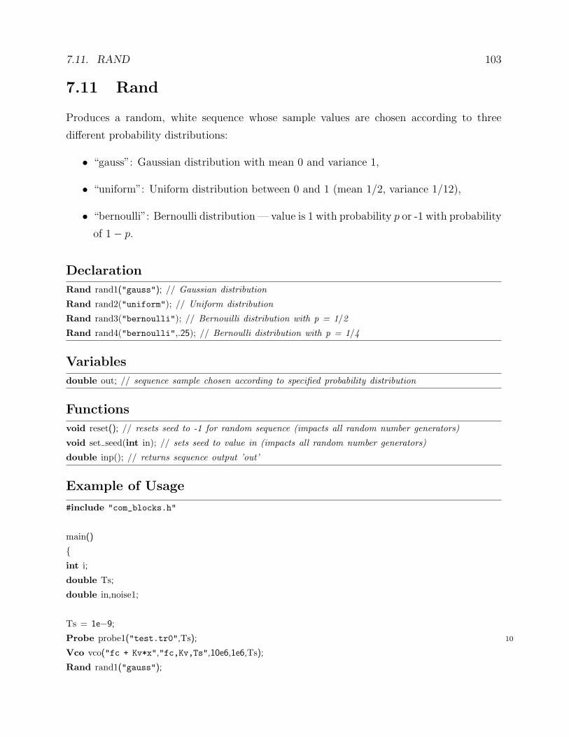
7.11. RAND 103
7.11 Rand
Produces a random, white sequence whose sample values are chosen according to three
different probability distributions:
• “gauss”: Gaussian distribution with mean 0 and variance 1,
• “uniform”: Uniform distribution between 0 and 1 (mean 1/2, variance 1/12),
• “bernoulli”: Bernoulli distribution — value is 1 with probability p or -1 with probability
of 1− p.
Declaration
Rand rand1("gauss"); // Gaussian distribution
Rand rand2("uniform"); // Uniform distribution
Rand rand3("bernoulli"); // Bernouilli distribution with p = 1/2
Rand rand4("bernoulli",.25); // Bernoulli distribution with p = 1/4
Variables
double out; // sequence sample chosen according to specified probability distribution
Functions
void reset(); // resets seed to -1 for random sequence (impacts all random number generators)
void set seed(int in); // sets seed to value in (impacts all random number generators)
double inp(); // returns sequence output ’out’
Example of Usage
#include "com_blocks.h"
main()
{int i;
double Ts;
double in,noise1;
Ts = 1e−9;
Probe probe1("test.tr0",Ts); 10
Vco vco("fc + Kv*x","fc,Kv,Ts",10e6,1e6,Ts);
Rand rand1("gauss");

104 CHAPTER 7. GENERAL PURPOSE CPPSIM CLASSES
for (i = 0; i < 10000; i++)
{if (i == 5000) // reset random sequence at i = 5000
rand1.reset();
if (i == 7000) // change seed value of random sequence at i = 7000
rand1.set seed(−2);
20
in = (1.0/10000.0)∗i; // create a ramp signal
noise1 = .01∗rand1.inp() + 0.2; // gaussian sequence with mean 0.2, variance (.01)^2
vco.inp(in+noise1); // add noise to input signal to VCO
probe1.inp(in+noise1,"in"); // save input to VCO
probe1.inp(noise1,"noise"); // save noise sequence
probe1.inp(vco.out,"vco"); // save square wave output of VCO
}}
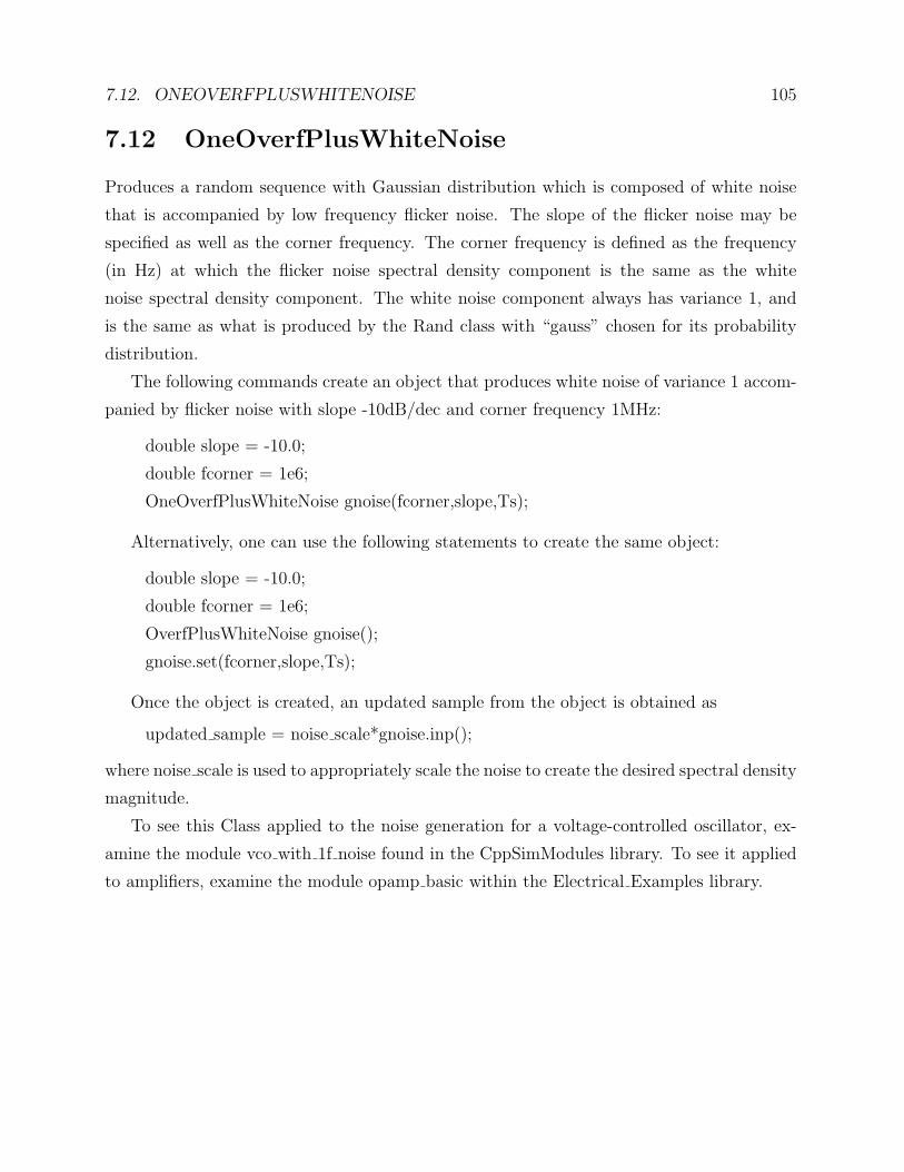
7.12. ONEOVERFPLUSWHITENOISE 105
7.12 OneOverfPlusWhiteNoise
Produces a random sequence with Gaussian distribution which is composed of white noise
that is accompanied by low frequency flicker noise. The slope of the flicker noise may be
specified as well as the corner frequency. The corner frequency is defined as the frequency
(in Hz) at which the flicker noise spectral density component is the same as the white
noise spectral density component. The white noise component always has variance 1, and
is the same as what is produced by the Rand class with “gauss” chosen for its probability
distribution.
The following commands create an object that produces white noise of variance 1 accom-
panied by flicker noise with slope -10dB/dec and corner frequency 1MHz:
double slope = -10.0;
double fcorner = 1e6;
OneOverfPlusWhiteNoise gnoise(fcorner,slope,Ts);
Alternatively, one can use the following statements to create the same object:
double slope = -10.0;
double fcorner = 1e6;
OverfPlusWhiteNoise gnoise();
gnoise.set(fcorner,slope,Ts);
Once the object is created, an updated sample from the object is obtained as
updated sample = noise scale*gnoise.inp();
where noise scale is used to appropriately scale the noise to create the desired spectral density
magnitude.
To see this Class applied to the noise generation for a voltage-controlled oscillator, ex-
amine the module vco with 1f noise found in the CppSimModules library. To see it applied
to amplifiers, examine the module opamp basic within the Electrical Examples library.

106 CHAPTER 7. GENERAL PURPOSE CPPSIM CLASSES
7.13 Quantizer
Quantizes input according to five parameters: levels, step size, in center, out min, and
out max as shown in Figure 7.1
0
in
0
out
t
t
in_center step_size
levels=5
out_min
out_max
0
in
0
out
t
t
in_centerstep_size
levels=4
out_min
out_max
Figure 7.1 Illustration of behavior of Quantizer class in relation to parameter settings.
Declaration
Quantizer quant1(2,.5,0.0,−1,1); // levels=2, step size=0.5, in center=0, out min=-1, out max=1
Quantizer quant2(2,.5,0.5,−1,1);
Quantizer quant3(2,.5,−0.5,0,1);
Quantizer quant4(3,.5,0.0,−1,1);
Quantizer quant5(5,.5,0.0,−1,1);
Quantizer quant6(5,.5,0.0,0,4);
Quantizer quant7(16,.3,0.0,0,15);
Variables
double out; // output of quantizer
Functions
double inp(double in); // returns quantized out for given in
double inp(double in, double clk); // returns quantized out for given in on rising edge of clk
Example of Usage
#include "com_blocks.h"

7.13. QUANTIZER 107
main()
{double Ts=1;
Quantizer quant1(2,.5,0.0,−1,1);
Quantizer quant2(2,.5,0.5,−1,1);
Quantizer quant3(2,.5,−0.5,0,1);
Quantizer quant4(3,.5,0.0,−1,1);
Quantizer quant5(5,.5,0.0,−1,1); 10
Quantizer quant6(5,.5,0.0,0,4);
Quantizer quant7(16,.3,0.0,0,15);
Vco vco("fc + Kv*x","Ts,fc,Kv",Ts,1/150.0,1.0);
Probe probe1("test.tr0");
double in;
int i;
in = −2.0;
for (i = 0; i < 4000; i++)
{ 20
// generate input signal
if (i % 2000 < 1000)
in += .004;
else
in −= .004;
// clockless quantizer examples
quant1.inp(in);
quant2.inp(in);
quant3.inp(in); 30
quant4.inp(in);
quant5.inp(in);
quant6.inp(in);
// clocked quantizer examples
vco.inp(0.0);
quant7.inp(in,vco.out);
// save signals to file
probe1.inp(in,"in"); 40
probe1.inp(vco.out,"clk");
probe1.inp(quant1.out,"quant1");
probe1.inp(quant2.out,"quant2");

108 CHAPTER 7. GENERAL PURPOSE CPPSIM CLASSES
probe1.inp(quant3.out,"quant3");
probe1.inp(quant4.out,"quant4");
probe1.inp(quant5.out,"quant5");
probe1.inp(quant6.out,"quant6");
probe1.inp(quant7.out,"quant7");
}} 50
0 500 1000 1500 2000 2500 3000 3500 4000−2
−1
0
1
2
in,q
uant
1
0 500 1000 1500 2000 2500 3000 3500 4000−2
−1
0
1
2
in,q
uant
2
0 500 1000 1500 2000 2500 3000 3500 4000−2
−1
0
1
2
in,q
uant
3
TIME
Figure 7.2 Plot of quant1, quant2, and quant3 from example simulation.

7.13. QUANTIZER 109
0 500 1000 1500 2000 2500 3000 3500 4000−2
−1
0
1
2
in,q
uant
4
0 500 1000 1500 2000 2500 3000 3500 4000−2
−1
0
1
2
in,q
uant
5
0 500 1000 1500 2000 2500 3000 3500 4000−2
0
2
4
in,q
uant
6
TIME
Figure 7.3 Plot of quant4, quant5, and quant6 from example simulation.
0 500 1000 1500 2000 2500 3000 3500 4000−2
−1
0
1
2
in
0 500 1000 1500 2000 2500 3000 3500 4000−1
−0.5
0
0.5
1
clk
0 500 1000 1500 2000 2500 3000 3500 40000
5
10
15
quan
t7
TIME
Figure 7.4 Plot of quant7 and associated signals from example simulation.

110 CHAPTER 7. GENERAL PURPOSE CPPSIM CLASSES

Chapter 8
CppSim Classes for PLL/DLL
Simulation
These classes are used in the same manner as the general purpose ones described in the
previous chapter, but are specialized for PLL/DLL simulation in that they implement the
area conservation approach for digital signal transitions that is described in the paper
Perrott, M.H., “Fast and Accurate Behavioral Simulation of
Fractional-N Frequency Synthesizers and other PLL/DLL Circuits,”
Design Automation Conference, June, 2002
An expanded version of the above paper is included in the CppSim package — the included
version more explicitly relates the described techniques to the classes provided in this library.
111

112 CHAPTER 8. CPPSIM CLASSES FOR PLL/DLL SIMULATION
8.1 SigGen
Produces a waveform of a specified frequency that corresponds to one of four different wave-
form types:
• “square”: a square wave (alternating between 1 and -1),
• “sine”: a sine wave (amplitude 1, DC offset 0),
• “prbs”: a prbs data sequence (alternating between 1 and -1),
• “impulse”: an impulse data sequence.
Declaration
double Ts=1e−9; // simulation sample period
SigGen siggen1("square",1.0e6,Ts); //square wave of frequency 1 MHz
SigGen siggen2("sine",1.0e6,Ts); // sine wave of frequency 1 MHz
SigGen siggen3("prbs",1.0e6,Ts); // prbs sequence of period 1/(1 MHz), data chosen randomly
List list1;
list1.load("list1.dat"); // load data sequence from file, which must have values of either 1 or -1
SigGen siggen4("prbs",1.0e6,Ts,list1); // prbs sequence of period 1/(1 MHz), data repeats through list1
SigGen siggen4("prbs",1.0e6,Ts,list1,5); // prbs sequence of period 1/(1 MHz),
// data repeats through list1, start with 5th entry in list
SigGen siggen5("impulse",1.0e6,Ts); // impulse sequence of period 1/(1 MHz), data chosen randomly 10
SigGen siggen6("impulse",1.0e6,Ts,list1); // impulse sequence of period 1/(1 MHz), data repeats through list1
SigGen siggen6("impulse",1.0e6,Ts,list1,3); // impulse sequence of period 1/(1 MHz),
// data repeats through list1, start with 3rd entry in list
Redefinition (this is rarely required)
// Declaration
SigGen siggen1("square",1.0e6,Ts);
// Redefine
siggen1.set("sine",1.0e6,Ts);
// Redefine again
siggen1.set("prbs",1.0e6,Ts);
Variables
double out; // waveform output
double phase; // normalized phase of waveform (ramps between 0.0 and 1.0)
double square; // square wave (clk) that output is derived from
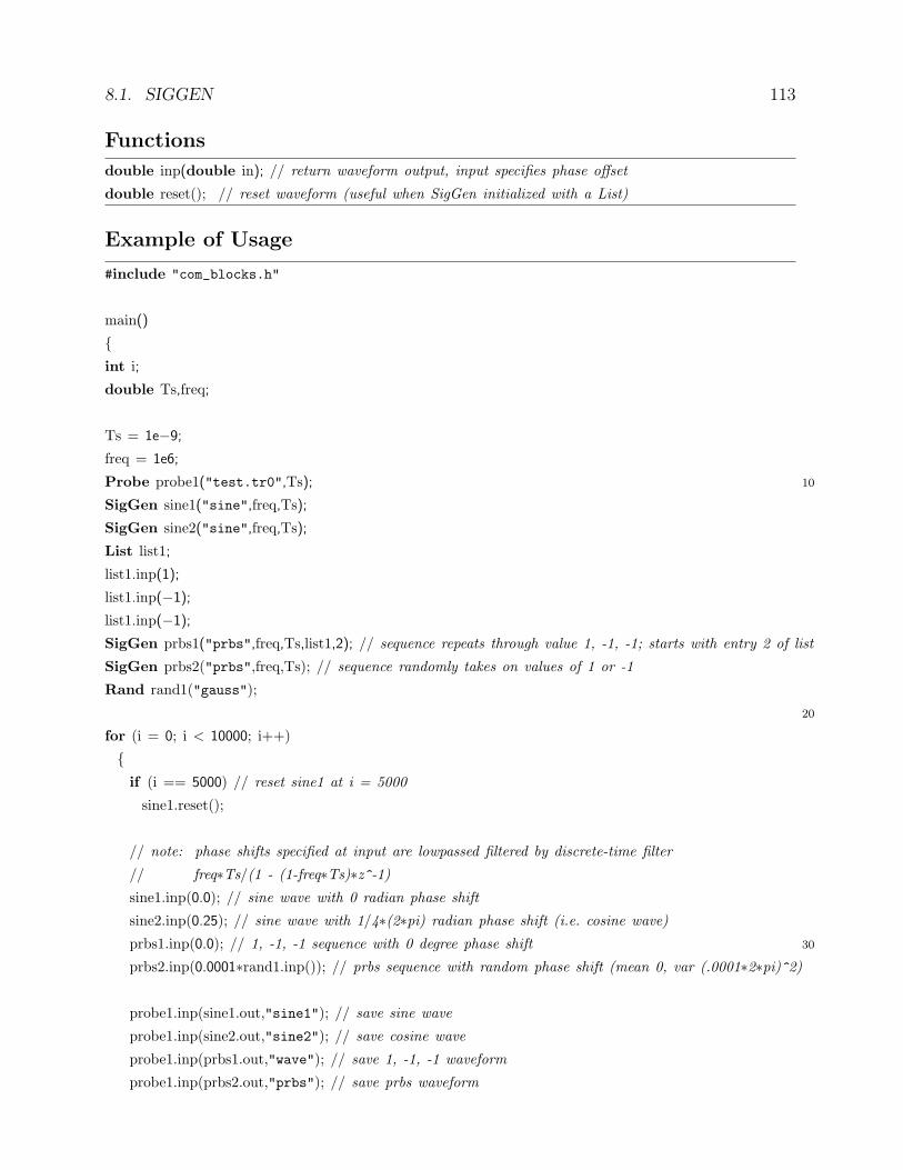
8.1. SIGGEN 113
Functions
double inp(double in); // return waveform output, input specifies phase offset
double reset(); // reset waveform (useful when SigGen initialized with a List)
Example of Usage
#include "com_blocks.h"
main()
{int i;
double Ts,freq;
Ts = 1e−9;
freq = 1e6;
Probe probe1("test.tr0",Ts); 10
SigGen sine1("sine",freq,Ts);
SigGen sine2("sine",freq,Ts);
List list1;
list1.inp(1);
list1.inp(−1);
list1.inp(−1);
SigGen prbs1("prbs",freq,Ts,list1,2); // sequence repeats through value 1, -1, -1; starts with entry 2 of list
SigGen prbs2("prbs",freq,Ts); // sequence randomly takes on values of 1 or -1
Rand rand1("gauss");
20
for (i = 0; i < 10000; i++)
{if (i == 5000) // reset sine1 at i = 5000
sine1.reset();
// note: phase shifts specified at input are lowpassed filtered by discrete-time filter
// freq∗Ts/(1 - (1-freq∗Ts)∗z^-1)sine1.inp(0.0); // sine wave with 0 radian phase shift
sine2.inp(0.25); // sine wave with 1/4∗(2∗pi) radian phase shift (i.e. cosine wave)
prbs1.inp(0.0); // 1, -1, -1 sequence with 0 degree phase shift 30
prbs2.inp(0.0001∗rand1.inp()); // prbs sequence with random phase shift (mean 0, var (.0001∗2∗pi)^2)
probe1.inp(sine1.out,"sine1"); // save sine wave
probe1.inp(sine2.out,"sine2"); // save cosine wave
probe1.inp(prbs1.out,"wave"); // save 1, -1, -1 waveform
probe1.inp(prbs2.out,"prbs"); // save prbs waveform

114 CHAPTER 8. CPPSIM CLASSES FOR PLL/DLL SIMULATION
}}
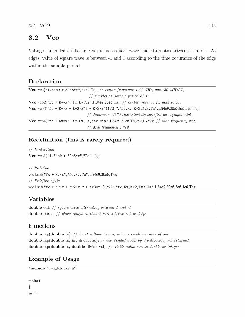
8.2. VCO 115
8.2 Vco
Voltage controlled oscillator. Output is a square wave that alternates between -1 and 1. At
edges, value of square wave is between -1 and 1 according to the time occurance of the edge
within the sample period.
Declaration
Vco vco("1.84e9 + 30e6*x","Ts",Ts); // center frequency 1.84 GHz, gain 30 MHz/V,
// simulation sample period of Ts
Vco vco2("fc + Kv*x","fc,Kv,Ts",1.84e9,30e6,Ts); // center freqency fc, gain of Kv
Vco vco3("fc + Kv*x + Kv2*x^2 + Kv3*x^(1/2)","fc,Kv,Kv2,Kv3,Ts",1.84e9,30e6,5e6,1e6,Ts);
// Nonlinear VCO characteristic specified by a polynomial
Vco vco4("fc + Kv*x","fc,Kv,Ts,Max,Min",1.84e9,30e6,Ts,2e9,1.7e9); // Max frequency 2e9,
// Min frequency 1.7e9
Redefinition (this is rarely required)
// Declaration
Vco vco1("1.84e9 + 30e6*x","Ts",Ts);
// Redefine
vco1.set("fc + Kv*x","fc,Kv,Ts",1.84e9,30e6,Ts);
// Redefine again
vco1.set("fc + Kv*x + Kv2*x^2 + Kv3*x^(1/2)","fc,Kv,Kv2,Kv3,Ts",1.84e9,30e6,5e6,1e6,Ts);
Variables
double out; // square wave alternating between 1 and -1
double phase; // phase wraps so that it varies between 0 and 2pi
Functions
double inp(double in); // input voltage to vco, returns resulting value of out
double inp(double in, int divide val); // vco divided down by divide value, out returned
double inp(double in, double divide val); // divide value can be double or integer
Example of Usage
#include "com_blocks.h"
main()
{int i;

116 CHAPTER 8. CPPSIM CLASSES FOR PLL/DLL SIMULATION
double Ts;
double in,sig1;
Ts = 1e−9;
Probe probe1("test.tr0",Ts); 10
Vco vco("fc + Kv*x","fc,Kv,Ts",10e6,1e6,Ts);
Vco vco2("fc + Kv*x","fc,Kv,Ts",10e6,1e6,Ts);
for (i = 0; i < 10000; i++)
{in = (1.0/10000.0)∗i;vco.inp(in); // frequency will gradually increase since in is a ramp
vco2.inp(in,3); // divide vco output down in frequency by a factor of 3
sig1 = sin(vco.phase); // sine wave output from VCO instead of square wave
20
probe1.inp(vco.out,"square"); // save square wave output
probe1.inp(vco2.out,"square3"); // save square wave output divided by 3
probe1.inp(sig1,"sine"); // save sine wave output
}}
8.3. DELAY 117
8.3 Delay
Variable delay element for inputs that follow the interpolation convention (i.e. they must
alternate between -1.0 and 1.0, with transition values taking on a value in the range of -1.0
to 1.0 depending on the location of the transition relative to the sample period). Output
alternates between -1.0 and 1.0, with edge values between -1.0 and 1.0 according to their
actual time position within the sample period.
Declaration
Delay delay1(5.4); // nominal delay of 5.4 simulator time samples when varying delay
Delay delay2(3.6); // fixed delay of 3.6 simulator time samples for fixed delay
Variables
double out; // output of delay element (alternates between 1.0 and -1.0)
Functions
double inp(double in); // input ’in’ signal to delay, keep the delay value fixed
double inp(double in, double delay val); // adjust delay value about
// nominal value according to ’delay val’ signal
Example of Usage
118 CHAPTER 8. CPPSIM CLASSES FOR PLL/DLL SIMULATION
8.4 Divider
Divides down input square wave (which much alternate between -1 and 1) according to a
specified divide value. Output also alternates between -1 and 1.
Declaration
Divider divider1;
Variables
double out; // output square wave alternating between 1 and -1
Functions
double inp(double in, int divide value); // returns output given specified input and divide value
double inp(double in, double divide value); // divide value can be double or integer valued
Example of Usage
#include "com_blocks.h"
main()
{int i;
double Ts;
double in,sig1;
Ts = 1e−9;
Probe probe1("test.tr0",Ts); 10
Vco vco("fc + Kv*x","fc,Kv,Ts",10e6,1e6,Ts);
Divider divider;
for (i = 0; i < 10000; i++)
{in = (1.0/10000.0)∗i;vco.inp(in); // frequency will gradually increase since in is a ramp
divider.inp(vco.out,10.0); // divide down VCO frequency by a factor of 10
probe1.inp(vco.out,"vco"); // save square wave output of VCO 20
probe1.inp(divider.out,"divide"); // save square wave output of divider
}}

8.5. LATCH 119
8.5 Latch
Performs latch function with input, clock, set and reset that alternate between -1 and 1.
Declaration
Latch latch1;
Variables
double out; // output is 1 or -1 depending on latch state
Functions
// for all functions, in, clock, set, reset must be -1 or 1, values between -1 and 1 correspond to transitions
double inp(double in, double clk); // returns out based on in and clk
double inp(double in, double clk, double set, double reset); // includes set and reset
void init(double in); // initializes latch to value in (must be -1 or 1)
Example of Usage
#include "com_blocks.h"
main()
{int i;
double Ts;
double in,sig1;
Ts = 1e−9;
Probe probe1("test.tr0",Ts); 10
Vco vco("fc + Kv*x","fc,Kv,Ts",10e6,1e6,Ts);
Divider divider;
Latch latch1, latch2, latch3, latch4;
for (i = 0; i < 10000; i++)
{in = (1.0/10000.0)∗i;vco.inp(in); // frequency will gradually increase since in is a ramp
divider.inp(vco.out,10.0); // divide down VCO frequency by a factor of 10
20
// implement a register with divider output as its input, VCO output as its clock
latch1.inp(divider.out,vco.out); // first latch of register
latch2.inp(latch1.out,−vco.out); // second latch of register; note clk is inverted

120 CHAPTER 8. CPPSIM CLASSES FOR PLL/DLL SIMULATION
// implement a register with divider output as its input, VCO output as its clock
// reset the register according to above register output
latch3.inp(divider.out,vco.out,−1.0,latch2.out); // first latch of register
latch4.inp(latch3.out,−vco.out,−1.0,latch2.out); // second latch of register
probe1.inp(vco.out,"vco"); // save square wave output of VCO 30
probe1.inp(divider.out,"divide"); // save square wave output of divider
probe1.inp(latch2.out,"reg1"); // save output of register 1
probe1.inp(latch4.out,"reg2"); // save output of register 2
}}

8.6. REG 121
8.6 Reg
Performs register function with input, clock, set and reset that alternate between -1 and 1.
Declaration
Reg reg1;
Variables
double out; // output is 1 or -1 depending on register state
Latch lat1; // first latch in register
Latch lat2; // second latch in register
Functions
// for all functions, in, clock, set, reset must be -1 or 1, values between -1 and 1 correspond to transitions
double inp(double in, double clk); // returns out based on in and clk
double inp(double in, double clk, double set, double reset); // includes set and reset
void init(double in); // initializes both register latches to value in (must be -1 or 1)
Example of Usage
#include "com_blocks.h"
main()
{int i;
double Ts;
double in,sig1;
Ts = 1e−9;
Probe probe1("test.tr0",Ts); 10
Vco vco("fc + Kv*x","fc,Kv,Ts",10e6,1e6,Ts);
Divider divider;
Reg reg1, reg2;
for (i = 0; i < 10000; i++)
{in = (1.0/10000.0)∗i;vco.inp(in); // frequency will gradually increase since in is a ramp
divider.inp(vco.out,10.0); // divide down VCO frequency by a factor of 10
20
// implement a register with divider output as its input, VCO output as its clock

122 CHAPTER 8. CPPSIM CLASSES FOR PLL/DLL SIMULATION
reg1.inp(divider.out,vco.out);
// implement a register with divider output as its input, VCO output as its clock
// reset the register according to above register output
reg2.inp(divider.out,vco.out,−1.0,reg1.out);
probe1.inp(vco.out,"vco"); // save square wave output of VCO
probe1.inp(divider.out,"divide"); // save square wave output of divider
probe1.inp(reg1.out,"reg1"); // save output of register 1 30
probe1.inp(reg2.out,"reg2"); // save output of register 2
probe1.inp(reg1.lat1.out,"lat1"); // save output of lat1 of register 1
probe1.inp(reg2.lat1.out,"lat2"); // save output of lat1 of register 2
}}

8.7. XOR 123
8.7 Xor
Performs ‘xor’ function with 2 inputs that alternate between -1 and 1.
Declaration
Xor xor1;
Variables
double out; // output is 1 or -1 depending on xor of inputs
Functions
// inputs must be either -1 or 1
// values between -1 and 1 correspond to transitions
double inp(double in0, double in1); // returns out = -in0∗in1; (the xor function)
Example of Usage
#include "com_blocks.h"
main()
{int i;
double Ts;
double in,sig1;
Ts = 1e−9;
Probe probe1("test.tr0",Ts); 10
Vco vco("fc + Kv*x","fc,Kv,Ts",10e6,1e6,Ts);
Divider divider;
Reg reg1;
Xor xor1, xor2, xor3;
for (i = 0; i < 10000; i++)
{in = (1.0/10000.0)∗i;vco.inp(in); // frequency will gradually increase since in is a ramp
divider.inp(vco.out,10.0); // divide down VCO frequency by a factor of 10 20
reg1.inp(divider.out,vco.out); // register divider output with VCO output as clk
xor1.inp(divider.out,reg1.out); // xor divider out and reg1 out
124 CHAPTER 8. CPPSIM CLASSES FOR PLL/DLL SIMULATION
xor2.inp(−divider.out,reg1.out); // xor not(divider out) and reg1 out
xor3.inp(divider.out,−reg1.out); // xor divider out and not(reg1 out)
probe1.inp(vco.out,"vco"); // save square wave output of VCO
probe1.inp(divider.out,"divide"); // save square wave output of divider
probe1.inp(reg1.out,"reg1"); // save output of register 1 30
probe1.inp(xor1.out,"xor1"); // save output of xor1
probe1.inp(−xor2.out,"xor2_not"); // save output of not(xor2)
probe1.inp(xor3.out,"xor3"); // save output of xor3
}}

8.8. AND 125
8.8 And
Performs ‘and’ function with 2 to 5 inputs that alternate between -1 and 1.
Declaration
And and1;
Variables
double out; // output is 1 or -1 depending on ‘and’ of inputs
Functions
// inputs must be either -1 or 1, values between -1 and 1 correspond to transitions
double inp(double in0, double in1); // returns out = 1 if and(in0,in1)=1, -1 if and(in0,in1)=0
double inp(double in0, double in1, double in2); // three inputs
double inp(double in0, double in1, double in2, double in3); // four inputs
double inp(double in0, double in1, double in2, double in3, double in4); // five inputs
Example of Usage
#include "com_blocks.h"
main()
{int i;
double Ts;
double in,sig1;
Ts = 1e−9;
Probe probe1("test.tr0",Ts); 10
Vco vco("fc + Kv*x","fc,Kv,Ts",10e6,1e6,Ts);
Divider divider;
Reg reg1;
And and1, and2, and3;
for (i = 0; i < 10000; i++)
{in = (1.0/10000.0)∗i;vco.inp(in); // frequency will gradually increase since in is a ramp
divider.inp(vco.out,10.0); // divide down VCO frequency by a factor of 10 20
reg1.inp(divider.out,vco.out); // register divider output with VCO output as clk

126 CHAPTER 8. CPPSIM CLASSES FOR PLL/DLL SIMULATION
and1.inp(divider.out,reg1.out); // ‘and’ divider out, reg1 out
and2.inp(−divider.out,reg1.out); // ‘and’ not(divider out), reg1 out
and3.inp(vco.out,−reg1.out,and1.out,and2.out); // ‘and’ vco out, not(reg1 out), and1 out, and2 out
probe1.inp(vco.out,"vco"); // save square wave output of VCO
probe1.inp(divider.out,"divide"); // save square wave output of divider
probe1.inp(reg1.out,"reg1"); // save output of register 1 30
probe1.inp(and1.out,"and1"); // save output of and1
probe1.inp(−and2.out,"and2_not"); // save output of not(and2)
probe1.inp(and3.out,"and3"); // save output of and3
}}
8.9. OR 127
8.9 Or
Performs ‘or’ function with 2 to 5 inputs that alternate between -1 and 1.
Declaration
Or or1;
Variables
double out; // output is 1 or -1 depending on ‘or’ of inputs
Functions
// inputs must be either -1 or 1, values between -1 and 1 correspond to transitions
double inp(double in0, double in1); // returns out = 1 if or(in0,in1)=1, -1 if or(in0,in1)=0
double inp(double in0, double in1, double in2); // three inputs
double inp(double in0, double in1, double in2, double in3); // four inputs
double inp(double in0, double in1, double in2, double in3, double in4); // five inputs
Example of Usage
#include "com_blocks.h"
main()
{int i;
double Ts;
double in,sig1;
Ts = 1e−9;
Probe probe1("test.tr0",Ts); 10
Vco vco("fc + Kv*x","fc,Kv,Ts",10e6,1e6,Ts);
Divider divider;
Reg reg1;
Or or1, or2, or3;
for (i = 0; i < 10000; i++)
{in = (1.0/10000.0)∗i;vco.inp(in); // frequency will gradually increase since in is a ramp
divider.inp(vco.out,10.0); // divide down VCO frequency by a factor of 10 20
reg1.inp(divider.out,vco.out); // register divider output with VCO output as clk
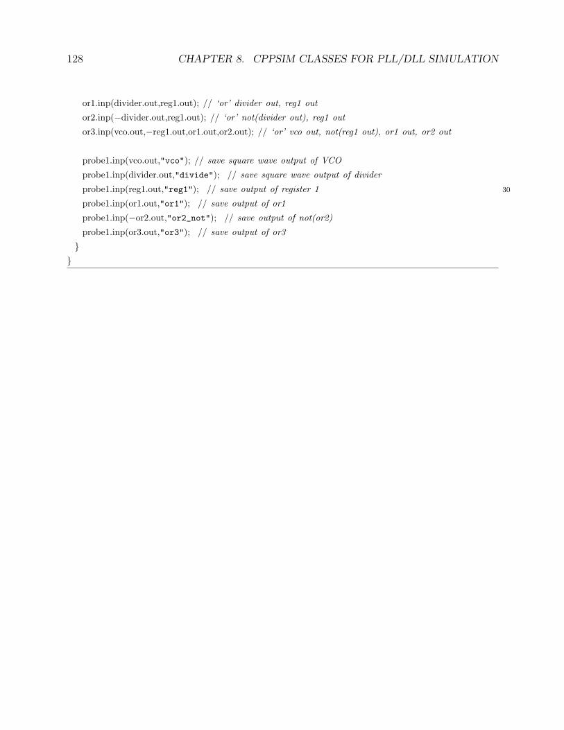
128 CHAPTER 8. CPPSIM CLASSES FOR PLL/DLL SIMULATION
or1.inp(divider.out,reg1.out); // ‘or’ divider out, reg1 out
or2.inp(−divider.out,reg1.out); // ‘or’ not(divider out), reg1 out
or3.inp(vco.out,−reg1.out,or1.out,or2.out); // ‘or’ vco out, not(reg1 out), or1 out, or2 out
probe1.inp(vco.out,"vco"); // save square wave output of VCO
probe1.inp(divider.out,"divide"); // save square wave output of divider
probe1.inp(reg1.out,"reg1"); // save output of register 1 30
probe1.inp(or1.out,"or1"); // save output of or1
probe1.inp(−or2.out,"or2_not"); // save output of not(or2)
probe1.inp(or3.out,"or3"); // save output of or3
}}

8.10. EDGEMEASURE 129
8.10 EdgeMeasure
Measures time between rising edges of its input. Normalized to a sample time equal to one.
The output is zero except at the location of edges.
Declaration
EdgeMeasure edge time1;
Variables
double out; // output is time since last edge if input is rising edge, 0 otherwise
Functions
double inp(double in); // returns out, input must be a square wave alternating between -1 and 1
Example of Usage
#include "com_blocks.h"
main()
{int i;
double Ts;
double in;
Ts = 1e−9;
Probe probe1("test.tr0",Ts); 10
Vco vco("fc + Kv*x","fc,Kv,Ts",10e6,1e6,Ts);
Divider divider;
EdgeMeasure edge time1,edge time2;
for (i = 0; i < 10000; i++)
{in = (1.0/10000.0)∗i;vco.inp(in); // frequency will gradually increase since in is a ramp
divider.inp(vco.out,10.0); // divide down VCO frequency by a factor of 10
20
probe1.inp(vco.out,"vco"); // save square wave output of VCO
probe1.inp(divider.out,"divide"); // save square wave output of divider
probe1.inp(edge time1.inp(vco.out),"vco_time");
// note: a given EdgeMeasure module cannot be used twice in one loop

130 CHAPTER 8. CPPSIM CLASSES FOR PLL/DLL SIMULATION
probe1.inp(edge time2.inp(divider.out),"divide_time");
}}
Appendix A
Example Simulation Code (Not
Auto-Generated)
This appendix provides four different examples illustrating the ability of the CppSim classes
to quickly and accurately simulate the behavior of PLL systems ranging from frequency
synthesizers to clock and data recovery circuits. These examples are NOT generated from
netlists, but rather are directly implemented in C++ code using the CppSim classes. Al-
though the netlist driven method should be used whenever possible, these examples provide
the user with a straightforward presentation of the structure and issues associated with doing
C++ simulations with the provided classes.
131
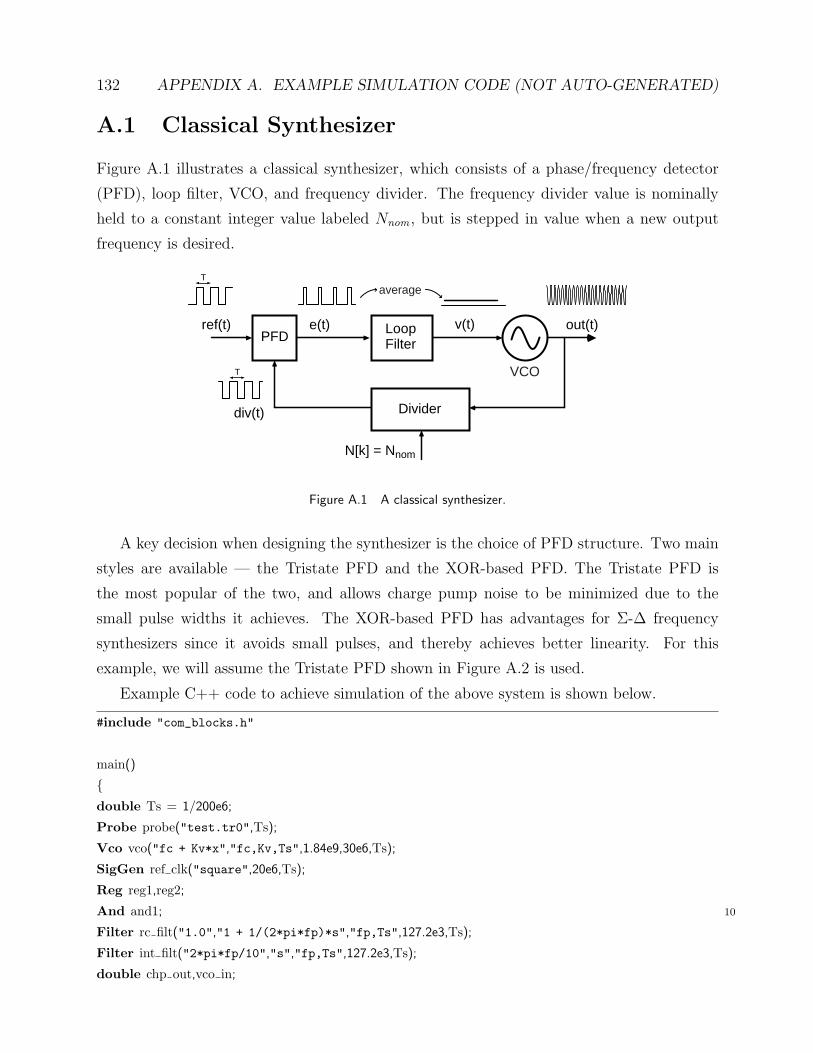
132 APPENDIX A. EXAMPLE SIMULATION CODE (NOT AUTO-GENERATED)
A.1 Classical Synthesizer
Figure A.1 illustrates a classical synthesizer, which consists of a phase/frequency detector
(PFD), loop filter, VCO, and frequency divider. The frequency divider value is nominally
held to a constant integer value labeled Nnom , but is stepped in value when a new output
frequency is desired.
PFD LoopFilter
ref(t) out(t)
Divider
T
T
e(t) v(t)
div(t)
VCO
N[k] = Nnom
average
Figure A.1 A classical synthesizer.
A key decision when designing the synthesizer is the choice of PFD structure. Two main
styles are available — the Tristate PFD and the XOR-based PFD. The Tristate PFD is
the most popular of the two, and allows charge pump noise to be minimized due to the
small pulse widths it achieves. The XOR-based PFD has advantages for Σ-Δ frequency
synthesizers since it avoids small pulses, and thereby achieves better linearity. For this
example, we will assume the Tristate PFD shown in Figure A.2 is used.
Example C++ code to achieve simulation of the above system is shown below.
#include "com_blocks.h"
main()
{double Ts = 1/200e6;
Probe probe("test.tr0",Ts);
Vco vco("fc + Kv*x","fc,Kv,Ts",1.84e9,30e6,Ts);
SigGen ref clk("square",20e6,Ts);
Reg reg1,reg2;
And and1; 10
Filter rc filt("1.0","1 + 1/(2*pi*fp)*s","fp,Ts",127.2e3,Ts);
Filter int filt("2*pi*fp/10","s","fp,Ts",127.2e3,Ts);
double chp out,vco in;

A.1. CLASSICAL SYNTHESIZER 133
D
Q
Q
D
Q
Q
R
R
ref_clk.out
vco.out
ref_clk.out
vco.out
1
1
reg1.out
reg2.out
reg1.out
reg2.out
1
-11
-1
1
-11
-1
reg1
reg2
and1
and1.out
-and1.out
Figure A.2 Tristate PFD.
int i,N;
N = 90;
for (i = 0; i < 200000; i++)
{// step desired VCO frequency by 1.0∗Kv at sample 160000
if (i == 160000) 20
N += 1;
// reference oscillator
ref clk.inp(0.0);
// PFD
reg1.inp(1.0,vco.out,−1.0,and1.out);
reg2.inp(1.0,ref clk.out,−1.0,and1.out);
and1.inp(reg1.out,reg2.out);
30
// Charge Pump
chp out = (reg2.out−reg1.out)∗.1989∗PI;
// Loop Filter
rc filt.inp(chp out);
int filt.inp(chp out);
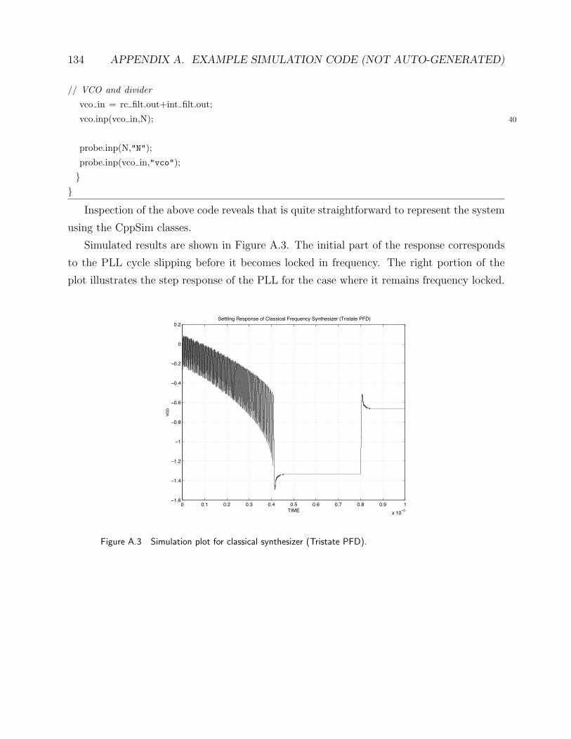
134 APPENDIX A. EXAMPLE SIMULATION CODE (NOT AUTO-GENERATED)
// VCO and divider
vco in = rc filt.out+int filt.out;
vco.inp(vco in,N); 40
probe.inp(N,"N");
probe.inp(vco in,"vco");
}}
Inspection of the above code reveals that is quite straightforward to represent the system
using the CppSim classes.
Simulated results are shown in Figure A.3. The initial part of the response corresponds
to the PLL cycle slipping before it becomes locked in frequency. The right portion of the
plot illustrates the step response of the PLL for the case where it remains frequency locked.
0 0.1 0.2 0.3 0.4 0.5 0.6 0.7 0.8 0.9 1
x 10−3
−1.6
−1.4
−1.2
−1
−0.8
−0.6
−0.4
−0.2
0
0.2
vco
TIME
Settling Response of Classical Frequency Synthesizer (Tristate PFD)
Figure A.3 Simulation plot for classical synthesizer (Tristate PFD).

A.2. Σ-Δ SYNTHESIZER 135
A.2 Σ-Δ Synthesizer
Figure A.4 illustrates a Σ-Δ frequency synthesizer. In this case, rather than remaining
constant, the divide value is dithered according to the output of a Σ-Δ modulator.
PFD ChargePump
Nsd[m]
ref(t) out(t)e(t)
div(t)
Σ−ΔModulator
v(t)
N[m]
LoopFilter
Divider
VCO
Figure A.4 A Σ-Δ frequency synthesizer.
Example C++ code to achieve simulation of the Σ-Δ synthesizer is shown below. As in
the case of the classical synthesizer, the resulting code is compact and straightforward to
implement. Simulated results are shown in Figure A.5.
#include "com_blocks.h"
main()
{double Ts = 1/200e6;
SdMbitMod sd mod("1 - 3z^-1 + 3z^-2 - 1z^-3");
Probe probe("test.tr0",Ts);
Vco vco("fc + Kv*x","fc,Kv,Ts",1.84e9,30e6,Ts);
SigGen ref clk("square",20e6,Ts);
Reg reg1,reg2; 10
And and1;
Filter rc filt("1.0","1 + 1/(2*pi*fp)*s","fp,Ts",127.2e3,Ts);
Filter int filt("2*pi*fp/10","s","fp,Ts",127.2e3,Ts);
Edge vco edge;
double chp out,vco in,in;
int i;
in = 90.3;
for (i = 0; i < 100000; i++)
{ 20

136 APPENDIX A. EXAMPLE SIMULATION CODE (NOT AUTO-GENERATED)
// step desired VCO frequency by .1∗Kv at sample 80000
if (i == 80000)
in += .1;
// SD modulator
if (vco edge.inp(vco.out))
sd mod.inp(in);
// reference oscillator
ref clk.inp(0.0);
30
// PFD
reg1.inp(1.0,vco.out,−1.0,and1.out);
reg2.inp(1.0,ref clk.out,−1.0,and1.out);
and1.inp(reg1.out,reg2.out);
// Charge Pump
chp out = (reg2.out−reg1.out)∗.1989∗PI;
// Loop Filter
rc filt.inp(chp out); 40
int filt.inp(chp out);
// VCO and divider
vco in = rc filt.out+int filt.out;
vco.inp(vco in,sd mod.out);
probe.inp(sd mod.out,"sd");
probe.inp(int filt.out,"int");
probe.inp(chp out,"chp");
probe.inp(vco in,"vco"); 50
probe.inp(reg1.out,"reg1");
probe.inp(reg2.out,"reg2");
probe.inp(vco.out,"out");
probe.inp(vco.phase,"phase");
probe.inp(ref clk.out,"ref");
}}

A.3. LINEAR CDR 137
0 0.5 1 1.5 2 2.5 3 3.5 4 4.5 5
x 10−4
−1.4
−1.2
−1
−0.8
−0.6
−0.4
−0.2
0
0.2
vco
TIME
Settling Response of �−� Frequency Synthesizer (Tristate PFD)
Figure A.5 Simulation plot for Σ-Δ synthesizer (Tristate PFD).
A.3 Linear CDR
The CppSim classes also allow straightforward simulation of clock and data recovery (CDR)
circuits. Figure A.6 illustrates a general CDR architecture that uses a phase-locked loop
to lock the phase and frequency of a VCO to that of the input data. As with frequency
synthesizers, a critical component in the design is the phase detector structure that is cho-
sen. Common choices for these detectors are the Hogge topology, which leads to linear CDR
dynamics, or the Bang-bang topology, which leads to nonlinear behavior. The Hogge topol-
ogy is often chosen for systems that have stringent requirements on the transfer function
response of the CDR to input jitter from the data sequence. The Bang-bang topology offers
superior phase acquisition speed at the expense of having nonlinear dependence on the input
jitter.
PD ChargePump
Clke(t) v(t)LoopFilter
VCO
RetimedData
Data In
Figure A.6 A PLL-based clock and data recovery circuit.

138 APPENDIX A. EXAMPLE SIMULATION CODE (NOT AUTO-GENERATED)
In this section, we will examine the simulation of a CDR that has linear dynamics by
virtue of using a Hogge phase detector. The Hogge structure is illustrated in Figure A.7.
D Q D Q
Clk
Clk
Data In
Data In
RetimedData
Retimed Data
Reg Latch
Error
Error
A
A
B
B
C
C
Figure A.7 A linear phase detector (Hogge topology).
C++ simulation code for a linear CDR system is given below. As with the synthesizer
examples, one can see that the CppSim classes allow straightforward implementation of this
system in code.
#include "com_blocks.h"
main()
{double Ts = 1/15e9;
Probe probe("test.tr0",Ts);
Vco vco("fc + Kv*x","fc,Kv,Ts",2.5e9,30e6,Ts);
SigGen prbs data("prbs",2.502e9,Ts);
Reg reg1;
Latch latch1; 10
Xor xor1,xor2;
Filter int filt("1","C*s","C,Ts",2e−9,Ts);
Filter rc filt("R","1 + 1/(2*pi*fp)*s","R,fp,Ts",1.07e3,40e6,Ts);
EdgeMeasure vco period,in period;
Rand randg("gauss");
double chp out,vco in,pd out,in;
double N dBc,f off,noise var,Kv;
int i;
/∗ VCO noise ∗/ 20
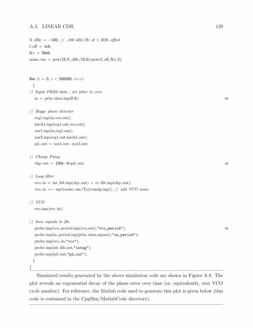
A.3. LINEAR CDR 139
N dBc = −100; // -100 dBc/Hz at 1 MHz offset
f off = 1e6;
Kv = 30e6;
noise var = pow(10,N dBc/10.0)∗pow(f off/Kv,2);
for (i = 0; i < 500000; i++)
{// Input PRBS data - set jitter to zero
in = prbs data.inp(0.0); 30
// Hogge phase detector
reg1.inp(in,vco.out);
latch1.inp(reg1.out,vco.out);
xor1.inp(in,reg1.out);
xor2.inp(reg1.out,latch1.out);
pd out = xor1.out−xor2.out;
// Charge Pump
chp out = 150e−6∗pd out; 40
// Loop filter
vco in = int filt.inp(chp out) + rc filt.inp(chp out);
vco in += sqrt(noise var/Ts)∗randg.inp(); // add VCO noise
// VCO
vco.inp(vco in);
// Save signals to file
probe.inp(vco period.inp(vco.out),"vco_period"); 50
probe.inp(in period.inp(prbs data.square),"in_period");
probe.inp(vco in,"vco");
probe.inp(int filt.out,"integ");
probe.inp(pd out,"pd_out");
}}
Simulated results generated by the above simulation code are shown in Figure A.8. The
plot reveals an exponential decay of the phase error over time (or, equivalently, over VCO
cycle number). For reference, the Matlab code used to generate this plot is given below (this
code is contained in the CppSim/MatlabCode directory).
140 APPENDIX A. EXAMPLE SIMULATION CODE (NOT AUTO-GENERATED)
x = loadsig('test.tr0');
raw period vco = evalsig(x,'vco_period');
raw period in = evalsig(x,'in_period');
%phase = extract phase(raw period vco);
[phase,avg period] = extract phase(raw period vco,raw period in);
%phase = phase-1/avg period;
phase = phase + .5; 10
% phase = phase(30000:length(phase));
plot(phase,'-k');
grid on;
xlabel('VCO rising edge number');
ylabel('Instantaneous Jitter (U.I.)');
title str = sprintf('Instantaneous Jitter of VCO in CDR: \n Steady-state RMS jitter = %5.4f mUI',1e3∗std(phasetitle(title str);
%axis([-1e3 5e4 -.2 .05])
20
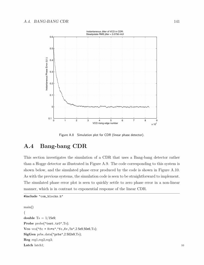
A.4. BANG-BANG CDR 141
0 1 2 3 4 5 6 7 8 9
x 104
0.1
0
0.1
0.2
0.3
0.4
0.5
0.6
VCO rising edge number
Inst
anta
neou
s P
hase
Err
or (
U.I.
)
Instantaneous Jitter of VCO in CDR: Steadystate RMS jitter = 3.0756 mUI
Figure A.8 Simulation plot for CDR (linear phase detector).
A.4 Bang-bang CDR
This section investigates the simulation of a CDR that uses a Bang-bang detector rather
than a Hogge detector as illustrated in Figure A.9. The code corresponding to this system is
shown below, and the simulated phase error produced by the code is shown in Figure A.10.
As with the previous systems, the simulation code is seen to be straightforward to implement.
The simulated phase error plot is seen to quickly settle to zero phase error in a non-linear
manner, which is in contrast to exponential response of the linear CDR.
#include "com_blocks.h"
main()
{double Ts = 1/15e9;
Probe probe("test.tr0",Ts);
Vco vco("fc + Kv*x","fc,Kv,Ts",2.5e9,50e6,Ts);
SigGen prbs data("prbs",2.502e9,Ts);
Reg reg1,reg2,reg3;
Latch latch1; 10

142 APPENDIX A. EXAMPLE SIMULATION CODE (NOT AUTO-GENERATED)
Xor xor1,xor2;
Filter int filt("2*pi*40e9","s","Ts",Ts);
EdgeMeasure vco period,in period;
Rand randg("gauss");
double chp out,vco in,pd out,in;
double N dBc,f off,noise var,Kv;
int i;
/∗ VCO noise ∗/N dBc = −90; // -90 dBc/Hz at 1 MHz offset 20
f off = 1e6;
Kv = 50e6;
noise var = pow(10,N dBc/10.0)∗pow(f off/Kv,2);
for (i = 0; i < 300000; i++)
{// Input PRBS data
in = prbs data.inp(0.0); // set jitter to zero
30
// Bang-bang phase detector
reg1.inp(in,vco.out);
reg2.inp(reg1.out,vco.out);
reg3.inp(in,−vco.out);
latch1.inp(reg3.out,−vco.out);
xor1.inp(reg1.out,latch1.out);
xor2.inp(reg2.out,latch1.out);
pd out = xor1.out−xor2.out;
// Charge Pump 40
chp out = 1e−6∗pd out;
// Loop filter
vco in = int filt.inp(chp out) + chp out∗125.0e3;vco in += sqrt(noise var/Ts)∗randg.inp(); // add VCO noise
// VCO
vco.inp(vco in);
// Save signals to file 50
probe.inp(vco period.inp(vco.out),"vco_period");

A.4. BANG-BANG CDR 143
probe.inp(in period.inp(prbs data.square),"in_period");
probe.inp(vco in,"vco");
probe.inp(int filt.out,"integ");
probe.inp(pd out,"pd_out");
}}
D Q D Q
Clk
Clk
Data In
Retimed DataReg Latch
D Q D Q
Clk Error
Data In
Retimed Data
Reg Reg
Error
A
A
BB
0
-1
1
Figure A.9 A bang-bang phase detector.

144 APPENDIX A. EXAMPLE SIMULATION CODE (NOT AUTO-GENERATED)
0 0.5 1 1.5 2 2.5 3 3.5 4 4.5 5
x 104
0.2
0.15
0.1
0.05
0
0.05
VCO rising edge number
Inst
anta
neou
s P
hase
Err
or (
U.I.
)
Instantaneous Jitter of VCO in CDR: Steadystate RMS jitter = 3.4598 mUI
Figure A.10 Simulation plot for CDR (bang-bang phase detector).

Appendix B
Hspice Toolbox for Matlab
Documentation and code written by Michael H. PerrottCopyright c© 1999 by Silicon Laboratories, Inc.
The Hspice toolbox for Matlab is a collection of Matlab routines that allow you to
manipulate and view signals generated by Hspice simulations. The primary routine is a mex
program called loadsig.mexsol that reads binary output files generated by Hspice transient,
DC, and AC sweeps into Matlab. The remaining routines are used to extract particular
signals and view them.
We will begin this document by explaining how to include the Hspice toolbox in your
Matlab session. A list of each of the current functions will then be presented. Finally, we
will provide examples of using these routines to view and postprocess signals from Hspice
output files.
B.1 Setup
To use the Hspice toolbox, simply place the included files into a directory of your choice,
and then add that directory to your Matlab path. For example, inclusion of the path
’/home/username/CppSim/HspiceToolbox’ in Matlab can be done by adding the line
addpath(’/home/username/Cppsim/HspiceToolbox’)
to the file startup.m located in your home directory. In addition, you can specify the plot
background to be black (similar to the look of Awaves) by adding another line to startup.m:
colordef none;
145

146 APPENDIX B. HSPICE TOOLBOX FOR MATLAB
Once you’ve made the above changes to startup.m, start Matlab as you normally would.
Matlab will automatically read startup.m from your home directory and execute its com-
mands.
B.2 List of Functions
The following functions are currently included in the Hspice toolbox:
• x = loadsig(’hspice_output_filename’);
– Returns a Matlab structure into variable x that includes all of the signals that
are present in the Hspice binary output file, hspice_output_filename.
• lssig(x)
– Lists all of the Hspice signal names present in the structure x.
• y = evalsig(x,’nodename’);
– Pulls out the signal nodename from the structure x and places into variable y.
The string nodename can be an expression involving several Hspice signals. If you
only performed one sweep in the simulation (as is common), then y will contain
one column. If you performed several sweeps, y will contain several columns
that correspond to the data for each sweep. If you have set the global Matlab
variable sweep to a nonzero number, however, then y will contain only one column
corresponding to the value of sweep. If sweep equals zero, all the sweep columns
are included in y.
• plotsig(x,’plot_expression’,’optional_plotspec’)
– Plots signals from the structure x according to the expression given in plot_expression.
The string optional_plotspec is used to create logscale plots; it can be specified
as logx, logy, or logxy. The string plot_expression specifies the nodenames,
and corresponding mathematical operations, that you would like to view. In this
expression, commas delimit curves to be overlayed and semicolons delimit sepa-
rate subplots on the same figure. All numeric node names should be prepended
by ‘@’ to distinguish them from constants. Some examples of using plotsig are:
B.3. EXAMPLES 147
∗ plotsig(x,’v1,v2;v3’): overlays v1 and v2 on the same subplot, and plots
v3 on a separate subplot.
∗ plotsig(x,’(v1+v2)^2; log(abs(v3))’): plots the listed expressions on
separate subplots.
∗ plotsig(x,’db(v1); ph(v1)’,’logx’): plots the magnitude (in dB) and
phase (in degrees) of v1 on a semilogx axis.
∗ plotsig(x,’v1+@2+3’): plots the addition of node v1, node 2, and the con-
stant 3.
∗ plotsig(x,’integ(TIME,v1); avg(TIME,v2)’): plots the integral of v1
and average of v2 on separate subplots.
• xlima
– Sets the x-limits of all subplots in a figure. Three options are possible:
∗ xlima: sets all subplots to the same x-axis as the last subplot that was zoomed
into,
∗ xlima([xs xe]): sets all subplots to the x-axis limits specified,
∗ xlima(’auto’): resets all subplots back to autoscaling.
– Note: ylima and xylima functions are also provided. See comments in ylima.m
and xylima.m for proper usage.
• eyesig(x,period,start_off,’nodename’)
– Creates an eye diagram for nodename contained in x with the specified period.
All data samples prior to start_off are ignored when creating the diagram (useful
for removing the influence of transient effects from the eye diagram). The string
nodename can be an expression involving several variables.
B.3 Examples
Viewing Signals
Use the Matlab command cd to go to a directory containing a binary transient, DC, or AC
sweep file generated from Hspice. We will assume a filename of test.tr0, and now list a
series of Matlab commands that will be used to display nodes q and qb in that file.
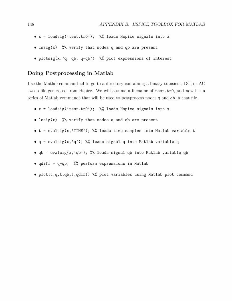
148 APPENDIX B. HSPICE TOOLBOX FOR MATLAB
• x = loadsig(’test.tr0’); %% loads Hspice signals into x
• lssig(x) %% verify that nodes q and qb are present
• plotsig(x,’q; qb; q-qb’) %% plot expressions of interest
Doing Postprocessing in Matlab
Use the Matlab command cd to go to a directory containing a binary transient, DC, or AC
sweep file generated from Hspice. We will assume a filename of test.tr0, and now list a
series of Matlab commands that will be used to postprocess nodes q and qb in that file.
• x = loadsig(’test.tr0’); %% loads Hspice signals into x
• lssig(x) %% verify that nodes q and qb are present
• t = evalsig(x,’TIME’); %% loads time samples into Matlab variable t
• q = evalsig(x,’q’); %% loads signal q into Matlab variable q
• qb = evalsig(x,’qb’); %% loads signal qb into Matlab variable qb
• qdiff = q-qb; %% perform expressions in Matlab
• plot(t,q,t,qb,t,qdiff) %% plot variables using Matlab plot command