88
i CPT-based Axial Static Capacity Approaches to Evaluate Pile Driveability in Sand Putri Suciaty Gandina

i
CPT-based Axial Static Capacity
Approaches to Evaluate Pile
Driveability in Sand
Putri Suciaty Gandina

ii
iii
CPT-based Axial Static Capacity
Approaches to Evaluate Pile Driveability
in Sand
By
Putri Suciaty Gandina
in partial fulfilment of the requirements for the degree of
Master of Science
in Civil Engineering
at the Delft University of Technology.
to be defended publicly on Friday 10th of August 2018 at 10:00 AM.
Thesis committee
Prof. Dr. Kenneth G. Gavin, TU Delft
Dr. Luke J. Prendergast, TU Delft
Dr. Federico Pisano, TU Delft
Dr. Bas van Dijk, Fugro
Dr. Phil Vardon, TU Delft
An electronic version of this thesis is available at http://repository.tudelft.nl/.

iv

v
Preface
This thesis is final task in fulfilment of the requirement for master’s degree in Civil Engineering with
specialisation in Geo-Engineering at Delft University of Technology (TU-Delft). I would like to use this
opportunity to acknowledge some people for their contribution in this thesis.
First of all, praise be to Allah SWT, Most Gracious, so that I can finish my study.
I would like to thank my supervisor and former chairman, Prof. Kenneth G. Gavin. Big thanks for the
opportunity to do a thesis related with pile foundation. Thank you for all of his advice, technical support
and guidance during my thesis phases.
Many thanks for my daily supervisor Dr.Luke J.Prendergast. He has been there every moment when I
need advice. Luke kept me calm when I was too worried about doing something wrong in the analysis.
He patiently checked my work and gives me feedback during writing thesis report. Thank you for always
being nice, without his guidance this thesis would not be achieved.
Dr.Federico Pisano as my chairman. I would like to thank you for his commitment. Thanks for
immediately respond my e-mail and give a feedback during the meeting. Thank you for his support
during my timeline deadline, without his support I would not finish my study on time.
Dr.Bas van Dijk as my committee members. I would like to thank you for his commitment and dedication
to come to the meeting despite his busy schedule. Thanks for immediately respond my e-mail and give
technical suggestion during the meeting.
Dr.Phil Vardon as my committee member. Thank you for his commitment to join my committee member.
I cannot finish my study on time without his support during public defence.
Thank you to my family for their endless support throughout my entire phases in my life. My mother
who always pray for me. My sister, who always patiently listening to my random story. I would like to
thank Rafil Fikriyan for his love and kindly support. Thanks to all my friends who always be there through
up and down in my thesis weird mood. They always provide me with comfort. Lastly, I would like to
thank LPDP scholarship which gives me financial support during my study in the Netherlands.
Putri Suciaty Gandina
Delft, August 2018

vi

vii
Abstract The demand for offshore wind farm installation is increasing in recent years as the concern in
using sustainable energy source is rising. One of the primary steps in constructing offshore
wind farm is the pile installation which is a high-risk activity due to the expensive offshore
installation vessels requirement. Any factor which can result in delaying the pile installation
process will lead to financial losses. Therefore, a comprehensive driveability analysis using
an efficient pile model is favourable. From the driveability model, the suitable pile equipment
can be selected consider the underlying soil condition. The selected equipment must be
capable of installing pile into the target depth without overstressing the pile within the design
time.
An essential component in driveability model is to estimate the static resistance to driving
(SRD). The SRD in analogues with axial static pile capacity approaches. These approaches
use the Cone Penetration Test (CPT) data to determine the axial pile capacity. Factors such
as the friction fatigue effect, stress equalisation and soil plugging are related and affect axial
pile capacity. These factors are integrated into driveability analysis in this study to provide a
more reliable result when using CPT-based approaches to calculate static axial capacity.
Pile installation data records from Blessington, Ireland are used as a part of the axial static
load test programme. Pile load tests have been performed on open-ended steel piles with a
diameter of 0.34m. The site condition consists of glacial deposit dense sand. From this
database, the performance of driveability models by using the available and modified CPT-
based approaches (e.g., the UWA-05, ICP-05, and Fugro-05) are assessed in this study. The
modified model considers the friction fatigue effect, the pile ageing effect, the soil plugging
condition, the pile tip mobilisation and the base residual stresses while the SRD is calculated
by using the available CPT-based approaches.
The recent CPT-based axial static capacity methods are investigated to see if they can be
used as a reliable method to determine static resistance to driving (SRD) profiles. The SRD
profiles are comparable to the axial static capacity approach which account for the pile ageing
effect, the soil tip displacement, and residual stresses during driving. The pile ageing effect
that is incorporated in the model as installation resistance is set for the time equals to zero,
unlike with the static capacity load test which is derived after a certain time after end
installation. The total resistance that is recorded for open-ended small diameter piles is
calculated to model the pile tip mobilisation which is associated with the base resistance. The
residual base stresses are modelled for each hammer blow during driving. The wave equation
analysis uses a combination of the SRD profiles and dynamic soil components, pile properties
and installation equipment resulting in total resistance as the blow count prediction.
This study provides information on how to model driveability analysis from the recent CPT-
based axial static capacity approaches. The models one modified to include related factors
that affected pile installation process. The performance of predicted blow counts result from
unmodified and modified CPT-based methods are appraised and compared to the recorded
blow count as a model verification. The UWA-05 modified model can be considered as an
appropriate model to estimate pile driveability from CPT-based axial static capacity approach.

viii

ix
Contents
Abstract ............................................................................................................................. vii
List of Figures .................................................................................................................... xi
List of Tables .................................................................................................................... xiii
List of Symbols and Abbreviations ................................................................................ xiv
1 Introduction ...................................................................................................................... 1
1.1 Research Question ...................................................................................................... 2
1.2 Approach to Research ................................................................................................. 2
1.3 Limitations ................................................................................................................... 3
2 Pile Driveability ................................................................................................................ 4
2.1 Installation of piles into the soil .................................................................................... 5
2.2 Static Resistance to Driving ......................................................................................... 7
2.3 The Dynamic Approach ............................................................................................... 8
2.4 The CPT-based Static Capacity Methods .................................................................... 9
2.4.1 Shaft Friction ....................................................................................................... 10
2.4.2 Base Resistance ................................................................................................. 12
3 Modelling Process ......................................................................................................... 16
3.1 Database Assessment ............................................................................................... 17
3.2 Time Effect ................................................................................................................ 20
3.3 Base Resistance-Displacement ................................................................................. 21
3.4 Residual Base Effect ................................................................................................. 22
4 Analysis & Results ......................................................................................................... 25
4.1 Base Resistance-Displacement Curve ....................................................................... 25
4.2 Static Capacity Approach Comparison ...................................................................... 27
4.3 Residual Base Modification ....................................................................................... 29
5 Parameter Study ............................................................................................................ 32
5.1. Damping ................................................................................................................... 33
5.2. Quake ....................................................................................................................... 33
5.3. Stroke Height ............................................................................................................ 34
5.4. Hammer Efficiency ................................................................................................... 35
6 Case Study – Rotterdam Harbour ................................................................................. 36
6.1. Database at Rotterdam ............................................................................................. 36
6.2. Static capacity in clay ............................................................................................... 38
6.3. Blow Count Prediction .............................................................................................. 39
x
7 Conclusions and Recommendation.............................................................................. 45
Bibliography ...................................................................................................................... 48
A Shaft Friction SRD ..................................................................................................... 51
B Blessington site Result ............................................................................................. 55
B.1 Base Resistance-Displacement ................................................................................. 55
B.2 Blow Count Comparison ............................................................................................ 58
B.3 Residual Base Stresses ............................................................................................ 62
C Rotterdam site Result ................................................................................................ 67
C.1 Base Resistance-Displacement ................................................................................ 67
C.2 Blow Count Comparison ........................................................................................... 68
C.3 Residual Base Stresses ............................................................................................ 71
xi
List of Figures
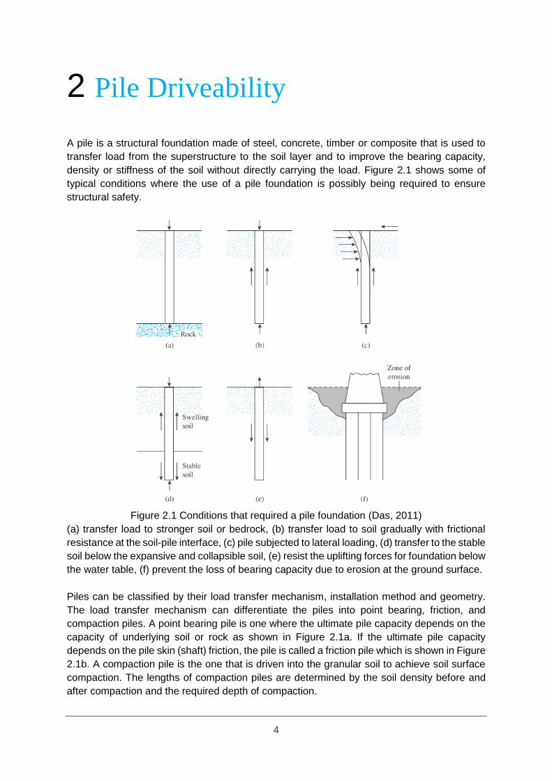
Figure 2.1 Conditions that required a pile foundation (Das, 2011) ......................................... 4
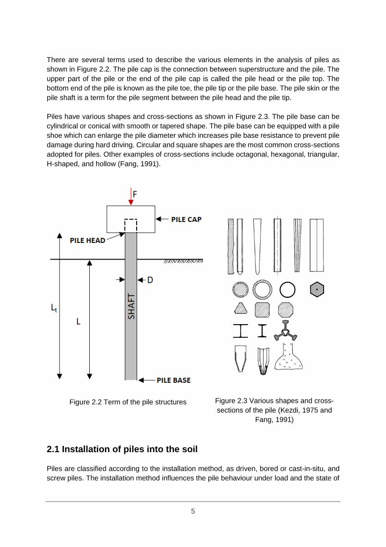
Figure 2.2 Term of the pile structures .................................................................................... 5
Figure 2.3 Various shapes and cross-sections of the pile (Kezdi, 1975 and Fang, 1991) ...... 5
Figure 2.4 Type of pile driving hammers (modified after Das, 2011) ...................................... 6
Figure 2.5 The quake definition (Byrne et al., 2018) .............................................................. 9
Figure 2.6 Possible sources of friction fatigue (Jardine and Chow, 2007) ........................... 11
Figure 2.7 Kinematics of friction fatigue close to the pile tip
(modified after White and Bolton, 2004; Kirwan, 2014) ........................................ 11
Figure 2.8 Soil flow and profiles of radial stress (White and Bolton, 2005) .......................... 14
Figure 3.1 Flow chart driveability analysis ........................................................................... 16
Figure 3.2 Soil properties at Blessington ............................................................................. 18
Figure 3.3 Measurement during driving ............................................................................... 20
Figure 3.4 Base resistance-settlement model (Gavin and Lehane, 2007)............................ 21
Figure 3.5 The development of residual base stress during pile driving .............................. 23
Figure 4.1 Base resistance-displacement curves at various depth ...................................... 26
Figure 4.2 Recorded and predicted blow counts comparison with CPT-based axial static
capacity approach ............................................................................................. 28
Figure 4.3 UWA unit base resistance with varying residual base stresses added ................ 30
Figure 4.4 Recorded and predicted blow count with residual base stresses added ............. 31
Figure 5.1 Parameters analysis compare to the UWA-05 method ....................................... 32
Figure 5.2 Effect of damping ............................................................................................... 33
Figure 5.3 Effect of quake ................................................................................................... 34
Figure 5.4 Effect of (a) stroke height (b) hammer efficiency ................................................ 35
Figure 6.1 Soil database at Rotterdam ................................................................................ 37
Figure 6.2 The correlation of α values developed from the load test
(after Doherty and Gavin, 2011) ........................................................................ 38
Figure 6.3 Base resistance-displacement curves at various driving depth ........................... 41
Figure 6.4 Predicted blow counts comparison using CPT-based approaches at pile P1 ...... 42
Figure 6.5 The UWA modified model with residual base stresses added analysis results ... 43
Figure A.1 The friction fatigue effect in the shaft friction SRD at Blessington ...................... 53
Figure A.2 The friction fatigue effect in the shaft friction SRD at Rotterdam ........................ 54
Figure B.1 Base resistance-displacement curves at various depth in Blessington site ........ 58
Figure B.2 Recorded and predicted blow count comparison at Blessington site .................. 62
Figure B.3 Recorded and modified additional base residual stresses at Blessington........... 63
Figure B.4 The UWA unit base resistance with varying residual base stresses added at
Blessington site ................................................................................................. 65
Figure B.5 Recorded and predicted blow count with residual base stresses added at
Blessington site ................................................................................................. 66
xii
Figure C.1 Base resistance-displacement curves at various driving depth in
Rotterdam site .................................................................................................. 68
Figure C.2 Recorded and predicted blow count comparison at Rotterdam .......................... 70
Figure C.3 The UWA unit base resistance with varying residual base stresses added at
Rotterdam site .................................................................................................. 72
Figure C.4 Recorded and predicted blow count with residual base stresses added at
Rotterdam site .................................................................................................. 73

xiii
List of Tables
Table 2.1 The CPT-based design method for shaft friction calculation of driven piles in
sand (modified after Xu, 2007) ............................................................................ 13
Table 2.2 The CPT-based design method for unit base resistance calculation of driven
piles in sand (modified after Xu, 2007) ................................................................ 15
Table 3.1 Hammer properties at Blessington ...................................................................... 19
Table 6.1 CPT-based design method calculation of driven piles in clay .............................. 40
Table B.1 The base resistance – displacement average along the pile at Blessington ........ 55
Table B.2 The CoV from the average blow count along the pile depth at Blessington ......... 59
Table C.1 The base resistance – displacement average at 30-35m pile depth
in Rotterdam ....................................................................................................... 67
Table C.2 The CoV from the average blow count at 30-35m at Rotterdam .......................... 69
xiv
List of Symbols and Abbreviations
𝑎 Parameter in ICP-05 Method for incorporate open-ended piles in tension
𝐴𝑏 Base area
𝐴𝑟 Area ratio
𝐴𝑟,𝑒𝑓𝑓 Effective Area Ratio
𝑏 Parameter in ICP-05 Method for incorporate compression or tension load tests
𝐷 External pile diameter
𝐷50 Soil particle diameter at which 50% of the mass of soil sample is smaller
𝐷𝑖 Internal pile diameter
𝐷𝑟 Relative density of the soil
𝑒 Void ratio
𝐸𝑏𝑒𝑞 Young’s modulus
𝐸𝑜 Small strain elastic stiffness of the soil
𝐹𝑡𝑖𝑚𝑒 Time factor for shaft friction calculation
𝐺𝑜 Shear modulus of the soil
ℎ Distance above pile tip level
∆ℎ𝑝𝑙𝑢𝑔 Change in plugging length
𝐿 Pile penetration length below ground level
∆𝐿𝑝𝑖𝑙𝑒 Change in pile penetration length
𝑃𝑟𝑒𝑓 Reference atmospheric stress
𝑞𝑎𝑛𝑛 Unit bare resistance at pile annulus
𝑞𝑏 Unit base resistance
𝑞𝑏0.1 Unit base resistance when 0.1 pile diameter mobilise
𝑞𝑏,𝑛%(𝑧) Additional step wise unit base resistance at z
𝑞𝑏,𝑟𝑒𝑠 Base residual stresses
𝑞𝑐 Cone tip resistance
𝑞𝑐,𝑎𝑣𝑔 Average cone tip resistance
𝑞𝑛 Net cone resistance
𝑞𝑡 Total cone resistance
𝑄𝑏 Axial base resistance
𝑄𝑠 Axial shaft resistance
∑𝑄𝑠,𝐿
Cumulative shaft resistance at the pile tip depth
∑𝑄𝑠,𝐿−1
Cumulative shaft resistance at the previous depth increment
𝑄𝑡 Total axial capacity
𝑅 Pile outer radius
𝑅𝑖 Inner pile radius
𝑅∗ Equivalent pile radius
𝑡 Time after driving
𝑡𝑤 Pile wall thickness
𝑇 Time
𝑢𝑜 Pore-water pressure
𝑉𝑠 Shear wave velocity
∆𝑦 Radial displacement of interface zone during dilation
𝑧 Element depth

xv
𝛼 Adhesion factor
𝛿𝑓 Constant volume interface friction angle
𝜋 Pi, mathematical constant = 0.314
𝜎′3 Effective confining stress (triaxial test)
𝜎𝑣𝑜 Total vertical overburden pressure
𝜎′𝑟𝑐 Radial effective stress after installation and stress equalisation
𝜎′𝑟𝑓 Radial effective stress at failure
𝛥𝜎′𝑟𝑑 Increase in radial stress due to dilation at the soil-structure interface during
loading
𝜏𝑓 Shaft friction at failure
𝜏𝑓,𝑖𝑛 Internal shaft friction
𝜏𝑓,𝑛𝑒𝑔 Negative shaft friction
∆𝜏𝑓,𝑎𝑣𝑔 Average shaft friction
𝜈 Poisson’s ratio
API American Petroleum Institute
bgl Below ground level
CoV Coefficient of Variation
CPT Cone Penetration Test
FFR Final Filling Ratio
GRLWEAP GRL’s Wave Equation Analysis of Pile Driving
IAC Intact Ageing Curve
ICP Imperial College Pile
IFR Incremental Filling Ratio
NGI Norwegian Geotechnical Institute
SRD Static Resistance to Driving
UWA University of Western Australia
1
1 Introduction
Pile driving is a high-risk activity, especially in the offshore environment. Inefficient driveability
can cause delay and material damage that may lead to financial overspending. Selected
equipment must be capable of installing the pile at the target depth within the given time-frame
without overstressing the pile. Therefore, a comprehensive driveability analysis is essential to
any offshore project. Driveability must consider all aspects, such as soil condition and soil-
structure interaction, driving equipment performance and pile specifications such as the
geometry and material properties.
Any driveability study requires calculation of Static Resistance to Driving (SRD). SRD is
analogous to the axial capacity of a pile and represents the cumulative increase in shaft
capacity associated with further pile penetration and encompasses a base resistance that is
associated with each driving increment. The SRD is a measure of the expected resistant of
the pile to driving and develops during pile installation. Schneider and Harmon (2010) claim
that SRD is similar to pile static axial capacity except for the resistance often differs due to
consolidation, stress equalisations, and ageing (capacity increases over time).
The total resistance of a pile driving is commonly presented in terms of the blow count required
to drive the pile or as resistance curves. Typically, the number of blows that it takes the
hammer to drive the pile to a certain depth (per 0.25m usually) and the soil resistance at the
time of driving are measures used to appraise the difficulty associated with a given pile driving.
A combination of SRD and associated dynamic components is the input required to conduct
a total resistance of a pile driving. Wave equation analysis is essential to incorporate the
dynamic component increase due to inertia and the viscous rate effects. The obligatory inputs
for wave equation analysis are the SRD, the dynamic components that are represented by
damping and a quake values, the pile and the hammer properties. Analysis of this solve the
wave equation that simulates the responses of a pile from each hammer blow.
Cone Penetration Test (CPT) is commonly used in construction projects in Europe where
almost every project has a minimum of one single complete CPT. There are various CPT-
based methods to determine the axial static capacity of piles. These load capacity calculation
methods are derived from pile load tests that are usually conducted between 10 and 30 days
after pile driving. Past studies have indicated that static pile capacity may increase over time
after pile driving (Jardine et al., 2006; Gavin et al., 2013; Karlsrud et al., 2014; Kirwan, 2014;
Gavin et al., 2015). That study suggests that pile resistance during installation will be lower
than the available model calculation. A time factor should be applied to determine the
driveability from the available CPT-based static axial capacity methods.
During pile driving, shear resistance reduction occurs as the distance from the pile to the tip
increases. This phenomenon is known as friction fatigue. Schneider and Harmon (2010)
suggest calculating the pseudo average shaft friction to accommodate changes in the shape
of shear resistance distribution during pile driving.

2
The pile penetration per blow during driving is less than the failure criteria of base capacity
from the ICP-05, Fugro-05 and UWA-05 model which suggests a pile tip displacement of 0.1
of the pile diameter. A reduction factor is required to consider the actual pile tip displacement
during driving. On the other hand, the residual load on the pile base may have been
significantly miss-represented which could lead to considerable error in UWA base resistance
method (Xu, 2007). Ignoring residual loads can lead to an underestimating of the base
resistance in a compression load test which can cause significant errors when correlating base
resistance with cone resistance (White and Bolton, 2005). This residual stress study suggests
stress may be higher at the pile toe. Therefore, taking an additional residual base will be
reasonable to develop a proper model.
The purpose of this research thesis is to develop an efficient model for driveability analysis
using CPT-based axial static capacity methods. Moreover, several parameters will be
examined to determine which factors influence pile driveability. For this purpose, the analysis
will use Blessington database (see Section 3.1). The Blessington project consists of 7 steel
open-ended full-scale test pile at Blessington, Ireland. The pile penetration length is 7m with
a diameter of 0.34m. The soil profile at this location form of a very dense, fine sand deposit.
The groundwater located at 13m below the ground level.
1.1 Research Question
The objective of the research is to gain knowledge on the performance of CPT-based axial
static capacity approaches to evaluate pile driveability in the sand. Therefore, the research
question can be listed into work as follows:
1. How to calculate axial static capacity using available CPT-based methods?
2. How to develop an efficient model for the driveability analysis using the CPT-based axial
capacity methods?
3. What parameters primarily affect pile driveability analysis?
1.2 Approach to Research To be able to answer above mention research question, this thesis will consist of several
phases:
1. A literature review that consists available method to conduct driveability analysis. Several
CPT-based methods commonly used for the axial static capacity analysis in sand such
as the UWA-05, ICP-05, and Fugro-05.
2. Collecting data available from site location to perform driveability analysis. Required data
consist of soil data, pile properties and hammer properties. Soil data will be needed to
calculation soil model using the available CPT-based method. Perform driveability data
will depend upon wave equation analysis which requires all these data. Wave equation
analysis will be implemented by using driveability analysis software, GRLWEAP.
3. Modifying model to determine an efficient driveability model that will be validated with
the actual blow counts data. To be able to make an efficient prediction, modification

3
needed with considering several parameters in driveability analysis. The result of
modified method will be validated by comparison with recorded blow counts in the field.
4. Sensitivity analysis varying the primary parameters of driveability analysis. It is essential
to perform sensitivity analysis to quantify the change in the primary parameters affecting
driveability analysis results.
5. The application of driveability model will be applied in pile driven in different soil
conditions. The CPT-based axial static capacity in clay layers is also assessed. Later,
this model will be validated with recorded blow count data which is available from the
site.
1.3 Limitations
There are several limitations that confine all result and conclusion in this study:
1. Methods chosen are only the CPT-based approaches for axial static capacity
calculation.
2. The driving stresses and installation time is disregarded in this study.
3. Organic soil that presents in the soil profile will be recognised as clay layer.
4. An external environmental condition such as wave at the offshore pile will be ignored.
5. The weight of the driving system (all components between the hammer and pile top) are
excluded in performing wave equation analysis.
4
2 Pile Driveability
A pile is a structural foundation made of steel, concrete, timber or composite that is used to
transfer load from the superstructure to the soil layer and to improve the bearing capacity,
density or stiffness of the soil without directly carrying the load. Figure 2.1 shows some of
typical conditions where the use of a pile foundation is possibly being required to ensure
structural safety.
Figure 2.1 Conditions that required a pile foundation (Das, 2011)
(a) transfer load to stronger soil or bedrock, (b) transfer load to soil gradually with frictional
resistance at the soil-pile interface, (c) pile subjected to lateral loading, (d) transfer to the stable
soil below the expansive and collapsible soil, (e) resist the uplifting forces for foundation below
the water table, (f) prevent the loss of bearing capacity due to erosion at the ground surface.
Piles can be classified by their load transfer mechanism, installation method and geometry.
The load transfer mechanism can differentiate the piles into point bearing, friction, and
compaction piles. A point bearing pile is one where the ultimate pile capacity depends on the
capacity of underlying soil or rock as shown in Figure 2.1a. If the ultimate pile capacity
depends on the pile skin (shaft) friction, the pile is called a friction pile which is shown in Figure
2.1b. A compaction pile is the one that is driven into the granular soil to achieve soil surface
compaction. The lengths of compaction piles are determined by the soil density before and
after compaction and the required depth of compaction.
5
There are several terms used to describe the various elements in the analysis of piles as
shown in Figure 2.2. The pile cap is the connection between superstructure and the pile. The
upper part of the pile or the end of the pile cap is called the pile head or the pile top. The
bottom end of the pile is known as the pile toe, the pile tip or the pile base. The pile skin or the
pile shaft is a term for the pile segment between the pile head and the pile tip.
Piles have various shapes and cross-sections as shown in Figure 2.3. The pile base can be
cylindrical or conical with smooth or tapered shape. The pile base can be equipped with a pile
shoe which can enlarge the pile diameter which increases pile base resistance to prevent pile
damage during hard driving. Circular and square shapes are the most common cross-sections
adopted for piles. Other examples of cross-sections include octagonal, hexagonal, triangular,
H-shaped, and hollow (Fang, 1991).
Figure 2.2 Term of the pile structures
Figure 2.3 Various shapes and cross-
sections of the pile (Kezdi, 1975 and
Fang, 1991)
2.1 Installation of piles into the soil
Piles are classified according to the installation method, as driven, bored or cast-in-situ, and
screw piles. The installation method influences the pile behaviour under load and the state of

6
stress in the surrounding soil (Poulos and Davis, 1984). Pile driving process causes soil
rearrangement, in loose sand driving will advantages rather than pile boring due to increase
in relative density.
Based on the nature of the soil placement during pile installation, the piles can be divided into
displacement piles and non-displacement piles. Displacement piles are those whereby the
installation process causes soil densification that leads to stress changes in the soil. Driven
piles or jacking piles are an example of displacement piles. Bored piles which give very little
change in the state of stress in the surrounding soil are called non-displacement piles.
Piles are driven into the ground using hammers. Pile driving hammer can be classified as
diesel hammer or internal combustion hammer, external combustion hammer, and vibratory
hammer as shown in Figure 2.4. According to working principles, the external combustion
hammers are classified as steam hammer, air hammer, hydraulic hammer, and drop hammer.
Drop hammer as shown in Figure 2.4a which the oldest type of hammer is lifted with hoist and
rope and allow to drop from a certain height. Drop hammer has a slow rate of blows hence
hydraulic hammer developed with adjustable ram fall height and various energy settings
during the downstroke. Vibratory hammer as shown in Figure 2.4b consists of pairs counter-
rotating weights (oscillator) that cancel the presence of horizontal forces resultant and
generate centrifugal force. A clamp is used to transfer centrifugal force from oscillator into
vertical forces which drive the pile.
The diesel hammer as shown in Figure 2.4c consists of the ram, anvil block, and fuel-injection
system. The ram is released with gravity and fuel is squirt at the top of the anvil. The ram
drops compress the air-fuel mixture which causes the heated air combusts after a short delay.
This combustion process is delayed due to the time required for fuel mix with the heated air
to ignite. The combustion pushes the pile downward into the soil and raises the ram. The ram
will ascends to a certain stroke height and begin a new cycle. Almost all hammers impact the
pile head, but certain external combustion hammers can be driven at the pile tip or in the pile
shaft (Pile Dynamics Inc., 2010a).
(a) Drop hammer (b) Vibratory hammer (c) Diesel hammer
Figure 2.4 Type of pile driving hammers (modified after Das, 2011)

7
During the pile driving process, a pile cap is attached to the pile head, and a pile cushion may
be used in between the pile head and the pile cap. The hammer drops on the hammer cushion
that is placed on the pile cap. The cushion function is to reduce the impact-force and distribute
the force.
2.2 Static Resistance to Driving
Soil resistance during driving is a combination of static and dynamic components. The static
resistance to driving (SRD) is a static component of the soil resistance during driving which is
analogues with static axial capacity. The SRD has shaft friction which changes with each
driving increment. Unlike static capacity that only has single base resistance, the SRD profile
has base resistance for each driving increment. The difference between the static capacity
and the SRD is due to time effect or ageing, consolidation, stress equalisation, and definition
of soil failure in static load tests (Schneider and Harmon, 2010).
The same as the axial static capacity, plugging condition of the pile tip during each driving
increment which represents by IFR will affect base resistance in the SRD. In fully coring
condition (IFR=1), the unit end bearing is occurred on the pile annulus (qann), and the pile shaft
friction is occurred both internal (𝜏𝑓,𝑖𝑛) and external (𝜏𝑓) along the shaft surface area. Alm and
Hamre (2001) and Schneider and Harmon (2010) suggest to reduce unit friction to 50% and
apply on both inside and outside of the pile wall which is the same as applying full external
shaft friction without internal shaft friction. The static axial capacity calculation is addressed
further in Section 2.4.
The shaft resistance distribution associated with each pile penetration is altered due to the
friction fatigue effect. The axial static capacity method (i.e. UWA-05, ICP-05, and Fugro-05) is
difficult for estimating the change in shaft friction distribution during pile driving. Therefore, an
appropriate technique is introduced to account for the change of the shaft friction distribution.
The parameters influence prediction bearing graph and blow counts from SRD which have a
maximum to minimum effect are a fraction of resistance from Qb and Qs, pile penetration depth,
and shape of shaft friction distribution (Alm and Hamre, 2001). The shape of the shaft friction
has a minimum effect, so Schneider and Harmon (2010) suggest to calculate the pseudo
average shaft friction (∆𝜏𝑓,𝑎𝑣𝑔) using change in shaft capacity between two successive depth
increment follows :
∆𝜏𝑓,𝑎𝑣𝑔 =∑ 𝑄𝑆,𝐿−∑ 𝑄𝑆,𝐿−1
𝜋𝐷 ∆𝐿 Equation 2.1
Where ∑QS,L is the cumulative shaft resistance at the pile tip depth, ∑QS,L-1 is the cumulative
shaft resistance at the previous depth increment, ΔL is the depth increment, D is the pile
diameter. Friction fatigue cause ∆𝜏𝑓,𝑎𝑣𝑔 is less than 𝜏𝑓 near the pile tip and possible to have
negative value due to decreasing soil strength profile in the soil and small values of ΔL. The
detail explanation about friction fatigue is addressed in Section 2.4.1.

8
2.3 The Dynamic Approach
The dynamics components that increase soil resistance during driving are due to inertial and
viscous rate effects. Soil dynamics components are accounted in wave equation analysis use
GRLWEAP program by Pile Dynamics Inc. (2010b). This program will solves the one-
dimensional wave equation theory as proposed by Smith (1960) based on mass discretisation
with pile-soil interaction simplification as
𝜕𝑢2
𝜕𝑡2= 𝑐2 𝜕𝑢2
𝜕𝑥2 Equation 2.2
Where c is a velocity of propagation of longitudinal strain wave along the rod (hammer, driving
system and pile) = √𝐸/𝜌 , x is a direction of the longitudinal axis of the pile, u is a displacement
of pile cross section in the x direction, t is time, E is the elastic modulus and ρ is the mass
density.
GRL’s Wave Equation Analysis of Pile Driving (GRLWEAP) is a computer program which
simulates motions and forces along the pile when driven by hammer (Pile Dynamics Inc.,
2010a). The program predicts the blow counts from SRD inputs and soil dynamics
components by varying hammer and pile properties. Hammer type, hammer stroke height,
hammer efficiency, driving systems such as cushion and helmet are hammer properties inputs
that needed to do wave equation analysis. Furthermore, wave equation analysis also can give
analysis output as installation stresses along the pile and driving time to install the pile.
Soil damping and quake are soil dynamic components to incorporate inertia and viscous
effect. Lowery et al. (1968) conduct a triaxial test in sand and shows that damping value varied
from 0.16 to 0.65 s/m and increase as effective confining stress (σ’3) and sand density
increases (void ratio e decreases). The soil damping depends on soil type and independent
of the total soil resistance and pile size properties. Smith (1960) recommend taking toe
damping larger than shaft or skin damping. Smith shaft and base damping of 0.25 and 0.5 s/m
respectively use for the UWA-05 method in sandy soil (Schneider and Harmon, 2010). The
other calculation method (ICP-05 and Fugro-05) will use a GRLWEAP recommendation for
shaft and base damping of 0.16 and 0.5 s/m in sandy soil.
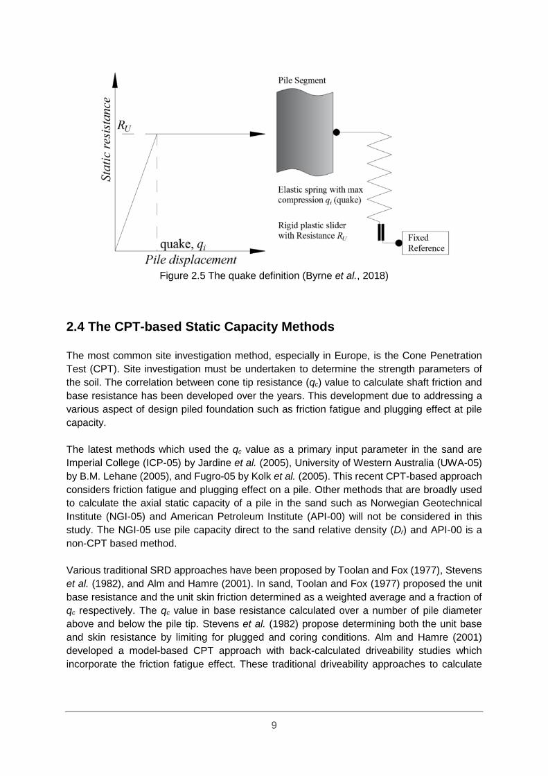
The load-deformation relationship during pile driving is defined by a static resistance and a
quake value for each spring shown in Figure 2.5. The quake value represents a maximum
elastic pile displacement before yield. The journal that is written by Lowery et al. (1968) state
difficulty in determining the quake value for the various type of soil condition. In the absence
of the quake value, it is recommended to use 2.5mm for both shaft and base quake value.
9
Figure 2.5 The quake definition (Byrne et al., 2018)
2.4 The CPT-based Static Capacity Methods
The most common site investigation method, especially in Europe, is the Cone Penetration
Test (CPT). Site investigation must be undertaken to determine the strength parameters of
the soil. The correlation between cone tip resistance (qc) value to calculate shaft friction and
base resistance has been developed over the years. This development due to addressing a
various aspect of design piled foundation such as friction fatigue and plugging effect at pile
capacity.
The latest methods which used the qc value as a primary input parameter in the sand are
Imperial College (ICP-05) by Jardine et al. (2005), University of Western Australia (UWA-05)
by B.M. Lehane (2005), and Fugro-05 by Kolk et al. (2005). This recent CPT-based approach
considers friction fatigue and plugging effect on a pile. Other methods that are broadly used
to calculate the axial static capacity of a pile in the sand such as Norwegian Geotechnical
Institute (NGI-05) and American Petroleum Institute (API-00) will not be considered in this
study. The NGI-05 use pile capacity direct to the sand relative density (Dr) and API-00 is a
non-CPT based method.
Various traditional SRD approaches have been proposed by Toolan and Fox (1977), Stevens
et al. (1982), and Alm and Hamre (2001). In sand, Toolan and Fox (1977) proposed the unit
base resistance and the unit skin friction determined as a weighted average and a fraction of
qc respectively. The qc value in base resistance calculated over a number of pile diameter
above and below the pile tip. Stevens et al. (1982) propose determining both the unit base
and skin resistance by limiting for plugged and coring conditions. Alm and Hamre (2001)
developed a model-based CPT approach with back-calculated driveability studies which
incorporate the friction fatigue effect. These traditional driveability approaches to calculate

10
SRD will not assess future in this study, as the development of this method more reliable for
the pile with a large diameter.
The ultimate capacity is the summation of the shaft and base resistance as written in the
following
𝑄𝑡 = 𝑄𝑠 + 𝑄𝑏 = 𝑃 ∫ 𝜏𝑓 𝑑𝑧 + 𝐴𝑏 𝑞𝑏 Equation 2.3
Where: Qs is the total shaft capacity, Qb is the total base capacity, P is a perimeter of the pile
(P=πD for a circular pile and P= 4B for square pile), 𝜏𝑓 is the local shaft friction at failure along
the shaft of a pile, z is the embedded shaft length, Ab is a base area (𝐴𝑏 = 𝜋𝐷2
4 for a circular
pile, and 𝐴𝑏 = 𝐵2 for square pile), qb is the base resistance assumes a displacement of 0.1D
as failure criteria (at a pile head for ICP-05, at a pile tip for UWA-05 and Fugro-05), and D is
the pile outer diameter.
2.4.1 Shaft Friction
The shaft friction develops following a Coulomb failure criterion as proposed by Jardine et al.
(2005) and Lehane et al. (2005) as shown below
𝜏𝑓 = 𝜎′𝑟𝑓 𝑡𝑎𝑛 𝛿𝑓 = (𝜎′
𝑟𝑐 + 𝛥𝜎′𝑟𝑑) 𝑡𝑎𝑛 𝛿𝑓 Equation 2.4
Where 𝜎′𝑟𝑓 is a radial effective stress at failure, 𝛿𝑓 is a constant volume interface friction
angle, 𝜎′𝑟𝑐 is a radial effective stress after installation and equalisation, and 𝛥𝜎′
𝑟𝑑 is a change
in radial stress due to dilation at the soil-structure interface during loading.
The increase in radial stress due to loading stress path relates to lateral expansion or dilation
(𝛥𝜎′𝑟𝑑) at the soil-structure interface during loading can be modelled using the cavity
expansion theory (Lehane, 1992). The change in radial stress is a function of soil shear
stiffness normalised by the pile diameter and radial expansion which is influenced by a pile
shaft roughness (∆y). Pile shaft roughness depends on the material in the shear zone. The
roughness of concrete piles is higher than steel piles (0.01-0.02mm). The dilation or shear
zone thickness is approximately ten times the mean size of the soil (D50). In a full-scale pile
test which has a D/D50 between 1000-8000, the magnitude of 𝛥𝜎′𝑟𝑑 is negligible. However, in
a laboratory test with D/D50 less than 1000, 𝛥𝜎′𝑟𝑑 will have a significant contribution (Lehane,
1992). Morphology or particle shape affects 𝛥𝜎′𝑟𝑑, an angular particle has greater dilation
than a more rounded particle (Santamarina and Cho, 2004).
The radial effective stress after installation and equalisation (𝜎′𝑟𝑐) is a function of cone
resistance and relates to the friction fatigue effect. The friction fatigue phenomenon refers to
the behaviour of soil shear resistance reduction as a vertical distance from the pile tip to a
specific soil horizon increases. This phenomenon leads to high stress close to the pile tip and
contraction of the shear zone along the pile shaft with each installation cycle (Kirwan, 2014).
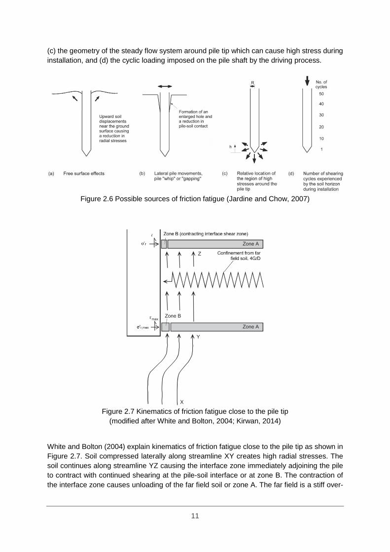
Chow (1996) listed the possible cause reduction in radial effective stress as shown in Figure
2.6 as (a) the free surface effect which can affect up to 20D in clay and less in sand, (b) the
lateral movement during driving can cause whip or gapping until 4D below the soil surface,
11
(c) the geometry of the steady flow system around pile tip which can cause high stress during
installation, and (d) the cyclic loading imposed on the pile shaft by the driving process.
Figure 2.6 Possible sources of friction fatigue (Jardine and Chow, 2007)
Figure 2.7 Kinematics of friction fatigue close to the pile tip
(modified after White and Bolton, 2004; Kirwan, 2014)
White and Bolton (2004) explain kinematics of friction fatigue close to the pile tip as shown in
Figure 2.7. Soil compressed laterally along streamline XY creates high radial stresses. The
soil continues along streamline YZ causing the interface zone immediately adjoining the pile
to contract with continued shearing at the pile-soil interface or at zone B. The contraction of
the interface zone causes unloading of the far field soil or zone A. The far field is a stiff over-

12
consolidated soil due to pile installation. As a stiff soil unloading response, a small contraction
of the interface zone causes significant radial stress reduction applied by the far field on the
pile shaft. As the relative depth to pile tip (h) increases, the interface zone contracts and the
spring unloads, thus reducing the shaft friction on the pile.
The friction fatigue effect is represented in ICP-05, and Fugro-05 method by the relative depth
to pile tip (h) normalised by an equivalent radius of the pile (R*). Gavin and Lehane (2007)
state that the local shaft friction was affected by the degree of plugging during installation as
defined by Incremental Filling Ratio (IFR). White and Bolton (2005) show that profiles of radial
stress along the pile shaft can be differentiated by an effective area ratio (Ar,eff) which is a
measure of the soil displacement during installation determined by the IFR. Xu (2007) state to
avoid term h/R*, the shaft friction UWA-05 method uses h/D and Ar,eff to incorporate friction
fatigue and soil displacement in the specific soil horizon during pile installation. Summaries
shaft friction calculation method in sand shows in Table 2.1.
2.4.2 Base Resistance
The ultimate base stress is defined as the unit base resistance developed at a pile
displacement equating to 10% of the pile diameter (qb0.1). The base resistance calculation is
a function of average cone resistance (qc,avg) which depends on the method of pile installation,
the surface scale effect, and the pile end conditions (closed and open-ended). The degree of
soil displacement during installation has a significant effect on pile response to static loading
(Gavin and Lehane, 2007). The base resistance stress for an unplugged open-ended pile acts
in the annular area, whereas the plugged pile will have bearing capacity in the full area of the
pile.
During pile driving, the soil plug condition inside the pile affects the behaviour of dynamic
driving resistance and static bearing capacity. White and Bolton (2005) illustrated the
schematics streamline of soil flow and profiles of radial stress in closed-ended piles, fully
coring or unplugged open-ended piles and partially plugged open-ended piles as shown in
Figure 2.8. In the fully plugged condition, soil displaces roughly equal to the solid pile volume
which causes an increase in the radial and base stress thus resulting in higher driving
resistance and static capacity (Xu, 2007). In an unplugged condition which usually occurs for
a large diameter pile, the soil displacement is approximately the same as the pile volume
causing lower radial and base stress.
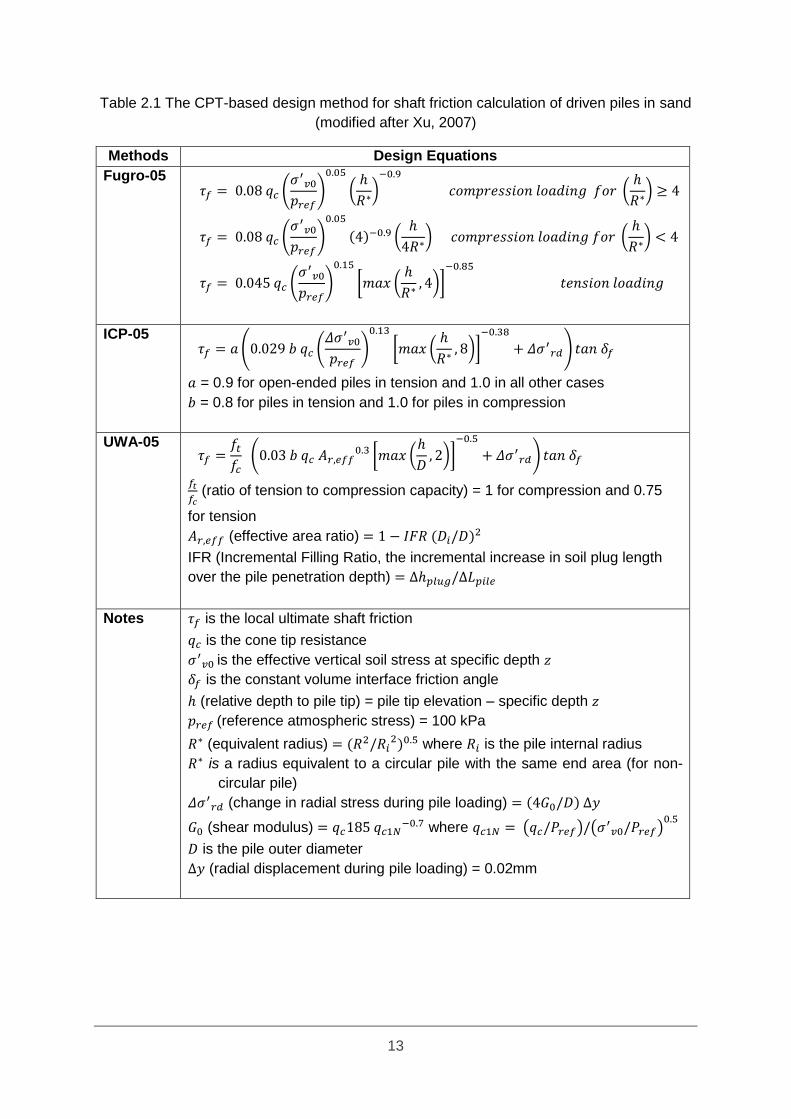
13
Table 2.1 The CPT-based design method for shaft friction calculation of driven piles in sand
(modified after Xu, 2007)
Methods Design Equations
Fugro-05 𝜏𝑓 = 0.08 𝑞𝑐 (
𝜎′𝑣0
𝑝𝑟𝑒𝑓)
0.05
(ℎ
𝑅∗)
−0.9
𝑐𝑜𝑚𝑝𝑟𝑒𝑠𝑠𝑖𝑜𝑛 𝑙𝑜𝑎𝑑𝑖𝑛𝑔 𝑓𝑜𝑟 (ℎ
𝑅∗) ≥ 4
𝜏𝑓 = 0.08 𝑞𝑐 (𝜎′
𝑣0
𝑝𝑟𝑒𝑓)
0.05
(4)−0.9 (ℎ
4𝑅∗) 𝑐𝑜𝑚𝑝𝑟𝑒𝑠𝑠𝑖𝑜𝑛 𝑙𝑜𝑎𝑑𝑖𝑛𝑔 𝑓𝑜𝑟 (
ℎ
𝑅∗) < 4
𝜏𝑓 = 0.045 𝑞𝑐 (𝜎′
𝑣0
𝑝𝑟𝑒𝑓)
0.15
[𝑚𝑎𝑥 (ℎ
𝑅∗, 4)]
−0.85
𝑡𝑒𝑛𝑠𝑖𝑜𝑛 𝑙𝑜𝑎𝑑𝑖𝑛𝑔
ICP-05 𝜏𝑓 = 𝑎 (0.029 𝑏 𝑞𝑐 (
𝛥𝜎′𝑣0
𝑝𝑟𝑒𝑓)
0.13
[𝑚𝑎𝑥 (ℎ
𝑅∗, 8)]
−0.38
+ 𝛥𝜎′𝑟𝑑) 𝑡𝑎𝑛 𝛿𝑓
𝑎 = 0.9 for open-ended piles in tension and 1.0 in all other cases
𝑏 = 0.8 for piles in tension and 1.0 for piles in compression
UWA-05 𝜏𝑓 =
𝑓𝑡
𝑓𝑐 (0.03 𝑏 𝑞𝑐 𝐴𝑟,𝑒𝑓𝑓
0.3 [𝑚𝑎𝑥 (ℎ
𝐷, 2)]
−0.5
+ 𝛥𝜎′𝑟𝑑) 𝑡𝑎𝑛 𝛿𝑓
𝑓𝑡
𝑓𝑐 (ratio of tension to compression capacity) = 1 for compression and 0.75
for tension
𝐴𝑟,𝑒𝑓𝑓 (effective area ratio) = 1 − 𝐼𝐹𝑅 (𝐷𝑖/𝐷)2
IFR (Incremental Filling Ratio, the incremental increase in soil plug length
over the pile penetration depth) = ∆ℎ𝑝𝑙𝑢𝑔/∆𝐿𝑝𝑖𝑙𝑒
Notes 𝜏𝑓 is the local ultimate shaft friction
𝑞𝑐 is the cone tip resistance
𝜎′𝑣0
is the effective vertical soil stress at specific depth 𝑧
𝛿𝑓 is the constant volume interface friction angle
ℎ (relative depth to pile tip) = pile tip elevation – specific depth 𝑧
𝑝𝑟𝑒𝑓 (reference atmospheric stress) = 100 kPa
𝑅∗ (equivalent radius) = (𝑅2/𝑅𝑖2)0.5 where 𝑅𝑖 is the pile internal radius
𝑅∗ is a radius equivalent to a circular pile with the same end area (for non-
circular pile)
𝛥𝜎′𝑟𝑑 (change in radial stress during pile loading) = (4𝐺0/𝐷) ∆𝑦
𝐺0 (shear modulus) = 𝑞𝑐185 𝑞𝑐1𝑁−0.7 where 𝑞𝑐1𝑁 = (𝑞𝑐/𝑃𝑟𝑒𝑓)/(𝜎′
𝑣0/𝑃𝑟𝑒𝑓)0.5
𝐷 is the pile outer diameter
∆𝑦 (radial displacement during pile loading) = 0.02mm

14
Figure 2.8 Soil flow and profiles of radial stress; δr is radial displacement of soil element at
pile wall (White and Bolton, 2005)
The Incremental Filling Ratio (IFR=∆ℎ𝑝𝑙𝑢𝑔/∆𝐿𝑝𝑖𝑙𝑒) is zero when there is no soil plug movement
inside the pile, between zero and one when the pile is partially plugged and one when the pile
is fully coring. The base condition when installing a large diameter of an open-ended pile in
the uniform soil is likely fully coring or unplugged (IFR=1). The soil will tend to be plugged or
move along with the pile increment (0<IFR<1) under slow loading condition such as a static
load test.
The UWA-05 approach that is proposed by Lehane, Schneider and Xu (2005) including the
effect of partial plugging during installation on base resistance mobilised at the base
displacement of 10% of the pile diameter. The UWA-05 takes the final filling ratio (FFR) as
IFR at the final stage of installation to calculate base resistance. The other methods such as
ICP-05 and Fugro-05 neglect partially-plugging condition in base resistance calculation. The
Fugro-05 also calculate base resistance at pile tip displacement of 10% diameter of the pile
whereas ICP-05 takes pile head displacement for 10% of the pile diameter. Both Fugro-05
and ICP-05 will take base resistance as fully coring or fully plugged. The CPT-based
calculation methods to compute unit base resistance in sand are summarised in Table 2.2.
During pile installation process, the driving force will push the pile until exceeding the ultimate
pile capacity resulting pile move forward into the ground. When removing driving force at the
pile top (zero pile load) the base resistance (Qb) will equal with downward shaft resistance
(Qs,neg), and the pile tends to move backwards or rebound. At zero pile loading, unit base
residual and downward skin friction refers as a base residual stresses (qb,res) and negative
skin friction (𝜏𝑓,𝑛𝑒𝑔) respectively.

15
Table 2.2 The CPT-based design method for unit base resistance calculation of driven piles
in sand (modified after Xu, 2007)
Methods Base
Condition Design Equation
Sa
nd
Fugro-05
Close &
open 𝑞𝑏0.1
𝑞𝑐,𝑎𝑣𝑔= 8.5 (
𝑃𝑟𝑒𝑓
𝑞𝑐,𝑎𝑣𝑔)
0.5
𝐴𝑟0.25
ICP-05
Close 𝑞𝑏0.1
𝑞𝑐,𝑎𝑣𝑔= 𝑚𝑎𝑥𝑖𝑚𝑢𝑚 [1 − 0.5 𝑙𝑜𝑔 (
𝐷
𝐷𝐶𝑃𝑇) , 0.3]
Open If 𝐷𝑖 ≥ 2.0 (𝐷𝑟 − 0.3) or 𝐷𝑖 ≥ 0.083 𝑞𝑐,𝑎𝑣𝑔
𝑃𝑟𝑒𝑓 𝐷𝐶𝑃𝑇
pile is unplugged 𝑞𝑏0.1
𝑞𝑐,𝑎𝑣𝑔= 𝐴𝑟
if not, pile is plugged
𝑞𝑏0.1
𝑞𝑐,𝑎𝑣𝑔= 𝑚𝑎𝑥𝑖𝑚𝑢𝑚 [0.5 − 0.25 𝑙𝑜𝑔 (
𝐷
𝐷𝐶𝑃𝑇) , 0.15 , 𝐴𝑟]
Non-
circular
𝑞𝑏0.1
𝑞𝑐,𝑎𝑣𝑔= 0.7
UWA-05
Close &
open
𝑞𝑏0.1
𝑞𝑐,𝑎𝑣𝑔= 0.15 + 0.45 𝐴𝑟,𝑒𝑓𝑓
Notes 𝐷 is the pile outer diameter
𝐷𝑖 is the pile inner diameter
𝐷𝐶𝑃𝑇 (conus diameter) = 0.036 m
𝐴𝑟 (area ratio) = 1 − (𝐷𝑖/𝐷)2
𝐴𝑟,𝑒𝑓𝑓 (effective area ratio) = 1 − 𝐹𝐹𝑅 (𝐷𝑖/𝐷)2
FFR (final filling ratio) = IFR (= ∆ℎ𝑝𝑙𝑢𝑔/∆𝐿𝑝𝑖𝑙𝑒) average over
the last 3𝐷𝑖 of the pile penetration
𝑞𝑐,𝑎𝑣𝑔 = 𝑞𝑐 average ±1.5𝐷 over pile tip level for Fugro-05
and ICP-05
𝑞𝑐,𝑎𝑣𝑔 = 𝑞𝑐 average using the Dutch averaging technique
for the UWA-05*)
Dr (nominal relative density) = 0.4 𝑙𝑛 [(𝑞𝑐,𝑡𝑖𝑝/22)/(𝑃𝑟𝑒𝑓/
𝜎′𝑣0)
0.5]
*) 𝑞𝑐,𝑎𝑣𝑔 = 𝑞𝑐 average ± ±1.5𝐷 for UWA-05 as SRD input

16
3 Modelling Process
This chapter discusses all aspects to consider when developing driveability analysis models.
These aspects are the time effect, soil displacement during driving and base residual loads
after each driving increment. Furthermore, this chapter presents the inputs data from
Blessington site which are required to perform driveability analysis such as soil parameters,
hammer specification, and pile properties including material and geometry. This chapter also
presents recorded blow counts and measured incremental filling ratio (IFR). These data are
essential to verify blow count predictions from this study.
Figure 3.1 shows a flow chart of driveability analysis in this study. The soil data and pile
properties will be needed to calculate shaft and base resistance with axial static capacity
methods (i.e., UWA-05, ICP-05 and Fugro-05). The calculated base resistance is inputted
directly to the SRD profile, while the shaft resistance must be calculated with the pseudo
average skin friction before inputted in the SRD profile. The wave equation analysis is
performed with a combination of soil data in the form of the SRD and dynamics soil component
(i.e., quake and damping), pile, and hammer properties. The total resistance (blow counts) is
resulted from the wave equation analysis. The first modification into the model integrates the
base resistance-displacement to the base resistance and add the time factor to the shaft
resistance. More modification is applied by including the base residual stresses to the base
resistance in the SRD profile.
Figure 3.1 Flow chart driveability analysis

17
3.1 Database Assessment
The project consists of 7 steel open-ended full-scale test piles at Blessington, southwest of
Dublin, Ireland. Soil properties and ground conditions at the Blessington site have been used
in the various experiments as reported in Gavin and Lehane (2007), Gavin et al. (2013),
Prendergast et al. (2013), and Kirwan (2014). The soil profile at this site consists of very dense
sand in the heavily over-consolidated state due to glacial deposit history and previous
significant overburden pressure. The groundwater table is approximately 13m below ground
level (bgl). The in-situ water content relatively uniform at 10-12% above the water table.
Blessington pile tests are conducted above the water table where pore pressure dissipates
almost immediately. This test does not compromise the comparability of the site to offshore
deposits where the soil is fully saturated as pile capacities are determined by effective stresses
(Gavin et al., 2013).
The sand relative density ranges between 90% and 100%. The particle size (D50) was varied
between 0.1mm and 0.15mm based on particle size distribution analysis from samples located
between 0.7-2m bgl. From the grain size analysis, the soil is well-graded angular sand with 5-
10% fines content (percentage of clay or silt particle). The sand has a unit weight of 20 kN/m3.
The constant volume friction angle from ring shear test, the triaxial test is 36˚ and 37˚. Particle
morphology (particle size, angularity and roundness) have been correlated to the constant
volume friction angle. Kirwan (2014) link particle morphology (particle size, angularity and
roundness) at Blessington site with the constant volume friction angle give results of 30˚ and
32˚.
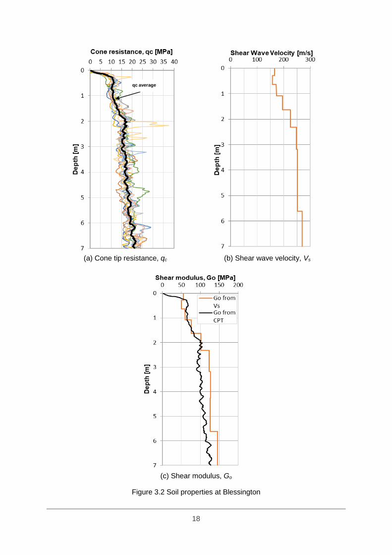
A total of 10 CPTs was conducted at the site. Cone tip resistance (qc) profile shows at Figure
3.2a indicate that qc ranging from 10 MPa at 2m bgl to 20 MPa at 7m bgl. The shear wave
velocity (Vs) shows at Figure 3.2b obtained in the field using the multi-channel analysis of
surface wave (MASW) method. The soil shear modulus (Go) profiles are derived from Vs are
shown in Figure 3.2c. This Go profiles has a comparable ratio with Go/qc of 6 as suggested in
Prendergast et al. (2013) which is applicable for unknown Vs value. The assumption of
Poisson’s ratio (ν) equal to 0.1 is used at very small strain levels. The peak friction correlated
with the CPT qc value and based triaxial test give similar result range from 54˚ near ground
surface to 42˚ at 7m bgl.
At Blessington site, seven open-ended piles named S1-S7 were driven into the ground. The
total pile length of 8.76m were driven up to 7m bgl except for pile S7 which driven until 6.5m
bgl. All piles are steel piles with Young’s modulus value of 2x10¹¹ N/m2 and have identical
geometry with an external diameter (D) of 0.34m, internal diameter (Di) of 0.312m, and wall
thickness (tw) of 0.014m. Blessington pile tests can be considered as a representative of
typical offshore piles geometries with the diameter to wall thickness D/tw ratio of 24.3 and
length to diameter L/D ratio S1-S6 and S7 of 20.6 and 19.1, respectively (Kirwan, 2014).
Offshore piles have D/tw ratio between 15 and 45 (Jardine and Chow, 2007), and a diameter
between 0.66m and 2.13m which are paired with pile penetration between 26m and 87m bgl
(Overy and Sayer, 2007).
18
(a) Cone tip resistance, qc (b) Shear wave velocity, Vs
(c) Shear modulus, Go
Figure 3.2 Soil properties at Blessington
qc average

19
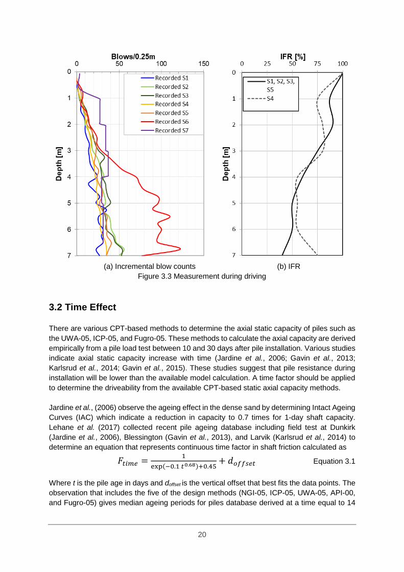
Blow count records at Blessington for all piles are plotted in Figure 3.3a. All piles tend to
increase in blow counts with depth. Blow count recorded shows that pile S4 has low blow
counts compared to S2, S3 and S5. Pile S6 gives highest blow count result compare to the
other piles. The blow counts recorded are not directly comparable since the piles had different
hammers and stroke heights except for piles S2-S5. Table 3.1 shows hammer properties at
Blessington pile tests. Pile S1-S5 and S6-S7 were driven using 4000kg Junttan PM16 and
5000kg Junttan PM20 respectively as a piling hammer. Piles S1 and pile S2-S5 were driven
with the same constant stroke height of 0.4m and 0.3m accordingly. Pile S6 had combine
stroke height from 0.2m for the first four meter and 0.35m for the rest installation. Pile S7 had
stroke height varies along the pine penetration, begin with 0.2m until 0.3m in 0.025m
increment stroke height.
Table 3.1 Hammer properties at Blessington
Pile
Name
Penetration
length [m] Hammer Cushion Stroke height [m]
S1 7 4000kg Junttan PM16 None 0.4
S2 7 4000kg Junttan PM16 None 0.3
S3 7 4000kg Junttan PM16 None 0.3
S4 7 4000kg Junttan PM16 None 0.3
S5 7 4000kg Junttan PM16 None 0.3
S6 7 5000kg Junttan PM20 50mm ash timber 0.2 (0-4m) &
0.35 (4-7m)
S7 6.5 5000kg Junttan PM20 50mm ash timber 0.2 - 0.3m
(increment 0.025m)
Figure 3.3b shows Incremental Filling Ratio (IFR) measure during pile installation. All piles
developed a similar IFR profile. Pile S1, S2, S3 and S5 were nearly fully coring or unplugged
(IFR=1) over the first meter of the pile penetration and becoming partially plugged (IFR=0.4)
at the end of driving with 2.45m final plug depth. Pile S4 has less plugging during installation
indicate with IFR profile with IFR=0.75 at the end of driving with 2.26m final plug depth. IFR
measurement from S6 is not considered as reliable due to significant scatter at 2m final
penetration with 2.56m final plug depth. Pile S7 experience more plugging which is indicated
by deeper final plug depth (3.3m) and lower IFR at the end of driving. The calculation of pile
capacity UWA method requires IFR that will be taken from S1, S2, S3, S5 as representative
IFR value.
Pile S6 has the highest blow counts despite there being no significant difference in cone tip
resistance (qc) value near this pile location compared to the other piles. This condition could
be resulted because pile S6 has lower stroke height for the first 2m than the other piles even
though It has higher hammer energy. Another possibility is due to pile S6 has a slightly higher
final plug depth which gives higher resistance as a consequence pile driving becomes more
difficult. As noted from Kirwan (2014) pile S6 was driven 1-year after S1-S5, the distance
between S6 pile is 6.4D which larger than 6D as the minimum recommendation distance to
avoid pile group effect noted in Yang (2006).
20
(a) Incremental blow counts (b) IFR
Figure 3.3 Measurement during driving
3.2 Time Effect
There are various CPT-based methods to determine the axial static capacity of piles such as
the UWA-05, ICP-05, and Fugro-05. These methods to calculate the axial capacity are derived
empirically from a pile load test between 10 and 30 days after pile installation. Various studies
indicate axial static capacity increase with time (Jardine et al., 2006; Gavin et al., 2013;
Karlsrud et al., 2014; Gavin et al., 2015). These studies suggest that pile resistance during
installation will be lower than the available model calculation. A time factor should be applied
to determine the driveability from the available CPT-based static axial capacity methods.
Jardine et al., (2006) observe the ageing effect in the dense sand by determining Intact Ageing
Curves (IAC) which indicate a reduction in capacity to 0.7 times for 1-day shaft capacity.
Lehane et al. (2017) collected recent pile ageing database including field test at Dunkirk
(Jardine et al., 2006), Blessington (Gavin et al., 2013), and Larvik (Karlsrud et al., 2014) to
determine an equation that represents continuous time factor in shaft friction calculated as
𝐹𝑡𝑖𝑚𝑒 =1
exp(−0.1 𝑡0.68)+0.45+ 𝑑𝑜𝑓𝑓𝑠𝑒𝑡 Equation 3.1
Where t is the pile age in days and doffset is the vertical offset that best fits the data points. The
observation that includes the five of the design methods (NGI-05, ICP-05, UWA-05, API-00,
and Fugro-05) gives median ageing periods for piles database derived at a time equal to 14

21
days and doffset equal to zero. This time factor can be applied to define shaft friction during
driving with a time equal to zero. Based on this calculation, the time factor of 0.69 is applied
for shaft friction SRD calculation.
Time effect results from the changes in the total stress and pore pressure due to soil
displacement during the pile driving (Schneider and Harmon, 2010). The pile ageing
observation at Blessington is controlled by a combination of creep and interface roughness.
Creep leads to an increase in the radial effective stress equalisation and enhanced dilation
while the increase in the interface roughness actuates large mobilised pile capacities (Gavin
et al., 2013).
3.3 Base Resistance-Displacement
Laboratory and field test indicated the degree of soil displacement during driving affect the pile
response during static loading (Paik et al., 2003). The unit base resistance definition proposed
by the CPT-based axial capacity methods such as UWA-05, ICP-05, and Fugro-05 are
assumed pile displacement of 0.1D (outer pile diameter). During pile installation, pile
experiences less displacement than 0.1D. Besides that, fully coring pile or unplugged pile
(IFR=1) will experience less displacement than close-ended piles. As mentioned in Section
2.4.2, the UWA-05 method is the only method that considers partially plugging condition which
is represented by the Final Filling Ratio (FFR) value. This means that there is a possibility for
integrating actual displacement with the UWA-05 method to produce base resistance model
that resemble actual driving process.
Figure 3.4 Base resistance-settlement model (Gavin and Lehane, 2007)

22
Byrne et al. (2018) propose the implementation of the three-stage base resistance-
displacement model (Gavin and Lehane, 2007) to estimate the base resistance mobilise
during each hammer impact. Figure 3.4 shows the idealised base resistance-displacement
model that is consisted of the unit base resistance (qb) versus the pile tip displacement (wb)
normalised by pile diameter (D). The ratio of wb/D is calculated for every depth from the actual
blow counts that is recorded. The base stiffness formulation at the three-stage qb – wb
relationship based on (Gavin and Lehane, 2007). In the first stage, no pile tip movement
occurs until the residual base stresses (qb,res) is exceeded.
In the second stage, the relationship between qb and wb/D is linear until the strain level (wby)
of 0.015D (Byrne et al., 2018). The strain level is controlled by stress history at the pile base.
The magnitude of strain level depends on equivalent Young’s modulus (Ebeq) which
comparable with a very small strain elastic stiffness (Eo) at the in-situ stress level. The
expression for the shear modulus (Go) correlation with the Eo and the linear stage of the curve
are represented by following
𝐸0 = 2𝐺𝑜(1 + 𝜈) Equation 3.2
𝑞𝑏 = [𝑘1 (𝑤𝑏
𝐷)] + 𝑞𝑏,𝑟𝑒𝑠 Equation 3.3
𝑘1 = (4
𝜋) [
𝐸0
1−𝑣2] Equation 3.4
Where Eo is a small strain elastic stiffness, Go is the shear modulus, ν is the Poisson’s ratio,
wb is the pile tip displacement, D is the outer pile diameter, and qb,res is the residual base
resistance.
The last stage, the non-linear part where wby/D < wb/D < 0.10 is approximately parabolic, but
in this research, it will be simplified by another linear part. In this stage, the level of prestress
that occurs in the sand at the pile tip causes the significant strain degradation in base
resistance increase. The maximum base resistance from UWA occurs when displacement
0.1D.
𝑞𝑏 = 𝑘2 [(𝑤𝑏
𝐷) − 0.015] + 0.015𝑘1 Equation 3.5
𝑘2 =𝑦2− 𝑦1
𝑥2− 𝑥1=
𝑞𝑏01,𝑈𝑊𝐴− 0.015 𝑘1
0.085 Equation 3.6
Where wb is the tip displacement, D is the outer pile diameter, (x1 ; y1) = (0.015 ; 0.015 k1), (x2
; y2) = (0.1 ; qb01,UWA), and qb01,UWA is the unit base resistance from UWA-05 method.
3.4 Residual Base Effect
During driving, the pile will experience compression due to the hammer blow and tension due
to zero pile loading. The hammer blow results in the driving force will push the pile forward
into the ground. At zero pile loading, tension force occurs at the pile will tend to move

23
backwards or rebound. In this condition, the residual base stress (qb,res) at the pile base area
will equate with negative skin friction (𝜏𝑓,𝑛𝑒𝑔) along the pile shaft. Figure 3.5 illustrate the
development of residual base stress during the pile driving.
Paik et al. (2003) state that the presence of residual base stresses did not affect the ultimate
bearing capacity during the axial static load test due to the summation of residual shaft and
base for the pile will equal to zero. However, the qb,res must be acknowledged when considering
the pile driveability analysis due to the proportion of base and shaft resistance. Except in
ultimate bearing capacity calculation, ignoring residual load will overestimate the shaft
resistance and underestimate the base resistance.
(a) Pile in compression (b) Residual stresses at zero pile loading
Figure 3.5 The development of residual base stress during pile driving
Alawneh and Husein Malkawi (2000) propose a method to estimate the post-driving base
residual stresses as a function of the pile penetration length, pile diameter, pile area, shear
modulus and pile Young’s modulus. This method gives residual stresses that range between
0 and 4000 kPa which represent the stiff-short pile in the loose sand and the flexible-long pile
in the dense sand, respectively. Paik et al. (2003) measure the residual stress at Pigeon River
site with 0.356m diameter closed and open-ended piles that give a similar result between 11-
14% of qc.
The estimation of the residual base stress method is highly empirical. Pile with the same
installation method in a similar soil condition will have a similar residual load. There is no
method which is reliable to estimate the magnitude of the residual base stresses without future
F
τf(z) τf,neg(z)
F = 0
qb(z) qb,res(z)
(a) (b)
24
adjustment based on site soil condition. This research will assess the sensitivity analysis
incorporate the residual base stresses (qb,res) for every UWA-05 unit base resistance. The
residual base stress is range between 1% and 10% of the qc value as recommend in Byrne et
al. (2018).
The base resistance assessment estimates the residual base stress that incorporates the time
effect and degree of the pile tip displacement. Firstly, the sensitivity analysis of an additional
unit base resistance at every penetration depth is calculated as follows.
𝑞𝑏,𝑛%(𝑧) = {1 ; 2 ; 5 ; 8 ; 10} % 𝑞𝑐 Equation 3.7
Where qc is the cone tip resistance, 𝑛 is an additional number, and 𝑧 is the element depth.
The second and third steps are essential to convert stresses to load due to equilibrium occurs
when the negative shaft resistance (Qs,neg) equals to the base resistance (Qb). The second
step is the calculation of the base resistance from additional stepwise the unit base resistance
along the pile base area.
𝑄𝑏,𝑛%(𝑧) = 𝑞𝑏,𝑛%(𝑧) 𝐴𝑏 Equation 3.8
Where 𝑞𝑏,𝑛%(𝑧) is an additional 𝑛% of unit base resistance at depth-𝑧, and 𝐴𝑏 is the pile base
area. Thirdly, the negative shaft resistance calculation at every pile depth following skin friction
UWA-05 method (𝜏𝑓,𝑈𝑊𝐴(𝑧)) for the pile in tension are incorporated with the time effect.
𝑄𝑠,𝑛𝑒𝑔(𝑧) = 0.75 𝐹𝑡𝑖𝑚𝑒 𝜏𝑓,𝑈𝑊𝐴(𝑧) 𝐴𝑠(𝑧) Equation 3.9
Where 𝐹𝑡𝑖𝑚𝑒 is a time factor, 𝜏𝑓,𝑈𝑊𝐴(𝑧) is average skin friction at 𝑧 using the UWA-05 method,
and 𝐴𝑠(𝑧) is pile shaft area until depth-𝑧. The additional base residual in the pile must be
smaller than the negative shaft resistance. Last step is base residual stress calculation.
𝑞𝑏,𝑟𝑒𝑠(𝑧) =𝑚𝑖𝑛𝑖𝑚𝑢𝑚 ( 𝑄𝑏,𝑛%(𝑧) ; 𝑄𝑠,𝑛𝑒𝑔(𝑧) )
𝐴𝑏 Equation 3.10
Where 𝑄𝑏,𝑛%(𝑧) is the base resistance from additional unit base resistance at 𝑧, and 𝑄𝑠,𝑛𝑒𝑔(𝑧)
is the negative shaft resistance.
25
4 Analysis & Results
The database of full-scale test piles at Blessington site is used as the primary input for the
SRD calculation which integrates several modification factors such as displacement during
driving, pile ageing effect, and residual base stresses. The SRD modified will be input for wave
analysis to result in blow counts. This chapter shows the result of various model CPT-based
axial static capacity as applied in driveability analyses. This chapter presents modelling result
piles S1-S2 Blessington site as representative piles. The other Blessington piles result
analysis are summaries in the Appendix B.
4.1 Base Resistance-Displacement Curve
This section investigates the base resistance-displacement curves based on a simplified
three-stage base resistance-displacement (Gavin and Lehane, 2007) that is mentioned in
Section 3.3. During the pile driving, the pile experiences lower tip displacement than the failure
criteria of 0.1 of the pile diameter (D) as suggested on the UWA-05, ICP-05 and Fugro-05
approaches. This base resistance (qb) – displacement (wb) modification incorporates the
actual pile tip displacement (wb) for each hammer blow to estimate the actual mobilised end
resistances. The initial pile displacement is linear until a yield strain assumes of 0.015 of pile
diameter (D). Next stage is a non-linear parabolic stage while in this study will be simplified
by another linear model between 0.015D until 0.1D. The actual displacements for each
hammer blows are back-calculated from blow counts recorded at Blessington piles. Then,
each displacement is normalised by the pile diameter. The residual base stress assumes to
be zero. The base resistance calculated using the UWA-05 approach which accommodates
partial plugging condition at pile tip.
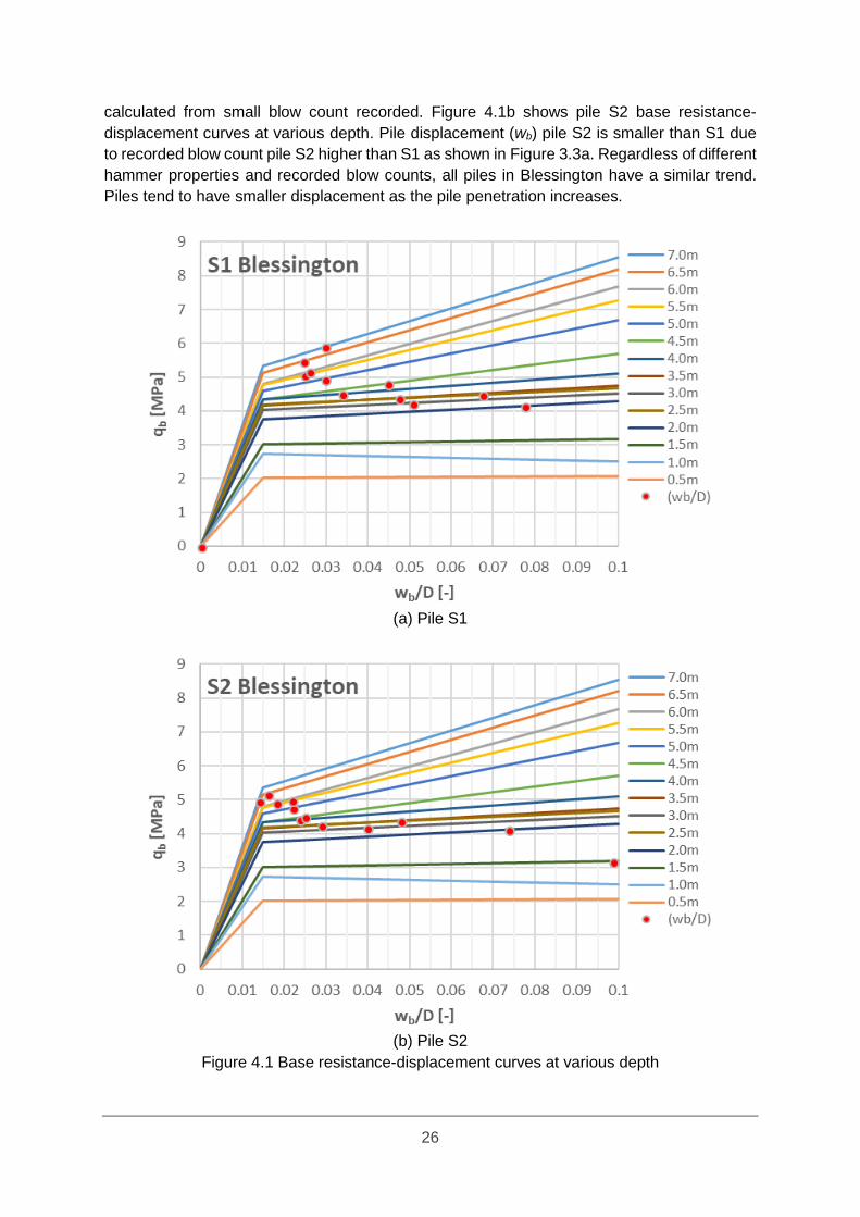
Figure 4.1 shows the base resistance-displacement curve at various depth. In the first linear
part, at wb/D < 0.015, the qb - wb/D curves are increased mirroring soil elastic stiffness (Eo)
value which increases along the pile depth. The base resistance value from the UWA-05
approach (𝑞𝑏01,𝑈𝑊𝐴) is used as a limit when wb greater than the failure criteria of 0.1 of pile
diameter (D). The pile tip displacement normalises by the pile diameter (wb/D) during the pile
driving are shown in the red dot. Almost all wb/D occur at the second linear stage between
0.015 and 0.1. The wb/D are decreased as the blow counts increased at deeper pile
penetration. The wb during driving less than failure criteria of 0.1D except for the first meter
when the pile is fully coring (IFR=1).
Figure 4.1a shows the base resistance - displacement curves for pile S1 at various depth. It
can be observed that at 0.5m, qb - wb/D equal to zero correspond to zero recorded blow count
at this depth. Zero blow count can be an indication of self-weight penetration occurrence at
0.5m depth. Although pile self-weight calculation indicates no self-weight penetration in
Blessington site, ignoring equipment weight can be the reason zero blow count record occurs
at a depth near the surface. At 1-1.5m depth, wb value is higher than 0.1D due to back-
26
calculated from small blow count recorded. Figure 4.1b shows pile S2 base resistance-
displacement curves at various depth. Pile displacement (wb) pile S2 is smaller than S1 due
to recorded blow count pile S2 higher than S1 as shown in Figure 3.3a. Regardless of different
hammer properties and recorded blow counts, all piles in Blessington have a similar trend.
Piles tend to have smaller displacement as the pile penetration increases.
(a) Pile S1
(b) Pile S2
Figure 4.1 Base resistance-displacement curves at various depth
27
4.2 Static Capacity Approach Comparison
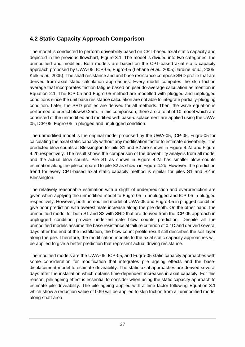
The model is conducted to perform driveability based on CPT-based axial static capacity and
depicted in the previous flowchart, Figure 3.1. The model is divided into two categories, the
unmodified and modified. Both models are based on the CPT-based axial static capacity
approach proposed by UWA-05, ICP-05, Fugro-05 (Lehane et al., 2005; Jardine et al., 2005;
Kolk et al., 2005). The shaft resistance and unit base resistance compose SRD profile that are
derived from axial static calculation approaches. Every model computes the skin friction
average that incorporates friction fatigue based on pseudo-average calculation as mention in
Equation 2.1. The ICP-05 and Fugro-05 method are modelled with plugged and unplugged
conditions since the unit base resistance calculation are not able to integrate partially-plugging
condition. Later, the SRD profiles are derived for all methods. Then, the wave equation is
performed to predict blows/0.25m. In this comparison, there are a total of 10 model which are
consisted of the unmodified and modified with base-displacement are applied using the UWA-
05, ICP-05, Fugro-05 in plugged and unplugged condition.
The unmodified model is the original model proposed by the UWA-05, ICP-05, Fugro-05 for
calculating the axial static capacity without any modification factor to estimate driveability. The
predicted blow counts at Blessington for pile S1 and S2 are shown in Figure 4.2a and Figure
4.2b respectively. The result shows the comparison of the driveability analysis from all model
and the actual blow counts. Pile S1 as shown in Figure 4.2a has smaller blow counts
estimation along the pile compared to pile S2 as shown in Figure 4.2b. However, the prediction
trend for every CPT-based axial static capacity method is similar for piles S1 and S2 in
Blessington.
The relatively reasonable estimation with a slight of underprediction and overprediction are
given when applying the unmodified model to Fugro-05 in unplugged and ICP-05 in plugged
respectively. However, both unmodified model of UWA-05 and Fugro-05 in plugged condition
give poor prediction with overestimate increase along the pile depth. On the other hand, the
unmodified model for both S1 and S2 with SRD that are derived from the ICP-05 approach in
unplugged condition provide under-estimate blow counts prediction. Despite all the
unmodified models assume the base resistance at failure criterion of 0.1D and derived several
days after the end of the installation, the blow count profile result still describes the soil layer
along the pile. Therefore, the modification models to the axial static capacity approaches will
be applied to give a better prediction that represent actual driving resistance.
The modified models are the UWA-05, ICP-05, and Fugro-05 static capacity approaches with
some consideration for modification that integrates pile ageing effects and the base-
displacement model to estimate driveability. The static axial approaches are derived several
days after the installation which obtains time-dependent increases in axial capacity. For this
reason, pile ageing effect is essential to consider when using the static capacity approach to
estimate pile driveability. The pile ageing applied with a time factor following Equation 3.1
which show a reduction value of 0.69 will be applied to skin friction from all unmodified model
along shaft area.
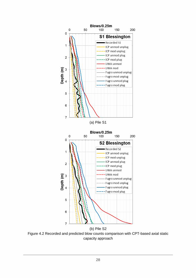
28
(a) Pile S1
(b) Pile S2
Figure 4.2 Recorded and predicted blow counts comparison with CPT-based axial static
capacity approach
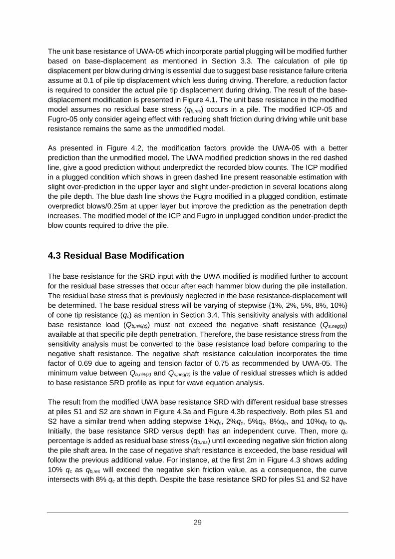
29
The unit base resistance of UWA-05 which incorporate partial plugging will be modified further
based on base-displacement as mentioned in Section 3.3. The calculation of pile tip
displacement per blow during driving is essential due to suggest base resistance failure criteria
assume at 0.1 of pile tip displacement which less during driving. Therefore, a reduction factor
is required to consider the actual pile tip displacement during driving. The result of the base-
displacement modification is presented in Figure 4.1. The unit base resistance in the modified
model assumes no residual base stress (qb,res) occurs in a pile. The modified ICP-05 and
Fugro-05 only consider ageing effect with reducing shaft friction during driving while unit base
resistance remains the same as the unmodified model.
As presented in Figure 4.2, the modification factors provide the UWA-05 with a better
prediction than the unmodified model. The UWA modified prediction shows in the red dashed
line, give a good prediction without underpredict the recorded blow counts. The ICP modified
in a plugged condition which shows in green dashed line present reasonable estimation with
slight over-prediction in the upper layer and slight under-prediction in several locations along
the pile depth. The blue dash line shows the Fugro modified in a plugged condition, estimate
overpredict blows/0.25m at upper layer but improve the prediction as the penetration depth
increases. The modified model of the ICP and Fugro in unplugged condition under-predict the
blow counts required to drive the pile.
4.3 Residual Base Modification
The base resistance for the SRD input with the UWA modified is modified further to account
for the residual base stresses that occur after each hammer blow during the pile installation.
The residual base stress that is previously neglected in the base resistance-displacement will
be determined. The base residual stress will be varying of stepwise {1%, 2%, 5%, 8%, 10%}
of cone tip resistance (qc) as mention in Section 3.4. This sensitivity analysis with additional
base resistance load (Qb,n%(z)) must not exceed the negative shaft resistance (Qs,neg(z))
available at that specific pile depth penetration. Therefore, the base resistance stress from the
sensitivity analysis must be converted to the base resistance load before comparing to the
negative shaft resistance. The negative shaft resistance calculation incorporates the time
factor of 0.69 due to ageing and tension factor of 0.75 as recommended by UWA-05. The
minimum value between Qb,n%(z) and Qs,neg(z) is the value of residual stresses which is added
to base resistance SRD profile as input for wave equation analysis.
The result from the modified UWA base resistance SRD with different residual base stresses
at piles S1 and S2 are shown in Figure 4.3a and Figure 4.3b respectively. Both piles S1 and
S2 have a similar trend when adding stepwise 1%qc, 2%qc, 5%qc, 8%qc, and 10%qc to qb.
Initially, the base resistance SRD versus depth has an independent curve. Then, more qc
percentage is added as residual base stress (qb,res) until exceeding negative skin friction along
the pile shaft area. In the case of negative shaft resistance is exceeded, the base residual will
follow the previous additional value. For instance, at the first 2m in Figure 4.3 shows adding
10% qc as qb,res will exceed the negative skin friction value, as a consequence, the curve
intersects with 8% qc at this depth. Despite the base resistance SRD for piles S1 and S2 have

30
a similar trend when adding base resistance stresses, pile S1 has higher base resistance SRD
profile than pile S2.
(a) Pile S1 (b) Pile S2
Figure 4.3 UWA unit base resistance with varying residual base stresses added
Figure 4.4a and Figure 4.4b illustrate the blow count prediction when residual base stresses
are incorporated at pile S1 and pile S2 respectively. These figures also present the recorded
blow counts as a reference for the comparison to blow count prediction. Reversely with base
resistance SRD profile as shown in Figure 4.3, pile S2 has a higher blow counts prediction
compare to pile S1 as shown in Figure 4.4. This is due to pile S1 has higher hammer stroke
than pile S1.
Figure 4.4 highlights that the UWA modified without additional base residual stresses is
closest to the actual blow counts profile along the pile length. However, without additional
base residual stresses, pile S1 and S2 still have underpredicted at 5.25m and 6.25m
respectively. Adding the residual base stresses lead to higher prediction at piles S1-S2. The
reasonable blow count estimation without underprediction is provided by adding 5% qc and
2% qc at pile S1 and S2 accordingly.
31
(a) Pile S1 (b) Pile S2
Figure 4.4 Recorded and predicted blow count with residual base stresses added
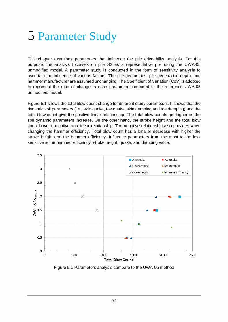
32
5 Parameter Study
This chapter examines parameters that influence the pile driveability analysis. For this
purpose, the analysis focusses on pile S2 as a representative pile using the UWA-05
unmodified model. A parameter study is conducted in the form of sensitivity analysis to
ascertain the influence of various factors. The pile geometries, pile penetration depth, and
hammer manufacturer are assumed unchanging. The Coefficient of Variation (CoV) is adopted
to represent the ratio of change in each parameter compared to the reference UWA-05
unmodified model.
Figure 5.1 shows the total blow count change for different study parameters. It shows that the
dynamic soil parameters (i.e., skin quake, toe quake, skin damping and toe damping) and the
total blow count give the positive linear relationship. The total blow counts get higher as the
soil dynamic parameters increase. On the other hand, the stroke height and the total blow
count have a negative non-linear relationship. The negative relationship also provides when
changing the hammer efficiency. Total blow count has a smaller decrease with higher the
stroke height and the hammer efficiency. Influence parameters from the most to the less
sensitive is the hammer efficiency, stroke height, quake, and damping value.
Figure 5.1 Parameters analysis compare to the UWA-05 method

33
5.1. Damping
Damping value influences the driveability analysis as shown in the blow count result. The
damping value depends solely on the soil type. Damping value in the sand layer suggested
by the UWA-05 method is 0.25s/m and 0.5s/m respectively for skin and toe. Figure 5.2 shows
that the sensitivity analysis with changing the toe damping give greater blows than changing
the skin damping. The effect of changing the damping parameter is not constant along the pile
but increase as the pile depth increases. At the pile base, an increase of 50% of the skin and
toe damping provide increased blows of 1.1 and 1.2 respectively. Generally, the blow counts
and damping value are positively correlated. The blow counts are increased with increased
damping value. Soil damping in the wave equation analysis represents the energy loss within
the soil in the pile-soil interface during the pile driving process. Hence, higher damping value
means more energy lost and more blow count required for pile driving.
(a) Skin damping (b) Toe damping
Figure 5.2 Effect of damping
5.2. Quake
Quake is the maximum displacement to achieve yield. Increasing the quake value causes
extension of the soil elastic displacement range before yield and decreases the soil stiffness.
The quake value suggested by the UWA-05 method is 2.5mm both for the skin and toe. The
blow count result is influenced by the quake value as shown in Figure 5.3. The toe quake has
less influence on the result blow count than the skin quake. The blow count increase due to

34
the quake value is developed along the pile penetration depth. At 7m depth, 50% increase in
the quake value give increase blows/0.25m of 1.4 and 1.3 for changing the skin and toe quake
accordingly. The quake value in wave equation analysis input does not represent pile
displacement rather than marking the yield displacement point in the soil resistance-pile
displacement curve (Figure 2.5). Changing the quake value will move the yield displacement
point and enlarge the linear relationship of soil resistance-pile displacement. Thus, higher
quake causes more blow count is required to install the pile. The effect of changing the quake
value similar to the damping, the blow counts are increased with increased quake value.
Although, the blow count increases due to the quake value slightly higher than the blow count
increase due to the damping value.
(a) Skin quake (b) Toe quake
Figure 5.3 Effect of quake
5.3. Stroke Height
The height of hammer stroke influences the energy applied to drive a pile. Figure 5.4a shows
the blow count/0.25m resulting from varying the hammer stroke height. The blow count and
stroke height have a non-linear negative relationship. The blow count at the pile tip decreases
by a factor of 0.38 when the hammer stroke height increases from 0.3m to 0.45m, as shown
in the red line and the light blue line respectively. This non-linear relationship is shown in the
graph when increasing the stroke height with the same increment of 0.15m, from 0.45m to
0.6m, the blow count at the pile base decrease by a factor of 0.65. Increase in the stroke
height causes higher energy to drive a pile or decrease blow count required to install the pile.

35
The hammer stroke height must be carefully assessed. Installing pile with excessive energy
prone to cause pile damage. In another hand, pile driving using low stroke lead to premature
refusal. Therefore, as an addition to blow count prediction, the stress along the pile must be
considered when adjusting the hammer stroke height.
5.4. Hammer Efficiency
Hammer efficiency accounts for the energy losses that cannot be calculated during the pile
driving process. The standard value of the hammer efficiency depends on the type of hammer.
The pile S2 installation process at Blessington site uses a hydraulic impact hammer. This type
of hammer has hammer efficiency value of 0.8 following the GRLWEAP recommendation.
Figure 5.4b shows that hammer efficiency gives a negative correlation with the blow count
result. The blow count is increasing as the hammer efficiency decrease. The change in the
blow count increase toward the pile base. The blow count at the pile base increases by a
factor of 1.72 while the hammer efficiency decrease from 0.8 to 0.7. More efficient hammer
provides higher energy cause lower blow count required to install the pile. The effect of
changing hammer efficiency gives the highest change in the blow count result compare to
other parameters in this study. Therefore, it is crucial to ensure the hammer efficiency design
match to actual hammer efficiency, so that the blow count prediction can represent the actual
driving process.
Figure 5.4 Effect of (a) stroke height (b) hammer efficiency
36
6 Case Study – Rotterdam Harbour
This chapter presents a case study of pile installation in Rotterdam Harbour. The input data
from the Rotterdam site will be presented. The driveability models that have been developed
for Blessington site is applied at Rotterdam site. The primary input for the SRD calculation will
incorporate several aspects such as the ageing effect, the degree of displacement and
residual base stresses. The result of various models CPT-based axial static capacity
approaches are discussed.
6.1. Database at Rotterdam
The project undertakes 4 full-scale test piles at Rotterdam Harbour, the Netherlands. The test
location is comprised of clay with organic soil, and medium dense sand. A total of 10 CPTs
were conducted at Rotterdam site. Figure 6.1a describes the cone tip resistance (qc) profiles
indicate that low qc (< 2MPa) in the clay layer from 4m to 21m. The soil shear modulus (Go)
profiles were derived from the 6qc values since the shear wave velocity (Vs) are unknown
(Prendergast et al., 2013). These Go profiles are derived from the qc value are shown in Figure
6.1b. Poisson’s ratio (ν) at a very small strain of 0.1 is used as an assumption in this project.
Piles P1-P4 have the identical properties, square close-ended concrete piles with 0.45m width.
The total pile length of 36m is driven until 35m below ground level. Blow count records at
Rotterdam for all piles are plotted in Figure 6.1c. The incremental blow counts are recorded
over the last 5m of pile driving, from 30 to 35m depth. Freefall occurs only over a minor length,
but in the principal, the hammer is worked over the entire length of the pile. All the blow counts
record has a similar profile which ranges around 10 blows/0.25m and increases at the last 1m
near the pile tip.
The blow counts record at Rotterdam are directly comparable since the piles had the same
hammers and stroke heights. Pile is driven using 6200kg Delmag D62-22 as a piling hammer.
The hammer blow energy ranges between 107 and 224 kNm. The stroke height of 1.7m is
determined from the minimum hammer blow energy of 107 kNm. Pile cushion consists of three
layers of spruce. There is no available data about the thickness of the pile cushion, thus this
study will assumes cushion thickness is 0.1m according to the minimum required pile cushion
thickness for the concrete pile (PDCA, 2007).
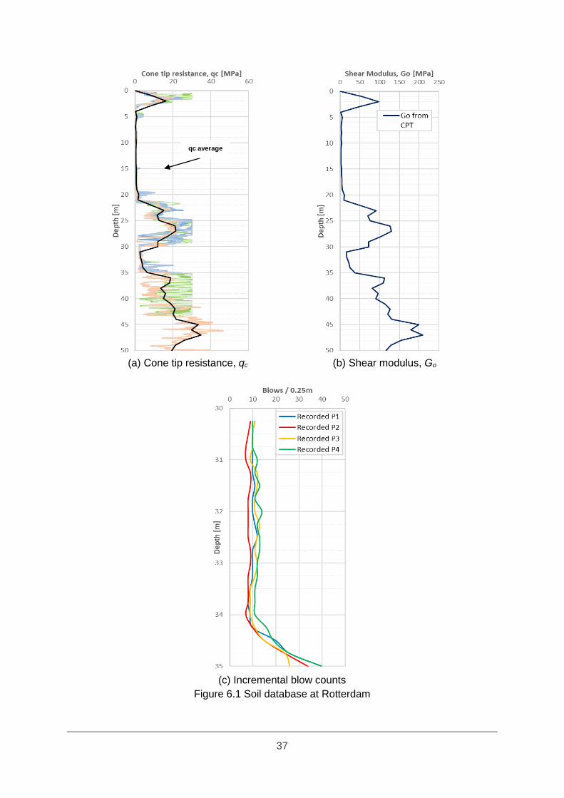
37
(a) Cone tip resistance, qc (b) Shear modulus, Go
(c) Incremental blow counts
Figure 6.1 Soil database at Rotterdam
qc average
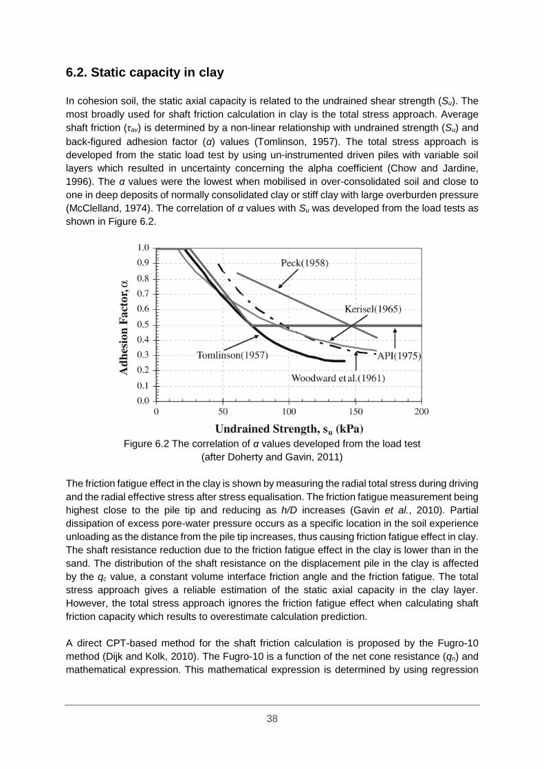
38
6.2. Static capacity in clay
In cohesion soil, the static axial capacity is related to the undrained shear strength (Su). The
most broadly used for shaft friction calculation in clay is the total stress approach. Average
shaft friction (τav) is determined by a non-linear relationship with undrained strength (Su) and
back-figured adhesion factor (α) values (Tomlinson, 1957). The total stress approach is
developed from the static load test by using un-instrumented driven piles with variable soil
layers which resulted in uncertainty concerning the alpha coefficient (Chow and Jardine,
1996). The α values were the lowest when mobilised in over-consolidated soil and close to
one in deep deposits of normally consolidated clay or stiff clay with large overburden pressure
(McClelland, 1974). The correlation of α values with Su was developed from the load tests as
shown in Figure 6.2.
Figure 6.2 The correlation of α values developed from the load test
(after Doherty and Gavin, 2011)
The friction fatigue effect in the clay is shown by measuring the radial total stress during driving
and the radial effective stress after stress equalisation. The friction fatigue measurement being
highest close to the pile tip and reducing as h/D increases (Gavin et al., 2010). Partial
dissipation of excess pore-water pressure occurs as a specific location in the soil experience
unloading as the distance from the pile tip increases, thus causing friction fatigue effect in clay.
The shaft resistance reduction due to the friction fatigue effect in the clay is lower than in the
sand. The distribution of the shaft resistance on the displacement pile in the clay is affected
by the qc value, a constant volume interface friction angle and the friction fatigue. The total
stress approach gives a reliable estimation of the static axial capacity in the clay layer.
However, the total stress approach ignores the friction fatigue effect when calculating shaft
friction capacity which results to overestimate calculation prediction.
A direct CPT-based method for the shaft friction calculation is proposed by the Fugro-10
method (Dijk and Kolk, 2010). The Fugro-10 is a function of the net cone resistance (qn) and
mathematical expression. This mathematical expression is determined by using regression
39
analysis to explore the lowest coefficient of variation to measure the pile capacity. Before using
Fugro-10, the cone tip resistance (qc) needed to be converted to the total cone resistance (qt)
by using a simplified correlation which is suggested in Lehane et al. (2017) as shown in Table
6.1. The Fugro-10 shaft friction calculation is influenced by over-consolidation and pile length,
instead of by load direction, soil plasticity, pile diameter, and pile tip displacement. The Fugro-
10 method incorporates the friction fatigue effect in the shaft resistance calculation as
represented by the relative depth to the pile tip normalised by the unit length (h/uL). This
incorporation gives closer and less conservative representation of the actual condition.
The Fugro-10 unit base resistance is calculated average qn of 1.5 diameters above and below
the penetration. This approach is derived according to the principles of the CPT-based
methods that is proposed by API-00 for the sand layer. The API-00 proposed calculating the
unit base resistance in weak clay layer with an assumption of the pile tip penetrate more into
the layer in question approximately 3 diameters above the bottom of the layer to preclude
punch through (API, 2007). The axial shaft capacity calculation approaches for the driven pile
in the clay which are used in this study are shown in Table 6.1.
6.3. Blow Count Prediction
The database of full-scale test piles at Rotterdam is used as the input for the driveability
analysis. In this section, the pile P1 is taken as a representative pile since all piles have
identical pile and hammer properties. The other Rotterdam piles result analysis are summaries
in the Appendix C. The soil properties in this project consist of clay, organic soil and sand
layer. Therefore, the SRD profile is determined by a combination of several approaches. The
first combination is the UWA model by using the UWA-05 in sand, total stress approach and
API-00 in clay. The second combination is the ICP model by using the ICP-05 in sand with
total stress and API-00 in clay. The last combination is Fugro model using the Fugro-05 in
sand and Fugro-10 in clay.
Like Blessington site, the base resistance–displacement modification is applied to the
combination with UWA as mentioned in Section 3.3. The residual base stresses in this
modification assume to be zero. The actual displacements (wb) for each blow are back-
calculated from the blow count recorded at Rotterdam pile. Later, the actual displacement is
normalised by the pile diameter (D). The base resistance-displacement curve first stage is
linear until it reaches a yield strain of 0.015D. At this point, the second linear stage is formed
until 0.1D.
At Rotterdam project, the blow counts are recorded only the last 5m at the final driving.
Therefore, only the actual displacement at 30-35m can be determined by back-calculated the
record blow count. Soil at this depth consists of clay layer with qc between 2 and 6 MPa. Since
the recorded blow count is located in the clay layer, the unit base resistance is applied using
the API-00 approach while the shaft friction is applied using the total stress approach.
Figure 6.3 shows the base resistance-displacement curve when applying a simplified three-
stage base resistance-displacement as suggested by Gavin and Lehane (2007). In the first
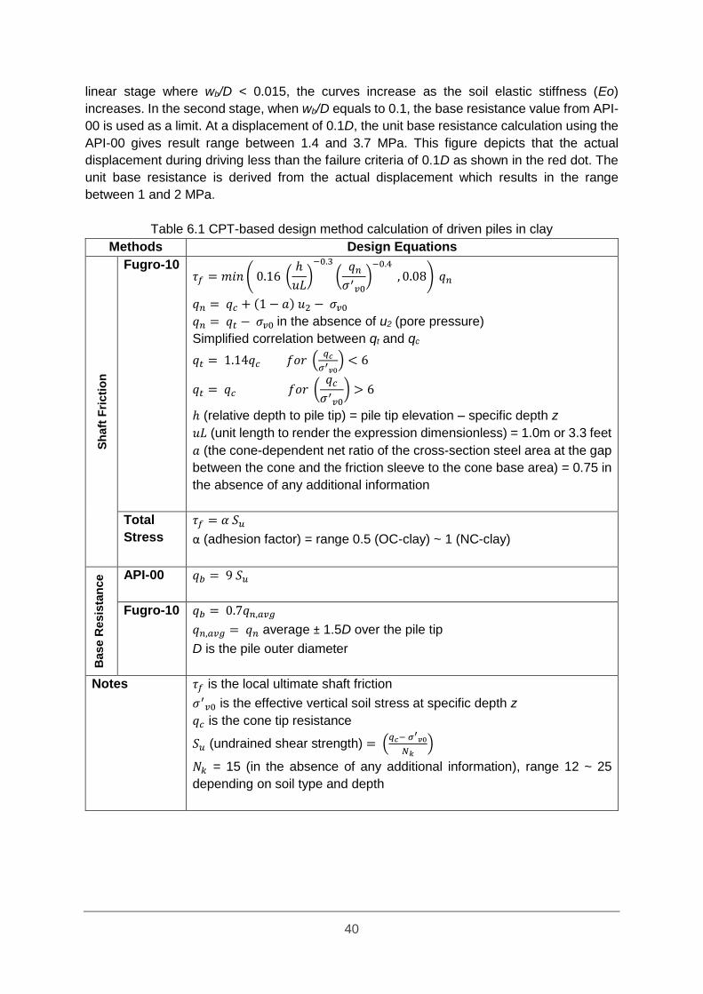
40
linear stage where wb/D < 0.015, the curves increase as the soil elastic stiffness (Eo)
increases. In the second stage, when wb/D equals to 0.1, the base resistance value from API-
00 is used as a limit. At a displacement of 0.1D, the unit base resistance calculation using the
API-00 gives result range between 1.4 and 3.7 MPa. This figure depicts that the actual
displacement during driving less than the failure criteria of 0.1D as shown in the red dot. The
unit base resistance is derived from the actual displacement which results in the range
between 1 and 2 MPa.
Table 6.1 CPT-based design method calculation of driven piles in clay
Methods Design Equations
Sh
aft
Fri
cti
on
Fugro-10 𝜏𝑓 = 𝑚𝑖𝑛 ( 0.16 (
ℎ
𝑢𝐿)
−0.3
( 𝑞𝑛
𝜎′𝑣0
)−0.4
, 0.08) 𝑞𝑛
𝑞𝑛 = 𝑞𝑐 + (1 − 𝑎) 𝑢2 − 𝜎𝑣0
𝑞𝑛 = 𝑞𝑡 − 𝜎𝑣0 in the absence of u2 (pore pressure)
Simplified correlation between qt and qc
𝑞𝑡 = 1.14𝑞𝑐 𝑓𝑜𝑟 (𝑞𝑐
𝜎′𝑣0
) < 6
𝑞𝑡 = 𝑞𝑐 𝑓𝑜𝑟 (𝑞𝑐
𝜎′𝑣0
) > 6
ℎ (relative depth to pile tip) = pile tip elevation – specific depth z
𝑢𝐿 (unit length to render the expression dimensionless) = 1.0m or 3.3 feet
𝑎 (the cone-dependent net ratio of the cross-section steel area at the gap
between the cone and the friction sleeve to the cone base area) = 0.75 in
the absence of any additional information
Total
Stress
𝜏𝑓 = 𝛼 𝑆𝑢
α (adhesion factor) = range 0.5 (OC-clay) ~ 1 (NC-clay)
Base R
esis
tan
ce
API-00 𝑞𝑏 = 9 𝑆𝑢
Fugro-10 𝑞𝑏 = 0.7𝑞𝑛,𝑎𝑣𝑔
𝑞𝑛,𝑎𝑣𝑔 = 𝑞𝑛 average ± 1.5D over the pile tip
D is the pile outer diameter
Notes 𝜏𝑓 is the local ultimate shaft friction
𝜎′𝑣0 is the effective vertical soil stress at specific depth z
𝑞𝑐 is the cone tip resistance
𝑆𝑢 (undrained shear strength) = (𝑞𝑐− 𝜎′
𝑣0
𝑁𝑘)
𝑁𝑘 = 15 (in the absence of any additional information), range 12 ~ 25
depending on soil type and depth
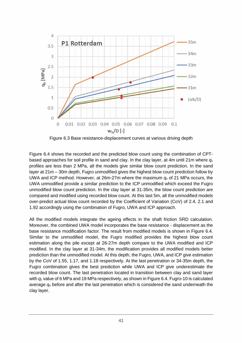
41
Figure 6.3 Base resistance-displacement curves at various driving depth
Figure 6.4 shows the recorded and the predicted blow count using the combination of CPT-
based approaches for soil profile in sand and clay. In the clay layer, at 4m until 21m where qc
profiles are less than 2 MPa, all the models give similar blow count prediction. In the sand
layer at 21m – 30m depth, Fugro unmodified gives the highest blow count prediction follow by
UWA and ICP method. However, at 26m-27m where the maximum qc of 21 MPa occurs, the
UWA unmodified provide a similar prediction to the ICP unmodified which exceed the Fugro
unmodified blow count prediction. In the clay layer at 31-35m, the blow count prediction are
compared and modified using recorded blow count. At this last 5m, all the unmodified models
over-predict actual blow count recorded by the Coefficient of Variation (CoV) of 2.4, 2.1 and
1.92 accordingly using the combination of Fugro, UWA and ICP approach.
All the modified models integrate the ageing effects in the shaft friction SRD calculation.
Moreover, the combined UWA model incorporates the base resistance - displacement as the
base resistance modification factor. The result from modified models is shown in Figure 6.4.
Similar to the unmodified model, the Fugro modified provides the highest blow count
estimation along the pile except at 26-27m depth compare to the UWA modified and ICP
modified. In the clay layer at 31-34m, the modification provides all modified models better
prediction than the unmodified model. At this depth, the Fugro, UWA, and ICP give estimation
by the CoV of 1.55, 1.17, and 1.18 respectively. At the last penetration or 34-35m depth, the
Fugro combination gives the best prediction while UWA and ICP give underestimate the
recorded blow count. The last penetration located in transition between clay and sand layer
with qc value of 6 MPa and 19 MPa respectively, as shown in Figure 6.4. Fugro-10 is calculated
average qn before and after the last penetration which is considered the sand underneath the
clay layer.

42
The base resistance for combined UWA by using UWA-05 in the sand, the total stress
approach and API-00 in clay are modified further to account for the residual base stresses.
The residual base stresses occur after each hammer blow during pile installation. In this
modification, the model has integrated not only the base resistance-displacement but also the
residual base stresses. The residual base stress is cooperated with adding {1, 2,5,8,10}% of
the cone tip resistance (qc) to the unit base stress as mentioned in Section 3.4. The additional
base residual must less than the negative shaft resistance available at the specific pile depth
penetration. Like Blessington model, the Rotterdam model takes the time factor of 0.69 due
to the ageing effect and a tension factor of 0.75 as a recommended by the UWA-05. The time
factor and tension capacity are used when calculating the negative shaft resistance. After
ensuring that base resistance load less than the negative shaft resistance, the SRD profile for
the UWA modified including base resistance residual are derived.
Figure 6.4 Predicted blow counts comparison using CPT-based approaches at pile P1
Figure 6.5 presents the result of modified UWA base resistance with varying residual stresses
at Rotterdam. Whether the residual stress is added in the base resistance is depends on the
magnitude of qc at each layer. The small qc values in the clay layer at 4 until 21m depth and
31 until 35m lead to an insignificant addition to the base resistance SRD. In the sand layer,
for instance at 26m when the maximum cone tip resistance equals to 21 MPa, noticeable
change in the base resistance SRD result is observed due to adding base residual stresses.
The base resistance SRD profile is updated after adding the residual base stress value. Then,
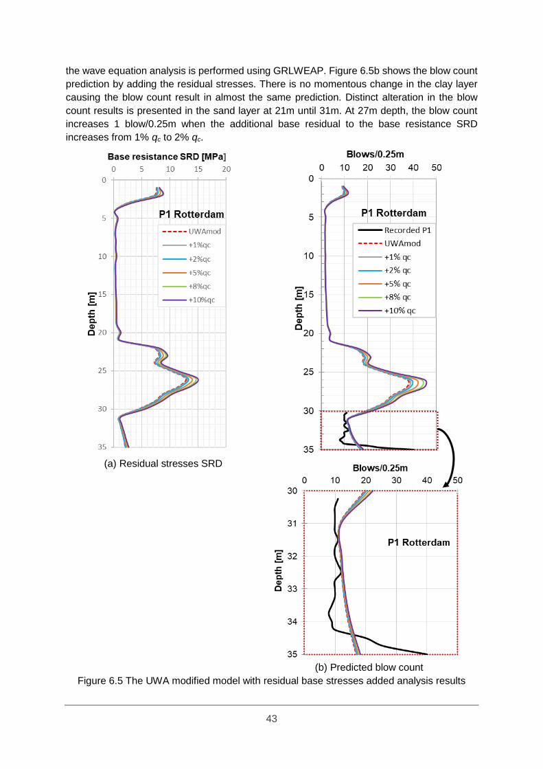
43
the wave equation analysis is performed using GRLWEAP. Figure 6.5b shows the blow count
prediction by adding the residual stresses. There is no momentous change in the clay layer
causing the blow count result in almost the same prediction. Distinct alteration in the blow
count results is presented in the sand layer at 21m until 31m. At 27m depth, the blow count
increases 1 blow/0.25m when the additional base residual to the base resistance SRD
increases from 1% qc to 2% qc.
(a) Residual stresses SRD
(b) Predicted blow count
Figure 6.5 The UWA modified model with residual base stresses added analysis results

44
Driveability analysis performance by using the CPT-based axial static capacity approaches in
combine sand-clay layer with modification model provide a better prediction than the
unmodified model. All modified models are addressing the ageing and the friction fatigue effect
in the shaft friction SRD profile. The combine UWA model (UWA-05 in sand, total stress
approach and API-00 in clay) is modified further by addressing the degree of mobilisation and
the residual base stresses. The combine UWA without additional base resistance is provided
the closest blow count prediction to the actual blow count except in the last depth penetration.
The upper prediction cannot be verified due to record blow count is only available at the last
5m.
45
7 Conclusions and
Recommendation
The primary focus of the research is to gain knowledge on the performance of the CPT-based
axial static capacity approaches to evaluate pile driveability in sand. A literature study to
determine the pile driveability from the axial static capacity is conducted. Then, the site
database including the site condition, hammer and pile properties will be compiled as the
inputs to perform the wave equation analysis. Several factors concerning driveability analysis
are addressed to develop an efficient model. Finally, the blow count results from every model
are assessed. To be able to achieve the primary focus of this research, the answer to sub-
question is listed as follows:
1. How to calculate the axial static capacity using available CPT-based methods?
This study uses several approaches to calculate the CPT-based axial static capacity (i.e. the
UWA-05, ICP-05, and Fugro-05). These axial static approaches address the friction fatigue
effect when computing the shaft resistance capacity in a pile which is represented in the ICP-
05 and Fugro-05 by h/R* and in the UWA-05 method by h/D. The friction fatigue effect causes
a reduction in the shaft resistance as the distance from the pile tip to the specific soil horizon
increases. All the approaches consider plugging condition in the unit base resistance
calculation. However, only the UWA-05 method considers partial plugging conditions in the
calculation approach, which is accounted for in the shaft friction and the unit base resistance
by IFR and FFR respectively. The ICP-05 and Fugro-05 take conservatively the fully plugged
or unplugged condition in the unit base resistance calculation.
2. How to develop an efficient model for the driveability analysis using the CPT-based
axial capacity methods?
Soil resistance during driving is a combination of static and dynamic components of the soil.
The static resistance to driving (SRD) is analogous with the static axial capacity but
incorporates base resistance for each driving increment (as opposed to static capacity which
has only one base resistance). The axial static capacity methods are derived from the axial
static piles load test database. Therefore, in developing a driveability analysis, several factors
must be carefully evaluated. The dynamic components which affect the soil resistance during
driving are the soil damping and quake. Driveability analysis integrates both the static and
dynamic components in the wave equation analysis. Inputs needed to perform the wave
equation analysis are the SRD and dynamic soil components, the pile and hammer properties.
The driveability analysis is applied to calculate the blow count for each depth increment.
The first factor that affects the driveability analysis is the friction fatigue effect that occurs for
each driving increment. Thus, the pseudo average shaft friction calculation is implemented in
the shaft resistance SRD to calculate the change in the shaft resistance distribution between
two successive depth increments. The second factor that needs to be considered is the pile
46
ageing effect in a pile. The CPT-based axial static capacity approaches are derived 10-30
days after the pile installation. A time-dependent increase in the static axial capacity is
observed for the driven piles in sand. Therefore, a time factor of 0.69 is applied to quantify the
magnitude of shaft resistance reduction when performing the driveability study with the axial
static capacity approaches.
The base resistance-displacement curves are determined by back-calculating the actual blow
counts record to establish the degree of soil displacement during driving. The actual
displacement from the base-displacement curves are applied to the unit base resistance using
the UWA-05 approach. These curves indicated soil displacement during driving less than the
assumption of the pile tip displacement suggested by the UWA-05 methods of 0.1 of the pile
diameter. As a consequence, the unit base resistance SRD inputs less than the unit base
resistance calculation using the UWA-05 approach.
During pile driving, the pile will experience compression when the driving force from the
hammer is applied and tension when the pile is unloaded. At zero pile loading, the residual
base stress occurs at the pile base. The sensitivity study analysis to account for the residual
base stresses are conducted with an additional {1; 2; 5; 8; 10} % of the cone tip resistance.
This sensitivity analysis with additional base resistance load must not exceed the negative
shaft resistance available at that specific pile depth penetration. The negative shaft resistance
calculation incorporates the pile ageing effect and tension factor of 0.75 as recommended by
the UWA-05 approach. The minimum value between the base resistance load and the
negative shaft resistance is the value of residual stresses which is added to base resistance
SRD profile as input for wave equation analysis.
3. What parameters primarily affect pile driveability analysis?
The parameter study is conducted using sensitivity analysis for the dynamic soil component
and hammer properties. The dynamic soil components are used in this study based on the
UWA-05 recommendation value for steel pile driven in the sand. Therefore, to aim efficient
model for analysis, the influence of these dynamic soil parameters must be assessed. The
result of the hammer properties sensitivity analysis must be considered when selecting
equipment for driving a pile. From all the sensitivity analysis of parameters result can be
concluded that the most influential factor that determines blow count is the hammer efficiency.
Influence parameters followed by the stroke height, quake, and damping value. Blow count
will increase related to lower hammer efficiency, lower stroke height, higher quake and higher
damping.
Finally, the aim of this research can be concluded. Performing unmodified axial static capacity
approaches give an unreasonable prediction. The raw model of the ICP-05 and Fugro-05 are
taken conservative plugging condition. These two approaches give over-predict blow count
estimation in the fully plugging pile base condition. In another hand, the ICP-05 and Fugro-05
unmodified in the unplugged pile base condition provide under estimate blow count prediction.
Under-predict blow count result is highly avoided in the driveability analysis. The UWA-05
unmodified also give unreasonable over-prediction despite including the partially plugging
effect in the base resistance calculation.
47
Performing driveability analysis using the CPT-based axial static capacity approaches (i.e.,
UWA-05, ICP-05, Fugro-05) with modification model provide a better prediction. However,
integrating the friction fatigue effect and the pile ageing effect into the Fugro-05 approach still
produces over-predictions in blow counts along the pile. The ICP-05 modified give reasonable
prediction with slight under-predictions in several locations along the pile length. Model using
the UWA-05 modified further addressing the degree of mobilisation and base residual stresses
provide reasonable blow count prediction. This UWA-05 modified model can be recognised
as an exemplary model to estimate the blow counts from the CPT-based axial static capacity
approach.
Conducting driveability analysis study with a complete record blow count along the pile is
complimentary. The recorded blow counts not only for actual displacement calculation and
model modification but also as the model validation. The model validation will make the
analysis result become more reliable. Beside recorded blow count, the completeness of
hammer driving equipment data is favourable. As the hammer properties profoundly affect the
driveability analysis, using complete hammer properties make more confident blow count
prediction which represent the actual blow count during pile installation.
Driveability analysis is essential to consider the driving stresses and installation time as an
addition to blow count prediction. Considering maximum driving force during pile installation
can prevent the pile material damage. Knowing the pile installation time give an advantage in
project scheduling, especially when a large number of piles need to be installed. The
driveability analysis considering these aspects will ensure the pile quality, time-frame and
budget according to the plan. More research to perform driveability analysis that considers
these aspects will be beneficial for driveability analysis.
48
Bibliography
Alawneh, A. S. and Husein Malkawi, A. I. (2000) ‘Estimation of Post-Driving Residual
Stresses Along Driven Piles in Sand’, Geotechnical Testing Journal, 23(3), pp. 313–326.
doi: 10.1520/GTJ11053J.
Alm, T. and Hamre, L. (2001) ‘Soil model for pile driveability predictions based on CPT
interpretations’, International Conference on Soil Mechanics and Geotechnical
Engineering, pp. 1297–1302. Available at:
http://scholar.google.com/scholar?hl=en&btnG=Search&q=intitle:Soil+model+for+pile+dri
veability+predictions+based+on+CPT+interpretations#0.
API (2007) ‘Recommended Practice for Planning, Designing and Constructing Fixed
Offshore Platforms — Working Stress Design’, Api Recommended Practice, 24–
WSD(December 2000), p. 242. doi: 10.1007/s13398-014-0173-7.2.
Byrne, T. et al. (2012) ‘Comparison of Pile Driveability Methods In North Sea Sand’,
Offshore Site Investigation and Geotechnics: Integrated Technologies - Present and
Future. doi: SUT-OSIG-12-52.
Byrne, T. et al. (2018) Performance of CPT-based methods to assess monopile driveability
in North Sea sands. Ocean Engineering (In Review).
Chauhan, S. (2008) Pile Design Using Wave Equation Analysis Program Application in
Offshore Wind Farm. Massachusetts Institute of Technology.
Chow, F. C. and Jardine, R. J. (1996) Investigations into the behaviour of displacement piles
for offshore foundations, Ground Engineering. Imperial College London.
Das, B. M. (2011) Principles of Foundation Engineering. Seventh Ed. Cengage Learning,
USA. Available at: https://tudelft.on.worldcat.org/oclc/840451377.
Dijk, B. F. J. Van and Kolk, H. J. (2010) ‘CPT-Based design method for axial capacity of
offshore piles in clays’, Frontiers in Offshore Geotechnics II, ISFOG 2010 - Proceedings,
(1990), pp. 555–560. doi: doi:10.1201/b10132-73 10.1201/b10132-73.
Doherty, P. and Gavin, K. G. (2011) ‘The Shaft Capacity of Displacement Piles in Clay: A
State of the Art Review’, Geotechnical and Geological Engineering, 29(4), pp. 389–410.
doi: 10.1007/s10706-010-9389-2.
Fang, H.-Y. (1991) ‘Foundation Engineering Handbook’, pp. 890–902. doi: 10.1007/978-1-
4615-3928-5.
Gavin, K. G. et al. (2010) ‘Field investigation of the effect of installation method on the shaft
resistance of piles in clay’, Canadian Geotechnical Journal, 47(7), pp. 730–741. doi:
10.1139/T09-146.
Gavin, K. G., Igoe, D. J. P. and Kirwan, L. (2013) ‘The effect of ageing on the axial capacity
of piles in sand’, Proceedings of the Institution of Civil Engineers - Geotechnical
Engineering, 166(2), pp. 122–130. doi: 10.1680/geng.12.00064.
Gavin, K. G. et al. (2015) ‘The effects of pile ageing on the shaft capacity of offshore piles in
sand’, Frontiers in Offshore Geotechnics III, 0(1), pp. 129–151. doi: 10.1201/b18442-8.
Gavin, K. G. and Lehane, B. M. (2007) ‘Base load – displacement response of piles in sand’,
Canadian Geotechnical Journal, 44(9), pp. 1053–1063. doi: 10.1139/T07-048.
Gavin, K. G. and O’Kelly, B. C. (2007) ‘Effect of Friction Fatigue on Pile Capacity in Dense
Sand’, Journal of Geotechnical and Geoenvironmental Engineering, 133(January), pp.
63–71. doi: 10.1061/(ASCE)1090-0241(2007)133:1(63).

49
Jardine, R. J. and Chow, F. C. (2007) ‘Some recent developments in offshore pile design’,
Proceedings of the 6th International Offshore Site Investigation and Geotechnics
Conference: Confronting New Challenges and Sharing Knowledge, London, (September),
pp. 11–13.
Jardine, R. J. et al. (2005) ‘ICP design methods for driven piles in sands and clays’, ICP
design methods for driven piles in sands and clays, 106, pp. 1–14. doi:
10.1680/idmfdpisac.32729.
Jardine, R. J., Standing, J. R. and Chow, F. C. (2006) ‘Some observations of the effects of
time on the capacity of piles driven in sand’, Géotechnique, 56(4), pp. 227–244. doi:
10.1680/geot.2006.56.4.227.
Karlsrud, K. et al. (2014) ‘Significant ageing effects for axially loaded piles in sand and clay
verified by new field load tests’, Offshore Technology Conference, (May). doi:
10.4043/25197-MS.
Kirwan, L. (2014) Investigation into Ageing Mechanisms for Axially Loaded Piles in Sand.
University College Dublin.
Kolk, H. J., Baaijens, A. E. and Senders, M. (2005) ‘Design criteria for pipe piles in silica
sands’, Frontiers in Offshore Geotechnics, ISFOG 2005 - Proceedings of the 1st
International Symposium on Frontiers in Offshore Geotechnics, 1, pp. 711–716. doi:
10.1201/NOE0415390637.ch80.
Lehane, B. M. (1992) Experimental investigations of pile behaviour using instrumented field
piles. Imperial College London. Available at:
http://ethos.bl.uk/OrderDetails.do?uin=uk.bl.ethos.283868.
Lehane, B. M. et al. (2017) ‘Characteristics of Unified Databases for Driven piles’,
Proceedings of the 8th International Conference of Offshore Site Investigation and
Geotechnics OSIG, (September).
Lehane, B. M., Schneider, J. A. and Xu, X. (2007) ‘Development of the UWA-05 Design
Method for Open and Closed Ended Driven Piles in Siliceous Sand’, Contemporary
Issues In Deep Foundations, pp. 1–10. doi: 10.1061/40902(221)12.
Lehane, B. M., Schneider, J. A. and Xu, X. (2005) A Review of Design Methods for Offshore
Driven Piles in Siliceous Sand.
Lowery, L. L., Edwards, T. C. and Hirsch, T. J. (1968) Use of the wave equation to predict
soil. Texas.
McClelland, B. (1974) ‘Design of deep penetration piles for ocean structures’, ASCE
J.Geotech. Eng, Div. 100(G, pp. 705–747.
Overy, R. and Sayer, P. (2007) ‘The Use Of ICP Design Methods As A Predictor Of
Conductor Drill-Drive Installation’, Offshore Site Investigation and Geotechnics,
Confronting New Challenges and Sharing Knowledge, (OSIG-07-333). doi:
10.1146/annurev.soc.30.012703.110603.
Paik, K. et al. (2003) ‘Behavior of Open- and Closed-Ended Piles Driven Into Sands’, Journal
of Geotechnical and Geoenvironmental Engineering, 129(4), pp. 296–306. doi:
10.1061/(ASCE)1090-0241(2003)129:4(296).
PDCA (2007) Installation specification for driven piles. Available at:
http://www.piledrivers.org/files/uploads/243653FF-DB89-4FAF-BE2B-
1EEBA2B1FAF8.pdf.
Pile Dynamics Inc. (2010) ‘GRLWEAP 2010 Background Report’.
Pile Dynamics Inc. (2010) ‘GRLWEAP Software’.
50
Poulos, H. G. and Davis, E. H. (1984) Pile Foundation Analysis and Design, Engineering
Geology. doi: 10.1016/0013-7952(84)90010-3.
Prendergast, L. J. et al. (2013) ‘An investigation of the changes in the natural frequency of a
pile affected by scour’, Journal of Sound and Vibration. Elsevier, 332(25), pp. 6685–6702.
doi: 10.1016/j.jsv.2013.08.020.
Santamarina, J. and Cho, G. (2004) ‘Soil behaviour: The role of particle shape’, Advances in
Geotechnical Engineering. Proceedings of the Skempton Conference, pp. 1–14. doi:
http://pmrl.ce.gatech.edu/tools/santamarina_cho_2004.pdf.
Schneider, J. A. and Harmon, I. A. (2010) ‘Analyzing Drivability of Open Ended Piles in Very
Dense Sands’, DFI Journal - The Journal of the Deep Foundations Institute, 4(1), pp. 32–
44. doi: 10.1179/dfi.2010.003.
Smith, E. A. (1960) ‘Pile-driving analysis by the Wave Equation’, Journal of the Soil
Mechanics and Foundation Divisions - ASCE, 86(SM4), pp. 35–61.
Stevens, R., Wiltsie, E. and Turton, T. (1982) ‘Evaluating Drivability for Hard Clay Very
Dense Sand and Rock’, Offshore Technology Conference. Offshore Technology
Conference, pp. 465–482. doi: http://dx.doi.org/10.4043/4205-MS.
Taylan, Z. N. and Senol, A. (2007) ‘Effects of Soil Dynamic Parameters’, OttawaGeo2007,
pp. 1631–1636.
Tomlinson, M. J. (1957) ‘The adhesion of piles driven in clay soils’, Proceedings of the 4th
international conference on soil mechanics and foundation engineering. Available at:
https://tudelft.on.worldcat.org/oclc/841420612.
Toolan, F. E. and Fox, D. A. (1977) Geotechnical planning of piled foundation for offshore
platforms.
Wang, J. (1992) Prediction of pile drivability from CPT and WEAP analysis. The University of
British Columbia. Available at: https://circle.ubc.ca/handle/2429/4597.
White, D. J. and Bolton, M. D. (2001) ‘Displacement and strain paths during plane-strain
model pile installation in sand’, Geotechnique, 54(6), pp. 375–397. doi:
10.1680/geot.54.6.375.45427.
White, D. J. and Bolton, M. D. (2005) ‘Comparing CPT and pile base resistance in sand’,
Proceedings of the Institution of Civil Engineers-Geotechnical Engineering, 158(1), pp. 3–
14. doi: 10.1680/geng.2005.158.1.3.
White, D. J. and Lehane, B. M. (2004) ‘Friction fatigue on displacement piles in sand’,
Géotechnique, 54(10), pp. 645–658. doi: 10.1680/geot.2004.54.10.645.
Xu, X. (2007) Investigation of the end bearing performance of displacement piles in sand.
The University of Western Australia.
Xu, X., Schneider, J. A. and Lehane, B. M. (2008) ‘Cone penetration test (CPT) methods for
end-bearing assessment of open- and closed-ended driven piles in siliceous sand’,
Canadian Geotechnical Journal, 45(8), pp. 1130–1141. doi: 10.1139/T08-035.
Yang, J. (2006) ‘Influence zone for end bearing of piles in sand’, Journal of geotechnical and
geoenvironmental …, 132(September), pp. 1229–1237. doi: 10.1061/(ASCE)1090-
0241(2006)132:9(1229).
Yang, Z. X. et al. (2014) ‘Field Behavior of Driven Prestressed High-Strength Concrete Piles
in Sandy Soils’, Journal of Geotechnical and Geoenvironmental Engineering, 141(2), pp.
1–10. doi: 10.1061/(ASCE)GT.1943-5606.0001303.
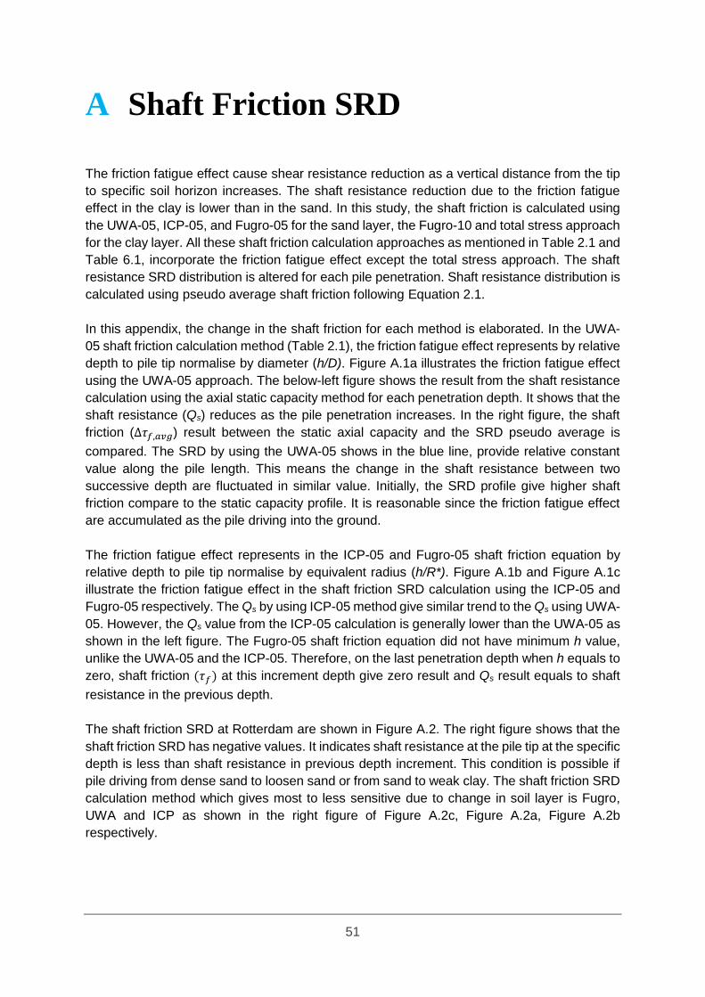
51
A Shaft Friction SRD
The friction fatigue effect cause shear resistance reduction as a vertical distance from the tip
to specific soil horizon increases. The shaft resistance reduction due to the friction fatigue
effect in the clay is lower than in the sand. In this study, the shaft friction is calculated using
the UWA-05, ICP-05, and Fugro-05 for the sand layer, the Fugro-10 and total stress approach
for the clay layer. All these shaft friction calculation approaches as mentioned in Table 2.1 and
Table 6.1, incorporate the friction fatigue effect except the total stress approach. The shaft
resistance SRD distribution is altered for each pile penetration. Shaft resistance distribution is
calculated using pseudo average shaft friction following Equation 2.1.
In this appendix, the change in the shaft friction for each method is elaborated. In the UWA-
05 shaft friction calculation method (Table 2.1), the friction fatigue effect represents by relative
depth to pile tip normalise by diameter (h/D). Figure A.1a illustrates the friction fatigue effect
using the UWA-05 approach. The below-left figure shows the result from the shaft resistance
calculation using the axial static capacity method for each penetration depth. It shows that the
shaft resistance (Qs) reduces as the pile penetration increases. In the right figure, the shaft
friction (∆𝜏𝑓,𝑎𝑣𝑔) result between the static axial capacity and the SRD pseudo average is
compared. The SRD by using the UWA-05 shows in the blue line, provide relative constant
value along the pile length. This means the change in the shaft resistance between two
successive depth are fluctuated in similar value. Initially, the SRD profile give higher shaft
friction compare to the static capacity profile. It is reasonable since the friction fatigue effect
are accumulated as the pile driving into the ground.
The friction fatigue effect represents in the ICP-05 and Fugro-05 shaft friction equation by
relative depth to pile tip normalise by equivalent radius (h/R*). Figure A.1b and Figure A.1c
illustrate the friction fatigue effect in the shaft friction SRD calculation using the ICP-05 and
Fugro-05 respectively. The Qs by using ICP-05 method give similar trend to the Qs using UWA-
05. However, the Qs value from the ICP-05 calculation is generally lower than the UWA-05 as
shown in the left figure. The Fugro-05 shaft friction equation did not have minimum h value,
unlike the UWA-05 and the ICP-05. Therefore, on the last penetration depth when h equals to
zero, shaft friction (𝜏𝑓) at this increment depth give zero result and Qs result equals to shaft
resistance in the previous depth.
The shaft friction SRD at Rotterdam are shown in Figure A.2. The right figure shows that the
shaft friction SRD has negative values. It indicates shaft resistance at the pile tip at the specific
depth is less than shaft resistance in previous depth increment. This condition is possible if
pile driving from dense sand to loosen sand or from sand to weak clay. The shaft friction SRD
calculation method which gives most to less sensitive due to change in soil layer is Fugro,
UWA and ICP as shown in the right figure of Figure A.2c, Figure A.2a, Figure A.2b
respectively.

52
(a) The UWA-05 approach
(b) The ICP-05 approach

53
(c) The Fugro-05 approach
Figure A.1 The friction fatigue effect in the shaft friction SRD at Blessington
(a) The UWA-05 in sand and the total stress approach in clay
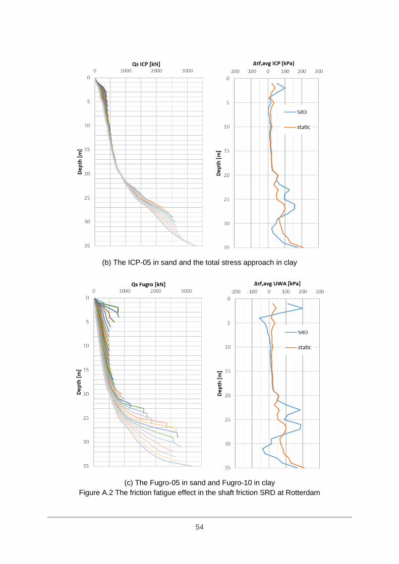
54
(b) The ICP-05 in sand and the total stress approach in clay
(c) The Fugro-05 in sand and Fugro-10 in clay
Figure A.2 The friction fatigue effect in the shaft friction SRD at Rotterdam
55
B Blessington site Result
B.1 Base Resistance-Displacement This appendix section shows the base resistance-displacement curves for piles S2-S7 at
Blessington (Figure B.1). As mentioned in Section 3.3, the base resistance-displacement
curve based on the data blow count record at the site. From the blow count/0.25m data record,
the actual pile tip displacement (wb) normalised by a number of the blow is calculated. Then,
each wb is normalised by the pile diameter. On this stage, the unit base resistance in modified
model assumes no residual base stress (qb,res) occurs in a pile. The base resistance results
from the qb - wb/D curves are implemented by using the UWA-05 approach which
accommodates partial plugging condition at pile tip.
The base resistance-displacement curves for all piles except pile S6 at Blessington which is
shown in Figure B.1 have a similar result to pile S2 which is shown in Figure 4.1. At wb/D <
0.015 in the Figure B.1, the qb - wb/D curves are increased along the pile depth. The base
resistance value from the UWA-05 approach (𝑞𝑏01,𝑈𝑊𝐴) is used as a limit at wb/D equals to
0.1. Almost all wb/D which are shown in red dot, occur at the second linear stage between
0.015 and 0.1. The wb/D are decreased as the blow counts increased at deeper pile
penetration. The wb during driving is less than failure criteria of 0.1D except for the first meter
when the pile is fully coring (IFR=1).
Figure B.1d shows the base resistance - displacement curves for pile S6. This figure shows
the actual pile tip displacement (wb) at pile S6 is smaller than other piles. As a consequence,
the pile S6 base resistance SRD value is small, in the range between 2 and 4.3 MPa. This is
unlike other piles which have the base resistance maximum average of 5.3 MPa as shown in
Table B.1. This small wb due to pile S6 has the highest blow counts record data as shown in
Figure 3.3a.
Table B.1 The base resistance – displacement average along the pile at Blessington
Pile wb/D qb [MPa] qb0,1UWA [MPa]
Min Max* Min Max Min Max
S1 0.00 0.31 0.00 5.89 2.06 8.55
S2 0.01 0.37 1.92 5.17 2.06 8.55
S3 0.01 0.37 2.00 5.19 2.06 8.55
S4 0.02 0.37 2.00 5.57 2.06 8.55
S5 0.02 0.37 2.18 5.54 2.06 8.55
S6 0.01 0.12 2.07 4.30 2.06 8.55
S7 0.02 0.21 2.11 5.45 2.06 8.19
Average 0.01 0.30 1.76 5.30 2.06 8.50 *) Maximum wb/D value in the base resistance-displacement modification is taken equal to failure criteria 0.1.
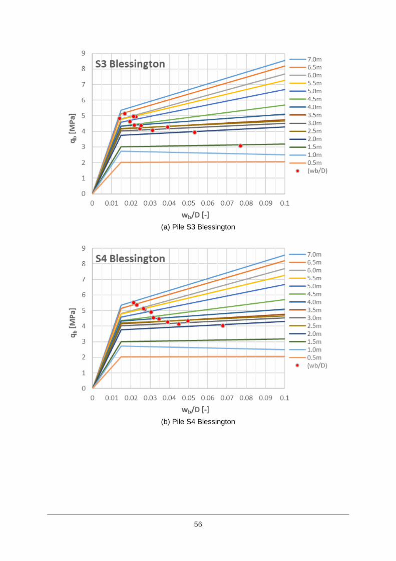
56
(a) Pile S3 Blessington
(b) Pile S4 Blessington
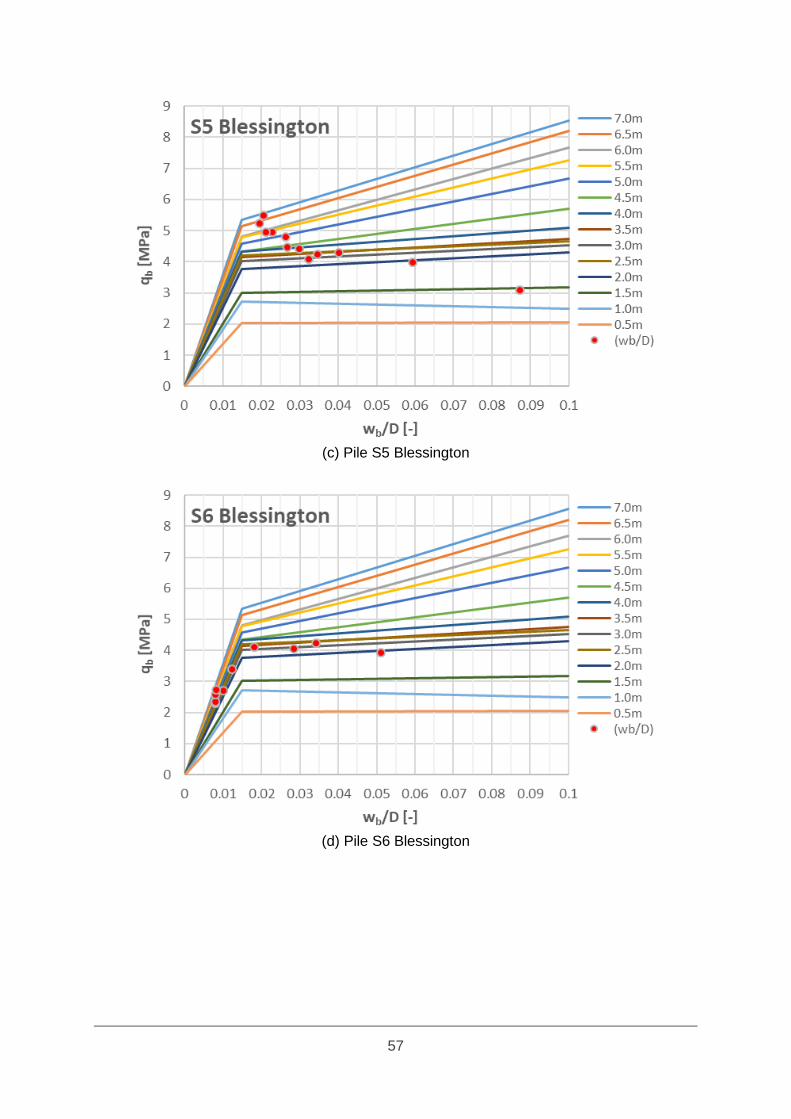
57
(c) Pile S5 Blessington
(d) Pile S6 Blessington

58
(e) Pile S7 Blessington
Figure B.1 Base resistance-displacement curves at various depth in Blessington site
B.2 Blow Count Comparison
This appendix presents the recorded and predicted blow count at Blessington piles. The
prediction result from piles S1 and S2 Blessington have been explained in Section 4.2, piles
S3-S7 are shown in Figure B.2. The estimation with a slight of underprediction and
overprediction are given when applying the unmodified model to Fugro-05 in unplugged and
ICP-05 in plugged respectively. Both unmodified model of UWA-05 and Fugro-05 in plugged
condition give poor prediction with overestimate increase along the pile depth. The unmodified
model is derived from the ICP-05 approach in unplugged condition provide under-estimate
blow counts prediction. All the unmodified models describe the soil layer along the pile.
The modified models have integrated pile ageing effects and the base-displacement model to
estimate driveability. The pile ageing applied with a time factor following Equation 3.1 is
applied to skin friction from all unmodified model along the shaft area. The unit base resistance
of UWA-05 modified further based on base-displacement as mentioned in Section 3.3. The
result of the base-displacement modification is presented in Figure B.1. The presence of
residual base stresses is ignored or assumed equals zero. The modified ICP-05 and Fugro-
05 only consider ageing effect with reducing shaft friction during driving while unit base
resistance remains the same as the unmodified model.
Generally, the prediction trend for every method is similar for every pile in Blessington except
for pile S6 and S7 as shown in Table B.2. The Coefficient of Variation (CoV) is adopted to
represent the ratio of average blow count prediction compared to the average actual blow
count record along the pile. The UWA unmodified at pile S6 give the best average CoV value
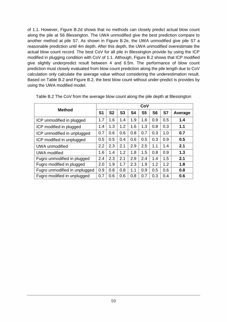
59
of 1.1. However, Figure B.2d shows that no methods can closely predict actual blow count
along the pile at S6 Blessington. The UWA unmodified give the best prediction compare to
another method at pile S7. As shown in Figure B.2e, the UWA unmodified give pile S7 a
reasonable prediction until 4m depth. After this depth, the UWA unmodified overestimate the
actual blow count record. The best CoV for all pile in Blessington provide by using the ICP
modified in plugging condition with CoV of 1.1. Although, Figure B.2 shows that ICP modified
give slightly underpredict result between 4 and 6.5m. The performance of blow count
prediction must closely evaluated from blow count prediction along the pile length due to CoV
calculation only calculate the average value without considering the underestimation result.
Based on Table B.2 and Figure B.2, the best blow count without under-predict is provides by
using the UWA modified model.
Table B.2 The CoV from the average blow count along the pile depth at Blessington
Method CoV
S1 S2 S3 S4 S5 S6 S7 Average
ICP unmodified in plugged 1.7 1.6 1.4 1.9 1.6 0.9 0.5 1.4
ICP modified in plugged 1.4 1.3 1.2 1.6 1.3 0.8 0.3 1.1
ICP unmodified in unplugged 0.7 0.6 0.6 0.8 0.7 0.3 1.0 0.7
ICP modified in unplugged 0.5 0.5 0.4 0.6 0.5 0.3 0.9 0.5
UWA unmodified 2.2 2.3 2.1 2.9 2.5 1.1 1.4 2.1
UWA modified 1.6 1.4 1.2 1.8 1.5 0.8 0.9 1.3
Fugro unmodified in plugged 2.4 2.3 2.1 2.9 2.4 1.4 1.5 2.1
Fugro modified in plugged 2.0 1.9 1.7 2.3 1.9 1.2 1.2 1.8
Fugro unmodified in unplugged 0.9 0.8 0.8 1.1 0.9 0.5 0.6 0.8
Fugro modified in unplugged 0.7 0.6 0.6 0.8 0.7 0.3 0.4 0.6

60
(a) Pile S3 Blessington
(b) Pile S4 Blessington
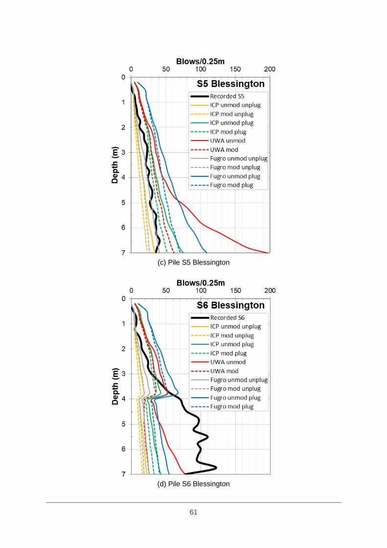
61
(c) Pile S5 Blessington
(d) Pile S6 Blessington

62
(e) Pile S7 Blessington
Figure B.2 Recorded and predicted blow count comparison at Blessington site
B.3 Residual Base Stresses
The base resistance by using the UWA-05 are modified further to account for the residual
base stresses. The residual base stresses occur after each hammer blow during pile
installation. In this modification, the model has integrated not only the base resistance-
displacement but also the residual base stresses. The residual base stress is cooperated with
adding {1,2,5,8,10}% of the cone tip resistance (qc) to the unit base stress as mentioned in
Section 3.4. The additional base residual must less than the negative shaft resistance
available at the specific pile depth penetration. The model takes the time factor due to the
ageing effect and a tension factor as a recommended by the UWA-05. The time factor and
tension capacity are used when calculating the negative shaft resistance. The SRD profile for
the UWA-05 modified including base resistance residual are derived after ensuring that base
resistance load less than the negative shaft resistance.
Figure B.3 shows the recorded and modified additional base residual stresses at Blessington.
This figure shows that residual base stresses developed along the pile length with the highest
value of 4 MPa at the pile base. There is no modified additional base residual stress that
matches entirely along the pile length. The close base residual stresses model is given by
using 8% qc between 3 and 5m depth and 19% qc at the final depth.
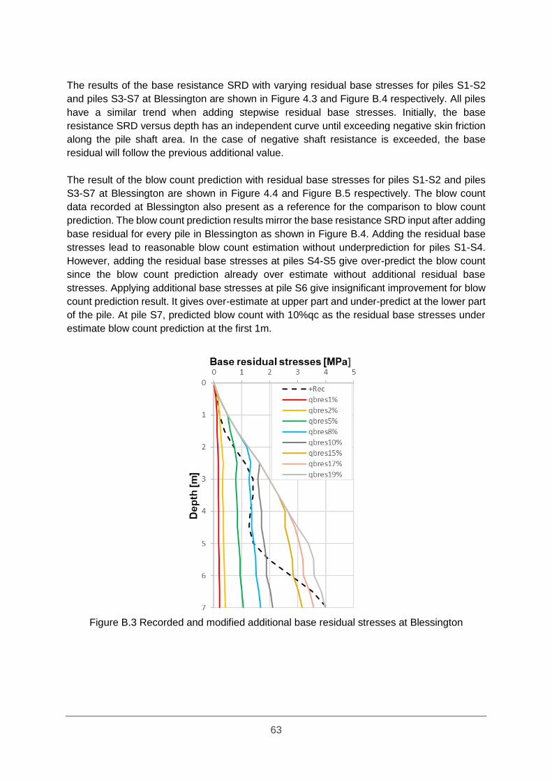
63
The results of the base resistance SRD with varying residual base stresses for piles S1-S2
and piles S3-S7 at Blessington are shown in Figure 4.3 and Figure B.4 respectively. All piles
have a similar trend when adding stepwise residual base stresses. Initially, the base
resistance SRD versus depth has an independent curve until exceeding negative skin friction
along the pile shaft area. In the case of negative shaft resistance is exceeded, the base
residual will follow the previous additional value.
The result of the blow count prediction with residual base stresses for piles S1-S2 and piles
S3-S7 at Blessington are shown in Figure 4.4 and Figure B.5 respectively. The blow count
data recorded at Blessington also present as a reference for the comparison to blow count
prediction. The blow count prediction results mirror the base resistance SRD input after adding
base residual for every pile in Blessington as shown in Figure B.4. Adding the residual base
stresses lead to reasonable blow count estimation without underprediction for piles S1-S4.
However, adding the residual base stresses at piles S4-S5 give over-predict the blow count
since the blow count prediction already over estimate without additional residual base
stresses. Applying additional base stresses at pile S6 give insignificant improvement for blow
count prediction result. It gives over-estimate at upper part and under-predict at the lower part
of the pile. At pile S7, predicted blow count with 10%qc as the residual base stresses under
estimate blow count prediction at the first 1m.
Figure B.3 Recorded and modified additional base residual stresses at Blessington

64
(a) Pile S3 Blessington (b) Pile S4 Blessington
(c) Pile S5 Blessington (d) Pile S6 Blessington
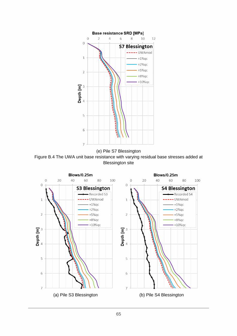
65
(e) Pile S7 Blessington
Figure B.4 The UWA unit base resistance with varying residual base stresses added at
Blessington site
(a) Pile S3 Blessington (b) Pile S4 Blessington
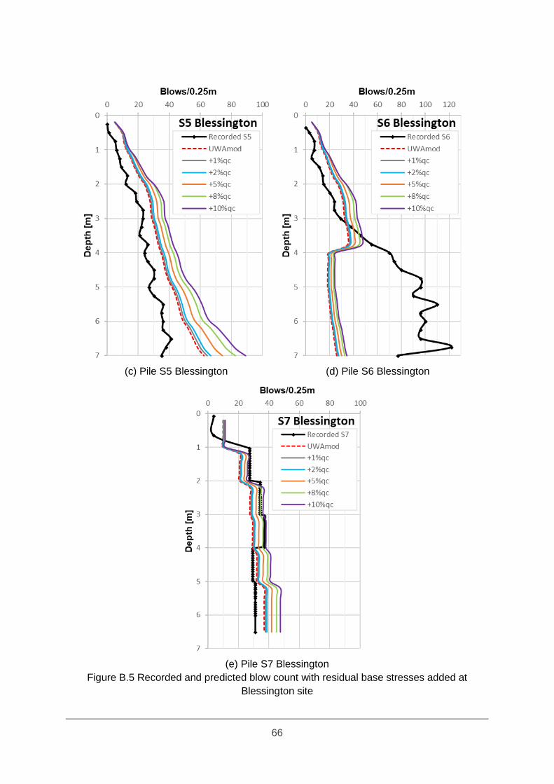
66
(c) Pile S5 Blessington (d) Pile S6 Blessington
(e) Pile S7 Blessington
Figure B.5 Recorded and predicted blow count with residual base stresses added at
Blessington site
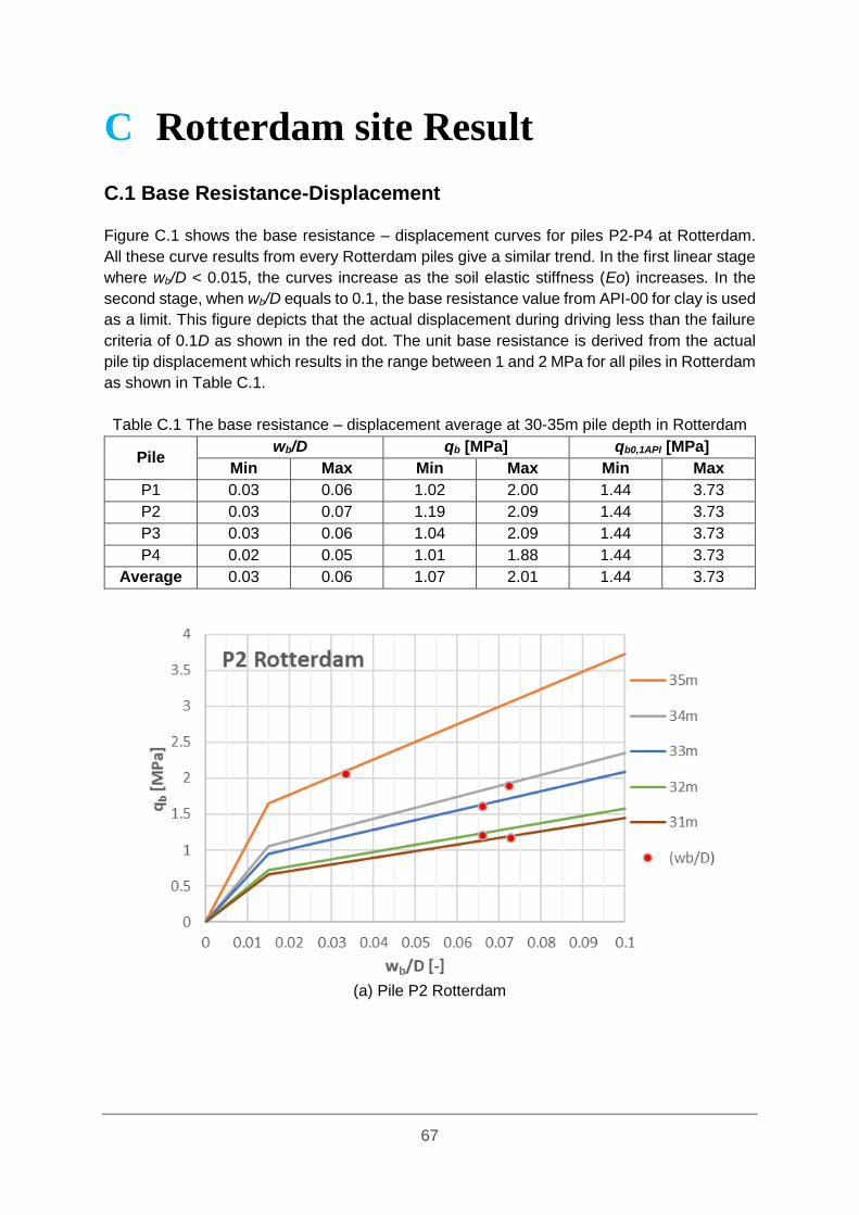
67
C Rotterdam site Result
C.1 Base Resistance-Displacement Figure C.1 shows the base resistance – displacement curves for piles P2-P4 at Rotterdam.
All these curve results from every Rotterdam piles give a similar trend. In the first linear stage
where wb/D < 0.015, the curves increase as the soil elastic stiffness (Eo) increases. In the
second stage, when wb/D equals to 0.1, the base resistance value from API-00 for clay is used
as a limit. This figure depicts that the actual displacement during driving less than the failure
criteria of 0.1D as shown in the red dot. The unit base resistance is derived from the actual
pile tip displacement which results in the range between 1 and 2 MPa for all piles in Rotterdam
as shown in Table C.1.
Table C.1 The base resistance – displacement average at 30-35m pile depth in Rotterdam
Pile wb/D qb [MPa] qb0,1API [MPa]
Min Max Min Max Min Max
P1 0.03 0.06 1.02 2.00 1.44 3.73
P2 0.03 0.07 1.19 2.09 1.44 3.73
P3 0.03 0.06 1.04 2.09 1.44 3.73
P4 0.02 0.05 1.01 1.88 1.44 3.73
Average 0.03 0.06 1.07 2.01 1.44 3.73
(a) Pile P2 Rotterdam

68
(b) Pile P3 Rotterdam
(c) Pile P4 Rotterdam
Figure C.1 Base resistance-displacement curves at various driving depth in Rotterdam site
C.2 Blow Count Comparison Figure C.2 shows the recorded and the predicted blow count for piles S2-S4 at Rotterdam. All
the results are alike for all piles in the Rotterdam. These are results by using the combination
of CPT-based approaches for soil profile in sand and clay. In the upper clay layer, at 4m until
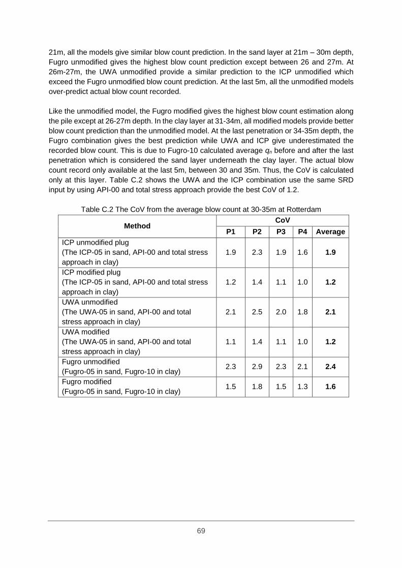
69
21m, all the models give similar blow count prediction. In the sand layer at 21m – 30m depth,
Fugro unmodified gives the highest blow count prediction except between 26 and 27m. At
26m-27m, the UWA unmodified provide a similar prediction to the ICP unmodified which
exceed the Fugro unmodified blow count prediction. At the last 5m, all the unmodified models
over-predict actual blow count recorded.
Like the unmodified model, the Fugro modified gives the highest blow count estimation along
the pile except at 26-27m depth. In the clay layer at 31-34m, all modified models provide better
blow count prediction than the unmodified model. At the last penetration or 34-35m depth, the
Fugro combination gives the best prediction while UWA and ICP give underestimated the
recorded blow count. This is due to Fugro-10 calculated average qn before and after the last
penetration which is considered the sand layer underneath the clay layer. The actual blow
count record only available at the last 5m, between 30 and 35m. Thus, the CoV is calculated
only at this layer. Table C.2 shows the UWA and the ICP combination use the same SRD
input by using API-00 and total stress approach provide the best CoV of 1.2.
Table C.2 The CoV from the average blow count at 30-35m at Rotterdam
Method CoV
P1 P2 P3 P4 Average
ICP unmodified plug
(The ICP-05 in sand, API-00 and total stress
approach in clay)
1.9 2.3 1.9 1.6 1.9
ICP modified plug
(The ICP-05 in sand, API-00 and total stress
approach in clay)
1.2 1.4 1.1 1.0 1.2
UWA unmodified
(The UWA-05 in sand, API-00 and total
stress approach in clay)
2.1 2.5 2.0 1.8 2.1
UWA modified
(The UWA-05 in sand, API-00 and total
stress approach in clay)
1.1 1.4 1.1 1.0 1.2
Fugro unmodified
(Fugro-05 in sand, Fugro-10 in clay) 2.3 2.9 2.3 2.1 2.4
Fugro modified
(Fugro-05 in sand, Fugro-10 in clay) 1.5 1.8 1.5 1.3 1.6
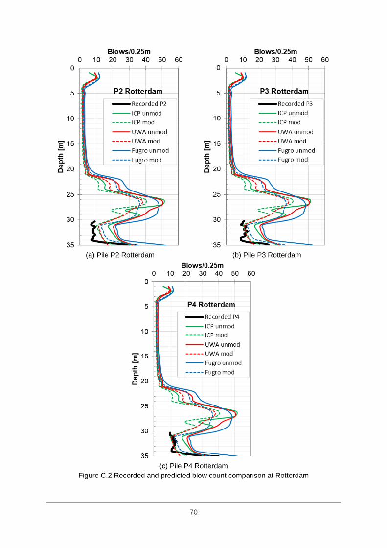
70
(a) Pile P2 Rotterdam
(b) Pile P3 Rotterdam
(c) Pile P4 Rotterdam
Figure C.2 Recorded and predicted blow count comparison at Rotterdam

71
C.3 Residual Base Stresses
At Rotterdam, the base resistance for combine UWA is modified further not only with base
resistance-displacement but also by using the residual base stresses which occur after each
hammer blow. The combined UWA method is derived by using a combination of the UWA-05
in sand, the total stress approach in clay for skin friction calculation and the API-00 in clay for
base resistance calculation. The base residual stress is calculated by sensitivity analysis of
stepwise {1%, 2%, 5%, 8%, 10%} of cone tip resistance (qc) as mentioned in Section 3.4. The
base resistance stress is added to the base resistance must less than available negative skin
friction at that specific depth.
The results of the base resistance SRD with varying residual base stresses for pile P1 and
piles P2-P3 at Rotterdam are shown in Figure 6.5a and Figure C.3 respectively. All piles at
Rotterdam have a similar trend when adding stepwise residual base stresses. The clay layer
between 4 and 21m depth have small qc which lead unnoticeable addition to the base
resistance SRD. A distinct change in the base resistance SRD result are observed at the sand
layer between 22 and 30m.
The result of the blow count prediction with residual base stresses for pile P1 and piles P2-P4
at Rotterdam are shown in Figure 6.5b and Figure C.4 respectively. There is insignificant
change in the clay layer causing the blow count result in almost the same prediction. A
noticeable alteration in the blow count results is presented in the sand layer at 21m until 30m.
At 27m depth, the blow count increases 1 blow/0.25m when the additional base residual to
the base resistance SRD increases from 1% qc to 2% qc. This increase trend is applied for all
piles in the Rotterdam.

72
(a) Pile P2 Rotterdam (b) Pile P3 Rotterdam
(c) Pile P4 Rotterdam
Figure C.3 The UWA unit base resistance with varying residual base stresses added at
Rotterdam site
73
(a) Pile P2 Rotterdam (b) Pile P3 Rotterdam
(c) Pile P4 Rotterdam
Figure C.4 Recorded and predicted blow count with residual base stresses added at
Rotterdam site


![Titel · Web viewA simple cognitive task using the nine numerical characters modified from Conners’ Continuous Performance Test (CPT) [8] was adopted to numerically evaluate sustained](https://static.documents.pub/doc/80x56/5e6e6db5e3c508445a564f98/web-view-a-simple-cognitive-task-using-the-nine-numerical-characters-modified-from.jpg)


