Crack propagation in dynamics by embedded strong ...

HAL Id: hal-01996636https://hal.utc.fr/hal-01996636

Submitted on 5 Feb 2019

HAL is a multi-disciplinary open accessarchive for the deposit and dissemination of sci-entific research documents, whether they are pub-lished or not. The documents may come fromteaching and research institutions in France orabroad, or from public or private research centers.

L’archive ouverte pluridisciplinaire HAL, estdestinée au dépôt et à la diffusion de documentsscientifiques de niveau recherche, publiés ou non,émanant des établissements d’enseignement et derecherche français ou étrangers, des laboratoirespublics ou privés.

Crack propagation in dynamics by embedded strongdiscontinuity approach: Enhanced solid versus discrete

lattice modelMijo Nikolić, Xuan Do, Adnan Ibrahimbegovic, Željana Nikolić

To cite this version:Mijo Nikolić, Xuan Do, Adnan Ibrahimbegovic, Željana Nikolić. Crack propagation in dynam-ics by embedded strong discontinuity approach: Enhanced solid versus discrete lattice model.Computer Methods in Applied Mechanics and Engineering, Elsevier, 2018, 340, pp.480-499.10.1016/j.cma.2018.06.012. hal-01996636

https://hal.utc.fr/hal-01996636

https://hal.archives-ouvertes.fr

Available online at www.sciencedirect.com

ScienceDirect

Comput. Methods Appl. Mech. Engrg. 340 (2018) 480–499www.elsevier.com/locate/cma

Crack propagation in dynamics by embedded strong discontinuityapproach: Enhanced solid versus discrete lattice model

Mijo Nikolicb, Xuan Nam Doa, Adnan Ibrahimbegovica,∗, Željana Nikolicb

a Université de Technologie de Compiègne/Sorbonne Universités, Laboratoire Roberval de Mécanique, Centre de Recherche Royallieu, 60200Compiègne, France

b University of Split, Faculty of Civil Engineering, Architecture and Geodesy, 21000 Split, Croatia

Received 6 December 2017; received in revised form 5 April 2018; accepted 7 June 2018Available online 20 June 2018

Abstract

In this work we propose and compare the two models for crack propagation in dynamics. Both models are based on embeddedstrong discontinuities for localized cohesive type crack description and both provide the advantage to not to require trackingalgorithms. The first one is based on discrete lattice approach, where the domain is discretized with Voronoi cells held togetherprior to crack occurrence by cohesive links represented in terms of Timoshenko beams. The second one is based on constantstrain triangular solid element. In both models, propagation of cracks activates enhancements in the displacement field leadingto embedded strong discontinuities. The latter remain localized inside the element, regulated by the localized traction separationbehavior defined through exponential softening law. Thus, the both models provide the result that remain mesh-independent,with fracture energy as the model parameter. We show that implementation in dynamics framework can be obtained by addinginertial effects without modifying the existing quasi-statics models. In order to provide reliable results, classical implicit Newmarkalgorithm can be used for time integration. The two presented models are subjected to dynamic crack propagation benchmarks,where detailed analysis on strain, kinetic, plastic free and dissipated energy during simulation is verified by comparison to theamount of total work which is introduced into the system. The main strength of the proposed approach is that cracks initiation,propagation, their coalescence, merging and branching are automatically obtained without any tracking algorithms. In addition,since the discontinuities remain localized inside elements, accurate results can be obtained even with coarser grids, leading toefficient methodology capable of capturing complex crack patterns in dynamics.

c⃝ 2018 Elsevier B.V. All rights reserved.

Keywords: Dynamic crack propagation; Embedded strong discontinuities; Localized failure; Plastic free energy; Damage free energy; Kineticenergy; Strain energy

∗ Corresponding author.E-mail address: [email protected] (A. Ibrahimbegovic).

https://doi.org/10.1016/j.cma.2018.06.0120045-7825/ c⃝ 2018 Elsevier B.V. All rights reserved.

http://crossmark.crossref.org/dialog/?doi=10.1016/j.cma.2018.06.012&domain=pdf

http://www.elsevier.com/locate/cma

https://doi.org/10.1016/j.cma.2018.06.012

http://www.elsevier.com/locate/cma

mailto:[email protected]

https://doi.org/10.1016/j.cma.2018.06.012

M. Nikolic et al. / Comput. Methods Appl. Mech. Engrg. 340 (2018) 480–499 481

1. Introduction

The description of dynamic crack propagation remains challenging task due to the presence of complex phenomenapertinent to cracks initiation, propagation and growth, branching, multiple cracks interaction, their coalescence andmerging. These phenomena are also under the strong influence of the size of the fracture process zone (FPZ), i.e. thezone around the crack where nonlinear and dissipative mechanisms occur. Numerical methods are often the only wayto find the solution for such problem, with the main challenge to make it reliable. Since the standard finite elementprocedure shows strong dependence on mesh when simulating cracks [1], many enhanced and extended finite elementmethods based on inserting discontinuity lines and enriching the displacement fields, have been developed. Dependingon the type of material and the size of the FPZ, one can choose the enrichments for the method either based on thetheory of linear elastic fracture mechanics (LEFM) or cohesive zone formulation. LEFM can be used in the case whenFPZ around the crack (and the crack tip) is small compared to the size of the crack or specimen, and when the bulk isisotropic and linear elastic. For instance, extended finite element method (X-FEM) with crack tip asymptotic fields anddiscontinuous enrichment for displacement jump across the crack line can be found in [2–4]. On the other hand, whenLEFM is not applicable and when FPZ influences the behavior of the material, cohesive type formulation of fracturecan be used. Cohesive approach is described as a gradual separation of crack surfaces across the crack tip or cohesivezone which is resisted by cohesive tractions when material elements are pulled away. Namely, once the critical valueof traction is reached, softening in material is triggered with decreasing traction and increasing crack opening. Thisrepresents the constitutive model for crack opening and input for our simulations. Enhanced methods which allow forarbitrary cohesive crack growth are cohesive X-FEM [5–7] and embedded strong discontinuity finite element method(ED-FEM) [8–10]. They can both deal with cracks in a mesh independent way due to their enrichments. Trackingalgorithms, which can be quite computationally costly, are often used with these methods, especially to solve thecomplex crack phenomena in dynamics, such as branching. Recently, phase field models [11,12] have been used tosuccessfully represent complex brittle crack behavior in dynamics, by smearing and smoothening the boundary of thecrack over a small region. They can be used to avoid tracking algorithms, but apparently very fine meshes usuallywith adaptive refinement are needed to resolve steep displacement fields.

In this work we propose the two models for dynamic crack growth based on localized cohesive crack representation,which will also surpass the need for crack tracking algorithms, and that moreover can be equally used for fine andcoarse mesh. Both models are based on embedded strong discontinuity approach (ED-FEM), which is a discretecrack description where displacement fields are enhanced with additional kinematics to provide displacement jumps[8]. The main difference with respect to X-FEM (see [13]), where discontinuity is considered globally throughadditional nodal unknowns, is that additional degrees of freedom and corresponding enrichment functions relatedto crack opening are kept at the element level. One can solve the corresponding equations locally, which allows forthe straightforward implementation within standard computer code architecture. Any ED-FEM formulation provideslocalized interpretation of cracks leading to mesh-independent post-peak softening response, which is defined throughcohesive traction separation law. Mesh independency is considered here in the context of fracture energy, which weuse here as the input parameter for our cohesive softening behavior. Namely, it has been observed that softening curvedepends on the size of the FPZ and dissipative mechanisms in the zone. The main benefit of present formulation isthat it acts as a natural localization limiter for the FPZ and one does not need to implement the characteristic lengthparameter to stabilize its size and correspondingly the post-peak softening behavior [1,14].

The first model that we propose herein relies on discrete lattice element approach with embedded strongdiscontinuities for quasi-static crack propagation described in [14]. In the present work we extend such quasi-staticformulation into dynamic framework. The second model is based on enhanced triangular constant strain element wherestrain localization band collapses into a surface leading to embedded strong discontinuity, or jump in displacementfield. The latter approach is described in [15] for quasi static case with further development to show how to extendit to dynamic framework in [16], and its resulting benefits for quasi-static test with slow loading rate in reducing thetotal number of iterations. Here we seek to extend these two models and to provide their validation on well knowndynamic benchmarks. The difference in the two models is that post-peak softening behavior related to discontinuity isgoverned by plasticity framework in discrete lattice model, while damage framework is chosen in enhanced triangularmodel. This is applicable in quasi brittle or plastic materials with pronounced FPZ where diffuse micro-cracks orplastic dissipation around the crack and crack tip influence the failure mechanisms. Although these two modelsare different and are initially developed for different purposes (the presented discrete lattice model is developed forfailure in heterogeneous quasi brittle materials such as rocks and concrete, while enhanced solid triangular element is

482 M. Nikolic et al. / Comput. Methods Appl. Mech. Engrg. 340 (2018) 480–499

developed for failure in solids), they have similarities and common strengths allowing us to summarize the features ofthe approach based on embedded strong discontinuity crack description:

• embedded strong discontinuity can represent localized and arbitrary crack growth with cohesive approach inwhich discontinuous enrichment is coupled with softening traction separation law

• due to local element-wise crack description, tracking algorithms are not needed (although some ED-FEMbased models use it) since complex stress states and material structure can automatically drive correct crackpropagation

• multiple cracks with their interaction, coalescence or branching can easily be obtained automatically withoutadditional complexities and interventions

• embedded strong discontinuity formulation guarantees mesh independence in terms of fracture energies in post-peak softening regime, which is also confirmed in this work with extensive simulations with different meshsizes. Moreover, accurate complex crack patterns and failure mechanisms can be obtained with fairly coarsegrids leading to high computational efficiency

• complete simulation is performed on initial mesh, which does not need to be updated during the crack evolution• brittle and ductile cracks with pronounced FPZ can be captured by choosing appropriate level of fracture energy.

They can also be triggered with mode I leading to tensile cracks and mode II resulting in shear bands.

The main reason for mesh-independent representation in ED-FEM approach is that discontinuity, or displacementjump, always remains localized inside the element and behaves as a localization limiter that enhances theclassical continuum mechanics theoretical formulation. The numerical implementation of the discontinuity requires amodification of the standard finite element procedure, which is similar to the method of incompatible modes [17].

The appealing fact in the strong discontinuity concept is also that dynamics framework can be built up withoutextensively changing existing codes developed for quasi-static cases. In particular, inertial terms based on globalmass matrix do not modify the local element-wise problem of discontinuity. The global dynamics equation of motioncan then be integrated in time with existing time integration schemes. Here, we use the classical Newmark implicitalgorithm for global time integration in order to provide more reliable solution. The local time integration for plasticityand damage evolution of discontinuities are also performed implicitly to keep the same solution reliability.

The paper is organized as follows. Section 2 presents the discrete lattice model with embedded strong discon-tinuities developed in dynamics framework. Section 3 gives the description of enhanced triangular solid modelwith embedded strong discontinuities in dynamic framework. Section 4 provides the numerical simulations of wellknown dynamic benchmarks for crack propagation performed with both models. Besides crack patterns, we also givequantitative values for energy dissipation and plastic/damage free energy during the crack evolution, together withstrain and kinetic energy. All components of energy are verified by comparison to the total amount of input workwhich is introduced into the system. Conclusion is given in Section 5.

2. Discrete lattice model with embedded strong discontinuities

The proposed discrete lattice model has been developed for quasi-static propagation of cracks in heterogeneousmaterials and already applied in progressive failure simulations of rocks [18,19], concrete [20] and saturated porousmedium [21,22]. It relies on representing the cohesive links by spatial beam models, as a class of discrete latticemodels where geometry is built using Delaunay triangulation. Here, the Delaunay edges in triangulation can beconsidered as lattice elements representing cohesive links between the Voronoi cells, each filled-in with a singlephase of material (Fig. 1.a). Such structure allows for cracks representation with a progressive failure of adjacentcohesive links (Fig. 1.c). In this approach we simulate lattice elements with enhanced 2D Timoshenko beams in orderto provide the complete set of 2D failure modes, with mode I as tensile crack opening and mode II as shear sliding.Each failure mode activates an embedded strong discontinuity in corresponding direction. The geometric propertiessuch as the beams cross section can easily be extracted from the area (line in 2D) between two neighboring Voronoicells (Fig. 1.b). Thus, the global stiffness of the mesh is controlled by the size of the cross sections of Timoshenkobeams.

Generally, discrete lattice models have been extensively used to successfully represent complex failure mechanismsoccurring in heterogeneous materials, such as concrete or rocks [23–26]. They have also been applied in multiphysicsfailure applications [27,28], thermal conductivity [29], vibration analysis [30,31], dynamic crack propagation [32,33]


Fig. 1. (a) Structure of discrete lattice model with Voronoi cells as units of heterogeneous material and cohesive links between them (b) neighboringVoronoi cells—h is extracted from Voronoi diagram and represents the height of the beam cross section. By coarsening or refining mesh, hcorrespondingly increases or decreases which keeps the global stiffness of the specimen steady (c) failure of adjacent cohesive links.

and impact applications [34,35]. However, none of these models is comparable to the present model, which providesthe failure mechanisms in mode I and mode II in terms of embedded discontinuities in Timoshenko lattice beamelements.

In the proposed model, the discrete lattice structure allows to find the solution for dynamic crack propagation,interaction of multiple cracks and fracture process zone without any additional global degrees of freedom oralgorithms for crack tracking. Moreover, the embedded discontinuities allow to represent failure and softening withoutdependence on mesh.

Next we give the formulation for 2D Timoshenko beam element enhanced with embedded strong discontinuity,which is capable to provide failure mechanisms and corresponding displacement jump inside the element (Fig. 1.c).The occurrence of jump in the displacement field is followed by softening plasticity behavior. One can trigger jumpin normal displacement for mode I and transverse displacement for mode II.

2.1. Enhanced kinematics of 2D Timoshenko beam element

One can start from standard kinematics of a geometrically linear Timoshenko beam finite element of length le andcross section A = h · 1 in order to obtain the strain measures ϵ

ϵ(x) =

⎡⎢⎢⎢⎢⎣ϵ(x) =

dudx

γ (x) =dvdx

− θ

κ(x) =dθdx

⎤⎥⎥⎥⎥⎦ (1)

where u = [u v θ]T is the generalized displacement vector with longitudinal displacement, transverse displacementand rotation as shown in Fig. 2 and ϵ =

[ϵ γ κ

]T is a corresponding strain vector.In order to represent the mode I as axial failure and mode II failure as shear failure, we introduce discontinuities in

the generalized displacement field of the 2D Timoshenko beam. This is achieved with Heaviside function Hxc definedby Hxc (x) = 0 for x ≤ xc and Hxc (x) = 1 and vector α = [αu αv 0]T which represents the vector of displacementjumps at the point of discontinuity xc placed in the middle of the beam. The position of discontinuity correspondsto intersection of the neighboring Voronoi cells (Fig. 1.c). The embedded strong discontinuity inside element willallow to provide mesh independent response in terms of energy for softening law. More precisely, fracture energyas input parameter will remain independent on mesh. We can write the displacement field as the sum of continuousdisplacement and a displacement jump as

u(x) = u(x) + αHxc =

⎡⎣u(x)v(x)θ (x)

⎤⎦+

⎡⎣αu

αv0

⎤⎦ Hxc . (2)


Fig. 2. Timoshenko beam with standard degrees of freedom and additional ones related to jumps in the displacement fields. M(x) and G(x) are thediscontinuity related additional enrichment functions.

Thus, Eq. (2) can be rewritten by adding and subtracting a regular differentiable function from Heaviside function(see [20] for more details) and the resulting finite element interpolations for displacement field can be recast as

u(x) = N1(x)u1 + N2(x)u2 + α (Hxc − N2(x)) M(x)

(3)

where regular part of Timoshenko beam displacements is interpolated with shape functions as linear polynomials,N1(x) = 1 −

xle

, N2(x) =xle

. An additional discontinuity-related unknown is accompanied by enrichment function fordisplacement field denoted as M

M(x) =

−xle

; x ∈ [0, xc⟩

1 −xle

; x ∈ ⟨xc, le].(4)

The function M(x) (see Fig. 2) is an element enrichment function, containing element unit jump function, whichcharacterizes the embedded discontinuity approach where the contribution of the discontinuity will cancel at elementnodes leaving only standard nodal unknowns. Moreover, additional discontinuity degrees of freedom α can be keptinside the element, which are solved for at the element level by computation that are independent on the global finiteelement procedure. We can write the enhanced total displacement field in a matrix form as

u = Nua + Mα (5)

with N as 3 × 6 matrix containing element shape functions N1(x) and N2(x), and M is 3 × 3 matrix containingdiscontinuity interpolation functions M positioned at the first two diagonal entries related to translational degrees offreedom, leaving rotation interpolation intact.

Interpolation of enhanced strain field requires the derivatives of shape functions B1(x) = −1le

, B2(x) =1le

and thederivative G of enrichment M , leading to

G(x) = G(x) + δxc , G(x) = −1le. (6)

The function G is split into regular part G and singular part in terms of δxc . The expression above reduces toG(x) = −B2(x). The interpolated enhanced strain field can be obtained with

ϵ = Bua + Gα + αδxc (7)

where B is 3 × 6 beam strain–displacement matrix corresponding to Eq. (1) and G is the 3 × 3 matrix of derivativesof discontinuity enriched function G at the entries related to translational degrees of freedom.


2.2. Variational equation

The virtual strain field can be constructed in the same way as real enhanced strain field

δϵ = Bδua + Gvδα + δαδxc (8)

where δua and δα represent virtual displacement field and virtual displacement jump. We can build the virtual workequation G int,(e)

−Gext,(e)= 0, where internal work is defined as G int,(e)

=∫ le

0 (δϵ)T σdx . The finite element assemblyprocedure with enhanced elements produces the two groups of equations

Anele=1

(fint,(e)

− fext)= 0

h(e)=

∫ le

0GT

σdx + t, ∀e ∈ [1, nel].(9)

The first of these is a set of global equations where f int,(e)=∫ le

0 BT σdx . The second equation with condition h(e)= 0

needs to be enforced in each element where discontinuity is activated, which leads to definition of the traction vectorat discontinuity

t = −

∫ le

0Gσdx . (10)

Note that assembly operator in the first equation in (9) considers all elements, while the second equation remainslimited to a particular element due to character of interpolation function for discontinuity which takes zero values atthe element boundary.

In order to solve the nonlinear problem addressed in Eq. (9), the consistent linearization (e.g. see [1]) of bothequations has to be performed. The standard Newton incremental-iterative procedure is used to provide new iterativevalues of nodal displacements

Anele=1

[Ke,(i)

n+1∆u(i)n+1 + Fe,(i)

n+1∆α(i)n+1

]= Anel

e=1

[fext,en+1 − fint,e,(i)

n+1

]he,(i)

n+1 +

(Fe,(i)v,n+1 + K(i)

d,n+1

)∆u(i)

n+1 +

(He,(i)

n+1 + K(i)α,n+1

)∆α

(i)n+1 = 0

(11)

where the explicit form of matrices is

Ke,(i)n+1 =

∫ le

0BT C(i)

n+1Bdx, Fe,(i)n+1 =

∫ le

0BT C(i)

n+1Gdx

Fe,(i)v,n+1 =

∫ le

0GT C(i)

n+1Bdx, He,(i)n+1 =

∫ le

0GT C(i)

n+1Gdx(12)

and C(i)n+1 = diag(E A,G A, E I ) is the tangent stiffness for 3D Timoshenko beam. Similarly, K(i)

d,n+1 and K(i)α,n+1 are

the consistent tangent stiffness for discontinuity

∆t(i)n+1 = K(i)

d,n+1∆u(i)n+1 + K(i)

α,n+1∆α(i)n+1. (13)

Enforcement of the local equation in (9) allows us to exploit the static condensation of the additional degrees offreedom (e.g. [1]). This leads to the reduced size of stiffness matrix corresponding to global unknowns only, which iscalculated as follows:

Ke,(i)n+1 = Ke,(i)

n+1 − Fe,(i),Tn+1 (He,(i)

n+1 + K (i)α,n+1)−1(Fe,(i)

v,n+1 + K (i)d,n+1). (14)

A reduced stiffness matrix contributes to finite element assembly procedure to provide global set of linearizedequilibrium equations. Computed incremental displacements ∆u(i)

n+1 are used to perform corresponding displacementvector update

Anele=1Ke

n+1∆u(i)n+1 = Anel

e=1


n+1

]H⇒ u(i+1)

n+1 = u(i)n+1 + ∆u(i)

n+1.(15)


2.3. Extension to dynamics

Since embedded discontinuity contribution is kept at the element level with internal force vector fint,e,(i)n+1 contained

inside an element, one can easily extend the proposed approach to the dynamics framework by applying thed’Alembert principle to the system of equations written above. By applying the standard finite element interpolationsand assembly procedure, classical global system of equations of motion Man+1+fint

n+1 = fextn+1 is obtained. Global mass

matrix M = Anele=1Me is assembled from element mass matrices Me

=∫ le

0 NTρANdx , where ρ represents materialdensity and A beam cross section. Vector an+1 contains nodal accelerations.

One can apply the classical implicit Newmark scheme to solve the corresponding dynamics equation of motion.The displacement and velocity updates can be expressed in terms of Newmark’s β and γ parameters as

un+1 = un + ∆tvn + (∆t)2[

(12

− β)an + βan+1

]vn+1 = vn + ∆t

[(1 − γ )an + γ an+1

] (16)

where ∆t is increment in time. In order to solve nonlinear equations of motion, we can first combine Eqs. (16) toobtain an+1

an+1 = −

12 − β

βan −

vn

β∆t+

1(∆t)2β

(un+1 − un). (17)

The linearization procedure on the result in (17) will provide the possible iterative improvement and updatesun+1 = u(i)

n+1 + ∆u(i)n+1. The insertion of linearized equation (17) into equations of motion will produce the following

system of equations which can be solved by Newton procedure:

Anele=1

(1

(∆t)2βMe

+ Ken+1

)∆u(i)

n+1 = Anele=1


n+1 − Mea(i)n+1

]H⇒ u(i+1)

n+1 = u(i)n+1 + ∆u(i)

n+1.

(18)

It is important to note that embedded discontinuity is confined in internal force vector and that statically condensedstiffness matrix still remains the same like in quasi-static case. Moreover, the corresponding extension for dynamiccrack propagation can be performed just by adding inertial terms on top of existing formulation for quasi-static case.Here, we use Newmark’s parameters β = 1/4 and γ = 1/2 and Newton’s algorithm with line search to obtain thecorresponding displacement update and solution of nonlinear system. Note that we did not have to use any additionaldamping matrix or other similar contribution.

2.4. Plastic softening

Internal force vector in (9) in a beam lattice contains stress resultants σ =[N V M

]T , where axial and shearare computed with softening plasticity as a result of occurrence of failure modes I and II activated upon reachingfailure threshold. The response to rotation is kept linear elastic. The evolution of softening plasticity variables isgoverned by singular part of deformation field at the position of discontinuity, while stress field remains smooth [8].The computation of vector σ can be split into two scalar equations, where each failure mode appears separately. Inorder to simplify the following presentation, we will write the scalar equations, which are valid for computation of bothfailure modes and corresponding stress resultants in axial and transverse directions. Here we start with a Helmholtzfree energy potential for softening plasticity

Ψ (σ, q) =12σϵe Ψel

+Ξ (ξ )Ψ pl

; Ξ (ξ ) = −qξ (19)

where ξ represents internal softening variable, ϵe is elastic strain and q is a stress-like softening variable defined withexponential softening constitutive law for discontinuity

q = σu

(1 − exp

(−ξ

σu

G f

))(20)


G f is the corresponding value of fracture energy representing input parameter, σu is the failure threshold for mode I.We use τu as a threshold for mode II. We can write the failure detection function for softening as

Φ (t, q) = t − (σu − q) ≤ 0 (21)

where t is a traction acting at the discontinuity computed from (10).The evolution equations for discontinuity can be written similarly to standard plasticity with the main difference

that the plastic deformation in softening remains localized at the particular point (represented by the Dirac function)

α = λ∂Φ

∂σ= λsign(σ )

ξ = λ∂Φ

∂q= λ

(22)

where λ is the plastic multiplier associated with the softening behavior and α is equivalent to the accumulated plasticstrain at the discontinuity. The plastic dissipation in softening plasticity can be obtained with the second law ofthermodynamics and written in a distributional sense. Its local form is given as (see also [8])

DP = σ ϵ −ddt

Ψ (σ, q) = [sign(σ ) + q(ξ )] σu

ξ . (23)

The total energy balance involving first and second laws of thermodynamics in any finite element elastoplastic modelis given as

Winput = EK + ES + EP + DP Plastic Work WPl

(24)

where Winput is the total input work introduced into the system, EK is kinetic energy, ES strain energy, EP plasticfree energy and DP is energy dissipation due to plasticity. Note that ES and EP correspond to elastic and plastic partsof free energy Ψ el and Ψ pl , respectively, defined by softening plasticity potential from (19). As indicated in [36],it is important to distinguish between energy dissipation DP and plastic work WPl , where plastic work representsthe combination of plastic dissipation and plastic free energy. Namely, only one part of this non-recoverable plasticwork is dissipated and converted into heat. The remaining part of the plastic work, also known as stored energy ofcold work, is stored as internal energy and occurs as a consequence of rearrangement of microstructural crystals [37].Details on energy dissipation analysis in various plasticity hardening models can be found in [36].

Energy balance equation (24) can also be recovered by using the theorem of expended stress power (see [8])combined with energy dissipation which states

DP = Winput −ddt

[∫Ω

ΨdΩ]

−ddt

[∫Ω

eK dΩ]. (25)

Note that DP is a rate of dissipation. Winput represents the rate of input work which is equal to internal stress power.If we rewrite equation (25) and decompose free energy Ψ into elastic and plastic parts, being strain and plastic freeenergy densities eS and eP respectively, with kinetic energy density eK , we obtain

Winput =ddt

[∫Ω

eK dΩ]

+ddt

[∫Ω

eSdΩ]

+ddt

[∫Ω

eP dΩ]

+ DP . (26)

Integration over time of (26) will provide energy balance equation (24) and the total values for energy components∫ t

t0

Winput dt Winput

=

∫ t

t0

ddt

[∫Ω

eK dΩ]

dt EK

+

∫ t

t0

ddt

[∫Ω

eSdΩ]

dt ES

+

∫ t

t0

ddt

[∫Ω

eP dΩ]

dt EP

+

∫ t

t0

DP dt DP

. (27)

Here we deal with elastoplastic softening model where energy balance must be satisfied. It is important toemphasize that energy dissipation must always be positive, while plastic free energy need not be. In softening regime,the integral of plastic free energy will become negative (due to negative sign in free potential). Then, the sum of totaldissipation and negative plastic free energy will result in the amount of plastic work.


In our analyses, we will plot the values of plastic work because it represents the area under the softening curve.Moreover, integration of plastic work across the fracture zone to infinity allows us to recover the fracture energyneeded to drive the material until the total failure (see [1,8])

G f =

∫∞

0σuexp

(−ξ

σu

G f

)dξ. (28)

Note that the plastic work (combination of plastic dissipation and plastic free energy) is computed by aboveintegral (28) in the limits up to the current time step. That integral is solved analytically in our code. The finalanalytically integrated expression for total plastic work from beginning of the simulation up to the current time stepis WPl = G f

(1 − exp

(−

σuG fξb

)), with ξb being the value of internal variable at the current time step.

The computational procedure for calculation of discontinuity variables and stress is similar to return mappingalgorithm of standard hardening plasticity. Trial values of failure function and traction acting at the discontinuity arecomputed in order to check if the failure occurred or not. If yes, internal variables of discontinuity are updated andtraction is computed with updated internal variables. The details can be found in [1,18–20].

Since the normal and the shear force (mode I and mode II failure also) in the Timoshenko beam are uncoupled, weneed to define the failure surfaces for both directions and check them separately. The computational algorithm is thusperformed for both modes independently using axial and shear stiffnesses of the beam. Here, we take the two trialfailure surfaces for detection of failure modes I and II

Φ tr ialu,n+1 = t tr ial

u,n+1 −(σu − qu,n

)Φ tr ialv,n+1 =

t tr ialv,n+1

− (τu − qv,n

) (29)

where σu and τu are failure thresholds for mode I and II and n denotes time step.

3. Enhanced solid model with embedded strong discontinuities

The proposed solid model, based on triangular constant strain finite elements with embedded strong discontinuitieshas already been developed for quasi static failure of solids [15]. It has also successfully been used to account fordynamic effects under slowly increasing loads in [16]. The inertial effects were shown to reduce the number ofiterations and to increase computational robustness, especially with complex crack paths. In the present paper wesubject the developed model to the well known benchmarks for dynamic crack propagation in which fast dynamicsand significant inertial forces drive the specimen failure mechanisms.

Enrichment procedure resulting with embedded strong discontinuity in the solid element is in principle similar tothe one presented above in the discrete lattice model. The main difference pertains to triangular constant strain finiteelement and 2D enhancement functions related to discontinuity in contrast to those presented in lattice model, whichwere 1D shape functions for Timoshenko beam. Another difference in the two presented models is that constitutivelaw for discontinuity exhibits damage softening behavior, in contrast to plasticity softening presented in lattice model.However, the distinction between damage and plasticity becomes pronounced when one goes through unloading andcyclic loading [1], which is not the case of the main interest in this work. Thus, we can compare the performance ofthese two models in crack propagation problems and also collect the common conclusions and characteristics of theembedded strong discontinuity approach.

Next we briefly present the main ingredients of the formulation for enhanced triangular finite element withembedded discontinuity, which again allows for the condensation of additional degrees of freedom before proceedingtowards the solution at the global level. We also show that global tracking algorithm is not necessary neither in thismodel.

3.1. Enhanced kinematics

The embedded strong discontinuity for localized failure representation in solid element is obtained by introducingthe displacement jump with Heaviside function in the total displacement field

u(x, t) = u(x, t) + ¯u(x, t)HΓs (x) (30)


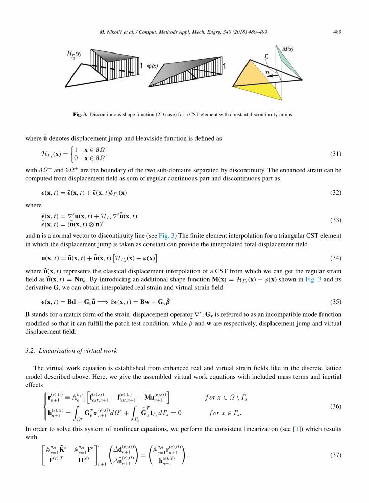
Fig. 3. Discontinuous shape function (2D case) for a CST element with constant discontinuity jumps.

where ¯u denotes displacement jump and Heaviside function is defined as

HΓs (x) =

1 x ∈ ∂Ω−

0 x ∈ ∂Ω+ (31)

with ∂Ω− and ∂Ω+ are the boundary of the two sub-domains separated by discontinuity. The enhanced strain can becomputed from displacement field as sum of regular continuous part and discontinuous part as

ϵ(x, t) = ϵ(x, t) + ¯ϵ(x, t)δΓs (x) (32)

where

ϵ(x, t) = s u(x, t) + HΓss ¯u(x, t)

¯ϵ(x, t) = ( ¯u(x, t) ⊗ n)s (33)

and n is a normal vector to discontinuity line (see Fig. 3) The finite element interpolation for a triangular CST elementin which the displacement jump is taken as constant can provide the interpolated total displacement field

u(x, t) = u(x, t) + ¯u(x, t)[HΓs (x) − ϕ(x)

](34)

where u(x, t) represents the classical displacement interpolation of a CST from which we can get the regular strainfield as u(x, t) = Nua . By introducing an additional shape function M(x) = HΓs (x) − ϕ(x) shown in Fig. 3 and itsderivative G, we can obtain interpolated real strain and virtual strain field

ϵ(x, t) = Bd + Gr ¯u H⇒ ∂ϵ(x, t) = Bw + Gv¯β (35)

B stands for a matrix form of the strain–displacement operator ∇s , Gv is referred to as an incompatible mode function

modified so that it can fulfill the patch test condition, while ¯β and w are respectively, displacement jump and virtualdisplacement field.

3.2. Linearization of virtual work

The virtual work equation is established from enhanced real and virtual strain fields like in the discrete latticemodel described above. Here, we give the assembled virtual work equations with included mass terms and inertialeffects⎧⎪⎨⎪⎩

r(e),(i)n+1 = Anel

e=1

[f(e),(i)ext,n+1 − f(e),(i)

int,n+1 − Ma(e),(i)n+1

]f or x ∈ Ω \ Γs

h(e),(i)n+1 =

∫Ωe

GTv σ

(e),(i)n+1 dΩ e

+

∫Γs

¯GT

v tΓs dΓs = 0 f or x ∈ Γs .(36)

In order to solve this system of nonlinear equations, we perform the consistent linearization (see [1]) which resultswith [

Anele=1Ke Anel

e=1Fe

F(e),T H(e)

]i

n+1

(∆d(e),(i)

n+1

∆ ¯u(e),(i)n+1

)=

(Anel

e=1r(e),(i)n+1

h(e),(i)n+1

). (37)


The embedded strong discontinuity approach allows to exploit the condensation of discontinuity related parametersproducing the final linearized equation

Anele=1(K(e),(i)

e f f,n+1∆d(e),(i)n+1 ) = Anel

e=1r(e),(i)e f f,n+1. (38)

The effective matrix K(e),(i)e f f,n+1 contains the contribution from static condensation due to embedded strong discontinuity,

where element sub-matrices H(e) and F(e) are computed in a similar manner to the one presented in Section 2.Additionally, the effective matrix also contains the contribution from the Newmark algorithm for time integrationin dynamics

K(e),(i)e f f,n+1 = K(e),(i)

n+1 − F(e),(i)n+1 (H(e),(i)

n+1 )−1F(e),(i),Tn+1 +

1(∆t)2β

Me (39)

and residual is computed by subtracting the inertial terms

r(e),(i)e f f,n+1 = r(e),(i)

n+1 − Mea(i)n+1. (40)

3.3. Damage softening

The occurrence of localized failure in enhanced CST element is followed by damage softening constitutive lawfor crack opening. The model is also developed so that it can account for damage hardening behavior, which issummarized in free energy potential defined as

ψ(ϵ, D, ξ ) =12ϵ · D−1ϵ + Ξ (ξ )

ψ(ϵ,D,ξ )

+12

¯u ·¯Q

−1¯u +

¯Ξ ( ¯ξ ) ¯ψ( ¯u, ¯Q, ¯ξ )

δΓs . (41)

We can note that free energy is split into two parts, where the first one concerns the hardening part and the second onesoftening localized part which is introduced by Dirac function. In this work we are interested in localized softeningpart only which occurs when the failure is detected by damage softening function ¯Φ = 0, with no hardening. Here,¯Ξ ( ¯ξ ) = − ¯q ¯ξ and stress-like damage softening variable is defined as exponential function

¯q = ¯σ f

[1 − exp(−

¯β

¯σ f

¯ξ )

]H⇒

¯K = −∂ ¯q

∂ ¯ξ= −

¯βexp(−¯β

¯σ f

¯ξ ). (42)

The softening detection function is defined as

¯Φ(tΓs ,¯q) =

ˆΦ(tΓs ) − ( ¯σ f − ¯q) (43)

whereˆΦ(tΓs ) is a function of degree one containing the traction vector tΓs = (σn)Γs which acts at discontinuity

surface. We can write the loading–unloading conditions and consistency condition

˙γ ≥ 0˙Φ(tΓs ,

¯q) ≤ 0 ˙γ˙Φ(tΓs ,

¯q) = 0. (44)

The damage dissipation in localized softening can be defined as

DP =12

tΓs ·˙QtΓs −

d ¯Ξ ( ¯ξ )

d ¯ξ

˙ξ =

12

tΓs ·˙QtΓs + ¯q

˙ξ . (45)

Similarly to plasticity case described above, the integration of the theorem of expended stress power provides thevalue for fracture energy

G f =

∫∞

0

¯σ f exp(−¯β

¯σ f

¯ξ )d ¯ξ (46)

while damage work WD can be obtained by integrating the expression (46) in the range from zero to current valueof ¯ξ .


Fig. 4. Set up for Kalthoff’s experiment.

4. Numerical simulations

In this section we present the results of numerical simulations. Each simulation deals with problem where localizedfailure with crack initiation and propagation is triggered by impulsive load and where the inertial effects are important.The presented examples include some demanding problems, including Kalthoff’s experiment in which plate with twonotches is subjected to edge impact [38] and dynamic crack branching problem [39]. Simulations are conducted withboth models presented above, which are implemented into research version of the computer code FEAP [40].

4.1. Pre-notched plate subjected to impulsive load—kalthoff’s experiment

In this test, the two notched maraging steel specimen is subjected to the edge impact of a projectile applied inthe direction of the notches (see Fig. 4). The available experimental results for such test, reported in Kalthoff [38](with variation of this test with one notch in Zhou et al. [41]), attracted large interest turning this example into thebenchmark. Namely, numerical computations for the test are conducted with various methods such as XFEM [3–5],ED-FEM [9,10], phase field [11,12] or discrete lattice model [32,33].

Geometry and boundary conditions of the specimen are given in Fig. 4. The projectile impact is represented in themodel by imposed velocity, which is initially applied and held constant. We can consider here only half of the meshdue to the symmetry in order to reduce the computational cost. The initial notch is modeled directly by leaving thespace in the mesh. The material parameters for maraging steel are chosen for model parameters with ρ = 8000 kg/m3,E = 190 GPa and ν = 0.3. The maximal uniaxial tensile stress of σu = 1.07 GPa is considered for threshold valuewhich triggers the failure mechanism in mode I. The other model parameters are fracture energy in mode I chosen asG f,I = 5 × 104 N/m for plasticity model and softening variable βI = 17 GPa/mm chosen for the damage model.We also consider the possible failure in mode II, with model parameters for shear threshold value chosen as τu = 1GPa, fracture energy for mode II in plasticity model G f,I I = 5 × 104 N/m and damage model parameter βI I = 17GPa/mm.

When subjected to edge impulsive load, the maraging steel exhibits failure mode transition. Namely, for lowerloading rates, failure is influenced by mode I tensile crack at an angle of about 70. High loading rates on the contraryproduce failure in mode II by adiabatic shear bands which are experimentally observed in [38].

First we model the case with lower loading rate where we impose constant velocity of v0 = 16.5 m/s at the positionof projectile impact. Three different mesh densities are used for the same experiment and with both models. It shouldbe noted that elements in discrete lattice model mesh are Timoshenko beams, which are positioned at Delaunay edges


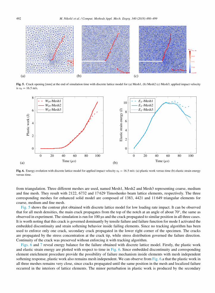
Fig. 5. Crack opening [mm] at the end of simulation time with discrete lattice model for (a) Mesh1, (b) Mesh2 (c) Mesh3; applied impact velocityis v0 = 16.5 m/s.

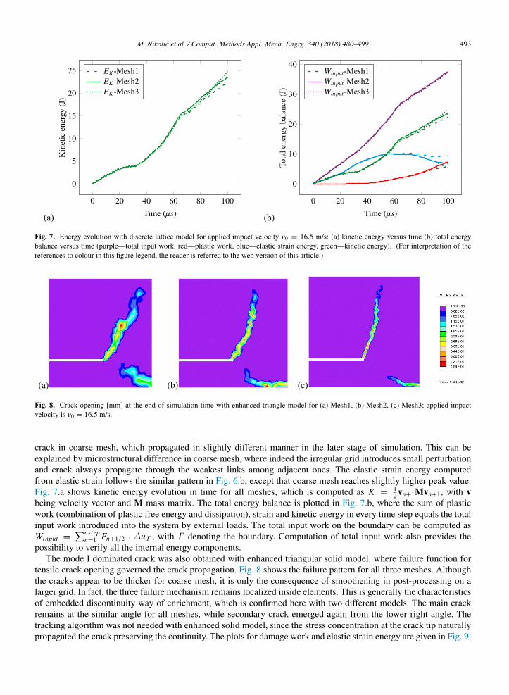
Fig. 6. Energy evolution with discrete lattice model for applied impact velocity v0 = 16.5 m/s: (a) plastic work versus time (b) elastic strain energyversus time.

from triangulation. Three different meshes are used, named Mesh1, Mesh2 and Mesh3 representing coarse, mediumand fine mesh. They result with 2122, 6732 and 17 629 Timoshenko beam lattice elements, respectively. The threecorresponding meshes for enhanced solid model are composed of 1383, 4421 and 11 649 triangular elements forcoarse, medium and fine mesh.

Fig. 5 shows the contour plot obtained with discrete lattice model for low loading rate impact. It can be observedthat for all mesh densities, the main crack propagates from the top of the notch at an angle of about 70, the same asobserved in experiment. The simulation is run for 100 µs and the crack propagated to similar position in all three cases.It is worth noting that this crack is governed dominantly by tensile failure and failure function for mode I activated theembedded discontinuity and strain softening behavior inside failing elements. Since no tracking algorithm has beenused to enforce only one crack, secondary crack propagated in the lower right corner of the specimen. The cracksare propagated by the stress concentration at the crack tip, while stress distribution governed the failure direction.Continuity of the crack was preserved without enforcing it with tracking algorithm.

Figs. 6 and 7 reveal energy balance for the failure obtained with discrete lattice model. Firstly, the plastic workand elastic strain energy are plotted with respect to time in Fig. 6. Since embedded discontinuity and correspondingelement enrichment procedure provide the possibility of failure mechanism inside elements with mesh independentsoftening response, plastic work also remains mesh independent. We can observe from Fig. 6.a that the plastic work inall three meshes remains very close, since cracks propagated until the same position in the mesh and localized failureoccurred in the interiors of lattice elements. The minor perturbation in plastic work is produced by the secondary


Fig. 7. Energy evolution with discrete lattice model for applied impact velocity v0 = 16.5 m/s: (a) kinetic energy versus time (b) total energybalance versus time (purple—total input work, red—plastic work, blue—elastic strain energy, green—kinetic energy). (For interpretation of thereferences to colour in this figure legend, the reader is referred to the web version of this article.)

Fig. 8. Crack opening [mm] at the end of simulation time with enhanced triangle model for (a) Mesh1, (b) Mesh2, (c) Mesh3; applied impactvelocity is v0 = 16.5 m/s.

crack in coarse mesh, which propagated in slightly different manner in the later stage of simulation. This can beexplained by microstructural difference in coarse mesh, where indeed the irregular grid introduces small perturbationand crack always propagate through the weakest links among adjacent ones. The elastic strain energy computedfrom elastic strain follows the similar pattern in Fig. 6.b, except that coarse mesh reaches slightly higher peak value.Fig. 7.a shows kinetic energy evolution in time for all meshes, which is computed as K =

12 vn+1Mvn+1, with v

being velocity vector and M mass matrix. The total energy balance is plotted in Fig. 7.b, where the sum of plasticwork (combination of plastic free energy and dissipation), strain and kinetic energy in every time step equals the totalinput work introduced into the system by external loads. The total input work on the boundary can be computed asWinput =

∑nstepn=1 Fn+1/2 · ∆uΓ , with Γ denoting the boundary. Computation of total input work also provides the

possibility to verify all the internal energy components.The mode I dominated crack was also obtained with enhanced triangular solid model, where failure function for

tensile crack opening governed the crack propagation. Fig. 8 shows the failure pattern for all three meshes. Althoughthe cracks appear to be thicker for coarse mesh, it is only the consequence of smoothening in post-processing on alarger grid. In fact, the three failure mechanism remains localized inside elements. This is generally the characteristicsof embedded discontinuity way of enrichment, which is confirmed here with two different models. The main crackremains at the similar angle for all meshes, while secondary crack emerged again from the lower right angle. Thetracking algorithm was not needed with enhanced solid model, since the stress concentration at the crack tip naturallypropagated the crack preserving the continuity. The plots for damage work and elastic strain energy are given in Fig. 9.


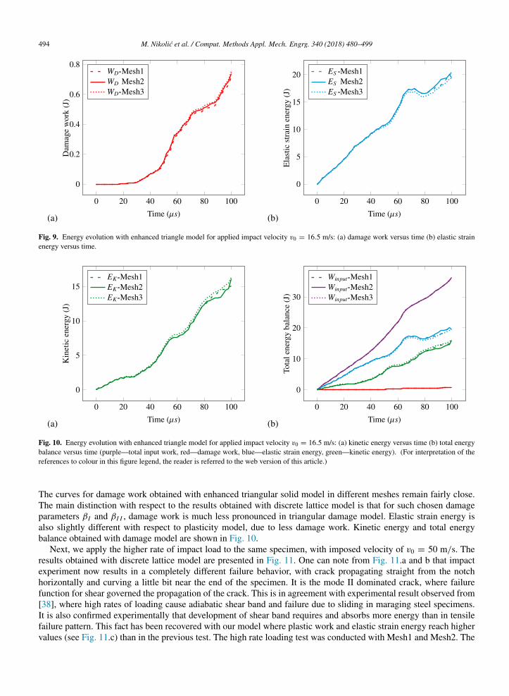
Fig. 9. Energy evolution with enhanced triangle model for applied impact velocity v0 = 16.5 m/s: (a) damage work versus time (b) elastic strainenergy versus time.

Fig. 10. Energy evolution with enhanced triangle model for applied impact velocity v0 = 16.5 m/s: (a) kinetic energy versus time (b) total energybalance versus time (purple—total input work, red—damage work, blue—elastic strain energy, green—kinetic energy). (For interpretation of thereferences to colour in this figure legend, the reader is referred to the web version of this article.)

The curves for damage work obtained with enhanced triangular solid model in different meshes remain fairly close.The main distinction with respect to the results obtained with discrete lattice model is that for such chosen damageparameters βI and βI I , damage work is much less pronounced in triangular damage model. Elastic strain energy isalso slightly different with respect to plasticity model, due to less damage work. Kinetic energy and total energybalance obtained with damage model are shown in Fig. 10.

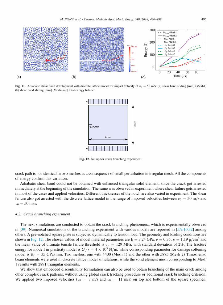
Next, we apply the higher rate of impact load to the same specimen, with imposed velocity of v0 = 50 m/s. Theresults obtained with discrete lattice model are presented in Fig. 11. One can note from Fig. 11.a and b that impactexperiment now results in a completely different failure behavior, with crack propagating straight from the notchhorizontally and curving a little bit near the end of the specimen. It is the mode II dominated crack, where failurefunction for shear governed the propagation of the crack. This is in agreement with experimental result observed from[38], where high rates of loading cause adiabatic shear band and failure due to sliding in maraging steel specimens.It is also confirmed experimentally that development of shear band requires and absorbs more energy than in tensilefailure pattern. This fact has been recovered with our model where plastic work and elastic strain energy reach highervalues (see Fig. 11.c) than in the previous test. The high rate loading test was conducted with Mesh1 and Mesh2. The


Fig. 11. Adiabatic shear band development with discrete lattice model for impact velocity of v0 = 50 m/s: (a) shear band sliding [mm] (Mesh1)(b) shear band sliding [mm] (Mesh2) (c) total energy balance.

Fig. 12. Set up for crack branching experiment.

crack path is not identical in two meshes as a consequence of small perturbation in irregular mesh. All the componentsof energy confirm this variation.

Adiabatic shear band could not be obtained with enhanced triangular solid element, since the crack got arrestedimmediately at the beginning of the simulation. The same was observed in experiment where shear failure gets arrestedin most of the cases and applied velocities. Different thicknesses of the notch are also varied in experiment. The shearfailure also got arrested with the discrete lattice model in the range of imposed velocities between v0 = 30 m/s andv0 = 50 m/s.

4.2. Crack branching experiment

The next simulations are conducted to obtain the crack branching phenomena, which is experimentally observedin [39]. Numerical simulations of the branching experiment with various models are reported in [5,9,10,32] amongothers. A pre-notched square plate is subjected dynamically to tension load. The geometry and loading conditions areshown in Fig. 12. The chosen values of model material parameters are E = 3.24 GPa, ν = 0.35, ρ = 1.19 g/cm3 andthe mean value of ultimate tensile failure threshold is σu = 129 MPa, with standard deviation of 2%. The fractureenergy for mode I in plasticity model is G f,I = 4 × 103 N/m, while corresponding parameter for damage softeningmodel is βI = 35 GPa/mm. Two meshes, one with 4400 (Mesh 1) and the other with 5885 (Mesh 2) Timoshenkobeam elements were used in discrete lattice model simulations, while the solid element mesh corresponding to Mesh1 results with 2891 triangular elements.

We show that embedded discontinuity formulation can also be used to obtain branching of the main crack amongother complex crack patterns, without using global crack tracking procedure or additional crack branching criterion.We applied two imposed velocities (v0 = 7 m/s and v0 = 11 m/s) on top and bottom of the square specimen.


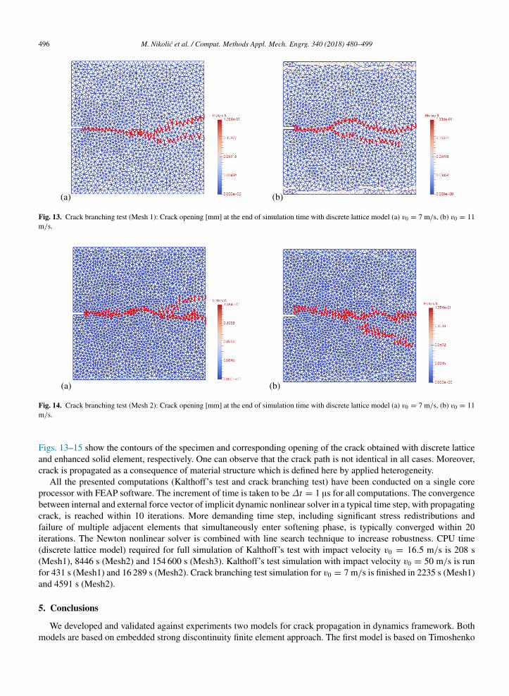
Fig. 13. Crack branching test (Mesh 1): Crack opening [mm] at the end of simulation time with discrete lattice model (a) v0 = 7 m/s, (b) v0 = 11m/s.

Fig. 14. Crack branching test (Mesh 2): Crack opening [mm] at the end of simulation time with discrete lattice model (a) v0 = 7 m/s, (b) v0 = 11m/s.

Figs. 13–15 show the contours of the specimen and corresponding opening of the crack obtained with discrete latticeand enhanced solid element, respectively. One can observe that the crack path is not identical in all cases. Moreover,crack is propagated as a consequence of material structure which is defined here by applied heterogeneity.

All the presented computations (Kalthoff’s test and crack branching test) have been conducted on a single coreprocessor with FEAP software. The increment of time is taken to be ∆t = 1 µs for all computations. The convergencebetween internal and external force vector of implicit dynamic nonlinear solver in a typical time step, with propagatingcrack, is reached within 10 iterations. More demanding time step, including significant stress redistributions andfailure of multiple adjacent elements that simultaneously enter softening phase, is typically converged within 20iterations. The Newton nonlinear solver is combined with line search technique to increase robustness. CPU time(discrete lattice model) required for full simulation of Kalthoff’s test with impact velocity v0 = 16.5 m/s is 208 s(Mesh1), 8446 s (Mesh2) and 154 600 s (Mesh3). Kalthoff’s test simulation with impact velocity v0 = 50 m/s is runfor 431 s (Mesh1) and 16 289 s (Mesh2). Crack branching test simulation for v0 = 7 m/s is finished in 2235 s (Mesh1)and 4591 s (Mesh2).

5. Conclusions

We developed and validated against experiments two models for crack propagation in dynamics framework. Bothmodels are based on embedded strong discontinuity finite element approach. The first model is based on Timoshenko


Fig. 15. Crack branching test: Crack opening [mm] at the end of simulation time with enhanced triangle model (a) v0 = 7 m/s, (b) v0 = 11 m/s.

beam lattice extracted from Voronoi cells, where Timoshenko beams are equipped with embedded discontinuityenhancements to provide failure modes I and II. This model was developed in our earlier works for quasi-static failurein heterogeneous materials. Here, we show that extension to dynamics framework can be upgraded in a straightforwardmanner by adding the inertial contributions without need for changing the existing quasi static model. The secondmodel is based on enhanced triangular solid element, where failure also occurs due to modes I and II. The extensionto dynamics framework is performed in the same way, without any need to change the code for existing quasi staticcase. The presented two models are developed initially for failure in heterogeneous materials and solid structures,respectively.

We conducted the two dynamic crack propagation benchmarks with both models where we could summarize thefeatures of the approach for crack phenomena based on embedded strong discontinuity. Namely, since contributionof embedded strong discontinuity enhancement remains local inside elements, different mesh sizes, and even fairlycoarse grids, could be used to obtain results for presented dynamics benchmarks. The same approach allows to keepthe fixed mesh during the whole simulation, due to crack propagating in the element interiors. These benefits lead tohigh computational efficiency. It is important to note that we did not use any tracking procedure for crack which wouldadditionally increase the computational cost. Namely, tracking the crack path was not the major concern of this work.Instead, we rather focus upon the true energy balance and leave the material structure and complex stress states acrossthe crack tip to govern the crack path. For instance, stress concentration occurring on the top of the notch and crackwould trigger and extend the crack, while stress state and inertial forces orientate the crack in corresponding directions.Complexities, such as multiple cracks with their interaction, are shown to be represented very well. Dynamic crackbranching phenomena can be obtained with both models. The tensile cracks are obtained in the so-called Kalthoff’sexperiment where low rate of the impact load triggers the crack at an angle at about 70 with both models. For highloading rate adiabatic shear band, or mode II crack, is obtained with discrete lattice model. However it could not beobtained with enhanced triangular solid model since the shear crack got arrested soon in the simulation.

The proposed methodology is computationally very efficient with various failure and crack related complexitiesbeing resolved. It can be used for computation of homogeneous solids and heterogeneous materials.

The true benefits of the approach could be used for failure applications in 3D environment where complex cracksbecome surfaces. Their interaction will automatically be resolved like shown in the present 2D case, while at the sametime relatively coarse grids could provide correct failure phenomena all resulting with high computational efficiency.

Acknowledgments

Mijo Nikolic and Zeljana Nikolic would like to thank the Croatian Science Foundation for the funding of thiswork under the project Development of numerical models for reinforced-concrete and stone masonry structures underseismic loading based on discrete cracks (IP-2014-09-2319).

Xuan Nam Do and Adnan Ibrahimbegovic would like to thank the Hauts-de-France Region (CR Picardie)(120-2015-RDISTRUCT-000010 and RDISTRUCT-000010) and the European Regional Development Fund (ERDF)


2014/2020 for Chaire-de-Mecanique (120-2015-RDISTRUCTF-000010 and RDISTRUCTI-000004) for the fundingof this work.

This support is gratefully acknowledged.

References

[1] A. Ibrahimbegovic, Nonlinear Solid Mechanics: Theoretical Formulations and Finite Element Solution Methods, Springer, London, 2009.[2] N. Moes, J. Dolbow, T. Belytschko, A finite element method for crack growth without remeshing, Internat. J. Numer. Methods Engrg. 46

(1999) 131–150.[3] J. Rethore, A. Gravouil, A. Combescure, An energy-conserving scheme for dynamic crack growth using the eXtended finite element method,

Internat. J. Numer. Methods Engrg. 63 (2005) 631–659.[4] Z.L. Liu, T. Menouillard, T. Belytschko, An XFEM/spectral element method for dynamic crack propagation, Int. J. Fract. 169 (2011) 183–198.[5] T. Belytschko, H. Chen, J. Xu, G. Zi, Dynamic crack propagation based on loss of hyperbolicity and a new discontinuous enrichment, Internat.

J. Numer. Methods Engrg. 58 (2003) 1873–1905.[6] N. Moes, T. Belytschko, Extended finite element method for cohesive crack growth, Eng. Fract. Mech. 69 (2002) 813–833.[7] G. Ferte, P. Massin, N. Moes, 3D crack propagation with cohesive elements in the extended finite element method, Comput. Methods Appl.

Mech. Engrg. 300 (2016) 347–374.[8] J.C. Simo, J. Oliver, F. Armero, An analysis of strong discontinuities induced by strain-softening in rate-independent inelastic solids, Comput.

Mech. 12 (1993) 277–296.[9] F. Armero, C. Linder, Numerical simulation of dynamic fracture using finite elements with embedded discontinuities, Int. J. Fract. 160 (2009)

119–141.[10] A.E. Huespe, J. Oliver, P.J. Sanchez, S. Blanco, V. Sonzogni, Strong discontinuity approach in dynamic fracture simulations, Mec. Comput.

25 (2006) 1997–2018.[11] M.J. Borden, C.V. Verhoosel, M.A. Scott, T.J.R. Hughes, C.M. Landis, A phase-field description of dynamic brittle fracture, Comput. Methods

Appl. Mech. Engrg. 217–220 (2012) 77–95.[12] M. Hofacker, C. Miehe, A phase field model of dynamic fracture: Robust field updates for the analysis of complex crack patterns, Internat. J.

Numer. Methods Engrg. 93 (2013) 276–301.[13] J. Oliver, A.E. Huespe, P.J. Sanchez, A comparative study on finite elements for capturing strong discontinuities: E-FEM vs X-FEM, Comput.

Methods Appl. Mech. Engrg. 195 (2006) 4732–4752.[14] M. Nikolic, E. Karavelic, A. Ibrahimbegovic, P. Miscevic, Lattice element models and their peculiarities, Arch. Comput. Methods Eng. (2017).

http://dx.doi.org/10.1007/s11831-017-9210-y.[15] D. Brancherie, A. Ibrahimbegovic, Novel anisotropic continuum-discrete damage model capable of representing localized failure of massive

structures, Eng. Comput. 26 (1/2) (2009) 100–127.[16] X.N. Do, A. Ibrahimbegovic, D. Brancherie, Dynamics framework for 2D anisotropic continuum-discrete damage model for progressive

localized failure of massive structures, Comput. Struct. 183 (2017) 14–26.[17] A. Ibrahimbegovic, E. Wilson, A modified method of incompatible modes, Commun. Appl. Numer. Method 7 (1991) 187–194.[18] M. Nikolic, A. Ibrahimbegovic, P. Miscevic, Brittle and ductile failure of rocks: Embedded discontinuity approach for representing mode I

and mode II failure mechanisms, Internat. J. Numer. Methods Engrg. 102 (2015) 1507–1526.[19] M. Nikolic, A. Ibrahimbegovic, Rock mechanics model capable of representing initial heterogeneities and full set of 3D failure mechanisms,

Comput. Methods Appl. Mech. Engrg. 290 (2015) 209–227.[20] E. Karavelic, M. Nikolic, A. Ibrahimbegovic, A. Kurtovic, A concrete meso-scale model with full set of 3D failure modes with random

distribution of aggregate and cement phase. Part I: formulation and numerical implementation, Comput. Methods Appl. Mech. Engrg. (2017).http://dx.doi.org/10.1016/j.cma.2017.09.013.

[21] M. Nikolic, A. Ibrahimbegovic, P. Miscevic, Discrete element model for the analysis of fluid-saturated fractured poro-plastic medium basedon sharp crack representation with embedded strong discontinuities, Comput. Methods Appl. Mech. Engrg. 298 (2016) 407–427.

[22] E. Hadzalic, A. Ibrahimbegovic, M. Nikolic, Failure mechanisms in coupled poro-plastic medium, Coupled Systems Mechanics 7 (1) (2018)43–59.

[23] E. Schlangen, J.G.M. Van Mier, Simple lattice model for numerical simulation of fracture of concrete materials and structures, Mater. Struct.25 (1992) 534–542.

[24] G. Cusatis, Z. Bazant, L. Cedolin, Confinement-shear lattice CSL model for fracture propagation in concrete, Comput. Methods Appl. Mech.Engrg. 195 (2006) 7154–7171.

[25] P. Grassl, M. Jirasek, Meso-scale approach to modelling the fracture process zone of concrete subjected to uniaxial tension, Internat. J. SolidsStruct. 47 (2010) 957–968.

[26] M. Vassaux, C. Oliver-Leblond, B. Richard, F. Ragueneau, Beam-particle approach to model cracking and energy dissipation in concrete:Identification strategy and validation, Cem. Concr. Compos. 70 (2016) 1–14.

[27] B. Savija, J. Pacheco, E. Schlangen, Lattice modeling of chloride diffusion in sound and cracked concrete, Cem. Concr. Compos. 42 (2013)30–40.

[28] A.S. Sattari, Z.H. Rizvi, H.B. Motra, F. Wuttke, Meso-scale modeling of heat transport in a heterogeneous cemented geomaterial by latticeelement method, Granular Matter 19 (2017) 66.

[29] Z.H. Rizvi, D. Shrestha, A.S. Sattari, F. Wuttke, Numerical modelling of effective thermal conductivity for modified geomaterial using latticeelement method, Heat Mass Transfer 54 (2) (2018) 483–499.

http://refhub.elsevier.com/S0045-7825(18)30310-4/sb1

































http://dx.doi.org/10.1007/s11831-017-9210-y














http://dx.doi.org/10.1016/j.cma.2017.09.013





























[30] B. Savija, E. Schlangen, On the use of a lattice model for analyzing of in-plane vibration of thin plates, Computers. Materials & Continua 48(2015) 181–202.

[31] M. Attar, A. Karrech, K. Regenauer-Lieb, Non-linear modal analysis of structural components subjected to unilateral constraints, J. SoundVib. 389 (2017) 380–410.

[32] M. Braun, J. Fernandez-Saez, A 2D discrete model with a bilinear softening constitutive law applied to dynamic crack propagation problems,Int. J. Fract. 197 (2016) 81–97.

[33] L. Kosteski, R.B. D’Ambra, I. Iturrioz, Crack propagation in elastic solids using the truss-like discrete element method, Int. J. Fract. 174(2012) 139–161.

[34] G.A. D’Addetta, F. Kun, E. Ramm, H.J. Herrmann, From solids to granulates - Discrete element simulations of fracture and fragmentationprocesses in geomaterials, in: P.A. Vermeer, S. Diebels, W. Ehlers, H.J. Herrmann, S. Luding, E. Ramm (Eds.), Continuous and DiscontinuousModelling of Cohesive Frictional Materials, Springer, Berlin, 2001, pp. 231–258.

[35] A. Ibrahimbegovic, A. Delaplace, Microscale and mesoscale discrete models for dynamic fracture of structures built of brittle material,Comput. & Structures 81 (2003) 1255–1265.

[36] H. Yang, S.S. Sinha, Y. Feng, D.B. McCallen, B. Jeremic, Energy dissipation analysis of elastic-plastic materials, Comput. Methods Appl.Mech. Engrg. 331 (2018) 309–326.

[37] P. Rosakis, A.J. Rosakis, G. Ravichandran, J. Hodowany, A thermodynamic internal variable model for the partition of plastic work into heatand stored energy in metals, J. Mech. Phys. Solids 48 (2000) 581–607.

[38] J.F. Kalthoff, Modes of dynamic shear failure in solids, Int. J. Fract. 101 (2000) 1–31.[39] K. Ravi-Chandar, W.G. Knauss, An experimental investigation into dynamic fracture: III On steady-state crack propagation and crack

branching, Int. J. Fract. 26 (1984) 141–154.[40] R.L. Taylor, FEAP Finite element Analysis Program. University of California, Berkeley, http://www.ce.berkeley.edu.rlt.[41] M. Zhou, A.J. Rosakiss, G. Ravichandran, Dynamically propagating shear bands in impact-loaded prenotched plates - I. Experimental

investigations of temperature signatures and propagating speed, J. Mech. Phys. Solids 44 (1996) 981–1006.































http://www.ce.berkeley.edu.rlt

































Date post:	18-Oct-2021
Category:	Documents
Upload:	others
View:	0 times
Download:	0 times

Crack propagation in dynamics by embedded strong ...

Documents