CRANFIELD UNIVERSITY OKEREKE, NDUBUISI UCHECHUKWU ...

CRANFIELD UNIVERSITY

OKEREKE, NDUBUISI UCHECHUKWU

NUMERICAL PREDICTION AND MITIGATION OF SLUGGING

PROBLEMS IN DEEPWATER PIPELINE-RISER SYSTEMS

SCHOOL OF ENERGY, ENVIRONMENT AND AGRIFOOD (SEEA)

OIL & GAS ENGINEERING CENTRE

PhD

Academic Year: 2012 - 2015

SUPERVISOR: DR. FUAT KARA

CO-SUPERVISOR: PROFESSOR JOHN E. OAKEY

9th NOVEMBER, 2015

CRANFIELD UNIVERSITY

SCHOOL OF ENERGY, ENVIRONMENT AND AGRIFOOD (SEEA)

OIL & GAS ENGINEERING CENTRE

PhD

Academic Year: 2012 - 2015

OKEREKE, NDUBUISI UCHECHUKWU

NUMERICAL PREDICTION AND MITIGATION OF SLUGGING

PROBLEMS IN DEEPWATER PIPELINE-RISER SYSTEMS

SUPERVISOR: DR. FUAT KARA

CO-SUPERVISOR: PROFESSOR JOHN E. OAKEY

NOVEMBER, 2015

This thesis is submitted in partial fulfilment of the requirements for

the degree of PhD

© Cranfield University 2015. All rights reserved. No part of this

publication may be reproduced without the written permission of the

copyright owner.

iii

ABSTRACT

Slugging involves pressure and flowrate fluctuations and poses a major threat to

optimising oil production from deepwater reserves. Typical production loss could be as

high as 50%, affecting the ability to meet growing energy demand.

This work is based on numerical simulation using OLGA (OiL and GAs) a one-

dimensional and two-fluid equations based commercial tool for the simulation and

analysis of a typical field case study in West Africa. Numerical model was adopted for

the field case. Based on the field report, Flow Loop X1 consisted of well X1 and well X2,

(where X1 is the well at the inlet and X2 is the well connected from the manifold (MF)).

Slugging was experienced at Flow Loop X1 at 3000 BoPD; 4MMScf/D and 3%W/C. This

study investigated the conditions causing the slugging and the liquid and gas phase

behaviour at the period slugging occurred.

The simulation work involved modelling the boundary conditions (heat transfer, ambient

temperature, mass flowrate e.t.c). Also critical was the modelling of the piping diameter,

pipe length, wall thickness and wall type material to reflect the field geometry.

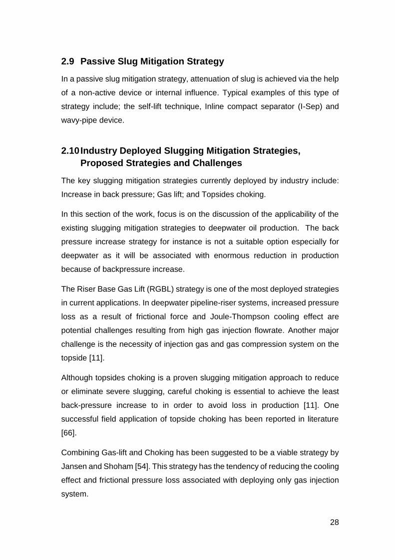
Work on flow regime transition chart showed that slugging became more significant from

30% water-cut, especially at the riser base for a downward inclined flow on the pipeline-

riser system.

Studies on diameter effect showed that increasing diameter from 8” – 32” gave rise to a

drop in Usg (superficial velocity gas) and possible accumulation of liquids on the riser-

base position and hence a tendency for slugging formation. Depth effect study showed

that increasing depth gave rise to increasing pressure fluctuation, especially at the riser-

base.

Studies on the Self-Lift slug mitigation approach showed that reducing the internal

diameter of the Self-lift by-pass pipe was effective in mitigating slug flow.

S3 (Slug suppression system) was also investigated for deepwater scenario, with the

results indicating a production benefit of 12.5%.

In summary, the work done identified water-cut region where pipeline-riser systems

become more susceptible to slugging. Also, two key up-coming slug mitigation strategies

were studied and their performance evaluated in-view of production enhancement.

iv

Keywords:

Slugging, Prediction, Mitigation, Pipeline-Riser and Deepwater

v

ACKNOWLEDGEMENTS

Firstly, I will like to specially appreciate my supervisors; Dr. Fuat Kara and Prof.

John Oakey for the privilege of working with them on this research. I also seize

this medium to appreciate Petroleum Technology Development Fund (PTDF)

for funding this project. I am deeply indebted to my parents (Eze and Ugo Eze

G.O. Okereke and my siblings (‘Buchi, Chii-Chii, Ijeoma and Ugochi) for their

unflinching support in achieving the goal of this PhD.

To my Wife and Princess (Okereke, Confidence ‘Budo), your exceptional

understanding especially at the tail end of this research with the extra hours I

had to spend away from home is note-worthy. God bless you.

DPR (Department of Petroleum Resources) and Chevron Nigeria Limited are

highly appreciated for providing data for this work.

My appreciation also goes out to Adefemi, Israel and Oyewale, Mayowa for their

contribution towards the development of this work. I will also like to

acknowledge Keith Hurley of IT department for his support even at odd hours.

I also wish to express my sincere appreciation to some research colleagues;

Sunday Kanshio, Dr. Adegboyega Ehinmowo, Dr. Adedipe and Aliyu Aliyu for

the engaging interaction we had in the course of this work.

I am deeply indebted to the HFCC and CPA family especially; Rev. ‘Biyi Ajala,

Dr. Adesola, Sola, Dr. Crisppin Allison, Dr. Gareth, Dr. Patrick, Dr. Michael

Adegbite, Dr. Isaac Ogazi, Dr. Daniel Kamunge, Dr. Ofem, Johnbull and so

many others too numerous to mention. God bless this family of love.

My sincere appreciation also goes to Sam Kabari for making out time to support

the formatting and finishing touch on this work.

To my son “Emmanuel Uchechukwu Okereke”, many thanks for inspiring me to

press forward in order to secure a better future for the family.

To God be the glory, for the successful outcome of this research.

vii

TABLE OF CONTENTS

ABSTRACT ........................................................................................................ iii

ACKNOWLEDGEMENTS................................................................................... v

LIST OF FIGURES ............................................................................................ xii

LIST OF TABLES ........................................................................................... xviii

LIST OF ABBREVIATIONS AND GLOSSARY ................................................. xix

LIST OF SYMBOLS ....................................................................................... xxiii

LIST OF EQUATIONS ..................................................................................... xxv

1 Introduction ................................................................................................. 1

1.1 Background and Motivation for the Study ............................................ 1

1.2 Previous Research ............................................................................... 4

1.3 Gap in Knowledge ................................................................................ 5

1.5 Research Aim and Objectives .............................................................. 7

1.6 Thesis Structure ................................................................................... 7

1.6.1 Publications................................................................................... 9

2 Literature Review ...................................................................................... 11

2.1 Background on Multiphase Flow and Flow Assurance ....................... 11

2.2 Slugging ............................................................................................. 11

2.3 Severe Slugging ................................................................................. 12

2.3.1 Slug Generation .......................................................................... 12

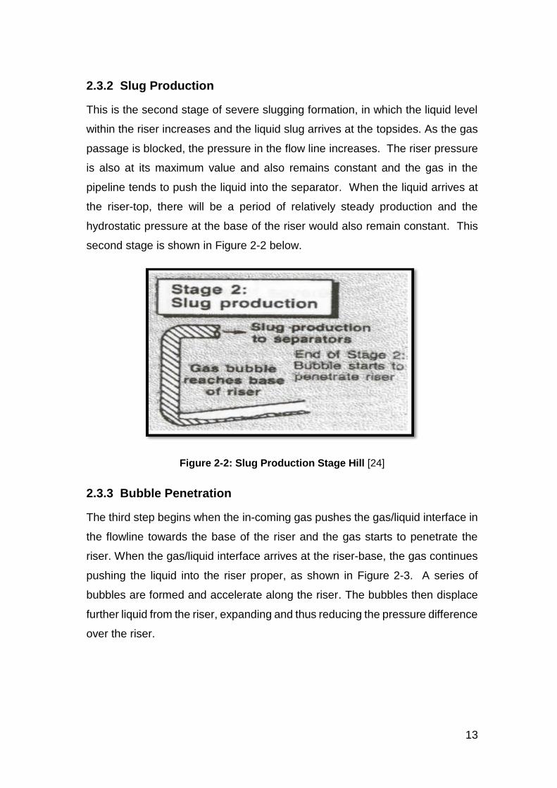
2.3.2 Slug Production ........................................................................... 13

2.3.3 Bubble Penetration ..................................................................... 13

2.3.4 Gas Blow Down and Liquid Fall Back ......................................... 14

2.4 Hydrodynamic Slugging ..................................................................... 15

2.5 Slug Flow Characteristics ................................................................... 16

2.5.1 Liquid Holdup .............................................................................. 16

2.5.2 Gas Holdup ................................................................................. 17

2.5.3 Pressure Drop ............................................................................. 17

2.5.4 Slug Length ................................................................................. 18

2.5.5 Slug Frequency ........................................................................... 18

2.5.6 Slug Period ................................................................................. 18

2.5.7 Slug Velocity ............................................................................... 18

2.5.8 Slug Density ................................................................................ 18

2.6 Slug Flow Behaviour and Prediction .................................................. 19

2.7 Slugging Elimination ........................................................................... 22

2.8 Active Slug Mitigation Strategy........................................................... 27

2.9 Passive Slug Mitigation Strategy ........................................................ 28

2.10 Industry Deployed Slugging Mitigation Strategies, Proposed

Strategies and Challenges ............................................................................ 28

2.11 Upcoming Strategies .......................................................................... 30

viii

2.12 Self-Lifting Technique ........................................................................ 30

2.13 Slug Suppression System .................................................................. 32

2.14 Flow Regime Transition ..................................................................... 35

2.15 Flow Rate Influence on Flow Regime ................................................. 36

2.16 Geometry Influence on Flow Regime ................................................. 38

2.17 Flow Pattern Transition Modelling ...................................................... 38

2.18 Low Mass Flowrate Issue ................................................................... 39

2.19 Diameter Effect Study ........................................................................ 39

2.20 Depth Effect Study ............................................................................. 41

2.21 Field Experience: Gas Surging, a New Deepwater Slug Control

Issue 41

2.22 Summary ............................................................................................ 41

3 Methodology .............................................................................................. 43

3.1 Numerical Modelling ........................................................................... 43

3.2 Background on OLGA (OiL and GAs) ................................................ 44

3.2.1 PVTSim (Fluid Package) – Fluid Properties ................................ 49

3.2.2 Assumptions Made For the OLGA Models .................................. 49

3.2.3 Limitations of OLGA in the Modelling of Cases ........................... 49

3.3 Justification for Methodology .............................................................. 52

3.4 Validation of Modelling Tool ............................................................... 52

3.4.1 Steady State Convergence ......................................................... 53

3.4.2 Steady State Results for Horizontal, Inclined < 400 and Vertical . 54

3.4.3 Pressure Drop per Metre Comparisons for Inclination Angle (00-

900) 55

3.4.4 Transient State Convergence ..................................................... 56

3.5 Liquid Holdup ..................................................................................... 58

3.6 Field Data Description and Validation: ............................................... 60

3.6.1 Model .......................................................................................... 60

3.6.2 Boundary Conditions ................................................................... 61

3.6.3 Fluid Composition ....................................................................... 61

3.7 Approach for Self-lift Study ................................................................ 67

3.8 Approach for S3 Study ....................................................................... 68

3.9 Summary of Validation of Modelling Tool ........................................... 68

4 Field Data/Industry Interaction .................................................................. 71

4.1 Field Data Sourcing ............................................................................ 71

4.2 Preliminary Study on Egina Case ....................................................... 72

4.2.1 Background ................................................................................. 72

4.2.2 Egina North Flow Loop Model ..................................................... 72

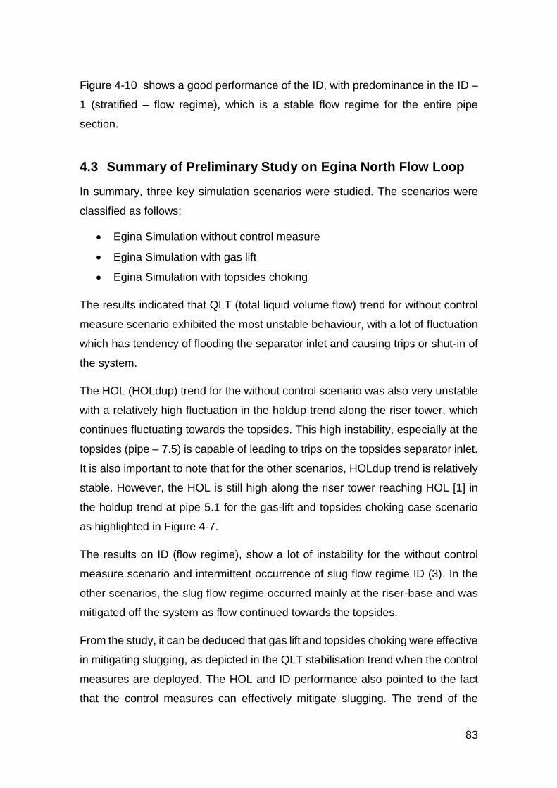
4.3 Summary of Preliminary Study on Egina North Flow Loop ................ 83

4.4 Flow Loop X1 OLGA Model Based On Flow at 3000 BoPD and 6722

BoPD; 4 MMScf/D; 3% WC ........................................................................... 85

4.4.1 Flow Loop X1 Base Case Model ................................................. 85

ix

4.4.2 Fluid Description ......................................................................... 86

4.5 Boundary Condition ............................................................................ 86

4.6 Field Data Validation: Field Data Vs Simulation Comparison ............. 87

4.7 Results for Analysis ............................................................................ 87

4.8 Work On 3000 Bopd, 4MMscf/D and 3% W/C Case ......................... 89

4.9 Work on at 6722 BoPD (Water-cut Sensitivity) .................................. 91

4.10 Limitations on Existing Transition Maps ............................................. 95

4.11 Flow Regime Transition ..................................................................... 95

4.11.1 Stratified-Slug Flow Transition Theoretical Background ............. 95

4.11.2 Further Work on Flow Regime Transition Chart .......................... 96

4.11.3 Impact of Water-Cut on Transition ............................................ 102

4.11.4 Impact of Temperature on Transition ........................................ 102

4.11.5 Impact of Pipeline Inclination on Transition ............................... 103

4.12 Summary of Case Studies and Transition Chart: ............................. 103

5 Adapting Self-lifting Technique to Flow Loop X1 ..................................... 104

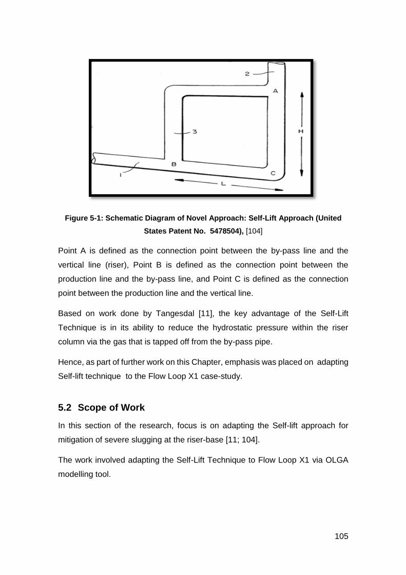
5.1 Self-lift Technique (Background Study) ............................................ 104

5.2 Scope of Work.................................................................................. 105

5.3 Numerical Models ............................................................................ 106

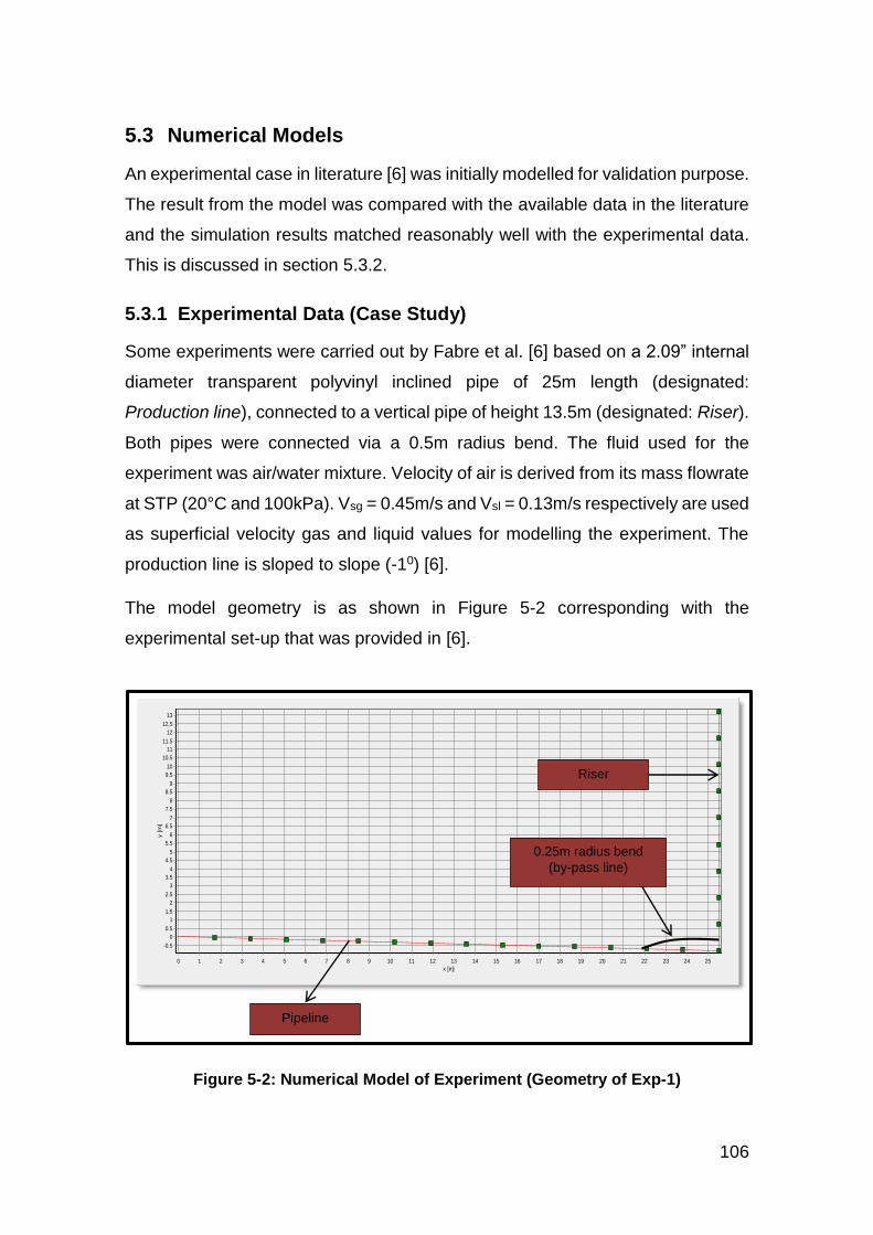
5.3.1 Experimental Data (Case Study) ............................................... 106

5.3.2 Experimental Data (Validation) ................................................. 108

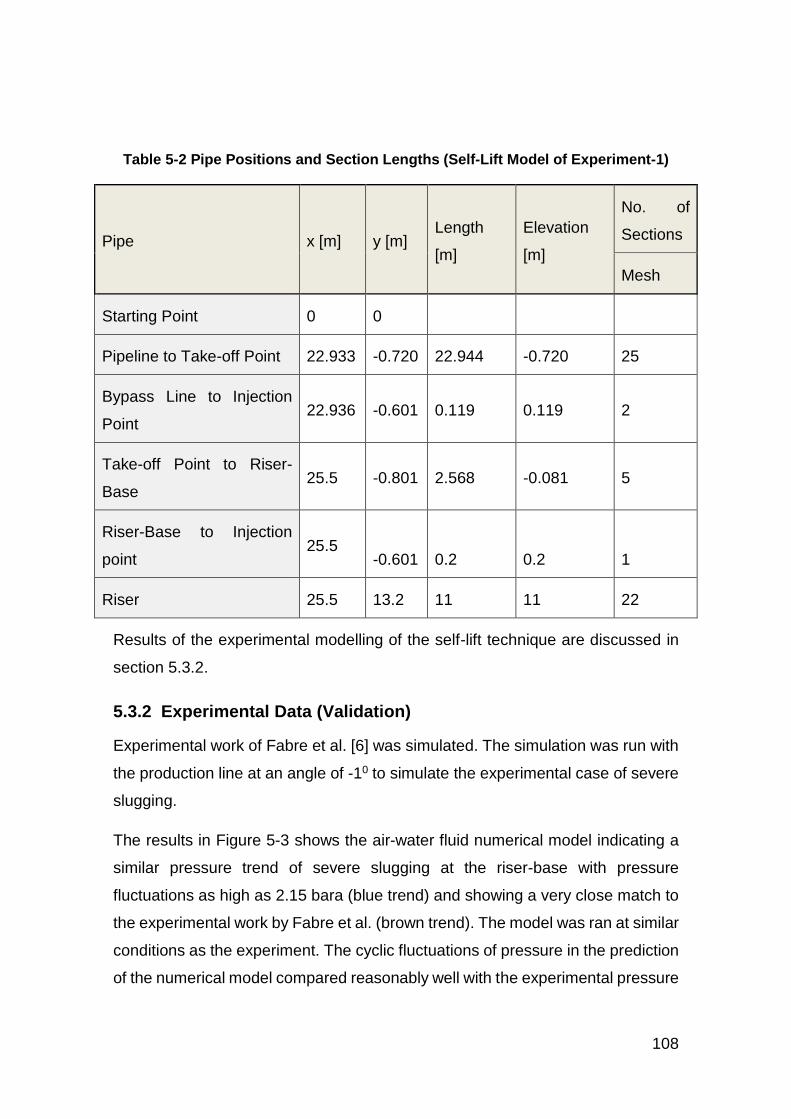
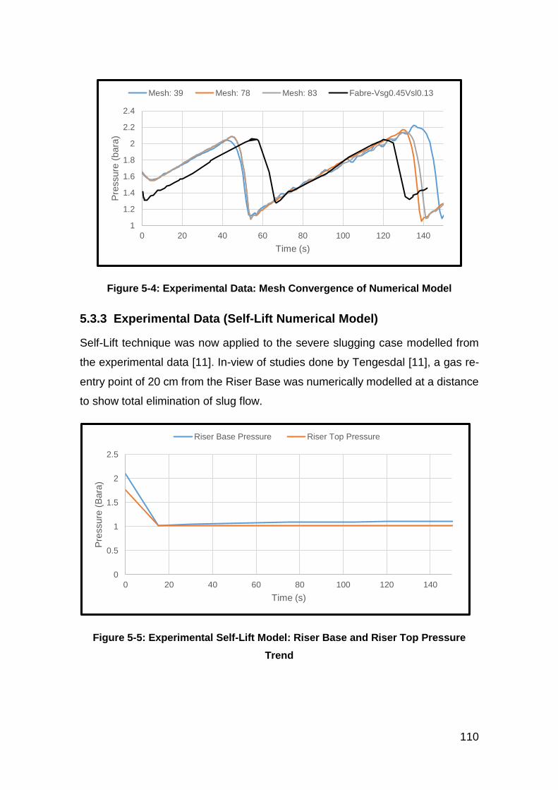
5.3.3 Experimental Data (Self-Lift Numerical Model) ......................... 110

5.3.4 Field Data (Background) ........................................................... 114

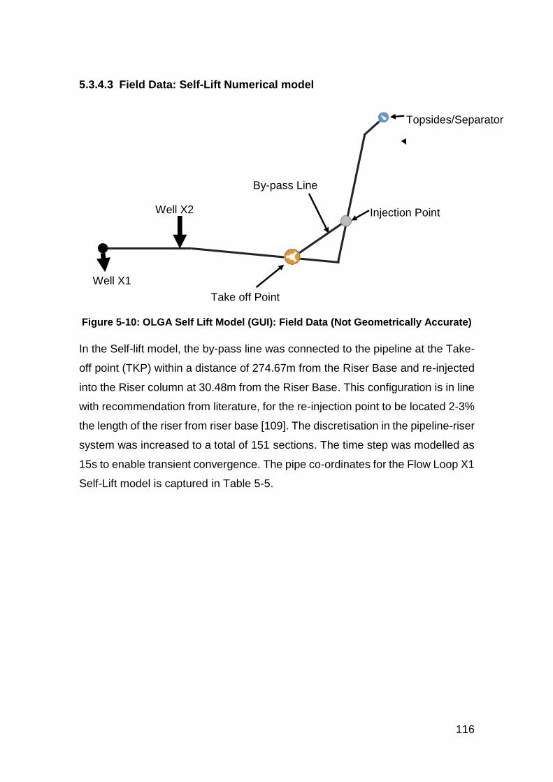
5.4 Results and Discussion (Self-lift Field Data Study) .......................... 117

5.5 Field Data (Flow Loop X1): Slugging ................................................ 117

5.5.1 Modified Field Data (Severe Slugging) ..................................... 118

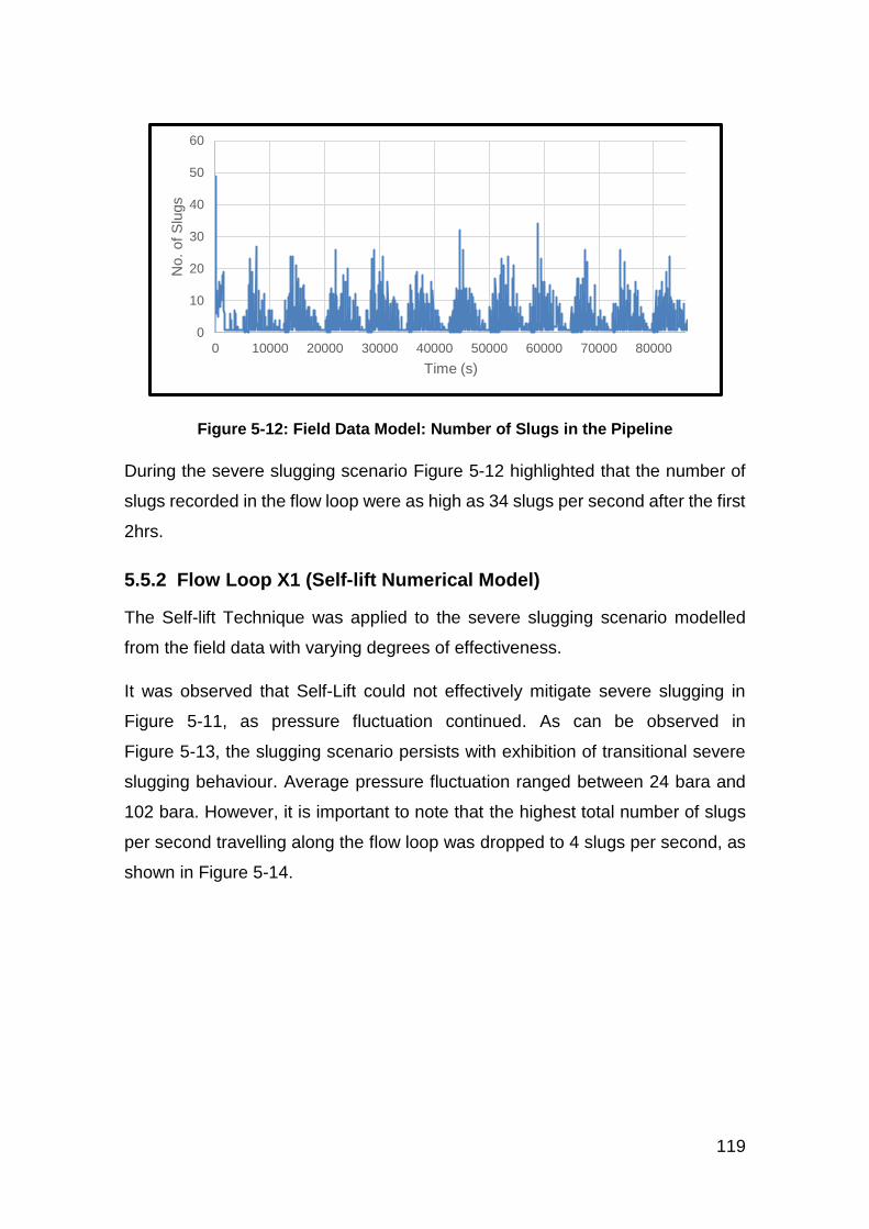
5.5.2 Flow Loop X1 (Self-lift Numerical Model) .................................. 119

5.5.3 Flow Loop X1 (Combination of Self-lift and Gas Injection) ........ 121

6 Adapting S3 (Slug Suppression System) to Flow Loop X1 ...................... 125

6.1 Model ............................................................................................... 125

6.1.1 Fluid Composition ..................................................................... 125

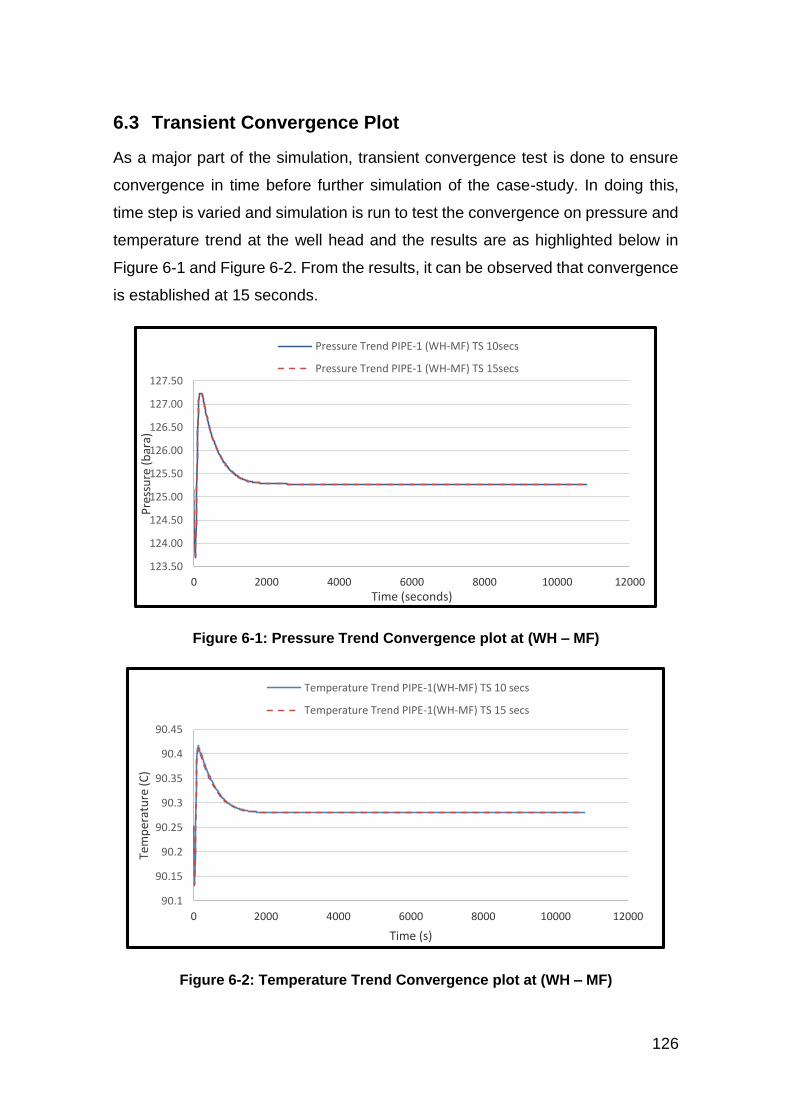
6.2 Transient State Simulation ............................................................... 125

6.3 Transient Convergence Plot ............................................................. 126

6.4 Sensitivity Analysis ........................................................................... 127

6.4.1 Pipeline section adjustment ...................................................... 127

6.5 Results and Discussion .................................................................... 128

6.5.1 Scenario 1 (Source 1 Reducing with Source 2 Shutoff) ............ 128

6.5.2 Scenario 2 (Source 1 Decreasing with Source 2 Constant) ...... 131

6.5.3 Scenario 3 (Source 1 Constant with Source 2 Reducing) ......... 135

6.5.4 Scenario 4 (Both Source 1 and Source 2 Reducing) ................ 137

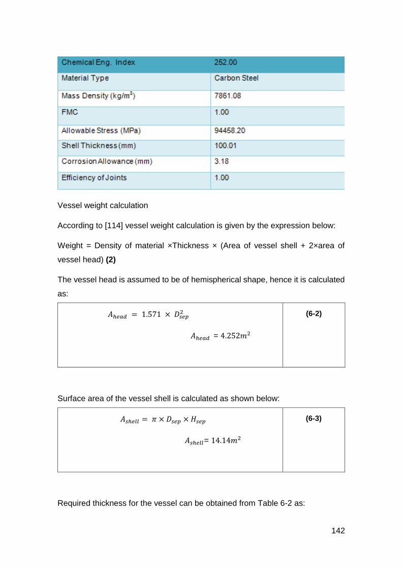
6.6 Applying Slug Suppression System - The Mini Separator ................ 140

6.7 Separator Design ............................................................................. 140

6.8 Controller Tuning .............................................................................. 144

x

6.9 Control Results................................................................................. 144

6.10 Topside Choking .............................................................................. 148

6.11 Summary (Adaptation of S3 to Flow Loop X1) .................................. 150

7 Diameter and Depth Effect Study ............................................................ 151

7.1 Use of Pipes of 6” Internal Diameter ................................................ 154

7.2 Increasing Depth – Increasing Diameter Effect Simulation Results

and Discussion ........................................................................................... 155

7.2.1 Summary .................................................................................. 160

8 Conclusions and Further Work ................................................................ 161

8.1 Summary of Research Aim and Objectives ...................................... 161

8.1.1 Objective 1 and Findings .......................................................... 161






8.2 Contributions to Knowledge ............................................................. 164

8.3 Implications of the Research ............................................................ 164

8.4 Limitations of the Research .............................................................. 166

8.5 Further Work .................................................................................... 167

9 REFERENCES ........................................................................................ 168

10 APPENDICES ..................................................................................... 178

10.1 Appendix A: Three Phase.tab Fluid Composition ............................. 178

10.2 Appendix B: Steady State Holdup and Pressure Drop Correlation

Calculation for Horizontal Case .................................................................. 180

10.3 Appendix C: Steady State Holdup and Pressure Drop Correlation

Calculation for Pipe Inclination 400 ............................................................. 184

10.4 Appendix D: Steady State Holdup and Pressure Drop Correlation


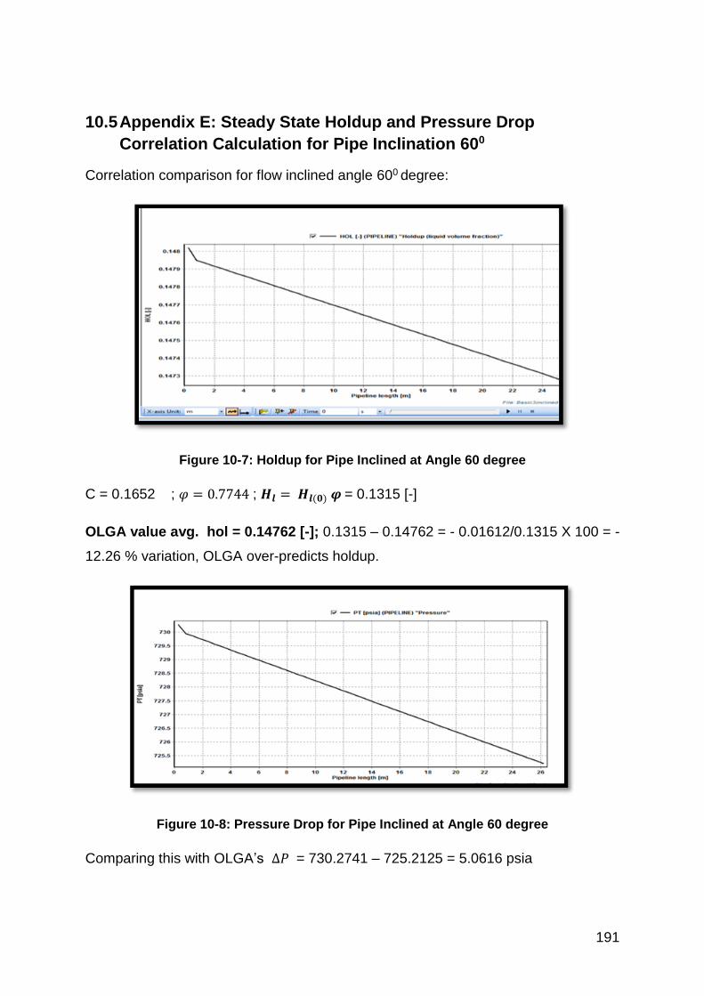
10.5 Appendix E: Steady State Holdup and Pressure Drop Correlation


10.6 Appendix F: Steady State Holdup and Pressure Drop Correlation


10.7 Appendix G: Steady State Holdup and Pressure Drop Correlation


10.8 Appendix H: Steady State Holdup and Pressure Drop Correlation


10.9 Appendix I: Transient Holdup and Pressure Drop Results at

Convergence with Pipe Inclination (500 to 800) ........................................... 201

10.10 Appendix J: Volumetric Flowrate Conversion – Well X1 ............... 205

10.11 Appendix K: Volumetric Flowrate Conversion – Well X2 .............. 206

xi

10.12 Appendix L: Conversion of Volumetric Flowrates to Mass

Flowrates in Phases for Self-lift Model ........................................................ 207

10.13 Appendix M: Fabre et al. Experimental Data Result ..................... 209

10.14 Appendix N: Self-Lift Adapted to Field Data - Results .................. 210

10.15 Appendix O: S3 Convergence Test - Pressure ............................. 212

10.16 Appendix P: Generic Pipeline-Riser Flow Loop ............................ 214

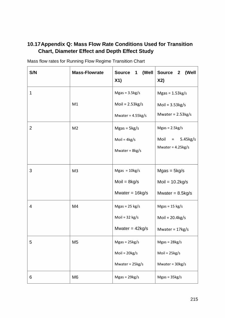
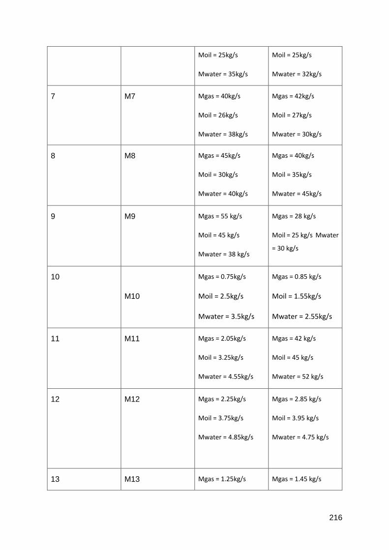
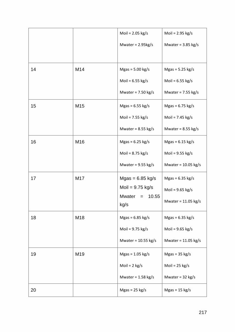
10.17 Appendix Q: Mass Flow Rate Conditions Used for Transition

Chart, Diameter Effect and Depth Effect Study ........................................... 215

10.18 Appendix R: Flow Regime Transition Chart at 50% WC and 60%

WC 220

10.19 Appendix S: Diameter Effect Study at M2 (Mass flow-rate

condition) .................................................................................................... 223

10.20 Appendix T: Typical Power Consumption for Compression and

Production Comparison .............................................................................. 224

xii

LIST OF FIGURES

Figure 1-1: Energy Market Driver [1] .................................................................. 1

Figure 2-1: Slug Generation Stage Hill [24] ...................................................... 12

Figure 2-2: Slug Production Stage Hill [24] ...................................................... 13

Figure 2-3: Bubble Penetration Stage Hill [24] ................................................. 14

Figure 2-4: Gas Blow-Down Stage Hill [24] ...................................................... 15

Figure 2-5: Slug Flow Formation in an Inclined Pipe (Oil & Water Mixtures) [50] .................................................................................................................. 20

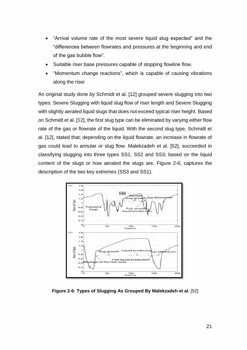
Figure 2-6: Types of Slugging As Grouped By Malekzadeh et al. [52] ............. 21

Figure 2-7: Self-Lift Slugging Elimination Strategy [17] .................................... 31

Figure 2-8: Measurements Indicating Slugging Problem [71] ........................... 33

Figure 2-9: S3 (Slug Suppression System) between A Pipeline Outlet and a First Stage Separator [16] ................................................................................. 34

Figure 2-10: Horizontal Flow Regime Transition Map [4] ................................. 35

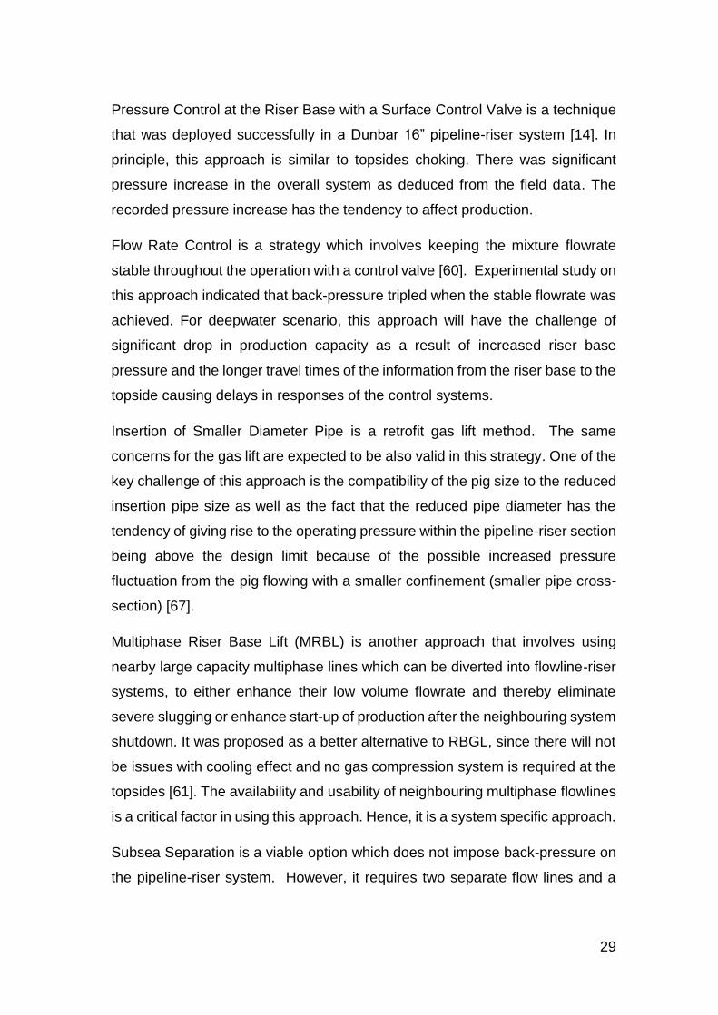
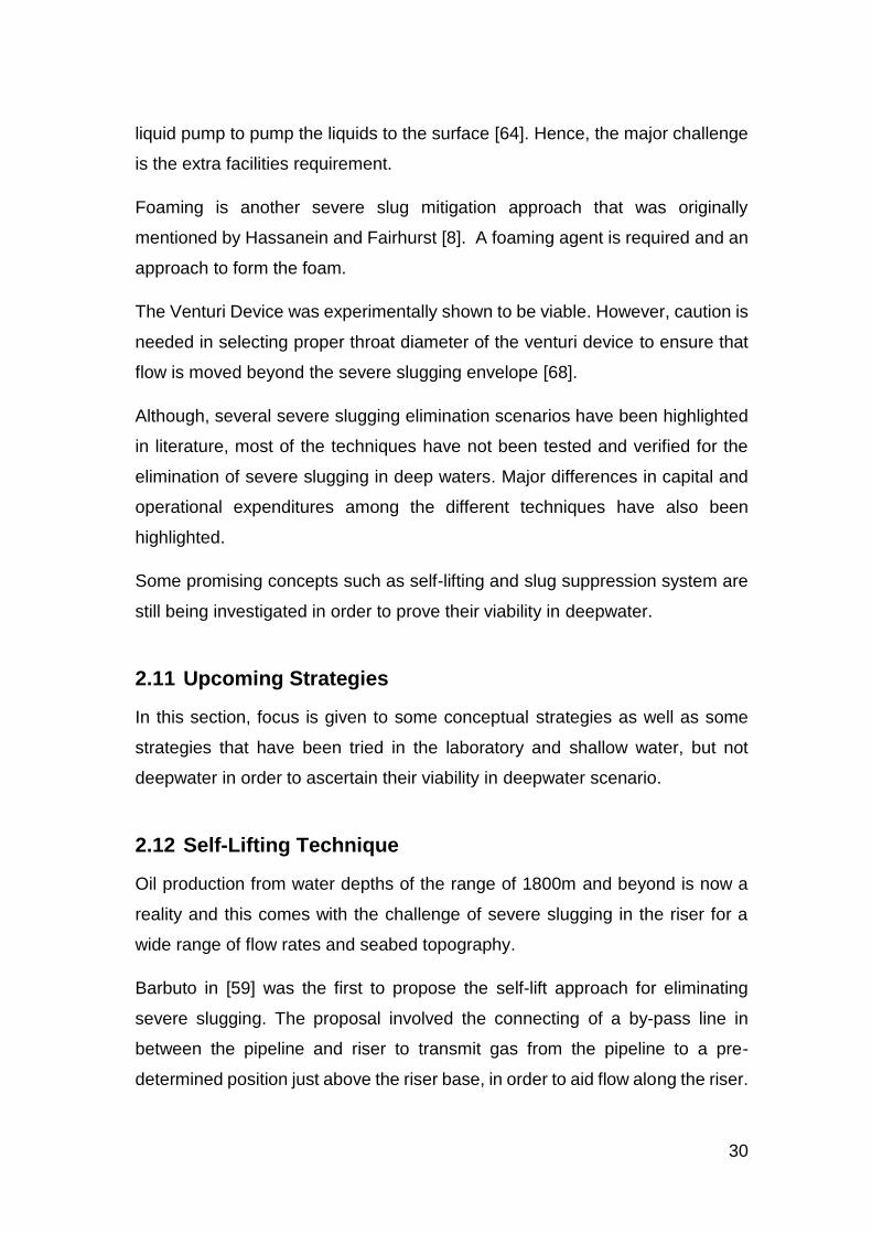
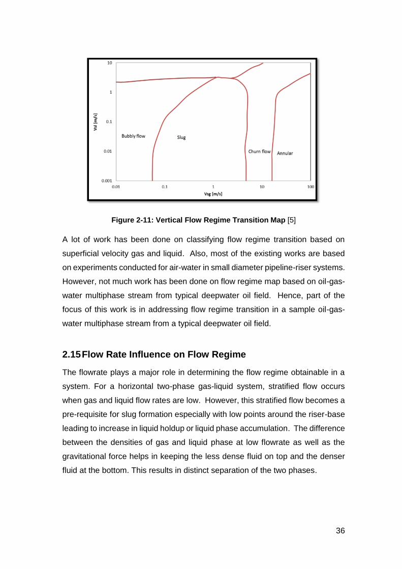
Figure 2-11: Vertical Flow Regime Transition Map [5] ...................................... 36

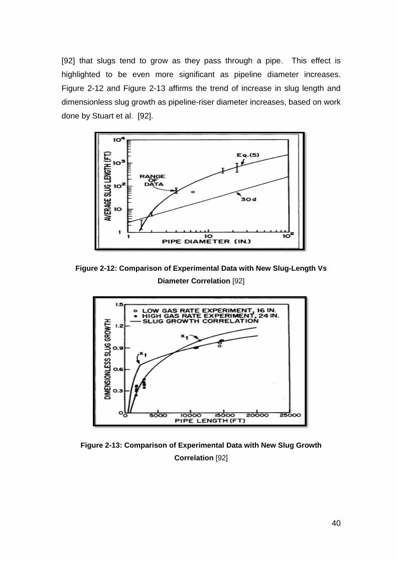
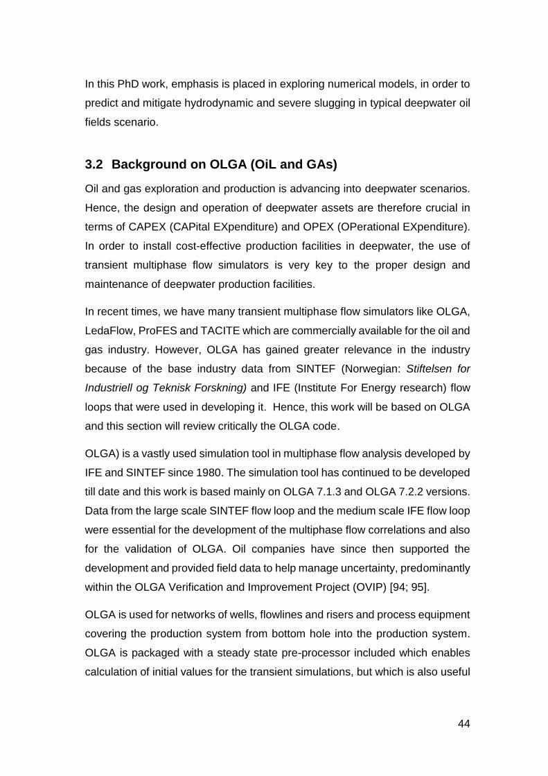
Figure 2-12: Comparison of Experimental Data with New Slug-Length Vs Diameter Correlation [92] .......................................................................... 40

Figure 2-13: Comparison of Experimental Data with New Slug Growth Correlation [92] ............................................................................................................ 40

Figure 3-1: Pressure Fluctuations of Severe Slugging in Horizontal Pipeline-Vertical Riser System Taken from Schimdt et al. [86] Data with OLGA Predictions ................................................................................................ 45

Figure 3-2: Research Flow Chart ..................................................................... 51

Figure 3-3: Steady State Holdup Convergence Test Plot ................................. 53

Figure 3-4: Steady State Pressure Drop Convergence Test Plot ..................... 54

Figure 3-5: Horizontal 20m Pipeline at Steady State ........................................ 55

Figure 3-6: OLGA Pressure Drop per Metre Matched Against Correlation Results and Boussen Experimental Data ............................................................... 56

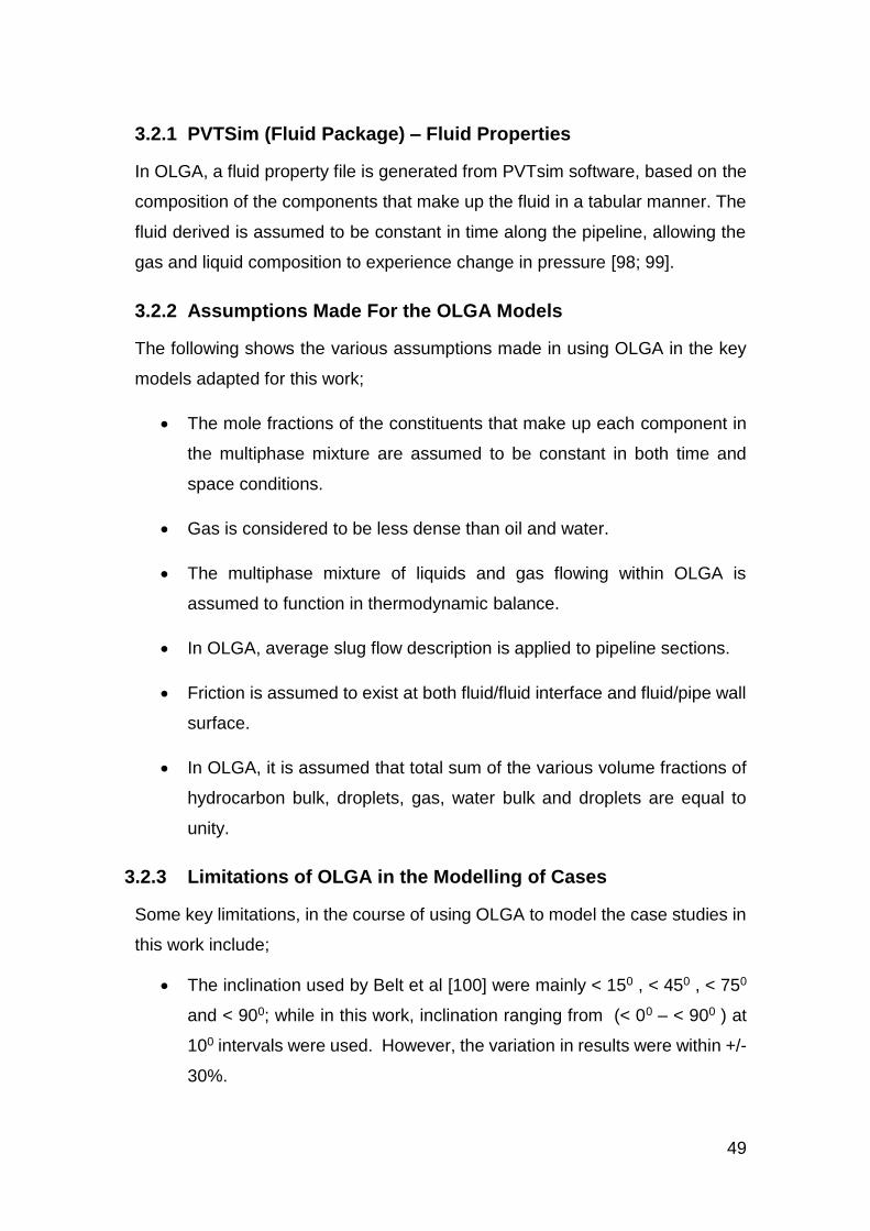
Figure 3-7: Transient Pressure Convergence at (Pipe Section 1.1 - Inlet) ....... 57

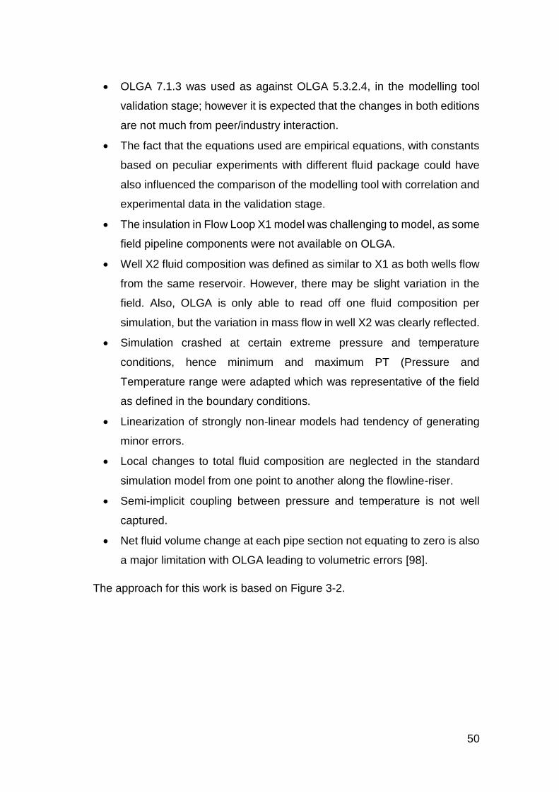
Figure 3-8: Transient Pressure Convergence at (Pipe Section 1.50 – Outlet) .. 57

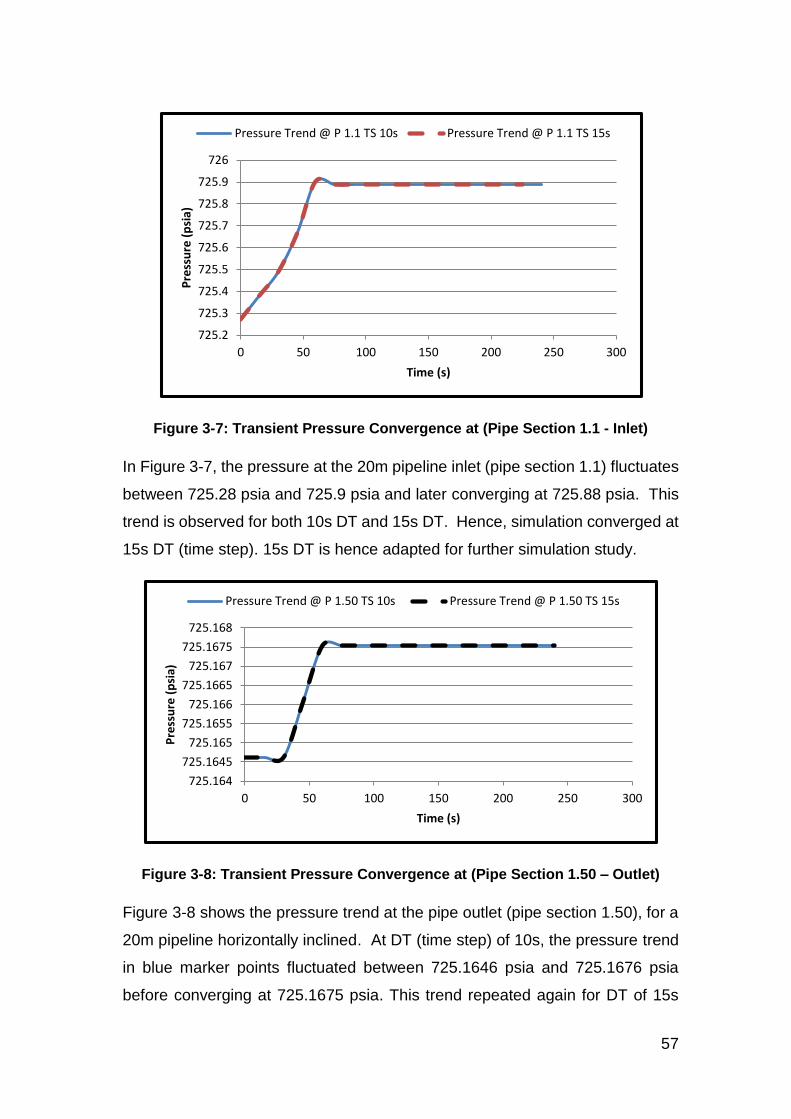
Figure 3-9: Transient Holdup Convergence at (Pipe Section 1.1 – Inlet) ......... 58

Figure 3-10: Comparison of Gregory et al. Correlation Vs Simulation .............. 59

xiii

Figure 3-11: Geometry of Flow Loop X1 Pipeline-Riser System Showing the Profile from Seabed to Topside ................................................................. 63

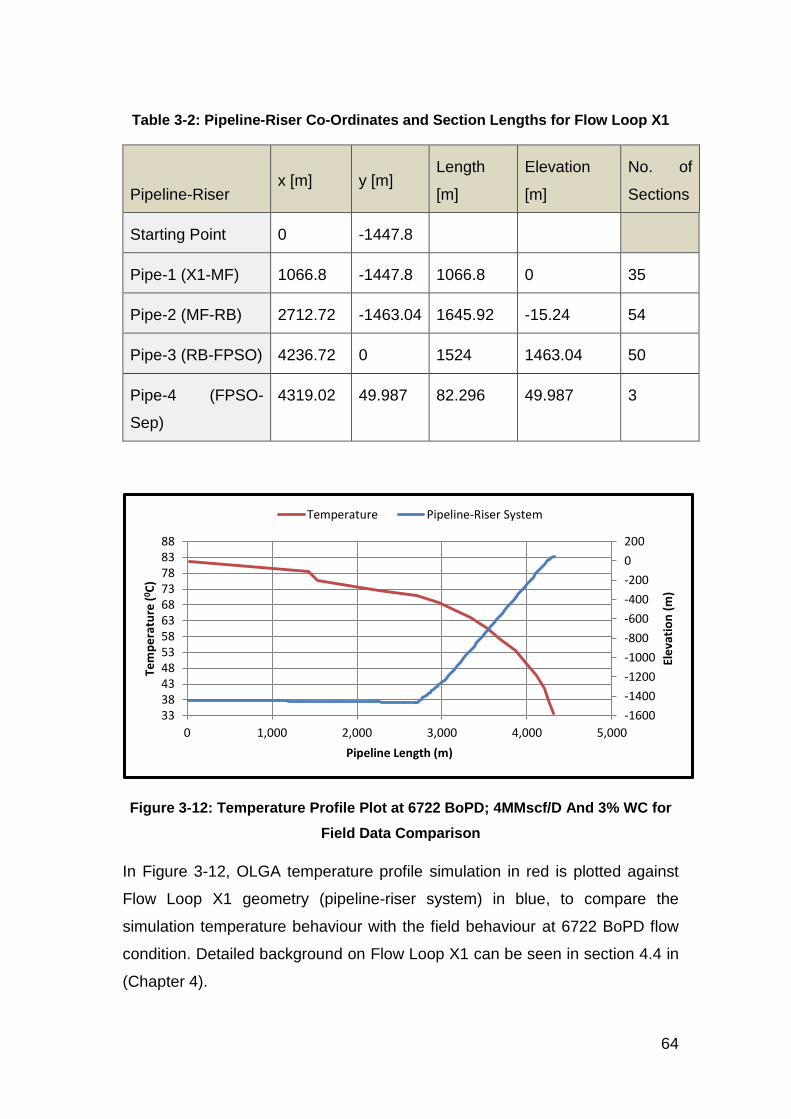
Figure 3-12: Temperature Profile Plot at 6722 BoPD; 4MMscf/D And 3% WC for Field Data Comparison ............................................................................. 64

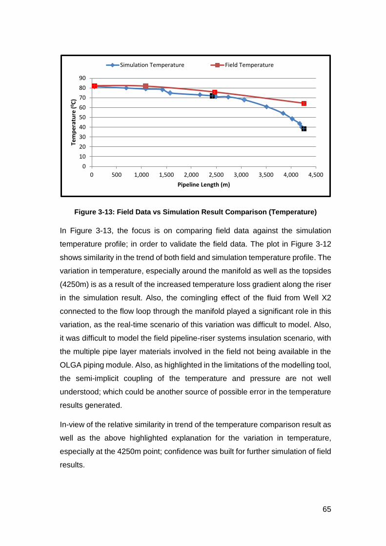
Figure 3-13: Field Data vs Simulation Result Comparison (Temperature) ....... 65

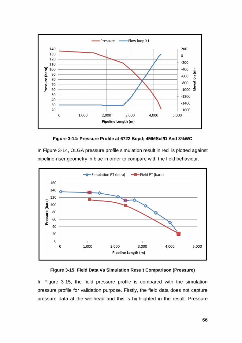
Figure 3-14: Pressure Profile at 6722 Bopd; 4MMScf/D And 3%WC ............... 66

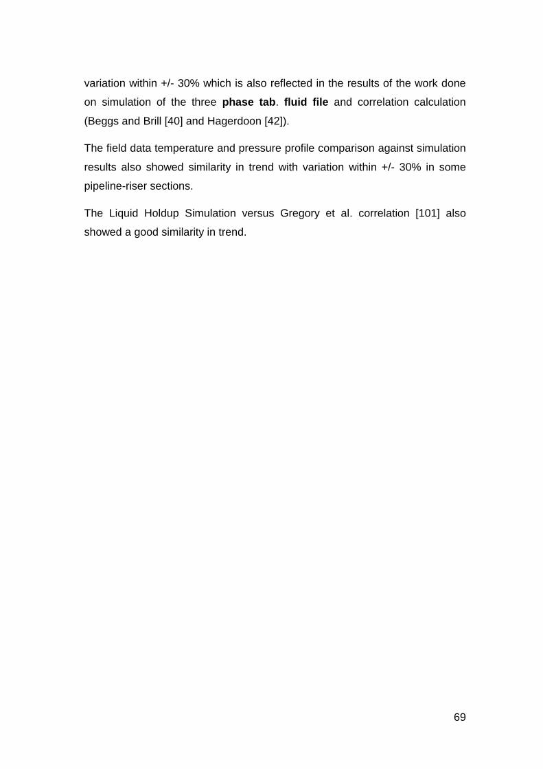
Figure 3-15: Field Data Vs Simulation Result Comparison (Pressure) ............. 66

Figure 3-16: Flow Chart of Study on Self-Lift Concept ..................................... 67

Figure 4-1: Egina North Loop without Control Measure (Geometry) ................ 75

Figure 4-2: Egina North Loop Gas Lift Case (Geometry) ................................. 76

Figure 4-3: Case with Topside Choking Visual GUL Display (Geometry) ......... 77

Figure 4-4: QLT Trend Comparison at Topsides (Pipe Section 7.5 - Topsides) 78

Figure 4-5: QLT Trend Comparison at Pipe Section 5.1 – (Riser Tower) ......... 79

Figure 4-6: Holdup Trend Comparison at Pipe Section 7.5 – (Topsides) ......... 80

Figure 4-7: Holdup Trend Comparison at Pipe Section 5.1 – (Riser Tower) .... 81

Figure 4-8: ID For Without Control Pipe Section 7.5 – (Topsides) .................... 81

Figure 4-9: ID for Pipe Section 5.1 without Control .......................................... 82

Figure 4-10: ID Profile Plot with Gas Lift .......................................................... 82

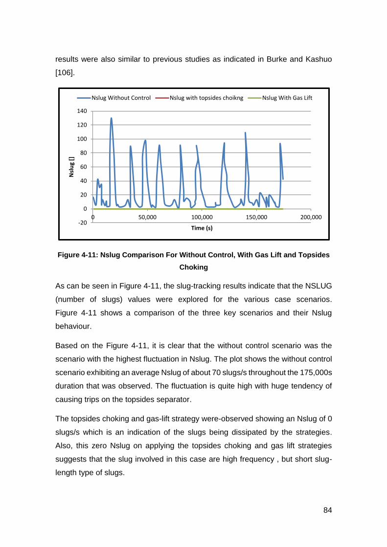
Figure 4-11: Nslug Comparison For Without Control, With Gas Lift and Topsides Choking ..................................................................................................... 84

Figure 4-12: Flow Regime ID Profile Plot vs Geometry At 6722 Bopd; 4 MMscf/D and 3%WC ................................................................................................ 88

Figure 4-13: Holdup Profile At 6722bopd, 4mmscf/D and 3%WC .................... 88

Figure 4-14: Flow Loop X1: Hydrodynamic Slugging Scenario ........................ 89

Figure 4-15: Hol Profile Plot vs Geometry ........................................................ 90

Figure 4-16: ID Profile vs Geometry At 10% WC .............................................. 91

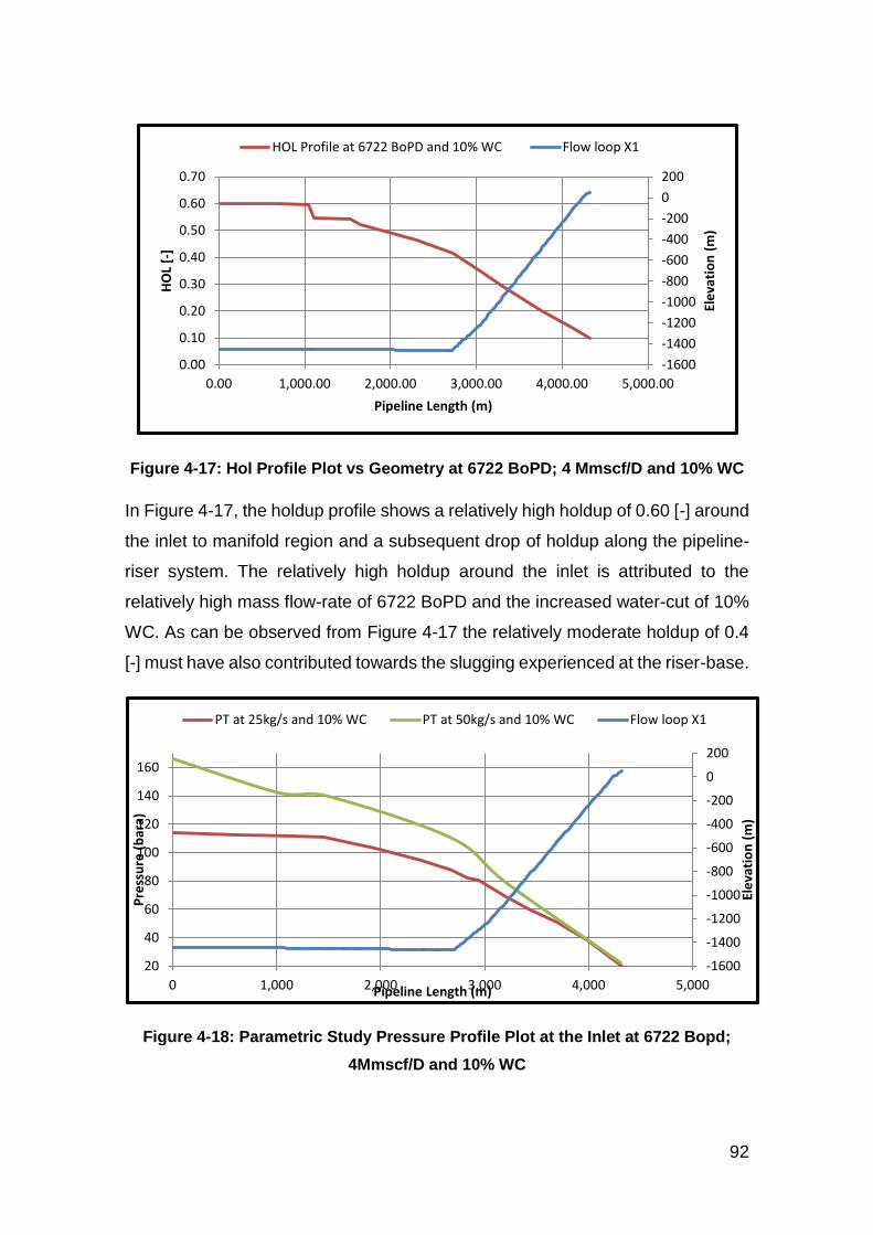
Figure 4-17: Hol Profile Plot vs Geometry at 6722 BoPD; 4 Mmscf/D and 10% WC ............................................................................................................ 92

Figure 4-18: Parametric Study Pressure Profile Plot at the Inlet at 6722 Bopd; 4Mmscf/D and 10% WC ............................................................................ 92

Figure 4-19: Parametric Study on ID Profile Plot at 6722 Bopd; 4mmscf/D and 10% WC .................................................................................................... 93

xiv

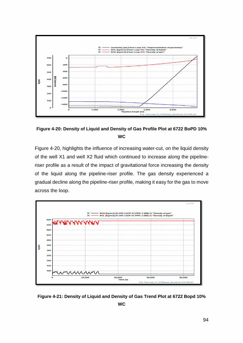
Figure 4-20: Density of Liquid and Density of Gas Profile Plot at 6722 BoPD 10% WC ............................................................................................................ 94

Figure 4-21: Density of Liquid and Density of Gas Trend Plot at 6722 Bopd 10% WC ............................................................................................................ 94

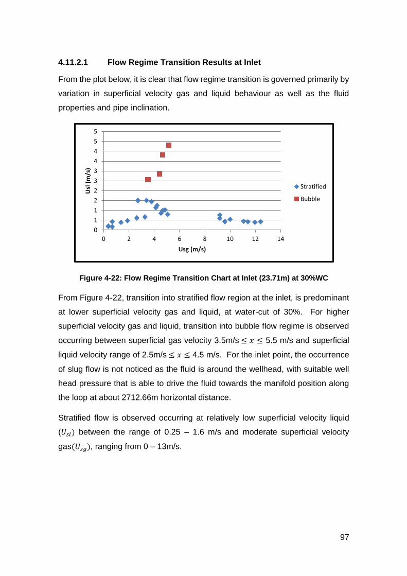
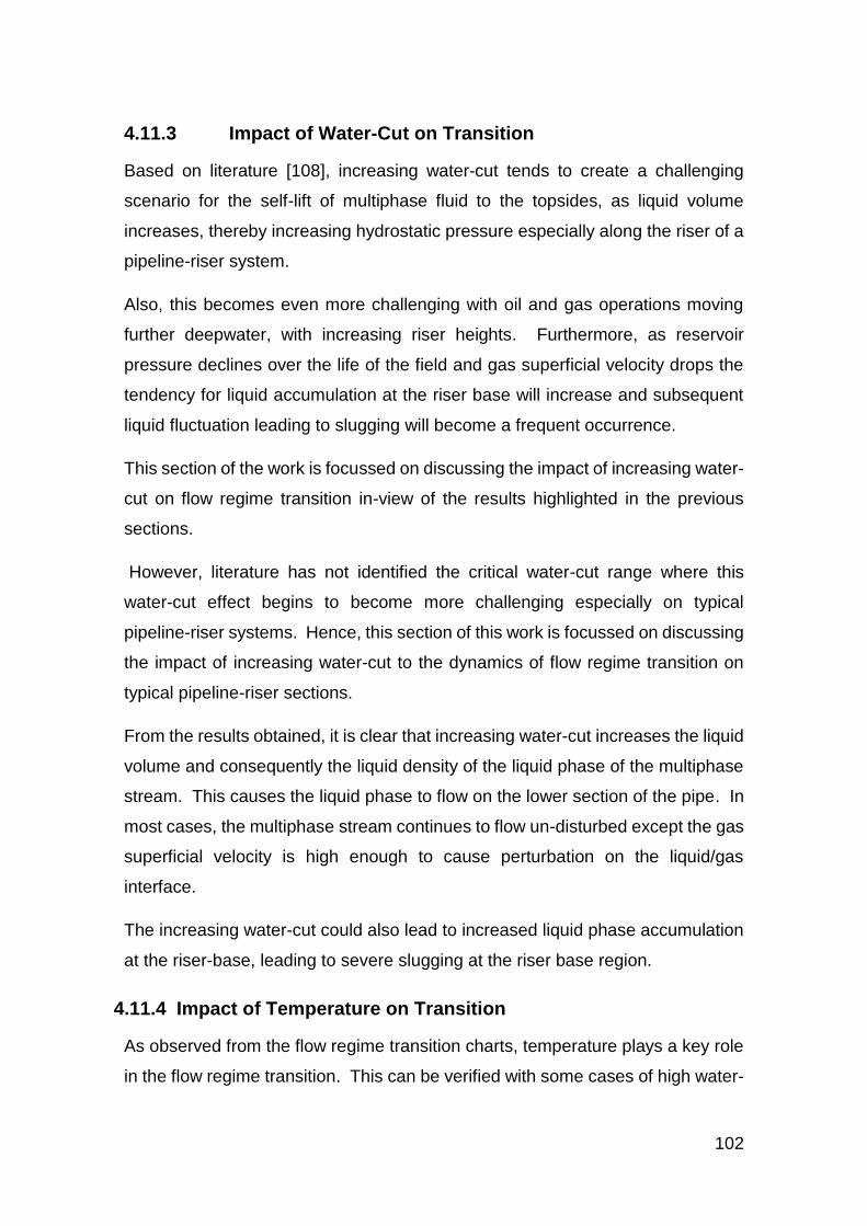
Figure 4-22: Flow Regime Transition Chart at Inlet (23.71m) at 30%WC ......... 97

Figure 4-23: Flow Regime Transition Chart at Inlet (23.71m) at 40% WC ........ 98

Figure 4-24: Flow Regime Transition Chart at MF (1066.8m) at 30% WC ....... 99

Figure 4-25: Flow Regime Transition Chart at MF (1066.8m) at 40% WC ....... 99

Figure 4-26: Flow Regime Transition Chart at RB (2712.72m) at 30% WC ... 100

Figure 4-27: Flow Regime Transition Chart at RB (2712.72m) at 40% WC ... 101

Figure 5-1: Schematic Diagram of Novel Approach: Self-Lift Approach (United States Patent No. 5478504), [104] ......................................................... 105

Figure 5-2: Numerical Model of Experiment (Geometry of Exp-1) .................. 106

Figure 5-3: Validation of Numerical Model with Experimental Data ................ 109

Figure 5-4: Experimental Data: Mesh Convergence of Numerical Model ....... 110

Figure 5-5: Experimental Self-Lift Model: Riser Base and Riser Top Pressure Trend ....................................................................................................... 110

Figure 5-6:Self-Lift Model: Experimental Liquid Hold-Up Trend at Riser Base 111

Figure 5-7: Experimental Self-Lift Model: Liquid Hold-Up Trend at By-Pass .. 112

Figure 5-8: Experimental Self-Lift Model: Gas & Liquid Flow Trend at Bypass ................................................................................................................ 113

Figure 5-9: Experimental Self-Lift Model: Flow Regime Trend at Bypass ...... 113

Figure 5-10: OLGA Self Lift Model (GUI): Field Data (Not Geometrically Accurate) ................................................................................................................ 116

Figure 5-11: Field Data Model: Severe Slugging ............................................ 118

Figure 5-12: Field Data Model: Number of Slugs in the Pipeline .................... 119

Figure 5-13: Field Data Model: Self-Lift with Severe Slugging ....................... 120

Figure 5-14: Field Data: Self-lift Total No. of Slugs in Pipeline ....................... 120

Figure 5-15: Field Data: Self-lift Manual Choke at Bypass ............................. 121

Figure 5-16: Field Data Pressure: Riser Base Gas-lift (RBGL) ....................... 122

Figure 5-17: Field Data: Self-lift Model with Gas Injection .............................. 124

Figure 6-1: Pressure Trend Convergence plot at (WH – MF) ......................... 126

xv

Figure 6-2: Temperature Trend Convergence plot at (WH – MF) ................... 126

Figure 6-3: Transient Plot of Well X1 Pressure at Varying Pipeline Section Length ................................................................................................................ 127

Figure 6-4: Plot of Production Pressure at Varying Pipeline Section Lengths 128

Figure 6-5: Pressure Trend at the Riser Base at Reducing Source 1 ............. 129

Figure 6-6: Liquid Holdup Profile Plots at Reduction Source 1 ....................... 130

Figure 6-7: Total Volumetric Flowrate Plot at Reduction in Source 1 ............. 131

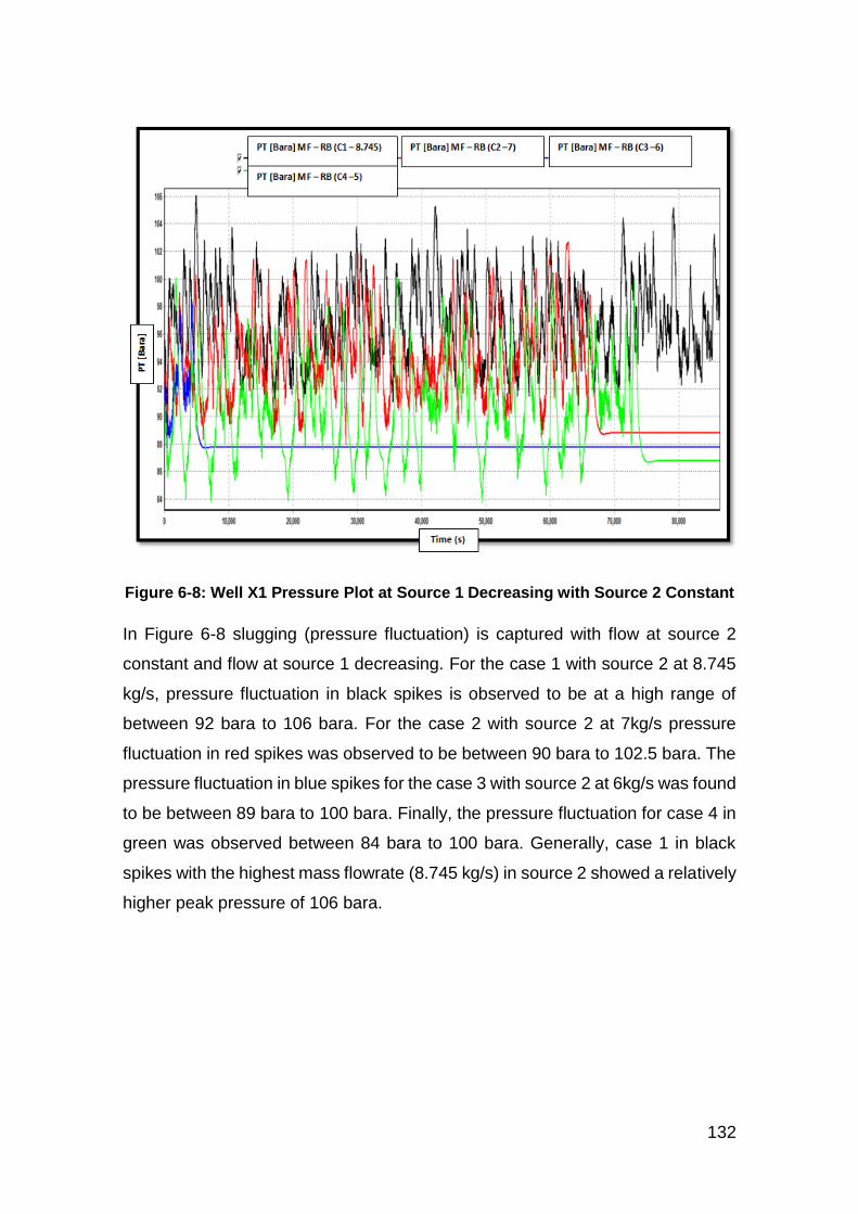
Figure 6-8: Well X1 Pressure Plot at Source 1 Decreasing with Source 2 Constant ................................................................................................................ 132

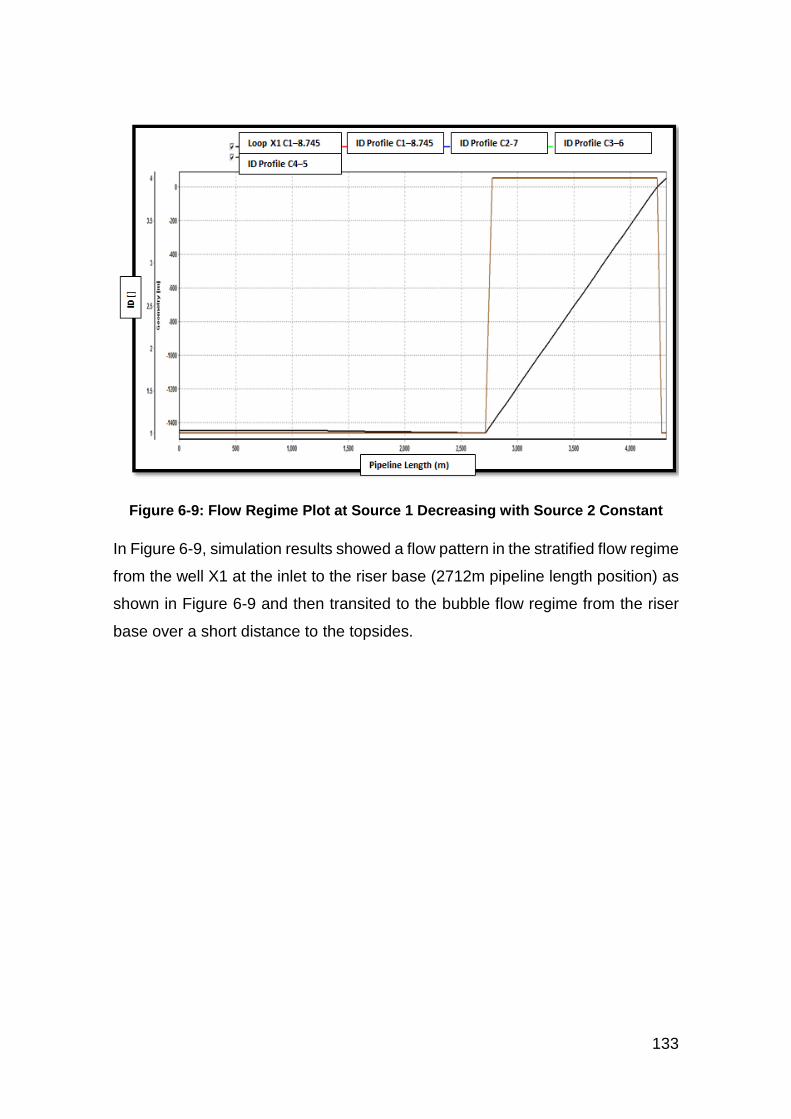
Figure 6-9: Flow Regime Plot at Source 1 Decreasing with Source 2 Constant ................................................................................................................ 133

Figure 6-10: Liquid Holdup Plot at Source 1 Decreasing with Source 2 Constant ................................................................................................................ 134

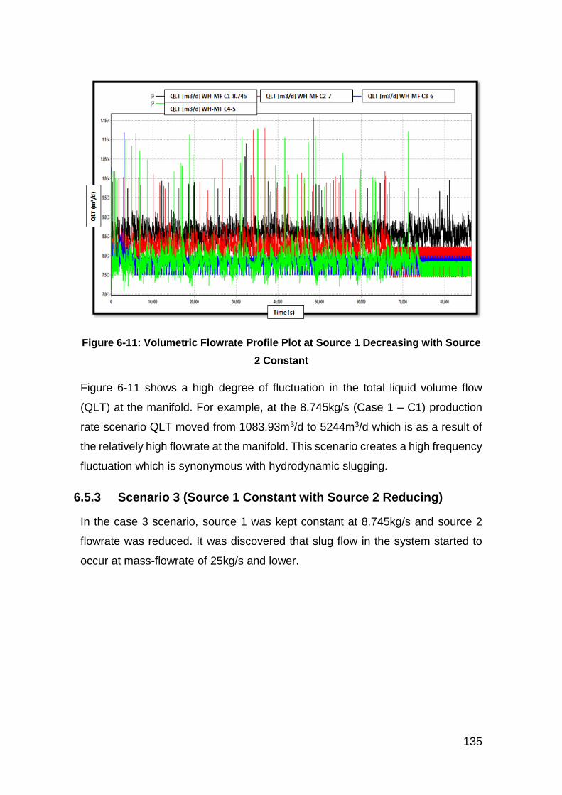
Figure 6-11: Volumetric Flowrate Profile Plot at Source 1 Decreasing with Source 2 Constant ............................................................................................... 135

Figure 6-12: WellX1 Pressure Plot at Source 1 Constant with Source 2 Reducing ................................................................................................................ 136

Figure 6-13: Plot of the Flow Regime at Source 1 Constant with Source 2 Reducing ................................................................................................. 137

Figure 6-14: Well X1 Pressure Plot at both Source 1 and Source 2 Reducing138

Figure 6-15: Total Volumetric Flow Rate Plot at both Source 1 and Source 2 Reducing ................................................................................................. 138

Figure 6-16: Slug Frequency of the Flow across the Pipeline- Riser System . 139

Figure 6-17: OLGA Model of the S3 (GUI) ...................................................... 140

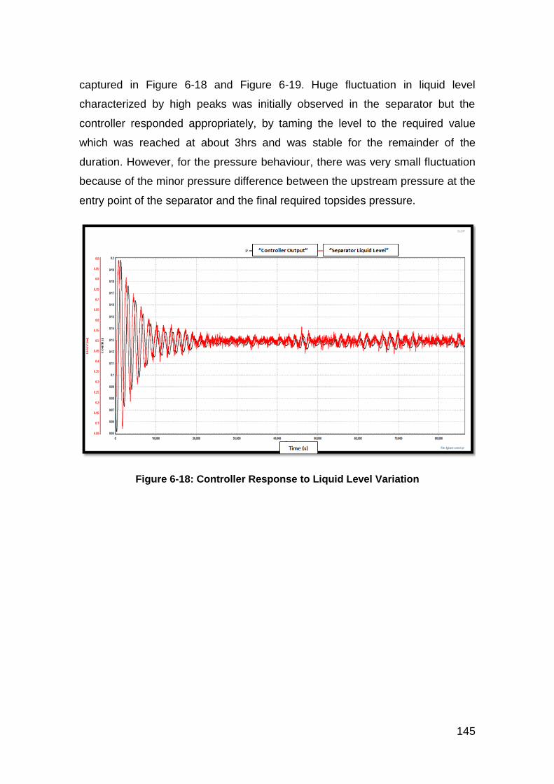
Figure 6-18: Controller Response to Liquid Level Variation ........................... 145

Figure 6-19: Controller Response to Pressure Variation ................................ 146

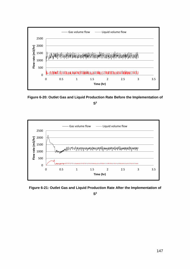
Figure 6-20: Outlet Gas and Liquid Production Rate Before the Implementation of S3 ........................................................................................................ 147

Figure 6-21: Outlet Gas and Liquid Production Rate After the Implementation of S3 ............................................................................................................ 147

Figure 6-22: Difference in Production Rate after the Implementation of S3 .... 148

Figure 6-23: Bifurcation Map for the Riser System ......................................... 149

Figure 6-24: Controller Behaviour: Riser-Base Pressure Control via Topside Choking ................................................................................................... 149

xvi

Figure 6-25: Liquid Production Rate for Topside Choking .............................. 150

Figure 7-1: M1 Diameter Effect Study Plot at MF on Flow Loop X1 ............... 152

Figure 7-2: M1 Diameter Effect Study Plot at RB on Flow Loop X1 ............... 152

Figure 7-3: M1 Diameter Effect Study Plot at TP on Flow Loop X1 ................ 153

Figure 7-4: M2 Diameter Effect Study Plot at MF on Flow Loop X1 ............... 154

Figure 7-5: ID Plot for M2 at 6” Pipeline-Riser Diameter ................................ 155

Figure 7-6: Pressure Trend at RB in the 2000m Case for 8" Pipeline-Riser System ................................................................................................................ 156

Figure 7-7: Pressure Trend at RB for the 2000m Case in the 10" Pipeline-Riser System .................................................................................................... 157

Figure 7-8: Pressure Trend at the RB for the 2000m Case for 12" Pipeline-Riser System .................................................................................................... 157

Figure 7-9: Pressure Trend at MF and RB for 3000m Depth in the 8" Pipeline-Riser System ........................................................................................... 158

Figure 7-10: Pressure Trend at MF and RB for 3000m Depth for 10" Pipeline-Riser System ........................................................................................... 159

Figure 7-11: Pressure Trend at RB for 3000m Depth in the 12" Pipeline-Riser System .................................................................................................... 159

Figure 10-1: OLGA Holdup Plot for Horizontal Pipeline .................................. 181

Figure 10-2: OLGA Pressure drop Plot for Horizontal Pipeline ...................... 183

Figure 10-3: Holdup for Pipe Inclined at Angle 40 degrees ............................ 186

Figure 10-4: Pressure Drop Plot for Pipe Inclined at Angle 40 degree ........... 188

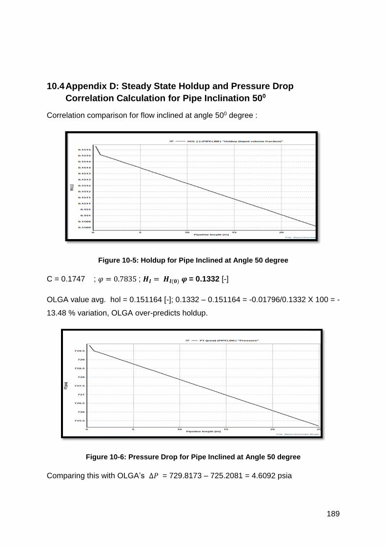
Figure 10-5: Holdup for Pipe Inclined at Angle 50 degree .............................. 189

Figure 10-6: Pressure Drop for Pipe Inclined at Angle 50 degree .................. 189

Figure 10-7: Holdup for Pipe Inclined at Angle 60 degree .............................. 191

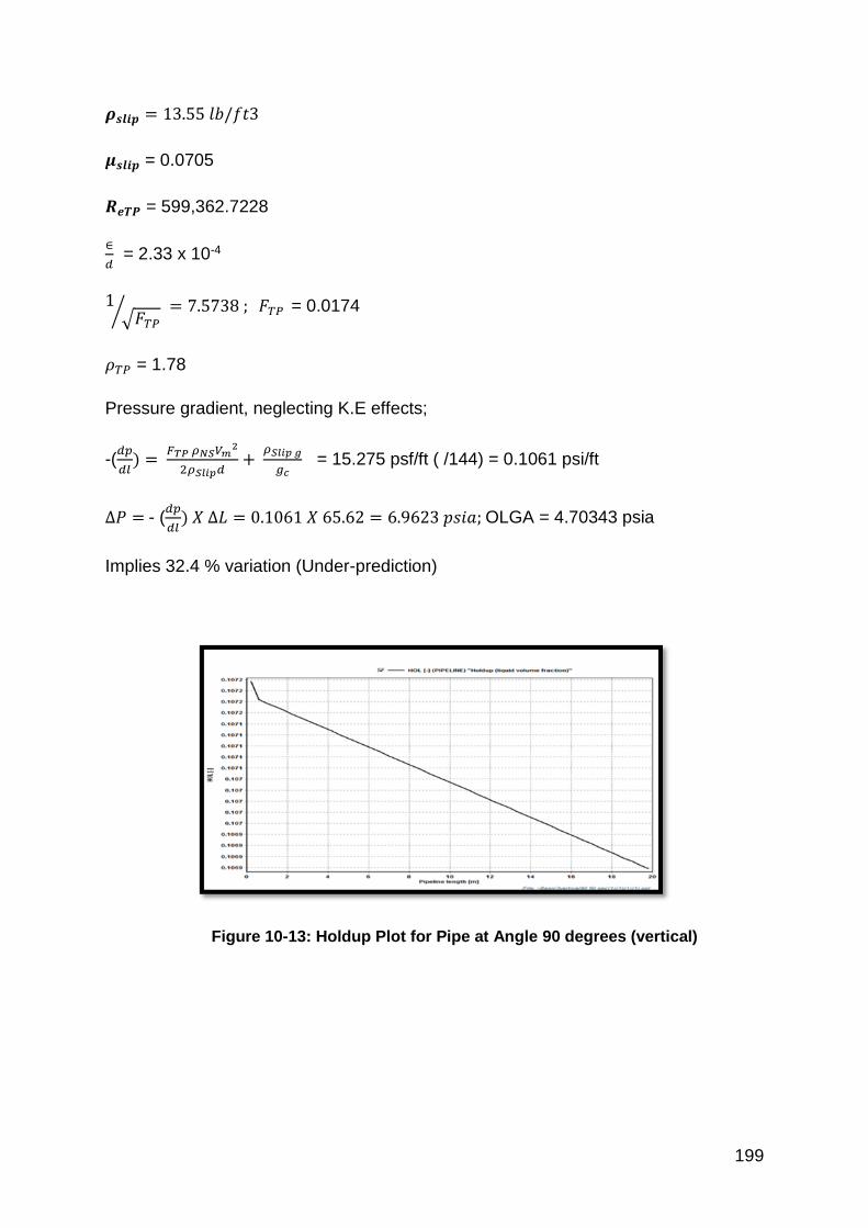
Figure 10-8: Pressure Drop for Pipe Inclined at Angle 60 degree .................. 191

Figure 10-9: Holdup for pipe inclined at Angle 70 degree .............................. 193

Figure 10-10: Pressure Drop for Pipe Inclined at Angle 70 degree ................ 193

Figure 10-11: Holdup for Pipe Inclined at Angle 80 degree ............................ 195

Figure 10-12: Pressure Drop for Pipe Inclined at Angle 80 degree ................ 195

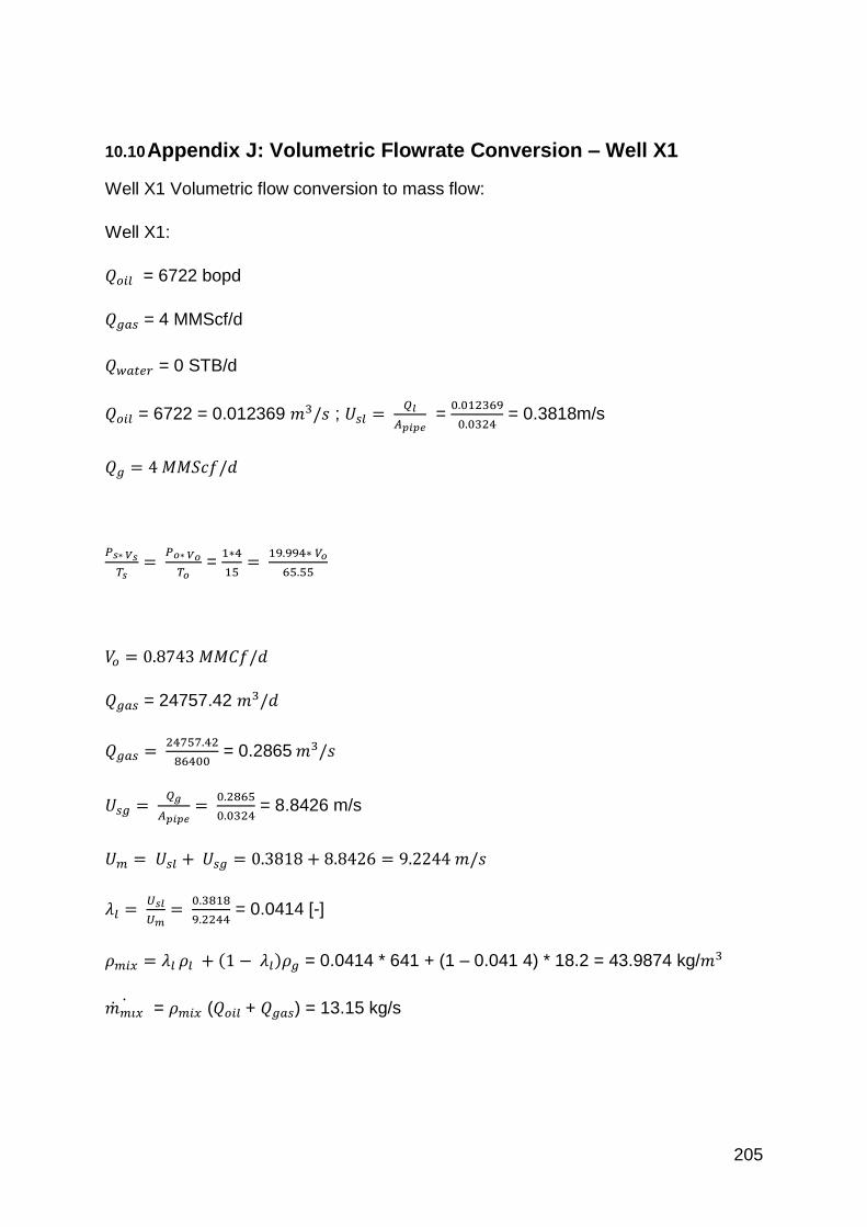
Figure 10-13: Holdup Plot for Pipe at Angle 90 degrees (vertical) .................. 199

Figure 10-14: Pressure Drop Plot for Pipe at Angle 90 degrees (vertical) ...... 200

xvii

Figure 10-15: Transient Pressure Profile at Angle 50 degree Convergence .. 201

Figure 10-16: Transient Holdup Profile at Angle 50 degree Convergence ..... 201

Figure 10-17: Transient pressure profile at Angle 60 degree Convergence ... 202

Figure 10-18: Holdup profile at Angle 60 degree Convergence...................... 202

Figure 10-19: Transient Pressure Profile at Angle 70 degree Convergence .. 203

Figure 10-20: Transient Holdup Profile at Angle 70 degree Convergence ..... 203

Figure 10-21: Pressure Profile at Angle 80 degree Convergence .................. 204

Figure 10-22: Holdup Profile at Angle 80 degree Convergence ..................... 204

Figure 10-23: Experimental Data Self-Lift Model: Riser Column Liquid Hold-up ................................................................................................................ 209

Figure 10-24: Experimental Data Self-Lift Model: Flow Regime Trend in the Riser Column .................................................................................................... 209

Figure 10-25: Flow Loop X1: Self-Lift Gas Re-injection Points ....................... 210

Figure 10-26: Flow Loop X1: 2% By-pass internal diameter sizing ................ 210

Figure 10-27: Flow Loop X1: By-pass Volume Flow Trend ............................ 211

Figure 10-28: Generic 2000m Pipeline-Riser System .................................... 214

Figure 10-29: Generic 3000m Pipeline-Riser System .................................... 214

Figure 10-30: Flow Regime Transition Chart at Inlet (23.71m) at 50% WC .... 220

Figure 10-31: Flow Regime Transition Chart at Inlet (23.71m) at 60% WC .... 220

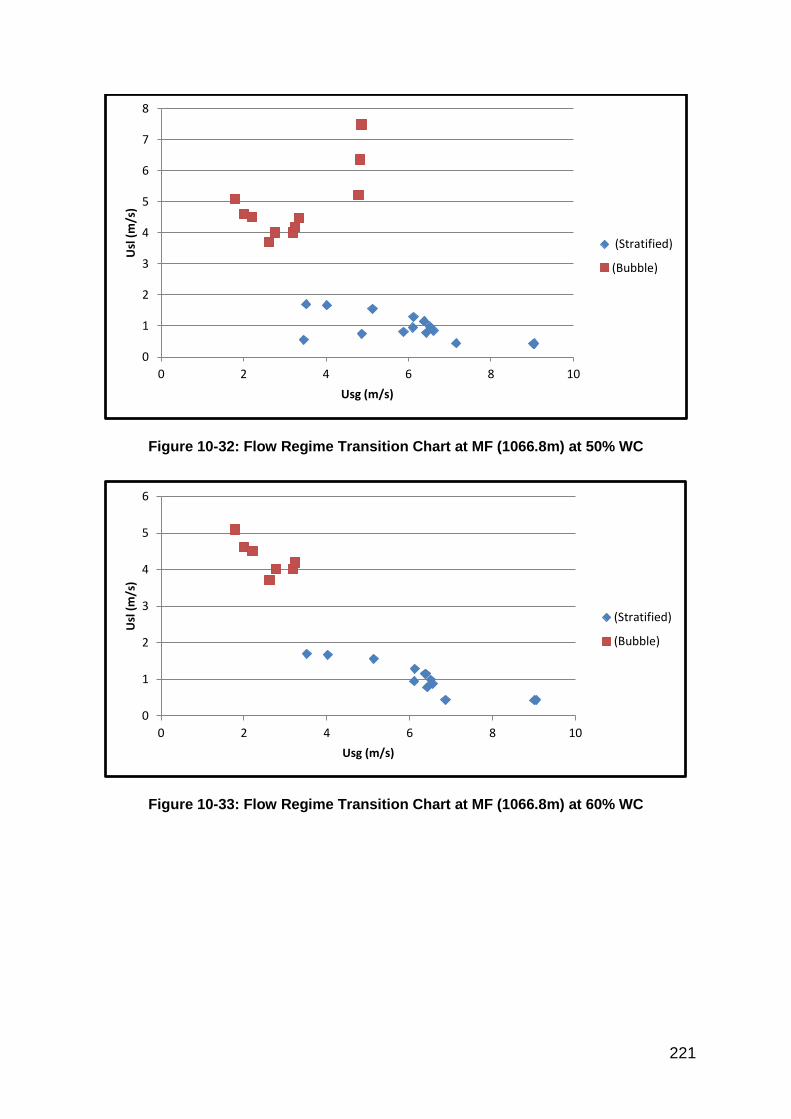
Figure 10-32: Flow Regime Transition Chart at MF (1066.8m) at 50% WC ... 221

Figure 10-33: Flow Regime Transition Chart at MF (1066.8m) at 60% WC ... 221

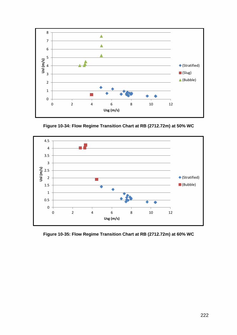
Figure 10-34: Flow Regime Transition Chart at RB (2712.72m) at 50% WC . 222

Figure 10-35: Flow Regime Transition Chart at RB (2712.72m) at 60% WC . 222

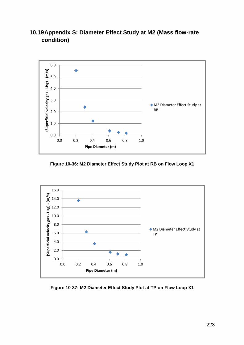
Figure 10-36: M2 Diameter Effect Study Plot at RB on Flow Loop X1 ........... 223

Figure 10-37: M2 Diameter Effect Study Plot at TP on Flow Loop X1 ............ 223

xviii

LIST OF TABLES

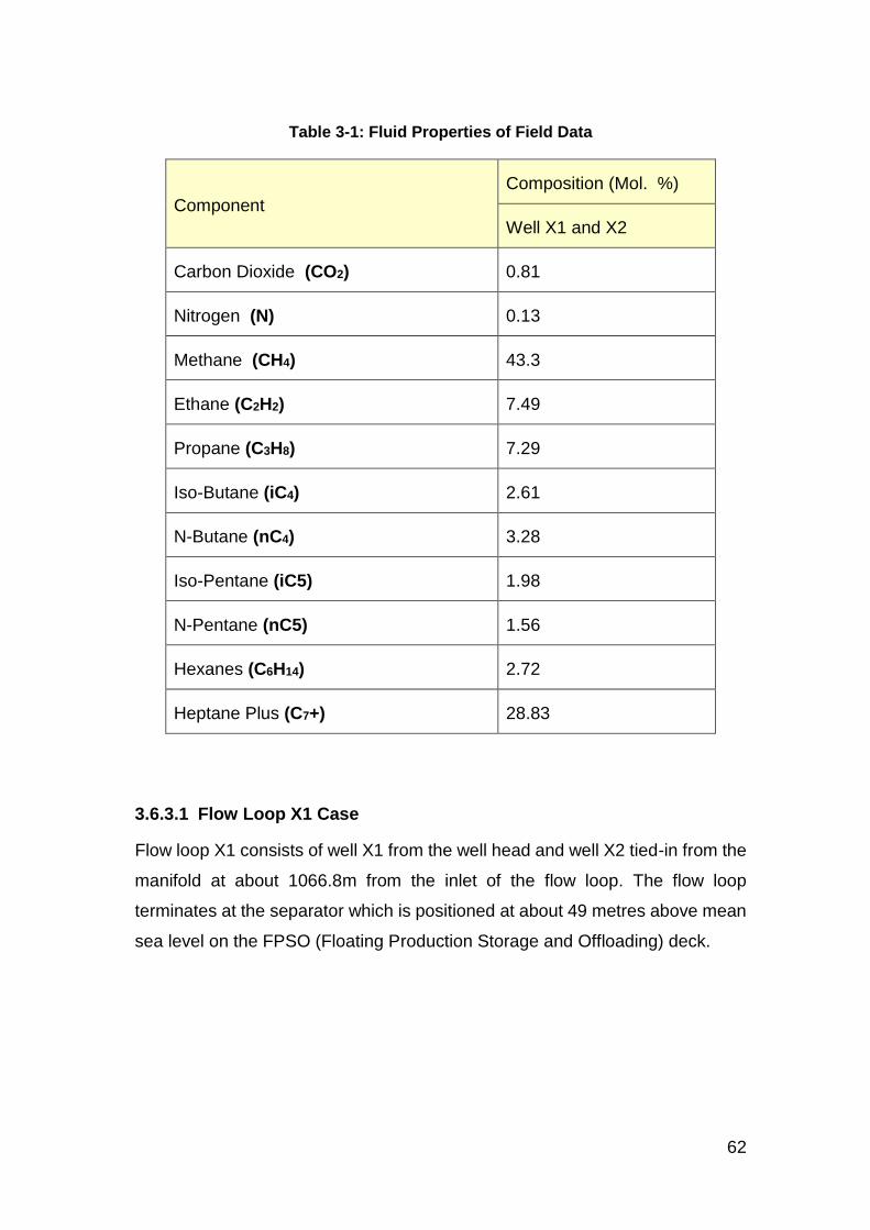
Table 3-1: Fluid Properties of Field Data .......................................................... 62

Table 3-2: Pipeline-Riser Co-Ordinates and Section Lengths for Flow Loop X1 .................................................................................................................. 64

Table 4-1: Egina Reservoir Fluid Composition as Adapted from [35], [105] ..... 73

Table 4-2: Egina Pipeline-Riser Geometry as Adapted from [35] ..................... 74

Table 4-3: Flow Geometry, Pressure and Temperature Readings at Core Loop Points ........................................................................................................ 85

Table 5-1: Pipe Coordinates and Section Lengths (Numerical Model-Experimental Data) ................................................................................. 107

Table 5-2 Pipe Positions and Section Lengths (Self-Lift Model of Experiment-1) ................................................................................................................ 108

Table 5-3: Flow Loop X1 Geometry, Pressure and Temperature ................... 114

Table 5-4: Pipe Positions and Section Lengths Numerical Model-Field Data) 115

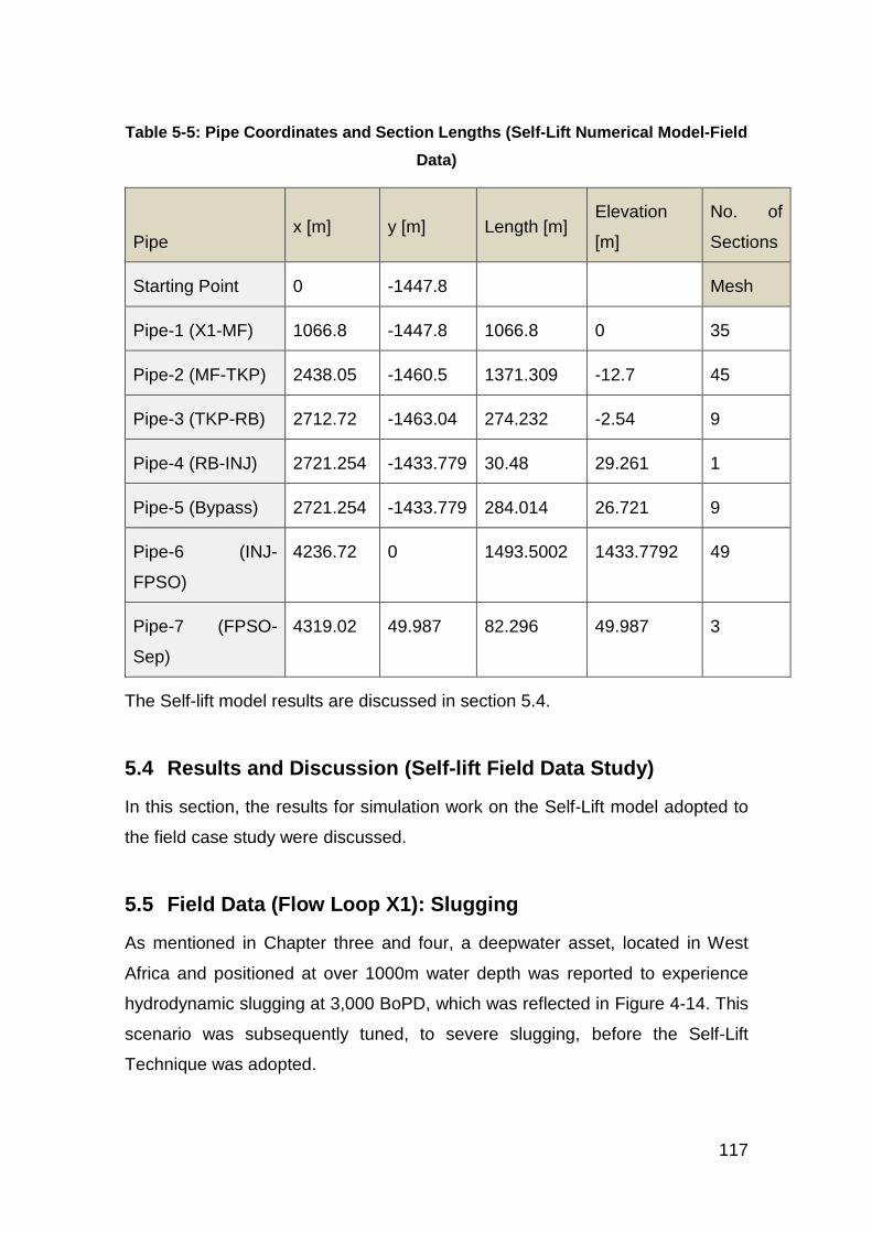
Table 5-5: Pipe Coordinates and Section Lengths (Self-Lift Numerical Model-Field Data) ............................................................................................... 117

Table 6-1: Separator Sizing and Weight Calculation of the S3 Unit for Flow Loop X1 In Comparison to the Otter and Penguins Project [113]. .................... 141

Table 6-2: Mini-Separator Vessel Construction Information (Aspentech 2003) ................................................................................................................ 141

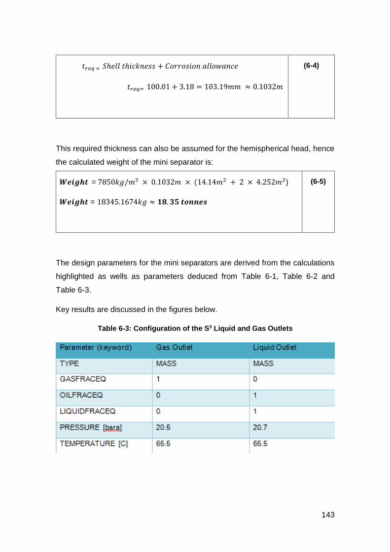
Table 6-3: Configuration of the S3 Liquid and Gas Outlets ............................. 143

xix

LIST OF ABBREVIATIONS AND GLOSSARY

BoPD Barrel of Oil Per Day

This is a measure of oil production per day

CAPEX CAPital Expenditure

This is a non-recurring expenditure invested on a project

DOTI Deep Offshore Technology International

This is an annual oil and gas industry conference with focus on deepwater assets

DPR Department of Petroleum Resources

A Nigerian government agency in charge of regulation the oil and gas industry in Nigeria

DWL Douglas Westwood Limited

A state of the art Global Energy Analysis Consulting firm

FEED Front End Engineering Design

A preliminary form of design carried out before detailed engineering design

FPSO Floating Production Storage and Offloading

A floating vessel or tanker for storing and offloading oil in deep offshore projects

GOR Gas Oil Ratio

The ratio of gas to oil in a multiphase fluid

GUI Graphical User Interface

A type of interface in a software that allows users to interact with the software through the available icons and visual indicators

HOL Liquid Holdup

A representation of the liquid volume fraction in a multiphase flow

HAMBIENT Ambient Heat Transfer

Coefficient of heat transfer within a particular system

ID Internal Diameter

The diameter of the inside of a pipeline-riser system

IFE Institute For Energy research

An Energy Research Institute based in Norway

IN INlet

The source of oil flow from an oil well

INJ INJection

A point along the flow loop for gas injection

xx

IPTC International Petroleum Technology Conference

An annual oil and gas conference focussed on new industry technology and knowledge sharing

KH Kelvin Helmhotz

Instability characterised by difference in velocity of two fluid phases flowing co-currently

MDC Marine Drilling Centre

A centre from which drilling is run on a set of wells

MF Manifold

A subsea structure containing valves and pipe-works designed to commingle and direct produced fluids from multiple wells into one or more flowlines

MMScf/d Million Standard cubic feet per day

An imperial measurement unit for gas

MRBL Multiphase Riser Base Lift

A slugging mitigation approach that involves diverting multiphase stream to a pipeline-riser system experiencing slugging

NSLUG Number of Slug

This is a trend parameter representing number of slugs formed per second

OLGA OiL and GAs

A commercial simulation tool for analysis of multiphase flow assurance issues

OPEX Operational Expenditure

This a recurring expenditure invested on a project

OTC Offshore Technology Conference

An annual oil and gas technology conference that holds at Texas, U.S.A

OVIP OLGA Verification and Improvement Project

A programme developed by industry for the verification of OLGA results and the general improvement of OLGA

PI Proportional Integral

A control feedback mechanism used in industrial control systems

PID Proportional Integral Derivative

A control loop system which attempts to minimize error over time by adjustment of a control variable

PLAC Pipeline Analysis Code

xxi

A numerical simulation code for multiphase flow analysis

ProFES Produced Fluid Engineering Software

A steady state and transient simulation tool for modelling slugging, hydrates, wax, corrosion and erosion issues

PT

Pressure reading

Instantaneous pressure reading at a particular point on the flowloop

PTDF Petroleum Technology Development Fund

A Nigerian government agency responsible for training and local man-power development for the oil and gas industry in Nigeria

PVT Pressure Volume Temperature

Key parameters reflected in the ideal gas law

QLT Total Liquid Volume Flow

This represents the total liquid volume flow profile plot after a simulation run in m3/s

RB Riser-Base

The base of the vertical riser

RBGL Riser Base Gas Lift

A technique for mitigation of severe slugging which requires injection of gas at the riser base

S3 Slug Suppression System

A technique for suppression of severe slugging which operates by control of liquid and gas volumes

SS1 Severe Slugging Type 1

A type of severe slug with liquid slug of riser length

SS3 Severe Slugging Type 3

A type of severe slug with slightly aerated liquid slug

STB/d Stock Tank Barrel per day

An imperial unit for measuring oil

STP Standard Temperature Pressure

The benchmark temperature and pressure used especially in running experiments

TAMBIENT Ambient Temperature

Temperature in a particular environment

TKP Take-Off-Point

The point along the flow loop from which compressed gas takes off in the Self-Lift Technique

xxii

TM Temperature reading

The instantaneous temperature reading at any part of a flow loop

TP ToPsides

The point where the multiphase fluid arrives on the FPSO

VKH Viscous Kelvin-Helmhotz

Instability at multiphase fluid interface influenced by fluid viscosity

VLW Viscous Long Wavelength

Long wavelength exhibited in fluids as a result of the fluid viscosity

WC Water-Cut

The percentage water fraction contained in the reservoir fluid

WH WellHead

The platform where the chokes and valves are situated for the control of fluid flow

xxiii

LIST OF SYMBOLS

Symbols Description Units

𝑨 Pipe cross-sectional area [ m2 ]

𝐴𝐺 Gas cross-sectional area [ m2 ]

𝐴𝐿 Liquid cross-sectional area [ m2 ]

𝐶 Courant number [-]

𝐹𝐷 Drag force [N/m3]

𝐹𝑅𝑀 Froude number [-]

𝐹𝑇𝑃 Friction factor [-]

𝑓𝑠 Slug frequency [Hz]

𝐺𝑔 Gas mass source [kg/s]

𝐺𝐿 Liquid mass source [kg/s]

𝐺𝐷 Liquid droplet mass source [kg/s]

𝒈𝒄 Gravity constant m/s2

𝐻𝐺 Gas hold-up [ - ]

𝐻𝐿 Liquid hold-up [ - ]

𝐻𝐿𝑠 Liquid holdup in slug area [ - ]

𝐻𝐵𝑠 Liquid holdup in bubble area [ - ]

𝑄𝐿 Liquid volumetric flow rate [ m3/s ]

𝑄𝐺 Gas volumetric flow rate [ m3/s ]

𝑅𝑒𝑁𝑆 Reynolds number [-]

𝑈𝑆 Slip velocity [ m/s ]

𝑈𝑆𝐿 Liquid superficial velocity [ m/s ]

𝑈𝐺 Gas linear velocity [ m/s ]

𝑈𝐿 Liquid linear velocity [ m/s ]

𝑈𝑀 Mixture velocity [ m/s ]

𝑈𝑆𝐺 Gas superficial velocity [ m/s ]

Vm Mixture velocity [m/s]

Vsg Gas superficial velocity [m/s]

Vsl Liquid superficial velocity [m/s]

𝑉𝑔 Volume fraction of gas [-]

𝑉𝐿 Volume fraction of Liquid [-]

xxiv

𝑣𝐿 Velocity of liquid [m/s]

𝑣𝑔 Velocity of gas [m/s]

𝑣𝑎 Velocity of air [m/s]

𝑣𝐷 Velocity of droplet [m/s]

𝑣𝑟 Relative velocity [m/s]

𝑉𝐷 Volume fraction of liquid droplets [-]

𝐿 Slug length [m]

𝑆𝐿 Wetted perimeter of liquid [m]

𝑆𝑖 Wetted perimeter of interface [m]

𝑆𝑔 Wetted perimeter of gas [m]

𝜆𝐿 Friction coefficient for liquid [-]

𝜆𝑔 Friction coefficient of gas [-]

𝜆𝑖 Friction coefficient of interface [-]

λl No slip holdup [-]

𝜌𝐺 Gas density [ kg/m3]

𝜌𝐿 Liquid density [ kg/m3]

𝜌𝑀𝐵𝑠 Mean gas bubble density [ kg/m3]

𝜌𝑀𝐿𝑆 Mean liquid slug density [ kg/m3]

𝜌𝑠𝑙𝑖𝑝 Slip density [kg/m3]

𝜓𝑔 Mass transfer rate between phases [-]

𝜓𝑒 Entrainment rate [-]

𝜓𝑑 Deposition rate [-]

ϴ Angle of inclination [ 0 ]

xxv

LIST OF EQUATIONS

(2-1) .................................................................................................................. 19

(2-2) .................................................................................................................. 19

(3-1) .................................................................................................................. 46

(3-2) .................................................................................................................. 46

(3-3) .................................................................................................................. 46

(3-4) .................................................................................................................. 47

(3-5) .................................................................................................................. 47

(3-6) .................................................................................................................. 47

(3-7) .................................................................................................................. 47

(3-8) .................................................................................................................. 48

(3-9) .................................................................................................................. 59

(6-1) ................................................................................................................ 141

(6-2) ................................................................................................................ 142

(6-3) ................................................................................................................ 142

(6-4) ................................................................................................................ 143

(6-5) ................................................................................................................ 143

(6-6) ................................................................................................................ 144

1

1 Introduction

In this chapter, the background of the research is captured, followed by the

motivation and the aim and objectives. Preliminary work on previous research is

set out together with some identifiable gaps in knowledge. The chapter ends with

a structure of the thesis.

1.1 Background and Motivation for the Study

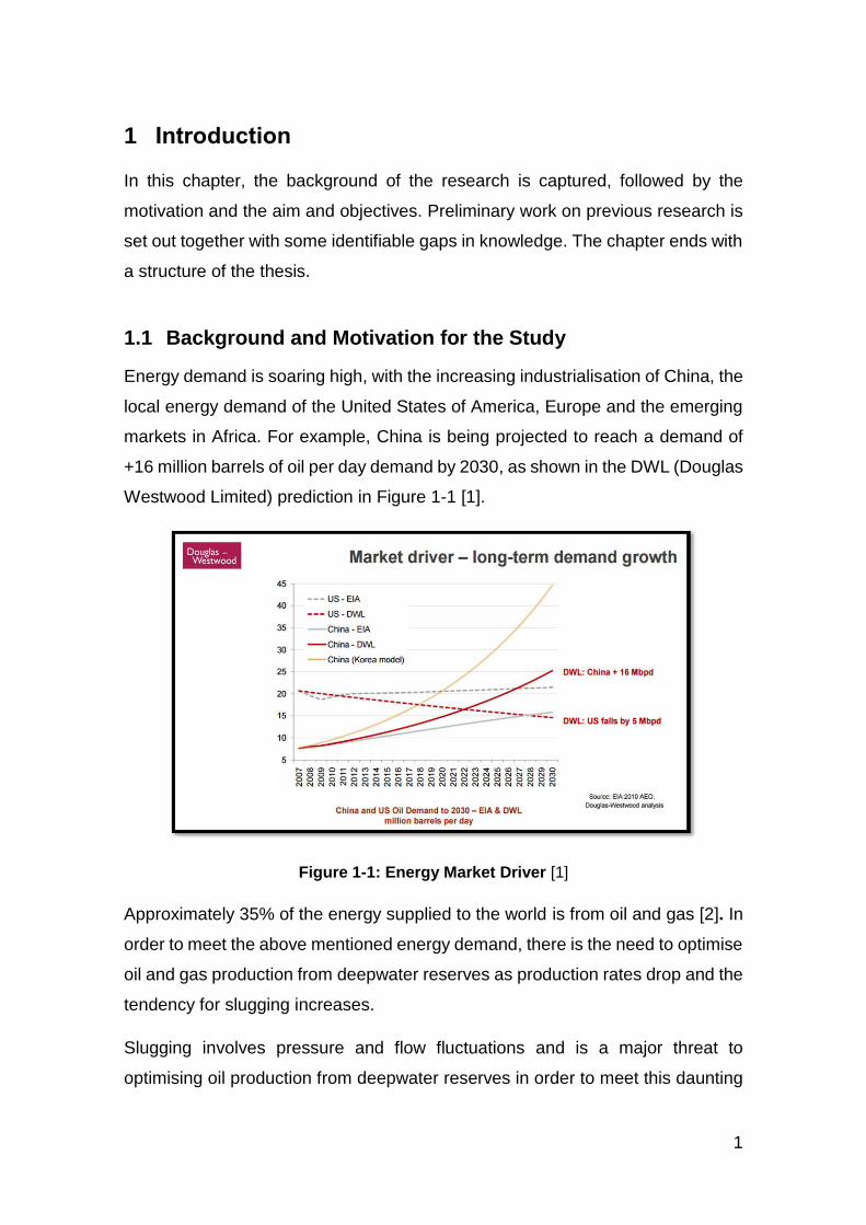
Energy demand is soaring high, with the increasing industrialisation of China, the

local energy demand of the United States of America, Europe and the emerging

markets in Africa. For example, China is being projected to reach a demand of

+16 million barrels of oil per day demand by 2030, as shown in the DWL (Douglas

Westwood Limited) prediction in Figure 1-1 [1].

Figure 1-1: Energy Market Driver [1]

Approximately 35% of the energy supplied to the world is from oil and gas [2]. In

order to meet the above mentioned energy demand, there is the need to optimise

oil and gas production from deepwater reserves as production rates drop and the

tendency for slugging increases.

Slugging involves pressure and flow fluctuations and is a major threat to

optimising oil production from deepwater reserves in order to meet this daunting

2

energy demand. Typical production loss from slugging can be as high as 50% as

highlighted in [3]. When this pressure fluctuation grows over the pipeline-riser

section, it causes trips on the valves and chokes on the separator, leading to a

shut-down of production. Also, the structural damage on pipeline-riser sections

as a result of slugging can cause huge economic loss to operators. Multiphase

flow transportation in deepwater pipeline-riser systems becomes more

challenging with complex piping networks and undulations that are common in

deepwater scenario, leading to increased liquid accumulation (liquid holdup) at

the low points. In-view of these inherent challenges, efforts are being made to

optimise oil recovery from deepwater reserves.

Also, in pipeline-riser design, one of the key issues considered is the proper sizing

of the pipeline-riser system to avoid slug flow. In order to achieve a suitable

design of pipeline-riser systems, industry has currently relied on flow regime

transition maps based on air-water experiments as highlighted in Mandhane et

al. [4] for Horizontal map and Barnea [5] for Vertical map. However, these maps

do not provide adequate basis for the design of pipeline-riser systems, as they

are based on air-water experiments done in mostly 2” and 4” pipeline-riser loops

as detailed in section 2.14. Hence, as part of this work, focus was on developing

a flow regime transition chart based on a sample deepwater case fluid package

with the intent of closely mimicking flow regime transition in a sample deepwater

pipeline-riser system and hence enhance pipeline-riser system design.

Fabre and Pere [6] defined severe slugging as the unstable behaviour of two-

phase flow encountered in oil production, associated with large amplitude

pressure fluctuation. It is also common to occur around the riser base and the

vertical section of the pipeline-riser system.

Hydrodynamic slugging is another type of slugging which occurs predominantly

along the horizontal pipelines. It is formed from stratified flow as a result of mainly

hydrodynamic wave instabilities between the liquid and gas phase [7].

Considering deepwater riser height sections and the capacity of gas to expand

as a result of very large hydrostatic pressures in deepwater scenario, there is the

tendency for severe slugging to become more critical in deepwater scenarios as

3

compared to shallow water scenarios. Hence, the design of facilities to be

installed at the platform becomes very crucial considering safety of operations

and the limited available space. Based on Hassanein and Fairhurst [8], typical

cost figures for the reliability failure is in the range of $30 to $50 million for typical

systems of 350.52 metres to 502.93 metres water depths. Projecting further from

this, sample failure of deepwater pipeline-riser systems as a result of structural

failures attributed to slugging is expected to be much higher and the remediation

efforts of any such reliability failures of subsea production facilities would also be

very expensive. The economic loss associated with drop in production as a result

of slugging is also a huge burden on operators.

In order to mitigate the production loss associated with slugging, researchers

have over the years investigated on mitigation strategies to handle slugging

problems. Some of the common industry strategies deployed include Topsides

Choking and Riser Base Gas Lift (RBGL) [8; 9]. However, the downside of

Topsides Choking for instance includes the reduction in production and the back-

pressure issues associated with Topsides Choking. In deploying Topsides

Choking, the valve opening is most times reduced in order to achieve flow stability

and this comes with economic loss, because production is drastically reduced.

Although, current research on how to stabilize flow at large valve opening is on-

going; however, the strategies are not yet robust for industry deployment. Also,

RBGL has its associated challenge regarding the compression of the gas to be

re-injected, as this comes with huge operational cost.

A key part of the research presented in this thesis focuses on how to improve

strategies for the prediction and mitigation of slugging problems in deepwater

pipeline-riser systems. Consideration will be given to sample upcoming

strategies; for example, Self-lift technique and S3 (Slug suppression system) in

order to test their viability in a deepwater scenario and explore how they can

utilised to cost-effectively mitigate slugging in deepwater scenarios.

4

1.2 Previous Research

In 1973, Yocum [3], reported that slugging has the potentials of reducing

production by 50%. Slugging is a phenomenon caused by the instabilities of water

and oil interface and the gas inertia effects in driving the oil out in an unsteady

manner [10]. The slugging phenomenon was recognised as a key flow assurance

issue, which deals with pressure and flowrate fluctuations in horizontal, slightly

inclined or vertical pipeline system. Slugging has been vastly researched;

however, one key challenge has been developing cost-effective solutions for

predicting and mitigating slug flow.

Until recently, the preferred solution has been to design the system such that

slugging potential is minimized or change the boundary condition by reducing the

topsides choke valve opening to eliminate slugging from the system [11]. None

of these solutions are optimal. Design changes often involve installation of

expensive equipment such as slug catchers and reducing the topsides choke

valve opening, which introduces pressure drop that impacts negatively on

production as reservoir pressure goes down putting a limit on oil production.

A different approach based on feedback control to mitigate riser slugging was

proposed by Schmidt et al. [12]. The main concept in that paper was to avoid

riser slugging by automatically adjusting the topsides choke valve position based

on an algorithm with a measurement of the pressure upstream of the riser and a

measurement of flow in the riser as inputs. Hedne and Linga [13] used a more

conventional PI (Proportional Integral) controller based on upstream pressure

measurement to avoid riser slugging. The studies of both Schmidt et al. and

Hedne and Linga are based on experimental works on medium scale loops and

they do show potential for using control solutions to mitigate slugging in

deepwater pipeline-riser systems. Also, both studies have not resulted in any

industrial application so far.

In the last fifteen years thereabout, some renewed interests have been observed

in control based solutions to avoid riser slugging. Courbout [14] presented a

control system to prevent riser slugging; implemented on Dunbar 16” flowline-

riser system. The approach of Courbout’s work was to implement control system

5

that utilizes the topsides choke valve to maintain the riser-base pressure at or

above the peak pressure in the slug cycle within the riser; thus preventing

accumulation of liquid at the riser base. This approach effectively removed riser

slugging in the system, but it performed by automating the old choking strategy,

rather that influencing the stability of the flow regimes within the pipe. Hence, an

extra pressure drop was introduced into the system due to high set-point for the

pressure controller. Henriot et al. [15] presented a simulation study for the same

pipeline as Courbout [14] where the setpoint for the riser base is considerably

lower. Kovalev et al. [16] reported that S3 was successfully implemented at some

shallow water fields (North Cormorant and Brent Charlie Platforms) at 150m and

140m depth respectively. Hence, part of this work was to review the S3 (Slug

Suppression System) and adapt it to the Flow Loop X1 (a sample deepwater field

flowloop with hydrodynamic slugging experience at 3000 BoPD) in deepwater

West Africa. The detail of adapting S3 to Flow Loop X1 is highlighted in Chapter

six (6).

Finally, Tangesdal et al. [17] proposed the Self-lift technique (slug mitigation

approach) which involves tapping off gas from the upstream pipeline system via

a by-pass pipe, into the riser column to mitigate slug flow by breaking the liquid

slugs within the riser column. This approach has been validated experimentally,

but no mention has been made in literature to adapting this strategy for mitigation

of slugging in sample deepwater oil fields. Hence, this also forms part of the

rational for this current work.

Generally, the thrust of the research presented in this thesis is on gaining a

clearer understanding of the conditions that initiate slugging in typical deepwater

oil field scenario (pipeline-riser systems) and developing strategies for predicting

as well as mitigating slug flow in typical deepwater scenarios (pipeline-riser

systems).

1.3 Gap in Knowledge

Analysis of slugging problems has hitherto focussed on managing the liquid

volumes arriving at the topsides. However, in-view of recent experience from

6

Gulf-of-Mexico the interaction between the gas bubbles behind the liquid slugs

are more problematic [18].

Drawing from the above background, this research is focussed on gaining an in-

depth understanding of the interaction between liquid and gas phase during

slugging initiation, growth and decay in deepwater scenario. This research is also

focussed on proposing cost-effective strategies for the prediction and mitigation

of slugging problems in deepwater pipeline-riser systems.

Some of the key parameters which were reviewed include;

Liquid Holdup

Gas Holdup

Pressure Drop

Mass Flowrate

Superficial Velocity Liquid (𝑈𝑠𝑙)

Superficial Velocity Gas (𝑈𝑠𝑔)

Key part of this research, involved developing a flow regime transition chart,

based on (𝑈𝑠𝑔 (𝑠𝑢𝑝𝑒𝑟𝑓𝑖𝑐𝑖𝑎𝑙 𝑣𝑒𝑙𝑜𝑐𝑖𝑡𝑦 𝑔𝑎𝑠) vs 𝑈𝑠𝑙 (𝑆𝑢𝑝𝑒𝑟𝑓𝑖𝑐𝑖𝑎𝑙 𝑣𝑒𝑙𝑜𝑐𝑖𝑡𝑦 𝑙𝑖𝑞𝑢𝑖𝑑)) as

well as considering the impact of field water-cut distribution; in order to ascertain

critical water-cut region at which slugging predominantly exits, which must be

avoided via suitable control/mitigation strategy.

The research presented in this thesis focusses on proffering a cost-effective

solution to slugging challenges in typical deepwater pipeline-riser systems using

the OLGA (OiL and GAs) numerical modelling tool.

1.4 Motivation of the research

Based on the impact of slugging (oil production loss) in the oil and gas industries,

experts and researchers have developed mitigating approaches to reduce

slugging thereby increasing oil production. However, there is need to improve

available mitigating strategies. This work therefore, focused on using the OLGA

(OiL and GAs) numerical modelling tool, to simulate typical deepwater cases with

7

slugging challenge in order to proffer cost-effective solution to slugging in

deepwater scenarios.

1.5 Research Aim and Objectives

The aim of this research was to understand, predict and mitigate slugging

problems in deepwater pipeline-riser systems. In order to achieve the aim, the

objectives for this research are as follows:

1. To conduct a review of flow regime, in-order to understand and predict

slugging envelope in typical deepwater fields.

2. To conduct a review on the conditions initiating slugging in deepwater

pipeline-riser systems.

3. Adapting of OLGA numerical model for analysis of slugging in typical

deepwater case studies.

4. Validation of numerical model against field data, published numerical and

experimental results.

5. Development of potential operational solutions for slugging prediction and

mitigation in deepwater pipeline-riser systems.

6. Demonstrating practical application of the developed solution, via software

and field applications.

1.6 Thesis Structure

This thesis offers a comprehensive analysis of flow assurance issues associated

with slugging in deepwater scenarios.

The scope of this thesis covers the following core areas as highlighted in the

summaries of the chapters below;

8

Chapter 1

This chapter provided highlights on the background of the study and definition of

fundamental concepts as well as the capturing of previous works done. Aim and

objectives were also defined.

Chapter 2

This chapter focusses on a fundamental review of the concept of flow assurance

and multiphase flow. An in-depth review of the slugging phenomenon was done.

Existing work on the process of slug formation, growth and decay was reviewed.

Slug prediction and mitigation were also critically reviewed and gaps in

knowledge identified which formed the basis of this work.

Chapter 3

Chapter three highlights the approach adapted for the study. Background on the

modelling tool was highlighted and validation of the modelling tool was done.

Justification for the approach adapted was done. Flowchart for the work was

developed.

Chapter 4

OLGA was adapted for the modelling of the Flow Loop X1 case. The model

adapted was validated against field data and sensitivity analysis was carried out

with respect to water-cut variation and mass flowrate variation.

Chapter 5

The Self-lift slugging mitigation strategy was adapted to Flow Loop X1 and the

results suggest that Self-Lift was only able to reduce riser-base pressure by

1.62%. Hence, it was recommended that Self-Lift be adapted on a case-specific

basis as it seems the pipeline inclination of Flow-Loop X1 impacted on the results

of adapting Self-Lift to Flow-Loop X1 and prevented gas from being tapped off

through the by-pass.

Reduction in by-pass size of the Self-lift technique improved the tendency of the

self-lift to mitigate slugging.

9

Chapter 6

The S3 (Slug suppression system) was defined and its principles clearly

highlighted. Convergence test was done in steady state and transient state to

build confidence in the prospective results. The S3 was then adapted to the Flow

Loop X1 case. One of the key results identified S3 as capable of 12.5% increase

in production.

Chapter 7

Firstly, this chapter reports that increasing riser depth increased the potential for

pressure fluctuation, considering the resultant increase in hydrostatic pressure.

Secondly, increasing pipeline-riser diameter had the tendency of generally

causing a drop in superficial gas velocity and consequently a drop in pressure

fluctuation. However, with a reported trend of a sudden increase in pressure from

10” to 12” pipeline-riser diameter case, it was clear that increase or decrease in

pressure fluctuation in a flowline-riser system was a function of a combination of

factors and not solely a function of directly proportional increase or reduction of

diameter of a pipeline-riser system.

Chapter 8

Principal findings of the research were mapped in this chapter, with explanation

on how the set of objectives were achieved, followed by contributions to

knowledge and implications of research. The chapter ends with limitations of

research and further work.

1.6.1 Publications

The following publications have so far resulted from this work;

Okereke, N.U. and Kara, F.; (DOTI – 2104, October, 2014), Numerical

Prediction of Slugging Problems in Pipes, proceedings of Deep Offshore

Technology International Conference, October 2014, Aberdeen, UK.

Okereke, N.U. et al. (IPTC – 2015), The Impact of increasing Depth and

Diameter on Flow regime Transition in Deepwater Flowlines and Risers,

10

International Petroleum Technology Conference (IPTC-18546-MS,

December 6-9, 2015, Doha Qatar) (In – View).

11

2 Literature Review

In this chapter of the research, focus is being placed on understanding of

multiphase flow, reviewing of existing works on slugging to understand how

slugs form, the various types of slugs and the mitigation approaches available

for handling slugging issues.

2.1 Background on Multiphase Flow and Flow Assurance

Considering work published on [19], multiphase flow in principle involves a flow

of liquids and gases occurring simultaneously. Multiphase flow is experienced

in our everyday life. For instance; rain (liquid phase) falling down through the air

(gas phase), or the bubble (gas phase) in our lemonade drink (liquid phase).

However, the focus of this work is on the multiphase flow that exists in oil, gas

and water in pipeline-riser systems [20].

Flow Assurance involves the engineering analysis of fluid properties, to develop

methodologies for solving multiphase flow production challenges such as

hydrates, asphaltene, wax and slugging [21]. The emphasis of this research is

on slugging and hence further review will be done on the concept of slugging.

2.2 Slugging

Slugging is basically a multiphase flow phenomenon in which liquid and gas

phase fluctuate at different superficial velocities, thereby leading to pressure

oscillations along the pipeline-riser system. Meglio et al. [22] defined slugging

as a two-phase flow regime occurring during the process of oil production. At

certain flow conditions, the inhomogeneous repartition of gas and liquid into the

long transport pipes leads to this oscillating flow pattern, which is detrimental to

the overall production. Based on Meglio et al. [22], the physical description of

the slugging phenomenon is as follows; Elongated bubbles of gas, separated

by “slugs” travelling from one end of a pipe to the other. This results in large

pressure oscillation and an intermittent flow. The main negative of slugging is

that the average (over time) production of oil is reduced compared to steady

12

flow regimes. Key types of slugging that will be reviewed include; severe

slugging and hydrodynamic slugging.

2.3 Severe Slugging

Fabre and Pere defined severe slugging as the unstable behaviour of two-phase

flow encountered in oil production [6]. Such situation corresponds to large

amplitude, long-duration instabilities which may reduce oil production and

damage installation. As part of his work, Schimdt et al. [23] highlighted that

severe slugging consists of four major steps: slug generation; slug production;

bubble penetration; and gas blowdown [12; 23]. The four steps are reviewed in

detail in sections 2.3.1 to 2.3.4.

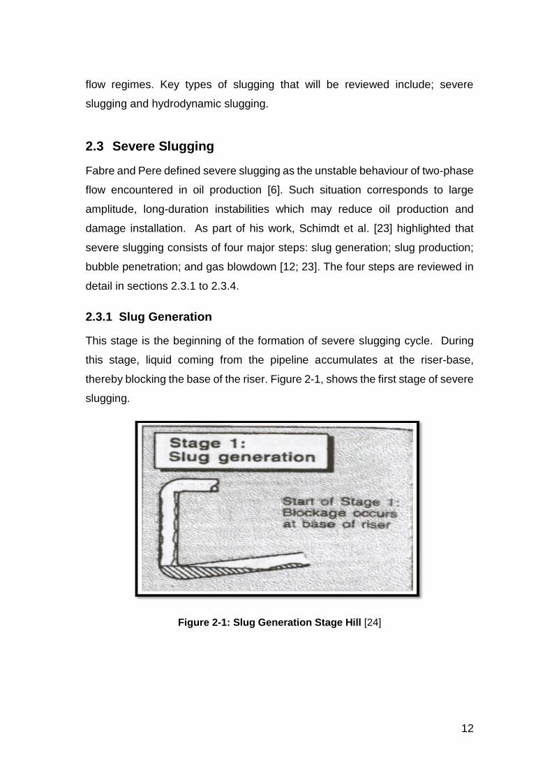
2.3.1 Slug Generation

This stage is the beginning of the formation of severe slugging cycle. During

this stage, liquid coming from the pipeline accumulates at the riser-base,

thereby blocking the base of the riser. Figure 2-1, shows the first stage of severe

slugging.

Figure 2-1: Slug Generation Stage Hill [24]

13

2.3.2 Slug Production

This is the second stage of severe slugging formation, in which the liquid level

within the riser increases and the liquid slug arrives at the topsides. As the gas

passage is blocked, the pressure in the flow line increases. The riser pressure

is also at its maximum value and also remains constant and the gas in the

pipeline tends to push the liquid into the separator. When the liquid arrives at

the riser-top, there will be a period of relatively steady production and the

hydrostatic pressure at the base of the riser would also remain constant. This

second stage is shown in Figure 2-2 below.

Figure 2-2: Slug Production Stage Hill [24]

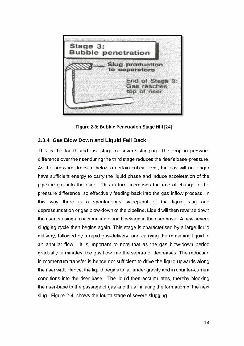
2.3.3 Bubble Penetration

The third step begins when the in-coming gas pushes the gas/liquid interface in

the flowline towards the base of the riser and the gas starts to penetrate the

riser. When the gas/liquid interface arrives at the riser-base, the gas continues

pushing the liquid into the riser proper, as shown in Figure 2-3. A series of

bubbles are formed and accelerate along the riser. The bubbles then displace

further liquid from the riser, expanding and thus reducing the pressure difference

over the riser.

14

Figure 2-3: Bubble Penetration Stage Hill [24]

2.3.4 Gas Blow Down and Liquid Fall Back

This is the fourth and last stage of severe slugging. The drop in pressure

difference over the riser during the third stage reduces the riser’s base-pressure.

As the pressure drops to below a certain critical level, the gas will no longer

have sufficient energy to carry the liquid phase and induce acceleration of the

pipeline gas into the riser. This in turn, increases the rate of change in the

pressure difference, so effectively feeding back into the gas inflow process. In

this way there is a spontaneous sweep-out of the liquid slug and

depressurisation or gas blow-down of the pipeline. Liquid will then reverse down

the riser causing an accumulation and blockage at the riser base. A new severe

slugging cycle then begins again. This stage is characterised by a large liquid

delivery, followed by a rapid gas-delivery, and carrying the remaining liquid in

an annular flow. It is important to note that as the gas blow-down period

gradually terminates, the gas flow into the separator decreases. The reduction

in momentum transfer is hence not sufficient to drive the liquid upwards along

the riser wall. Hence, the liquid begins to fall under gravity and in counter-current

conditions into the riser base. The liquid then accumulates, thereby blocking

the riser-base to the passage of gas and thus initiating the formation of the next

slug. Figure 2-4, shows the fourth stage of severe slugging.

15

Figure 2-4: Gas Blow-Down Stage Hill [24]

Yocum [3] and Taitel [25] also reported of the slugging steps to confirm the

behaviour earlier highlighted. Schimdt in [26] undertook an extensive

investigation of the experimental behaviour of pipeline/riser systems. He also

proposed the first model requiring an empirical correlation to calculate liquid fall

back. Schmidt et al. in [23] later improved on the physical model by generating

four different equations for slug generation, slug production, bubble penetration

and gas blow down. Their results were in good agreement with downward

sloping pipe; however the model could not probably cover the full cycle for

horizontal pipe.

Further work by Pots et al. [27] discussed how to scale a laboratory flow loop to

simulate the behaviour of field installation. They mentioned the occurrence of

slugging at low liquid flow rates but suggested flowline undulations as the cause.

This thesis focuses its review predominantly on severe slugging and

hydrodynamic slugging.

2.4 Hydrodynamic Slugging

Hydrodynamic slugging occurs mainly in the horizontal section of a typical

pipeline-riser system. It is generated from stratified flow as a result of growth in

hydrodynamic wave instabilities between gas-liquid interface and gravitational

16

force imbalance between gas and liquid phase generated by change in

geometry [7]. It has been highlighted that the development of hydrodynamic

wave instabilities depends on classical Kelvin Helmholtz instability mechanism

[28], [29], [30]. The effects of wave behaviour on the formation of hydrodynamic

slugs in two-phase flow at relatively low gas and liquid velocities, was studied

by Arnaud et al. [31]. Their experiment was carried out on a 10cm internal

diameter pipe, which was 31m long and positioned horizontally. Key part of their

discovery was that formation of hydrodynamic slugs as a result of wave

interaction was different from predictions of formation of slugs based on long

wavelength stability theory.

Research on hydrodynamic slug flow has resulted in the development of a

number of transient and steady state models. Issa and Kempf [7], suggested

classification of the transient models into three categories, namely: empirical

slug specification; slug tracking; and slug capturing. Empirical slug specification

models are deployed to highlight various key stages of slug development;

including slug initiation, growth and decay [25], the slug tracking models are

used to track the movement, growth and dissipation of individual slugs in slug

flow [32]. A slug tracking technique with capacity to predict slug initiation, growth

and dissipation was also developed by Zheng et al. [33]. The capturing models

are designed to predict hydrodynamic slug flow based on mechanistic and

automatic results of hydrodynamic growth instabilities [34].

2.5 Slug Flow Characteristics

Key parameters that influence slug flow behaviour were reviewed in this section

of the work.

2.5.1 Liquid Holdup

The area fraction or volume fraction occupied by the liquid phase within a two-

phase gas-liquid flow is known as liquid holdup. If for instance, the gas volume

fraction ∝𝑔 = 0.25, then the liquid volume fraction is ∝𝑙 = 1 – 0.25 = 0.75. This

implies that the liquid volume fraction occupies three quarter of the pipe section,

17

while the gas volume fraction occupies one quarter of the pipe section. In slug

flow, the liquid holdup is the liquid volume fraction [19; 35]. Research has shown

that the slug liquid holdup is majorly influenced by gas and liquid flow rates, the

fluid properties and inclination angle of the pipe [36; 37].

Research has shown that liquid holdup behaviour is also majorly influenced by

the liquid film ahead of the liquid slug being scooped up and a new film forming

in its wake [38]; [39]. Also, literature reports that there is some gas entrainments

observed within the slug in the process of this scooping action [38], [39].

2.5.2 Gas Holdup

The area fraction or volume fraction occupied by the gas phase within a two-

phase gas-liquid flow is known as gas holdup. If for instance, the gas volume

fraction ∝𝑔 = 0.75, then the liquid volume fraction is ∝𝑙 = 1 – 0.75 = 0.25. This

implies that the gas volume fraction occupies three quarter of the pipe section,

while the liquid volume fraction occupies one quarter of the pipe section. In slug

flow, the gas holdup is the gas volume fraction [19; 35].

2.5.3 Pressure Drop

Pressure drop is a measure of the pressure differential along the pipeline-riser

system, as the fluid flows from the pipeline-riser inlet to the topsides. It is

governed by Beggs and Brill [40; 41] correlation for the horizontal and slightly

horizontal pipeline and Hagerdoon [42] vertical pipeline correlation. The Beggs

and Brill [40; 41] correlation is reflected by three key components;

(a) Frictional pressure gradient

(b) Gravitational pressure gradient

(c) Acceleration pressure gradient.

(d) Total pressure gradient

These components sum up to give rise to the total pressure gradient. [40], [42]

, [43] and [4].

18

2.5.4 Slug Length

The slug length of a unit slug refers to the sum of the liquid slug length and the

gas bubble. Slug dissipation in the upward pipe inclination is suggested to be

related to length, angle and diameter of the pipe [35], [44].

2.5.5 Slug Frequency

The concept of slug frequency refers to the number of slugs passing across a

section of a pipeline over a specified period of time. It is a fundamental

parameter required in the analysis of fatigue in pipeline-riser systems. OLGA

delay constant is programmed to match by default to Shea correlation [45]. Shea

correlation is defined as 𝑓 = 0.68 𝑈𝑠𝑙

𝐷1.2𝐿0.6 where 𝑓 is slug frequency expressed in s-

1, 𝑈𝑠𝑙 is superficial velocity liquid expressed in (m/s), 𝐷 is pipeline diameter

expressed in metres and 𝐿 is the dimensionless slug length expressed in

number of Pipe D (diameter) [35], [46].

2.5.6 Slug Period

Slug period refers to the duration of slug existence over the life of a field. It is a

very critical parameter used in ascertaining the number of stress cycles to be

applied to riser-base spools [35].

2.5.7 Slug Velocity

Slug velocity refers to the speed at which a slug is being propagated. This speed

may be the same or faster than the speed at which bulk fluid is moving. It is an

important parameter for computing the impact of slug force on pipe bends as

fluid momentum change happens at pipe bends [35].

2.5.8 Slug Density

The density of a unit slug is another critical parameter. It is very relevant in

pipeline-riser fatigue analysis. The mean liquid and gas slug density are a

function of slug liquid and bubble hold-ups [35]. The mean liquid slug

density𝜌𝑀𝐿𝑠, is defined based on the slug holdup, the liquid and gas phase

densities and slug liquid hold-up 𝜌𝐿 , 𝜌𝐺, and 𝐻𝐿𝑠 respectively, as follows:

19

𝜌𝑀𝐿𝑆 = 𝜌𝐿 𝐻𝐿𝑠 + 𝜌𝐺 ( 1 − 𝐻𝐿𝑠) (2-1)

Similarly, the mean gas bubble density 𝜌𝑀𝐵𝑠 is defined based on liquid and gas

phase densities and liquid holdup in the bubble area 𝜌𝐿 , 𝜌𝐺, and 𝐻𝐵𝑆

respectively, as follows:

𝜌𝑀𝐵𝑠 = 𝜌𝐿 𝐻𝐵𝑆 + 𝜌𝐺 (1 − 𝐻𝐵𝑠)

(2-2)

2.6 Slug Flow Behaviour and Prediction

Based on work done by Yocum [3] the symptoms of severe slugging

phenomenon were first captured for typical oil and gas multiphase flow in

pipeline-riser systems. He observed that flow capacity could be reduced by 50%

due to backpressure fluctuations caused by severe slugging.

This backpressure fluctuation is a function of the negative pressure differential,

between the riser-base pressure and the topsides pressure as also highlighted

in the study of Ehinmowo [47]. The negative pressure fluctuation occurs as a

result of variation in gas and liquid superficial velocities; driven primarily by low

gas superficial velocity.

Schmidt in [12] reported that there was a significant difference between

hydrodynamic slugging and severe slugging as reported by Yocum in [3].

Schmidt in [26] made a proposal of flow regime maps for severe slugging based

on Duns and Ros dimensionless gas and liquid velocity numbers. Doty and Dale

in [48] developed a hydrodynamic model for predicting the dynamic slug

characteristics of severe slugging. The model assumed constant inlet liquid and

gas mass flowrates, constant separator pressure, and liquid slugs free of

entrained bubbles, and required empirical correlations for the liquid hold up in

the pipeline and the liquid fall back in the riser. The authors presented three

separate severe slugging transition criteria:

20

Stratified to non-stratified flow transition; i.e. they postulate that the flow

in the pipeline segment before the riser has to be stratified for severe

slugging to occur.

The stability of the flow in the riser, i.e. as gas flow rate increases, the

pressure drop in the riser decreases for a given liquid flowrate. Hence,

the flow is defined as unstable.

The criterion in allocating the boundary between severe slugging and

transition to severe slugging is a direct solution of their hydrodynamic

model for the lowest gas flowrate corresponding to a liquid flowrate that

will produce riser generated slugs shorter than the riser length.

Slugging as a phenomenon can occur within the horizontal, inclined or vertical

flexible or rigid riser section. For the inclined pipe section, the multiphase flow

content flowing upwards does tend to assist the initiation of slugging [49]. This

is illustrated in Figure 2-5:

Figure 2-5: Slug Flow Formation in an Inclined Pipe (Oil & Water Mixtures) [50]

From Figure 2-5, A-displays the fluctuation in the different phases; B-shows the

accumulation of the liquid phase at the lower elevation, leading to gas

entrainment; C-shows the generation of slug growth upwards into the riser

section.

Research by Shotbolt [51] confirms that slug flow influences three major areas

of concern:

21

“Arrival volume rate of the most severe liquid slug expected” and the

“differences between flowrates and pressures at the beginning and end

of the gas bubble flow”.

Suitable riser base pressures capable of stopping flowline flow.

“Momentum change reactions”, which is capable of causing vibrations

along the riser

An original study done by Schmidt et al. [12] grouped severe slugging into two

types: Severe Slugging with liquid slug flow of riser length and Severe Slugging

with slightly aerated liquid slugs that does not exceed typical riser height. Based

on Schmidt et al. [12], the first slug type can be eliminated by varying either flow

rate of the gas or flowrate of the liquid. With the second slug type, Schmidt et

al. [12], stated that; depending on the liquid flowrate, an increase in flowrate of

gas could lead to annular or slug flow. Malekzadeh et al. [52], succeeded in

classifying slugging into three types SS1, SS2 and SS3; based on the liquid

content of the slugs or how aerated the slugs are. Figure 2-6, captures the

description of the two key extremes (SS3 and SS1).

Figure 2-6: Types of Slugging As Grouped By Malekzadeh et al. [52]

22

In Figure 2-6; (a) Highlights Severe Slugging Type 3 (SS3) with more aerated

liquid slugs. Figure 2-6 (b) highlights a classic Severe Slugging Type 1(SS1)

with a “pure liquid slug” length.

2.7 Slugging Elimination

Yocum in [3] identified severe slug flow elimination techniques that are still

considered at the present time. These include; reduction in line diameter,

splitting of the flow into dual or multiple streams, gas injection at the riser-base,

the use of mixing devices at the riser-base, topsides choking and back-pressure

increase. Yocum [3] noticed that the increased back pressure could eliminate

severe slugging but drastically reduce flow capacity. He also claimed that

topsides choking would also cause drastic reduction in flow capacity.

This section is focussed on carrying out a critical review on existing slugging

mitigation strategies that are applied in the field. Some recently proposed

strategies will also be reviewed based on published works.

Key mitigation strategies identified based on Yocum’s [3] work includes:

Topsides choking

Gas lift

Combination of topsides choking and gas lift

Reduction of line diameter

Splitting of flow into dual or multiple streams

Mixing devices at the riser-base.

Schimdt [26] and Schimdt et al. [12] noted that severe slugging in pipeline-riser

system could be eliminated or minimized by applying choking at the riser top,

which will eventually cause small or no changes in the flow rates and pressure

within the pipeline. Schimdt [26] also stated that severe slugging elimination

could be achieved by riser-base gas injection, but concluded that it is not a cost-

effective option as a result of the huge cost associated with compressing gas

from the topsides through an additional pipeline infrastructure required to

transport the compressed gas to the riser-base.

23

Pots et al. [27] also researched on the use of riser-base gas injection as an

elimination method for severe slugging. Their conclusion was that the severity

of the slug flow cycle was considerably lower for riser-base gas injection of about

50% inlet-gas flow. Pots et al. [27] also noticed that severe slugging was not

completely eliminated even with 300% injection. Taitel [25] provided a

theoretical explanation for the success of topsides choking in stabilizing flow.

Jensen [53] reviewed different elimination strategies such as; increase in

backpressure, topsides choking, gas-lift and a combination of topsides choking

and gas-lift. Jansen [53; 54] then proposed the stability and partial-equilibrium

models for the analysis. He also presented key deductions from his experiment

indicating that: a very high backpressure was necessary to eliminate severe

slugging; careful choking was required to stabilize the flow with minimal

backpressure increase; large amounts of injected gas were required to stabilize

the flow with gas-lifting method. However, the combination of choking and gas-

lifting method was judged as the best elimination method. Hill [24; 55]

highlighted the riser-base gas injection tests performed at the SE Forties field

to eliminate severe slugging. Hill [24] clearly stated that the condition for

eliminating severe slugging was to bring the flow regime in the riser to annular

flow by avoiding liquid accumulation at the riser base. Hence, huge amount of

gas injection was needed to completely stabilize the flow.

Kaasa [56] suggested a second riser, for the elimination of severe slug flow in

the pipeline and connected to the platform. A downward-sloping flowline acted

like a slug catcher because the flow regime mainly stratified at low flow rates.

A second riser was positioned at such point on the flowline that all the gas was

diverted to the second riser and all the liquid were transported via the original

riser. The second riser was equipped with a pressure control valve to control

the pressure variations. Kaasa’s [56] method has two key disadvantages which

include: the main riser will be almost full of liquid, thereby imposing a notably

high backpressure on the system which can result in a significant reduction in

production capacity. Secondly, the installation of a second riser was not cost-

effective.

24

McGuiness and Cooke [57] carried out a field trial in St. Joseph field, operated

in Malaysia by Shell. Severe slug flow was noticed when a new satellite field

was brought on stream with its increased flowline volume. Severe slugging

resulted in higher back-pressure and reduced production capacity. The solution

generated by McGuiness and Cooke [57] involved fluid separation at a satellite

platform and subsequent transportation of the liquid and gas in separate

flowlines to the main production platform.

Wyllie and Brackenridge [58] proposed a retrofit solution to reduce the effects

of severe slugging. Their solution required a small-diameter pipe to be inserted

into the riser, thereby creating an annulus which can act as a conduit for gas

injection. The solution is considered innovative, but might pose pigging

problems within the piping.

Barbuto [59] proposed a new approach, in which a by-pass pipe could connect

the pipeline section of the pipeline-riser to the riser section. The function of the

by-pass pipe was to tap off gas from some distance upstream of the riser-base

to just above the riser-base. The injection point on the riser point was designated

at one-third of the total riser height from the riser base. Different control

approaches on the by-pass line were discussed. The main principle of this

technique was to ensure the pipeline pressure was under control and reduce

the hydrostatic pressure within the riser section.

A topside flow-control system for eliminating severe slug flow was proposed by

Hollenberg et al. [60]. The principle of this approach is based on keeping the

mixture flowrate constant throughout the operation by means of valve. The main

challenge of this approach is the measurement of two-phase average mixture

velocity, which was the key parameter for achieving the required control. This

problem was however solved by replacing the control valve with a small control

separator, thereby allowing for (i) effective separation of phases and (ii) the

measurements of the flowrates.

Courbot [14] initiated an automatic-control scheme to prevent severe slugging

in the Dunbar 16-inch pipeline. In Courbot’s approach, the riser base pressure

was kept constant by a valve upstream of the separator to control the flow. The

25

Dunbar field proved that the control scheme was a success, although

considerable increases at the riser-base pressure were observed. Other

methods for eliminating severe slugging were considered by Courbot [14]. The

only other viable alternative considered was gas-lifting, which was found

expensive due to high capital expenditure (CAPEX).

Hassanein and Fairhurst [8] highlighted the problems associated with the

mechanical and hydraulic aspects of riser design for deepwater developments.

They highlighted that variations in flow-rate would be larger due to the larger

hydrodynamic slugs expected as a result of the larger flow-line diameters. Also,

the longer pipelines combined with the risers may increase the possibility of

severe slugging. The bigger system volume can lead to more severe surges

during transient operations. Hassanein and Fairhurst [3] also suggested Riser

Base Gas Lift (RBGL) and foaming as viable methods for severe slugging

elimination.

Johal and Cousins [61], highlighted that the RGBL technique may cause

additional problems of hydrates formation as a result of Joule-Thompson cooling

effect of the injected gas. Gas acts like a heat sink and causes a drop in

temperature of the fluids, thereby making the flow conditions susceptible to wax

and hydrates formation-problems. Hence, operators deploying riser base gas

lift technique; would need either to heat the gas before injecting, insulate the

gas-lift line or use chemicals to prevent the formation of paraffin and hydrates.

Johal et al. also proposed an alternative approach, known as Multiphase Riser

Base Lift (MRBL), for deepwater developments [61]. MRBL involves the

diverting of the nearby multiphase flow-stream to the pipeline-riser system which

is experiencing severe slugging. Johal et al. [61] suggests that the MRBL

approach will help to alleviate the severe slugging problem without exposing the

system to other potential problems. A Proof-of-concept study was conducted

using Pipeline Analysis Code (PLAC). The authors highlighted that using MRBL

would save up to $8,000,000.00 in CAPEX alone compared with using a

conventional Riser Base Gas Lift (RBGL).

26

Song and Kouba [62] proposed subsea separation of gas and liquid as a method

of prevention of severe slugging. When separation is done, the gas and liquid

are transported to a separator. A liquid pump is used to overcome the

hydrostatic head, thereby preventing a capacity reduction due to back-pressure.

The effects of separator location and efficiency were also investigated by Song

and Kouba [62]. They discovered that there is optimum location for subsea

separator, in order to achieve flow stability and separator efficiency.

Xing, Lanchang et al. [9] proposed the application of a wavy pipe, for severe

slugging mitigation in pipeline/riser systems. A wavy pipe is a curvy pipe section

constructed based on standard pipe bends, which can be installed in the

pipeline upstream of the riser. Experiments at Cranfield University Three Phase

Flow Lab confirmed that wavy pipes can change flow behaviour in pipeline-riser

systems. The introduction of a wavy pipe upstream of the riser gives rise to

modification of the stratified flow in the pipeline and the reduction of the

operating region for severe slugging to occur. Xing, Lanchang et al. [9] also

emphasised the three key conditions that lead to slugging as captured by

Schmidt et al. [23] ; (i) the flow regime in the downwardly inclined pipeline being

stratified (ii) the inlet gas and liquid flow rates being relatively low, so that the

growth rate of the hydrostatic pressure at the riser base is more than that of the

gas pressure in the pipeline; (iii) flow in the riser is unstable when the pressure

drop decreases with the increase of the gas velocity; as this gives to negative

pressure differential as a result of higher topsides pressure. Xing, Lanchang et

al. [9] also highlighted that severe slugging is expected to occur if all three above

conditions are satisfied. Hence, the key strategy of the wavy pipe in eliminating

severe slugging is by avoiding the co-existence of the above three highlighted

conditions.

Flow behaviour in helical pipes (curvy pipes) were investigated by Adedigba

[63]. His work focussed on single phase and gas/liquid two-phase flow

behaviour in helical pipes of internal diameter greater than 50mm and low

amplitude. In the course of his work, he discovered that at certain flow conditions

(superficial gas and liquid velocities), stratified or slug flow existed in horizontal

27

pipes/straight pipes, while similar fluid composition experienced bubbly flow in

helical pipes when tested in the same flow conditions.

Jones, R et al. in [64] looked at a novel approach of using a compact separator,

I-SEPTM, to mitigate severe slugging in a passive manner. I-SEPTM has been

demonstrated to have a significant effect of bringing stability to flow and has

been compared to existing mitigation techniques showing production benefit in

a certain severe slugging flow range. The I-SEPTM, being intrinsically a

separator also brings an added value of acting as a primary gas/liquid separator

which could also assist in debottlenecking the downstream separators and flow

metering system. It was also discovered that at under certain flow conditions a

combination of I-SEPTM with a choke valve brings additional value of reduction

in the severe slugging region, hence giving production benefit by a reduction in

the riser base pressure at the stable operating point.

2.8 Active Slug Mitigation Strategy

In active slug mitigation strategies, attenuation of slug is achieved with the help

of an external influencer which could be manual or automated. Manual choking

for instance needs an operator which serves as the external influencer. The

operator varies the valve opening until stability is achieved, the automatic

choking and feedback control systems need controller to influence the input

element (valve) to stabilise the unstable system while a compressor is needed

as the external influencer for gas injection methods [9]. Based on studies by

Slupphaug et al. [65], active slug mitigation involves a control-based solution

which reduces flow fluctuations through the processing facilities. This involves

controlling at least one of the inlet separators outlet valves. Active slug

mitigation is generally integrated with active well control or active flowline

control. Hence, the system possesses an integrated well/pipeline separator

control strategy, which implies that it can coordinate the control of both the inlet

and outlet of the separator in order to increase the maximum possible average

choke opening or minimize the possible associated backpressures.

28

2.9 Passive Slug Mitigation Strategy

In a passive slug mitigation strategy, attenuation of slug is achieved via the help

of a non-active device or internal influence. Typical examples of this type of

strategy include; the self-lift technique, Inline compact separator (I-Sep) and

wavy-pipe device.

2.10 Industry Deployed Slugging Mitigation Strategies,

Proposed Strategies and Challenges

The key slugging mitigation strategies currently deployed by industry include:

Increase in back pressure; Gas lift; and Topsides choking.

In this section of the work, focus is on the discussion of the applicability of the

existing slugging mitigation strategies to deepwater oil production. The back

pressure increase strategy for instance is not a suitable option especially for

deepwater as it will be associated with enormous reduction in production

because of backpressure increase.

The Riser Base Gas Lift (RGBL) strategy is one of the most deployed strategies

in current applications. In deepwater pipeline-riser systems, increased pressure

loss as a result of frictional force and Joule-Thompson cooling effect are

potential challenges resulting from high gas injection flowrate. Another major

challenge is the necessity of injection gas and gas compression system on the

topside [11].

Although topsides choking is a proven slugging mitigation approach to reduce

or eliminate severe slugging, careful choking is essential to achieve the least

back-pressure increase to in order to avoid loss in production [11]. One

successful field application of topside choking has been reported in literature

[66].

Combining Gas-lift and Choking has been suggested to be a viable strategy by

Jansen and Shoham [54]. This strategy has the tendency of reducing the cooling

effect and frictional pressure loss associated with deploying only gas injection

system.

29

Pressure Control at the Riser Base with a Surface Control Valve is a technique

that was deployed successfully in a Dunbar 16” pipeline-riser system [14]. In

principle, this approach is similar to topsides choking. There was significant

pressure increase in the overall system as deduced from the field data. The

recorded pressure increase has the tendency to affect production.

Flow Rate Control is a strategy which involves keeping the mixture flowrate

stable throughout the operation with a control valve [60]. Experimental study on

this approach indicated that back-pressure tripled when the stable flowrate was

achieved. For deepwater scenario, this approach will have the challenge of

significant drop in production capacity as a result of increased riser base

pressure and the longer travel times of the information from the riser base to the

topside causing delays in responses of the control systems.

Insertion of Smaller Diameter Pipe is a retrofit gas lift method. The same

concerns for the gas lift are expected to be also valid in this strategy. One of the

key challenge of this approach is the compatibility of the pig size to the reduced

insertion pipe size as well as the fact that the reduced pipe diameter has the

tendency of giving rise to the operating pressure within the pipeline-riser section

being above the design limit because of the possible increased pressure

fluctuation from the pig flowing with a smaller confinement (smaller pipe cross-

section) [67].

Multiphase Riser Base Lift (MRBL) is another approach that involves using

nearby large capacity multiphase lines which can be diverted into flowline-riser

systems, to either enhance their low volume flowrate and thereby eliminate

severe slugging or enhance start-up of production after the neighbouring system

shutdown. It was proposed as a better alternative to RBGL, since there will not

be issues with cooling effect and no gas compression system is required at the

topsides [61]. The availability and usability of neighbouring multiphase flowlines

is a critical factor in using this approach. Hence, it is a system specific approach.

Subsea Separation is a viable option which does not impose back-pressure on

the pipeline-riser system. However, it requires two separate flow lines and a

30

liquid pump to pump the liquids to the surface [64]. Hence, the major challenge

is the extra facilities requirement.

Foaming is another severe slug mitigation approach that was originally

mentioned by Hassanein and Fairhurst [8]. A foaming agent is required and an

approach to form the foam.

The Venturi Device was experimentally shown to be viable. However, caution is

needed in selecting proper throat diameter of the venturi device to ensure that

flow is moved beyond the severe slugging envelope [68].

Although, several severe slugging elimination scenarios have been highlighted

in literature, most of the techniques have not been tested and verified for the

elimination of severe slugging in deep waters. Major differences in capital and

operational expenditures among the different techniques have also been

highlighted.

Some promising concepts such as self-lifting and slug suppression system are

still being investigated in order to prove their viability in deepwater.

2.11 Upcoming Strategies

In this section, focus is given to some conceptual strategies as well as some

strategies that have been tried in the laboratory and shallow water, but not

deepwater in order to ascertain their viability in deepwater scenario.

2.12 Self-Lifting Technique

Oil production from water depths of the range of 1800m and beyond is now a

reality and this comes with the challenge of severe slugging in the riser for a

wide range of flow rates and seabed topography.

Barbuto in [59] was the first to propose the self-lift approach for eliminating

severe slugging. The proposal involved the connecting of a by-pass line in

between the pipeline and riser to transmit gas from the pipeline to a pre-

determined position just above the riser base, in order to aid flow along the riser.

31

The point along the riser was designated at one-third of the total riser height

from the riser base. In this technique, the gas bubbles are conveyed into the

vertical riser via a by-pass line [2].

Tengesdal [11], further ran experiment and modelling of this novel approach, in

order to confirm its capacity to mitigate severe slugging at the riser-base.

Tengesdal [11], also highlighted that this approach does not require additional

gas injection and hence defined it as the “Self-Lift Technique”. Reports from

literature confirm that this approach is very beneficial, in-view of the reduction

in gas compression cost as there is no need for external gas injection into the

system.

This self-lift strategy was then further studied by Tengesdal in [11] as an

approach that can reduce both the hydrostatic head in the riser and the pressure

in the pipeline. Hence, Tangesdal engaged in the study of a steady state model

with objectives to mitigate severe slugging in deepwater pipeline-riser systems

by by-passing gas to just-above the base of the riser and to develop design

criteria and procedures for application in the field as highlighted in [17; 69].

Figure 2-7: Self-Lift Slugging Elimination Strategy [17]

Under normal severe slugging condition, the oil, water and gas will accumulate

at the downward sloping section of the pipeline as highlighted in Figure 2-7.

32

Over time, the gas pressure builds up and pushes off the multiphase fluid

towards the riser section. However, with the Self-lift Technique as captured in

Figure 2-7, the high pressure gas is diverted via the by-pass line, to just above

the riser-base at a pre-determined position; in order to assist flow along the riser

section [69].

2.13 Slug Suppression System

In sample pipeline-riser systems, two key types of slugging occur; severe and

hydrodynamic. Severe slugging is formed based on gravity effect on the slugs

formed at low points along the flowline-riser system. As hydrostatic pressure

exceeds gas pressure build-up in the flowline, the inclined part of the flowline

will be filled with liquid, before the gas pressure drives the liquid out [16].

Reports of production and operational challenges as well as damage to

equipment exist, according to Fard et al. [70]. Some highlights include;

Huge fluctuations experienced in the inlet of the separator, causing

o Inefficient separation as a result of high water to oil ratio.

o Unstable water quality at the water outlet of the separator leading

to difficulties in liquid handling at the topsides treatment facilities.

Huge pressure fluctuations, which can lead to early well abandonment.

The huge pressure fluctuation is primarily a function of variation in superficial

velocity gas and liquid as the liquid flows towards the topsides Fard et al. [70].

Identifying slug flow is based mainly on pressure and other key flow parameter

measurements such as flow density as highlighted in Figure 2-8. Also, in

Figure 2-8 the pressure downstream of the subsea choke is observed to be

fluctuating between 88.8 barg and 87 barg as a result of high water to oil ratio

as well as variations in the superficial gas and liquid velocity as the liquid flows

downstream. The pressure upstream of the topsides choke was observed to be

fluctuating between 68.5 barg and 74 barg as a result of the variations in

superficial velocity gas and liquid, while the density of the fluid downstream of

the topsides choke was observed to be fluctuating between 400kg/m3 and

33

800kg/m3 as a result of the high water to oil ratio, the pipeline-riser system

configuration and gravity effects.

Usually, flowrate is hugely related to frequency depending on the type of

slugging [71].

Figure 2-8: Measurements Indicating Slugging Problem [71]

Slug suppression in the oil and gas industry has been studied as early as the

1930s and is based on the principle of the PI or the PID controller being able to

control the liquid volume to operate within the set-point [72].

Hydrodynamic slugs can be generated by change in operational parameters, for

instance increase in production which may affect the gas/liquid ratio in the flow

line/riser system or by the instability of the gas/liquid interface [16].

Jahanshahi and Skogestad, Godhavn et al. and Fabre et al. [6; 73; 74] deployed

slug control based on simplified dynamic models configured on the risers. These

models possess the ability to capture the critical dynamic behaviour of slug flow

in terms of riser mass-flowrate balances so as to be able to actively control the

slugs.

The current industry standard approach to handling liquid volumes generated

from slugging is the use of slug catcher [16]. However, one major challenge with

using the slug-catcher is the huge slug-catching volumes required sometimes.

34

The function of the slug catcher is basically to reduce peaks in liquid and gas

production, by dropping the speed of the liquids and creating an additional time

margin for the system to ramp up. However, a key flaw of the slug-catcher is in

the handling of associated gas surges [16].

As a way forward, Kovalev et al. [16] proposed the S3 (Slug suppression

system). The concept draws from the assumption that for an ideal pipeline-riser

production system, a constant volume of gas and liquid would be produced [16].

Figure 2-9: S3 (Slug Suppression System) between A Pipeline Outlet and a First

Stage Separator [16]

Figure 2-9 captures a schematic of the S3 between the pipeline outlet and the

separator. Considering that the void fraction of a two-phase gas-liquid flow may

vary greatly with time, the control of the total-volumetric-flow or mixture velocity

with a single valve is difficult.

The S3 acts like a control valve which is implemented as a “mini-separator” with

separate control valves. The control valves separates the two phases present

in the system with conventional measuring equipment for mass flows, pressure,

and level. The control strategy of S3 is based on total-volumetric-flow control

and liquid-flow control to maintain a certain level at a set point.

35

2.14 Flow Regime Transition

Conventional two-phase flow regime criteria are based on gas and liquid

superficial velocity variation [75]. The superficial velocities for gas and liquid are

usually used as mapping criteria. Other parameters such as Froude number,

variation of phase velocities are also used as mapping criteria for flow regime

maps [76; 77]. Key configuration of the flow regime map is on horizontal and

vertical multiphase flow regime map as indicated in Figure 2-10 and Figure 2-11

[4; 5]. The flow conditions and geometry play a significant role in the flow regime

experienced in any pipeline or riser system. Many flow regime maps have been

the proposed by many authors with respect to their configurations (horizontal,

inclined or vertical), the number of phases (two or three-phases), properties and

flow conditions. Key identified flow patterns include: Annular Flow, Bubble Flow,

Churn Flow, Slug Flow, Plug Flow, Stratified Flow, and Stratified Wavy Flow.

Figure 2-10: Horizontal Flow Regime Transition Map [4]

36

Figure 2-11: Vertical Flow Regime Transition Map [5]

A lot of work has been done on classifying flow regime transition based on

superficial velocity gas and liquid. Also, most of the existing works are based

on experiments conducted for air-water in small diameter pipeline-riser systems.

However, not much work has been done on flow regime map based on oil-gas-

water multiphase stream from typical deepwater oil field. Hence, part of the

focus of this work is in addressing flow regime transition in a sample oil-gas-

water multiphase stream from a typical deepwater oil field.

2.15 Flow Rate Influence on Flow Regime

The flowrate plays a major role in determining the flow regime obtainable in a

system. For a horizontal two-phase gas-liquid system, stratified flow occurs

when gas and liquid flow rates are low. However, this stratified flow becomes a

pre-requisite for slug formation especially with low points around the riser-base

leading to increase in liquid holdup or liquid phase accumulation. The difference

between the densities of gas and liquid phase at low flowrate as well as the

gravitational force helps in keeping the less dense fluid on top and the denser

fluid at the bottom. This results in distinct separation of the two phases.

37

Increase in the superficial gas velocity increases the interfacial shear forces and

instability sets in giving rise to a wavy interface. This new regime with the wavy

interface has been named as stratified-wavy by Barnea et al. [78].

Further increase in the superficial gas velocity causes a growth in the interfacial

waves until the liquid phase blocks the entire pipe cross-section and a new

regime is formed. This regime is referred to as slug regime. When the

superficial gas velocity is increased further, the gas phase occupies the

core/centre of the pipe and an annulus of liquid is kept close to the pipe wall by

the force of gravity. This form of flow is called annular flow regime.

As the liquid flowrate increases to a considerably high rate, with buoyancy effect

at play, small gas bubbles are dispersed throughout the liquid phase. Here, the

liquid is the continuous phase. Although bubble concentration is higher in the

upper part of the pipe, this regime is called dispersed-bubble flow.

The viscous linear stability analysis (Viscous Kelvin-Helmhotz – VKH) done by

Lin and Hanratty [30] and Wu et al. [79] describes waves of thin films over which

air is blowing. They highlighted that the influence of the interfacial stress and

the resisting stresses at the wall should be included. The theory of viscous long

wavelength (VLW) predicts the transition of gas-liquid systems at low gas

velocities. Hurlburt and Hanratty [80] suggested that the transition to the slug

flow in a plot be expressed with superficial velocities, and by the slug stability

model for high gas velocities. They reasoned that better predictions can be

obtained if the interfacial friction factors are correctly estimated. The work of

Andritos and Hanratty [81] together with subsequent results from Bontozogolu

and Hanratty [82] and Simons and Hanratty (2001) generated a correlation for

the interfacial friction factor for the air-water flows.

Woods and Hanratty [83] proposed two mechanisms for the transmission to slug

flow: (1) at low gas and liquid velocities, where the liquid flowrate is subcritical,

large amplitude gravity waves may reach the top of the pipe whereas (2) at

supercritical flow rates, slug formation is determined by coalescing roll-waves

and can be described by probabilistic process.

38

Based on work done by Kadri et al. [84], consideration is given to transition from

stratified to slug flow or roll waves-regimes. In order to clearly define the

evolution of waves, a simplified model that tracks the axial and vertical positions

of the wave crest of a growing long wave-length wave in gas-liquid horizontal

pipe flow was also developed.

2.16 Geometry Influence on Flow Regime

The inclination of the geometry (horizontal, near horizontal, vertical and pipeline-

riser) can play a major role in determining the flow pattern that will occur in such

a system. For instance, from Figure 2-10 and Figure 2-11 , the flow conditions

under which slug flow occurred differ for the two geometries (horizontal and

vertical respectively). A particular flow regime can also occur in a geometry and

be absent in another. For instance, in the horizontal or near horizontal systems;

stratified flow is one of the major flow regime identified, whereas in vertical pipes

and inclined pipes at high angle variation, stratified flow is absent [85].

The dependence of severe slugging on the geometry of the pipeline-riser

system and the need for the horizontal pipeline leading to the riser base being

negatively inclined was highlighted by Schimdt et al. [86].

2.17 Flow Pattern Transition Modelling

Wilkens [87] developed a mechanistic model for predicting the transition from

stratified to slug flow in three-phase large diameter pipelines. The model

highlighted the effect of inclination and pressure. The basis for the stratified to

slug flow transition model is the coexistence of stratified flow and slug flow. This

approach stems from ideas expressed by Jepson [88].

Wilkens [87] also developed ideas for predicting transition from slug to annular

flow. Previous researchers have demonstrated the presence of secondary

flows, wave spreading, and droplet deposition in describing annular flow. The

basis for this slug to annular transition is the coexistence of annular and slug

flows. The model also incorporated other criteria such as maximum film Froude

39

number, maximum slug body void fraction, and liquid holdup in the slug

becoming equal to liquid area in the film region. In addition to these, a criterion

was developed based on minimization of pressure drop.

Work done by Neogi et al. [89] noted that in both annular and slug flow, the oil

and water are completely mixed. Considering this reason, the equation for two-

phase flow can be used here as well.

Lin [90] proposed that annular flow can be reached when the film spread

completely around the pipe. This case suggests that the gas-liquid interface is

quite rough and liquid has spread completely around the pipe, although the

thickness may be only 1 to 2mm at the top. In Wilken’s model, the annular film

is considered to spread just enough that it meets at the top of the pipe.

2.18 Low Mass Flowrate Issue

The general trend observed in literature suggests that slugging is a low mass

flowrate issue. This is so especially considering that low mass flowrate gives

rise to ease of liquid phase accumulation on bends and low points on the

pipeline-riser system. Work done by Malekzadeh et al. [52] identified severe

slugging as a transient cyclic phenomenon which occurs in multiphase flow

streams in pipeline-riser systems at relatively low flow rates. At such low mass-

flowrates, liquid build up at the riser base, causing a blockage for the gas until

sufficient upstream pressure has been built up to flush the liquid out of the riser-

base. Schmidt et al. [86] in the course of studying a pipeline-riser system

identified low gas and liquid flow rates and negative pipeline inclination as the

key conditions leading to the occurrence of severe slugging.

2.19 Diameter Effect Study

Speculations from literature [91] suggest that with increasing diameter, the

tendency for slug formation increases. This can be supported by the hypothesis

that the gas superficial velocity will dissipate with increasing diameter effect. It

is evident, from experimental data of experiment conducted by Stuart et al. in

40

[92] that slugs tend to grow as they pass through a pipe. This effect is

highlighted to be even more significant as pipeline diameter increases.

Figure 2-12 and Figure 2-13 affirms the trend of increase in slug length and

dimensionless slug growth as pipeline-riser diameter increases, based on work

done by Stuart et al. [92].

Figure 2-12: Comparison of Experimental Data with New Slug-Length Vs

Diameter Correlation [92]

Figure 2-13: Comparison of Experimental Data with New Slug Growth

Correlation [92]

41

2.20 Depth Effect Study

Increasing depth has the tendency to increase hydrostatic pressure, thereby

making it more difficult to convey multiphase fluid stream to the topsides.

Review of literature suggests that increasing riser height will lead to high liquid

accumulation around the riser base, especially as reservoir pressure drops and

mass flow rates of gas and liquid decreases [48].

2.21 Field Experience: Gas Surging, a New Deepwater Slug

Control Issue

Considering work done by Schwoppa et al. [18] , there is the need to improve

on the design of subsea production systems, as liquids handling challenge for

the large volumes of liquid arriving at the topsides is a serious problem.

However, Schwoppa et al. [18], pointed out that the gas surge behind the liquid

slugs is the more critical issue and the need to propose ways to manage the

attendant gas surge during slugging is critical.

The approach of this work, in view of the above background field experience

was focussed on analysing the capability of current slug-tracking models to

capture the field observed slugging scenario, with particular focus on

hydrodynamic and severe slugging in pipeline-riser systems; in order to propose

cost-effective mitigation strategies that will focus on addressing the challenges

associated with the gas surge.

2.22 Summary

In summary, this chapter reviewed the slugging phenomenon, the key slug

parameters were reviewed to generate clear understanding of the concept and

the stages of slug formation were also critically reviewed. The conditions that

initiate slugging formation were also clearly reviewed. The current state of the

art methods for predicting slug flow were reviewed and limitations were

identified in the current air-water based flow regime maps for horizontal and

vertical flow. Hence, the need for work in developing a robust oil/water/gas

42

based map under deepwater scenario was established which formed a core part

of the research presented in this thesis.

An updated review of existing slugging mitigation strategies was done. The

challenges in the use of Topsides Choking and RBGL were clearly highlighted.

The limitations of other approaches such as the use of slug-catcher, foaming

technique and venturi-device were highlighted and hence the need for a more

cost-effective approach as compared to the existing approaches being adapted

in the industry was established.

Further review on some up-coming slug mitigation approaches indicated that

Self-Lift Technique and S3 could be viable in deepwater scenario. Hence, further

work was directed towards adapting these approaches in the case-study

sections in Chapter five (5) and Chapter six (6).

43

3 Methodology

This Chapter was focussed mainly on critiquing existing multiphase flow

modelling tools and other approaches for evaluating slugging phenomenon,

before arriving at OLGA as a platform for modelling typical deepwater pipeline-

riser slugging scenario in this work. Emphasis was placed on validating the

modelling tool, to build confidence and then deploying the modelling tool in

simulating deepwater pipeline-riser slugging scenario and validating the results

generated against field data. A flowchart that illustrates the steps taken in the

research was also highlighted in Figure 3-2.

3.1 Numerical Modelling

In this work, emphasis was on using a numerical approach based on Issa and

Kempf [7], Issa and Woodburn [34], Ogazi [2], Krima et al. [93] and Pickering et

al. [91].

There are a number of existing multiphase flow simulators. Some of them are

steady state tools and a few others transient tools. For instance, MAXIMUS

which is a steady state flow simulator will not be suitable for this work as

emphasis is placed on the transient scenarios. Also, PIPESIM is another

relevant tool, however it is still limited as it is basically a steady state tool, lacking

capability for simulating transient scenarios. LedaFlow is a slug-capturing tool

with transient capturing capability, however this tool is relatively slow in

numerical computation of results during simulation, because the numerical

solvers coded into the tool, not being robust enough as OLGA. Hence, OLGA is

adapted as the modelling tool for this work.

The key advantage of using a numerical approach based on one-dimensional

two-fluid equation model includes that flow develops naturally from any given

initial conditions [7]. The numerical tool used in this work is based on sets of

continuity equations as well as momentum equations. These equations are built

into the commercial modelling tool, to enable modelling of field flow scenarios.

44

In this PhD work, emphasis is placed in exploring numerical models, in order to

predict and mitigate hydrodynamic and severe slugging in typical deepwater oil

fields scenario.

3.2 Background on OLGA (OiL and GAs)

Oil and gas exploration and production is advancing into deepwater scenarios.

Hence, the design and operation of deepwater assets are therefore crucial in

terms of CAPEX (CAPital EXpenditure) and OPEX (OPerational EXpenditure).

In order to install cost-effective production facilities in deepwater, the use of

transient multiphase flow simulators is very key to the proper design and

maintenance of deepwater production facilities.

In recent times, we have many transient multiphase flow simulators like OLGA,

LedaFlow, ProFES and TACITE which are commercially available for the oil and

gas industry. However, OLGA has gained greater relevance in the industry

because of the base industry data from SINTEF (Norwegian: Stiftelsen for

Industriell og Teknisk Forskning) and IFE (Institute For Energy research) flow

loops that were used in developing it. Hence, this work will be based on OLGA

and this section will review critically the OLGA code.

OLGA) is a vastly used simulation tool in multiphase flow analysis developed by

IFE and SINTEF since 1980. The simulation tool has continued to be developed

till date and this work is based mainly on OLGA 7.1.3 and OLGA 7.2.2 versions.

Data from the large scale SINTEF flow loop and the medium scale IFE flow loop

were essential for the development of the multiphase flow correlations and also

for the validation of OLGA. Oil companies have since then supported the

development and provided field data to help manage uncertainty, predominantly

within the OLGA Verification and Improvement Project (OVIP) [94; 95].

OLGA is used for networks of wells, flowlines and risers and process equipment

covering the production system from bottom hole into the production system.

OLGA is packaged with a steady state pre-processor included which enables

calculation of initial values for the transient simulations, but which is also useful

45

for fundamental steady state parameter variations. However, it is important to

highlight that the transient capabilities of OLGA increases the range of

applicability of the tool as compared with steady state simulators [95].

The OLGA code is based on 1D, extended two-fluid model and is available as

a steady state point model (OLGA Steady state) and as a complete transient

computational code (OLGA) [94].

The fundamental mathematical formulation of the OLGA code can be found in

Bendiksen et al. [32]. Bendiksen et al. [32] matched the OLGA code against the

published data of flow regimes by Barnea et al. [78] and terrain slugging

predictions from Schmidt [12] experimental data. Validation of the OLGA code

was based on some 3500 experiments from the 189mm SINTEF Two-Phase

Flow pressurised loop (20 to 90bar) with naphtha/diesel/lube oil and nitrogen

between 1983 and 1986 [32]. Bendiksen et al. in [32] compared the code with

SINTEF data, Vic Bill-Lacq field data and Schmidt et al. data [86]. In Figure 3-1

(b) OLGA prediction with refined mesh is observed showing similar pressure

trend with the data from Schmidt et al. [86]

Figure 3-1: Pressure Fluctuations of Severe Slugging in Horizontal Pipeline-

Vertical Riser System Taken from Schimdt et al. [86] Data with OLGA

Predictions

46

Burke et al. [96] matched field results of a North Sea oil pipeline against OLGA.

A good comparison between the OLGA and the field data was obtained after

fine-tuning of the fluid and heat transfer properties.

As part of this work, a validation exercise was also carried out on a 20m flowline

flowline inclined completely horizontal first and subsequently inclined at angles

100(degree) to 900(degree) at intervals of 100(degree) respectively. Further

details are in section 3.4 in Chapter three.

The OLGA code is based on seven (7) key equations, which consist of three

continuity equations, three momentum equations and finally a combination of

the liquid within gas and gas phase equation reflected as equation (3-7). The

seven (7) equations are related to each other with closure relationship to friction

factors and/or wetted parameters depending upon the flow regime [32].

The equations are captured below;

Continuity Equations:

Gas phase equation:

𝛿(𝑉𝑔𝜌𝑔)

𝛿𝑡= −

1

𝐴

𝛿

𝛿𝑡(𝐴𝑉𝑔𝜌𝑔𝑣𝑔 ) + 𝜓𝑔 + 𝐺𝑔

(3-1)

Bulk liquid phase equation at the wall:

𝛿(𝑉𝐿𝜌𝐿)

𝛿𝑡= −

1

𝐴

𝛿

𝛿𝑡(𝐴𝑉𝐿𝜌𝐿𝑣𝐿 ) − 𝜓𝑔

𝑉𝐿

𝑉𝐿 + 𝑉𝐷− 𝜓𝑒 + 𝜓𝑑

+ 𝐺𝐿

(3-2)

Liquid droplet within gas phase:

𝛿(𝑉𝐷𝜌𝐿)

𝛿𝑡= −

1

𝐴

𝛿

𝛿𝑡(𝐴𝑉𝐷𝜌𝐿𝑣𝐷 ) − 𝜓𝑔

𝑉𝐷

𝑉𝐿 + 𝑉𝐷+ 𝜓𝑒 − 𝜓𝑑

+ 𝐺𝐷

(3-3)

47

Momentum Equations:

Gas phase equation:

𝛿(𝑉𝑔𝜌𝑔𝑣𝑔)

𝛿𝑡= − 𝑉𝑔 (

𝛿𝑃

𝛿𝑧) −

1

𝐴

𝛿

𝛿𝑧(𝐴𝑉𝑔𝜌𝑔𝑣𝑔

2) − 𝜆𝑔

1

2𝜌𝑔|𝑣𝑔|𝑣𝑔.

𝑆𝑔

4𝐴

− 𝜆𝑖

1

2𝜌𝑔|𝑣𝑟|𝑣𝑟 .

𝑆𝑖

4𝐴+ 𝑉𝑔𝜌𝑔𝑔𝑐𝑜𝑠𝛳 + 𝜓𝑔𝑣𝑎 − 𝐹𝐷

(3-4)

Liquid droplets equation:

𝛿(𝑉𝐷𝜌𝐿𝑣𝐷)

𝛿𝑡= − 𝑉𝐷 (

𝛿𝑃

𝛿𝑧) −

1

𝐴

𝛿

𝛿𝑧(𝐴𝑉𝐷𝜌𝐿𝑣𝐷

2) + 𝑉𝐷𝜌𝐿𝑔𝑐𝑜𝑠𝛳

− 𝜓𝑔

𝑉𝐷

𝑉𝐿 + 𝑉𝐷𝑣𝑎 + 𝜓𝑒𝑣𝑖 − 𝜓𝑒𝑣𝐷 + 𝐹𝐷

(3-5)

Liquid at wall equation:

𝛿(𝑉𝐿𝜌𝐿𝑣𝐿)

𝛿𝑡= − 𝑉𝐿 (

𝛿𝑃

𝛿𝑧) −

1

𝐴

𝛿

𝛿𝑧(𝐴𝑉𝐿𝜌𝐿𝑣𝐿

2) − 𝜆𝐿

1

2𝜌𝐿|𝑣𝐿|𝑣𝐿 .

𝑆𝐿

4𝐴

+ 𝜆𝑖

1


𝑆𝑖

4𝐴+ 𝑉𝐿𝜌𝐿𝑔𝑐𝑜𝑠𝛳 − 𝜓𝑔

𝑉𝐿

𝑉𝐿 + 𝑉𝐷𝑣𝑎 − 𝜓𝑒𝑣𝑖

+ 𝜓𝑑𝑣𝑑 − 𝑉𝐿𝑑(𝜌𝐿 − 𝜌𝑔)𝑔𝛿𝑉𝐿

𝛿𝑧𝑠𝑖𝑛𝛳

(3-6)

Combination of liquid within gas phase and gas phase equation:

𝛿(𝑉𝑔𝜌𝑔𝑣𝑔 + 𝑉𝐷𝜌𝐿𝑣𝐷 )

𝛿𝑡

= −(𝑉𝑔 + 𝑉𝐷) (𝛿𝑃

𝛿𝑧) −

1

𝐴

𝛿

𝛿𝑧(𝐴𝑉𝑔𝜌𝑔𝑣𝑔

2 + 𝐴𝑉𝐷𝜌𝐿𝑣𝐷2)

− 𝜆𝑔

1

2𝜌𝑔|𝑣𝑔|𝑣𝑔.

𝑆𝑔

4𝐴

− 𝜆𝑖

1


𝑆𝑖

4𝐴+ (𝑉𝑔𝜌𝑔 + 𝑉𝐷𝜌𝐿)𝑔𝑐𝑜𝑠𝛳

+ 𝜓𝑔

𝑉𝐿

𝑉𝐿 + 𝑉𝐷𝑣𝑎 + 𝜓𝑒𝑣𝑖 − 𝜓𝑑𝑣𝐷

(3-7)

48

Key parameters in the equations are: 𝑉𝑔 , 𝑉𝐿 and 𝑉𝐷 volume fractions of gas,

liquid and liquid droplets. A represents the pipe cross-sectional area, 𝜓𝑔

represents the mass transfer between phases 𝜓𝑒 and 𝜓𝐷 are entrainment

deposition rates and 𝐺 is the mass source. ϴ is the angle of inclination, P

represents the pressure, d represents the droplet deposition and S represents

the wetted perimeter, 𝑉𝑟 𝑖𝑠 𝑡ℎ𝑒 𝑟𝑒𝑙𝑎𝑡𝑖𝑣𝑒 𝑣𝑒𝑙𝑜𝑐𝑖𝑡𝑦 and λ is the friction coefficient

for gas (g), liquid (L) and finally interface (i).

To close the system of equations in OLGA; fluid properties, boundary and initial

conditions are required [95].

This work is focussed on using OLGA as a platform for modelling typical field

scenario; unlike what is obtainable in the laboratory where there is limitation of

having a pipeline-riser flow-loop of few metres.

Discretisation in OLGA is achieved using sectioning of the pipe sections that

make up the pipeline-riser system. This is a very relevant step in using OLGA

to model pipeline-riser system, for steady and transient state simulations to

converge. In OLGA, the pipeline length must equal the sum of the section

lengths. Recommended length/section ratio is such that “neighbouring section

lengths are to be between greater than 0.5 times the preceding section and less

than 2 times the next section”.

The Courant number, C, is a relevant dimensionless number that supports

achieving convergence in numerical simulations. It is represented as below:

𝐶 =𝑢∆𝑡

∆𝑥≤ 𝐶𝑚𝑎𝑥` (3-8)

C is a dimensionless number, where u and t refers to the magnitude of velocity

and time-step respectively, x refers to the section length, and Cmax changes with

the solver used in the discretised equation.

A clearer understanding of sectioning is provided in literature [97].

49

3.2.1 PVTSim (Fluid Package) – Fluid Properties

In OLGA, a fluid property file is generated from PVTsim software, based on the

composition of the components that make up the fluid in a tabular manner. The

fluid derived is assumed to be constant in time along the pipeline, allowing the

gas and liquid composition to experience change in pressure [98; 99].

3.2.2 Assumptions Made For the OLGA Models

The following shows the various assumptions made in using OLGA in the key

models adapted for this work;

The mole fractions of the constituents that make up each component in

the multiphase mixture are assumed to be constant in both time and

space conditions.

Gas is considered to be less dense than oil and water.

The multiphase mixture of liquids and gas flowing within OLGA is

assumed to function in thermodynamic balance.

In OLGA, average slug flow description is applied to pipeline sections.

Friction is assumed to exist at both fluid/fluid interface and fluid/pipe wall

surface.

In OLGA, it is assumed that total sum of the various volume fractions of

hydrocarbon bulk, droplets, gas, water bulk and droplets are equal to

unity.

3.2.3 Limitations of OLGA in the Modelling of Cases

Some key limitations, in the course of using OLGA to model the case studies in

this work include;

The inclination used by Belt et al [100] were mainly < 150 , < 450 , < 750

and < 900; while in this work, inclination ranging from (< 00 – < 900 ) at

100 intervals were used. However, the variation in results were within +/-

30%.

50

OLGA 7.1.3 was used as against OLGA 5.3.2.4, in the modelling tool

validation stage; however it is expected that the changes in both editions

are not much from peer/industry interaction.

The fact that the equations used are empirical equations, with constants

based on peculiar experiments with different fluid package could have

also influenced the comparison of the modelling tool with correlation and

experimental data in the validation stage.

The insulation in Flow Loop X1 model was challenging to model, as some

field pipeline components were not available on OLGA.

Well X2 fluid composition was defined as similar to X1 as both wells flow

from the same reservoir. However, there may be slight variation in the

field. Also, OLGA is only able to read off one fluid composition per

simulation, but the variation in mass flow in well X2 was clearly reflected.

Simulation crashed at certain extreme pressure and temperature

conditions, hence minimum and maximum PT (Pressure and

Temperature range were adapted which was representative of the field

as defined in the boundary conditions.

Linearization of strongly non-linear models had tendency of generating

minor errors.

Local changes to total fluid composition are neglected in the standard

simulation model from one point to another along the flowline-riser.

Semi-implicit coupling between pressure and temperature is not well

captured.

Net fluid volume change at each pipe section not equating to zero is also

a major limitation with OLGA leading to volumetric errors [98].

The approach for this work is based on Figure 3-2.

51

Figure 3-2: Research Flow Chart

Literature Review

Vertical flow regime study

Severe slug flow Hydrodynamic slug flow

Multiphase slug flow study

Horizontal flow regime study

Multiphase flow regime study

Operational induced slug flow

Numerical Modelling of Field and Experimental Scenarios

Results and Discussion

Model Validation

Benefits to Industry

Recommendation and Conclusion

Modelling tool validation

Is Model Validated?

Yes

No

Background / Problem Definition

Fine-tune Model

52

3.3 Justification for Methodology

The advantage of being able to simulate a typical deepwater oil field as against

running an experiment in a flow-loop within a limit of few meters pipeline and

riser height provides a good opportunity to understand better the behaviour of

slugging phenomenon in deepwater scenario. The fluid package is defined to

reflect the reservoir fluid and the initial conditions of typical field scenario in

terms of pressure, temperature, pipe wall thickness, coefficient of thermal heat

transfer and other relevant input parameters. This also presents a good

advantage over most experimental works that are based on air-water fluid.

The flowline-riser loop was finely discretised to achieve a highly accurate result

and validation is done to gain confidence in the simulation work. Computational

Fluid Dynamic (CFD) is another typical approach sometimes adapted for similar

work, however the challenge of simulating the field case of over 2,600m pipeline

length and about 1500m riser height with CFD is the duration it will take to run;

which might run into several days for one sample scenario. Hence, CFD was

not adapted for this work.

OLGA is also generally accepted in the industry with over twenty (20) years of

industry usage. Hence, OLGA was adapted as the modelling tool for this work.

3.4 Validation of Modelling Tool

The assessment of multiphase flow behaviour in pipeline systems is usually

focussed on two stages of complexity; steady state and transient state. For the

steady state flow, the change in time step (DT) in the modelling tool is reflected

as zero. The transient or dynamic flow involves changes in the flow behaviour

at regular and significant basis [43]; [95].

As a key part of this work, validation of the modelling tool, OLGA was done for

flow in horizontal, inclined (< 100 - < 800 ) and vertical < 900 at steady state and

transient state and results can be found in Appendix B - I. A 20m pipeline was

adapted and a generic three phase.tab fluid file defined in Appendix A was

also adapted for the validation process. The steps used in the validation

53

involved comparing a combination of empirical (correlations) and numerical

simulation. Two key parameters that influence slug behaviour; liquid holdup and

pressure drop, were considered. Beggs and Brill [40] horizontal correlation and

slightly inclined pipes were adapted [40]. Also, for the vertical section,

Hagerdoon [42] correlation was adapted. The boundary conditions were clearly

defined and simulations run for both steady and transient state.

Results for 0o (Horizontal), < 400 and < 900 are presented in in Appendix B - I.

3.4.1 Steady State Convergence

To build confidence in the simulation results, steady state convergence test for

both holdup and pressure drop was done; based on the number of section/strip

size. Sections size ranging from 10 - 50 were considered. Simulations achieved

convergence at 20 sections, for HOLdup as shown in Figure 3-3 below. Hence,

20 sections were adapted for further simulation study on holdup.

Figure 3-3: Steady State Holdup Convergence Test Plot

0.05

0.07

0.09

0.11

0.13

0.15

0.17

0.19

0.21

0.23

0 10 20 30 40 50 60

Ho

ldu

p [

-]

Number of Sections

OLGA Holdup Plot Beggs and Brill Correlation

54

Figure 3-4: Steady State Pressure Drop Convergence Test Plot

In Figure 3-4, it can be also observed that the pressure drop converged at 30

sections. Hence, 30 sections was adapted for further study on pressure drop.

3.4.2 Steady State Results for Horizontal, Inclined < 400 and

Vertical

In collating the steady state results for horizontal, slightly inclined and vertical

flow was considered for three phase tab.fluid file based on SPT manual [95].

Parameters were extracted from OLGA 7.1.3 and used in the correlation

calculation for comparison with OLGA simulation results. The Beggs and Brill

[40] correlation is grouped into four key steps of; Froude number calculation,

determining L parameters for flow pattern check, flow pattern check and liquid

holdup calculation.

0

0.1

0.2

0.3

0.4

0.5

0.6

0.7

0.8

0.9

1

0 10 20 30 40 50 60

Pre

ssu

re d

rop

(p

sia)

Number of sections

OLGA Pressure Drop Plot Beggs and Brill Correlation

55

Figure 3-5: Horizontal 20m Pipeline at Steady State

The steps for the correlation calculations are shown in Appendix B based on

[43], [40] and [4]. The detailed results are highlighted in Appendix B – H.

3.4.3 Pressure Drop per Metre Comparisons for Inclination Angle

(00- 900)

The results in Figure 3-6 compares OLGA simulation along the 20m flowline at

inclinations (0 degree to 90 degree at 10 degree interval) with correlation

calculation based on Beggs and Brill [40] as well as Hagerdoon [42], and

Boussen experimental data for variations in pressure drop per metre.

56

Figure 3-6: OLGA Pressure Drop per Metre Matched Against Correlation Results

and Boussen Experimental Data

From Figure 3-6, the results shows OLGA simulation in red and Correlation in

green compared with the Boussen experimental data in blue [100]. The

comparison indicated that OLGA pressure drop per metre values in red

correlated well with empirical correlation results in green and Boussen

experimental data in blue. It is important to note that for all pipe section

inclination (100 - 900), the variation in pressure drop per metre was within +/-

30% variation as obtained in Figure 3-6. The above results are also similar to

the trend of results in the comparison of OLGA 5.3 and LedaFlow (slug capturing

multiphase flow simulator) in Belt et al. [100].

3.4.4 Transient State Convergence

The transient flow behaviour of three phase.tab fluid file flowing along the 20m

pipe was also investigated. The integration was defined > 0 s and the min. DT

(time step) was defined for three cases; 5, 10, and 15 seconds respectively.

The simulation converged for the 15s time step case as can be observed by the

pressure achieved at 725.9 psia.

0

0.05

0.1

0.15

0.2

0.25

0.3

0 0.5 1 1.5 2

Sim

u/C

orr

ela

tio

n P

ress

ure

d

rop

/me

tre

(P

sia/

m)

Expt. Pressure drop/metre (Psia/m)

Pressure drop OLGA

Correlation pressure drop

Boussen Experimental Data Pressure drop

57

Figure 3-7: Transient Pressure Convergence at (Pipe Section 1.1 - Inlet)

In Figure 3-7, the pressure at the 20m pipeline inlet (pipe section 1.1) fluctuates

between 725.28 psia and 725.9 psia and later converging at 725.88 psia. This

trend is observed for both 10s DT and 15s DT. Hence, simulation converged at

15s DT (time step). 15s DT is hence adapted for further simulation study.

Figure 3-8: Transient Pressure Convergence at (Pipe Section 1.50 – Outlet)

Figure 3-8 shows the pressure trend at the pipe outlet (pipe section 1.50), for a

20m pipeline horizontally inclined. At DT (time step) of 10s, the pressure trend

in blue marker points fluctuated between 725.1646 psia and 725.1676 psia

before converging at 725.1675 psia. This trend repeated again for DT of 15s

725.2

725.3

725.4

725.5

725.6

725.7

725.8

725.9

726

0 50 100 150 200 250 300

Pre

ssu

re (

psi

a)

Time (s)

Pressure Trend @ P 1.1 TS 10s Pressure Trend @ P 1.1 TS 15s

725.164

725.1645

725.165

725.1655

725.166

725.1665

725.167

725.1675

725.168

0 50 100 150 200 250 300

Pre

ssu

re (

psi

a)

Time (s)

Pressure Trend @ P 1.50 TS 10s Pressure Trend @ P 1.50 TS 15s

58

(black marker points) and hence converged at 15s time step which is adopted

for further simulation running as confidence is established at DT of 15s.

Figure 3-9: Transient Holdup Convergence at (Pipe Section 1.1 – Inlet)

In Figure 3-9 holdup trend at the 20m pipeline inlet (Pipe section 1.1) fluctuates

between 0.208 [-] and 0.204 and finally converges at about 0.2041 [-]. The

same trend is observed for 10s DT case as well as the 15s case. Hence

convergence is established at 15s DT. 15s is hence adopted for further

simulation study on the 20m pipeline.

3.5 Liquid Holdup

Liquid holdup is defined as the liquid volume fraction within a two-phase gas-

liquid. Following critical literature review, Gregory et al. correlation [101], was

identified as a fundamental correlation for liquid holdup study and compared

against current simulation in order to gain some insight on liquid holdup

behaviour during slugging.

One key behaviour identified is the impact of superficial velocity gas (𝑉𝑠𝑔) in

scooping away liquid accumulation at low points, thereby giving rise to a drop in

liquid holdup. Also, from the results obtained by Gregory et al. [101]; the impact

of increasing (𝑉𝑠𝑔) on reducing the liquid holdup was evident. From previous

0.202

0.204

0.206

0.208

0.21

0.212

0.214

0.216

0 50 100 150 200 250 300

Ho

l [-]

Time (s)

Hol. Trend @ Pipe 1.1 @ TS 10s Hol. Trend @ Pipe 1.1 @ TS 15s

59

work, Gregory et al. correlation [101], shows a reasonable agreement with

experiment based on light refined oil on 2.58cm and 5.12cm diameter pipes

[101; 102].

The key similarity in the comparison of Gregory et al. correlation [101] with

current simulation based on flowloop X1 is the 𝑉𝑀, which was adapted from the

3000 BoPD case. Current work, considered matching Gregory et al. correlation

[101] with current simulation based on Flowloop X1 to gain understanding of the

liquid holdup behaviour. The correlation is given by;

𝐸𝐿𝑆 = 1

1+(𝑉𝑀8.66

)1.39 (3-9)

The simulation was then run at the 3000 BoPD condition. Comparison of

Gregory et al. correlation [101] shows a good fit in the trend of the correlation

results (𝐸𝐿𝑆 − Correlation Holdup) in blue and simulation results (𝐻𝑙𝑙𝑠 −

𝑆𝑖𝑚𝑢𝑙𝑎𝑡𝑖𝑜𝑛 𝐻𝑜𝑙𝑑𝑢𝑝) in red as captured in Figure 3-10.

Figure 3-10: Comparison of Gregory et al. Correlation Vs Simulation

Generally, the correlation over-predicts liquid holdup as compared to the

simulation results which is function of some parameters not captured in the

correlation (for example, pipe diameter, pipe inclination and fluid property).

0

0.2

0.4

0.6

0.8

1

1.2

0 500 1000 1500 2000 2500 3000 3500 4000 4500

Liq

uid

ho

ldu

p [

-]

Pipeline length (m)

ELS (Correlation Holdup) Hls (Simulation/OLGA Holdup)

60

3.6 Field Data Description and Validation:

Highlight on the field data and the steps taken in validating the field data are

provided in this section of the work. More detailed information on the field data

is contained in section 4 in Chapter four (4).

3.6.1 Model

This study focussed on a sample deep water oil field off the coast of West Africa.

The field data was generated after interaction with PTDF (Petroleum

Technology Development Fund), DPR (Department of Petroleum Resources)

and Chevron Nigeria Limited. The field lies in water depth of greater than 1000m

and the wells are connected via a manifold and through a pipeline-riser system

to the topsides.

Well X1, the well at the inlet of the flow loop in consideration is located on the

seabed in a water depth of 1447.8 m below mean sea level and is located about

2,700 m from the base of the riser. The topsides vessel (FPSO) stands in water

with its production deck located some 49 m above sea level. The vertical riser

is connected to the production vessel at 1513.03 m from the seabed with I.D

(internal diameter) of 8 inches and a combined steel wall and insulation

thickness of 11 mm with pipe roughness of 0.002m.

The pressure at the topsides separator is constant and given as 20 bara.

Assumption is made on the minimum arrival temperature at the production

vessel is 72.8ºC. The maximum allowable pipeline inlet pressure is set at 150

bara for a flowrate of 6722 BoPD . The field wellhead pressure is 125 bara. The

minimum ambient temperature of the seabed is assumed to be set at 5ºC while

the ambient heat transfer coefficient is assumed to be 2.3W/m2/K for the

pipeline-riser system.

Further detail on the model description is discussed in section 4.4.

The Flow Loop X1 case model is shown in Figure 3-11 and the geometry of the

model is also shown in Figure 3-11 and Table 3-2. The fluid properties are as

defined in Table 3-1.

61

3.6.2 Boundary Conditions

Flow Loop X1 comingles two wells; X1 and X2. Well X1 flows at 6722 BoPD

(oil), 4 MMScf/d (gas) and 0 STB/d (water), from the inlet of the loop.

Conversion of volumetric flowrate to mass flowrate is done to generate input for

the OLGA simulation. Hence, well X1 flows at a rate of 13.15 kg/s (total mass-

flowrate) while well X2 flows at 56.128 kg/s (total mass-flowrate), conversion

calculation is highlighted in Appendix J and K. The pipeline-riser system internal

diameter is 8 inches.

In order to build confidence in the simulation tool and further simulation results,

the temperature and pressure profile plot were matched against field data.

Further core details on the model boundary conditions are clearly discussed in

section 4.5.

3.6.3 Fluid Composition

The multiphase fluid composition was obtained from the field data and was

defined using PVTsim which converts it to PVT file which is then imported into

OLGA through the file icon. Table 3-1 shows the fluid composition as used in

the PVTsim composition.

62

Table 3-1: Fluid Properties of Field Data

Component

Composition (Mol. %)

Well X1 and X2

Carbon Dioxide (CO2) 0.81

Nitrogen (N) 0.13

Methane (CH4) 43.3

Ethane (C2H2) 7.49

Propane (C3H8) 7.29

Iso-Butane (iC4) 2.61

N-Butane (nC4) 3.28

Iso-Pentane (iC5) 1.98

N-Pentane (nC5) 1.56

Hexanes (C6H14) 2.72

Heptane Plus (C7+) 28.83

3.6.3.1 Flow Loop X1 Case

Flow loop X1 consists of well X1 from the well head and well X2 tied-in from the

manifold at about 1066.8m from the inlet of the flow loop. The flow loop

terminates at the separator which is positioned at about 49 metres above mean

sea level on the FPSO (Floating Production Storage and Offloading) deck.

63

Figure 3-11: Geometry of Flow Loop X1 Pipeline-Riser System Showing the

Profile from Seabed to Topside

The flow loop is divided into pipe sections, to allow for detailed modelling of the

field geometry. The pipe sectioning is arrived at after convergence test on key

parameters like holdup and pressure drop. The Flow Loop X1 geometry is as

captured in Figure 3-11.

The pipe sectioning for Flow Loop X1 is as described in Table 3-2 ;

-1600

-1400

-1200

-1000

-800

-600

-400

-200

0

200

0 1000 2000 3000 4000 5000

Ve

rtic

a D

ep

th (

m)

Pipeline Horizontal Length (m)

Pipeline-Riser Geometry

Riser base

Well X2

Well X1

64

Table 3-2: Pipeline-Riser Co-Ordinates and Section Lengths for Flow Loop X1

Pipeline-Riser x [m] y [m]

Length

[m]

Elevation

[m]

No. of

Sections

Starting Point 0 -1447.8

Pipe-1 (X1-MF) 1066.8 -1447.8 1066.8 0 35

Pipe-2 (MF-RB) 2712.72 -1463.04 1645.92 -15.24 54

Pipe-3 (RB-FPSO) 4236.72 0 1524 1463.04 50

Pipe-4 (FPSO-

Sep)

4319.02 49.987 82.296 49.987 3

Figure 3-12: Temperature Profile Plot at 6722 BoPD; 4MMscf/D And 3% WC for

Field Data Comparison

In Figure 3-12, OLGA temperature profile simulation in red is plotted against

Flow Loop X1 geometry (pipeline-riser system) in blue, to compare the

simulation temperature behaviour with the field behaviour at 6722 BoPD flow

condition. Detailed background on Flow Loop X1 can be seen in section 4.4 in

(Chapter 4).

-1600

-1400

-1200

-1000

-800

-600

-400

-200

0

200

333843485358636873788388

0 1,000 2,000 3,000 4,000 5,000

Ele

vati

on

(m

)

Tem

pe

ratu

re (

0C

)

Pipeline Length (m)

Temperature Pipeline-Riser System

65

Figure 3-13: Field Data vs Simulation Result Comparison (Temperature)

In Figure 3-13, the focus is on comparing field data against the simulation

temperature profile; in order to validate the field data. The plot in Figure 3-12

shows similarity in the trend of both field and simulation temperature profile. The

variation in temperature, especially around the manifold as well as the topsides

(4250m) is as a result of the increased temperature loss gradient along the riser

in the simulation result. Also, the comingling effect of the fluid from Well X2

connected to the flow loop through the manifold played a significant role in this

variation, as the real-time scenario of this variation was difficult to model. Also,

it was difficult to model the field pipeline-riser systems insulation scenario, with

the multiple pipe layer materials involved in the field not being available in the

OLGA piping module. Also, as highlighted in the limitations of the modelling tool,

the semi-implicit coupling of the temperature and pressure are not well

understood; which could be another source of possible error in the temperature

results generated.

In-view of the relative similarity in trend of the temperature comparison result as

well as the above highlighted explanation for the variation in temperature,

especially at the 4250m point; confidence was built for further simulation of field

results.

0

10

20

30

40

50

60

70

80

90

0 500 1,000 1,500 2,000 2,500 3,000 3,500 4,000 4,500

Tem

pe

ratu

re (

0 C)

Pipeline Length (m)

Simulation Temperature (0 C) Field Temperature (0 C)

66

Figure 3-14: Pressure Profile at 6722 Bopd; 4MMScf/D And 3%WC

In Figure 3-14, OLGA pressure profile simulation result in red is plotted against

pipeline-riser geometry in blue in order to compare with the field behaviour.

Figure 3-15: Field Data Vs Simulation Result Comparison (Pressure)

In Figure 3-15, the field pressure profile is compared with the simulation

pressure profile for validation purpose. Firstly, the field data does not capture

pressure data at the wellhead and this is highlighted in the result. Pressure

-1600

-1400

-1200

-1000

-800

-600

-400

-200

0

200

20

30

40

50

60

70

8090

100

110

120

130

140

0 1,000 2,000 3,000 4,000 5,000

Ele

vati

on

(m

)

Pre

ssu

re (

bar

a)

Pipeline Length (m)

Pressure Flow loop X1

0

20

40

60

80

100

120

140

160

0 1,000 2,000 3,000 4,000 5,000

Pre

ssu

re (

bar

a)

Pipeline Length (m)

Simulation PT (bara) Field PT (bara)

67

values of both the field data and simulation result matched at the topsides

because simulation was based on exactly the same fixed separator arrival

pressure as in Table 4-3. It is also important to note the over-prediction of

pressure by OLGA is similar to the trend in literature. This over-prediction of

pressure is also associated with the fact that the slug-tracking module often

times introduces numerical instabilities which influences the variation in

pressure results as also highlighted by Al-Saif [103].

The relative similarity in pressure trend shown in Figure 3-15 is also another

basis for confidence in further simulation of the field case study.

3.7 Approach for Self-lift Study

One of the core aspect of this work involved adapting a slugging mitigation

approach known as the self-lift technique, which was invented by Barbuto [104].

Self-Lift technique was first modelled on the severe slugging experimental case

study based on data obtained from Fabre et al. [6]. OLGA Self-lift approach

was then applied to the Flow Loop X1 field case-study. Experimental work of

Fabre et al. [6], was adapted, following work done by Tengesdal [11]. The

approach for the work is as reflected in Figure 3-16.

Figure 3-16: Flow Chart of Study on Self-Lift Concept

68

Figure 3-16 highlights the structure for the study on Self-lift.

Some core section of the work on Self-lift involved applying different choke

openings to vary internal diameter of the by-pass pipe and simulate to determine

the effectiveness of Self-lift approach. Riser-base Gas Lift was also applied in

combination with Self-lift to determine its effectiveness on the field case study.

3.8 Approach for S3 Study

Furthermore, another section of the work involved adapting the S3 (Slug

suppression system) which is another slug mitigation approach to the existing

Flow Loop X1 model; in order to verify the performance of this approach to a

real case. Further details on how the model was developed are contained in

chapter 6.

3.9 Summary of Validation of Modelling Tool

The first step of the validation of the modelling tool was based on running a

generic fluid file (three phase.tab) on a simple 20m pipeline, inclined from 00 –

900; for both steady state and transient state. Convergence test on steady state

simulations for holdup in comparison with correlation results showed

convergence at 20 numbers of sections. Further studies on steady state holdup

were run based on this number of sections.

Convergence test on steady state simulations for pressure drop were also run

and simulations vs correlation converged at 30 numbers of sections. Further

studies on pressure drop for the 20m pipeline was conducted based on the

convergence.

The transient simulations were conducted for pressure drop and holdup at 5s,

10s and 15s of time step (DT), for 20m pipeline length at the inlet and outlet.

The transient simulations showed convergence at 15s time step.

Pressure drop per metre plot showed consistent correlation with work done by

Belt et al. [100] in investigating the variation of LedaFlow (slug capturing

multiphase flow simulator) and OLGA 5.3 [100]. The results show a key

69

variation within +/- 30% which is also reflected in the results of the work done

on simulation of the three phase tab. fluid file and correlation calculation

(Beggs and Brill [40] and Hagerdoon [42]).

The field data temperature and pressure profile comparison against simulation

results also showed similarity in trend with variation within +/- 30% in some

pipeline-riser sections.

The Liquid Holdup Simulation versus Gregory et al. correlation [101] also

showed a good similarity in trend.

71

4 Field Data/Industry Interaction

In this section of the work, focus was on giving a clear background on how

industry data for Flow Loop X1 was sourced, preliminary result on Egina

deepwater case was also discussed. Details on the modelling of Flow Loop X1

was provided and some initial results and sensitivity analysis based on the Flow

Loop X1 case was also discussed.

4.1 Field Data Sourcing

As a major part of this work, interaction with industry was initiated from 8th

November, 2013 to 23rd January, 2014. Visit was subsequently made to Nigeria,

to interact with PTDF (Petroleum Technology Development Fund), DPR

(Department of Petroleum Resources) and operators. Furthermore, request

letters for slugging related data were obtained for sourcing data from three major

operators (Chevron Nigeria Limited, Shell Nigeria Exploration and Production

Company and Total Upstream Nigeria Limited).

Data was finally obtained from Chevron Nigeria Limited from 2nd February, 2014

to 8th May, 2014. Hence, the 3000 BoPD and 6722 BoPD cases were developed

through OLGA and initial analysis of slugging characteristics was done, in order

to better understand the interaction between the liquid and gas phases during the

early slugging experience observed at the field when the field was flowing at 3000

BoPD.

Detailed discussion on the data received for Flow Loop X1 is contained in

section 4.4.

In section 4.2 below, preliminary results on Egina case based on published data

from Omawunmi et al. [35] and key assumptions from Scandpower Petroleum

Technology (SPT) manual [98] were firstly discussed.

72

4.2 Preliminary Study on Egina Case

4.2.1 Background

In this section, focus is on a study based on an upcoming deepwater field in West-

Africa (Egina North loop), with reports of tendency for hydrodynamic and severe

slugging. Egina lies at a water depth of 1550 m. The reservoir properties consists

of fluid with API 23 – 27 and average GOR in the range of 100 – 150 Sm3/Sm3

[35]. The fluid API of 23 -27 suggests that the fluid is a relatively heavy fluid with

a relatively low API and hence portends danger of slugging formation in the

course of transporting the fluid to the topsides with a riser height of 1450m. Also,

the relatively low GOR of 100 – 150 Sm3/Sm3 suggests the tendency for liquid

accumulation at the riser-base, leading also to possible slugging scenario.

Hence, the need for this study.

4.2.2 Egina North Flow Loop Model

In the modelling of Egina North Flow loop, the geometry was obtained from

literature as defined in [35]. The loop spans across an overall pipeline length of

10,500m. The riser base is located at 8,500m along the pipeline length. As a

major part of the modelling, the pipeline-riser system is split into seven (7) pipes,

which are further discretised into sections. With respect to the simulation run, the

key sections considered are Pipe Section 5.1 (Along the Riser Tower) and Pipe

Section 7.5 (Topsides). Key conditions under which simulation was run is

discussed in section 4.2.2.1.

Proven industry approaches for the mitigation of the anticipated hydrodynamic

and severe slugging scenarios were explored. The model view of the flow loop

and key results are presented in Figure 4-1 to Figure 4-11. The results highlighted

comparison of the three key scenarios;

Egina Without control scenario – characterised by instability in QLT

(Volumetric flow trend) and Holdup trend.

Egina Topsides choking scenario – characterised by relatively better

stability in QLT (Volumetric flow trend) and Holdup Trend.

73

Egina Gas lift scenario – characterised by much better QLT (Volumetric

flow trend) and Holdup trend.

4.2.2.1 Boundary conditions

The Egina boundary conditions were adapted based on Omawunmi et al. [35]

and SPT manual [98]. The integration Max. DT was defined as 15s and an end

time of 2hrs. The total mass-flowrate at the inlet source was defined as 10 kg/s,

inlet temperature as 680C. The reservoir fluid and flow geometry is characterised

as adopted from [105] and [35] and shown in Table 4-1 and

Table 4-2. The molar compositions of the fluid component in Table 4-1 is used in

defining the fluid in PVT-Sim, which is then adopted in the OLGA simulation. The

flow geometry highlighted in Table 4-2 is also very important in defining the case-

study geometry. The simulation was then run to an Endtime of 2hrs and the QLT,

HOL and ID trend and profile results were collated as in Figure 4-1 to Figure 4-11.

Preliminary results based on the Egina simulation are discussed in section 4.2.2.2

and the impact of key slug parameters assessed.

As part of the simulation, slug-tracking was also initiated at a Max DT – 20s and

Endtime of 48hrs and the results were discussed in section 4.2.2.2.4.

Table 4-1: Egina Reservoir Fluid Composition as Adapted from [35], [105]

Egina Reservoir Fluid Mol %

Carbon Dioxide 0.03

Nitrogen 0.16

Methane 56.34

Ethane 6.75

Propane 4.41

74

Egina Reservoir Fluid Mol %

Iso-Butane 1.18

N-Butane 2.25

Iso-Pentane 1.16

N-Pentane 1.35

Hexanes 2.85

Heptanes Plus 23.47

Table 4-2: Egina Pipeline-Riser Geometry as Adapted from [35]

Pipe x [m] y [m]

MDC03 0 -1450

MDC04 1800 -1500

MDC06 3600 -1550

MDC05 4200 -1575

SPOOL PIECE INLET 8500 -1450

RISER TOWER 10000 -180

TURRET 10200 -220

TOPSIDES 10400 10

75

4.2.2.2 Egina North Loop Case – Modelling Scenarios

This section of the work, focuses on clearly defining the various scenarios being

modelled for comparison of slugging mitigation strategies.

4.2.2.2.1 Without Control Scenario

In the without control scenario, flow is allowed to develop naturally based on the

initial boundary conditions that were inputted into the OLGA model. In Figure 4-1,

the Egina North loop profile is shown, consisting of seven pipe sections and

clearly illustrating the complex pipeline-riser configuration of the Egina North

Loop. Pipe sections 1, 2 and 3 make up the pipeline section and pipe sections 4,

5, 6 and 7 make up the riser section. The combination of pipe sections 1, 2, 3, 4,

5, 6 and 7 make up the pipeline-riser system. In the without control scenario as

shown below, there is no deployment of any control measure along the loop and

flow instability is observed, which was discussed in section 4.2.2.2.4. Focus is

placed on pipe section 5.1 (along the Riser Tower) and pipe section 7.5

(topsides), where there is anticipation of slugging.

Figure 4-1: Egina North Loop without Control Measure (Geometry)

As part of this study, simulation was run based on the boundary conditions

defined in section 4.2.2.1 and trend and profile plots were generated for QLT

Pipe section 7.5

Pipe section 5.1

Pipe 1 Pipe 2 Pipe 3

Pipe 6

Pipe 4

76

(Volume liquid flow), HOL (HOLdup) and ID (Flow regime identifier). The results

were presented and discussed in section 4.2.2.2.4.

4.2.2.2.2 Gas-Lift Scenario

As part of measures to investigate the effectiveness of gas lift on the Egina North

Flow loop, gas lift component was introduced at pipe section 3.48 along the

pipeline-riser system base. In Figure 4-2, the gas-lift point is designated as source

2. The gas-lift principle is built on the gas being compressed into the pipeline-

riser system from the topsides, being able to break the liquid slugs accumulating

at the riser-base or propagating along the riser tower. The propagation of the

slugs along the riser tower poses threat of topsides separator trips as a result of

the consequent pressure fluctuations associated with slugging. In this case-

study, the nature of the slug from simulation results observed is such that the slug

forms from the riser-base but propagates along the riser tower. Hence, focus was

on considering the impact of Gas-Lift in the control of the slugging scenario.

As part of the simulation, Gas-Lift was introduced at pipe section 3.48 (Riser

Base), with gas mass flow of 20kg/s.

Figure 4-2: Egina North Loop Gas Lift Case (Geometry)

Pipe section 7.5

Pipe section 5.1


Pipe 6

Pipe 4

Source 2 (Gas Lift at Riser Base) Source 1

77

The simulation was also run for 2hrs and trend and profile plots generated.

Comparison of the Gas-Lift results with other strategies can be found in

section 4.2.2.2.4.

4.2.2.2.3 Topsides Choking Scenario

In the Topsides Choking scenario, the principle is built around being able to choke

down the valve opening until stability is achieved. In Figure 4-3, Topsides

Choking was deployed at pipe section 7.5 at the topsides with a valve opening of

0.2 or 20% valve opening at the topsides (Pipe section 7.5).

Figure 4-3: Case with Topside Choking Visual GUL Display (Geometry)

The valve is located at the topsides. Simulation was also run for 2hrs and results

discussed in section 4.2.2.2.4.

4.2.2.2.4 Preliminary Results Discussion (Egina North Loop – Case)

In this section of the work, comparison of the three key scenarios within which

simulation was run (Without control scenario, with gas lift and with topsides

choking scenarios) was done.

Pipe section 5.1


Pipe 6

Pipe 4

Source 1

78

Figure 4-4: QLT Trend Comparison at Topsides (Pipe Section 7.5 - Topsides)

Figure 4-4 shows the comparison of the behaviour of QLT (Volumetric flow) under

three key conditions (Without control, with topsides choking and gas lift). From

the plot, the blue fluctuating trend represents the behaviour within the pipeline-

riser system under no control condition. It is clear that the pipeline-riser system

experienced intense fluctuation in QLT at the topsides which has tendency of

causing trips at topsides (pipe section 7.5 -Topsides).

The trend in red (overlapped by the green plot) represents the behaviour at the

topsides with topsides choking applied. With topsides choking, flow stabilizes at

about 1000 m3/d.

With Gas lift indicated by the green plot, the flow behaviour is similar to topsides

choking scenario with flow stabilising at about 1000 m3/d.

-4,000-2,000

02,0004,0006,0008,000

10,00012,00014,00016,000

0 2,000 4,000 6,000 8,000

QLT

(m

3/d

)

Time (s)

QLT Trend at Pipe 7.5 Without Control QLT Trend at Pipe 7.5 TPChoking

QLT Trend at Pipe 7.5 Gas Lift

79

Figure 4-5: QLT Trend Comparison at Pipe Section 5.1 – (Riser Tower)

Figure 4-5 shows a comparison of the QLT behaviour under the three key

conditions highlighted in the previous section. The QLT trend in the without

control scenario in blue shows a high degree of fluctuation as against the trend

with topsides choking in brown stabilizing at about 1000 m3/d. Gas-Lift in green

also stabilized at about 1000 m3/d.

Some of the key conditions that influenced the behaviour of the QLT trend for the

without-control scenario include; the undulating pipe profile which consequently

lead to low points with potentials for liquid accumulation (liquid holdup). Also,

subsequent drop and build-up in gas superficial velocity (Usg) lead to the

fluctuation in the QLT trend in the without-control scenario in pipe section 5.1.

The red and green scenarios which reflects the topsides choking and gas-lift

scenarios showed stability at about 1000 m3/d as a result of the effect of the

topsides choking and gas lift stabilizing volumetric flow along the riser.

-3,000

-2,000

-1,000

0

1,000

2,000

3,000

4,000

5,000

6,000

0 1,000 2,000 3,000 4,000 5,000 6,000 7,000 8,000

QLT

(m

3/d

)

Time (s)

QLT Trend at Pipe 5.1 Without Control QLT Trend at Pipe 5.1 TP Choking

QLT Trend at Pipe 5.1 Gas Lift

80

Figure 4-6: Holdup Trend Comparison at Pipe Section 7.5 – (Topsides)

In Figure 4-6, the holdup for the without control scenario in blue shows a high

level of fluctuation at the pipe 7.5 section (topsides). The holdup trend fluctuates

between 0.05 [-] and 0.92 [-]. This fluctuating trend of the holdup at the topsides

poses threat to the topsides separator as it can lead to sudden trips and result in

drop in production.

The holdup trend for the topsides choking scenario shown in red fluctuates

between 0.02 [-] and 0.10 [-] and stabilizes on 0.10 [-]. Hence, with topsides

choking, flow around the pipe section 7.5 is relatively stable and hence will

prevent possible trips of the separator. However the downside of deploying

topsides choking in this case is the 20% valve opening, which drastically reduces

the production from the pipeline-riser system.

The holdup trend for the gas lift scenario is shown in green and it also experiences

fluctuation between 0.02 [-] and 0.10 [-] and later stabilizes on 0.10 [-]. Hence,

with gas lift, flow on the pipeline-riser system is relatively stable at pipe section

7.5. The downside to this strategy is the power that will be deployed in

compressing the 20kg/s of gas subsea. From a recent email interaction with Aker-

Solutions gas compression technical team, power consumption could be in the

range of 6377 kw for compressing 0.467 kg/s of gas down a riser of over 1000m.

0.000.100.200.300.400.500.600.700.800.901.00

0 1,000 2,000 3,000 4,000 5,000 6,000 7,000 8,000

HO

L [-

]

Time (s)

HOL Trend at Pipe Section 7.5 Without Control

HOL Trend at Pipe Section 7.5 With TP Choking

HOL Trend at Pipe Section 7.5 With Gas Lift

81

Extrapolating from the above data, a power consumption in the range of 273,104

kw will be involved in compressing gas to stabilize flow in the gas-lift scenario

with 20kg/s gas-lift. Hence part of this work seeks to explore more cost-effective

approach to mitigate slugging.

Figure 4-7: Holdup Trend Comparison at Pipe Section 5.1 – (Riser Tower)

In Figure 4-7, the holdup trend for without control scenario in the pipe 5.1 section

is observed in blue experiencing fluctuation between 1 [-] and 0.62 [-]. However,

for the topsides choking and gas lift scenario reflected in red and green

respectively; a stable holdup trend behaviour of 1.0 [-] is observed.

Figure 4-8: ID For Without Control Pipe Section 7.5 – (Topsides)

0.00

0.20

0.40

0.60

0.80

1.00

0.00 2,000.00 4,000.00 6,000.00 8,000.00

HO

L [-

]

Time (s)

HOL Trend at Pipe Section 5.1 Without Control

HOL Trend at Pipe Section 5.1 TP Choking

HOL Trend at Pipe 5.1 With Gas Lift

82

Figure 4-8 shows the ID (flow regime indicator) at pipe section 7.5 (topsides) for

the without control scenario. This also shows fluctuation between ID 1 (stratified)

and ID 4 (bubble). There were also some periods of slug flow regime (ID – 3).

Generally, this suggests high level of instability for the fluids arriving at the

topsides, hence the need for control.

Figure 4-9: ID for Pipe Section 5.1 without Control

Figure 4-9, shows also the fluctuating flow regime scenario at pipe section 5.1;

with fluctuation from ID-1 to ID-4; however, the fluctuation is dominant within ID-

3 to ID-4. Hence, as mentioned earlier there is need for control/mitigation

measure.

Figure 4-10: ID Profile Plot with Gas Lift

83

Figure 4-10 shows a good performance of the ID, with predominance in the ID –

1 (stratified – flow regime), which is a stable flow regime for the entire pipe

section.

4.3 Summary of Preliminary Study on Egina North Flow Loop

In summary, three key simulation scenarios were studied. The scenarios were

classified as follows;

Egina Simulation without control measure

Egina Simulation with gas lift

Egina Simulation with topsides choking

The results indicated that QLT (total liquid volume flow) trend for without control

measure scenario exhibited the most unstable behaviour, with a lot of fluctuation

which has tendency of flooding the separator inlet and causing trips or shut-in of

the system.

The HOL (HOLdup) trend for the without control scenario was also very unstable

with a relatively high fluctuation in the holdup trend along the riser tower, which

continues fluctuating towards the topsides. This high instability, especially at the

topsides (pipe – 7.5) is capable of leading to trips on the topsides separator inlet.

It is also important to note that for the other scenarios, HOLdup trend is relatively

stable. However, the HOL is still high along the riser tower reaching HOL [1] in

the holdup trend at pipe 5.1 for the gas-lift and topsides choking case scenario

as highlighted in Figure 4-7.

The results on ID (flow regime), show a lot of instability for the without control

measure scenario and intermittent occurrence of slug flow regime ID (3). In the

other scenarios, the slug flow regime occurred mainly at the riser-base and was

mitigated off the system as flow continued towards the topsides.

From the study, it can be deduced that gas lift and topsides choking were effective

in mitigating slugging, as depicted in the QLT stabilisation trend when the control

measures are deployed. The HOL and ID performance also pointed to the fact

that the control measures can effectively mitigate slugging. The trend of the

84

results were also similar to previous studies as indicated in Burke and Kashuo

[106].

Figure 4-11: Nslug Comparison For Without Control, With Gas Lift and Topsides

Choking

As can be seen in Figure 4-11, the slug-tracking results indicate that the NSLUG

(number of slugs) values were explored for the various case scenarios.

Figure 4-11 shows a comparison of the three key scenarios and their Nslug

behaviour.

Based on the Figure 4-11, it is clear that the without control scenario was the

scenario with the highest fluctuation in Nslug. The plot shows the without control

scenario exhibiting an average Nslug of about 70 slugs/s throughout the 175,000s

duration that was observed. The fluctuation is quite high with huge tendency of

causing trips on the topsides separator.

The topsides choking and gas-lift strategy were-observed showing an Nslug of 0

slugs/s which is an indication of the slugs being dissipated by the strategies.

Also, this zero Nslug on applying the topsides choking and gas lift strategies

suggests that the slug involved in this case are high frequency , but short slug-

length type of slugs.

-20

0

20

40

60

80

100

120

140

0 50,000 100,000 150,000 200,000

Nsl

ug

[]

Time (s)

Nslug Without Control Nslug with topsides choikng Nslug With Gas Lift

85

4.4 Flow Loop X1 OLGA Model Based On Flow at 3000 BoPD

and 6722 BoPD; 4 MMScf/D; 3% WC

4.4.1 Flow Loop X1 Base Case Model

In this study, focus was on a sample deepwater oil field off the coast of West

Africa. The field lies in a water depth of about 1447.8m. It consists of twenty

production wells centred on six drilling centre manifolds. The production wells

are tied to the FPSO (Floating Production Storage and Offloading) vessel by eight

(8) production risers. Currently, sixteen (16) of the production wells have been

drilled and are in production. The field currently produces over 200,000 BoPD. A

critical review was done on the flow loops connecting the following relevant wells

(X1, X10, X3 and X5), in order to understand the wells that are hooked up to Flow

Loop X1. The wells are connected through a pipeline-riser system, to the

topsides. X1 and X2 are connected via MFX1 (Manifold X1). X3, X4 and X5 are

connected via MFX2 (Manifold X2). X10 and X11 are connected via MFX6

(Manifold X6). Flow Loop X1 from the field report obtained experienced

hydrodynamic slugging when it was operating at 3000 BoPD in the early life of

the field.

The details of the flow loops geometry connecting the wells (X1, X10, X3 and X5)

as well as pressure and temperature readings at the core points are as

highlighted in Table 4-3.

Table 4-3: Flow Geometry, Pressure and Temperature Readings at Core Loop

Points

Station

TVD (ft)

Pressure

(psia)

Temperature

(deg F) TVD (ft)

Pressure

(psia)

Temperature

(deg F) TVD (ft)

Pressure

(psia)

Temperature

(deg F)

Pressure

(psia)

Temperature

(deg F)

Separator 164 290 150* 164 290 140* 164 290 145* 290 140*

Manifold -4,800 1,300 168 -4,800 1,458 190 -4,800 1,702 189 1,150 163

Wellhead -4,750 1,678 180 -4,750 1,508 195 -4750 1,812 195 3,538 181

Sandface -12,850 3,444 213 -12,615 3,315 225 -12,770 4,350 220 5,250 215

-4,800

-4700

-13,450

X1 X10 X3 X5

TVD (ft)

164

86

The Flow Loop X1 model profile geometry is as contained in Figure 3-11 in

section 3.6.3.1

Firstly, the field data for Flow Loop X1 was compared with the corresponding

simulation results, in order to develop confidence in the simulation results for

further analysis. The temperature and pressure comparison can be found in

Figure 3-13 and Figure 3-15.

This study is focussed on the current 6722 BoPD case and the 3000 BoPD case.

Slug-tracking mode was activated in order to properly capture slug formation and

relevant slug flow characteristics.

4.4.2 Fluid Description

The fluid composition Well X1 and Well X2 are as found in Table 3-1 in Chapter 3.

The fluid composition is defined in PVTsim20 based on the mole percentage of

each constituent that made up the well X1 and X2 fluid. The GOR was verified as

385.91 Sm3/sm3 from the PT flash at a pressure range of min. 1 bar and max.

300 bar. The temperature range for the PT flash was of minimum -20 0C and

maximum 120 0C as defined in PVTsim20. Fluid API was defined as API 47

degree. The fluid description suggests that the fluid is a relatively light fluid with

an API of 47 degree and a moderate GOR of 385.91 Sm3/sm3. However,

considering the long pipeline-riser section of over 4000m pipeline length as well

as the change in configuration at the riser-base, the possibility of drop in

superficial gas velocity along the pipeline-riser section is high and hence the

tendency for liquid accumulation at the riser-base. Also, possible variation in the

superficial velocity gas and liquid at the interface of the liquid and gas could lead

to hydrodynamic slugging. Hence, the focus of the study on slugging.

4.5 Boundary Condition

Flow Loop X1 comingles two wells; X1 and X2. Well X1 flows 𝑄𝑜𝑖𝑙 (6722 bopd),

𝑄𝑔𝑎𝑠 (4 MMScf/d) and 𝑄𝑤𝑎𝑡𝑒𝑟 (0 STB/d). The volumetric flowrates were converted

to mass flowrates in order to derive input for the model. Hence, for well X1, mass

flow of 13.15 kg/s was used as input based on the calculations in Appendix J and

87

for well X2, 56.128 kg/s is used as input flow well X2 based on Appendix K. The

fluids from well X1 and well X2 flow through a pipeline-riser system (Flow Loop

X1) of diameter 8 inches (0.2032m) and pipe roughness of 0.002m. Flow Loop

X1 is connected through a jumper of 6 inches (0.1524m). The piping has two

walls, with wall 2 serving as insulation. The thickness of wall 1 is 0.009m to reflect

the field scenario and the thickness of the insulation is simplified to 0.011m. The

heat transfer is set at TAMBIENT (ambient temperature) 5 degree celcius, to

reflect the subsea environment and HAMBIENT (mean heat transfer to outer wall

surface set at 2.3 W/m2-K).

The integration is defined with a time step of 15 seconds and end time of 24hrs,

to capture the field scenario of production in a day.

Other key boundary condition values relevant for the Flow Loop X1 model has

been defined in section 3.6.2 in Chapter three as part of the field data validation

stage.

4.6 Field Data Validation: Field Data Vs Simulation Comparison

In order to build confidence, the temperature and pressure profile were matched

against the field data obtained. The results of the comparison were highlighted in

Figure 3-13 and Figure 3-15 in section 3.6. Upon establishment of confidence at

the validation stage, further work on sensitivity analysis on key parameters like

total mass-flowrate and water-cut was conducted.

4.7 Results for Analysis

In this section, emphasis was placed on discussing results generated on key slug

related parameters such as Flow regime indicator (ID), Holdup, Pressure drop,

Gas and Liquid Density. Relevant profile and trend results were generated and

discussed.

88

Figure 4-12: Flow Regime ID Profile Plot vs Geometry At 6722 Bopd; 4 MMscf/D

and 3%WC

In Figure 4-12, the flow regime profile plot (ID) for flow at 6722 BoPD and at 3%

WC, was generated from the simulation after 24 hours to reflect the field scenario

and the performance showed a stable flow regime of [1] - stratified in the flow

across Flow Loop X1. This behaviour confirmed the report from the field that the

field flow stabilized after acidization making approximately 7000 BoPD. The plot

shows predominantly stratified flow regime, even at the riser base. One of the key

factors that may have influenced this behaviour is the low water-cut of 3% WC.

Figure 4-13: Holdup Profile At 6722bopd, 4mmscf/D and 3%WC

-1600

-1400

-1200

-1000

-800

-600

-400

-200

0

200

0.000.100.200.300.400.500.600.700.800.901.001.10

0.00 1,000.00 2,000.00 3,000.00 4,000.00 5,000.00

Ele

vati

on

(m

)

ID [

]

Pipeline Length (m)

ID (Flow Regime Indicator) Flow loop X1

-1600

-1100

-600

-100

400

0.00

0.10

0.00 1,000.00 2,000.00 3,000.00 4,000.00 5,000.00

Ele

vati

on

(m

)

HO

L [-

]

Pipeline Length (m)

HOL (HOLdup) Profile Flow loop X1

89

In Figure 4-13, liquid surge is observed around the riser base area, which is

associated with the in-flow of extra fluid coming in from well X2, as well as the

change in configuration at the riser base region. However, it is important to note

that the 𝑈𝑠𝑙(superficial velocity liquid) reduces along the pipe profile because of

gravitational effects as the fluid moves along the riser. The increasing

𝑈𝑠𝑔 (𝑠𝑢𝑝𝑒𝑟𝑓𝑖𝑐𝑖𝑎𝑙 𝑣𝑒𝑙𝑜𝑐𝑖𝑡𝑦 𝑔𝑎𝑠) rates significantly enhanced the existence in

stratified ID [1] profile experienced at this condition.

4.8 Work On 3000 Bopd, 4MMscf/D and 3% W/C Case

In the 3000 BoPD case, the volumetric flow is converted to mass-flowrate at both

the inlet (well X1) and at (well X2) tapping from the manifold. The corresponding

total mass-flowrates (8.745 kg/s and 25.13 kg/s) are then run to an endtime of

24hrs. Relevant trend and profile plots (ID, PT, Usl and Usg) are then generated,

in order to study the flow behaviour at 3000 BoPD. In Figure 4-14 a similar

hydrodynamic slugging scenario experienced at the field at 3000 BoPD is

reflected in the below result with random fluctuation in pressure ranging between

58.7 bara to 59.25 bara.

Figure 4-14: Flow Loop X1: Hydrodynamic Slugging Scenario

58.3

58.4

58.5

58.6

58.7

58.8

58.9

59

59.1

59.2

59.3

0 2000 4000 6000 8000 10000

Pre

ssure

(B

ara

)

Time (s)

90

Figure 4-15: Hol Profile Plot vs Geometry

In Figure 4-15, the holdup profile plot at 3000 BoPD condition is observed. A

steady drop in liquid accumulation is observed along the loop which could be as

a result of the relatively high mass flow rate at the well X2 with a corresponding

high gas velocity driving the entire fluid and preventing huge accumulation at the

riserbase. However, there is a moderate holdup profile of 0.30 [-] around the riser-

base, which could have also influenced the hydrodynamic slugging experienced

at this condition.

-1600

-1400

-1200

-1000

-800

-600

-400

-200

0

200

0.10

0.20

0.30

0.40

0.50

-1,000.00 0.00 1,000.00 2,000.00 3,000.00 4,000.00 5,000.00

Ele

vati

on

(m

)

HO

L [-

]

Pipeline Length (m)

HOL Profile at 3000 BoPD Flow loop X1

91

4.9 Work on at 6722 BoPD (Water-cut Sensitivity)

Figure 4-16: ID Profile vs Geometry At 10% WC

In Figure 4-16, The ID profile in red is observed fluctuating both around the

manifold region as well as at the riser-base region at 10% water-cut. This result

is both as a result of the increased volumetric flow of 6722 BoPD as well as the

increased water-cut of 10%. The ID profile in red is observed remaining steady

at slugging regime [3] between the manifold region and the riser base region. The

predominance of slugging at the riser base is associated with the increased

water-cut (10% WC). Another critical factor is the pipeline-riser profile with the

change in inclination especially around the riser-base.

-1600

-1400

-1200

-1000

-800

-600

-400

-200

0

200

0.00

0.50

1.00

1.50

2.00

2.50

3.00

3.50

4.00

0.00 1,000.00 2,000.00 3,000.00 4,000.00 5,000.00

Ele

vati

on

(m

)

ID [

]

Pipeline Length (m)

ID (Flow Regime Indicator) Flow loop X1

92

Figure 4-17: Hol Profile Plot vs Geometry at 6722 BoPD; 4 Mmscf/D and 10% WC

In Figure 4-17, the holdup profile shows a relatively high holdup of 0.60 [-] around

the inlet to manifold region and a subsequent drop of holdup along the pipeline-

riser system. The relatively high holdup around the inlet is attributed to the

relatively high mass flow-rate of 6722 BoPD and the increased water-cut of 10%

WC. As can be observed from Figure 4-17 the relatively moderate holdup of 0.4

[-] must have also contributed towards the slugging experienced at the riser-base.

Figure 4-18: Parametric Study Pressure Profile Plot at the Inlet at 6722 Bopd;

4Mmscf/D and 10% WC

-1600

-1400

-1200

-1000

-800

-600

-400

-200

0

200

0.00

0.10

0.20

0.30

0.40

0.50

0.60

0.70

0.00 1,000.00 2,000.00 3,000.00 4,000.00 5,000.00

Ele

vati

on

(m

)

HO

L [-

]

Pipeline Length (m)

HOL Profile at 6722 BoPD and 10% WC Flow loop X1

-1600

-1400

-1200

-1000

-800

-600

-400

-200

0

200

20

40

60

80

100

120

140

160

0 1,000 2,000 3,000 4,000 5,000

Ele

vati

on

(m

)

Pre

ssu

re (

bar

a)

Pipeline Length (m)

PT at 25kg/s and 10% WC PT at 50kg/s and 10% WC Flow loop X1

93

In Figure 4-18, the focus is on studying the impact of increasing total mass-

flowrate on the dynamics of fluid behaviour along the Flow Loop X1. As part of

this study, the mass flow-rate on well X1 and X2 are combined to to give the total

mass-flowrate for the case in consideration. Five cases were considered; C1 –

12kg/s, C2 – 15kg/s, C3 – 20kg/s, C4 – 25kg/s and C5 – 50kg/s. The results of

the case study showed more significant fluctuation with C4 – 25kg/s (red profile)

and C5 – 50kg/s (green profile).

Figure 4-19: Parametric Study on ID Profile Plot at 6722 Bopd; 4mmscf/D and

10% WC

In Figure 4-19, focus is also on evaluating the impact of total mass flow-rate, with

respect to profile ID. Consideration was given to all five cases again. However,

significant fluctuations around the manifold and riser base region were observed

with C4- 25kg/s (red) and C5 – 50kg/s (green). It is also important to note the

impact of increasing massflow-rate; with C5 – 50kg/s exhibiting the highest form

of fluctuation. Also, the extra flow from well X2 tied in from the manifold influenced

the initial fluctuationaround the 1066.8m position along the pipeline length.

94

Figure 4-20: Density of Liquid and Density of Gas Profile Plot at 6722 BoPD 10%

WC

Figure 4-20, highlights the influence of increasing water-cut, on the liquid density

of the well X1 and well X2 fluid which continued to increase along the pipeline-

riser profile as a result of the impact of gravitational force increasing the density

of the liquid along the pipeline-riser profile. The gas density experienced a

gradual decline along the pipeline-riser profile, making it easy for the gas to move

across the loop.

Figure 4-21: Density of Liquid and Density of Gas Trend Plot at 6722 Bopd 10%

WC

95

In Figure 4-21, the results show some initial fluctuation of density of the gas-

phase as well as the density of the liquid-phase. This fluctuation continued from

0 seconds till about 28,000 seconds. The result showed the impact of increasing

water-cut in generating fluctuation in the liquid and gas density which has

tendency of impacting on the pressure, hold-up and other relevant trends.

4.10 Limitations on Existing Transition Maps

One of the core limitations of existing maps is that they are based on

predominantly individual observations of Usg vs Usl values on experimental data

points ran on particular configuration of lab set-up with air and water as fluid. Also

most of the existing maps are based on small diameter pipes between 2” – 4”.

Hence, the flow regime transition chart which is currently being developed is

based on an 8” pipeline-riser section. A typical reservoir fluid of a case field is

being considered and the temperature and pressure conditions are simulated

very closely to the field scenario. Another important point to note is the integration

of field water-cut by re-definition of the fluid package on the various simulation

runs carried out in generating the 120 data points at each core point on Flow Loop

X1 considered.

4.11 Flow Regime Transition

4.11.1 Stratified-Slug Flow Transition Theoretical Background

In stratified gas-liquid horizontal flow, long wavelength waves grow, reaching the

top of the pipe to form slug flow at certain flow conditions. At certain flow

conditions also, slugs may grow to become extremely long to for instance up to

500 pipe diameter [84]. The presence of long slugs often causes upsets in

operations and a reduction in the flow efficiency. Hence, predicting the flow

conditions at which slugs; especially long slugs appear contributes to a better

design and flow management to optimize the flow efficiency.

In this study, consideration is given to typical transition that occurs in Flow Loop

X1 (a typical deepwater oil flow loop); in order to gain an insight into the flow

96

conditions that initiate transition into slug flow regime. Mass flow rates conditions

ranging from M1 – M30 (defined in Appendix Q) were simulated under water-cut

conditions ranging from 3% WC to 60% WC.

Pressure of the wave, during slug flow transition; takes into account the non-linear

effects associated with using inviscid Kelvin-Helmholtz (IKH). The Taitel and

Dukler approach is widely used in the prediction of intermittent flow. This

transition can be defined by one (or more) of three criteria: a viscous linear

instability of a stratified flow to long wavelengths disturbances; the stability of a

slug; and Kelvin-Helmhotz instability of a stratified flow [84].

The key novelty of this work includes;

Consideration of water-cut and variation of mass flow rates in order to

evaluate the impact of water-cut and variation of mass flow-rates on flow

regime transition along core points (Inlet, Manifold region and Riser-Base)

on the Flow Loop X1.

4.11.2 Further Work on Flow Regime Transition Chart

As part of further work on generating a flow regime transition chart, OLGA

modelling tool was used to characterise flow transition in Flow Loop X1 under

verifying mass flow rates condition as well as varying water-cut condition. The

plots were refined into scattered point based plots; indicating more clearly, the

mass flow rates and water-cut region that give rise to stratified, annular, slug flow

and bubble flow.

A total of one hundred and twenty data points were plotted for the various points

considered; inlet, manifold, riser-base and topsides. Various mass flow rates

conditions tagged M1 – M30 (mass flow rates for oil, water and gas phase) were

simulated at water-cut ranging from 3% water-cut to 60% water-cut. Details of M1

to M30 are contained in Appendix Q.

97

4.11.2.1 Flow Regime Transition Results at Inlet

From the plot below, it is clear that flow regime transition is governed primarily by

variation in superficial velocity gas and liquid behaviour as well as the fluid

properties and pipe inclination.

Figure 4-22: Flow Regime Transition Chart at Inlet (23.71m) at 30%WC

From Figure 4-22, transition into stratified flow region at the inlet, is predominant

at lower superficial velocity gas and liquid, at water-cut of 30%. For higher

superficial velocity gas and liquid, transition into bubble flow regime is observed

occurring between superficial gas velocity 3.5m/s ≤ 𝑥 ≤ 5.5 m/s and superficial

liquid velocity range of 2.5m/s ≤ 𝑥 ≤ 4.5 m/s. For the inlet point, the occurrence

of slug flow is not noticed as the fluid is around the wellhead, with suitable well

head pressure that is able to drive the fluid towards the manifold position along

the loop at about 2712.66m horizontal distance.

Stratified flow is observed occurring at relatively low superficial velocity liquid

(𝑈𝑠𝑙) between the range of 0.25 – 1.6 m/s and moderate superficial velocity

gas(𝑈𝑠𝑔), ranging from 0 – 13m/s.

0

1

1

2

2

3

3

4

4

5

5

0 2 4 6 8 10 12 14

Usl

(m

/s)

Usg (m/s)

Stratified

Bubble

98

Figure 4-23: Flow Regime Transition Chart at Inlet (23.71m) at 40% WC

In Figure 4-23, stratified flow is observed occurring at relatively low Usl of (0.1m/s

– 1.5m/s) and Usg ranging from (2.4m/s – 6m/s). It is also observed that bubble

flow occurred from moderate to relatively high Usl of (1.5 m/s – 5.1m/s). The

influence of the water-cut as well as temperature conditions of about 82.20C

around the well head at the inlet must have influenced the condition of the liquid

phase, thereby allowing some volume fraction of the liquid phase to exist in

pseudo-gaseous phase, hence the occurrence of bubble flow regime.

4.11.2.2 Flow Regime Transition Results at Manifold

Generally, the extra flow from the manifold as well as the relatively high

temperature at the manifold region influenced flow regime transition at the

manifold region.

0

1

2

3

4

5

6

0 1 2 3 4 5 6 7

Usl

(m

/s)

Usg (m/s)

Stratified

Bubble

99

Figure 4-24: Flow Regime Transition Chart at MF (1066.8m) at 30% WC

In Figure 4-24, the flow regime transition chart shows instability at the manifold;

with the formation of bubble flow-regime at (𝑈𝑠𝑔) between 2.5m/s to 5m/s as

reflected by the red marker points. Figure 4-24 also suggests the impact of

temperature around the manifold region in influencing some volume fraction of

the liquid phase into existing as pseudo-gaseous phase and hence exhibiting

bubble regime behaviour. Hence bubble is observed within (𝑈𝑠𝑙) 4m/s to 6.5m/s.


0

1

2

3

4

5

6

7

0 2 4 6 8

Usl

(m

/s)

Usg (m/s)

Stratified

Bubble

0

1

2

3

4

5

6

7

0 2 4 6 8 10

Usl

(m

/s)

Usg (m/s)

Stratified

Bubble

100

In Figure 4-25, stratified flow occurred at relatively low Usl of 0.45m/s to 1.8m/s

and Usg ranging from (3.6m/s – 9.2m/s).It was also observed that bubble flow

occurring from moderate to relatively high Usl of (3.8m/s – 6.5m/s) and Usg range

of (1.8m/s – 5m/s) . The influence of the mass flow condition, water-cut as well

as temperature conditions of about 75.50C at the manifold region must have

influenced the condition of the liquid phase, thereby allowing some volume

fraction of the liquid phase to be heated and exist in the bubble regime. The extra

flow comingling from the manifold must have also influenced the transition to the

bubble flow regime at the manifold region.

4.11.2.3 Flow Regime Transition Results at Riser-Base

The riser base is the most critical point in the flow loop with tendency of creating

dynamics in flow regime transition. This is so because of the sharp change in

elevation that occurs at the riser-base, leading to most times a drop in superficial

gas velocity (Usg) and a consequent accumulation of liquid at the riser-base. This

liquid is often blown-off as the superficial gas velocity builds up over time.

Figure 4-26: Flow Regime Transition Chart at RB (2712.72m) at 30% WC

In Figure 4-26, slugging is observed occurring at low superficial gas velocity (Usg)

range of 1.0m/s to about 4.5m/s. Bubble flow is observed occurring within a Usg

range of 3.0m/s to 5.0m/s and Usl range of 4.20m/s to 6.5m/s. It is important to

0

1

2

3

4

5

6

7

0 2 4 6 8 10

Usl

(m

/s)

Usg (m/s)

Stratified

Slug

Bubble

101

note that the behaviour of slugging occurring at predominantly low superficial gas

velocity at the riser-base is similar to the trend of behaviour at low superficial gas

and liquid velocities reported by Woods and Hanratty [107].


In Figure 4-27, it was observed that stratified flow occurred at relatively low Usl

of between (0.25m/s - < 2m/s) and Usg ranging from (> 0.8m/s – 10.5m/s) which

was attributed to the Usg range of between (> 0.8m/s – 10.5m/s) being stable

enough to push out the liquid phase in a non-cyclic manner. It was also observed

that bubble flow occurred from moderate to relatively high Usl of (2m/s – 6.5m/s)

and Usg range of (2.8m/s – 5m/s). The influence of the mass flow condition,

water-cut as well as temperature conditions of about 75.50C at the riser-base

region must have influenced the condition of the liquid phase, thereby allowing

some volume fraction of the liquid phase to fluctuate and operate in the bubble

regime. The pipeline-riser inclination also influenced transition into bubble

regime at the riser base.

Finally, further results for flow regime transition at the inlet, manifold and riser-

base region for 50% WC and 60% WC can be found in Appendix R.

0

1

2

3

4

5

6

7

0 2 4 6 8 10 12

Usl

(m

/s)

Usg (m/s)

Stratified Bubble

102

4.11.3 Impact of Water-Cut on Transition

Based on literature [108], increasing water-cut tends to create a challenging

scenario for the self-lift of multiphase fluid to the topsides, as liquid volume

increases, thereby increasing hydrostatic pressure especially along the riser of a

pipeline-riser system.

Also, this becomes even more challenging with oil and gas operations moving

further deepwater, with increasing riser heights. Furthermore, as reservoir

pressure declines over the life of the field and gas superficial velocity drops the

tendency for liquid accumulation at the riser base will increase and subsequent

liquid fluctuation leading to slugging will become a frequent occurrence.

This section of the work is focussed on discussing the impact of increasing water-

cut on flow regime transition in-view of the results highlighted in the previous

sections.

However, literature has not identified the critical water-cut range where this

water-cut effect begins to become more challenging especially on typical

pipeline-riser systems. Hence, this section of this work is focussed on discussing

the impact of increasing water-cut to the dynamics of flow regime transition on

typical pipeline-riser sections.

From the results obtained, it is clear that increasing water-cut increases the liquid

volume and consequently the liquid density of the liquid phase of the multiphase

stream. This causes the liquid phase to flow on the lower section of the pipe. In

most cases, the multiphase stream continues to flow un-disturbed except the gas

superficial velocity is high enough to cause perturbation on the liquid/gas

interface.

The increasing water-cut could also lead to increased liquid phase accumulation

at the riser-base, leading to severe slugging at the riser base region.

4.11.4 Impact of Temperature on Transition

As observed from the flow regime transition charts, temperature plays a key role

in the flow regime transition. This can be verified with some cases of high water-

103

cut percentages as high as 50% and 60% which still exhibited bubble flow. This

behaviour can be attributed to the high temperature at the inlet and manifold

regions respectively which impacts on some moles of the liquid phase, reduce

their density and cause them to exist in pseudo-gaseous phase. Hence, they

exist in the bubble phase region.

4.11.5 Impact of Pipeline Inclination on Transition

The pipe inclination is another critical factor in flow regime transition as most of

the slug flow occurrence in the flow regime chart was recorded for the riser-bas

case (RB). This is so because the bend at the riser-base, provides a low point

for liquid accumulation. Also the change in direction at the riser-base causes a

drop in momentum for the liquid phase, when they collide with the walls of the

riser at the riser-base.

4.12 Summary of Case Studies and Transition Chart:

In summary, the case-studies analysed suggests that slugging is a predominantly

low mass flow rate issue. Also, it is important to note the role of the long pipeline-

riser system as well as the change in pipeline-riser configuration especially at the

riser-base in causing slug formation. Key observations of the sensitivity analysis

on the Flow Loop X1 case suggests that flowrate instability became more

significant from the 25kg/s case and as flow rate increased tendency for instability

also increased with peak fluctuation at the 50kg/s case.

Observations made on the transition chart indicated 30% WC as the critical water-

cut point for transition into slugging flow regime. Finally, in terms of superficial

gas velocity; Usg of 4.5m/s was identified as the critical superficial gas velocity

below which severe slugging was predominant.

104

5 Adapting Self-lifting Technique to Flow Loop X1

This chapter of the work is designated for study on the adaptation of self-lift as a

mitigation strategy for slugging in Flow Loop X1.

The self-lift concept was first thought of by Barbuto [104] and subsequently

improved upon by Sarica and Tangesdal [11].

The core principle of the technique involves transferring pipeline gas to the riser

at a point above the riser-base.

The key principle in which the self-lift technique is built around is the reduction of

the hydrostatic head within the riser column.

5.1 Self-lift Technique (Background Study)

The self-lift technique was invented and further developed as a “method of

eliminating severe slugging in multiphase flow” (United States Patent No.

5478504, 1995). Barbuto [104], explained this novel technique as involving the

use of a by-pass pipe that connects the downwardly inclined pipeline (production

line) with the riser. A schematic drawing of this technique is provided in Figure 5-1

detailing the configurations of the novel technique connection points. Barbuto

highlighted that the connection of the by-pass pipe is such that it starts at a first

point upstream of the production line (labelled point B), which is known as the

gas take-off point. It then connects to the riser at a pre-determined point

(designated as point A). While the riser-base position is (designated as point C).

105

Figure 5-1: Schematic Diagram of Novel Approach: Self-Lift Approach (United

States Patent No. 5478504), [104]

Point A is defined as the connection point between the by-pass line and the

vertical line (riser), Point B is defined as the connection point between the

production line and the by-pass line, and Point C is defined as the connection

point between the production line and the vertical line.

Based on work done by Tangesdal [11], the key advantage of the Self-Lift

Technique is in its ability to reduce the hydrostatic pressure within the riser

column via the gas that is tapped off from the by-pass pipe.

Hence, as part of further work on this Chapter, emphasis was placed on adapting

Self-lift technique to the Flow Loop X1 case-study.

5.2 Scope of Work

In this section of the research, focus is on adapting the Self-lift approach for

mitigation of severe slugging at the riser-base [11; 104].

The work involved adapting the Self-Lift Technique to Flow Loop X1 via OLGA

modelling tool.

106

5.3 Numerical Models

An experimental case in literature [6] was initially modelled for validation purpose.

The result from the model was compared with the available data in the literature

and the simulation results matched reasonably well with the experimental data.

This is discussed in section 5.3.2.

5.3.1 Experimental Data (Case Study)

Some experiments were carried out by Fabre et al. [6] based on a 2.09” internal

diameter transparent polyvinyl inclined pipe of 25m length (designated:

Production line), connected to a vertical pipe of height 13.5m (designated: Riser).

Both pipes were connected via a 0.5m radius bend. The fluid used for the

experiment was air/water mixture. Velocity of air is derived from its mass flowrate

at STP (20°C and 100kPa). Vsg = 0.45m/s and Vsl = 0.13m/s respectively are used

as superficial velocity gas and liquid values for modelling the experiment. The

production line is sloped to slope (-10) [6].

The model geometry is as shown in Figure 5-2 corresponding with the

experimental set-up that was provided in [6].

Figure 5-2: Numerical Model of Experiment (Geometry of Exp-1)

Overview

Vsg0.45Vsl0.13horplus : GEOMETRY-5gfedcb Sections [24]gfedcb

x [m]

252423222120191817161514131211109876543210

y [m

]

13

12.5

12

11.5

11

10.5

10

9.5

9

8.5

8

7.5

7

6.5

6

5.5

5

4.5

4

3.5

3

2.5

2

1.5

1

0.5

0

-0.5

0.25m radius bend (by-pass line)

Riser

Pipeline

107

The discretisation of the pipeline-riser section for the model is also as described

in Figure 5-2. The pipe positions and section lengths for the set-up are given in

the Table 5-1.

Results of analysis are discussed in section 5.4.

Table 5-1: Pipe Coordinates and Section Lengths (Numerical Model-Experimental

Data)

Pipeline-

Riser x [m] y [m] Length [m] Elevation [m] No. of Sections

Starting

Point 0 0

Trial

Mesh

-1

Trial

Mesh -

2

Trial

Mesh -

3

Negatively

inclined pipe

(Production

line)

25.5 -0.801 25.513 -0.801 25 50 55

Vertical Pipe

(Riser) 25.5 13.199 14 14 14 28 28

Total Number of Sections 39 78 83

5.3.1.1 Experimental Data: Self-lift Numerical Model

In the Self-lift technique, a by-pass pipe is designed to ‘lift’ the multiphase flow at

a certain point above the riser-base known as the injection point [11]. In the

OLGA Model for this technique two additional components are used: process

equipment known as the ‘Phase-Splitter’ and an internal node. The ‘Phase-

Splitter’ acts as the take-off point along the production line. A By-pass line of

internal diameter: 1.299” is connected to the take-off point at 2.567m from the

Riser-base, along the Production line. The By-pass Pipe is then connected to an

internal node which serves as the injection point into the riser at 20cm from Riser-

Base.

108

Table 5-2 Pipe Positions and Section Lengths (Self-Lift Model of Experiment-1)

Pipe x [m] y [m] Length

[m]

Elevation

[m]

No. of

Sections

Mesh

Starting Point 0 0

Pipeline to Take-off Point 22.933 -0.720 22.944 -0.720 25

Bypass Line to Injection

Point 22.936 -0.601 0.119 0.119 2

Take-off Point to Riser-

Base 25.5 -0.801 2.568 -0.081 5

Riser-Base to Injection

point 25.5

-0.601 0.2 0.2 1

Riser 25.5 13.2 11 11 22

Results of the experimental modelling of the self-lift technique are discussed in

section 5.3.2.

5.3.2 Experimental Data (Validation)

Experimental work of Fabre et al. [6] was simulated. The simulation was run with

the production line at an angle of -10 to simulate the experimental case of severe

slugging.

The results in Figure 5-3 shows the air-water fluid numerical model indicating a

similar pressure trend of severe slugging at the riser-base with pressure

fluctuations as high as 2.15 bara (blue trend) and showing a very close match to

the experimental work by Fabre et al. (brown trend). The model was ran at similar

conditions as the experiment. The cyclic fluctuations of pressure in the prediction

of the numerical model compared reasonably well with the experimental pressure

109

trend. The good match in trend of the comparison of pressure trend of the

experimental work of Fabre et al. and the numerical model indicated that the

model can effectively predict severe slugging. Hence, confidence for further work

was built.

Figure 5-3: Validation of Numerical Model with Experimental Data

Three different mesh sizes are tested, in order to use a more accurate mesh size

for further numerical simulation studies. Hence, mesh sizes 39, 78 and 83 are

tested. The mesh sizes were simulated, in order to adopt the best section size

that mimics the trend of the experimental results as close as possible. The section

size with 78 sections in Figure 5-4 had the best convergence with the

experimental data. Hence, section size 78 is adapted for this work.

1

1.2

1.4

1.6

1.8

2

2.2

2.4

0 50 100 150

Pre

ssure

(B

ara

)

Time (s)

Fabre-Vsg0.45Vsl0.13 Numerical Model

110

Figure 5-4: Experimental Data: Mesh Convergence of Numerical Model

5.3.3 Experimental Data (Self-Lift Numerical Model)

Self-Lift technique was now applied to the severe slugging case modelled from

the experimental data [11]. In-view of studies done by Tengesdal [11], a gas re-

entry point of 20 cm from the Riser Base was numerically modelled at a distance

to show total elimination of slug flow.

Figure 5-5: Experimental Self-Lift Model: Riser Base and Riser Top Pressure

Trend

1

1.2

1.4

1.6

1.8

2

2.2

2.4

0 20 40 60 80 100 120 140

Pre

ssure

(bara

)

Time (s)

Mesh: 39 Mesh: 78 Mesh: 83 Fabre-Vsg0.45Vsl0.13

0

0.5

1

1.5

2

2.5

0 20 40 60 80 100 120 140

Pre

ssure

(B

ara

)

Time (s)

Riser Base Pressure Riser Top Pressure

111

Slugging was completely eliminated at the Riser base and at the Topsides as

indicated by the more stable pressure at about 1.1 bara for the riser-base and 1

bara for the topsides.

Figure 5-6:Self-Lift Model: Experimental Liquid Hold-Up Trend at Riser Base

The Liquid Holdup trend at the Riser-Base in Figure 5-6 shows that the Riser-

Base is full of predominantly stable Liquid and very small volume fraction of gas.

Hence, the Self Lift technique was not effective in tapping-off pure gas from the

by-pass take-off point to the injection point. Thereby causing the by-pass line to

allow passage of some volume of liquid phase as highlighted in Figure 5-7.

0.86

0.88

0.9

0.92

0.94

0.96

0.98

1

1.02

0 500 1000 1500 2000

Liq

uid

Hold

up

Time (s)

112

Figure 5-7: Experimental Self-Lift Model: Liquid Hold-Up Trend at By-Pass

Based on Figure 5-7, it was evident that there was liquid passage within the by-

pass pipe. This has some negative effect, as the by-pass pipe is designed to

basically convey gas into the injection point on the riser, in order to reduce the

hydrostatic head within the riser column and aid multiphase flow to the topsides.

It was also observed that the liquid was exhibiting fluctuation, a suggestion of

possible formation of short-slugs within the by-pass pipe. An assessment of

Figure 5-8 further supports the earlier proposition of formation of short slugs

within the by-pass; as there was fluctuation in the liquid volumetric flow trend (QL)

and the gas volumetric flow trend (QG) within the by-pass.

0

0.2

0.4

0.6

0.8

1

1.2

0 200 400 600 800 1000 1200 1400 1600 1800

Liq

uid

Hold

-up

Time (s)

113

Figure 5-8: Experimental Self-Lift Model: Gas & Liquid Flow Trend at Bypass

In Figure 5-9, the Self-lift numerical model of the experimental data shows the

flow regime trend at the Bypass with fluctuations between bubble and slug flow.

Figure 5-9: Experimental Self-Lift Model: Flow Regime Trend at Bypass

The Riser Column Liquid Hold-up and Flow regime trend respectively as shown

in Appendix M (Figure 10-23 to Figure 10-24) confirm the flow of the liquid in the

column was unstable and experienced fluctuation between bubble flow and slug

flow.

0.00

10.00

20.00

30.00

40.00

50.00

60.00

70.00

80.00

0 200 400 600 800 1000 1200 1400 1600 1800

Vo

lum

e F

low

(m

3/d

)

Time (s)

QL [m3/d] (BYPASS LINE.PIPE-1.1) "Liquid bulk volume flow"

QG [m3/d] (BYPASS LINE.PIPE-1.1) "Gas volume flow"

114

5.3.4 Field Data (Background)

As highlighted in Chapter three, data from a sample deepwater field in West

Africa were obtained for a Study of the Self-Lift Technique. The case-study field

had experienced hydrodynamic slugging on one of its loops (Flow Loop X1) at its

early life when it was operating at low production rates.

In this study, Flow Loop X1 was considered. Multiphase stream of oil, gas and

water is drawn from Well (X1) to the manifold (MF) through a 6” jumper. Flow

Loop X1 comingles 2 wells: Well (X1) and Well (X2) via the manifold (MF), and

transports the multiphase stream via an 8” pipeline from the manifold to the riser.

The geometry of Flow Loop X1 as well as its pressure and temperature are given

in the Table 5-3 below.

Table 5-3: Flow Loop X1 Geometry, Pressure and Temperature

Station

Flow loop X1

Total Vertical Depth

(ft.) Pressure (psia) Temperature (̊F)

Separator

(TS) 164 290 150*

Manifold (MF) -4800 1300 168

Wellhead (X1) -4750 1678 180

5.3.4.1 Field Data: Description of fluid

The fluid composition of the fluid flowing through Flow Loop X1 is as defined in

Table 3-1.

5.3.4.2 Flow Loop X1: Boundary Conditions

The field boundary conditions are as highlighted in section 4.5. The ambient

temperature is modelled as 50C and the mean heat transfer coefficient on the

outer wall is assumed to be 2.3 W/m2K. The mathematical conversion of the

115

volumetric rates to individual phase (gas and liquid) mass-flowrates is captured

in Appendix L. For the Self-lift model, emphasis is on converting the volumetric

flow to individual phase mass-flowrates and not total mass-flowrates to allow

accurate study of the gas-liquid phase behaviour within the by-pass pipe. The

mass-flowrates generated in Appendix L is now deployed in the Field Self-lift

model. The field data graphical user interface and geometry data is as highlighted

in Figure 5-10 and Table 5-5.

The pipe sectioning consists of 142 sections and the model time step adopted is

15 seconds. The pipe co-ordinates are highlighted in Table 5-4.

Table 5-4: Pipe Positions and Section Lengths Numerical Model-Field Data)

Pipe x [m] y [m] Length [m] Elevation [m]

No. of

Sections

Starting Point 0 -1447.8 Mesh

Pipe-1 (X1-MF) 1066.8 -1447.8 1066.8 0 35

Pipe-2 (MF-RB) 2712.72 -1463.04 1645.92 -15.24 54

Pipe-3 (RB-FPSO) 4236.72 0 1524 1463.04 50

Pipe-4 (FPSO-Sep) 4319.02 49.987 82.296 49.987 3

Details of results of adapting self-lift to Flow Loop X1 are contained in section 5.4.

116

5.3.4.3 Field Data: Self-Lift Numerical model

Figure 5-10: OLGA Self Lift Model (GUI): Field Data (Not Geometrically Accurate)

In the Self-lift model, the by-pass line was connected to the pipeline at the Take-

off point (TKP) within a distance of 274.67m from the Riser Base and re-injected

into the Riser column at 30.48m from the Riser Base. This configuration is in line

with recommendation from literature, for the re-injection point to be located 2-3%

the length of the riser from riser base [109]. The discretisation in the pipeline-riser

system was increased to a total of 151 sections. The time step was modelled as

15s to enable transient convergence. The pipe co-ordinates for the Flow Loop X1

Self-Lift model is captured in Table 5-5.

X

Well X1

Well X2

Take off Point

By-pass Line

Topsides/Separator

Injection Point

117

Table 5-5: Pipe Coordinates and Section Lengths (Self-Lift Numerical Model-Field

Data)

Pipe x [m] y [m] Length [m]

Elevation

[m]

No. of

Sections

Starting Point 0 -1447.8 Mesh

Pipe-1 (X1-MF) 1066.8 -1447.8 1066.8 0 35

Pipe-2 (MF-TKP) 2438.05 -1460.5 1371.309 -12.7 45

Pipe-3 (TKP-RB) 2712.72 -1463.04 274.232 -2.54 9

Pipe-4 (RB-INJ) 2721.254 -1433.779 30.48 29.261 1

Pipe-5 (Bypass) 2721.254 -1433.779 284.014 26.721 9

Pipe-6 (INJ-

FPSO)

4236.72 0 1493.5002 1433.7792 49

Pipe-7 (FPSO-

Sep)

4319.02 49.987 82.296 49.987 3

The Self-lift model results are discussed in section 5.4.

5.4 Results and Discussion (Self-lift Field Data Study)

In this section, the results for simulation work on the Self-Lift model adopted to

the field case study were discussed.

5.5 Field Data (Flow Loop X1): Slugging

As mentioned in Chapter three and four, a deepwater asset, located in West

Africa and positioned at over 1000m water depth was reported to experience

hydrodynamic slugging at 3,000 BoPD, which was reflected in Figure 4-14. This

scenario was subsequently tuned, to severe slugging, before the Self-Lift

Technique was adopted.

118

5.5.1 Modified Field Data (Severe Slugging)

In this section of the work, the initial hydrodynamic slugging condition observed

with the Field Data as highlighted in Figure 4-14 of Chapter 4, were modified by

tuning the superficial velocities of oil, gas and water of Well X1 to 0.523m/s (gas)

and 0.303m/s (oil and water) respectively, in order to generate a model for the

severe slugging scenario at the Riser base. Also, Well X2 was turned off to

achieve severe slug flow. The simulation was then observed within a 24-hr

simulation Endtime. The fluctuations in pressure was observed with and a higher

pressure of 109.846 Bara, as captured in Figure 5-11.

Figure 5-11: Field Data Model: Severe Slugging

0

20

40

60

80

100

120

0 5000 10000 15000 20000 25000

Pre

ssu

re (

bara

)

Time (s)

119

Figure 5-12: Field Data Model: Number of Slugs in the Pipeline

During the severe slugging scenario Figure 5-12 highlighted that the number of

slugs recorded in the flow loop were as high as 34 slugs per second after the first

2hrs.

5.5.2 Flow Loop X1 (Self-lift Numerical Model)

The Self-lift Technique was applied to the severe slugging scenario modelled

from the field data with varying degrees of effectiveness.

It was observed that Self-Lift could not effectively mitigate severe slugging in

Figure 5-11, as pressure fluctuation continued. As can be observed in

Figure 5-13, the slugging scenario persists with exhibition of transitional severe

slugging behaviour. Average pressure fluctuation ranged between 24 bara and

102 bara. However, it is important to note that the highest total number of slugs

per second travelling along the flow loop was dropped to 4 slugs per second, as

shown in Figure 5-14.

0

10

20

30

40

50

60

0 10000 20000 30000 40000 50000 60000 70000 80000

No.

of S

lugs

Time (s)

120

Figure 5-13: Field Data Model: Self-Lift with Severe Slugging

Figure 5-14: Field Data: Self-lift Total No. of Slugs in Pipeline

In line with literature, positioning the re-injection point at 2-3% of the riser height

is crucial to the mitigation of slugging; the optimal re-injection point was

recommended as 2-3% of the height of the Riser by Sarica and Tengesdal[109].

However results at Appendix N (Figure 10-25 to Figure 10-26), showed that

changing the re-injection points to (30.48m, 41.15m, and 45.72m along the Riser

Length) did not eliminate the slug flow; as average pressure fluctuation was

between 24 bara and 102 bara continued in all the alternative cases of change in

re-injection point adapted.

Study on varying the sizes of the internal diameter of the Bypass Pipe: 0.2032,

0.2, 0.18, 0.16, 0.15, 0.14, 0.12, 0.1, 0.08, 0.06, and 0.55 in meters. Although

0

20

40

60

80

100

120

0 20000 40000 60000 80000

Pre

ssure

(B

ara

)

Time (s)

0

0.5

1

1.5

2

2.5

3

3.5

4

4.5

0 20000 40000 60000 80000

No

. o

f slu

gs

Time (s)

121

severe slugging was observed in the bypass pipe, the by-pass internal diameter

(ID): 0.16m, 0.1m, 0.06m showed the most effective change in trend of the severe

slugging as seen in Appendix N (Figure 10-26) also showed that liquid and gas

flow fluctuation were present in the By-pass Pipe.

Further work involved the application of further choking at the By-pass pipe, in

order to further vary the by-pass internal diameter. Further variation in the by-

pass internal diameter indicated a change in pressure fluctuation dynamics, as

highlighted in Figure 5-15, with an elongation of the pressure fluctuation cycle.

This has the tendency of expanding the slug length and increasing liquid

accumulation within the riser-base. The field pipeline inclination is suggested to

be a key factor behind this result.

Figure 5-15: Field Data: Self-lift Manual Choke at Bypass

5.5.3 Flow Loop X1 (Combination of Self-lift and Gas Injection)

In this section of the study, Riser Base Gas-Lift (RBGL) was numerically modelled

with field data, to compare its effectiveness with Self-lift. The gas was injected at

a temperature of 300C. The gas was injected into the Riser Column at a mass

flowrate of 1.5kg/s. From the result obtained in Figure 5-16, gas-lift successfully

eliminated severe slugging at Riser Base, with a stabilised pressure of 35 Bara.

This case was run at a flow rate condition of 3000 BoPD (Well X1 – 8.745 kg/s

0

20

40

60

80

100

120

0 5000 10000 15000 20000

Pre

ssure

(B

ara

)

Time (s)

100% Choke Opening 80% Choke Opening 60% Choke Opening




122

and Well X2 – 25.13 kg/s). It was also observed upon further trial of two other

scenarios (Scenario 2 = 6kg/s ; 20 kg/s; Scenario 3 = 4.25 kg/s ; 15kg/s as

highlighted in Appendix T that production gain was relatively low ranging from

1.96% to 3.31%. This could be attributed to the low negative slope of the flow

loop which is at about - 0.35 between the inlet and riser-base. Hence, negative

slope greater than -0.35 is recommended for self-lift to improve in its efficiency.

Also, power consumption for powering the 1.5 kg/s of gas to support self-lift was

obtained with reference to key data from Aker Solutions. The power consumption

of 20482.87 kw as also highlighted in Appendix T was relatively high; thereby

making it difficult for cost-effective production except production gain is much

higher say greater than 15% at the same gas compression rate. Hence the need

for a suitable negative slope that allows for trapping of the gas to be tapped off

via self-lift cannot be over-emphasized.

Figure 5-16: Field Data Pressure: Riser Base Gas-lift (RBGL)

In deploying Self-lift with Riser Base Gas Lift (RGBL), the following key results

were obtained: the Pressure at the Riser Base exceeded the design parameters,

for Self-Lift combined with Gas-Lift. This behaviour, with combination of Self-lift

and RBGL is as a result of the pressure fluctuations in the slug flow causing the

trapping of ‘gas pockets’ behind varying lengths of liquid accumulations at the

riser-base [110]; [111]. The by-pass pipe also reintroduced slug flow (severe

0

5

10

15

20

25

30

35

40

45

50

0 10000 20000 30000 40000 50000 60000 70000 80000

Pre

ssure

(s)

Time (s)

1.5kg/s RBGL

123

slugging) into the Riser column at a point beyond the Riser base, thereby trapping

the inflow of gas from the RBGL. Hence, there was increase in pressure at the

riser base.

However, on another modelling of Gas-Lift combined with Self-lift, Gas-Lift was

applied further downstream with the Self-Lift at 1.5kg/s. Injecting gas further

downstream at 1.5kg/s gave rise to a relatively stable riser-base pressure of

44.71 bara as highlighted in Figure 5-17. It is important to note that this pressure

is higher than the riser base pressure achieved with purely RBGL. Hence, it can

be deduced that a combination of RBGL and Self-Lift has tendency of causing

back-pressure issues with the high riser-base pressure generated and the

relative instability in the combined pressure trend as compared to the pressure

trend with only RBGL which was both lower at 35 bara and more stable as

compared to the combination of Self-Lift and Gas-Lift as highlighted in

Figure 5-17.

This suggests that gas lift does not work effectively when combined with Self-lift.

The inclination of the pipeline in the pipeline-riser system is considered to be a

key factor that influenced the performance of both self-lift and a combination of

self-lift and gas lift. The inclination is considered as a key factor because of the

influence of a suitable negative pipe inclination in causing liquid to settle at the

riser-base and allow for easy tapping off of gas through the by-pass pipe.

124

Figure 5-17: Field Data: Self-lift Model with Gas Injection

0

5

10

15

20

25

30

35

40

45

50

0 10000 20000 30000 40000 50000 60000 70000 80000

Pre

ssure

(s)

Time (s)

1.5kg/s RBGL Self Lift with 1.5kg/s Gas Inj

125

6 Adapting S3 (Slug Suppression System) to Flow

Loop X1

Production of oil and gas in deepwater involves multiphase flow transportation

along long pipeline-riser systems and this could be very challenging, creating flow

instabilities known as slugging.

Drengstig and Magndal [71] showed via OLGA simulation on pipeline-riser

sections, that slugging can be controlled by using a system which involves a

simple PID (Proportional Integral Derivative) controller.

Results generated from field test, shows that S3 caused gas and liquid flow

stability at Otter and Penguin fields.

Hence, this section of the work is focussed on adapting the S3 technique to Flow

Loop X1 in order to critically study the impact of S3 in slug mitigation in deepwater

pipeline-riser systems.

6.1 Model

This section of the study was focused on adapting S3 to a sample deepwater oil

field located in water depths of over 1000m and based Offshore West Africa. The

base case model, fluid description, pipeline-riser geometry, table of pipe co-

ordinates and boundary conditions are as highlighted in section 4.4.1,

section 4.4.2, Figure 3-11, Table 3-1 and section 4.5.

6.1.1 Fluid Composition

The composition for the multiphase fluid stream modelled in this section was

obtained from the field data and is as highlighted in Table 3-1 in Chapter three.

6.2 Transient State Simulation

Transient simulation on OLGA is run for 24 hours (86400s), with focus on

deducing the dynamics in flow characteristics such as volumetric flowrate (QLT),

pressure (PT) and liquid HOLdup (HOL). The slugtracking module is turned on to

generate the slug statistics.

126

6.3 Transient Convergence Plot

As a major part of the simulation, transient convergence test is done to ensure

convergence in time before further simulation of the case-study. In doing this,

time step is varied and simulation is run to test the convergence on pressure and

temperature trend at the well head and the results are as highlighted below in

Figure 6-1 and Figure 6-2. From the results, it can be observed that convergence

is established at 15 seconds.

Figure 6-1: Pressure Trend Convergence plot at (WH – MF)

Figure 6-2: Temperature Trend Convergence plot at (WH – MF)

123.50

124.00

124.50

125.00

125.50

126.00

126.50

127.00

127.50

0 2000 4000 6000 8000 10000 12000

Pre

ssu

re (

bar

a)

Time (seconds)

Pressure Trend PIPE-1 (WH-MF) TS 10secs

Pressure Trend PIPE-1 (WH-MF) TS 15secs

90.1

90.15

90.2

90.25

90.3

90.35

90.4

90.45

0 2000 4000 6000 8000 10000 12000

Tem

per

atu

re (C

)

Time (s)

Temperature Trend PIPE-1(WH-MF) TS 10 secs

Temperature Trend PIPE-1(WH-MF) TS 15 secs

127

From the plots above, negligible variation exist in the results obtained at both time

steps, however a critical review of data in Appendix O (Table A) shows that a

step increase in the differential time of a simulation run will lead to an increase in

the overall convergence time of the run. Hence, accuracy of the results generated

along the pipeline-riser system is guaranteed for further simulation.

6.4 Sensitivity Analysis

In this section, the focus is to consider variation in section length at varying time

step; in order to deduce the case with better convergence and subsequently

better results.

6.4.1 Pipeline section adjustment

In this case, pipe section lengths ranging from 30m to 80m are being tested for

pressure at the well at the inlet well X1. Figure 6-3 and Figure 6-4 shows the plots

of pressure at well X1 and pressure profile across the pipeline-riser system.

Figure 6-3: Transient Plot of Well X1 Pressure at Varying Pipeline Section Length

128

Figure 6-4: Plot of Production Pressure at Varying Pipeline Section Lengths

From the above plots in Figure 6-3 and Figure 6-4, it can be observed that

reducing the length of a pipeline section reduced the computation time for

simulation to run. While increasing the pipe section length in the pipeline-riser

system increased the number of numerical computations in the simulation.

6.5 Results and Discussion

In section 6.5 emphasis is on the discussion of the results from some base case

scenarios.

6.5.1 Scenario 1 (Source 1 Reducing with Source 2 Shutoff)

For this scenario, flowrate at source 1 was varied at 8.745kg/s, 7kg/s, 6kg/s and

5kg/s to form part of sensitivity analysis for slugging study. Relevant flow

properties such as Flow regime indicator (ID), Pressure (PT), Liquid Holdup

(HOL) and Total liquid flowrate (QLT) are considered and observed. Slugging

was observed starting at water cut of 30% and a plot of the flow regime, pressure

and liquid holdup are shown below.

129

Figure 6-5: Pressure Trend at the Riser Base at Reducing Source 1

In Figure 6-5, it can be observed that the pressure fluctuation at the riser-base

for decreasing flow rates of 8.745kg/s, 7kg/s, 6kg/s and 5kg/s reflected as case

1 – 4 respectively. The results in Figure 6-5 indicates fluctuation in pressure as a

result of the steady reduction in mass flow-rates leading to liquid accumulation at

the riser-base and subsequent gas blow out as superficial velocity gas builds up

over the 86400s period of simulation run.

130

Figure 6-6: Liquid Holdup Profile Plots at Reduction Source 1

In Figure 6-6 the liquid holdup pattern for the four scenarios is reviewed.

Basically, in multiphase flow, the increase or decrease in superficial velocity gas

in pipelines, leads to a decrease or increase in liquid build-up, especially at the

riser-base and hence affects liquid HOLdup.

Generally, the liquid HOLdup will tend to reduce with increasing mass-flowrate

driving the fluid away from the riser-base at 2712m pipeline length, especially

with the presence of high superficial velocity gas [112]. This trend is observed as

mass-flowrate increases from 5kg/s through 8kg/s.

131

Figure 6-7: Total Volumetric Flowrate Plot at Reduction in Source 1

Figure 6-7 shows the instability associated with a drop in the mass flowrate of the

inlet region. This suggests that reduction in mass flowrate is a critical factor in

leading to slugging in the pipeline-riser system.

6.5.2 Scenario 2 (Source 1 Decreasing with Source 2 Constant)

In this case, effort is focussed on running simulation with reduction of the mass

flowrate at source 1 (well X1) and with source 2 (well X2) being constant. After

inputting varying mass flowrate ranging from 8.745 kg/s to 5kg/s at source 1 and

source 2 maintained at 56.128kg/s. The flow behaviour was then observed for

key trend results.

132

Figure 6-8: Well X1 Pressure Plot at Source 1 Decreasing with Source 2 Constant

In Figure 6-8 slugging (pressure fluctuation) is captured with flow at source 2

constant and flow at source 1 decreasing. For the case 1 with source 2 at 8.745

kg/s, pressure fluctuation in black spikes is observed to be at a high range of

between 92 bara to 106 bara. For the case 2 with source 2 at 7kg/s pressure

fluctuation in red spikes was observed to be between 90 bara to 102.5 bara. The

pressure fluctuation in blue spikes for the case 3 with source 2 at 6kg/s was found

to be between 89 bara to 100 bara. Finally, the pressure fluctuation for case 4 in

green was observed between 84 bara to 100 bara. Generally, case 1 in black

spikes with the highest mass flowrate (8.745 kg/s) in source 2 showed a relatively

higher peak pressure of 106 bara.

133

Figure 6-9: Flow Regime Plot at Source 1 Decreasing with Source 2 Constant

In Figure 6-9, simulation results showed a flow pattern in the stratified flow regime

from the well X1 at the inlet to the riser base (2712m pipeline length position) as

shown in Figure 6-9 and then transited to the bubble flow regime from the riser

base over a short distance to the topsides.

134

Figure 6-10: Liquid Holdup Plot at Source 1 Decreasing with Source 2 Constant

Severe slugging was not witnessed as a result of the relatively high superficial

gas velocity in the constant mass flow-rate from the commingled well X1 as

shown in Figure 6-10, when Liquid holdup drops after the manifold. The liquid

holdup also continues to drop even along the riser as a result of the relatively high

flowrate from the manifold.

135

Figure 6-11: Volumetric Flowrate Profile Plot at Source 1 Decreasing with Source

2 Constant

Figure 6-11 shows a high degree of fluctuation in the total liquid volume flow

(QLT) at the manifold. For example, at the 8.745kg/s (Case 1 – C1) production

rate scenario QLT moved from 1083.93m3/d to 5244m3/d which is as a result of

the relatively high flowrate at the manifold. This scenario creates a high frequency

fluctuation which is synonymous with hydrodynamic slugging.

6.5.3 Scenario 3 (Source 1 Constant with Source 2 Reducing)

In the case 3 scenario, source 1 was kept constant at 8.745kg/s and source 2

flowrate was reduced. It was discovered that slug flow in the system started to

occur at mass-flowrate of 25kg/s and lower.

136

Figure 6-12: WellX1 Pressure Plot at Source 1 Constant with Source 2 Reducing

In (Figure 6-12), results from the simulation shows mild cyclical fluctuation

behaviour, which is attributed to reduction in mass-flowrate. This behaviour will

tend to worsen with further reduction in mass-flowrate.

137

Figure 6-13: Plot of the Flow Regime at Source 1 Constant with Source 2

Reducing

In Figure 6-13, it can be observed that there is a trend of the flow moving towards

the slugging regime as a result of drop in mass flow-rate at source 2. This trend

was repeated for the source 2-25 kg/s case, source 2- 20 kg/s case, source 2 -

15 kg/s case and source 2 - 10kg/s case.

6.5.4 Scenario 4 (Both Source 1 and Source 2 Reducing)

In scenario 4, a case was modelled and ran with reduction in the mass-flowrates

at both source 1 and 2. The results show that the worst type of severe slugging

occurred with the reduction in mass-flowrate at source 1 from 8.745 kg/s to 5kg/s

and reduction in mass-flowrate for source 2 from 25kg/s to 10kg/s. The nature of

severe slugging observed in this scenario is similar to the observations of Burke

and Kashuo [106].

138

Figure 6-14: Well X1 Pressure Plot at both Source 1 and Source 2 Reducing

In Figure 6-14: Well X1 Pressure Plot at both Source 1 and Source 2 Reducing

mass flow-rates is done. From this simulation, there is similarity in trend with

scenario in Figure 6-15 showing pressure trend fluctuation of the mass flow-rates

adapted. The worst fluctuation in green and was for the 5kg/s case.

Figure 6-15: Total Volumetric Flow Rate Plot at both Source 1 and Source 2

Reducing

139

Figure 6-15 suggests riser base severe slugging especially at mass-flowrate of 5

kg/s due to the fluctuations of the riser base pressure. Figure 6-15 also shows a

very significant fluctuation in the liquid flowrate which can be related to the slug

flow behaviour also observed in Figure 6-14 as a result of liquid accumulation at

low points.

Based on work done by Tang and Danielson [111], the riser base is blocked;

thereby leading to restriction in the flow of gas as a result of the build-up of liquid

at the base of the riser. This subsequently leads to increased riser-base pressure

in the long run and eventual spontaneous surge of liquid flow with sudden

increase in gas superficial velocity over time.

Figure 6-16: Slug Frequency of the Flow across the Pipeline- Riser System

From the fluctuations in Figure 6-16 it is clear that the pipeline is operating in the

slugging regime with an average slug cycle of 15 slugs/s.

Work done by Barrau [112], clearly indicates that a reduction in mass-flowrate as

captured in the reduction of flow rates of both source 1 and source 2 will lead to

an increase in slugging scenario. Hence, the slugging behaviour observed.

140

6.6 Applying Slug Suppression System - The Mini Separator

Based on Kovalev et al. [16], the control principle and approach of the S3 is

focussed on liquid and total volumetric flow control. S3 is focussed on stabilizing

liquid and gas flow. Also, the use of the classical PI (Proportional Integral) or PID

(Proportional Integral Derivative) controller in stabilising riser base pressure is

one of the key solutions for active slug control. The S3 has also had a few field

application at sample shallow water fields. In view of the highlighted core points,

the S3 was adapted on Flow Loop X1 for further study on its effectiveness.

Figure 6-17: OLGA Model of the S3 (GUI)

6.7 Separator Design

Modelling the S3 in OLGA required that the Flow Loop X1 model was coupled with

a horizontal two-phase separator vessel. The dimension of the separator is

highlighted below:

Separator Diameter (𝑑𝑠𝑒𝑝) = 1.5𝑚

Separator Height (𝐻𝑠𝑒𝑝) = 3𝑚

The separator volume was calculated as follows:

141

Table 6-1: Separator Sizing and Weight Calculation of the S3 Unit for Flow Loop

X1 In Comparison to the Otter and Penguins Project [113].

Table 6-2: Mini-Separator Vessel Construction Information (Aspentech 2003)

(6-1)

142

Vessel weight calculation

According to [114] vessel weight calculation is given by the expression below:

Weight = Density of material ×Thickness × (Area of vessel shell + 2×area of

vessel head) (2)

The vessel head is assumed to be of hemispherical shape, hence it is calculated

as:

𝐴ℎ𝑒𝑎𝑑 = 1.571 × 𝐷𝑠𝑒𝑝2

𝐴ℎ𝑒𝑎𝑑 = 4.252𝑚2

(6-2)

Surface area of the vessel shell is calculated as shown below:

𝐴𝑠ℎ𝑒𝑙𝑙 = 𝜋 × 𝐷𝑠𝑒𝑝 × 𝐻𝑠𝑒𝑝

𝐴𝑠ℎ𝑒𝑙𝑙= 14.14𝑚2

(6-3)

Required thickness for the vessel can be obtained from Table 6-2 as:

143

𝑡𝑟𝑒𝑞 = 𝑆ℎ𝑒𝑙𝑙 𝑡ℎ𝑖𝑐𝑘𝑛𝑒𝑠𝑠 + 𝐶𝑜𝑟𝑟𝑜𝑠𝑖𝑜𝑛 𝑎𝑙𝑙𝑜𝑤𝑎𝑛𝑐𝑒

𝑡𝑟𝑒𝑞= 100.01 + 3.18 = 103.19𝑚𝑚 ≈ 0.1032𝑚

(6-4)

This required thickness can also be assumed for the hemispherical head, hence

the calculated weight of the mini separator is:

𝑾𝒆𝒊𝒈𝒉𝒕 = 7850𝑘𝑔/𝑚3 × 0.1032𝑚 × (14.14𝑚2 + 2 × 4.252𝑚2)

𝑾𝒆𝒊𝒈𝒉𝒕 = 18345.1674𝑘𝑔 ≈ 𝟏𝟖. 𝟑𝟓 𝒕𝒐𝒏𝒏𝒆𝒔

(6-5)

The design parameters for the mini separators are derived from the calculations

highlighted as wells as parameters deduced from Table 6-1, Table 6-2 and

Table 6-3.

Key results are discussed in the figures below.

Table 6-3: Configuration of the S3 Liquid and Gas Outlets

144

6.8 Controller Tuning

Controller tuning involves choosing optimum controller parameters to achieve

specified performance specification.

Described in equation 6-6 is the PI controller used in the OLGA model

(6-6)

In Equation (6-6), u is the output of the controller, Kc is the amplification of the

controller, t is the initial time at which the controller starts, e is a reflection of the

calculated error of the controller and bias is the initial controller output. Trial and

error was used to tune the parameters of the PI (Proportional Integral) controller.

This was achieved by performing parametric studies and observing the slug flow

conditions. The integral time and gain were adjusted in such a manner that

variations and disturbances in separator liquid level was fixed as low as possible.

The optimum values arrived at after the parametric studies were:

𝐾𝐿𝐶= 0.006 level controller gain.

𝑡𝐿𝐶 = 5sec level controller integral time.

The controller set point was kept constant to maintain a separator at liquid level

of 0.5m.

Pressure within the separator was fixed at 20 bara, for liquid volume stability

𝐾𝑃𝐶 = 0.7 Pressure controller gain

𝑡𝑃𝐶 = 10 sec Pressure controller integral time.

6.9 Control Results

Within the separator, liquid level and pressure controller performed reasonably

well at the optimum tuning conditions at simulation runs of 24hrs which is

145

captured in Figure 6-18 and Figure 6-19. Huge fluctuation in liquid level

characterized by high peaks was initially observed in the separator but the

controller responded appropriately, by taming the level to the required value

which was reached at about 3hrs and was stable for the remainder of the

duration. However, for the pressure behaviour, there was very small fluctuation

because of the minor pressure difference between the upstream pressure at the

entry point of the separator and the final required topsides pressure.

Figure 6-18: Controller Response to Liquid Level Variation

146

Figure 6-19: Controller Response to Pressure Variation

In Figure 6-20 below, the gas and liquid volume flow is observed without the

implementation of the controller. For the liquid volume flow, it was fluctuating

between 80 m3/hr and about 300 m3/hr, while the gas volume flow was fluctuating

at 980 m3/hr and 1,520 m3/hr. Integration of the S3 controller generated the

required positive effect on the cyclic fluctuations observed in the liquid volumetric

flowrate flowing out of the separator outlet as presented in Figure 6-21, with liquid

volumetric flowrate stabilizing at about 100 m3/hr.

The most important value of adapting the S3 is the increase in the production rate.

Daily production rates before and after the implementation of S3 was computed

from the volumetric flowrate as highlighted in Figure 6-22 below. The result shows

an increase from 131.26 m3/hr to 143.39 m3/hr which shows that with the

introduction of this slug control scheme, production was increased by about

12.5%.

Based on work done by Kovalev et al. [16] , one key benefit of the S3 is in its

capacity to enhance production by causing a reduction in flow oscillations.

147

Figure 6-20: Outlet Gas and Liquid Production Rate Before the Implementation of

S3

Figure 6-21: Outlet Gas and Liquid Production Rate After the Implementation of

S3

0

500

1000

1500

2000

2500

0 0.5 1 1.5 2 2.5 3 3.5

Flo

w r

ate

(m

3/h

r)

Time (hr)

Gas volume flow Liquid volume flow

0

500

1000

1500

2000

2500

0 0.5 1 1.5 2 2.5 3 3.5

Flo

w r

ate

(m

3/h

r)

Time (hr)

Gas volume flow Liquid volume flow

148

Figure 6-22: Difference in Production Rate after the Implementation of S3

6.10 Topside Choking

In the S3 model, a valve located at the topsides acts as a choke and is positioned

before the first stage separator and a parametric study is done in order to select

a suitable valve opening to prevent flow fluctuation. Similar strategy is also

deployed to generate the Hopf bifurcation plot in Figure 6-23. Hopf bifurcation

refers to the phenomenon in dynamic systems, in which systems loose their

stability due to changes in the independent variable, in the case of the riser

system it can occur if a system becomes unstable as a result of the variation in

the valve opening at a particular operating point. In this case, the stability

percentage valve opening of 18% was obtained during the simulation run and a

PID controller was coupled with the system.

125

130

135

140

145

Before S3 Implementation After S3 Implementation

Flo

wra

te (

m3

/hr)

Before S3 Implementation After S3 Implementation

149

Figure 6-23: Bifurcation Map for the Riser System

Figure 6-24: Controller Behaviour: Riser-Base Pressure Control via Topside

Choking

Figure 6-24 shows how the controller in red is able to stabilize pressure at the

riser base after some initial fluctuation between 0 seconds and 2000 seconds.

Bifurcation Point at 18% Valve Opening.

150

Figure 6-25: Liquid Production Rate for Topside Choking

Figure 6-25 illustrates the influence of choking. Figure 6-25 indicates the

controller’s response in stabilizing the riser base flowrate at about 150 m3/hr in

order to control severe slugging.

6.11 Summary (Adaptation of S3 to Flow Loop X1)

In summary, it has been clearly demonstrated in this chapter, that slugging is a

critical issue in deepwater pipeline-riser systems with the attendant fluctuation in

flowrate and pressure which could lead to trips at the inlet of the topsides

separator.

This chapter of the work also clearly demonstrated the principles of the S3 (Slug

suppression system) and its ability to control the liquid and gas volume coming

into the separator through the pipeline-riser system during slugging occurrence.

Finally, simulation results suggest that the S3 has the capacity to improve

production by 12.5%.

151

7 Diameter and Depth Effect Study

Based on [91], speculation is given to the impact of changes in diameter of

pipeline-riser sections and the underlying physical phenomena of fluid flow;

especially transitions between flow regimes. This section is therefore focussed

on a rigorous study and sensitivity analysis on the effect of increasing diameter

and depth on flow regime transition in the Flow Loop X1 case study, with

particular emphasis on slugging behaviour at selected points on the Flow Loop

X1.The key points selected include the manifold (MF), Riser-Base (RB) and

topsides (TP).These points were chosen as a result of the extra flow from the

manifold that is tied in to the main flow loop, which is expected to introduce some

dynamics to the flow; in order to observe the effect at that point. The riser base

was also selected because of the change in geometry that occurs there to

evaluate the impact of diameter change at that point.

From the study carried out so far, by running simulation for 24hours on 8” to 32”

pipeline-riser system at the core points considered, it is observed that at 3%WC

there is apparently limited change in the flow regime behaviour, as the pipe

diameter increases; especially at the inlet and manifold points. However, with

increasing mass flow rate to M2 (higher gas, oil and water mass flow rate), there

is an observed transition to slug flow regime especially at the Riser-Base (RB)

and topsides (TP).

The pipe diameters considered are designated in metres as; 8” – 0.2032m; 10” –

0.2540m; 16” – 0.4064m; 24” – 0.6096m; 28” – 0.7112m and 32” – 0.8128m.

Key results are highlighted in Figure 7-1 to Figure 7-4. Other related results are

captured in Appendix S.

152

Figure 7-1: M1 Diameter Effect Study Plot at MF on Flow Loop X1

From the diameter effect plot in Figure 7-1, it can be observed that with

increasing diameter, the fluid pressure drops leading to accumulation at low

points and consequently gas-liquid phase instability generating slugging.

Increasing mass flowrate and water-cut also leads to instability on Flow Loop

X1; leading to further formation of slug flow.

Figure 7-2: M1 Diameter Effect Study Plot at RB on Flow Loop X1

0.0

0.5

1.0

1.5

2.0

2.5

3.0

3.5

4.0

0.0 0.2 0.4 0.6 0.8 1.0(Su

pe

rfic

ial v

elo

city

gas

-U

sg)

-(m

/s)

Pipe Diameter (m)

M1 Diameter Effect Study at MF

0.0

0.5

1.0

1.5

2.0

2.5

3.0

3.5

4.0

4.5

0.0 0.2 0.4 0.6 0.8 1.0

(Su

pe

rfic

ial v

elo

city

gas

-U

sg)

-(m

/s)

Pipe Diameter (m)

M1 Diameter Effect Study at RB

153

A steady drop in superficial velocity gas at the riser-base with increasing diameter

from 8“(0.2032m) to 32” (0.8128m) at M1 in Figure 7-2 was observed. This

drop in superficial velocity gas as highlighted in literature earlier has the tendency

to cause liquid accumulation; especially if the Usl (superficial velocity liquid) is

relatively low.

Figure 7-3: M1 Diameter Effect Study Plot at TP on Flow Loop X1

From Figure 7-3, a steady drop in superficial velocity gas with respect to

increasing pipe diameter was also observed for the diameter effect plot at the

topsides at M1. It is pertinent to mention that this condition in the topsides will not

pose threat to the chokes and valves at the separator, as the flow will not

fluctuate. However, the downside is that a low Usg might make it difficult for a

continuous flow of the multiphase stream to the topsides with the accumulation

of liquid that will build up over time.

0.0

0.5

1.0

1.5

2.0

2.5

3.0

3.5

4.0

4.5

0.0 0.1 0.2 0.3 0.4 0.5 0.6 0.7 0.8 0.9(Su

pe

rfic

ial v

elo

city

gas

-U

sg)

-(m

/s)

Pipe Diameter (m)

M1 Diameter Effect Study at TP

154

Figure 7-4: M2 Diameter Effect Study Plot at MF on Flow Loop X1

In Figure 7-4, it can be seen that there is an initial sharp drop in Usg and then a

gradual drop from when the pipe internal diameter increases to 24” (0.61m). This

poses a threat of possible slugging with the likelihood of the gas superficial

velocity not being enough to lift the multiphase fluid to the topsides, especially

with potential liquid accumulation at low points on the rise-base.

Further results on diameter effect based on M2 (mass flowrate condition 2) still

showed a drop in Usg (superficial velocity gas) with increasing diameter. The

results can be found in Appendix S

7.1 Use of Pipes of 6” Internal Diameter

Pipe with internal diameter of 6” were used to conduct further tests to observe

the behaviour of flow regime ID with reduction in pipe size to 6”. When a pipe of

6” internal diameter was used, it was observed from Figure 7-5 that the flow

regime ID changed to [1] - Stratified Flow Regime. This implies that with the

reduction in pipe diameter in Flow Loop X1, the fluctuations in flowrate and

pressure reduced and flow was predominantly stable along the loop. This

observation supports speculation from Pickering et al. [91] that reducing the riser

diameter will go a long way in reducing slugging occurrence. Also, evaluation of

0.0

0.5

1.0

1.5

2.0

2.5

3.0

3.5

4.0

0.0 0.1 0.2 0.3 0.4 0.5 0.6 0.7 0.8 0.9

(Su

pe

rfic

ial v

elo

city

gas

-U

sg)

-(m

/s)

Pipe Diameter (m)

M2 Diameter Effect Study at MF

155

production difference between 8 inches and 6 inches indicates a slight increase

in production by 0.012%, as production increased from 4266.58 m3/d to 4267.07

m3/d.

Figure 7-5: ID Plot for M2 at 6” Pipeline-Riser Diameter

7.2 Increasing Depth – Increasing Diameter Effect Simulation

Results and Discussion

The focus of this section of the work was to see the impact of increasing riser

depth as well pipeline-riser diameter.

Based on the simulation results, it was clear that increase in the flowline-riser

diameter gives rise to a reduction in superficial velocity gas and consequently the

tendency for liquid accumulation at low points. This results in a possible slug

formation depending on the superficial velocity gas and the pipeline inclination. It

was also observed that increase in the pipe diameter at a particular riser depth

gives rise to a reduction in the pressure fluctuations especially around the riser-

base.

-1600

-1400

-1200

-1000

-800

-600

-400

-200

0

200

0.00

0.10

0.20

0.30

0.40

0.50

0.60

0.70

0.80

0.90

1.00

0.00 1,000.00 2,000.00 3,000.00 4,000.00 5,000.00

Ele

vati

on

(m

)

ID[

]

Pipeline Length (m)

ID Profile at 6 Inches Flow loop X1

156

Figure 10-28 and Figure 10-29 representing generic 2000m pipeline-riser system

and 3000m pipeline-riser system are shown in Appendix P. The 24 hours

simulation conducted is based on Flow Loop X1 fluid file as defined in Table 3-1

in Chapter three.

From the plots obtained, the pressure trends indicates a reduction in the pressure

fluctuation cycle for the case with 2000m and 3000m water depth at increasing

diameter of 8 inches and 10 inches. However, for the 12 inches case, it was

observed that with the increase to 12” there appears to be increased liquid

accumulation at the riser base which leads to a sudden ramp-up in pressure

fluctuation at the riser-base for the 12” case.

Key results are further discussed below;

Figure 7-6: Pressure Trend at RB in the 2000m Case for 8" Pipeline-Riser System

Figure 7-6, is the result of pressure trend derived by slightly modifying Flow Loop

X1 into a generic pipeline-riser system with 2000m riser height and 8” diameter.

Regular pressure fluctuation between 70 bara and 85 bara was observed at the

riser base. This is quite a reasonable pressure fluctuation capable of generating

slugs at the riser-base.

0

10

20

30

40

50

60

70

80

90

100

0 20000 40000 60000 80000 100000

Pre

ssu

re (

bar

a)

Time (s)

PT [bara] (PRODUCTION LINE.PIPE-4(RB-FPSO).1) "Pressure"

157

Figure 7-7: Pressure Trend at RB for the 2000m Case in the 10" Pipeline-Riser

System

Figure 7-7, shows a pressure trend for the same 2000m pipeline-riser system but

with 10” diameter. It can be clearly observed that there was a drop in the range

of pressure fluctuation for the 10” diameter pipeline-riser system to (58 to 61.5

bara) as compared to the 8” diameter pipeline-riser system with a pressure

fluctuation range of (75 to 85 bara). This scenario is observed at the riser-base

reflected as (RB-FPSO) on the simulation run.

Figure 7-8: Pressure Trend at the RB for the 2000m Case for 12" Pipeline-Riser

System

56

57

58

59

60

61

62

63

0 20000 40000 60000 80000 100000

Pre

ssu

re (

bar

a)

Time(s)


0

20

40

60

80

100

120

140

160

0 20000 40000 60000 80000 100000

Pre

ssu

re (

bar

a)

Time (s)


158

Figure 7-8 shows the results obtained from the 24 hours simulation on the 2000m

pipeline-riser system for a 12” diameter. The trend shows a sudden pressure

fluctuation with relatively high amplitude between 40 Bara to 140 Bara. The

frequency of the fluctuation is also relatively regular and high. This pressure

fluctuation is a function of the increased diameter of the pipeline-riser system

(which in this case is 12”). This suggests that the 12” pipeline-riser system has

the tendency to give rise to greater liquid accumulation at the riser-base with its

consequent effect of an increased pressure fluctuation.

The following sets of results in (Figure 7-9 to Figure 7-11) are for water depth of

3000m and increasing pipeline diameters.

Figure 7-9: Pressure Trend at MF and RB for 3000m Depth in the 8" Pipeline-

Riser System

In Figure 7-9, consideration is given to 3000m case at 8” pipeline-riser diameter.

The results also show high degree of pressure fluctuation between 133 bara to

140 bara. This high pressure fluctuation could be attributed to the increased riser

height and the relatively small pipe diameter. This range of pressure fluctuation

has tendency to cause riser-base induced slugging (severe slugging) as well as

impact of the pipeline-riser structure in terms of fatigue.

132

134

136

138

140

142

144

0 20000 40000 60000 80000 100000

Pre

ssu

re (

bar

a)

Time (s)

MF_RB Pressure Trend RB_FPSO Pressure Trend

159

Figure 7-10: Pressure Trend at MF and RB for 3000m Depth for 10" Pipeline-Riser

System

In Figure 7-10, the 3000m – 10” diameter case, a drop in the pressure fluctuation

to between (121 bara to 123.5 bara) was observed; however the fluctuation was

still relatively regular. This was observed both at the manifold region and the riser-

base.

Figure 7-11: Pressure Trend at RB for 3000m Depth in the 12" Pipeline-Riser

System

120

121

122

123

124

125

126

127

0 20000 40000 60000 80000 100000

Pre

ssu

re (

bar

a)

Time (s)

Pressure Trend at MF - RB Pressure Trend at RB - FPSO

0

20

40

60

80

100

120

140

160

180

0 20000 40000 60000 80000 100000

Pre

ssu

re (

bar

a)

Time (s)


160

In the 3000m – 12” diameter case, a relatively regular fluctuation with large

amplitude ranging between 56 bara to 155 bara is observed. There seems to be

a trend of the pressure fluctuation dropping from 8” to 10”, but suddenly

increasing when the pipe diameter was increased to 12”. The sudden increase in

pressure fluctuation when the pipe diameter increased to 12” could be attributed

to the large diameter leading to increased accumulation of liquid at the riser-base

with tendency of increased fluctuation over time.

7.2.1 Summary

Key observations from the simulation results are as follows:

Increasing pipeline diameter at constant water depth will lead to a

reduction in pressure fluctuation along the pipeline-riser system, except on

some occasions when this increase gives rise to increase in accumulation

of liquid over time and a resultant surge in pressure as in the 10” to 12”

scenario.

Increasing pipeline diameter at a constant water depth will also lead to a

reduction in superficial velocity gas (Usg).

Increasing water depth will lead to increase in hydrostatic pressure.

Also, it is important to note that increasing water depth at lower wellhead

flowing pressure will lead to increased pressure fluctuation along the

pipeline-riser system, with tendency for slug formation.

Increasing hydrostatic pressure with increasing water depth leads to larger

flow instability

161

8 Conclusions and Further Work

This concluding chapter attempts to summarise the findings of this research. The

chapter starts with a summary of research aim, objectives and principal findings,

followed by contributions to knowledge and implications of research. The chapter

ends by highlighting limitations of research with a concluding remark on further

work.

8.1 Summary of Research Aim and Objectives

The research aimed to understand, predict and mitigate slugging in deepwater

pipeline-riser systems. To achieve this aim, six objectives were outlined. This

section explains how each objective has been achieved by mapping each

objective with the key findings.

8.1.1 Objective 1 and Findings

Objective 1: To conduct a review of flow regime, in-order to understand and

predict slugging envelope in typical deepwater fields.

Critical literature review into flow regime transition in horizontal and vertical pipes

was undertaken. The literature exploration indicated that the existing flow regime

maps are based on experiments done on air and water under small pipe

diameters (2” and 4”). The implication of this is that the design for pipeline-riser

systems is limited to fluids that are not representative of the field. This study

indicated the urgent need for a robust flow regime map that is based on oil, water

and gas fluid package, which will be a better representation of the field

experience. This objective has been met through Chapter 2 and Chapter 4.


Objective 2: To conduct a review on the conditions initiating slugging in

deepwater pipeline-riser systems.

Case studies review undertaken in Chapter 4 indicated three challenges: (1) low

mass flowrate is a key condition that enables slug formation (2) the pipeline

inclination (3) extra flow coming into the main flow-loop of a system created

162

perturbation at the interface between the gas and the liquid phase thereby giving

rise to hydrodynamic slugging on some flow conditions. The perturbation will lead

to pressure fluctuation which has the tendency to cause trips on the top side

separator and hence drop in production. The study therefore recommended that

flow coming from a manifold in to a main system should be controlled in such a

manner to as to ensure stable flow on the main system. From this finding, the

Objective 2 has been met.


Objective 3: Adapting of OLGA numerical model for analysis of slugging in typical

deepwater case studies.

In Chapter 4, low mass flow-rate was the key issue that led to slugging

occurrence on the 3000 BoPD case study of Flow-loop X1. In addition, flow from

the manifold at certain flow conditions, influenced slug formation. Following this,

increasing water cut led to fluctuation in the flow regime at the manifold and riser-

base section of Flow-loop X1 at 10% water cut. Furthermore, flow regime

transition chart developed suggests that slugging is more critical from 30% water

cut at the manifold and riser base positions in Flow-loop X1. The impact of low

mass flow rate, extra flow from the manifold and increasing water cut has the

tendency to cause slugging and consequently drop in production of oil.

In Chapter 5, self-lift slugging mitigation strategy was adapted to Flow-loop X1

and the result suggests that self-lift was only able to reduce the riser base

pressure fluctuation by about 1.6%. Self-lift combined with gas-lift led to

increased riser based pressure fluctuation, and led to poor performance of the

combined strategy.

In Chapter 5, reducing the by-pass size in the self-lift enhanced the tendency for

mitigation. Adapting S3 to Flow Loop X1 led to 12.5% increase in oil production.


Objective 4: Validation of numerical model against field data, published numerical

and experimental results

163

Validating simulated result of Flow-loop X1 against field pressure and

temperature data indicated similar trend. However, there was slight variation in

temperature around the manifold due to extra flow from the manifold not being

effectively captured in terms of temperature. Numerical modelling of published

self-lift experimental work in Chapter 5 indicated a very good correlation in terms

of pressure variation. This indicated the capacity of the tool to predict pressure

variations effectively. To an extent, this objective has been met.


Objective 5: Development of potential operational solutions for slugging

prediction and mitigation in deepwater pipeline-riser systems.

Flow regime chart based on a typical field fluid composition of API 47 was

developed in Chapter 4 at 3% to 60% water cut variations, for 30 mass flow

conditions for about one hundred and twenty data points at the inlet, manifold and

riser-base region respectively. Flow regime transition into the slugging regime

was observed to be predominant at the riser-base from 30% water-cut. The

impact of temperature on flow regime transition was also highlighted. Reduction

in by-pass size of the self-lift technique gave rise to a reduction in riser base

pressure fluctuation. S3 indicated 12.5% increase in oil production.


Objective 6: Demonstrating practical application of the developed solution, via

software and field applications

The self-lift approach discussed in both Chapter 5 and Chapter 6 was adapted to

Flow-loop X1 case and it indicated that by-pass size reduction will improve its

effectiveness in deepwater. S3 was also adapted to Flow-loop X1 and indicated

12.5% increase in production. The finding from this objective also identified that

on some flow conditions, the by-pass line experienced liquid accumulation

instead of gas passage into the riser. This is considered to be a function of the

inclination of the riser section of the case study. Hence, inclination is a critical

parameter to the effectiveness of the self-lift technique.

164

8.2 Contributions to Knowledge

This study has majorly contributed to the body of knowledge as follows:

The Self-lift technique was evaluated in a typical deepwater field for the

first time and has shown the potential to reduce riser-base pressure in a

typical deepwater pipeline-riser system.

Reduction in the by-pass diameter enhances the effectiveness of the self-

lift technique.

Combining Gas-Lift and Self-Lift could give rise to increased riser-base

pressure especially if the negative inclination of the pipeline section of the

pipeline-riser is not suitable for Self-Lift application. Hence, Gas-Lift alone

could be a better option.

The S3 (Slug suppression systems) was successfully tested in a real case

deepwater field and proves to enhance production by 12.5%.

Increasing riser height will give rise to a potential increase in pressure

fluctuation; however increasing diameter does not directly translate to a

drop in superficial gas velocity and drop in pressure.

Increasing water-cut increases the tendency for flow regime transition to

slugging especially at the riser-base.

Temperature influences flow regime transition.

Introduction of extra flow to a main flow-loop introduces dynamics to the

main loop, which can be carefully controlled to the advantage of the main

loop or not carefully controlled to the disadvantage of the main loop.

8.3 Implications of the Research

The importance of this research cannot be over-emphasised, as there is an

urgent need to gain a clearer understanding of slugging characteristics in

deepwater pipeline-riser systems. A clearer understanding of the behaviour of

slugs in long pipelines and tall risers obtainable in deepwater scenario will assist

the pipeline-riser design team in developing a robust design for typical pipeline-

riser systems, with a clear view of the magnitude of pressure fluctuations

encountered during slugging regimes in typical deepwater scenarios. Separators

165

can be better designed to avoid trips in the inlets of the first stage separator.

Generally, deductions from this work can assist deepwater pipeline-riser design

teams to avoid over-designing or under-designing of pipeline-riser systems.

In terms of preliminary design guide; from this work, it is important to highlight

that for the self-lift technique to perform better a suitable negative slope upstream

of the riser-base is recommended. Ideally, such a slope should be greater than –

0.35. GOR of greater than 400 Sm3/Sm3 will show less tendency for slugging as

the gas ratio with high superficial velocity gas will drive the multiphase fluid

towards the riser in a more effective manner. However, GOR of less than 150

Sm3/Sm3 will show greater tendency for slugging as a result of the attendant low

superficial gas velocity to naturally drive the multiphase fluid. Also, analysis of

diameter effect indicates that adopting 6 inches pipeline-riser system for a typical

flow rate range of over 3000 BoPD for a sample deepwater field of about 1500m,

has the tendency of reducing pressure fluctuation at the riser-base and indeed

along the pipeline-riser system with possible slight increase in production of

0.012%. This work also suggests that flow instability (hydrodynamic slugging)

predicted to occur by the introduction of extra flow from the manifold could be

best handled by S3 (slug suppression system) approach. The S3 will introduce

control to the liquid and gas phase until both phases are stabilized at the set-point

to prevent over-flooding of the separator. Flow instability predicted to occur at the

riser-base will be suitably handled by the self-lift approach, if the pipeline slope

upstream of the riser-base is greater than – 0.35. Finally, a critical superficial gas

velocity of 4.5m/s was discovered as the range below which slugging

predominantly occurs for a typical deepwater field operating at about 30% water-

cut.

Also, a critical review of the existing industry strategies for slugging mitigation

was done and the pros and cons of the various approaches highlighted, which

will be relevant to Flow Assurance design teams for upcoming deepwater

projects. This work also tested some upcoming slugging mitigation approaches

in typical deepwater scenario simulations via the Flow Loop X1 case-study.

166

The research also confirmed that low mass flowrate was a very critical condition

essential for the occurrence of both hydrodynamic and severe slugging. The

presence of extra flow from other wells being tied to existing loops can also

aggravate hydrodynamic slugging by introducing extra dynamics to the flow or

stabilize flow by aiding low mass-flowrates from existing wells flowing along the

loop.

Self-lift approach was tested in a deepwater scenario. Although it did not

particularly mitigate the slugging scenario effectively, it is proposed that the

pipeline inclination of the pipeline-riser system is a critical factor to the effective

deployment of the Self-lift technique in deepwater scenarios.

Self-lift technique has the tendency to reduce riser-base pressure fluctuation and

subsequently increase production if the pipeline-riser geometry condition is

suitable for deployment of the Self-lift technique.

The S3 (Slug suppression system) was also modelled and simulation results

indicate a 12.5% increase in production with the deployment of S3 to handle a

typical deepwater slugging scenario.

The study on depth effect and diameter effect suggests that:

Increasing depth tends to increase the potential for pressure fluctuation, in

pipeline-riser systems considering the resultant increase in hydrostatic

pressure.

Increasing diameter does not necessarily imply a drop pressure

fluctuation.

8.4 Limitations of the Research

In the course of this PhD study, the researcher identified a number of limitations

which may have posed some challenges. For example, pressure and flowrate

conditions at some sensitive points on Flow Loop X1 could not be generated due

to lack of sensors in the field at such points. In addition, lack of adequate time to

model another field data was also a limitation to this research. These factors

167

affected the scope of the research. However, the results generated were

significant enough to draw the reasonable conclusions reached.

8.5 Further Work

The scope of this study coupled with the constraints of this research, has provided

ample opportunities for further work as recommended in the following areas:

Further (OLGA) numerical simulation trials should be done with typical

deepwater cases on steeper inclination (negative inclination) of the

pipeline section of the pipeline-riser system to evaluate the impact of

inclination on the Self-lift technique.

Further simulation runs to make flow regime transition chart more robust

and an attempt to generalize the concept should be made to improve on

the air-water flow regime maps currently used in the industry.

Modelling S3 in a steady state numerical simulation tool such as PIPESIM

or HYSYS coupled with OLGA to verify the result of S3 in the Flow-loop X1

case.

Re-sizing of the S3 mini-separator vessel for weight and installability

analysis will be relevant in order to achieve more accurate results.

Numerical simulation of Subsea multiphase boosting system should be

compared to the S3 in-view of the cost-effectiveness of this approach in

improving production in deepwater scenario.

Modelling of the vessel-less S3 and comparison with the Mini-separator S3

will be relevant. The vessel-less S3 is an advanced form of S3 which

provides the advantage of managing the space constraint on platforms.

Hence, verifying it’s suitability in deepwater via modelling will be relevant

to future deepwater projects.

168

9 REFERENCES

[1] Westwood, J. (2010), Prospects for the Global Energy Industry, available at: http://www.douglas-westwood.com/files/files/537-

260310%20AMCHAM%20Perth%20JW.pdf (accessed 12th November 2012).

[2] Ogazi, A. I. (2011), Multiphase Severe Slug Flow Control (PhD thesis), Cranfield University, Cranfield, UK.

[3] Yocum, B. (1973), Offshore riser slug flow avoidance: Mathematical models for design and optimization, Society of Petroleum Engineers of AIME.

[4] Mandhane, J., Gregory, G. and Aziz, K. (1974), "A flow pattern map for gas—liquid flow in horizontal pipes", International Journal of Multiphase Flow, vol. 1, no. 4, pp. 537-553.

[5] Barnea, D. (1987), "A unified model for predicting flow-pattern transitions for the whole range of pipe inclinations", International Journal of Multiphase Flow, vol. 13, no. 1, pp. 1-12.

[6] Fabre, J., Peresson, L. L., Corteville, J., Odello, R. and Bourgeois, T. (1990), "Severe slugging in pipeline/riser systems", SPE Production Engineering, vol. 5, no. 03, pp. 299-305.

[7] Issa, R. I. and Kempf, M. H. W. (2003), "Simulation of slug flow in horizontal and nearly horizontal pipes with the two-fluid model", International Journal of Multiphase Flow, vol. 29, no. 1, pp. 69-95.

[8] Hassanein, T. and Fairhurst, P. (1998), "‘Challenges in the Mechanical and Hydraulic Aspects of Riser Design for Deep Water Developments", Deepwater Technology Conference, Oslo, Norway, .

[9] Xing, L., Yeung, H., Shen, J. and Cao, Y. (2013), "A new flow conditioner for mitigating severe slugging in pipeline/riser system", International Journal of Multiphase Flow, vol. 51, pp. 65-72.

[10] Chasserot, et al. (2012), Subsea Oil and Gas Exploitation (unpublished Lecture Notes), Cranfield University, UK.

[11] Tengesdal, J. Ø. (2002), Investigation of self-lifting concept for severe slugging elimination in deep-water pipeline/riser systems, .

[12] Schmidt, Z., Brill, J. and Beggs, H. (1979), "Choking can eliminate severe pipeline slugging", Oil & Gas Journal, vol. 77, no. 46, pp. 230-&.

http://www.douglas-westwood.com/files/files/537-260310%20AMCHAM%20Perth%20JW.pdf

http://www.douglas-westwood.com/files/files/537-260310%20AMCHAM%20Perth%20JW.pdf

169

[13] Hedne, P. and Linga, H. (1990), "Suppression of terrain slugging with automatic and manual riser choking", Advances in Gas-Liquid Flows, , pp. 453-469.

[14] Courbot, A. (1996), "Prevention of severe slugging in the Dunbar 16-in. multiphase pipeline", Offshore Technology Conference, Richardson, TX (United States), .

[15] Henriot, V., Courbot, A., Heintze, E. and Moyeux, L. (1999), "Simulation of process to control severe slugging: Application to the dunbar pipeline", SPE annual technical conference, .

[16] Kovalev, K., Cruickshank, A. and Purvis, J. (2003), "The slug suppression system in operation", Offshore Europe, .

[17] Tengesdal, J., Thompson, L. and Sarica, C. (2003), "A Design Approach for" Self-Lifting" Method to Eliminate Severe Slugging in Offshore Production Systems", SPE Annual Technical Conference and Exhibition, Society of Petroleum Engineers, .

[18] Schoppa, W., Maharajah, A. and Mataya, M. (2002), "Gas surging: A new challenge for deepwater slug control", Offshore Technology Conference, 6-9 May 2002, Houston, Texas, OTC, Houston, Texas, Paper No. OTC 14012-MS.

[19] Bratland, O. (2010), Pipe Flow 2: Multi-phase Flow Assurance, available at: http://drbratland.com/PipeFlow2/index.html (accessed 17th December 2012).

[20] NMS, , Good Practice Guide : An Introduction to Multiphase Flow Measurement, available at: http://www.tuvnel.com/_x90lbm/An_Introduction_to_Multiphase_Flow_Measure

ment.pdf (accessed 24/09/15).

[21] Kaczmarski, A. and Lorimer, S. (2001), "Emergence of flow assurance as a technical discipline specific to deepwater: Technical challenges and integration into subsea systems engineering", Offshore Technology Conference, 30 April-3 May 2001, Houston, Texas, OTC, Houston, Texas, Paper No. OTC 13123-MS.

[22] Meglio, F. D., Kaasa, G. and Petit, N. (2009), "A first principle model for multiphase slugging flow in vertical risers", Decision and Control, 2009 held jointly with the 2009 28th Chinese Control Conference. CDC/CCC 2009. Proceedings of the 48th IEEE Conference on, IEEE, Paper No. 8244.

[23] Schmidt, Z., Doty, D. R. and Dutta-Roy, K. (1985), "Severe slugging in offshore pipeline riser-pipe systems", Society of Petroleum Engineers Journal, vol. 25, no. 01, pp. 27-38.

http://drbratland.com/PipeFlow2/index.html

http://www.tuvnel.com/_x90lbm/An_Introduction_to_Multiphase_Flow_Measurement.pdf

http://www.tuvnel.com/_x90lbm/An_Introduction_to_Multiphase_Flow_Measurement.pdf

170

[24] Hill, T. (1990), "Gas injection at riser base solves slugging flow problems", Oil and Gas Journal;(USA), vol. 88, no. 9.

[25] Taitel, Y. (1986), "Stability of severe slugging", International Journal of Multiphase Flow, vol. 12, no. 2, pp. 203-217.

[26] Schmidt, Z. (1977), "Experimental study of two-phase slug flow in a pipeline–riser system", The University of Tulsa, .

[27] Pots, B. F., Bromilow, I. G. and Konijn, M. J. (1987), "Severe slug flow in offshore flowline/riser systems", SPE Production Engineering, vol. 2, no. 04, pp. 319-324.

[28] Fan, Z., Lusseyran, F. and Hanratty, T. J. (1993), "Initiation of slugs in horizontal gas-liquid flows", AIChE Journal, vol. 39, no. 11, pp. 1741-1753.

[29] Z.Fan, Z., Ruder and Hanratty, T. J. (1993), "Pressure profiles for slugs in horizontal pipelines", International Journal of Multiphase Flow, vol. 19, no. 3, pp. 421-437.

[30] Lin, P. Y. and Hanratty, T. J. (1986), "Prediction of the initiation of slugs with linear stability theory", International Journal of Multiphase Flow, vol. 12, no. 1, pp. 79-98.

[31] Sanchis, A., Johnson, G. W. and Jensen, A. (2011), "The formation of hydrodynamic slugs by the interaction of waves in gas–liquid two-phase pipe flow", International Journal of Multiphase Flow, vol. 37, no. 4, pp. 358-368.

[32] Bendiksen, K., Maines, D., Moe, R. and Nuland, S. (1991), "The dynamic two-fluid model OLGA: Theory and application", SPE production Engineering, vol. 6, no. 2, pp. 171-180.

[33] Zheng, G., Brill, J. and Taitel, Y. (1994), "Slug flow behavior in a hilly terrain pipeline", International Journal of Multiphase Flow, vol. 20, no. 1, pp. 63-79.

[34] Issa, R. and Woodburn, P. (1998), "Numerical prediction of instabilities and slug formation in horizontal two-phase flows", 3rd International Conference on Multiphase Flow, June 8-12 1998, Lyon, France, ICMF, .

[35] Omowunmi, S. C., Abdulssalam, M. and Janssen, R. and Otigbah, P. (2013), "Methodology for characterising slugs and operational mitigation strategy using OLGA slug tracking module - Egina Deepwater Project", Offshore Mediterranean Conference, March 20 - 22, 2013, Ravenna, Italy, OMC, Ravenna, Italy, Paper No. 1 - 14.

171

[36] Andreussi, P. and Bendiksen, K. (1989), "An investigation of void fraction in liquid slugs for horizontal and inclined gas—liquid pipe flow", International Journal of Multiphase Flow, vol. 15, no. 6, pp. 937-946.

[37] Abdul-Majeed, G. H. (2000), "Liquid slug holdup in horizontal and slightly inclined two-phase slug flow", Journal of Petroleum Science and Engineering, vol. 27, no. 1, pp. 27-32.

[38] Hubbard, M. G. (1965), An analysis of horizontal gas-liquid slug flow, .

[39] Dukler, A. E. and Hubbard, M. G. (1975), "A model for gas-liquid slug flow in horizontal and near horizontal tubes", Industrial & Engineering Chemistry Fundamentals, vol. 14, no. 4, pp. 337-347.

[40] Beggs, D. H. and Brill, J. P. (1973), "A study of two-phase flow in inclined pipes", Journal of Petroleum Technology, vol. 25, no. 5, pp. 607-617.

[41] Shoham, O. (2006), Mechanistic modeling of gas-liquid two-phase flow in pipes, Society of Petroleum Engineers Richardson, TX.

[42] Hagedorn, A. and Brown, K. (1965), "Experimental study of pressure gradients occurring during continuous two-phase flow in small-diameter vertical conduits", Journal of Petroleum Technology, vol. 17, no. 4, pp. 475-484.

[43] Ellul, I. R., Saether, G. R. and Shippen, M. E. (2004), "The Modeling of Multiphase Systems Under Steady-State And Transient Conditions-A Tutorial", PSIG Annual Meeting.

[44] Ragab, A., Brandstaetter, W. and Ruthammer, G. and Shalaby, S. (2008), "Analysis of multiphase production through hilly terrain pipelines in Matzen field, Austria by CFD.", SPE Annual Technical Conference and Exhibition, 21 -24 September 2008, Denver Colorado, SPE, Richmond, Texas, Paper No. 1 - 14.

[45] Shea, R., Eidsmoen, H., Nordsveen, M., Rasmussen, J., Xu, Z. and Nossen, J. (2004), "Slug frequency prediction method comparison", BHRG Multiphase Production Technology Proceedings, Banff, Canada.

[46] Shea, R. H., Rasmussen, J., Hedne, P. and Malnes, D. (1997), "Holdup predictions for wet-gas pipelines compared", Oil and Gas Journal, vol. 95, no. 20.

[47] Ehinmowo, A. B. (2015), "Stabilising slug flow at large valve opening using an intermittent absorber".

[48] Doty, D. R. and Dutta-Roy, K. (1985), "Severe slugging in offshore pipeline riser-pipe systems".

172

[49] Al-Kandari, A. H. and Koleshwar, V. S. (1999), "Overcoming slugging problems in a long-distance multiphase crude pipeline", SPE annual technical conference, .

[50] Statoil, A. , Slug Control, available at: http://www.statoil.com/en/TechnologyInnovation/FieldDevelopment/FlowAssuran

ce/SlugControl/Pages/default.aspx (accessed 03/10/2015).

[51] Shotbolt, T. (1986), "Methods for the Alleviation of Slug Flow Problems and Their Influence on Field Development Planning", European Petroleum Conference, .

[52] Malekzadeh, R., Henkes, R. and Mudde, R. (2012), "Severe slugging in a long pipeline–riser system: experiments and predictions", International Journal of Multiphase Flow, vol. 46, pp. 9-21.

[53] Jansen, F., Shoham, O. and Taitel, Y. (1996), "The elimination of severe slugging—experiments and modeling", International Journal of Multiphase Flow, vol. 22, no. 6, pp. 1055-1072.

[54] Jansen, F. and Shoham, O. (1994), "Methods for eliminating pipeline-riser flow instabilities", SPE Western Regional Meeting.

[55] Hill, T. (1989), "Riser-base gas injection into the SE Forties line", Proc. 4th Int. Conf. BHRA, Paper No. 133.

[56] Kaasa, O. (1991), "A subsea slug catcher to prevent severe slugging", 6th Underwater Technology Foundation International Conference, Bergen, Norway.

[57] McGuinness, M. and Cooke, D. (1993), "Partial Stabilisation at St. Joseph", The Third International Offshore and Polar Engineering Conference, International Society of Offshore and Polar Engineers.

[58] Wyllie, M. and Brackenridge, A. (1994), "A Retrofit Solution to Reduce Slugging Effects in Multiphase Subsea Pipelines–The Internal Riser Insert System (IRIS)", 1994 Subsea International Conference, .

[59] Barbuto, F.A.A. and Caetano, E.F. (1991), "On the occurence of severe slugging phenomenon in Pargeo-1 Platform, Campos Basin, Offshore Brazil", 5th International Conference on Multiphase Production, BHR Group. June, 1991, Cannes, France, BHR Group, Paper No. 491 - 503.

[60] Hollenberg, J., De Wolf, S. and Meiring, W. (1995), "A method to suppress severe slugging in flow line riser systems", Proc. 7th Int. Conf. on Multiphase Technology Conference.

http://www.statoil.com/en/TechnologyInnovation/FieldDevelopment/FlowAssurance/SlugControl/Pages/default.aspx

http://www.statoil.com/en/TechnologyInnovation/FieldDevelopment/FlowAssurance/SlugControl/Pages/default.aspx

173

[61] Johal, K., Teh, C. and Cousins, A. (1997), "An alternative economic method to riserbase gas lift for deep water subsea oil/gas field developments", Offshore Europe, Society of Petroleum Engineers, .

[62] Song, S. and Kouba, G. (2000), "Fluids transport optimization using seabed separation", TRANSACTIONS-AMERICAN SOCIETY OF MECHANICAL ENGINEERS JOURNAL OF ENERGY RESOURCES TECHNOLOGY, vol. 122, no. 3, pp. 105-109.

[63] Adedigba, A. (2007), Two-phase flow of gas-liquid mixtures on horizontal helical pipes, .

[64] Jones, R., Cao, Y., Beg, N. and Wordsworth, C. (2014), "The Severe Slugging Mitigation Capability of a Compact Cyclonic Gas/Liquid Separator", 9th North American Conference on Multiphase Technology, BHR Group, .

[65] Slupphaug, O., Hole, H. and Bjune, B. (2006), "Active Slug Management", SPE Annual Technical Conference and Exhibition, Society of Petroleum Engineers, .

[66] Farghaly, M. (1987), Study of severe slugging in real offshore pipeline riser-pipe system, Society of Petroleum Engineers.

[67] Meng, W. and Zhang, J. J. (2001), "Modeling and mitigation of severe riser slugging: a case study", SPE Annual Technical Conference and Exhibition, Society of Petroleum Engineers, .

[68] Almeida, A. and de A Lima Goncalves, M (1999), "Venturi for severe slug elimination", BHR GROUP CONFERENCE SERIES PUBLICATION, Vol. 35, Bury St. Edmunds; Professional Engineering Publishing; 1998, Paper No. 149.

[69] Denney, D. (2003), "" Self-Lifting" Method to Eliminate Severe Slugging in Offshore Production Systems", Journal of Petroleum Technology, vol. 55, no. 12, pp. 36-37.

[70] Fard, M. P., Godhavn, J. and Sagatun, S. I. (2006), "Modeling of severe slug and slug control with OLGA", SPE Production & Operations, vol. 21, no. 03, pp. 381-387.

[71] Drengstig, T. and Magndal, S. (2001), "Slug control of production pipeline", SIKT-rapport Nr: SIKTPR-8-2, Hogskolen i Stavanger, .

[72] Donohue, F. (1930), "Classification of flowing wells with respect to velocity", Transactions of the AIME, vol. 86, no. 01, pp. 226-232.

174

[73] Jahanshahi, E. and Skogestad, S. (2014), "Simplified Dynamic Models for Control of Riser Slugging in Offshore Oil Production", Oil and Gas Facilities, vol. 3, no. 06, pp. 80-88.

[74] Godhavn, J. -., Fard, M. P. and Fuchs, P. H. (2005), "New slug control strategies, tuning rules and experimental results", Journal of Process Control, vol. 15, no. 5, pp. 547-557.

[75] Kaichiro, M. and Ishii, M. (1984), "Flow regime transition criteria for upward two-phase flow in vertical tubes", International Journal of Heat and Mass Transfer, vol. 27, no. 5, pp. 723-737.

[76] Paglianti, A., Giona, M. and Soldati, A. (1996), "Characterization of subregimes in two-phase slug flow", International Journal of Multiphase Flow, vol. 22, no. 4, pp. 783-796.

[77] Ouyang, L. and Aziz, K. (2002), "A mechanistic model for gas–liquid flow in horizontal wells with radial influx or outflux", Petroleum Science and Technology, vol. 20, no. 1-2, pp. 191-222.

[78] Barnea, D., Shoham, O., Taitel, Y. and Dukler, A. (1980), "Flow pattern transition for gas-liquid flow in horizontal and inclined pipes. Comparison of experimental data with theory", International Journal of Multiphase Flow, vol. 6, no. 3, pp. 217-225.

[79] Wu, H., Pots, B., Hollenberg, J. and Meerhoff, R. (1987), "Flow pattern transitions in two-phase gas/condensate flow at high pressure in an 8-inch horizontal pipe", Proc. BHRA Conf., The Hague, The Netherlands, Paper No. 13.

[80] Hurlburt, E. and Hanratty, T. (2002), "Prediction of the transition from stratified to slug and plug flow for long pipes", International Journal of Multiphase Flow, vol. 28, no. 5, pp. 707-729.

[81] Andritsos, N. and Hanratty, T. (1987), "Influence of interfacial waves in stratified gas‐liquid flows", AIChE Journal, vol. 33, no. 3, pp. 444-454.

[82] Bontozoglou, V. and Hanratty, T. (1989), "Wave height estimation in stratified gas‐liquid flows", AIChE Journal, vol. 35, no. 8, pp. 1346-1350.

[83] Woods, B. D. and Hanratty, T. J. (1999), "Influence of Froude number on physical processes determining frequency of slugging in horizontal gas–liquid flows", International Journal of Multiphase Flow, vol. 25, no. 6, pp. 1195-1223.

[84] Kadri, U., Mudde, R., Oliemans, R., Bonizzi, M. and Andreussi, P. (2009), "Prediction of the transition from stratified to slug flow or roll-waves

175

in gas–liquid horizontal pipes", International Journal of Multiphase Flow, vol. 35, no. 11, pp. 1001-1010.

[85] Barnea, D., Shoham, O., Taitel, Y. and Dukler, A. (1985), "Gas-liquid flow in inclined tubes: flow pattern transitions for upward flow", Chemical Engineering Science, vol. 40, no. 1, pp. 131-136.

[86] Schmidt, Z., Brill, J. P. and Beggs, H. D. (1980), "Experimental study of severe slugging in a two-phase-flow pipeline-riser pipe system", Society of Petroleum Engineers Journal, vol. 20, no. 05, pp. 407-414.

[87] Wilkens, R. J. (1997), Prediction of the flow regime transitions in high pressure, large diameter, inclined multiphase pipelines, .

[88] Jepson, W. (1989), "Modelling the transition to slug flow in horizontal conduit", The Canadian Journal of Chemical Engineering, vol. 67, no. 5, pp. 731-740.

[89] Neogi, S., Lee, A. and Jepson, W. (1994), "A Model for Multiphase (Gas-Water-Oil) Stratified Flow in Horizontal Pipelines", SPE Asia Pacific Oil and Gas Conference, Society of Petroleum Engineers, .

[90] Lin, P. (1985), Flow regime transitions in horizontal gas-liquid flow, University of Illinois at Urbana-Champaign.

[91] Pickering, P., Hewitt, G., Watson, M. and Hale, C. (2001), The prediction of flows in production risers-truth & myth, available at: http://www.feesa.co.uk/pdf/Discussion%20Papers/010627%20-

%20Deepwater%20Risers%20Rev%20D.pdf (accessed 8th January 2013).

[92] Scott, S. L., Shoham, O. and Brill, J. P. (1989), "Prediction of slug length in horizontal, large-diameter pipes", SPE Production Engineering, vol. 4, no. 03, pp. 335-340.

[93] Krima, H., Cao, Y. and Lao, L. (2012), "Gas injection for hydrodynamic slug control", Proceedings of the 2012 IFAC Workshop on Automatic Control in Offshore Oil and Gas Production May 31 - June 1, Norwegian University of Science and Technology, International Federation of Automatic Control, Laxenburg, Austria, Paper No. 116-121.

[94] Ali, S. F. (2009), "Two-phase flow in a large diameter vertical riser", .

[95] Schlumberger (2014), OLGA Manual V7.3, .

[96] Burke, N., Kashou, S. and Hawker, P. (1993), "History matching of a North Sea flowline startup", Journal of Petroleum Technology, vol. 45, no. 05, pp. 470-476.

http://www.feesa.co.uk/pdf/Discussion%20Papers/010627%20-%20Deepwater%20Risers%20Rev%20D.pdf

http://www.feesa.co.uk/pdf/Discussion%20Papers/010627%20-%20Deepwater%20Risers%20Rev%20D.pdf

176

[97] Courant, R., Friedrichs, K. and Lewy, H. (1967), "On the partial difference equations of mathematical physics", IBM journal of Research and Development, vol. 11, no. 2, pp. 215-234.

[98] SPT Group (2012), Flow assurance with OLGA 7: Guided tour and excercises, SPT Group, Guildford, UK.

[99] Ali, S. and Yeung, H. (2010), "Experimental investigation and numerical simulation of two-phase flow in a large-diameter horizontal flow line vertical riser", Petroleum Science and Technology, vol. 28, no. 11, pp. 1079-1095.

[100] Belt, R., Djoric B, Kalali, S. and Duret, E. and Larrey, D. (2011), "Comparism of commercial multiphase flow simulators with experimental and field databases", Multiphase Production Technology Conference, 16th June, 2011, Cannes, BHR, Cranfield, Bedfordshire, Paper No. 413 - 427.

[101] Gregory, G., Nicholson, M. and Aziz, K. (1978), "Correlation of the liquid volume fraction in the slug for horizontal gas-liquid slug flow", International Journal of Multiphase Flow, vol. 4, no. 1, pp. 33-39.

[102] Maley, L. and Jepson, W. (1998), "Liquid holdup in large-diameter horizontal multiphase pipelines", Journal of energy resources technology, vol. 120, no. 3, pp. 185-191.

[103] Al-Saif, O. (2015), "Slugging in large diameter pipelines: field measurements, experiments and simulation", .

[104] de Almeida Barbuto, Fausto A (1995), Method and apparatus for eliminating severe slug in multi-phase flow subsea lines, .

[105] Rubel, M. and Broussard, D. (1994), "Flowline Insulation Thermal Requirements for Deepwater Subsea Pipelines", SPE Annual Technical Conference and Exhibition, .

[106] Burke, N. and Kashou, S. (1996), "Slug-Sizing/Slug-Volume Prediction: State of the Art Review and Simulation", Old Production & Facilities, vol. 11, no. 3, pp. 166-172.

[107] Woods, B. D., Hurlburt, E. T. and Hanratty, T. J. (2000), "Mechanism of slug formation in downwardly inclined pipes", International Journal of Multiphase Flow, vol. 26, no. 6, pp. 977-998.

[108] Wallace, B. K., Gudimetla, R. and Saether, G. (2001), "Canyon Express Slugging and Liquids Handling", Offshore technology Conference, Offshore Technology Conference, .

177

[109] Sarica, C. and Tengesdal, J. Ø. (2000), "A new technique to eliminate severe slugging in pipeline/riser systems", SPE annual technical conference and exhibition, Society of Petroleum Engineers, .

[110] Xiaoming, L., Limin, H. and Huawei, M. (2011), "Flow pattern and pressure fluctuation of severe slugging in pipeline-riser system", Chinese Journal of Chemical Engineering, vol. 19, no. 1, pp. 26-32.

[111] Tang, Y. and Danielson, T. (2006), "Pipelines slugging and mitigation: case study for stability and production optimization", SPE Annual Technical Conference and Exhibition, .

[112] Barrau, B. (2000), "Profile indicator helps predict pipeline holdup, slugging", Oil & Gas Journal, vol. 98, no. 8, pp. 58-62.

[113] Kovalev, K., Seelen, M. and Haandrikman, G. (2004), "Vessel-Less S3: advanced solution to slugging pipelines", SPE Asia Pacific Oil and Gas Conference and Exhibition, Society of Petroleum Engineers, .

[114] Monnery, W. D. and Svrcek, W. Y. (1994), "Successfully Specify 3-Phase Separators", Chemical Engineering Progress, vol. 90, no. 9, pp. 29-40.

178

10 APPENDICES

10.1 Appendix A: Three Phase.tab Fluid Composition

Three Phase.tab Composition

"H2O" 0.241400E+01 Moles

"N2", 0.186452E+01 Moles

"CO2", 0.288606E+01 Moles

"C1", 0.699209E+02 Moles

"C2", 0.140077E+02 Moles

"C3", 0.249499E+01 Moles

"iC4", 0.456266E+00 Moles

"nC4", 0.692393E+00 Moles

"iC5", 0.538831E+00 Moles

"nC5", 0.471130E+00 Moles

"C6", 0.527023E+00 Moles

"C7", 0.194115E+00 Moles

"C8", 0.180647E+00 Moles

"C9", 0.171731E+00 Moles

"C10-C18", 0.131748E+01 Moles

"C19-C26", 0.546371E+00 Moles

"C27-C32", 0.422443E+00 Moles

"C33-C39", 0.341203E+00 Moles

"C40-C46", 0.310368E+00 Moles

"C47-C53", 0.310368E+00 Moles

179

"C54-C61", 0.269577E+00 Moles

"C62-C70", 0.224325E+00 Moles

180

10.2 Appendix B: Steady State Holdup and Pressure Drop

Correlation Calculation for Horizontal Case

Parameters:

L = 20 m = 65.62 ft

d = 0.12 m = 0.3937 ft

Vsl = 0.85869 ft/s

Vsg = 14.46814 ft/s

Vm = Vsl + Vsg = 0.85869 + 14.46814 = 15.3268 ft/s = 15.3268 X 0.3048 = 4.6716 m/s

λl = Vsl / Vm = 0.85869/15.3268 = 0.05603 [-]

Stage 1:

𝐹𝑅𝑀2 =

𝑉𝑚2

𝑔 𝑑⁄ = (4.6716)2/ 9.81 X 0.12 = 18.54

(Froude Number) 𝐹𝑅𝑀2 = 18.54

Stage 2:

Determine:

L1 = 316 λl0.302

= 316 X (0.05603)0.302

= 132.35

L2 = 0.0009252 λl -2.4684

= 1.137

L3 = 0.10 X (0.05603) – 1.4516

= 6.56

L4 = 0.5 (0.05603) – 6.738

= 135,553,847.9

181

Stage 3: Check for flow pattern

0.01 ≤ λl ˂ 0.4 and L3 (6.56) ≤ 𝐹𝑅𝑀2 ≤ L1 ; Hence flow pattern is Intermittent

Stage 4: Calculate liquid holdup

Hl = Hl(0) ⱷ

Where Hl(0) = a λlb/( 𝐹𝑅𝑀

2 )c = Liquid holdup at zero inclination angle.

And ⱷ = 1 for zero inclination (Horizontal pipeline).

Hl (0) = a λlb/ ( 𝐹𝑅𝑀

2 )c = 0.845 X (0.05603)0.5351/(18.54)0.0173 = 0.1719

Comparing with OLGA holdup = 0.1626

% variation = 0.1719 – 0.1626 = 0.0093/0.1719 X 100 = 5.410 % variation. (OLGA

under-predicts holdup)

Figure 10-1: OLGA Holdup Plot for Horizontal Pipeline

182

Pressure drop on horizontal:

(a) Frictional pressure gradient 𝑑𝑝

𝑑𝑙)𝐹𝑟𝑖𝑐𝑡𝑖𝑜𝑛 =

𝐹𝑇𝑃 𝜌𝑁𝑆 𝑉𝑚 2

2𝑔𝑐 𝑑

(b) 𝐹𝑇𝑃 = (𝐹𝑇𝑃

𝐹𝑁) 𝐹𝑁

(c) (𝐹𝑇𝑃

𝐹𝑁) = 𝑒𝑠 (Where e = Euler Number = 2.71828)

(d) 𝑆 = ln 𝑦

− 0.0523+3.182 ln 𝑦−0.8725[ln(𝑦)] 2 + 0.01853[ln(𝑦)]4 = 0.3906

(e) 𝑦 = λ𝑙

𝐻𝑙2 = 0.05603/(0.1719)2 = 1.8961

(f) 𝑠 = 0.3906

(g) 𝐹𝑛 = 0.0055 [1 + (2𝑋104 ∈

𝑑+

10 6

𝑅𝑒𝑁𝑆)

13⁄

] = 0.0237 where ∈ = 2.8 𝑋 10−5 ; 𝑑 =

0.12 𝑚 ;

(h) 𝑅𝑒𝑁𝑆 = 1488 𝑋 𝜌𝑁𝑆 𝑋 𝑉𝑚 𝑋 𝑑

𝜇𝑁𝑆 = 31,699.88

(i) 𝜌𝑁𝑆 = 𝜌𝑙 λ𝑙 + 𝜌𝑔 ( 1 − λ𝑙) = 54.5 X 0.05603 + 2 (1 - 0.05603) = 4.9416 lb/ft3

(j) 𝜌𝑆𝑙𝑖𝑝 = 𝜌𝑙 H𝑙 + 𝜌𝑔 ( 1 − H𝑙) = 54.5 X 0.1719 + 2 (1 – 0.1719) = 11.024

(k) 𝜇𝑁𝑆 = 𝜇𝑙 λ𝑙 + 𝜇𝑔 ( 1 − λ𝑙 ) = 25 𝑋 0.05603 + 0 ( 1 − 0.05872) = 1.40075 𝑐𝑝

(l) Gravitational pressure gradient 𝑑𝑝

𝑑𝑙)𝐺 =

𝜌𝑠𝑙𝑖𝑝 𝑔 sin 𝜃

𝑔𝑐

g = 32.174 ft/s; gc = 32.174 ft/s

𝜌𝑠𝑙𝑖𝑝 = 11.024;𝑑𝑝

𝑑𝑙)𝐺 = 11.024 𝑋 (

32.174

32.174) sin 𝜃 = 0

𝐹𝑇𝑃 = 𝑒𝑠 𝑋 𝐹𝑁 = (2.718280.3906) 𝑋 (0.0237) = 0.0350

𝑑𝑝



2𝑔𝑐 𝑑 = 1.6025

Acceleration pressure gradient 𝑑𝑝

𝑑𝑙)𝐴 = (

𝜌𝑠𝑙𝑖𝑝 𝑉𝑚 𝑉𝑆𝐺𝑔𝑐 𝑝⁄ ) 𝑋 (

𝑑𝑝

𝑑𝑙 ) 𝐹

= 11.024 X 15.3268 X 14.46814 / 32.174 X 725.4337 X (1.6025)

= 0.1678

𝐸𝐾 = 𝜌𝑠𝑙𝑖𝑝 𝑉𝑚 𝑉𝑆𝐺

𝑔𝑐𝑃=

11.024 𝑋 15.3268 𝑋 14.46814

32.174 𝑋 725.4337= 0.1047

𝑑𝑝

𝑑𝑙)𝑇𝑜𝑡𝑎𝑙 =

𝑑𝑝

𝑑𝑙)𝐹+

𝑑𝑝

𝑑𝑙)𝐺

𝑑𝑝

𝑑𝑙)𝐴

1− 𝐸𝐾 =

1.6025+0+0.1678

1−0 . 1047= 1.9773

𝑝𝑠𝑓

𝑓𝑡= 1.9773 𝑋 0.00694 =

0.0137 𝑝𝑠𝑖/𝑓𝑡

183

∆𝑃 = 𝑑𝑝

𝑑𝑙)𝑇 𝑋 ∆𝐿 = 0.0137 𝑋 65.62 = 0.8990 𝑝𝑠𝑖𝑎

Comparing this with OLGA’s ∆𝑃 = 725.8767 – 725.1893 = 0.68744 psia

% variation = 0.8990 – 0.68744 = 0.21156

0.8990 𝑋 100 = 23.53%, Good Match with literature

[100].

Figure 10-2: OLGA Pressure drop Plot for Horizontal Pipeline

184

10.3 Appendix C: Steady State Holdup and Pressure Drop

Correlation Calculation for Pipe Inclination 400

Parameters Section (Based on Avg. Usg & Usl):

Fluid – 3 Phase.tab

Average pressure and superficial velocity values are used.

L = 20 m = 65.62 ft

d = 0.12 m = 0.3937 ft

𝜌𝑙 = 54.5 lb/ft3

𝜌𝑔 = 2 lb/ft3

𝜇𝑙 = 25 cp

𝜇𝑔 = 0 cp

Vsl = 0.86096 ft/s = 0.2624 m/s

Vsg = 14.80865 ft/s = 4.5137 m/s

Vm = Vsl + Vsg = 0.86096 + 14.80865 = 15.6696 ft/s = 15.6696 X 0.3048 = 4.7761 m/s

λl = Vsl / Vm = 0.0549 [-]

Stage 1:

𝐹𝑅𝑀2 =

𝑉𝑚2

𝑔 𝑑⁄ = (4.7761)2/ 9.81 X 0.12 = 19.38

(Froude Number) 𝐹𝑅𝑀2 = 19.38

Stage 2:

Determine:

L1 = 316 λl0.302

= 316 X (0.0549)0.302

185

= 131.53

L2 = 0.0009252 λl -2.4684

= 1.195

L3 = 0.10 X (0.0549) – 1.4516

= 6.755

L4 = 0.5 (0.0549) – 6.738

= 155,500,413.2

Stage 3: Check for flow pattern

0.01 ≤ λl ˂ 0.4 and L3 (6.755) ≤ 𝐹𝑅𝑀2 ≤ L1 ; Hence flow pattern is Intermittent

Stage 4: Calculate liquid holdup

Hl = Hl(0) ⱷ

Where Hl(0) = a λlb/( 𝐹𝑅𝑀

2 )c

a = 0.845; b = 0.5351 ; c = 0.0173

And ⱷ = 1 + 𝑐 [ sin 1.8𝜃 − 0.333 sin3(1.8𝜃)]

C = (1 - λl ) ln[ 𝑑′ 𝜆𝑙 𝑒 𝑁𝐿𝑣

𝑓 (𝐹𝑅𝑀 2 )

𝑔 ]

𝐹𝑅𝑀2 =

𝑉𝑚2

𝑔 𝑑⁄ = (4.7761)2/ 9.81 X 0.12 = 19.38

Hl(0) = a λlb/( 𝐹𝑅𝑀

2 )c = 0.845 X (0.0549)0.5351/(19.38)0.0173 = 0.1699

Note for intermittent uphill, 𝑑′ = 2.96 ; e = 0.305 ; f = - 0.4473; g = 0.0978

𝑁𝐿𝑣 = 1.938 𝑉𝑠𝑙 ( 𝜌𝑙

𝜎𝑙 )0.25 = 1.938 𝑋 0.86096 (

54.5

25 )0.25 = 2.0275

C = (1 - 0.0549 ) ln[ 2.96 𝑋 0.05490.305 𝑋 2.0275−0.4473 𝑋 (19.38 )0.0978 ]

C = 0.1642

ⱷ = 1 + 0.1642 [ sin 1.8(400) − 0.333 sin3(1.8 (400))] = 1.1091

186

C = 0.1642 ; 𝜑 = 1.1091 ; 𝐻𝑙 = 𝐻𝑙(0) 𝜑 = 0.1884 [-] ;

OLGA value avg. hol = 0.1566 [-]; 0.1884 – 0.1556 = 0.0328/0.193 X 100 =16.99 %

variation, OLGA under-predicts holdup (Within +/- 30% as in literature [100] ).

Figure 10-3: Holdup for Pipe Inclined at Angle 40 degrees

Based on [40], [41]; pressure drop is given as follows:

Pressure drop on < 400 Pipe inclination:

(a) 𝑦 = λ𝑙

𝐻𝑙2 = 0.0549/ (0.193)2 = 1.5780

(b) 𝑆 = ln 𝑦

− 0.0523+3.182 ln 𝑦−0.8725[ln(𝑦)] 2 + 0.01853[ln(𝑦)]4 = 0.3744

(c) Frictional pressure gradient 𝑑𝑝



2𝑔𝑐 𝑑

(d) 𝐹𝑇𝑃 = (𝐹𝑇𝑃

𝐹𝑁) 𝐹𝑁

(e) (𝐹𝑇𝑃

𝐹𝑁) = 𝑒𝑠 (Where e = Euler Number = 2.71828)

(f) 𝑠 = 0.3744

(g) 𝐹𝑛 = 0.0055 [1 + (2𝑋104 ∈

𝑑+

10 6

𝑅𝑒𝑁𝑆)]

13⁄ = 0.0183 where ∈ = 2.8 𝑋 10−5; 𝑑 =

0.12 𝑚 ;

187

(h) 𝑅𝑒𝑁𝑆 = 1488 𝑋 𝜌𝑁𝑆 𝑋 𝑉𝑚 𝑋 𝑑

𝜇𝑁𝑆 = 32,174.72

(i) 𝜌𝑁𝑆 = 𝜌𝑙 λ𝑙 + 𝜌𝑔 ( 1 − λ𝑙) = 4.8822 lb/ft3

(j) 𝜇𝑁𝑆 = 𝜇𝑙 λ𝑙 + 𝜇𝑔 ( 1 − λ𝑙 ) = 25 𝑋 0.05878 + 0( 1 − 0.05878) = 1.4695 𝑐𝑝

(k) 𝜌𝑆𝑙𝑖𝑝 = 𝜌𝑙 H𝑙 + 𝜌𝑔 ( 1 − H𝑙) = 54.5 𝑋 0.193 + 2(1 − 0.193) = 12.133

(l) Gravitational pressure gradient 𝑑𝑝

𝑑𝑙)𝐺 =

𝜌𝑠𝑙𝑖𝑝 𝑔 sin 𝜃

𝑔𝑐

g = 32.174 ft/s; gc = 32.174 ft/s

𝜌𝑠𝑙𝑖𝑝 = 12.113 ;𝑑𝑝

𝑑𝑙)𝐺 = 12.113 𝑋 (

32.174

32.174) sin(300) = 6.0565 psf/ft

𝐹𝑇𝑃 = 𝑒𝑠 𝑋 𝐹𝑁 = (2.718280.3744) 𝑋 (0.0183) = 0.0266

𝑑𝑝



2𝑔𝑐 𝑑 = 1.342

Acceleration pressure gradient 𝑑𝑝

𝑑𝑙)𝐴 = (

𝜌𝑠𝑙𝑖𝑝 𝑉𝑚 𝑉𝑆𝐺𝑔𝑐 𝑝⁄ ) 𝑋 (

𝑑𝑝

𝑑𝑙 ) 𝐹

= 0.1648 psf/ft

𝐸𝐾 = 𝜌𝑠𝑙𝑖𝑝 𝑉𝑚 𝑉𝑆𝐺

𝑔𝑐𝑃=

12.113 𝑋 15.85671 𝑋 14.92461

32.174 𝑋 726.8087= 0.1226

𝑑𝑝

𝑑𝑙)𝑇𝑜𝑡𝑎𝑙 =

𝑑𝑝

𝑑𝑙)𝐹+

𝑑𝑝

𝑑𝑙)𝐺+

𝑑𝑝

𝑑𝑙)𝐴

1− 𝐸𝐾 = 7.5216 psf/ft = 0.0522 psi/ft ( * 0.00694)

∆𝑃 = 𝑑𝑝

𝑑𝑙)𝑇 𝑋 ∆𝐿 = 0.0598 𝑋 65.62 = 3.425 𝑝𝑠𝑖𝑎


% variation = 3.9241 – 3.4344 = 0.4897/3.9241 X 100 = 12.48 %. This scale of

variation shows OLGA under-predicting pressure drop in line with [100], [40]

188

Figure 10-4: Pressure Drop Plot for Pipe Inclined at Angle 40 degree

189

10.4 Appendix D: Steady State Holdup and Pressure Drop


Correlation comparison for flow inclined at angle 500 degree :

Figure 10-5: Holdup for Pipe Inclined at Angle 50 degree

C = 0.1747 ; 𝜑 = 0.7835 ; 𝑯𝒍 = 𝑯𝒍(𝟎) 𝝋 = 0.1332 [-]

OLGA value avg. hol = 0.151164 [-]; 0.1332 – 0.151164 = -0.01796/0.1332 X 100 = -

13.48 % variation, OLGA over-predicts holdup.

Figure 10-6: Pressure Drop for Pipe Inclined at Angle 50 degree


190

% variation = 4.6092 – 4.1629 = 0.4463/4.1629 X 100 = 10.72 %. This scale of

variation shows OLGA over-predicting pressure drop.

191

10.5 Appendix E: Steady State Holdup and Pressure Drop


Correlation comparison for flow inclined angle 600 degree:


C = 0.1652 ; 𝜑 = 0.7744 ; 𝑯𝒍 = 𝑯𝒍(𝟎) 𝝋 = 0.1315 [-]

OLGA value avg. hol = 0.14762 [-]; 0.1315 – 0.14762 = - 0.01612/0.1315 X 100 = -




192

% variation = 4.585 – 5.0616 = - 0.4766/4.585 X 100 = - 10.39 %. This scale of

variation, shows that OLGA over-predicts pressure drop for pipe at Angle 600 .

193

10.6 Appendix F: Steady State Holdup and Pressure Drop



Figure 10-9: Holdup for pipe inclined at Angle 70 degree

C = 0.1657 ; 𝜑 = 0.7375 ; 𝑯𝒍 = 𝑯𝒍(𝟎) 𝝋 = 0.1253 [-]

OLGA value avg. hol = 0.1454 [-]; 0.1253 – 0.1454 = - 0.0201/0.1253 X 100 = -




194

% variation = 4.698 – 5.3952 = - 0.6972/4.698 X 100 = - 14.84 %. This scale of

variation shows OLGA over-predicting pressure drop.

195

10.7 Appendix G: Steady State Holdup and Pressure Drop




C = 0.1658 ; 𝜑 = 0.6064 ; 𝑯𝒍 = 𝑯𝒍(𝟎) 𝝋 = 0.1030 [-]

OLGA value avg. hol = 0.144224 [-]; 0.1030 – 0.144224 = - 0.041224/0.1030 X

100 = - 40.02 % variation, OLGA over-predicts holdup.



% variation = 4.3637 – 5.599731 = - 1.2360/4.3637 X 100 = - 28.32 %.

196

This scale of variation shows OLGA under-predicting pressure drop.

197

10.8 Appendix H: Steady State Holdup and Pressure Drop


Correlation comparison for flow inclined at angle 90 degree

Based on [42];

Fluid: 3 phase.tab

Parameters:

Average pressure and superficial velocity values are used.

L = 20 m = 65.62 ft

d = 0.12 m = 0.3937 ft

Vsl = 0.81336 ft/s = 0.24791 m/s

Vsg = 13.87174 ft/s = 4.2281 m/s

Vm = Vsl + Vsg = 14.6851 ft/s = 4.4760 m/s

λl = Vsl / Vm = 0.05539 [-]

𝜇𝑙 = 25 cp

𝜇𝑔 = 0.013456 cp

𝜌𝐺 = 2 lb/ft3

𝜌𝐿 = 54.5 lb/ft3

𝜎𝐿 = 17.40271 dynes/cm

d = 0.12 m = 0.394 ft

𝜌𝑁𝑆 = 𝜌𝑙 λ𝑙 + 𝜌𝑔 ( 1 − λ𝑙) = 4.90798 lb/ft3

𝜇𝑁𝑆 = 𝜇𝑙 λ𝑙 + 𝜇𝑔 ( 1 − λ𝑙 ) = 1.38 𝑐𝑝

P = 727.44 psia

𝑃𝐴 = 14.7 psia

198

𝐹𝑅𝑀2 =

𝑉𝑚2

𝑔 𝑑⁄ = 17.01

Determination of Duns and ROS dimensionless group.

𝑁𝐿𝑉 = 1.938 𝑉𝑠𝑙 (𝜌𝑙

𝜎𝑙)

1/4

= 2.0969

𝑁𝐺𝑉 = 1.938 𝑉𝑠𝐺 (𝜌𝑙

𝜎𝑙)

1/4

= 35.7626

𝑁𝐷 = 120.872 𝑑 (𝜌𝑙

𝜎𝑙)

1/2

= 84.2775

𝑁𝐿 = 0.15726 𝜇𝑙 √1

(𝜌𝐿 σ3) ⁄4

= 0.1698

From Fig. 4.2 in [41],

𝑪𝑵𝑳 = 0.008

𝑵𝑳𝑽

𝑵𝑮𝑽𝟎.𝟔𝟕𝟔 𝑿

𝑪𝑵𝑳

𝑵𝑫 X (

𝑷

𝑷𝑨)0.1 = 0.00002619 = 2.6 X 10 ^-5 ;

𝑯𝒍

𝝋 = 0.22

Determining liquid holdup:

𝑵𝑳𝑽

𝑵𝑮𝑽𝟎.𝟔𝟕𝟔 𝑿

𝑪𝑵𝑳

𝑵𝑫 X (

𝑷

𝑷𝑨)0.1 = 0.00002619 = 2 .6 X 10 ^-5 ;

𝑯𝒍

𝝋 = 0.22

𝑯𝒍

𝝋 = 0.22 from Figure 4.1 (Shoham, O. 2006 and Hagerdoon, B. 1965)

𝑵𝑮𝑽 𝑵𝑳𝟎.𝟑𝟖𝟎

𝑵𝑫𝟐.𝟏𝟒 = 1.38 X 10-3 ; 𝜑 = 1.0 [Based on fig. 4.3 Shoham, O. 2006].

𝑯𝒍 = > 𝝀𝑙 ; Hence 𝑯𝒍 = 0.22 X 1.0 = 0.22 (based on correction factor)

199

𝝆𝒔𝒍𝒊𝒑 = 13.55 𝑙𝑏/𝑓𝑡3

𝝁𝒔𝒍𝒊𝒑 = 0.0705

𝑹𝒆𝑻𝑷 = 599,362.7228

∈

𝑑 = 2.33 x 10-4

1√𝐹𝑇𝑃

⁄ = 7.5738 ; 𝐹𝑇𝑃 = 0.0174

𝜌𝑇𝑃 = 1.78

Pressure gradient, neglecting K.E effects;

-(𝑑𝑝

𝑑𝑙) =

𝐹𝑇𝑃 𝜌𝑁𝑆𝑉𝑚2

2𝜌𝑆𝑙𝑖𝑝𝑑+

𝜌𝑆𝑙𝑖𝑝 𝑔

𝑔𝑐 = 15.275 psf/ft ( /144) = 0.1061 psi/ft

∆𝑃 = - (𝑑𝑝

𝑑𝑙) 𝑋 ∆𝐿 = 0.1061 𝑋 65.62 = 6.9623 𝑝𝑠𝑖𝑎; OLGA = 4.70343 psia

Implies 32.4 % variation (Under-prediction)

Figure 10-13: Holdup Plot for Pipe at Angle 90 degrees (vertical)

200

Figure 10-14: Pressure Drop Plot for Pipe at Angle 90 degrees (vertical)

201

10.9 Appendix I: Transient Holdup and Pressure Drop Results at

Convergence with Pipe Inclination (500 to 800)

Transient results plot for angle 500 - angle 800:

Figure 10-15: Transient Pressure Profile at Angle 50 degree Convergence

Figure 10-16: Transient Holdup Profile at Angle 50 degree Convergence

202

Figure 10-17: Transient pressure profile at Angle 60 degree Convergence

Figure 10-18: Holdup profile at Angle 60 degree Convergence

203

Figure 10-19: Transient Pressure Profile at Angle 70 degree Convergence

Figure 10-20: Transient Holdup Profile at Angle 70 degree Convergence

204

Figure 10-21: Pressure Profile at Angle 80 degree Convergence

Figure 10-22: Holdup Profile at Angle 80 degree Convergence

205

10.10 Appendix J: Volumetric Flowrate Conversion – Well X1

Well X1 Volumetric flow conversion to mass flow:

Well X1:

𝑄𝑜𝑖𝑙 = 6722 bopd

𝑄𝑔𝑎𝑠 = 4 MMScf/d

𝑄𝑤𝑎𝑡𝑒𝑟 = 0 STB/d

𝑄𝑜𝑖𝑙 = 6722 = 0.012369 𝑚3/𝑠 ; 𝑈𝑠𝑙 = 𝑄𝑙

𝐴𝑝𝑖𝑝𝑒 =

0.012369

0.0324 = 0.3818m/s

𝑄𝑔 = 4 𝑀𝑀𝑆𝑐𝑓/𝑑

𝑃𝑠∗ 𝑉𝑠

𝑇𝑠=

𝑃𝑜∗ 𝑉𝑜

𝑇𝑜 =

1∗4

15=

19.994∗ 𝑉𝑜

65.55

𝑉𝑜 = 0.8743 𝑀𝑀𝐶𝑓/𝑑

𝑄𝑔𝑎𝑠 = 24757.42 𝑚3/𝑑

𝑄𝑔𝑎𝑠 = 24757.42

86400 = 0.2865 𝑚3/𝑠

𝑈𝑠𝑔 = 𝑄𝑔

𝐴𝑝𝑖𝑝𝑒=

0.2865

0.0324 = 8.8426 m/s

𝑈𝑚 = 𝑈𝑠𝑙 + 𝑈𝑠𝑔 = 0.3818 + 8.8426 = 9.2244 𝑚/𝑠

𝜆𝑙 = 𝑈𝑠𝑙

𝑈𝑚=

0.3818

9.2244 = 0.0414 [-]

𝜌𝑚𝑖𝑥 = 𝜆𝑙 𝜌𝑙 + (1 − 𝜆𝑙)𝜌𝑔 = 0.0414 * 641 + (1 – 0.041 4) * 18.2 = 43.9874 kg/𝑚3

�̇�𝑚𝑖𝑥̇ = 𝜌𝑚𝑖𝑥 (𝑄𝑜𝑖𝑙 + 𝑄𝑔𝑎𝑠) = 13.15 kg/s

206

10.11 Appendix K: Volumetric Flowrate Conversion – Well X2

Well X2 (Volumetric flow conversion to mass flow) resulted in;

𝑄𝑜𝑖𝑙 = 22,157 bopd

𝑄𝑔𝑎𝑠 = 23 MMScf/d

𝑄𝑤𝑎𝑡𝑒𝑟 = 6 STB/d

𝑄𝑜𝑖𝑙 = 22,157 = 0.04077 𝑚3/𝑠 ; 𝑈𝑠𝑙 = 𝑄𝑙

𝐴𝑝𝑖𝑝𝑒 =

0.04077

0.0324 = 1.2583 m/s

𝑄𝑔 = 23 𝑀𝑀𝑆𝑐𝑓/𝑑

𝑃𝑠∗ 𝑉𝑠

𝑇𝑠=

𝑃𝑜∗ 𝑉𝑜

𝑇𝑜 =

1∗23

15=

19.994∗ 𝑉𝑜

65.55

𝑉𝑜 = 5.027 𝑀𝑀𝐶𝑓/𝑑

𝑄𝑔𝑎𝑠 = 142,348.79 𝑚3/𝑑

𝑄𝑔𝑎𝑠 = 142,348.79

86400 = 1.64756 𝑚3/𝑠

𝑈𝑠𝑔 = 𝑄𝑔

𝐴𝑝𝑖𝑝𝑒=

1.64756

0.0324 = 50.85 m/s

𝑈𝑚 = 𝑈𝑠𝑙 + 𝑈𝑠𝑔 = 1.2583 + 50.85 = 52.1083 𝑚/𝑠

𝜆𝑙 = 𝑈𝑠𝑙

𝑈𝑚=

1.2583

52.1083 = 0.02415 [-]

𝜌𝑚𝑖𝑥 = 𝜆𝑙 𝜌𝑙 + (1 − 𝜆𝑙)𝜌𝑔 = 0.02415 * 641 + (1 – 0.02415) * 18.2 = 33.24 kg/𝑚3

�̇�𝑚𝑖𝑥̇ = 𝜌𝑚𝑖𝑥 (𝑄𝑜 + 𝑄𝑔𝑎𝑠) = 33.24 (0.04077 + 1.64756) kg/s = 56.12 kg/s

𝑄𝑊 = 6 𝑆𝑇𝐵/𝑑 = (0.000008280) m/s

𝑚 ̇ = 𝜌𝑊 ∗ 𝑄𝑊 = 980 ∗ 0.000008280

𝑚�̇� = 0.0081144 kg/s

𝑚𝑚𝑖𝑥 (𝑜𝑤𝑔)̇ = 56.12 + 0.008114 = 56.128 kg/s

207

10.12 Appendix L: Conversion of Volumetric Flowrates to Mass

Flowrates in Phases for Self-lift Model

Volumetric Flow Conversion to Mass Flowrates for Self-lift Model:

1 BoPD = 0.159m3/d or 1.8402778e-006 m3/s

1 MMScf/d = 28,316.85 m3/d or 0.32774132 m3/s

1 STB/d = 0.119 m3/d or 1.3773148e-006 m3/s (density of water is taken at 60 ̊F)

Well 1:

Volumetric flowrates:

Oil, Qo: 6722 BoPD

Gas, Qgas: 4 MMScf/d

Water, Qwater: 0 STB/d

Qo = 6722 BoPD = 1.2370347e-002 m3/s, ṁo = 7.9293927 kg/s

Qgas = 4 MMScf/d = 1.31096528 m3/s at STP: 101.325 kPa, 60 ̊F

At operating pressure, using ideal gas law:

Qgas: 1.310965∗101.325∗355.37222∗1

288.706∗11569.404∗1=0.01413268 m3/s

ṁgas = 0.25721475 kg/s

Qwater = 0, ṁwater = 0

Well 2:

Volumetric flowrates:

Oil, Qo: 22157 BoPD

Gas, Qgas: 23 MMScf/d

Water, Qwater: 6 STB/d

Qo = 22157 BoPD = 4.0775035e-002 m3/s, ṁo = 26.1367975726 kg/s

Qgas = 23 MMScf/d = 7.53805036 m3/s at STP: 101.325 kPa, 60 ̊F

208

At operating pressure, using ideal gas law:

Qgas: 7.53805036∗101.325∗348.70556∗1

288.706∗8963.1853∗1=0.1029239238 m3/s

ṁgas = 1.873215413 kg/s

Qwater = 6 STB/d = 8.2638888e-006 m3/s, ṁwater = 8.2482089e-003 kg/s

209

10.13 Appendix M: Fabre et al. Experimental Data Result

Experimental Data: Numerical Model

Figure 10-23: Experimental Data Self-Lift Model: Riser Column Liquid Hold-up

Figure 10-24: Experimental Data Self-Lift Model: Flow Regime Trend in the Riser

Column

0

0.5

1

1.5

2

2.5

3

3.5

4

0 500 1000 1500

ID [

]

Time (s)

Riser Column Flow regime: 1=Stratified, 2=Annular, 3=Slug, 4=Bubble

210

10.14 Appendix N: Self-Lift Adapted to Field Data - Results

Flow Loop X1: Numerical Model

Figure 10-25: Flow Loop X1: Self-Lift Gas Re-injection Points

Figure 10-26: Flow Loop X1: 2% By-pass internal diameter sizing

0

20

40

60

80

100

120

0 10000 20000 30000 40000 50000 60000 70000 80000

Pre

ssure

(B

ara

)

Time (s)

2% gas re-injection 2.7% gas re-injection 3% gas re-injection

0

20

40

60

80

100

120

0 10000 20000 30000 40000 50000 60000 70000 80000

Pre

ssure

(B

ara

)

Time (s)

C4-0.16 ID C8-0.10 ID C10-0.06 ID

211

Figure 10-27: Flow Loop X1: By-pass Volume Flow Trend

-5000

0

5000

10000

15000

20000

0 10000 20000 30000 40000 50000 60000 70000 80000 90000 100000

Volu

me F

low

(m

3/d

)

Time (s)

Bypass Gas volume flow Bypass Total liquid volume flow

212

10.15 Appendix O: S3 Convergence Test - Pressure

Convergence Test Data for S3

TABLE A: TIME STEP SHOWING PRESSURE CONVERGENCE

MAXDT 10s MAXDT 15

Time (s) Pressure (Bar) Time (s) Pressure (Bar)

4155.0781250 177.3206024 4155.5419922 177.3206940

4170.7299805 177.3204956 4170.4531250 177.3206024

4185.6362305 177.3204956 4185.3627930 177.3206024

4200.5429688 177.3204956 4200.2739258 177.3206024

4215.4492188 177.3204041 4215.1850586 177.3204956

4230.3559570 177.3204041 4230.0961914 177.3204956

4245.2622070 177.3204041 4245.0058594 177.3204956

4260.1689453 177.3202972 4260.6630859 177.3204041

4275.0751953 177.3202972 4275.5732422 177.3204041

4290.7270508 177.3202972 4290.4838867 177.3204041

4305.6328125 177.3202972 4305.3950195 177.3202972

4320.5400391 177.3202057 4320.3061523 177.3202972

4335.4458008 177.3202057 4335.2167969 177.3202972

4350.3530273 177.3202057 4350.1269531 177.3202972

4365.2587891 177.3202057 4365.0380859 177.3202057

4380.1650391 177.3200989 4380.6938477 177.3202057

4395.0717773 177.3200989 4395.6049805 177.3202057

4410.7241211 177.3200989 4410.5161133 177.3202057

213

4425.6298828 177.3200989 4425.4267578 177.3200989

4440.5361328 177.3200073 4440.3378906 177.3200989

4455.4428711 177.3200073 4455.2480469 177.3200989

Temperature

Time (s) Temperature (C) Time (s) Temperature (C)

2415.498046875 91.466362000 2415.454101563 91.466346741

2430.404052734 91.466362000 2430.364990234 91.466346741

2445.310058594 91.466362000 2445.275878906 91.466362000

2460.217041016 91.466369629 2460.186035156 91.466362000

2475.123046875 91.466369629 2475.096923828 91.466362000

2490.030029297 91.466369629 2490.008056641 91.466369629

2505.681884766 91.466377258 2505.664062500 91.466369629

2520.587890625 91.466377258 2520.574951172 91.466369629

2535.493896484 91.466377258 2535.486083984 91.466377258

2550.400878906 91.466392517 2550.395996094 91.466377258

2565.306884766 91.466392517 2565.306884766 91.466377258

2580.214111328 91.466392517 2580.218017578 91.466377258

2595.120117188 91.466392517 2595.128906250 91.466392517

2610.027099609 91.466392517 2610.040039063 91.466392517

214

10.16 Appendix P: Generic Pipeline-Riser Flow Loop

Figure 10-28: Generic 2000m Pipeline-Riser System

Figure 10-29: Generic 3000m Pipeline-Riser System

-2500

-2000

-1500

-1000

-500

0

500

0 2000 4000 6000

Ele

vati

on

(m

)

Pipeline Length (m)

Generic 2000mPipeline-Riser System

-3500

-3000

-2500

-2000

-1500

-1000

-500

0

0 1000 2000 3000 4000

Ele

vati

on

(m

)

Pipeline Length (m)

Generic 3000mPipeline-Riser System

215

10.17 Appendix Q: Mass Flow Rate Conditions Used for Transition

Chart, Diameter Effect and Depth Effect Study

Mass flow rates for Running Flow Regime Transition Chart

S/N Mass-Flowrate Source 1 (Well

X1)

Source 2 (Well

X2)

1

M1

Mgas = 3.5kg/s

Moil = 2.53kg/s

Mwater = 4.55kg/s

Mgas = 1.53kg/s

Moil = 3.53kg/s

Mwater = 2.53kg/s

2 M2

Mgas = 5kg/s

Moil = 4kg/s

Mwater = 8kg/s

Mgas = 2.5kg/s

Moil = 5.45kg/s

Mwater = 4.25kg/s

3 M3

Mgas = 10kg/s

Moil = 8kg/s

Mwater = 16kg/s

Mgas = 5kg/s

Moil = 10.2kg/s

Mwater = 8.5kg/s

4 M4

Mgas = 25 kg/s

Moil = 32 kg/s

Mwater = 42kg/s

Mgas = 15 kg/s

Moil = 20.4kg/s

Mwater = 17kg/s

5 M5

Mgas = 25kg/s

Moil = 20kg/s

Mwater = 25kg/s

Mgas = 28kg/s

Moil = 25kg/s

Mwater = 30kg/s

6 M6 Mgas = 29kg/s Mgas = 35kg/s

216

Moil = 25kg/s

Mwater = 35kg/s

Moil = 25kg/s

Mwater = 32kg/s

7 M7

Mgas = 40kg/s

Moil = 26kg/s

Mwater = 38kg/s

Mgas = 42kg/s

Moil = 27kg/s

Mwater = 30kg/s

8 M8

Mgas = 45kg/s

Moil = 30kg/s

Mwater = 40kg/s

Mgas = 40kg/s

Moil = 35kg/s

Mwater = 45kg/s

9 M9

Mgas = 55 kg/s

Moil = 45 kg/s

Mwater = 38 kg/s

Mgas = 28 kg/s

Moil = 25 kg/s Mwater

= 30 kg/s

10

M10

Mgas = 0.75kg/s

Moil = 2.5kg/s

Mwater = 3.5kg/s

Mgas = 0.85 kg/s

Moil = 1.55kg/s

Mwater = 2.55kg/s

11 M11

Mgas = 2.05kg/s

Moil = 3.25kg/s

Mwater = 4.55kg/s

Mgas = 42 kg/s

Moil = 45 kg/s

Mwater = 52 kg/s

12 M12

Mgas = 2.25kg/s

Moil = 3.75kg/s

Mwater = 4.85kg/s

Mgas = 2.85 kg/s

Moil = 3.95 kg/s

Mwater = 4.75 kg/s

13 M13 Mgas = 1.25kg/s Mgas = 1.45 kg/s

217

Moil = 2.05 kg/s

Mwater = 2.95kg/s

Moil = 2.95 kg/s

Mwater = 3.85 kg/s

14 M14

Mgas = 5.00 kg/s

Moil = 6.55 kg/s

Mwater = 7.50 kg/s

Mgas = 5.25 kg/s

Moil = 6.55 kg/s

Mwater = 7.55 kg/s

15 M15

Mgas = 6.55 kg/s

Moil = 7.55 kg/s

Mwater = 8.55 kg/s

Mgas = 6.75 kg/s

Moil = 7.45 kg/s

Mwater = 8.55 kg/s

16 M16

Mgas = 6.25 kg/s

Moil = 8.75 kg/s

Mwater = 9.55 kg/s

Mgas = 6.15 kg/s

Moil = 9.55 kg/s

Mwater = 10.05 kg/s

17 M17

Mgas = 6.85 kg/s

Moil = 9.75 kg/s

Mwater = 10.55

kg/s

Mgas = 6.35 kg/s

Moil = 9.65 kg/s

Mwater = 11.05 kg/s

18 M18

Mgas = 6.85 kg/s

Moil = 9.75 kg/s

Mwater = 10.55 kg/s

Mgas = 6.35 kg/s

Moil = 9.65 kg/s

Mwater = 11.05 kg/s

19 M19

Mgas = 1.05 kg/s

Moil = 2 kg/s

Mwater = 1.58 kg/s

Mgas = 35 kg/s

Moil = 25 kg/s

Mwater = 32 kg/s

20 Mgas = 25 kg/s Mgas = 15 kg/s

218

M20

Moil = 22 kg/s

Mwater = 32 kg/s

Moil = 18 kg/s

Mwater = 20 kg/s

21 M21

Mgas = 3.58 kg/s

Moil = 11.05 kg/s

Mwater = 11.25kg/s

Mgas = 3.65 kg/s

Moil = 11.55 kg/s

Mwater = 12.25 kg/s

22 M22

Mgas = 4.58 kg/s

Moil = 11.65 kg/s

Mwater = 12.45kg/s

Mgas = 3.65 kg/s

Moil = 11.55 kg/s

Mwater = 12.65 kg/s

23 M23

Mgas = 5.58 kg/s

Moil = 11.85 kg/s

Mwater = 12.75kg/s

Mgas = 5.65 kg/s

Moil = 14.55 kg/s

Mwater = 15.65 kg/s

24 M24

Mgas = 7.58 kg/s

Moil = 15.85 kg/s

Mwater = 13.25kg/s

Mgas = 7.65 kg/s

Moil = 15.75 kg/s

Mwater = 18.65 kg/s

25 M25 Mgas = 8.58 kg/s

Moil = 17.85 kg/s

Mgas = 8.65 kg/s

Moil = 17.75 kg/s

219

Mwater = 15.25kg/s Mwater = 19.65 kg/s

26 M26

Mgas = 8.58 kg/s

Moil = 17.85 kg/s

Mwater = 15.25kg/s

Mgas = 8.65 kg/s

Moil = 17.75 kg/s

Mwater = 19.65 kg/s

27 M27

Mgas = 9.58 kg/s

Moil = 18.85 kg/s

Mwater = 20.25kg/s

Mgas = 9.85 kg/s

Moil = 19.75 kg/s

Mwater = 20.75 kg/s

28 M28

Mgas = 10.58 kg/s

Moil = 19.85 kg/s

Mwater = 21.25kg/s

Mgas = 11.85 kg/s

Moil = 20.85 kg/s

Mwater = 21.75 kg/s

29 M29

Mgas = 12.58 kg/s

Moil = 20.85 kg/s

Mwater = 22.25 kg/s

Mgas = 13.85 kg/s

Moil = 21.85 kg/s

Mwater = 22.75 kg/s

30 M30

Mgas = 14.58 kg/s

Moil = 22.85 kg/s

Mwater = 23.25kg/s

Mgas = 15.85 kg/s

Moil = 24.85 kg/s

Mwater= 25.75kg/s

220

10.18 Appendix R: Flow Regime Transition Chart at 50% WC and

60% WC



0

1

2

3

4

5

6

0 1 2 3 4 5 6 7

Usl

(m

/s)

Usg (m/s)

(Stratified)

(Bubble)

0

0.5

1

1.5

2

2.5

3

3.5

4

4.5

5

0 0.5 1 1.5 2 2.5 3 3.5

Usl

(m

/s)

Usg (m/s)

(Stratified)

(Bubble)

221



0

1

2

3

4

5

6

7

8

0 2 4 6 8 10

Usl

(m

/s)

Usg (m/s)

(Stratified)

(Bubble)

0

1

2

3

4

5

6

0 2 4 6 8 10

Usl

(m

/s)

Usg (m/s)

(Stratified)

(Bubble)

222



0

1

2

3

4

5

6

7

8

0 2 4 6 8 10 12

Usl

(m

/s)

Usg (m/s)

(Stratified)

(Slug)

(Bubble)

0

0.5

1

1.5

2

2.5

3

3.5

4

4.5

0 2 4 6 8 10 12

Usl

(m

/s)

Usg (m/s)

(Stratified)

(Bubble)

223

10.19 Appendix S: Diameter Effect Study at M2 (Mass flow-rate

condition)

Figure 10-36: M2 Diameter Effect Study Plot at RB on Flow Loop X1

Figure 10-37: M2 Diameter Effect Study Plot at TP on Flow Loop X1

0.0

1.0

2.0

3.0

4.0

5.0

6.0

0.0 0.2 0.4 0.6 0.8 1.0

(Su

pe

rfic

ial v

elo

city

gas

-U

sg)

-(m

/s)

Pipe Diameter (m)

M2 Diameter Effect Study atRB

0.0

2.0

4.0

6.0

8.0

10.0

12.0

14.0

16.0

0.0 0.2 0.4 0.6 0.8 1.0

(Su

pe

rfic

ial v

elo

city

gas

-U

sg)

-(m

/s)

Pipe Diameter (m)

M2 Diameter Effect Study atTP

224

10.20 Appendix T: Typical Power Consumption for Compression

and Production Comparison

Typical natural gas density (0.6 * 𝜌𝑎𝑖𝑟) where 𝜌𝑎𝑖𝑟 = 1.29 kg/m3

3.6 kg/s = 16744.186 m3/hr

x = 2171 m3/hr ; Hence x = (3.6 * 2171)/16744 = 0.467 kg/s

Production Comparison

Scenario 1 = 8.745 kg/s; 25.13 kg/s; Scenario 2 = 6kg/s ; 20 kg/s; Scenario 3 = 4.25 kg/s ; 15kg/s

Scenario 3 (m3/d)

Scenario 2 (m3/d) Scenario 1 (m3/d)

2207.164063 3105.3291 4266.5791 Slugging scenario (Without Self-lift)

2280.25 3200.45 4350 With Self-lift and Gas lift

73.0859375 95.120898 83.4208984 Difference in Production/Production Gain

3.31% 3.06% 1.96 % Production Gain

Power consumption

0.467 Kg/s 6377 KW

1.5 Kg/s 20482.87 KW

Date post:	11-Dec-2021
Category:	Documents
Upload:	others
View:	3 times
Download:	0 times

CRANFIELD UNIVERSITY OKEREKE, NDUBUISI UCHECHUKWU ...

Documents