Crash Course on Multilevel Modeling Ninez A. Ponce, MPP, PhD

Associate Professor, UCLA Fielding School of Public Health Associate Director, Asian American Studies Center

PI, California Health Interview Survey

CTSI Clinical Research Development Seminar January 2013

Agenda Features of MLMs Conceptual Overview of MLMs MLMs in a Regression When to use and examples

3

MLM Features

Designed to account for hierarchical data structures in which observations cluster within larger groups. Also called… Hierarchical models Nested models Mixed models (i.e., mix of fixed effects, which are the same

in all groups, and random effects, which vary across groups) Covariance components models

Basic idea: random and systematic (fixed) effects are explicitly modeled at each level

4

MLM Features

Multilevel structure Conventional approach to dealing with correlated

structures is to treat clustering as a nuisance that needs to be minimized and/or adjusted/corrected e.g. Generalized Estimating Equation (GEE)

MLM view hierarchical structures as a feature of the population that is of substantive interest

5

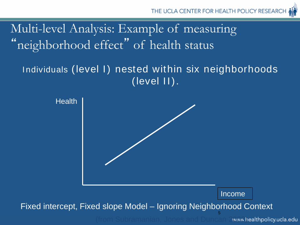
Multi-level Analysis: Example of measuring “neighborhood effect” of health status

Individuals (level I) nested within six neighborhoods (level II).

Health

Income

Fixed intercept, Fixed slope Model – Ignoring Neighborhood Context (from Subramanian, Jones and Duncan 2003)

6

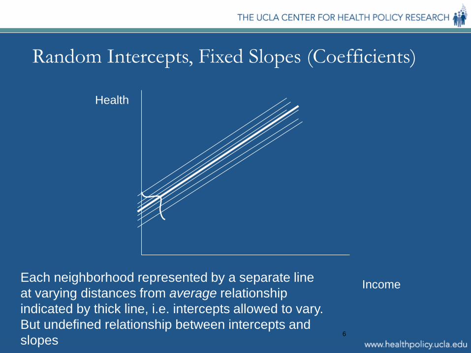
Random Intercepts, Fixed Slopes (Coefficients)

Health

Income Each neighborhood represented by a separate line at varying distances from average relationship indicated by thick line, i.e. intercepts allowed to vary. But undefined relationship between intercepts and slopes

7

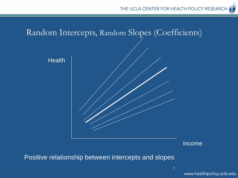
Random Intercepts, Random Slopes (Coefficients)

Health

Income

Positive relationship between intercepts and slopes

8

MLM: Conceptual Overview (1)

Example: 2-level case with a

continuous outcome. Individuals nested within

neighborhoods. J neighborhoods in total

and the jth neighborhood has nj people.

nj do not have to be equal across neighborhoods.

Level I (“within”) is individuals. Level II (“between”) is neighborhoods.

1 2 3 4 5 6 7 8 9

A B C

…..n

…..j

Level I patient

Level II hospital

9

MLM: Conceptual Overview

In practice, equations for all levels estimated simultaneously. More intuitive to think in terms of two separate sets of

regressions Makes it clear that one needs sufficient sample sizes at both

levels for the estimation to work. If the number of sites is small (typically less than ten), then it

is difficult to have the power at Level II to model many covariates.

For detailed discussion of power and sample size considerations see

Subramanian, Jones, Duncan’s chapter in Kawachi & Berman’s Neighborhoods and Health.

10

MLM: Level I Regression

Level I (“within”) is a series of J separate regressions, one for each level II unit (neighborhood).

The unit of observation for each of the J regressions is the person and the sample size for the jth regression is nj.

Yij = β0j + β1jXij + εij i = 1, …, nj

11

MLM: Level II Regression

Level II “Between” is a series of regressions, one for each random effect (either intercept or slope) in the model. The unit of observation for each regression is the neighborhood.

β0j = γ00 + γ01Wj + υ0j j = 1, …, J β1j = γ10 + γ11Wj + υ1j j = 1, …, J where Wj = level II covariate, e.g., neighborhood poverty β0j = intercept estimated using data for the jth level II

unit (neighborhood)

Yij = β0j + β1jX1ij + εij i = 1, …, nj Level I

12

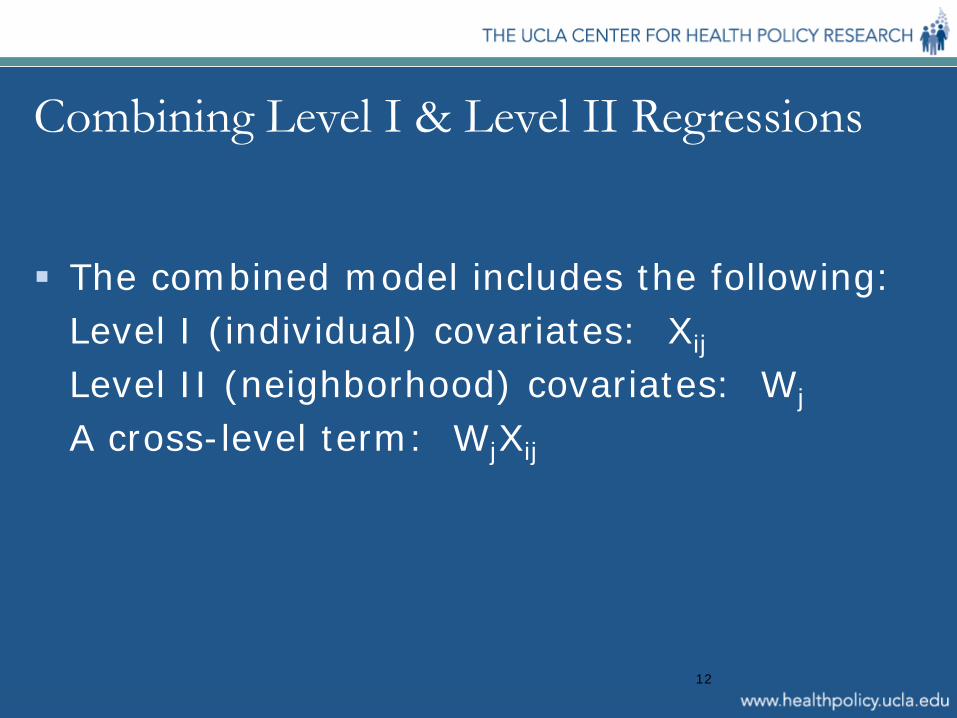
Combining Level I & Level II Regressions

The combined model includes the following: Level I (individual) covariates: Xij Level II (neighborhood) covariates: Wj

A cross-level term: WjXij

13

Combining Level I & Level II Regressions Single level models assumes one variance: σ2. This is not the case here, since people within the

same neighborhood are correlated in terms of υ0j + υ1j and the variances may be different.

υ0j + υ1jXij + εij is the MLM variance Note that this is an interactive model, because the

cross-level term allows neighborhood characteristics to modify the effect of the person’s characteristics living in her/his neighborhood.

14

Advantages of MLM

The question arises as to when multi-level models should be used instead of a single equation model like GEE.

15

Advantages of MLM over GEE

More efficient than alternative, non-parametric methods (e.g. GEE). Can model more than 2 levels. Can profile or rank by cluster

16

Disadvantages of MLM Multi-level models are less robust, more difficult to

estimate than other methods of dealing with clustering.

Depending on how the model is specified and the level at which covariates are measured, the sample size constraints can be binding.

Need to think about having sufficient sample size at all levels of the model.

Conceptual tradeoff between MLM and survey weights

17

MLMs vs. Single-level Models However, the greater complexity of multi-level

models is not always justified. A general rule of thumb is that if you are interested

in the actual identity of the level II unit (census tract, service planning area, etc.), e.g., for purposes of ranking, then you want to use MLM’s.

18

MLMs vs. Single-level Models

Suppose you don’t care about identifying particular units Not interested in identifying units as “better” or “worse” than

others Interested only about estimating the effects of the

characteristics of level II units e.g., neighborhood SES

In that case, simpler models (e.g., GEE) often suffice.

Various approaches to multilevel modeling outside of traditional hierarchical models

Estimate as single-level

Use survey weights—a type of GEE

Random effects models—a type of MLM

Study 1 - Background

Cordasco KM, et al. J Immigr Minor Health. 2011 Apr;13(2):260-7.

What is the relationship between distance to the nearest safety net clinic and access to healthcare in non-rural uninsured adults?

• People without insurance often access primary health care through the core healthcare safety net—a patchwork of providers predominantly composed of publicly-supported hospitals and safety net clinics (SNCs), such as community health centers

• The structure of the safety net varies widely across communities, most

commonly reflecting the community’s finances, politics, history and needs

Methodological Approach Using the 2005 California Health Interview Survey and a list of safety net

clinics, we calculated distance between uninsured interviewee residence and the exact address of the nearest clinic (ArcGIS)

Used multivariate regression to examine associations between this distance and interviewee’s probability of having a usual source of health care and having visited a physician in the prior 12 months.

Single level linear model

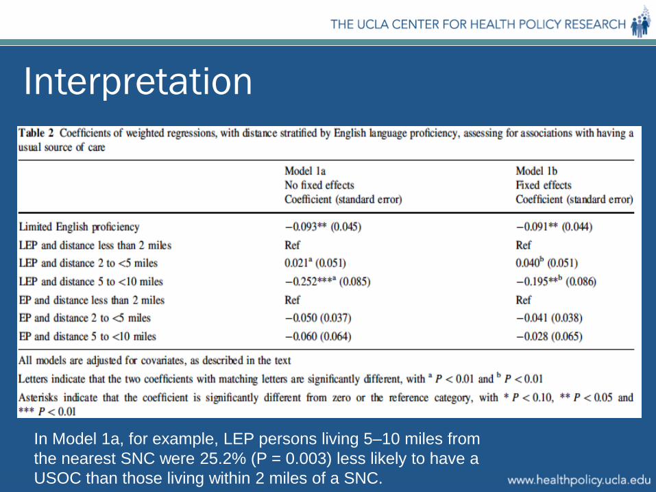
Interpretation

In Model 1a, for example, LEP persons living 5–10 miles from the nearest SNC were 25.2% (P = 0.003) less likely to have a USOC than those living within 2 miles of a SNC.

Study 2 – Background

What is the relationship between the Latino immigrant composition of neighborhoods in Chicago and various hypertension-related outcomes among Latinos?

Viruell-Fuentes EA, Ponce NA. J Immigr Minor Health. 2012 Dec;14(6):959-67.

• Latinos are less likely than non-Latino Whites to be screened and treated for hypertension, and to have their hypertension controlled

• At the individual level, lower levels of health insurance coverage and less access to care among Latinos are likely factors underlying these disparities

• In addition, socio-demographic and economic features of neighborhoods

and their attendant access (or lack thereof) to health-promoting resources may also contribute to health care disparities.

Methodological Approach Using 2001–2003 data Chicago Community Adult Health Study, stratified

into 343 neighborhood clusters (NCs) with meaningful physical and social boundaries The resulting neighborhood clusters included two contiguous census tracts that approximated

local neighborhoods Neighborhood variables used in the analyses represent continuous neighborhood-level measures

constructed from 20 variables from the 2000 Census via principal factor analysis

Used logistic regression to examine the associations between the neighborhood characteristics and (1) having hypertension, (2) utilizing hypertension-related health care, and (3) being treated for hypertension Used survey weights to account for selection rates, household size, neighborhood clustering

using complex survey feature in STATA

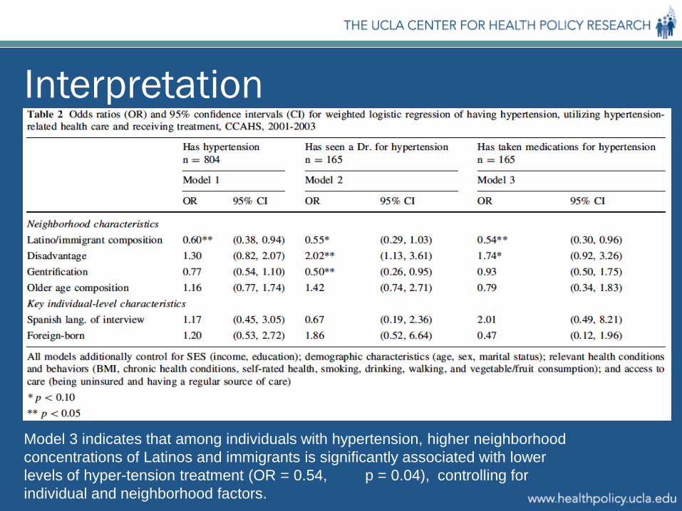
Interpretation

Model 3 indicates that among individuals with hypertension, higher neighborhood concentrations of Latinos and immigrants is significantly associated with lower levels of hyper-tension treatment (OR = 0.54, p = 0.04), controlling for individual and neighborhood factors.

Study 3 - Background

Do HMO market level factors differentially impact Asian American and Pacific Islanders’ (AAPIs’) adults with a family history of colorectal cancer (CRC) access to CRC screening compared with whites with a family history of CRC?

Ponce NA, et al. Med Care. 2005 Nov;43(11):1101-8.

• Few studies measure whether and to what extent health care market structure increases cancer screening among AAPI subjects, a group that has been typically underrepresented in disparities literature, despite population-based evidence of lower rates in breast, cervical, and CRC test use.

• We posit that area-level effects may explain some of the differences in AAPI–white cancer screening disparities, beyond individual-level risk factors, including type of health insurance and health care plan

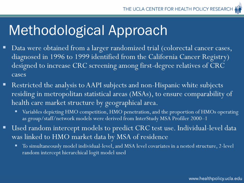
Methodological Approach Data were obtained from a larger randomized trial (colorectal cancer cases,

diagnosed in 1996 to 1999 identified from the California Cancer Registry) designed to increase CRC screening among first-degree relatives of CRC cases

Restricted the analysis to AAPI subjects and non-Hispanic white subjects residing in metropolitan statistical areas (MSAs), to ensure comparability of health care market structure by geographical area. Variables depicting HMO competition, HMO penetration, and the proportion of HMOs operating

as group/staff/network models were derived from InterStudy MSA Profiler 2000–1

Used random intercept models to predict CRC test use. Individual-level data was linked to HMO market data by MSA of residence To simultaneously model individual-level, and MSA level covariates in a nested structure, 2-level

random intercept hierarchical logit model used

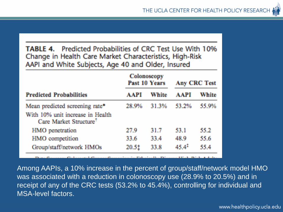
Raw output for multilevel logit difficult to interpret, and suggest using predicted probabilities—next slide

Among AAPIs, a 10% increase in the percent of group/staff/network model HMO was associated with a reduction in colonoscopy use (28.9% to 20.5%) and in receipt of any of the CRC tests (53.2% to 45.4%), controlling for individual and MSA-level factors.

Thank you!