+ All Categories
Home > Documents > CREATES Research Paper 2009-31 A No Arbitrage Fractional ... · Range-based volatility estimator,...

CREATES Research Paper 2009-31 A No Arbitrage Fractional ... · Range-based volatility estimator,...

Date post: 13-Mar-2020
Category:
Upload: others
View: 2 times
Download: 0 times
Share this document with a friend
36
School of Economics and Management Aarhus University Bartholins Allé 10, Building 1322, DK-8000 Aarhus C Denmark CREATES Research Paper 2009-31 A No Arbitrage Fractional Cointegration Analysis Of The Range Based Volatility Eduardo Rossi and Paolo Santucci de Magistris
Transcript

School of Economics and Management Aarhus University

Bartholins Allé 10, Building 1322, DK-8000 Aarhus C Denmark

CREATES Research Paper 2009-31

A No Arbitrage Fractional Cointegration Analysis Of The Range Based Volatility

Eduardo Rossi and Paolo Santucci de Magistris

A No Arbitrage Fractional Cointegration Analysis Of

The Range Based Volatility ∗

Eduardo Rossi† Paolo Santucci de Magistris‡

July 15, 2009

Abstract

The no arbitrage relation between futures and spot prices implies an analogous relation

between futures and spot volatilities as measured by daily range. Long memory fea-

tures of the range-based volatility estimators of the two series are analyzed, and their

joint dynamics are modeled via a fractional vector error correction model (FVECM), in

order to explicitly consider the no arbitrage constraints. We introduce a two-step esti-

mation procedure for the FVECM parameters and we show the properties by a Monte

Carlo simulation. The out-of-sample forecasting superiority of FVECM, with respect to

competing models, is documented. The results highlight the importance of giving fully

account of long-run equilibria in volatilities in order to obtain better forecasts.

Keywords. Range-based volatility estimator, Long memory, Fractional cointegration,

Fractional VECM, Stock Index Futures.

J.E.L. classification. C32, C13, G13.

∗We would like to thank Giuseppe Cavaliere, Katarzyna Łasak for very helpful and constructive comments

on an earlier version of this paper. We also thank the participants to the CREATES seminar.†Dipartimento di economia politica e metodi quantitativi, Via San Felice 5,University of Pavia, Italy. Cor-

responding author. Tel.: +39 0382/986207 Fax: +39 0382/304226. E-mail address: [email protected]. Financial

support from PRIN 2006 is gratefully acknowledged.‡Dipartimento di economia politica e metodi quantitativi, University of Pavia, Italy. Paolo Santucci de

Magistris thanks CREATES, funded by the Danish National Research Foundation, for hospitality.

1

Introduction

The relationship between spot and futures prices is a widely studied topic in the financial

literature. Since the introduction of future contracts during the 1970s, a great effort has

been made by academics and practitioners in understanding the pricing of future contracts.

Considering forward contracts, the no arbitrage assumption implies that, in a friction-

less market, the spot and the forward prices, under risk neutral probability, are related

by:

Ft|t−k = St−k · ek·rt|t−k (1)

where rt|t−k is the return of a risk free asset that expires in period t and ek·rt|t−k is referred

to as the cost of carry premium.

We investigate to what extent the no arbitrage condition in (1) induces a long run rela-

tionship between spot and futures volatilities, when, as in Parkinson (1980), Garman and

Klass (1980), Wiggins (1992) and Alizadeh et al. (2002), we adopt as a measure of daily

integrated volatility the daily range. We also show how the information implicit in the

future contracts could be exploited in forecasting the volatility of spot prices.

Daily range is equal to the difference between the highest and lowest log price of a given

day

Rt = maxτ

logPτ − minτ

logPτ (2)

where Pτ is the asset price at time t − 1 < τ ≤ t. As noted by Andersen and Bollerslev

(1998), the accuracy of the high-low estimator is near that provided by the realized volatil-

ity estimator based on 2 or 3 hours returns. Daily range-based volatility estimator is still 5

times more efficient than the traditional daily squared returns, see Christensen and Podol-

skij (2007).

Combining equation (1) and (2) and assuming that the risk free rate is constant with re-

spect to τ , we obtain a no arbitrage equilibrium relationship between the forward and spot

ranges,

RFt = RS

t . (3)

Under the hypothesis that spot log price evolves as a random walk in continuous time, with

the diffusion parameter ωτ such that ωτ = ωt ∀ τ ∈ (t− 1, t), an unbiased estimator of daily

2

integrated volatility, σ2t , is equal to

σ2t = 0.361 ·R2

t . (4)

where, as demonstrated in Parkinson (1980), Et−1[σ2t ] = ω2

t and MSEt−1[σ2t ] = 0.4073ω4

t ,

which is approximately one-fifth of the MSE of the daily squared return. We can then

recast equation (3) as

log σt,F = log σt,S . (5)

The equality in (5) is implied by the no-arbitrage pricing relationship in (1).

However, as pointed out in Andersen et al. (2001), Andersen et al. (2003), and Lieber-

man and Phillips (2008), volatilities can be assumed neither as an I(0) nor as an I(1) pro-

cess, but we should consider that they can be best approximated by a fractionally inte-

grated process, or I(d), where the parameter d can take any real value. in particular, when

we model the relation between log-ranges we have to allow for the possibility that they

can be fractionally cointegrated. In fact, the traditional cointegration concept only allows

for an integer order of integration in the equilibrium error process. This assumption ap-

pears to be too restrictive here. Fractional cointegration refers to a generalization of the

concept of cointegration, that is linear combinations of I(d) processes are I(d − b), with

0 < b ≤ d. This corresponds to the idea that there exists a common stochastic trend, that is

integrated of order b > 0, while the short period departures from the long run equilibrium

are integrated of order d − b ≥ 0. b stands for the fractional order of reduction obtained

by the linear combination of I(d) variables. Christensen and Nielsen (2006) applied the

concept of fractional cointegration in examining the relationship between implied and re-

alized volatility, estimating the cointegration vector in a regression setup. Cheung and Lai

(1993) applied the concept of fractional cointegration in studying the purchase power par-

ity hypothesis with a parametric model, and Duecker and Startz (1998) investigated the

relationship between bond rates estimating a bivariate long memory model, restricted in

order to allow for cointegration. Robinson (1994) showed inconsistency of OLS estimator

in the usual cointegration regression when the regressors are fractionally integrated, and

proposed an estimation approach based on frequency domain least squares. Christensen

and Nielsen (2006) derived the asymptotic distribution of the estimators in the stationary

case, i.e. d < 12 , while Robinson and Marinucci (2003) provided the limiting distribution

3

in the case d > 12 . Christensen and Nielsen (2006) studied the fractional cointegration re-

lationship between realized and implied volatilities, finding that their common fractional

order of integration is reduced by a linear combination of them. More recently, many au-

thors focused on the estimation of the cointegration rank. In particular, Robinson and

Yajima (2002) derived a formal semiparametric test for the cointegration rank based on

the spectral representation of the system. Nielsen and Shimotsu (2007), extended the

analysis of Robinson and Yajima (2002), proposing a fractional cointegration testing proce-

dure based on the exact Whittle estimator for both stationary and nonstationary processes.

Breitung and Hassler (2002) provided a test based on a multivariate trace test, similar to

that proposed by Johansen (1988), that is based on the solution of a generalized eigenvalue

problem. However, they consider only the cointegration relation between non-stationary

variables, such that d > 0.5.

In this paper, we jointly model the dynamics of future and spot volatility via the fractional

cointegration system outlined in Granger (1986), that is a generalization of the vector

ECM. The fractional VECM (FVECM hereafter), allows for a flexible characterization of

the cointegration relation, in the sense that the integration orders of the endogenous vari-

ables, d, and the cointegration residuals, d − b, are not restricted to assume values 1 and

0, respectively. On the other hand, the estimation procedure presents an additional diffi-

culty with respect to the standard VECM, since two additional parameters, d and b, need

to be estimated. Lasak (2008) suggests a profile likelihood procedure that allows to firstly

estimate b, while d is set to 1. In this paper, we provide an extension of the estimation

procedure outlined in Lasak (2008), carrying out a new inference method that maximizes

the profile likelihood in terms of both d and b, obtaining a joint estimate of them. A Monte

Carlo simulation assesses the ability of the profile maximum likelihood procedure to cor-

rectly estimate the true parameters of the model, showing that the estimated parameters

converge to the true values when the sample size increases. An out-of-sample forecasting

exercise is then carried out in order to verify the capacity of FVECM, which includes an er-

ror correction term based on a no arbitrage restriction, to lead to significant improvements

on models which do not account for the long run equilibrium. As expected, we find that

FVECM consistently outperforms the competing models in terms of accuracy of forecasts.

This evidence clearly confirms that imposing the no arbitrage condition produces superior

long-horizon forecasts.

4

The paper is organized as follows. Section 1 presents a brief description of the data and

the analysis of the long memory property of range-based volatility estimator, assessing the

equality of the integration orders between spot and future volatility and showing that the

two series have to be considered fractionally cointegrated. Given the evidence provided

in section 1, section 2 introduces the FVECM, as in Granger (1986) and Davidson et al.

(2006), in order to jointly model the dynamics of fractionally cointegrated series. Section

3 introduces the estimation method adopted, and section 4 reports the estimation results.

Section 5 provides evidence in favor of the FVECM in terms of forecasting ability and

section 6 concludes.

1 Data and Preliminary Analysis

The data used in this paper consist of the high and low daily spot and future prices on

the S&P500 index for the period 27th November 1998 to 5th September 2008 for a total

of 2450 trading days. The future prices are relative to the 3 months future contracts.

Given the long period of time under analysis, it seems natural to analyze the possible

presence of structural breaks in the series of log daily volatilities. In fact, as pointed out

by Granger and Hyung (2004), the long memory property of volatility could be induced

spuriously by the presence of structural breaks. For this reason, we search for structural

changes in the series under analysis, following the procedure outlined by Bai and Perron

(2003). In the following analysis we will refer to the residuals of the Bai-Perron procedure

as the demeaned series while the original series will be called raw. The temporal dynamics

of the series are very close each other, and the breakpoints are found to have the same

intensity in correspondence of the same observations.1. It is well known that volatility

series are clustered and present a slow (hyperbolic) decay of the autocorrelation functions,

see Andersen et al. (2001), that refer to this feature as induced by the presence of long

memory. Long memory is defined in terms of decay rates of long-lag autocorrelations, or in

the frequency domain in terms of rates of explosion of low frequency spectra. A long-lag

autocorrelation definition of long memory is

γ(τ) = cτ2d−1 τ → ∞ (6)

5

the correlations of long memory process decay with a hyperbolic rate. They are not summable.

An alternative, although not equivalent, definition of long range dependence can be ob-

tained in terms of the spectral density f(λ) of the process:

limλ→0+

f(λ)

cf |λ|−2d= 1 0 < cf <∞. (7)

The spectral density f(λ) has a pole and behaves like a constant cf times λ−2d at the ori-

gin. If |d| ∈ (0, 1/2) the process is stationary. In particular, if d ∈ (0, 1/2), it presents long

memory; instead, if d ∈ (−1/2, 0) the process is antipersitent with short memory. A popular

approach to the modeling of long memory is represented by the ARFIMA class introduced

by Granger and Joyeux (1980) and Hosking (1981).

Figure 1 displays the autocorrelation functions of the original volatility series with respect

to the residual series from the breakpoint searching analysis. The evidence from the ACF

is clearly supportive of the long memory property of the volatility series since the autocor-

relation functions decay very slowly. However, the reduction in the persistence obtained

by removing the breaks from the original series is evident. Even if the sensible reduction

in the persistence, the residual series still display a certain level of long memory. Given

the equilibrium relation stated in equation (5), we test for the possibility of fractional coin-

tegration considering both the raw series and the demeaned series. Robinson and Yajima

(2002) discuss a semi-parametric procedure for determining the cointegration rank, focus-

ing on stationary series. Nielsen and Shimotsu (2007) extend the analysis of Robinson and

Yajima (2002), in order to consider cointegration for both stationary and non-stationary

variables. In particular, they apply the exact local Whittle analysis in a multivariate setup,

see Shimotsu and Phillips (2005), and estimate the rank of spectral cointegration of the dth

differenced process by examining the rank of the spectral matrix, G, around the origin. As

pointed out by the authors, their approach does not require the estimation of any cointe-

gration vector, but it relies on the choice of bandwidths and threshold parameters.

Since the presence or absence of cointegration is not known when the fractional integration

order is estimated, they propose, as in Robinson and Yajima (2002), a test statistic for the

equality of integration orders that is informative in both circumstances, in the bivariate

case

T0 = m(Sd)′(S

1

4D−1(G⊙ G)D−1S′ + h(T )2

)−1

(Sd) (8)

6

where ⊙ denotes the Hadamard product, S = [1,−1]′, h(T ) = log(T )−k for k > 0 , D =

diag(G11, G22), while G = 1m

∑mj=1Re(Ij) and Ij is the coperiodogram at the frquency λj

(see Nielsen and Shimotsu (2007) for more details). The parameter d is the exact Local

Whittle estimator of d, introduced by Shimotsu and Phillips (2005). If the variables are not

cointegrated, that is the cointegration rank r is zero, T0 → χ21, while if r ≥ 1, T0 → 0. A

significantly large value of T0, with respect to χ21, can be taken as an evidence against the

equality of the integration orders.

Moreover, the estimation of the cointegration rank r is obtained by calculating the eigen-

values of the estimated matrix G. The estimator G uses a new bandwidth parameter n. Let

δi the ith eigenvalue of G, it is possible to apply a model selection procedure to determine

r. In particular,

r = arg minu=0,1

L(u) (9)

where

L(u) = v(T )(2 − u) −2−u∑

i=1

δi (10)

for some v(T ) > 0 such that

v(T ) +1

n1/2v(T )→ 0. (11)

Tables 1 and 2 show the results of the Nielsen and Shimotsu (2007) fractional cointegra-

tion analysis, with two different choices for the bandwidths, m, used in the estimation of

d’s in the exact local Whittle estimation, and n used in the estimation of G and L(u). The

estimates of the long memory parameter, d, are close to 1/2. Otherwise, when we consider

the residuals of the Bai and Perron (2003) procedure for the breaks (demeaned series), the

estimated d falls into the stationarity region for all bandwidths. The T0 statistic takes val-

ues close to 0 for both the raw data and demeaned series. The analysis of the cointegration

rank, in Panel B, confirms the presence of cointegration, in fact r = 1 in all cases. Since the

95% critical value of a χ21 is 3.841, we cannot reject the null of equality of the integration

orders in all cases. Interestingly, the series are fractionally cointegrated even if the pres-

ence of structural breaks is removed.

The result of the test of Nielsen and Shimotsu (2007) confirms that volatility of spot and

future prices have the same fractional integration order and are cointegrated.

Moreover, given the equality of the integration orders, we estimate the cointegrating vector

7

in a regression setup, as suggested by Engle and Granger (1987). Given the equilibrium

relation stated in equation (5), it seems to be natural to test empirically the difference

log σt,F − log σt,S = zt ∼ I(d− b) (12)

where b > 0 and zt is a stationary fractionally integrated variable with fractional order less

than d, i.e. dz = d− b < d. In this context, we call full cointegration the case in which b = d,

that is the case in which the order of integration of the residual is zero. The typical case

considered in empirical works is d = b = 1, that is Xt are I(1) and zt is I(0). Cointegration

requires that zt is mean reverting, that is a long run restriction on the dynamics of Xt.

A simple way to test this hypothesis is examining the degree of persistence of the residuals

of the following regression

log σt,F = β log σt,S + zt (13)

under the assumption that spot and future volatility have the same d. The parameter β is

estimated with the Frequency Domain Least Squares (FDLS), as suggested by Robinson

and Marinucci (2003). Since the series of demeaned series are stationary and present

long memory (the estimated d is between 0 and 0.5), we follow the approach suggested

by Christensen and Nielsen (2006). The parameter β is estimated with the Narrow Band

Frequency Domain Least Squares (NB-FDLS, hence after). 2 As noted by Robinson (1994)

and Robinson and Marinucci (2003), when xt is stationary, the βm is consistent for β due

to dominance of the spectrum of log σt,S over that of zt near zero frequency. Christensen

and Nielsen (2006) have derived the asymptotic distribution of βm when 0 < d < 12 and

0 < b < d. In particular, in the simple case of two variables, this is equal to

√mλdz−d

m (βm − β) → N

(0,

ge(1 − 2dx)2

2gx(1 − 2dx − 2dz)

)(14)

where ge and gx correspond to var(∆bzt) and var(∆dxt). The results of the procedure of

Christensen and Nielsen (2006) for different bandwidth, m, are presented in table 3. When

the demeaned series are taken into account, the estimates of β and d from table 3 strongly

supports the idea of fractional cointegration among the two series. In fact, the fractional

order of the residuals is close to zero, so that b ≈ d, and we get full cointegration. Moreover,

the estimated cointegration parameter, βm, is very close to 1, in particular when the NB-

8

FDLS are used instead of OLS.

On the other hand, when the cointegration regression is implemented on the raw data, we

are not able to compute the standard error of βm, since d + dz > 0.5. 3 Nevertheless, the

point estimate of βm is in all cases very close to the theoretical value 1, but the fractional

reduction of the integration order in this case is not complete, since dz ≈ 0.2. This result

can be explained by the presence of structural breaks, that are a source of non stationarity.

For this reason, the following analysis will be conducted on the demeaned series.

2 The Model

Given the analysis in the previous chapter, we propose to jointly model the dynamics of the

spot and future volatilities through a fractionally integrated vector error correction model

that accounts for their equilibrium relation. Differently from Davidson (2002) and Duecker

and Startz (1998), our series are stationary. We consider the Granger (1986) representa-

tion of fractionally cointegrated systems, that is the Fractionally Integrated Vector ECM

(FVECM) 4, given by

∆dXt = (1 − ∆b)(∆d−bαβ′Xt) +k−1∑

j=1

Γj∆dXt−j + ǫt t = 1, . . . , T (15)

where Xt = (log σt,F , log σt,S), and Γj are the short run matrices of parameters. ǫt is a in-

dependent identically distributed vector with mean 0 and covariance matrix Ω. α and β

are the error correction and cointegration matrices. Our setup slightly differs from the bi-

variate model proposed by Duecker and Startz (1998). Their model is a bivariate ARFIMA

process, with the additional restriction that the fractional difference of a linear combina-

tion of the two series is d− b ≥ 0; the cointegrating parameter β is treated as an additional

unknown parameter in constructing the Gaussian likelihood function (see Sowell (1989)

and Sowell (1992)). An alternative representation of fractionally cointegrated systems is

presented in Johansen (2008).

In the FVECM model, the element αij of the parameters matrix α measures the single

period response of variable i to the shock on the equilibrium relation j. In our case, j = 1

with α = (α1, α2)′, thus α1 should be negative in order to move toward the unique long

run relationship implied by the no arbitrage assumption. The vector coefficient α has a

9

clear interpretation as a short term adjustment coefficient and represents the proportion

by which the long run disequilibrium in the spot (futures) volatility is being corrected in

each period.

Omitting the vector autoregressive terms, our model is defined as

(1 − L)d log σt,F = α1((1 − L)(d−b) − (1 − L)d)(log σt,F − β log σt,S)) + ǫ1t

(1 − L)d log σt,S = α2((1 − L)(d−b) − (1 − L)d)(log σt,F − β log σt,S)) + ǫ2t

where the ǫt = (ǫ1t, ǫ2t) are assumed to be Gaussian with mean zero and variance Ω.

3 Estimation

As pointed out by Lasak (2008), the estimation procedure of the fractional vector error

correction model (15) presents an additional source of uncertainty with respect to the stan-

dard VECM (where d and b are restricted to be equal to 1), since the additional unknown

parameters d and b need to be estimated. A solution to this problem is provided by Lasak

(2008), that suggests to impose d = 1 and concentrate the likelihood function with respect

to b. In particular, the model (15) is estimated via a maximum likelihood technique analo-

gous to that developed by Johansen (1991) for the standard VECM, where the initial step

consists of maximizing the profile likelihood with respect to b. In our case, we do not re-

strict the parameter d to be equal to 1, but we propose to jointly estimate the parameters

d and b, by maximizing the profile likelihood with respect to both parameters at the initial

stage.

The estimation procedure begins defining Z0,t = ∆dXt and Z1,t = (∆d−b − ∆d)Xt while

Zk,t = (∆dXt−1, ...,∆dXt−k+1), so that the system (15) can be written as

Z0,t = αβ′Z1,t + ΓZk,t + ǫt, (16)

where Γ = (Γ1, ...,Γk−1). We define the matrix of cross product matrix as

Mij = T−1T∑

t=1

Zi,tZ′j,t i, j = 0, 1, k, (17)

10

so that the residual of the regression of Z0,t and Z1,t on Zk,t can be defined as

Ri,t = Zi,t −MikM−1kk Zk,t i = 0, 1. (18)

The residual sum of squares results to be:

Sij = Mij −MikM−1kk Mkj , (19)

where Sij depends on d and b, except when i = j = 0. For fixed d, b, α and β, Γ is estimated

as

Γ(d, b, α, β) = (M0k − αβ′M1k)M−1kk , (20)

For fixed d, b and β, α and Ω are estimated as

α(d, b, β) = S01β(β′S11β)−1, (21)

and

Ω(d, b, β) = S00 − α(β′S11β)α′. (22)

Plugging this estimates into the likelihood we get

L(d, b, α, β, Ω) = |S00 − S01β(β′S11β)−1β′S10|, (23)

that is maximized by the eigenvector corresponding to the r maximum eigenvalues that

solve the problem

|λS11 − S01S−100 S01| = 0 (24)

The vector β is estimated as the r-dimensional space spanned by the eigenvectors, vj for

j = 1, ..., r, corresponding to the r largest eigenvalues of S−111 S01S

−100 S01.

Given this choice of β, the likelihood function is maximized only with respect to d and b,

that is

(d, b) = argd,b maxL(d, b), (25)

where

LT (d, b) =

[|S00|

r∏

i=1

(1 − λi)

]−T

2

(26)

11

Once d and b are estimated, as the values that maximize the function L(b, d), all the other

parameter of model (15) are obtained as functions of d and b.

Note that β, α, Γ and Ω are all consistent estimator given that d and b are consistent

estimators of d and b, since when d and b are known to be estimated consistently, β, α, Γ and

Ω are also consistent estimates, given the Continuous Mapping Theorem and the results

in Johansen (1995). On the other hand, we conjecture that d and b exist and are consistent

estimates of d and b if the objective function in equation (26) is uniquely maximized at the

true point (d, b), that is LT (d, b) being concave. In appendix, we show, in Monte Carlo setup,

the consistency of all the estimators.

4 Results

System (15) for spot and future range-based volatility has been estimated using the pro-

cedure described in section 3. Since the number of lags included plays an important role

in this context, we first implement two information-based criteria for the model selection.

The Schwarz and Hannan-Quinn information criterion functions are minimized for p = 1

and p = 2 for respectively. The following analysis is based on p = 1.

The estimation results are reported in table 4.5 Table 4 also reports the bootstrapped

confidence interval of the parameters. The bootstrapped sample has been generated with

1000 replications of wild bootstrap, that is robust to heteroskedastic effects. Most of the

confidence intervals of the parameters does not contain the value 0, meaning that they

are statistically different from zero. β is very close to the NB-FDLS estimates obtained in

the previous section, and the theoretical value β = 1 is contained in the 90% confidence

interval. Moreover, the estimates of d and b are close to the values obtained in the semi-

parametric analysis in section 1. From a visual inspection of figure 2, it clearly appears

that the residual component of the cointegration relation does not have any long memory

feature, as confirmed by the semiparametric estimate of the parameter d, that is close to 0.

The vector α highlights the speed of adjustment to the long run equilibrium; the volatility

of the spot price returns faster to the equilibrium. Moreover, the bootstrapped 95th quan-

tile of α1 is positive, so that α1 cannot be considered statistically different from zero, and

there are no changes in the future volatility due to shocks in the cointegration relation. All

the corrections to the equilibrium are made by changes in the spot volatility. This means

12

that future volatility has to be considered weakly exogenous with respect to spot volatility

in this context, that is future volatility leads spot volatility to the equilibrium, implicitly

confirming the Cox (1976)’s hypothesis on the efficiency of the future market in processing

the new information.

5 Forecast

If the forecasting performances, at large horizons, depend on the model specification, then

allowing for a mechanism restoring the long-run equilibrium between future and spot

volatility, as in the fractional VECM could improve the forecasts. We evaluate the ac-

curacy of our model in forecasting volatility and we compare the out-of-sample forecasts of

FVECM with those provided by alternative model specifications. In particular, we consider

• Vector Autoregression model with 4 lags, V AR(4);

• Univariate HAR model, UHAR, proposed by Corsi (2009), where the observed log

volatility is regressed on its own daily, weekly and monthly past values

log σt = ω + β1 log σt−1 + β2Wt−1 + β3Mt−1 + ut

where Wt−1 = 15

∑5i=1 log σt−i and Mt−1 = 1

22

∑22i=1 log σt−i;

• Bivariate HAR, BHAR , where we include past values of the future (spot) log volatil-

ity in the equation of the spot (future) volatility:

log σFt = ω1 + β11 log σF

t−1 + β12WFt−1 + β13M

Ft−1 + β14 log σS

t−1 + β15WSt−1 +

+β16MSt−1 + ut,1

log σSt = ω2 + β21 log σF

t−1 + β22WFt−1 + β23M

Ft−1 + β24 log σS

t−1 + β25WSt−1 +

+β26MSt−1 + ut,2

The system’s parameters are estimated by least squares.

• ARFIMA(0,d,0) model, ARFIMA, that accounts for the long memory feature of the

data;

(1 − L)d log σt = ut (27)

13

where ut ∼ iiN(0, v2);

• FIVAR(p,d) model, FIV AR,:

Φ(L)(1 − L)d log σt = ut (28)

where Φ(L) is an autoregressive matrix polynomial so that the FIVAR could be con-

sidered a VAR calculated on the fractionally differenced series. 6

The forecasts are based on parameter estimates from rolling samples with fixed sample

size of 1350 days. For every date t ≥ 1350 in the sample, we estimate the parameters of

each specification over the 1350 observations up to and including date t. Then, we consider

the forecasts of the log volatilities of both assets over the period t + 1, ..., t + s, where s is

equal to 1, 5, and 22, respectively for daily, weekly and monthly horizon forecasts, so that

we have both short-term and long-term forecasts. We avoid the presence of overlapping

observations, meaning that the forecast sample is constituted by 50 monthly, 200 weekly

and 1100 daily forecasts (this approach has been followed for instance by Brandt and Jones

(2006)). The forecasts refer to the integrated log volatilities over the period (t + 1, t + s),

these are approximated by the daily log volatility, and by the averages over a week and a

month of the log volatilities as measured by the the log-adjusted range, that is

V t+1,t+s =1

s

s∑

τ=1

log σt+τ . (29)

The MSE, the RMSE, and the MAE statistics in Table 5 clearly depict a situation where the

FVECM outperforms the alternative models. We also evaluate the unbiasedness of the esti-

mates regressing the actual integrated log volatilities on a constant and the corresponding

out-of-sample forecast, the so-called Mincer and Zarnowitz (1969) regression:

V t+1,t+s = α+ βV jt+1,t+s + ut+1,t+s, (30)

where V jt+1,t+s is the average of model j forecasts over the period (t + 1, t + s). In Table 6

the coefficient estimates (Panel (a) and (b)) and the regression adjusted R2 (Panel (c)) are

reported. We also compute test statistic for the restriction that α = 0 and β = 1. Table 6

reports the results of the tests based on the regression in (30). It clearly emerges that the

FVECM, differently from alternative specifications, provides unbiased forecasts of the out-

14

of-sample log-volatility for all the different choices of s. This result turns out to be more

evident when considering longer forecast horizon, confirming that allowing for fractional

cointegration improves the forecasts. Table 6 reports also the adjusted R2 that is, in all

cases, higher than that obtained with other specifications, demonstrating superiority of

the FVECM in forecasting volatility.

We also test for the forecasting superiority of FVECM in the Diebold and Mariano (1995)

framework, focusing here on the mean squared error (MSE) of the forecasts, where the

error of model i at date t is defined as the difference, ǫi,t, between the sample average of

the log volatility in the period (t+1, t+s) and the corresponding forecast provided by model

i. Specifically, we are interested in measuring the relative forecasting performance of the

different model specifications, testing the superiority of model i over model j with a t-test

of the µij coefficient in

ǫ2i,t − ǫ2j,t = µij + ηt (31)

where a positive estimate of µij indicates support for model i. In our case, we evaluate all

the pairwise tests with respect to the FVECM model for all the choices of s. Table 6 reports

the t-statistics for the estimates of µij . It is clear that the forecasts based on the FVECM

specification provides in many cases an improvement with respect to the alternatives, since

the value of the t-test is always positive and, in many cases, significant. Moreover, it is in-

teresting to note the superiority of forecasts of the spot volatility at weekly and monthly

frequency, that is probably due to the convergence of spot volatility to the long run equi-

librium that is implicit in the FVECM. These results suggest that, properly accounting for

the long-run relation between volatilities, implicit in the no-arbitrage pricing, provides a

significant forecast improvement, since future volatility, given the speculative nature of

future contracts, leads spot volatility.

6 Conclusions

This paper focused on a no arbitrage cointegration relationship between two range based

volatility measures. Given the long memory property of the volatility series, the analy-

sis is carried out in terms of fractional cointegration so that the dynamic behavior of the

two series has been modeled by a fractional VECM model, as defined by Granger (1986).

The cointegrated system is estimated, implementing a new procedure, based on the profile

15

likelihood, that allows to jointly estimate d and b. This technique extends the estimation

method proposed in Lasak (2008). We confirm the presence of a common stochastic trend

with long memory that captures the total persistence of the system, so that the error cor-

rection term is integrated of order 0. Moreover the parameter β is close to the theoretical

value 1, while spot volatility converges faster toward the long run equilibrium than the

volatility of the future price. This evidence suggests that future volatility is the driving

factor in the volatility process, since futures contracts are more efficient in processing the

new information. Allowing the long range dependence, between spot and future volatility,

improves significantly the out-of-sample forecasts, given the equilibrium mechanism that

is incorporated in the model for fractional cointegration.

A Monte Carlo Simulation

The following Monte Carlo simulation is intended to asses the ability of the ML procedure,

outlined in section 3, to correctly estimate the true parameters of the model. In other

words, we wish to evaluate the consistency of our estimation procedure assuming that the

cointegration rank is known. We generate two fractionally cointegrated processes, from

the representation in Granger (1986), as

Yt = α1(∆−b − 1)(Yt−1 − βXt−1) + (1 − L)−dǫ1t

Xt = α2(∆−b − 1)(Yt−1 − βXt−1) + (1 − L)−dǫ2t (32)

We chose d = 0.4, β = 1 and α = (−0.5, 0.5). The parameter b assumes values 0.4 and 0.3.

The infinite moving-average representation of the long memory process, ut, is given by

ui,t = (1 − L)−dǫi,t =∞∑

i=0

ψiηi,t−i (33)

where ψi = id−1/(d− 1) as i→ ∞, see Hosking (1981).

From a practical point of view, we consider a truncated version of ((33)), that is

u+i,t = (1 − L)−dǫi,t =

t−1∑

i=0

ψiǫi,t−i (34)

16

where the presample values are assumed to be equal to zero.

We generate 1000 time series with T = 500, 1000, 2000 observations each. ǫ1t and ǫ2t are

randomly generated from bivariate normal distribution with mean 0 and variance 1, with

correlation equal to 0.9.7 All the parameters are then estimated following the method

presented in section 3.8 The precision in the estimation of the parameters increases dra-

matically with the sample size. This is due to the long memory feature of the series under

exam. Moreover, the RMSE highlights the idea, already noted by Lasak (2008), that the

parameter dispersion increases with the difference between d and b. We obtain particu-

larly good estimates of β, also for moderate sample size. On the other hand, the estimates

of the vector α appear more volatile; this is due to the fact that α is function of d, b and β,

and it is sensible to the estimation uncertainty present in the previous steps. As shown in

graph 4, the estimates of α are positively skewed. This is due to the presence of outliers in

correspondence of values of b that are negative. Note that the skewness tends to zero when

b = d and T → ∞; that is when b is more precisely estimated and does not take negative

values. Since volatility of financial series often present GARCH effects, see for example

Corsi et al. (2005), we check for the robustness of our estimation procedure running again

the previous analysis, adding a multivariate GARCH component to the errors of equation

((32)). In particular, we define the conditional volatility of ǫt = (ǫ1t, ǫ2t)′ as the Constant

Conditional Correlation model, presented by Bollerslev (1990). The constant correlation

parameter, ρ, is set equal to 0.95, while the conditional GARCH(1,1) variances are

σ2i,t| = ωi + δiσ

2i,t−1|t−2 + γiǫ

2i,t−1 i = 1, 2 (35)

so that ǫt is distributed as a N(0,Σij,t), where Σij = ρσi,tσj,t for i 6= j and Σij,t = σ2i,t for

i = j. We select γi = 0.1, ωi = 0.05 and δi = 0.8 for i = 1, 2. The results from the Monte Carlo

exercise in presence of GARCH effects are also presented in table 9. The results seems to

confirm the robustness of our estimation procedure with respect to GARCH effects.

17

References

Alizadeh, S., Brandt, M. W., and Diebold, F. X. (2002). Range-based estimation of stochastic

volatility models. The Journal of Finance, Vol. 57, No. 3:pp. 1047–1091.

Andersen, T. and Bollerslev, T. (1998). Answering the skeptics: Yes, standard volatility

models do provide accurate forecasts. International Economic Review,, 39:885–905.

Andersen, T. G., Bollerslev, T., Diebold, F. X., and Ebens, H. (2001). The distribution of

stock return volatility. Journal of Financial Economics, 61:43–76.

Andersen, T. G., Bollerslev, T., Diebold, F. X., and Labys, P. (2003). Modeling and forecasting

realized volatility. Econometrica, 71:579–625.

Bai, J. and Perron, P. (2003). Computation and analysis of multiple structural change

models. Journal of Applied Econometrics, 18(1):1–22.

Bollerslev, T. (1990). Modelling the coherence in short-run nominal exchange rates: a

multivariate generalized arch approach. Review of Economics and Statistics, 72:498505.

Brandt, M. W. and Jones, C. S. (2006). Volatility forecasting with range-based egarch mod-

els. Journal of Business & Economic Statistics, Vol. 24, No. 4:470–486.

Breitung, J. and Hassler, U. (2002). Inference on the cointegration rank in fractionally

integrated processes. Journal of Econometrics, 110(2):167–185.

Cheung, Y. and Lai, K. (1993). A fractional cointegration analysis of purchasing power

parity. Journal of Business and Economic Statistics, 11:103122.

Christensen, B. J. and Nielsen, M. . (2006). Semiparametric analysis of stationary frac-

tional cointegration and the implied-realized volatility relation. Journal of Economet-

rics.

Christensen, K. and Podolskij, M. (2007). Realized range based estimation of integrated

variance. Journal of Econometrics, 141:323–349.

Corsi, F. (2009). A simple approximate long-memory model of realized volatility. Journal

of Financial Econometrics, 7:174–196.

18

Corsi, F., Kretschmer, U., Mittnik, S., and Pigorsch, C. (2005). The volatility of realized

volatility. CFS Working Paper Series 2005/33, Center for Financial Studies. available at

http://ideas.repec.org/p/cfs/cfswop/wp200533.html.

Cox, C. C. (1976). Futures trading and market information. The Journal of Political Econ-

omy, 84:1215–1237.

Davidson, J. (2002). A model of fractional cointegration, and tests for cointegration using

the bootstrap. Journal of Econometrics, 110(2):187–212.

Davidson, J., Peel, D., and Byers, J. (2006). Support for governments and leaders: Frac-

tional cointegration analysis of poll evidence from the uk, 1960-2004. Studies in Nonlin-

ear Dynamics & Econometrics, 10(1):1345–1345.

Diebold, F. X. and Mariano, R. S. (1995). Comparing predictive accuracy. Journal of Busi-

ness & Economic Statistics, 13(3):253–63.

Duecker, M. and Startz, R. (1998). Maximum likelihood estimation of fractional cointe-

gration with an application to us and canadian bond rates. Review of Economics and

Statistics, 80:420426.

Engle, R. F. and Granger, C. W. J. (1987). Co-integration and error correction: Representa-

tion, estimation, and testing. Econometrica,, 55, issue 2:251–76.

Garman, M. B. and Klass, M. J. (1980). On the estimation of security price volatilities from

historical data. Source: The Journal of Business,, Vol. 53, No. 1:67–78.

Granger, C. W. and Hyung, N. (2004). Occasional structural breaks and long memory with

application to the s&p 500 absolute stock returns. Journal of Empirical Finance, 11:399–

421.

Granger, C. W. J. (1986). Developments in the study of cointegrated economic variables.

Oxford Bulletin of Economics and Statistics, 48(3):213–28.

Granger, C. W. J. and Joyeux, R. (1980). An introduction to long-memory time series models

and fractional differencing. Journal of Time Series Analysis, 4:221–238.

Hosking, J. (1981). Fractional differencing. Biometrika, 68:165–76.

19

Johansen, S. (1988). Statistical analysis of cointegration vectors. Journal of Economic

Dynamics and Control, 12:231–254.

Johansen, S. (1991). Estimation and hypothesis testing of cointegration vectors in gaussian

vector autoregressive models. Econometrica, 59(6):1551–80.

Johansen, S. (1995). Likelihood-Based Inference in Cointegrated Vector Autoregressive Mod-

els. Oxford University Press, Oxford.

Johansen, S. (2008). A representation theory for a class of vector autoregressive models for

fractional processes. Econometric Theory, Vol 24 ,3.

Lasak, K. (2008). Maximum likelihood estimation of fractionally cointegrated systems.

Technical report, CREATES Research Paper 2008-53.

Lieberman, O. and Phillips, P. C. B. (2008). Refined inference on long-memory in realized

volatility. Econometric Reviews, 27(1):254–267.

Mincer, J. A. and Zarnowitz, V. (1969). The evaluation of economic forecasts. Nber working

papers, National Bureau of Economic Research, Inc.

Nielsen, M. . and Shimotsu, K. (2007). Determining the cointegration rank in nonsta-

tionary fractional system by the exact local whittle approach. Journal of Econometrics,

141:574–596.

Parkinson, M. (1980). The extreme value method for estimating the variance of the rate of

return. The Journal of Business, 53:61–65.

Robinson, P. M. (1994). Semiparametric analysis of long-memory time series. The Annals

of Statistics, 22(1):515–539.

Robinson, P. M. and Marinucci, D. (2003). Semiparametric frequency domain analysis of

fractional cointegration. In Robinson, P. M., editor, Time Series with Long Memory, pages

334–373. Oxford University Press.

Robinson, P. M. and Yajima, Y. (2002). Determination of cointegrating rank in fractional

systems. Journal of Econometrics, 106:217–241.

Santucci de Magistris, P. and Christensen, B. (2009). Fractional cointegration and level

shifts in the realized and implied volatility relation. Technical report, Aarhus University.

20

Shimotsu, K. and Phillips, P. (2005). Exact local whittle estimation of fractional integra-

tion. Annals of Statistics, 33:18901933.

Sowell, F. (1989). Maximum likelihood estimation of fractionally integrated time series

models. Technical report, unpublished manuscript Carnegie-Mellon University.

Sowell, F. (1992). Maximum likelihood estimation of stationary univariate fractionally

integrated time series models. Journal of Econometrics, 53(1-3):165–188.

Wiggins, J. B. (1992). Estimating the volatility of s&p 500 futures prices using the extreme-

value method. Journal of Futures Markets, v12(3):265–274.

Notes

1In a recent paper, Santucci de Magistris and Christensen (2009) note that the presence of a common level

shifts process among two or more I(0) series induces spurious fractional cointegration. Our purpose, in this

section, is to show that fractional cointegration between spot and future volatility is not induced spuriously by

the presence of common shifts but it is due to their common stochastic trend. However, we are aware of the

fact that a more efficient inference technique could be implemented, providing a synthesis between the concept

of fractional cointegation and the idea of structural breaks, in order to carry out a new testing procedure to

distinguish between the two sources of common persistence. This is left for future research.

2Christensen and Nielsen (2006) used m = 3, 6, 9, 15.

3This correspond to the case I in Robinson and Marinucci (2003), for which a asymptotic distribution for β

is not explicitly defined.

4Johansen (2008) proposes an alternative parametrization that allows for a Granger representation of co-

fractional systems, where the short run terms are written in terms of the new lag operator Lb = 1 − (1 − L)b.

On the other hand, the ECM term is the same in both models and the Granger (1986) representation has been

already considered by Lasak (2008) with inference purposes.

5The model also includes Γ10. In this way, the model accounts for a significant spike in the autocorrelations

at the 10−th lag.

6Even if a correct, but very slow, procedure has been implemented to estimate the FIVAR, see Sowell (1992),

we deal with a faster two step estimation method that consists of estimating first the fractional parameter d

and then calculating the VAR on the fractionally filtered series.

7This choice is motivated by the wish to resemble the statistical properties of the observed data.

8Note that all the parameters are left free to vary over all ℜ.

21

Raw Data

m = T 0.7 = 235 m = T 0.6 = 108 m = T 0.5 = 49

log σt,F 0.4797 0.5715 0.5188(0.0639) (0.0943) (0.1400)

log σt,S 0.4909 0.5636 0.5375(0.0639) (0.0943) (0.1400)

T0 0.1653 0.0452 0.1247

Demeaned series

m = T 0.7 = 235 m = T 0.6 = 108 m = T 0.5 = 49

log σt,F 0.4147 0.4851 0.2715(0.0639) (0.0943) (0.1400)

log σt,S 0.4313 0.4753 0.3101(0.0639) (0.0943) (0.1400)

T0 0.3600 0.0690 0.5300

Table 1: Fractional integration estimation with exact local Whittle estimator (standard error in parenthesis). The T0 test statistic is

calculated with h(T ) = log(T ).

22

Raw Data Demeaned series

L(u) v(T ) = n−0.45 v(T ) = n−0.35 v(T ) = n−0.25 L(u) v(T ) = n−0.45 v(T ) = n−0.35 v(T ) = n−0.25

m = 235,n = 109L(0) −1.7956 −1.6607 −1.4368 L(0) −1.7956 −1.6607 −1.4368L(1) −1.8457 −1.7762 −1.6682 L(1) −1.8452 −1.7778 −1.6688r 1 1 1 r 1 1 1

m = 108,n = 50L(0) −1.7099 −1.5545 −1.3158 L(0) −1.7099 −1.45545 −1.3158L(1) −1.8326 −1.7549 −1.6355 L(1) −1.8321 −1.7523 −1.6350r 1 1 1 r 1 1 1

m = 49,n = 22L(0) −1.5883 −1.4118 −1.1655 L(0) −1.5853 −1.4118 −1.1655L(1) −1.7836 −1.6968 −1.5737 L(1) −1.7826 −1.6959 −1.5727r 1 1 1 r 1 1 1

Table 2: Fractional cointegration estimation. The table reports the value of the function L(u) for different choices of m and n.

23

Demeaned series

Bandwidth βm s.e.(βm) dz s.e.(dz)

m = T − 1 0.8938 −− 0.1147 (0.0483)m = 20 0.9845 0.0310 0.0118 (0.0483)m = 15 0.9885 0.0332 0.0103 (0.0483)m = 9 0.9754 0.0420 0.0165 (0.0483)m = 6 1.0147 0.0517 0.0088 (0.0483)

Raw Series

Bandwidth βm s.e.(βm) dz s.e.(dz)

m = T − 1 0.9475 −− 0.2895 (0.0483)m = 20 1.0373 −− 0.2034 (0.0483)m = 15 1.0415 −− 0.2024 (0.0483)m = 9 1.0435 −− 0.2021 (0.0483)m = 6 1.0494 −− 0.2018 (0.0483)

Table 3: Fractional Cointegration Analysis: the estimation of β is performed with m = T −1, 20, 15, 9, 6, while dz is obtained with the Whittle

estimator with the bandwidth equal to T 0.6

24

d 0.3717 α1 −0.1979(0.3357, 0.4080) (−0.4757 , 0.07039)

b 0.3717 α2 0.7436(0.2326 , 0.5253) (0.4753 , 1.0229)

β −1.0081(−1.0387,−0.9795)

γ111 −0.1631 γ10

11 0.0753(−0.2602, −0.0690) (0.0026, 0.1426)

γ112 −0.0599 γ10

12 −0.0026(−0.1557, 0.0346) (−0.0703, 0.0656)

γ121 −0.0820 γ10

21 0.0932(−0.1815, 0.0153) (0.0193, 0.1681)

γ122 −0.1689 γ10

22 −0.0238(−0.2672, −0.0677) (−0.0967, 0.0478)

JBF 0.2343 JBS 0.7993LMF 0.1690 LMS 0.5771

Table 4: Estimation Results. Table reports the estimated parameter values. In parenthesis the 5th and 95th bootstrapped quantiles. JBF

and JBS are the p-values of Jarque-Bera test of normality for spot and future volatility, while LMF and LMS are p-values of Godfrey test of

heteroschedasticity for spot and future volatility.

25

(a) Futures

MSE RMSE MAE

s = 1 s = 5 s = 22 s = 1 s = 5 s = 22 s = 1 s = 5 s = 22V AR(4) 0.178 0.067 0.078 0.423 0.260 0.279 0.341 0.206 0.213UHAR 0.174 0.065 0.059 0.418 0.254 0.244 0.339 0.201 0.183BHAR 0.176 0.065 0.060 0.419 0.255 0.245 0.340 0.202 0.183ARFIMA 0.187 0.068 0.069 0.432 0.261 0.262 0.350 0.211 0.199FIV AR 0.187 0.068 0.069 0.433 0.260 0.263 0.350 0.210 0.200FV ECM 0.168 0.063 0.055 0.410 0.251 0.235 0.333 0.201 0.182

(b) Spot

MSE RMSE MAE

s = 1 s = 5 s = 22 s = 1 s = 5 s = 22 s = 1 s = 5 s = 22V AR(4) 0.184 0.085 0.057 0.429 0.291 0.238 0.345 0.226 0.188UHAR 0.182 0.061 0.056 0.426 0.247 0.237 0.344 0.198 0.175BHAR 0.181 0.062 0.054 0.425 0.248 0.233 0.344 0.199 0.175ARFIMA 0.209 0.068 0.069 0.457 0.261 0.262 0.369 0.208 0.204FIV AR 0.204 0.068 0.068 0.452 0.261 0.261 0.365 0.207 0.204FV ECM 0.180 0.058 0.051 0.424 0.242 0.227 0.343 0.194 0.171

Table 5: Table reports the MSE, the RMSE and the MAE of the alternative forecasts of the

futures (Panel (a)) and spot (Panel (b)) integrated log-volatilities 1s

∑sτ=1 log σt+τ

26

(a) H0: α = 0 vs H1: α 6= 0

log σFt

log σSt

s = 1 s = 5 s = 22 s = 1 s = 5 s = 22

V AR(4) −0.3017 −0.2520 −1.8054 −0.2885 −0.2370 −1.6327(−1.315) (0.3324) (-2.960) (1.301) (−0.776) (-2.898)

UHAR −0.1517 −0.2008 −1.2324 −0.1325 −0.1649 −1.0958(−0.672) (−0.604) (-2.049) (−0.528) (−0.776) (-1.981)

BV AR −0.2111 −0.2234 −1.3733 −0.2483 −0.2639 0.5226(−0.935) (−0.674) (-2.291) (1.144) (−0.871) (-2.338)

ARFIMA −1.300 −0.6913 −1.5134 −1.535 −0.8024 −1.4613(-7.453) (-2.287) (-2.514) (-8.816) (-2.782) (-2.554)

FIV AR −1.297 −0.6978 −1.5221 −1.415 −0.8009 −1.4656(-8.053) (-2.281) (-2.545) (-8.053) (-2.788) (-2.583)

FV ECM 0.0194 0.0989 −0.5693 −0.243 0.0768 −0.4640(0.088) (0.289) (−0.860) (−1.139) (0.245) (−0.761)

(b) H0: β = 1 vs H1: β 6= 1

log σFt

log σSt

s = 1 s = 5 s = 22 s = 1 s = 5 s = 22

V AR(4) 0.9421 0.9511 0.7341 0.9445 0.9538 0.6819(1.3072) (0.767) (2.342) (1.291) (0.874) (2.981)

UHAR 0.9705 0.9612 0.7616 0.9741 0.9680 0.7873(0.678) (0.610) (2.095) (0.594) (0.534) (2.034)

BV AR 0.9593 0.9571 0.7341 0.9519 0.9492 0.7627(0.934) (0.675) (2.342) (1.146) (0.786) (2.397)

ARFIMA 0.7482 0.8655 0.7055 0.7024 0.8439 0.7156(7.508) (2.290) (2.575) (8.888) (2.831) (2.614)

FIV AR 0.7487 0.8644 0.7038 0.7256 0.8444 0.7147(7.524) (2.316) (2.606) (8.109) (2.831) (2.646)

FV ECM 1.003 1.0185 0.8888 0.9524 1.0144 0.9089(0.0812) (0.284) (0.887) (1.152) (0.240) (0.789)

(c) R2

of the Mincer-Zarnowitz regression.

log σFt

log σSt

s = 1 s = 5 s = 22 s = 1 s = 5 s = 22

V AR(4) 0.3013 0.5233 0.3312 0.3133 0.5596 0.3850

UHAR 0.3155 0.5391 0.4575 0.3186 0.5691 0.5047

BV AR 0.3120 0.5367 0.4353 0.3229 0.5750 0.5035

ARFIMA 0.2974 0.5302 0.3903 0.2667 0.5404 0.4280

FIV AR 0.2984 0.5316 0.3895 0.2761 0.5424 0.4247

FV ECM 0.3407 0.5509 0.4602 0.3263 0.5923 0.5157

(d) H0: α = 0 ∩ β = 1 vs H1: α 6= 0 ∪ β 6= 1

log σFt

log σSt

s = 1 s = 5 s = 22 s = 1 s = 5 s = 22

V AR(4) 0.8713 0.3056 5.3746 0.8553 0.3204 5.1663(0.4186) (0.73694) ( 0.0078) (0.4254) (0.7261) (0.0093)

UHAR 0.2332 0.1909 2.5324 0.18114 0.1489 2.4580(0.7920) (0.8263) (0.0900) (0.8343) (0.8617) (0.0963)

BV AR 0.4368 0.2283 2.50294 0.6570 0.3823 2.6480(0.6461) (0.7960) (0.0924) (0.5185) (0.6827) (0.0811)

ARFIMA 28.298 2.8167 3.7847 0.85531 4.2786 3.842(0.0000) (0.0621) (0.0298) (0.4254) (0.0150) (0.0283)

FIV AR 28.400 2.8412 3.86473 32.976 4.8149 3.9590(0.0000) (0.0605) (0.0278) (0.000) (0.0089) (0.0256)

FV ECM 0.0111 0.0575 0.4470 0.6792 0.0349 0.5280(0.9889) (0.9440) (0.6421) (0.5072) (0.9656) (0.5931)

Table 6: Panel (a) and (b) report estimates of the intercept and slope coefficients, α and β, in the regression (30). The t-statistics, in

parenthesis, are computed using NeweyWest standard errors. Bold character means rejection of the null hypothesis (α = 0 or β = 1) at 5%of significance. Panel (c) reports the regression adjusted R2, while Panel (d) reports F test for the joint hypothesis α = 0 ∩ β = 1, the p-value

is in parenthesis. Bold character means rejection of the null at 10% of significance.

27

log σFt log σS

t

s = 1 s = 5 s = 22 s = 1 s = 5 s = 22

V AR(4) 3.980a 0.5233 1.649c 1.155 3.021a 2.024a

UHAR 2.984a 0.752 1.024 0.650 2.076b 0.893

BV AR 3.454a 0.859 1.277 0.361 1.759c 0.562

ARFIMA 4.355a 2.121b 1.434 5.447a 2.705a 2.863a

FIV AR 4.305a 1.355 2.143b 4.741a 2.702a 2.790a

Table 7: Table reports the t-statistic of the estimate of µi,j in the regression ǫ2i,t−ǫ2FV ECM,t =µi,j + ηt, where ǫi,t is the forecast error of model i in period t. a,b and c stands for 1%, 5%and 10% significance level of the corresponding t-ratio test.

28

T 2000 1000 500

b 0.3 0.4 0.3 0.4 0.3 0.4

Q50,d 0.4011 0.4015 0.4015 0.4029 0.4056 0.4014

Q5,d 0.3702 0.3697 0.3572 0.3570 0.3399 0.3435

Q95,d 0.4299 0.4306 0.4420 0.4404 0.4577 0.4583

RMSE 0.0178 0.0184 0.0261 0.0252 0.0361 0.0357

Q50,b 0.3072 0.4043 0.3076 0.4086 0.3244 0.4233

Q5,b 0.1860 0.3092 0.1297 0.2761 0.0507 0.2145

Q95,b 0.4268 0.5076 0.4771 0.5426 0.5920 0.6329

RMSE 0.0733 0.0594 0.1087 0.0822 0.1695 0.1293

Q50,β −1.0000 −1.0002 −1.0005 −0.9996 −0.9978 −0.9996

Q5,β −1.0215 −1.0152 −1.0388 −1.0203 −1.0530 −1.0301

Q95,β −0.9772 −0.9867 −0.9681 −0.9794 −0.9490 −0.9691

RMSE 0.0134 0.0085 0.0206 0.0124 0.0311 0.0183

Q50,α1−0.4837 −0.4908 −0.4927 −0.4894 −0.4329 −0.4600

Q5,α1−1.0273 −0.8458 −1.6025 −1.1012 −1.9003 −1.4107

Q95,α1−0.1509 −0.2085 −0.0396 −0.1284 0.3624 0.0388

RMSE 0.2567 0.1835 0.4801 0.2500 0.7043 0.4184

Q50,α20.5033 0.4868 0.4663 0.4894 0.4490 0.4698

Q5,α20.1408 0.2099 −0.0710 0.1303 −0.2989 −0.0591

Q95,α21.0428 0.8339 1.4173 1.0015 1.9363 1.3114

RMSE 0.2718 0.1814 0.4402 0.2485 0.7103 0.3953

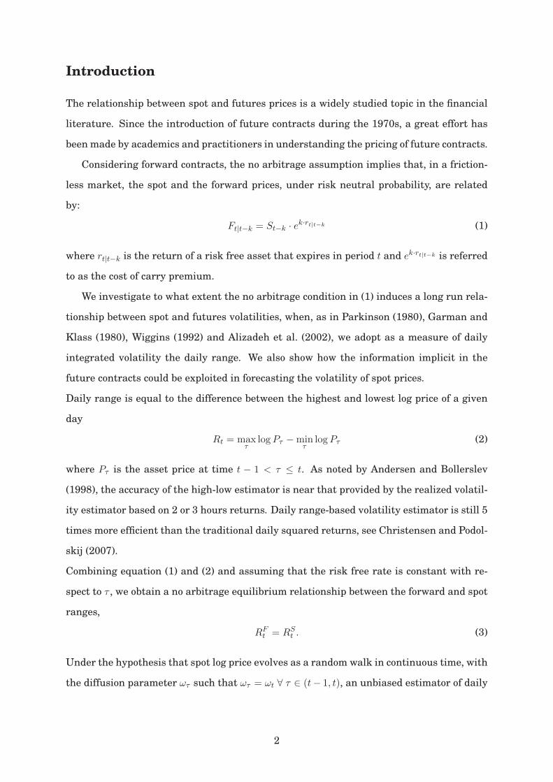
Table 8: Table reports the median (Q50), the 5th (Q5) and 95th (Q95) percentile of estimators

d, b, β and α for T = 2000, 1000, 500 observations. In the simulation, d = 0.4, α = (−0.5, 0.5)and β = −1. The values of b used in the Monte Carlo are reported.

29

T 2000 1000 500

b 0.3 0.4 0.3 0.4 0.3 0.4

Q50,d 0.4017 0.4011 0.4016 0.4004 0.4044 0.4010

Q5,d 0.3750 0.3659 0.3533 0.3505 0.3288 0.3327

Q95,d 0.4286 0.4351 0.4470 0.4498 0.4700 0.4677

RMSE 0.0162 0.0215 0.0292 0.0301 0.0426 0.0414

Q50,b 0.3007 0.4022 0.3071 0.4089 0.3224 0.4137

Q5,b 0.1980 0.3005 0.1255 0.2577 0.0344 0.1647

Q95,b 0.3874 0.5102 0.4966 0.5598 0.5839 0.6329

RMSE 0.0570 0.0617 0.1111 0.0912 0.1747 0.1418

Q50,β −0.9992 −1.0005 −1.0012 −1.0003 −0.9984 −1.0001

Q5,β −1.0184 −1.0165 −1.0401 −1.0243 −1.0611 −1.0362

Q95,β −0.9790 −0.9843 −0.9644 −0.9777 −0.9416 −0.9650

RMSE 0.0118 0.0096 0.0233 0.01409 0.0374 0.0223

Q50,α1−0.5077 −0.5037 −0.4983 −0.4995 −0.4575 −0.4693

Q5,α1−0.9109 −0.8899 −1.4939 −1.0717 −2.5199 −1.5050

Q95,α1−0.2135 −0.1942 0.0223 −0.0982 0.4741 0.0560

RMSE 0.2081 0.1964 0.4619 0.3123 0.9924 0.4671

Q50,α20.5098 0.4992 0.4914 0.4845 0.4467 0.4999

Q5,α20.2182 0.1942 −0.0282 0.0897 −0.3841 −0.0522

Q95,α20.9275 0.8407 1.5519 1.0320 2.5715 1.4114

RMSE 0.2114 0.1946 0.4839 0.3171 0.9318 0.4359

Table 9: Table reports the median (Q50), the 5th (Q5) and 95th (Q95) percentile of estimators

d, b, β and α for T = 2000, 1000, 500 observations with constant conditional correlation

errors. In the simulation, d = 0.4, α = (−0.5, 0.5) and β = −1. The values of b used in the

Monte Carlo are reported.

30

Figure 1: Autocorrelogram of log σt,F and log σt,S .

31

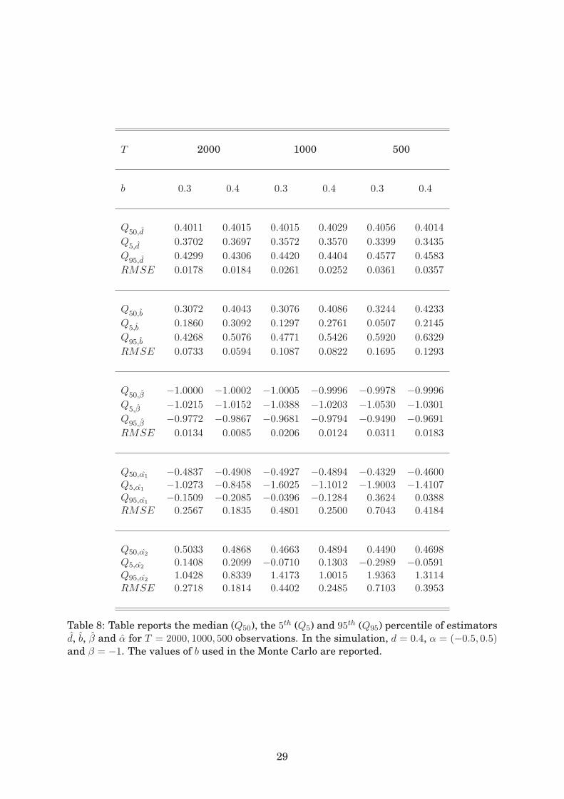
Figure 2: Error Correction Term: Figure plots the error term given by log(σFt )+ β log(σF

t ). The fractional integration order of the error term,

estimated with the exact local Whittle estimator, is equal to 0.0007.

32

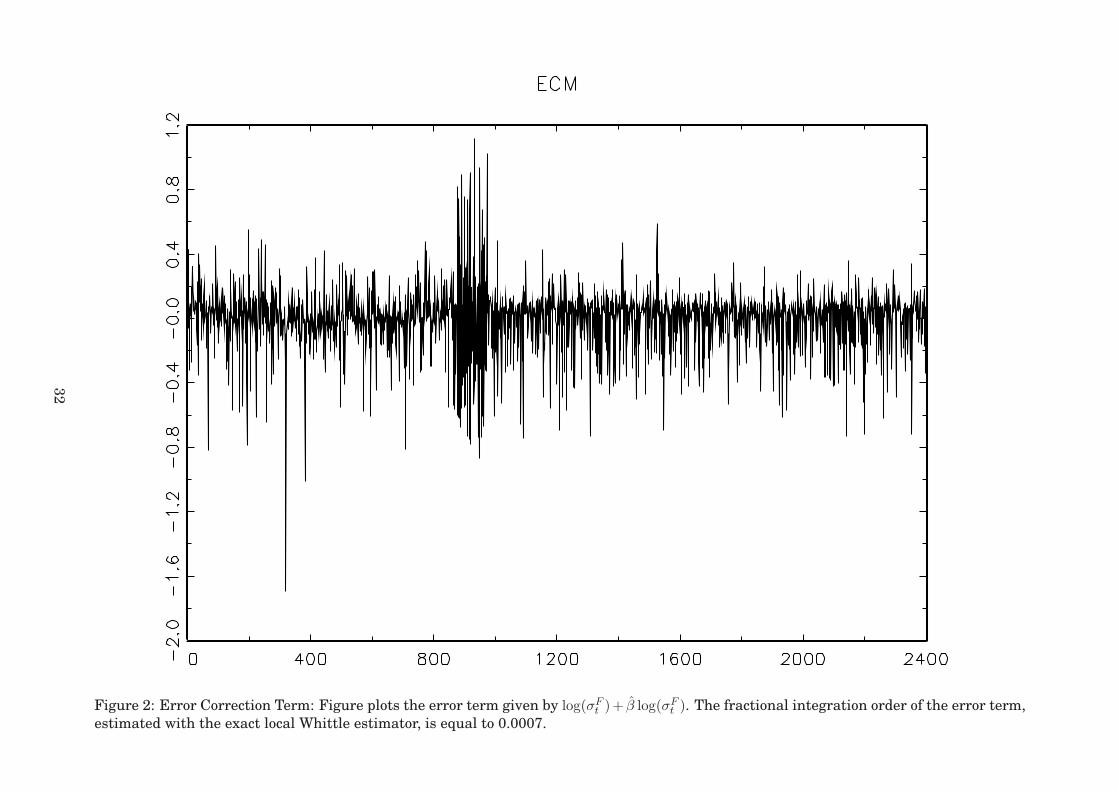
Figure 3: Kernel Densities of β, α and b.

33

(a) Panel A, b = 0.3 (b) Panel B, b = 0.3 with GARCH

(c) Panel C, b = 0.4 (d) Panel D, b = 0.4 with GARCH

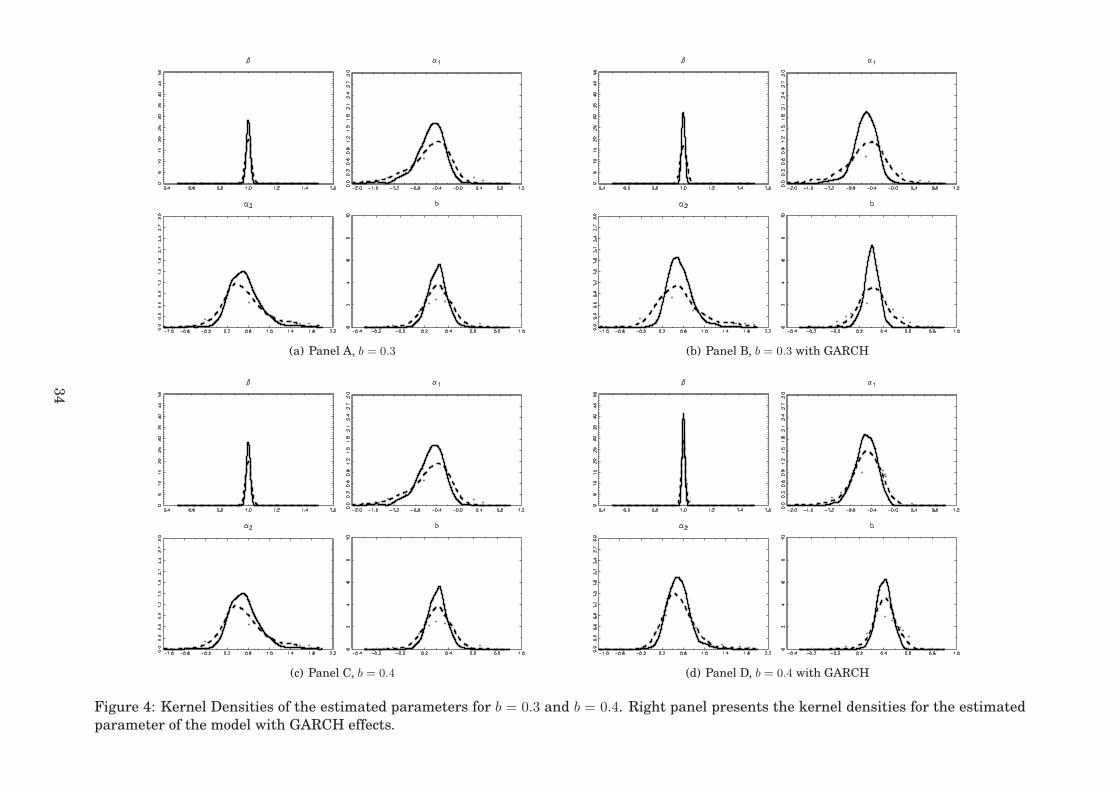
Figure 4: Kernel Densities of the estimated parameters for b = 0.3 and b = 0.4. Right panel presents the kernel densities for the estimated

parameter of the model with GARCH effects.

34

Research Papers 2009

2009-17: Tom Engsted: Statistical vs. Economic Significance in Economics and

Econometrics: Further comments on McCloskey & Ziliak

2009-18: Anders Bredahl Kock: Forecasting with Universal Approximators and a Learning Algorithm

2009-19: Søren Johansen and Anders Rygh Swensen: On a numerical and graphical technique for evaluating some models involving rational expectations

2009-20: Almut E. D. Veraart and Luitgard A. M. Veraart: Stochastic volatility and stochastic leverage

2009-21: Ole E. Barndorff-Nielsen, José Manuel Corcuera and Mark Podolskij: Multipower Variation for Brownian Semistationary Processes

2009-22: Giuseppe Cavaliere, Anders Rahbek and A.M.Robert Taylor: Co-integration Rank Testing under Conditional Heteroskedasticity

2009-23: Michael Frömmel and Robinson Kruse: Interest rate convergence in the EMS prior to European Monetary Union

2009-24: Dominique Guégan: A Meta-Distribution for Non-Stationary Samples

2009-25: Ole E. Barndorff-Nielsen and Almut E. D. Veraart: Stochastic volatility of volatility in continuous time

2009-26: Tim Bollerslev and Viktor Todorov: Tails, Fears and Risk Premia

2009-27: Kim Christensen, Roel Oomen and Mark Podolskij: Realised Quantile-Based Estimation of the Integrated Variance

2009-28: Takamitsu Kurita, Heino Bohn Nielsen and Anders Rahbek: An I(2) Cointegration Model with Piecewise Linear Trends: Likelihood Analysis and Application

2009-29: Martin M. Andreasen: Stochastic Volatility and DSGE Models

2009-30: Eduardo Rossi and Paolo Santucci de Magistris: Long Memory and Tail dependence in Trading Volume and Volatility

2009-31: Eduardo Rossi and Paolo Santucci de Magistris: A No Arbitrage Fractional Cointegration Analysis Of The Range Based Volatility


Recommended