Page 1
Creation of a water market in the Athabasca oil sands region: will vertical
integration create incentives for entry deterrence?
by
Krista Predy
A thesis submitted in partial fulfillment of the requirements for the degree of
Master of Business Administration
Faculty of Business
University of Alberta
© Krista Predy, 2015
Page 2
ii
Abstract
The implications of creating a water market in the Athabasca region of Northern Alberta are
examined with the objective of creating a system which encourages efficient water usage by oil
sands mining producers. An analysis is performed considering entry to the oil industry when
there is no constraint on available water supply versus a situation where the available water
supply is constrained. Vertically integrated incumbent oil firms can strategically increase their
capacity investment in the downstream oil market to exercise market power in the upstream
water market, resulting in entry deterrence when there is a constraint on the water supply. In the
absence of a constraint on the water supply, we show that the market will be no more efficient
than the current water allocation system.
Page 3
iii
Table of Contents
Abstract ........................................................................................................................................... ii
I. Introduction ............................................................................................................................. 1
I. Background .............................................................................................................................. 4
II. Model ....................................................................................................................................... 8
Case 1: The static model without entry ....................................................................................... 8
Case 2: The case with slack water quotas ................................................................................. 12
Case 3: Accommodation ........................................................................................................... 14
Case 4: Entry deterrence ........................................................................................................... 15
III. Example ............................................................................................................................. 16
IV. Discussion .......................................................................................................................... 17
V. Conclusion ............................................................................................................................. 22
Bibliography ................................................................................................................................. 24
VI. Appendix ............................................................................................................................ 26
List of Tables and Charts
Chart 1………………………………………………………………………………………….. 6
Table 1………………………………………………………………………………………….. 17
Page 4
1
I. Introduction
The oil sands in Northern Alberta, Canada are among the largest proven oil reserves in the world.
These deposits are unconventional oil, rather than traditional crude oil. The extraction of these
unconventional oil reserves via mining is far more water intensive than traditional crude oil. In
fact, the sole source of water for oil sands mining is fresh water, used at an average rate of 2.5
barrels of fresh water per barrel of oil produced. Total oil sands production used over 1.2 billion
barrels of water in 2013 to produce 0.7 billion barrels of oil (Alberta Environment and
Sustainable Resource Development, 2014). According to the Pembina Institute, the total oil
sands water usage in 2011 would be equivalent to the annual residential water use of 1.7 million
Canadians. Aside from a one-time application fee for a water licence and any related water
infrastructure cost specific to the operation, water is effectively a free commodity for use in the
oil production process. This would suggest that there is potential for overuse of an essentially
free input to the production process. This thesis examines the benefits and consequences of
setting up a water market in the Athabasca region.
The following analysis will focus on oil sands mining operations which are massive in scale.
According to the Government of Alberta, there were 114 active oil sands projects in 2013, with 6
of these projects being mining operations. Imperial Oil’s Kearl mine is not yet considered fully
operational, but is one example of the massive scale of this type of project. The Kearl project has
a $12.9 billion dollar price tag and its expected capacity is 40 million barrels per year (Lewis,
2014); the project has a water allocation equivalent to over 600 million barrels of water per year
(Alberta Environment and Sustainable Resource Development, 2014). These oil sands mining
projects are large scale operations which yield a massive capital cost and are challenged with
selling their oil at market prices. Given the current mining technology and the scale of these
projects, we see that water is an integral component to the production of oil: the resulting
production function faced by the oil producers is increasing in both capital investment and in
water. This suggests that water and capital are complementary inputs to the production process.
Page 5
2
We conjecture that in such a scenario, and with the introduction of a water market, capital
investment may be used to drive up the resultant water price in order to deter entry.
Early literature in strategic entry deterrence by Dixit (1979) and Spence (1977) found that
investment in capacity by a monopolist can be used to deter entry as it creates a credible threat to
the entrant’s future profits. Gilbert and Vives (1986) extended the analysis to multiple, non-
cooperating, incumbent firms to find that it can still be profitable for these firms to invest in
capacity to deter entry, provided the entrant faces a fixed cost, or entry cost. To operate a mining
project, the oil producers must invest in large amounts of capital, and these large-scale capital
projects require a correspondingly large water allocation to accommodate the high volume of
production. The distinction is that this scenario, unlike the classic models of entry deterrence,
includes oil firms who operate as price takers in the oil market and thus have no ability to
directly impact entrants’ profits in this market. The model proposed in this paper is constructed
to examine the impact of the creation of an upstream water market which causes these firms to
become vertically integrated.
Vertical integration has long been a topic of economic debate as to whether integration creates
efficiencies or whether it restricts competition. Kuhn and Vives (1999) looked at the welfare
impact of vertical integration of an upstream monopolist when the downstream industry is
imperfectly competitive. They show that vertical integration actually increases output
downstream, due to cost efficiencies from eliminating double marginalization; however they
neglect to consider any potential strategic effects on the market. Salinger (1988) found that an
upstream monopolist can limit access to the upstream input, if vertical integration results in
market foreclosure; this will cause a resultant price increase in the downstream market. De
Fontenay and Gans (2005), however, show that there is a greater incentive for vertical integration
under upstream competition than under upstream monopoly, thus competition enhances the
potential for strategic vertical integration. Normann (2011), found empirical evidence that
supports the hypothesis that markets containing vertically integrated firms are less competitive
and when the vertically integrated firm is present, prices will generally be higher than in non-
Page 6
3
integrated industries. Our model examines whether the creation of a vertically integrated set of
incumbent oil firms will in fact be more efficient, regarding water usage and cost minimization
or whether the firms will use the fact that capital investment and water usage are complements to
deter entry.
To our knowledge this type of analysis has not yet been applied to the oil and gas sector. The
current literature on vertical integration focuses on the exercise of market power in the
downstream market which can be identified as an increase in the downstream price. Our paper is
unique in that, as far as we can find, it is the first paper to suggest that the vertically integrated
firms may exercise market power in the upstream market, not the downstream market. The oil
firms can overinvest in capital (hereafter stated as the capacity) downstream to strategically
manipulate the upstream market due to the complementarily of capacity and water. We will show
that the companies can credibly increase their capacity, thereby increasing their water demand to
the point where they have used up their entire water allocation, resulting in an increase in the
water price upstream.
Advocates for water policy reform in Alberta have promoted the creation of a water market to
stimulate efficient use of water and to reduce waste. Percy (2005) advocated a market based
approach to water allocation as a potential solution to scarcity. However, adoption of a water
market in Northern Alberta may result in a market that does not function effectively; the fact that
there are few players in the region raises questions about the potential for a viable market in
terms of facilitating water exchanges and transfers (Adamowicz, Percy, & Weber, 2010).
The absence of an efficient water market currently exists in southern Alberta, where transfers of
allocations between water licensees have been allowed for over a decade. These transfers may
take one of two forms: temporary transfers do not require any official approval by the
government, while permanent transfers of water rights are approved by the regulator. The price
which changes hands for either type of transaction, however, is not determined by the market;
the price is privately agreed to between the buyer and seller. Although market proponents may
think that allowing water transfers will facilitate more efficient use of water, the ‘market’ has
Page 7
4
produced a different result: since the allowance of transfers, very few transfers have actually
taken place. Despite publically searching for a purchasable water allocation, the town of
Okotoks, Alberta had to undergo water rationing, over a period population growth, for several
years. The municipality was finally able to acquire an additional water allocation in 2013.
(Patterson, 2013). A possible explanation for the lack of activity in this market is that about 75%
of the water licenses in the South Saskatchewan River Basin are for irrigation or agriculture
purposes. The vast majority of these licenses are controlled by associations called irrigation
districts – these districts have rules whereby the district has to approve the transfer of a water
license held by a member. Market power of the irrigation districts is a likely reason why few
water market transactions have taken place to date in Southern Alberta. The market power seen
in southern Alberta is not unlike the potential market power the oil producers would hold in the
north under a water market.
The remainder of this thesis will be organized as follows: Section II will provide a background
on the oil sands operations, the production and current water licensing, and usage in the region.
Section III will define the model and describe the results for the case where there is no entry in
the market, which results in an efficient market outcome where price equals marginal cost; it will
then go on to discuss the case where there may be entry in the market. The findings here are that,
in the absence of a binding constraint on water supply, accommodation will be optimal whereas
if the water supply constraint is binding, it may be optimal for firms to deter entry. Section IV
will provide a brief numerical example. Section V is a discussion of the findings and section VI
will conclude the paper.
I. Background
The majority of oil sands activities (and all oil sands mining activity) takes place in the
Athabasca watershed, located in northern Alberta, which is home to the Athabasca River. Flows
from the Athabasca River originate in the Rocky Mountains and the river flows east through the
northern part of the province, eventually emptying into the Peace-Athabasca delta in the North
Page 8
5
Eastern Alberta. As of 2010, about seventy-five percent of the water allocations from the
Athabasca River Basin were for industrial purposes, the vast majority of which are used for the
purposes of bitumen mining near Fort McMurray, Alberta (Alberta Environment, 2010). Other
remaining water allocations for commercial and municipal purposes are comparatively small and
are dispersed along the length of the Athabasca River.
The Athabasca River is fed by the Columbia Glacier and as such it experiences significant
fluctuations in seasonal flows. The flows in the spring and summer, when the snow melts and
runs off, are typically five to six times greater than the winter flows when the river is frozen over
(Environment Canada, 2014). Schindler and Donahue (2006) caution that climate warming
trends show potential for significantly decreased river flows in the Prairie Provinces in the
future. Although the current river flows are adequate to meet the needs of the water users in the
area, potential growth in population and industry activity, along with decreased flows indicates
that water constraint is a strong possibility in the future.
There are currently two different technologies being employed in the recovery of oil, or more
specifically bitumen, from the oil sands: mining and in-situ technology. In 2013, mining
activities accounted for nearly fifty-five percent of all oil production from the oil sands. Mining
activities, however, consumed almost ninety percent of the total fresh water used in the
extraction and upgrading of bitumen from the oil sands, while in-situ recovery projects used just
over ten percent (Alberta Environment and Sustainable Resource Development, 2014). Although
the area and absolute quantity of oil sands reserves are very large, much of the known reserves
are not fully recoverable with the current available technology. Mineable reserves account for
less than 10% of the total reserves but are estimated to make up over one-fifth of the recoverable
total (Griffiths, Taylor, & Woynillowicz, 2006). Mining activities have been the predominant
method of oil sands extraction for the past five decades. Although production through in-situ
technology is growing rapidly, the Canadian Association of Petroleum Producers is forecasting
the annual volume of mining production to nearly double over the next 15 years.
Page 9
6
Chart 1:
1. Production mining forecast taken from CAPP’s June 2014 release
2. Average water usage per barrel from GOA oil sands information portal, 2013 data
The above graph demonstrates a dramatically increasing demand for water in mining operations
over the next 15 years, and the primary source of this water will be from the Athabasca River.
Although the water allocations currently outstanding to the existing oil producers will be
sufficient to satisfy this projected demand, there are still potential constraints. This projection is
based on currently planned operations and their expected future output; entry to the industry
could place further demands on the water supply. Also it is possible that drought or climate
change may cause shocks to the future expected water supply in the area. Forward looking firms
will realize potential water scarcity could threaten their future profitability and may find it in
their best interest to act strategically.
The current legislation does not allow for in-situ operations to get licenses for water withdrawals
from any major rivers – they are restricted to using water mainly from groundwater (aquifers)
and some from surface water/runoff. As per Alberta Energy Regulator’s Directive 81 (2012), in-
situ operators are subject to stringent guidelines regarding water recycling and usage rates that
are mandatory for their operations; no analogous legislation exists regarding mandatory
recycling rates for mining operations.
0
400
800
1,200
1,600
2013 2015 2017 2019 2021 2023 2025 2027 2029
Mil
lion
s of
Barr
els
per
yea
r
Oil Sands Mining Production and Water Usage Forecast 1,2
Oil Sands Mining Production Water needed for Mining
Page 10
7
Oil sands mines face no mandatory recycling rate or regulation on the efficiency of their
operations regarding the volume of water used per barrel of oil produced. Mining operations
used a total of 164 million m3 of water in 2013, most of which is from the Athabasca River
(Alberta Environment and Sustainable Resource Development, 2014). There are currently five
firms with approved or operating oil sands mining operations, as of November 2014 (Alberta
Environment and Sustainable Resource Development, 2014) and these five firms hold close to
75% of the industrial water allocations from the Athabasca. As previously mentioned, the mining
industry is characterized by entry and exit of firms: Imperial Oil is one of the five firms which
have recently entered that market, following Canadian Natural Resources in 2008 and Shell in
2002. Both Suncor and Syncrude are established market leaders and have been operating their oil
sands mines since 1967 and 1978, respectively. In contrast to this, there are around 30 different
companies with operational in-situ projects, and many more companies with proposed and
approved in-situ projects, indicating that these operations have a different scale and less market
power than the mining operations. Given that in-situ production is far less water intensive, we
have focused our model on water usage from mining operations only.
The northern part of Alberta is sparsely populated and the main industrial activity in the area is
oil and gas. In earlier years, the industry’s contribution to the economy was welcomed, but a
recent period of rapid growth in production and the number of projects has many criticizing the
environmental footprint of these industrial activities. There is a large First Nation population in
the northern part of the province who historically survived by hunting and fishing, and uses the
Athabasca River as their main source of transportation. Increasing pollution levels in the
Athabasca River are correlated to increasing water usage by the industry (Jasechko, Gibson,
Birks, & Yi, 2012). This is of concern, especially to the First Nations who use the river as a food
source and for their livelihood. For the purpose of this paper, we chose to focus only on the
strategic impact of water usage. However creation of a mechanism to incorporate the cost of
pollution to the environment and to society into the water price is one area for future research.
Page 11
8
For the model, we section the water users in the Athabasca watershed region into three groups:
the local community, the First Nations community, and the oil producers. Each group is assumed
to be grandfathered into the market with an initial endowment equal to the amount of water
allocated to them under the current licensing system. Under the market these three groups are
assumed to hold the total regional water supply which they are then able to sell to each other or
to new demanders of water. The First Nations communities in Canada are governed by slightly
different regulations, which are federal and not provincial, and as such they do not actually hold
any water licenses. However the Constitution Act of 1982 does protect Aboriginal rights to
Aboriginal title, which includes traditional and new economic uses of water (Walkem, 2007).
Therefore, although these rights are not explicitly licensed, our model recognizes that the First
Nations in the Fort McMurray, Fort Chipewyan and surrounding areas do have a claim to water
rights. Under the water market model, the First Nations are assumed to be grandfathered into the
market with an initial endowment equal to their current water utilization.
II. Model
Consider an economy with consumers and suppliers of water, operating in an upstream water
market, including oil producing firms. Vertically integrated oil firms then use the water as an
input to produce oil in the downstream market. The following model consists of four stages:
Stages 1 and 2 are based on a Stackelberg leader-follower model, where the incumbent oil
producers make their choice of capacity in stage 1 and a potential entrant makes his choice of
capacity (and entry) in stage 2. In stage 3, water suppliers choose the quantities of water to
supply the market, based on a Cournot framework. In stage 4 we derive the water demands for
the consumers, to find the producer demand function, which gives the water price as a function
of the quantity demanded.
Case 1: The static model without entry
We begin by deriving the water demand of consumers, which is stage 4. There are 𝑛1 final
consumers from the local community and 𝑛2 final consumers from the First Nation, who
Page 12
9
consume water and a basket of consumer goods. These final consumers choose their water
demand 𝑎𝑖 to maximize the objective function: 𝑣𝑖 = 𝑥𝑖 + 𝑎𝑖(𝑏 − 𝑎𝑖2
) − 𝑝𝑎𝑖 where the second
term denotes the benefits derived from water consumption and 𝑥𝑖 is the net benefit from
consumption of all other consumer goods. Note that 𝑝 is the water price and b is a constant,
which represents the consumer’s maximal willingness to pay for water.
There are also intermediate consumers of water who use the water as an input to some
production process. There are 𝑛2 intermediate First Nation consumers who use water for
transportation, fishing, etc. and 𝐽 intermediate consumers who use the water as an input to the oil
production process. The first nations choose 𝑎𝑓 to maximize their production function, given
by 𝑎𝑓 (𝛾 − 𝑎𝑓
2) − 𝑝𝑎𝑓, where 𝛾 is a positive constant. Each oil producer chooses 𝑎𝑜to maximize
its profit function, given by 𝑒(𝑎𝑜; 𝑘𝑗) − 𝑝𝑎𝑜 − 𝑘𝑗𝑟 − 𝐹, where 𝑒(𝑎𝑜; 𝑘𝑗) denotes the firm’s
energy production function, 𝑘𝑗 is the amount of capital (i.e., capacity), r is the price per unit of
capacity and F is a fixed cost. We assume that 𝑒(𝑎𝑜; 𝑘𝑗) = 𝑎𝑜 (𝑠 −𝑎𝑜
2) + 𝑘𝑗(𝑧 − 𝑘𝑗) + 𝑎𝑜𝑘𝑗,
where 𝑠 and 𝑧 are positive constants which represent the maximal marginal products of water
and capacity, respectively. We also assume that the price of energy is equal to 1.
Each individual in any group will choose to consume water to maximize his or her respective
objective function, leading to choices that equate marginal benefits from consumption of water to
the marginal costs of doing so. Assuming interior solutions, the marginal conditions are formally
expressed as follows:
(1.1) Final Consumers: 𝑏 − 𝑎𝑖 − 𝑝 = 0
(1.2) First Nation (intermediate): 𝛾 − 𝑎𝑓 − 𝑝 = 0
(1.3) Oil Companies: 𝑠 + 𝑘𝑗 − 𝑎𝑜 − 𝑝 = 0
We assume that 𝑝 < min {𝑏, 𝛾, 𝑠}. Solving first order conditions (1.1) to (1.3) yields the water
demand function for each of the groups, which are linear and decreasing in price. Equation (1.3)
reveals that capacity 𝑘𝑗 is a strategic complement to water. This implies that the water demand
Page 13
10
for the oil producers is stated as an increasing linear function of capacity as well as being a
function of price.
Let 𝑄 = 𝑄𝑜 + 𝑄𝑓 + 𝑄𝑙 denote the total quantity of water supplied in the market, where 𝑄𝑜 , 𝑄𝑓 ,
and 𝑄𝑙 are the total quantities supplied by the oil industry, the first nation and the local
community, respectively. Adding up the total water demands for all consumers from 1.1 to 1.3,
we obtain the market clearing condition for the water market: 𝑄 = 𝑏𝑛𝑅 + 𝑛2𝛾 + 𝐽𝑠 + 𝐾𝐼 −
𝑝(𝑛𝑅 + 𝑛2 + 𝐽). Solving for the water price, we have:
𝑝(𝑄, 𝐾𝐼) =𝑛𝑅𝑏 + 𝑛2𝛾 + 𝐽𝑠 + 𝐾𝐼 − 𝑄
𝑁,
that is, the inverse water market demand function, where 𝑁 = 𝑛𝑅 + 𝑛2 + 𝐽 for 𝑛𝑅 = 𝑛1 + 𝑛2
and 𝐾𝐼 = ∑ 𝑘𝑗𝐽1 .
Stage 3: The water endowments (quotas) are Y𝑜 for the oil companies, Y𝑓 for the First Nation
and Y𝑙 for the local community. The total available water supply is given by 𝑌 = Y𝑙 + Y𝑓 + Y𝑜.
We assume that the water endowment for each group is greater than the sum of their marginal
willingness to pay:
Y𝑙 > 𝑛1𝑏, Y𝑓 > 𝑛2(𝛾 + 𝑏), Y𝑜 > 𝐽𝑠
As we will demonstrate below, these conditions ensure that the water quotas do not bind in a
static model where there is no entry in the oil and gas industry. This is a modeling strategy. It
allows us to consider a case in which the water quota constraint for the oil producer binds when
there is potential entry. We will show that a binding water quota constraint for the oil industry is
a necessary condition for incumbents to have incentives to strategically deter entry.
a. Oil producers choose 𝑞𝑗𝑜 ∈ (0, 𝑦𝑜) to maximize Π𝑗 , where 𝑄𝑜 = ∑ 𝑞𝑗
𝑜𝐽1 𝑎𝑛𝑑 𝑌𝑜 = ∑ 𝑦𝑜𝐽
1
(3.1) Π𝑗 = (𝑝 − 𝑐)𝑞𝑗𝑜 + 𝑎𝑜 (𝑠 −
𝑎𝑜
2) + 𝑘𝑗(𝑧 − 𝑘𝑗) + 𝑎𝑜𝑘𝑗 − 𝑝𝑎𝑜 − 𝑘𝑗𝑟 − 𝐹
We assume that 𝑧 > 𝑟.
b. The local government choose 𝑄𝑙 ∈ (0, 𝑌𝑙) to maximize:
(2)
Page 14
11
(3.2) 𝛱𝑙 = (𝑝 − 𝑐)𝑄𝑙 + 𝐽Π𝑗 +𝑛1
2(𝑏 − 𝑝)2
c. The First Nations government chooses 𝑄𝑓 ∈ (0, 𝑌𝑓) to maximize:
(3.3) 𝛱𝑓 = (𝑝 − 𝑐)𝑄𝑓 +𝑛2
2(𝛾 − 𝑝)2 +
𝑛2
2(𝑏 − 𝑝)2
The profits for each group (equations (3.1) to (3.3) above) include the profits earned from the
sale of water: when price equals the marginal cost of water, there will be zero contribution to
profits from the sale of water. However, when the price of water is greater than the marginal
cost, each group will find it profitable to sell water as they gain a profit of 𝑝 − 𝑐 for each unit of
water sold. The remaining terms in the profit functions denote the revenues/benefits from using
water, less the cost incurred, measured in terms of consumer surplus foregone.
Assuming interior solutions, the optimization problems yield the following first order conditions:
(4.1) (𝑝 − 𝑐) + [𝑞𝑗𝑜 − 𝑎𝑜(𝑝, 𝑘𝑗)]
𝑑𝑝
𝑑𝑄= 0
(4.2) (𝑝 − 𝑐) + [𝑄𝑙 − 𝑛1𝑎𝑖(𝑝)]𝑑𝑝
𝑑𝑄= 0
(4.3) (𝑝 − 𝑐) + [𝑄𝑓 − 𝑛2𝑎𝑓(𝑝) − 𝑛2𝑎𝑖(𝑝)]𝑑𝑝
𝑑𝑄= 0
Solving for the groups’ total water supplies, we obtain the water supply, given as follows:
(5.1) 𝑄𝑜 = 𝐽𝑠 + 𝐾𝐼 − 𝐽𝑁𝑐 + (𝑁 − 1)𝐽𝑝
(5.2) 𝑄𝑓 = 𝑛2(𝛾 + 𝑏) − Nc + p(𝑁 − 2𝑛2)
(5.3) 𝑄𝑙 = 𝑛1𝑏 − 𝑁𝑐 + 𝑝(𝑁 − 𝑛1)
Adding up (5.1) to (5.3) yields
(6) 𝑄 = 𝑛𝑅𝑏 + 𝑛2𝛾 + 𝐽𝑠 + 𝐾𝐼 − 𝑁𝑐(𝐽 + 2) + 𝑝𝑁(𝐽 + 1)
Using the producer demand function (equation 2) derived in stage 4, this can be solved for price
to get 𝑝∗ = 𝑐. This indicates that the water market is efficient and competitive, as none of the
users has the desire to buy or sell more water than is required to meet their own needs since we
have obtained a price equal to marginal cost in equilibrium. The complementarity of water and
Page 15
12
capacity here will have no impact on the downstream market; although 𝐾𝐼 appears in the supply
function (6) and in the producer demand function (2), the two cancel out in equilibrium, resulting
in a water price that is not dependent on the choice of capacity. Thus, in the absence of entry into
the market, vertical integration will have no impact on the equilibrium outcome in the
downstream market as oil producers will use water at the same cost as they do under the current
system since 𝑝∗ = 𝑐.
Entry in the oil and gas industry
The model of the previous section assumes that there is no entry in the oil and gas industry. We
now consider a situation where there is potential entry into the oil and gas industry. The only
difference with respect to the previous model is that the entrant’s water demand must be included
in the derivation of the producer demand function as he will need water to enter the oil market.
The entrant will be denoted by the subscript 𝐽 + 1 and the water demand for the entrant will have
the same form as for the incumbents: 𝑎𝑜(𝑝; 𝑘𝐽+1) = 𝑠 + 𝑘𝐽+1 − 𝑝.
Case 2: The case with slack water quotas
Consider the case where there is an entrant and the water quotas are not binding (as we assumed
with the choice of quantities above). Here we obtain the following inverse demand function:
𝑝 =𝑛𝑅𝑏 + 𝑛2𝛾 + (𝐽 + 1)𝑠 + 𝐾𝐼 + 𝑘𝐽+1 − 𝑄
𝑁 + 1
Suppliers choose their quantities to supply as above, only now they take into account the demand
of the entrant when choosing a quantity to supply. The outcome of stage 3 is that the entry drives
up the water price so that 𝑝 > 𝑐, resulting in the following function for the water price:
𝑝 = [𝑠 + 𝑘𝐽+1 + (𝐽 + 2)(𝑁 + 1)𝑐
𝐽𝑁 + 2𝑁 + 𝐽 + 3]
Due to the complementarity of water and capacity, the price is dependent on the entrant’s choice
of capacity and will increase with scale of entry. The price is again not dependent on the
(7)
Page 16
13
incumbent producer’s choice of capacity, indicating that choice of capacity is not strategic for
the incumbents.
In stage 2, the entrant will choose capacity 𝑘𝐽+1to maximize Π𝐽+1:
Π𝐽+1(𝑝, 𝑘𝐽+1) =𝑎𝑜(𝑝, 𝑘𝐽+1)
2
2+ 𝑘𝐽+1(𝑧 − 𝑟 − 𝑘𝐽+1) − 𝐹
(8.1) First order conditions: 𝑠 − 𝑘𝐽+1 − 𝑝 + 𝑧 − 𝑟 + (𝑝 − 𝑠 − 𝑘𝐽+1)𝑑𝑝
𝑑𝐾= 0
In stage 1, the incumbents will choose capacity 𝑘𝑗 to maximize Π𝑗:
Π𝑗(𝑝, 𝑞𝑗𝑜 , 𝑘𝑗) = (𝑝 − 𝑐)𝑞𝑗
𝑜 +𝑎𝑜(𝑝, 𝑘𝑗)
2
2+ 𝑘𝑗(𝑧 − 𝑟 − 𝑘𝑗) − 𝐹
(8.2) First Order condition: 𝑠 − 𝑘𝑗 − 𝑝 + 𝑧 − 𝑟 + (𝑞𝑗𝑜 − 𝑠 − 𝑘𝑗 + 𝑝)
𝑑𝑝
𝑑𝐾= 0
In fact, the choice of capacity 𝑘𝑗 by the incumbents is the same as in the case where there is no
entry into the industry. When the water allocations given to the industry are not binding, the
incumbent firms have no incentive to deter entry to the market. This result is surprising as it
indicates that, in the absence of a binding constraint on the water supply, the incumbents are
actually better off by allowing entry and earning additional profits from the sale of water.
The cases when the oil industry’s water quota binds
Now we consider the case where there is a binding constraint on the water supply. We look at the
case 𝑄𝑜 = 𝑌𝑜, where the oil producers wish to supply more water in the market than they have
available. The incumbent oil firms are able to deter entry to the industry, provided that their
water constraint is binding (𝑄𝑜 = 𝑌𝑜). As we will discuss in the section v, this creates the
necessary condition that will make the water price dependent on the incumbent producers’
choice of 𝑘𝑗. For simplicity, we will just examine the least restrictive case where the only
suppliers facing a supply constraint are the oil firms, however all cases have been calculated in
the appendix.
Page 17
14
Let Q = 𝑌𝑜 + 𝑄𝑙 + 𝑄𝑓, so that only the oil firms face a binding constraint on the water supply.
There are two possible outcomes: accommodation and deterrence. Although it is possible for the
incumbents to deter entry when the water supply is limited by water availability, we will
examine the payoffs between the cases where an entrant is allowed into the market versus when
they are deterred.
Case 3: Accommodation
Accommodation is analyzed first. The same first order conditions are used to derive the water
demands in stage 4. As before, water demand can be stated as a function of price, only here, it
becomes a function of 𝑌𝑜, not 𝑄𝑜:
𝑝 =𝑛𝑅𝑏 + 𝑛2𝛾 + (𝐽 + 1)𝑠 + 𝐾𝐼 + 𝑘𝐽+1 − 𝑌𝑜 − 𝑄𝑙 − 𝑄𝑓
𝑁 + 1
Since the water quota 𝑌𝑜 here is fixed, the price function is now dependent on the capacity
choices of the oil producers. This can be seen after stage 3 when we can simplify the price to:
𝑝 =(𝐽 + 1)𝑠 + 𝐾𝐼 + 𝑘𝐽+1 − 𝑌𝑜 + 2(N + 1)c
2𝑁 + 𝐽 + 3
We saw in the prior cases that the choice of water quantity was dependent on the incumbent’s
capacity, but the capacity reduced out of the price function when we solved for the quantities,
resulting in a price and was not dependent on the capacity choice. When the water demand
exceeds the supply, the choice of price becomes strategic, as the function for price is increasing
in capacity. Thus the incumbent producers can select a higher 𝐾𝐼 to drive up the water price.
As before, when there was no constraint on the water supply, the entrant will choose capacity to
maximize profits Π𝐽+1, subject to this revised producer demand function (10) and the first order
conditions (8.1). The incumbents choose capacity to maximize Π𝑗 , according to the same first
order conditions as before (8.2), subject to the above price function (10) to obtain:
(10)
(9)
Page 18
15
𝐾𝐼𝐴𝑐𝑐𝑜𝑚 =
(2𝑁 + 𝐽 + 3)[(2𝑁 + 𝐽 + 2)𝐽𝑠 + (2𝑁 + 𝐽 + 3)𝐽(𝑧 − 𝑟)]
((2𝑁 + 𝐽 + 3)(2𝑁 + 𝐽 + 4) + (𝐽 + 1)(2𝑁 + 𝐽 + 2))
+((2𝑁 + 𝐽 + 3)(2𝑁 + 𝐽 + 4) + (2𝑁 + 𝐽 + 2))𝑌𝑜
((2𝑁 + 𝐽 + 3)(2𝑁 + 𝐽 + 4) + (𝐽 + 1)(2𝑁 + 𝐽 + 2))(2𝑁 + 𝐽 + 4)
−(2𝑁 + 𝐽 + 2)𝐽[(𝐽 + 1)𝑠 − 𝑌𝑜 + 2(N + 1)c]
((2𝑁 + 𝐽 + 3)(2𝑁 + 𝐽 + 4) + (𝐽 + 1)(2𝑁 + 𝐽 + 2))
Water price:
𝑝𝐴𝑐𝑐𝑜𝑚 =(2𝑁 + 𝐽 + 4)[(𝐽 + 1)𝑠 − 𝑌𝑜 + 2(N + 1)c]
((2𝑁 + 𝐽 + 3)(2𝑁 + 𝐽 + 4) + (𝐽 + 1)(2𝑁 + 𝐽 + 2))
+(𝐽 + 1)[(2𝑁 + 𝐽 + 2)𝑠 + (2𝑁 + 𝐽 + 3)(𝑧 − 𝑟)]
((2𝑁 + 𝐽 + 3)(2𝑁 + 𝐽 + 4) + (𝐽 + 1)(2𝑁 + 𝐽 + 2))
+𝑌𝑜
((2𝑁 + 𝐽 + 3)(2𝑁 + 𝐽 + 4) + (𝐽 + 1)(2𝑁 + 𝐽 + 2))
Case 4: Entry deterrence
Entry deterrence will occur when the entrant cannot make positive profits in equilibrium: the
entrant will not enter the market when the incumbents choose a level of capacity 𝐾𝐼, such that
Π𝐽+1 = 0. Once again, we have the same producer demand function (9) as in the
accommodation case above where 𝑌𝑜 = 𝑄𝑜. Subject to the producer demand function (9), the
incumbents choose a higher level of capacity than they would in the case of entry, subject to:
Π𝐽+1 =𝑎𝑜(𝑝, 𝑘𝐽+1)
2
2+ 𝑘𝐽+1(𝑧 − 𝑟 − 𝑘𝐽+1) − 𝐹 = 0
Since the entrant’s profits are zero, he will not find it profitable to enter the market and we find
that the incumbent’s deterrence capacity is:
𝐾𝐼𝐷𝑒𝑡 = 𝑌𝑜 + 2(N + 1)(s − c) +
(2𝑁 + 𝐽 + 2)(𝑧 − 𝑟)
2
−((𝑧 − 𝑟)2 + 4𝛽)
12(4𝑁2 + 4𝑁𝐽 + 16𝑁 + 𝐽2 + 8𝐽 + 14)
2(2𝑁 + 𝐽 + 2)
Page 19
16
Where:
𝛽 =2(2𝑁 + 𝐽 + 2)2𝐹 − (𝑧 − 𝑟)2(2𝑁 + 𝐽 + 3)2
2(4𝑁2 + 4𝑁𝐽 + 16𝑁 + 𝐽2 + 8𝐽 + 14)
The water price becomes:
𝑝𝐷𝑒𝑡 = 𝑠 +𝑧 − 𝑟
2−
((𝑧 − 𝑟)2 + 4𝛽)12(4𝑁2 + 4𝑁𝐽 + 16𝑁 + 𝐽2 + 8𝐽 + 14)
2(2𝑁 + 𝐽 + 2)2
We find that the deterrence capacity here is higher than the accommodation capacity for the
incumbent firms. The equilibrium price is lower in the case where deterrence is optimal, since
the entrant will demand no water in equilibrium when we have deterrence. Due to the fact that
the capacity choice of the incumbents is higher under deterrence than accommodation, we can
see that the price would in fact be higher than the accommodation case should the entrant decide
to enter the market when the incumbents choose this capacity level.
We see that deterrence will only occur when there is less slack in the constraint on the water
supply: the scarcer water is for the incumbents, the more likely they are to deter entry. In
addition to this, entry deterrence requires a sufficiently large fixed cost, in the absence of a large
enough fixed cost it becomes too expensive for the incumbents to invest in a capacity level high
enough to deter entry.
III. Example
To illustrate the outcomes from the model when there is a constraint on the water supply, we
look at the following example. This example assumes that 𝐽 = 6, 𝑛1 = 200 𝑎𝑛𝑑 𝑛2 = 60. It also
assumes that 𝑐 = 2, 𝑏 = 8, 𝛾 = 12, 𝑠 = 38, 𝑧 = 840 𝑎𝑛𝑑 𝑟 = 590. We examine the effect on
capacity choice and the profits of the incumbent producers under two variations of fixed costs
and two variations of water constraint 𝑌𝑜 . The table below lists the water price, fixed cost, water
constraint, and the profit of an incumbent firm under each of 3 cases.
Page 20
17
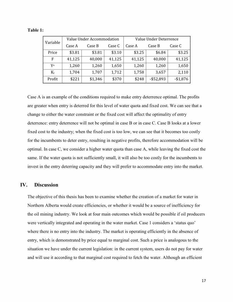
Table 1:
Variable Value Under Accommodation Value Under Deterrence
Case A Case B Case C Case A Case B Case C
Price $3.81 $3.81 $3.10 $3.25 $6.84 $3.25
F 41,125 40,000 41,125 41,125 40,000 41,125
Yo 1,260 1,260 1,650 1,260 1,260 1,650
KI 1,704 1,707 1,712 1,758 3,657 2,110
Profit $221 $1,346 $370 $248 -$52,893 -$1,876
Case A is an example of the conditions required to make entry deterrence optimal. The profits
are greater when entry is deterred for this level of water quota and fixed cost. We can see that a
change to either the water constraint or the fixed cost will affect the optimality of entry
deterrence: entry deterrence will not be optimal in case B or in case C. Case B looks at a lower
fixed cost to the industry; when the fixed cost is too low, we can see that it becomes too costly
for the incumbents to deter entry, resulting in negative profits, therefore accommodation will be
optimal. In case C, we consider a higher water quota than case A, while leaving the fixed cost the
same. If the water quota is not sufficiently small, it will also be too costly for the incumbents to
invest in the entry deterring capacity and they will prefer to accommodate entry into the market.
IV. Discussion
The objective of this thesis has been to examine whether the creation of a market for water in
Northern Alberta would create efficiencies, or whether it would be a source of inefficiency for
the oil mining industry. We look at four main outcomes which would be possible if oil producers
were vertically integrated and operating in the water market. Case 1 considers a ‘status quo’
where there is no entry into the industry. The market is operating efficiently in the absence of
entry, which is demonstrated by price equal to marginal cost. Such a price is analogous to the
situation we have under the current legislation: in the current system, users do not pay for water
and will use it according to that marginal cost required to fetch the water. Although an efficient
Page 21
18
market, case 1 provides no incentive to reduce consumption of water or to conserve, thus it is
just as efficient as the current water licensing system.
Case 2 considers accommodated entry into the oil market, when the water quotas of the
incumbent producers are not binding. Entry into the industry brings the price of water up beyond
the marginal cost, allowing the water suppliers to earn a positive profit from selling the water.
They are thus better off in the situation where there is entry than in the case where there is no
entry into the market. However, as the incumbent oil producers’ profits are increasing with water
sales, we see an increase in their market power which comes from the mark-up of charging a
water price greater than the marginal cost. This mark-up suggests that the market is not
competitive and puts a potential entrant at a disadvantage compared to the incumbent producers.
The water price with entry is increasing with the capacity of the entrant, which is intuitive: due to
the complementarity of water and capacity, we would expect a larger scale of entry to require a
greater amount of water, thus driving up the price even higher. The incumbents’ investment in
capacity in this case is the same as in case 1: their choice of capacity is not strategic here since
the water price is not dependent on the capacity level of the incumbents.
Case 3 considers entry accommodation when the water quotas of the incumbent oil producers are
binding. The limitation placed on the water suppliers regarding the quantity available to supply
the market drives up the price of water, beyond the price we saw in case 2. The imposition of the
constraint on the supply of water by the incumbents, results in a producer demand function, and
hence a water price, that is dependent on the capacity choice of the incumbent producers. Since
these firms are constrained in their water availability, the capacity choice they make becomes
strategic. Given the current technology, a greater capacity will require more water for each
producer, driving up the water price in equilibrium. Although entry is not deterred in this case,
the higher water price and the strategic link between the price and capacity do provide
motivation for incumbent producers to act strategically. In fact, we see that a reduction in the
water quota to a quantity lower than the amount the incumbent producers had been using when
Page 22
19
unconstrained will effectively drive up the water price while reducing the profits and capacity
levels of the incumbents when a new entrant enters the market.
Case 4 considers entry deterrence when the water quotas of the incumbent oil producers are
binding. Incumbent producers can exercise their market power by choosing a level of capacity
that is so high that the entrant will not find it profitable to enter the industry. The capacity choice
in this case is higher than all of the other cases, indicating that the incumbents have chosen their
capacity level, not due to efficiencies in the returns on capacity, but they have chosen a high
capacity in order to drive up the resultant water price and prevent entry into the market. It will be
optimal to deter entry when the profits in the case of entry are lower than the profits will be in
the case of entry deterrence. Deterrence is typically optimal only when the entrant faces a high
enough fixed cost. If the fixed cost is too low, it will be optimal to accommodate entry. In this
model, we can show that it is both necessary and sufficient for the incumbents to have a binding
constraint on their water endowment, in order for the choice of capacity to become strategic. If
the choice of capacity is strategic, they are able to choose a higher capacity levels such that they
can exercise market power and deter entry. The water endowments may be binding or non-
binding for the local community and the First Nation as these do not impact the interaction
between the choice of capacity and the water price. This is why we have chosen to examine the
least restrictive case here, where the only binding constraint is 𝑄𝑜 = 𝑌𝑜 (for other cases, please
see appendix).
Proposition 1: A binding water quota for the oil producers 𝑄𝑜 = 𝑌𝑜 is both necessary and
sufficient for the capacity to be a strategic variable in the water market.
Proof:
In the case of entry, we have producer demand function:
𝑝 =𝑛𝑅𝑏 + 𝑛2𝛾 + (𝐽 + 1)𝑠 + 𝐾𝐼 + 𝑘𝐽+1 − 𝑄𝑙 − 𝑄𝑓 − 𝑄𝑜
𝑁 + 1
Page 23
20
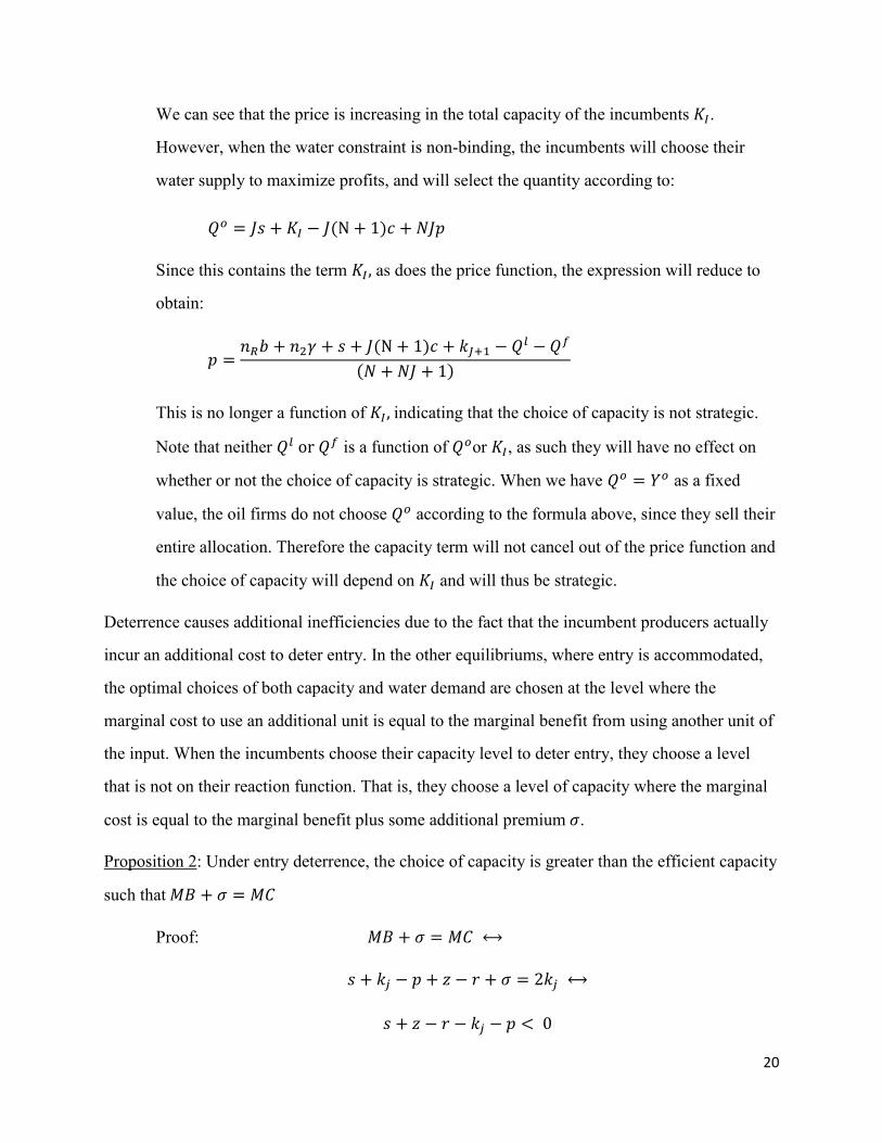
We can see that the price is increasing in the total capacity of the incumbents 𝐾𝐼.
However, when the water constraint is non-binding, the incumbents will choose their
water supply to maximize profits, and will select the quantity according to:
𝑄𝑜 = 𝐽𝑠 + 𝐾𝐼 − 𝐽(N + 1)𝑐 + 𝑁𝐽𝑝
Since this contains the term 𝐾𝐼 , as does the price function, the expression will reduce to
obtain:
𝑝 =𝑛𝑅𝑏 + 𝑛2𝛾 + 𝑠 + 𝐽(N + 1)𝑐 + 𝑘𝐽+1 − 𝑄𝑙 − 𝑄𝑓
(𝑁 + 𝑁𝐽 + 1)
This is no longer a function of 𝐾𝐼 , indicating that the choice of capacity is not strategic.
Note that neither 𝑄𝑙 or 𝑄𝑓 is a function of 𝑄𝑜or 𝐾𝐼, as such they will have no effect on
whether or not the choice of capacity is strategic. When we have 𝑄𝑜 = 𝑌𝑜 as a fixed
value, the oil firms do not choose 𝑄𝑜 according to the formula above, since they sell their
entire allocation. Therefore the capacity term will not cancel out of the price function and
the choice of capacity will depend on 𝐾𝐼 and will thus be strategic.
Deterrence causes additional inefficiencies due to the fact that the incumbent producers actually
incur an additional cost to deter entry. In the other equilibriums, where entry is accommodated,
the optimal choices of both capacity and water demand are chosen at the level where the
marginal cost to use an additional unit is equal to the marginal benefit from using another unit of
the input. When the incumbents choose their capacity level to deter entry, they choose a level
that is not on their reaction function. That is, they choose a level of capacity where the marginal
cost is equal to the marginal benefit plus some additional premium 𝜎.
Proposition 2: Under entry deterrence, the choice of capacity is greater than the efficient capacity
such that 𝑀𝐵 + 𝜎 = 𝑀𝐶
Proof: 𝑀𝐵 + 𝜎 = 𝑀𝐶 ⟷
𝑠 + 𝑘𝑗 − 𝑝 + 𝑧 − 𝑟 + 𝜎 = 2𝑘𝑗 ⟷
𝑠 + 𝑧 − 𝑟 − 𝑘𝑗 − 𝑝 < 0
Page 24
21
𝑠 + 𝑧 − 𝑟 − 𝑌𝑜 − 2(N + 1)(s − c) −(2𝑁 + 𝐽 + 2)(𝑧 − 𝑟)
2
+(2𝑁 + 𝐽 + 2)((𝑧 − 𝑟)2 + 4𝛽)
12(4𝑁2 + 4𝑁𝐽 + 16𝑁 + 𝐽2 + 8𝐽 + 14)
2(2𝑁 + 𝐽 + 2)2
− 𝑠 −𝑧 − 𝑟
2+
((𝑧 − 𝑟)2 + 4𝛽)12(4𝑁2 + 4𝑁𝐽 + 16𝑁 + 𝐽2 + 8𝐽 + 14)
2(2𝑁 + 𝐽 + 2)2
< 0
[4𝐹 − (𝑧 − 𝑟)2
(4𝑁2 + 4𝑁𝐽 + 16𝑁 + 𝐽2 + 8𝐽 + 14)]
1/2
<2(2𝑁 + 𝐽 + 2)[𝑌𝑜 + 2(N + 1)(s − c)]
(2𝑁 + 𝐽 + 3)(4𝑁2 + 4𝑁𝐽 + 16𝑁 + 𝐽2 + 8𝐽 + 14)
+(2𝑁 + 𝐽 + 2)(2𝑁 + 𝐽 + 1)(𝑧 − 𝑟)
(2𝑁 + 𝐽 + 3)(4𝑁2 + 4𝑁𝐽 + 16𝑁 + 𝐽2 + 8𝐽 + 14)
4𝐹
(𝑧 − 𝑟)2− 1
<(4𝑁2 + 4𝑁𝐽 + 16𝑁 + 𝐽2 + 8𝐽 + 14)
(𝑧 − 𝑟)2(
2(2𝑁 + 𝐽 + 2)[𝑌𝑜 + 2(N + 1)(s − c)]
(2𝑁 + 𝐽 + 3)(4𝑁2 + 4𝑁𝐽 + 16𝑁 + 𝐽2 + 8𝐽 + 14)
+(2𝑁 + 𝐽 + 2)(2𝑁 + 𝐽 + 1)(𝑧 − 𝑟)
(2𝑁 + 𝐽 + 3)(4𝑁2 + 4𝑁𝐽 + 16𝑁 + 𝐽2 + 8𝐽 + 14))
2
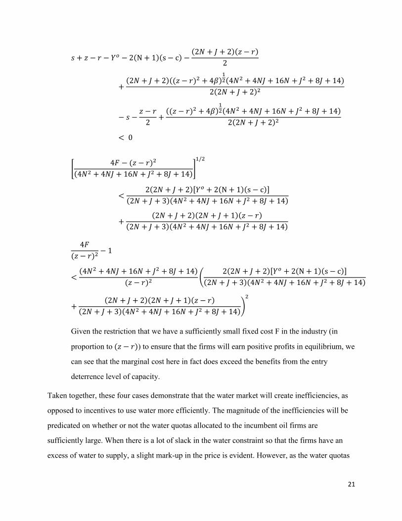
Given the restriction that we have a sufficiently small fixed cost F in the industry (in
proportion to (𝑧 − 𝑟)) to ensure that the firms will earn positive profits in equilibrium, we
can see that the marginal cost here in fact does exceed the benefits from the entry
deterrence level of capacity.
Taken together, these four cases demonstrate that the water market will create inefficiencies, as
opposed to incentives to use water more efficiently. The magnitude of the inefficiencies will be
predicated on whether or not the water quotas allocated to the incumbent oil firms are
sufficiently large. When there is a lot of slack in the water constraint so that the firms have an
excess of water to supply, a slight mark-up in the price is evident. However, as the water quotas
Page 25
22
become very restrictive as compared to the current water utilization of the industry, we see an
increasing incentive for a strategic choice of capacity in order to deter entry and lessen
competition for scarce inputs. Although this case is not of concern given the current water supply
and utilization for the industry, it becomes increasingly likely in the future due to the potential
for supply shocks and entry into the industry. The emphasis here is that the water quotas are an
important factor in determining the outcome and should water scarcity become an issue in the
region, there will likely be more discussion around alternative water policies such as a water
market to incent conservation. We have shown that, given the current industry structure, creation
of a water market under conditions of scarcity will likely have the opposite effect; firms will
choose a higher capacity than they would in the absence of a market, thereby using a greater
amount of water than would be considered efficient.
V. Conclusion
This thesis has shown that the industry outcome will be highly dependent on the initial water
quotas and on the amount of slackness between the available water and the amount of water
quantity the oil producers would like to supply in the market. Similar to the previous literature on
entry deterrence we show that an increase in investment in capacity by the incumbent producers
will result in the potential for deterrence of an entrant. However, the likelihood of deterrence
relies heavily on the ability of the incumbents to strategically manipulate the water price via their
capacity choice; this will be dependent on the existence of binding water quotas for the industry.
We have shown the unique result that the producers can manipulate the upstream market price
for water via their capacity choice to deter entry downstream.
Thus a change from the current water allocation policy to the creation of a water market will
likely not have any beneficial effects on water usage in the oil sands region. Since entry to the oil
market is likely, the market will include an inefficient mark-up on the price even when water
quotas are slack. This creates an inefficient outcome as the incumbent oil producers can increase
their profits at the expense of the entrant, who is faced with a higher water price. On the other
hand, if there is a shock which reduces the available water supply, or if there is a lot of entry into
Page 26
23
the industry, it is probable that the water quotas will become binding. We have seen that the
industry is characterized by high fixed costs so it is likely that entry deterrence will be the result,
should the industry’s water quota’s become binding. It is important to note that the water quotas
may become binding in the future due to events exogenous to the water market itself. Changes to
the scale of the mining operations, water demands for reclamation of tailings ponds, emergence
of new industries and the effects of climate change will all impact future water availability. This
suggests the potential for the oil industry to become less and less competitive under a vertically
integrated structure, an outcome which is not beneficial to the other water market participants or
to society as a whole, since deterrence will result in more water usage for oil production, above
the point water would be used in an efficient equilibrium.
Page 27
24
Bibliography
Adamowicz, W., Percy, D., & Weber, M. (2010). Alberta's Water Resource Allocation and
Management System. Alberta Innovates Energy and Environment Solutions.
Alberta Energy Regulator. (2012). Directive 081: Water Disposal Limits and Reporting
Requirements for Thermal In Situ Oil Sands Schemes.
Alberta Environment and Sustanable Resource Development. (2014). Oil sands Information
Portal.
Alberta Environment. (2010). Sectoral Water Allocations in Alberta. Alberta Environment, 2011.
Canadian Association of Petroleum Producers. (2014). Crude Oil Forecast, Markets &
Transportation. Industry publication, 2.
de Fontenay, C., & Gans, J. (2005). Vertical Integration in the Presence of Upstream
Competition. The RAND Journal of Economics, Vol. 36, No. 3 (Autumn, 2005), pp. 544-
572.
Dixit, A. (1979). A model of duopoly suggesting a theory of entry barriers. The Bell Journal of
Economics, Vol. 10, No. 1, Spring, 1979 .
Environment Canada, Water Office (Accessed 2014). Historical Hydrometric Data, Athabasca
River Below McMurray. Website: https://wateroffice.ec.gc.ca/
Gilbert, R., & Vives, X. (1986). Entry Deterrence and the Free Rider Problem. The Review of
Economic Studies, Vol. 53, No. 1 (Jan., 1986), pp. 71-83.
Griffiths, M., Taylor, A., & Woynillowicz, D. (2006). Troubled Waters, Troubling Trends.
Pembina Institute.
Pembina Institute (Accessed 2014). Oilsands Water Impacts. Website: http://www.pembina.org/.
Jasechko, S., Gibson, J., Birks, J., & Yi, Y. (2012). Quantifying saline groundwater seepage to
surface waters in the Athabasca oil sands region. Applied Geochemistry, 2068–2076.
Kuhn, K.-U., & Vives, X. (1999). Excess Entry, Vertical Integration, and Welfare. The RAND
Journal of Economics, Vol. 30, No. 4 (Winter, 1999), pp. 575-603.
Lewis, J. (2014). Imperial Oil still working out kinks at $12.9-billion Kearl oil sands mine.
Financial Post.
Normann, H. (2011). Vertical Mergers, Foreclosure and Raising Rivals' Costs - Experimental
Evidence. The Journal of Industrial Economics , Vol 59, issue 3, p506-p527.
Patterson, D. (2013). Town secures another water license. Okotoks Western Wheel Newspaper.
Page 28
25
Percy, D. (2005). Responding to Water Scarcity in Western Canada. Texas Law Review, Vol: 83,
p2091.
Salinger, M. (1988). Vertical Mergers and Market Foreclosure. The Quarterly Journal of
Economics, 103 (2): 345-356.
Schindler, D., & Donahue, W. (2006). An impending water crisis in Canada’s western Prarie
Provinces. National Academy of Sciences of the US.
Song, J.-d., & Kim, J.-C. (2001). Strategic Reaction of Vertically Integrated Firms to
Downstream Entry: Deterrence or Accommodation. Journal of Regulatory Economics,
183-199.
Spence, M. (1977). Entry, capacity, investment and oligopolistic pricing. The Bell Journal of
Economics, Vol. 8, No. 2, Autumn, 1977.
Tomkins, C., & Weber, T. (2010). Option contracting in the California water market. Journal of
Regulatory Economics, April 2010, v. 37, iss. 2, pp. 107-41.
Walkem, A. (2007). Eau Canada, The Future of Canada's Water. Vancouver: UBC Press.
Young, M., & McColl, J. (2003). Robust Reform: The Case for a New Water Entitlement System
for Australia. Australian Economic Review, June, v. 36, iss. 2, pp. 225-34.
Page 29
26
VI. Appendix
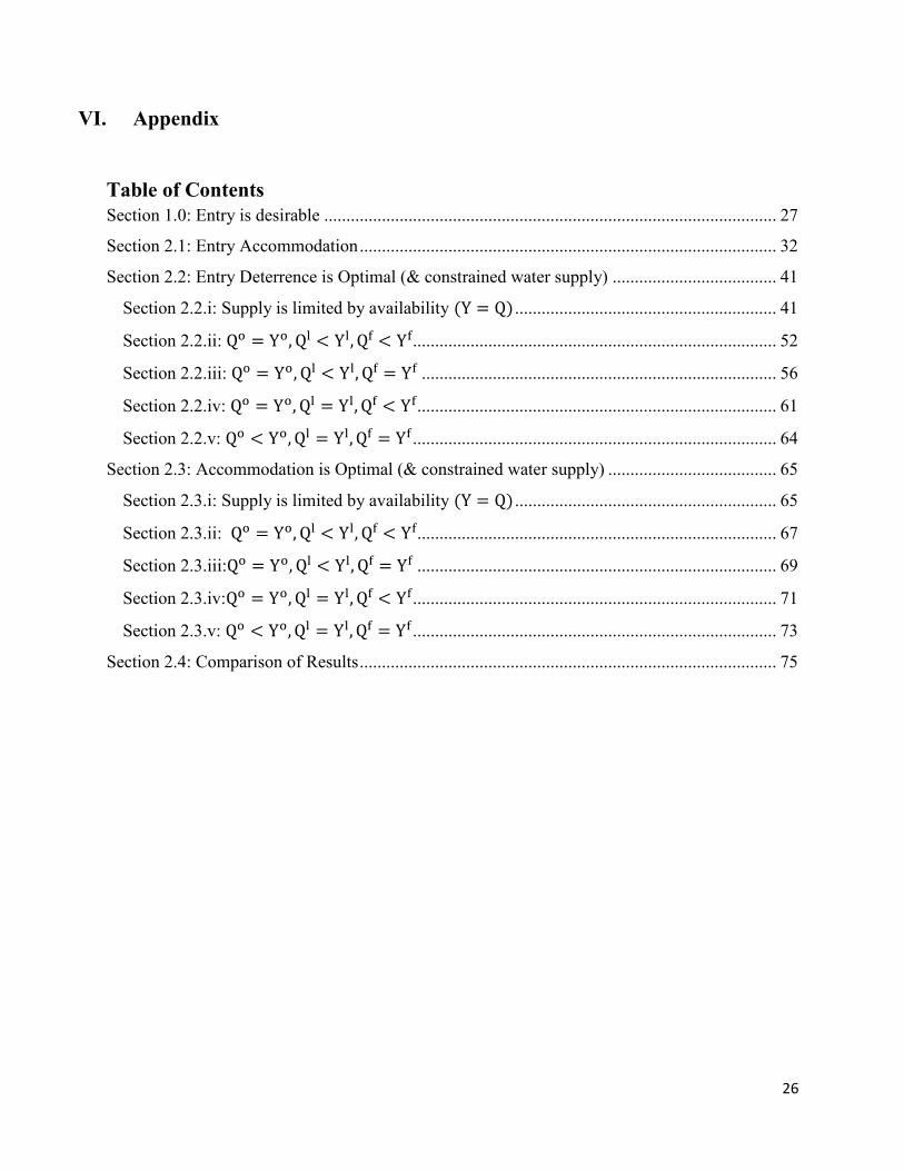
Table of Contents
Section 1.0: Entry is desirable ...................................................................................................... 27
Section 2.1: Entry Accommodation .............................................................................................. 32
Section 2.2: Entry Deterrence is Optimal (& constrained water supply) ..................................... 41
Section 2.2.i: Supply is limited by availability (Y = Q) ........................................................... 41
Section 2.2.ii: Qo = Yo, Ql < Yl, Qf < Yf .................................................................................. 52
Section 2.2.iii: Qo = Yo, Ql < Yl, Qf = Yf ................................................................................ 56
Section 2.2.iv: Qo = Yo, Ql = Yl, Qf < Yf ................................................................................. 61
Section 2.2.v: Qo < Yo, Ql = Yl, Qf = Yf .................................................................................. 64
Section 2.3: Accommodation is Optimal (& constrained water supply) ...................................... 65
Section 2.3.i: Supply is limited by availability (Y = Q) ........................................................... 65
Section 2.3.ii: Qo = Yo, Ql < Yl, Qf < Yf ................................................................................. 67
Section 2.3.iii:Qo = Yo, Ql < Yl, Qf = Yf ................................................................................. 69
Section 2.3.iv:Qo = Yo, Ql = Yl, Qf < Yf .................................................................................. 71
Section 2.3.v: Qo < Yo, Ql = Yl, Qf = Yf .................................................................................. 73
Section 2.4: Comparison of Results .............................................................................................. 75
Page 30
27
Section 1.0: Entry is desirable
Water Demand:
i. Local Community: n1 consumers
ii. First Nations: n2 consumers
iii. Oil Producers: J producers
Final Water Consumers: n1 + n2 = nR
Water Suppliers:
Local Community is endowed with Yl units of water
First Nations are endowed with Yf units of water
Oil Producers are endowed with Yo units of water
Let 𝑌 = Y𝑙 + Y𝑓 + Y𝑜 be fixed.
In this scenario, the quantities sold will be less than the endowments Yi
Stage 3: Find water demand
Utility of a representative final consumer i:
𝑥𝑖 + 𝑎𝑖 (𝑏 −𝑎𝑖
2)
Budget Constraints:
𝑤𝑖 = 𝑥𝑖 + 𝑝𝑎𝑎𝑖 ∀ 𝑖 = 1, … , 𝑛𝑅
Where:
𝑥𝑖 = Utility derived from the basket of consumer goods
𝑎𝑖 = Water demand (final)
𝑎𝑜 = Water usage (intermediate, oil producers)
𝑎𝑓 = Water usage (intermediate, First Nation)
𝑝 = Price of water
𝑤𝑖 = Income or wealth
Utility Maximization for final water consumer i:
max{𝑎𝑖}( 𝑥𝑖 + 𝑎𝑖(𝑏 − 𝑎𝑖2
) − 𝑝𝑎𝑖)
Then 0 = −𝑝 + 𝑏 − 𝑎𝑖
⟹ 𝑎𝑖(𝑝; 𝑏) = 𝑏 − 𝑝
Income Maximization for intermediate First Nations production
max{𝑎𝑓}( 𝑎𝑓 (𝛾 − 𝑎𝑓
2) − 𝑝𝑎𝑓)
Then 0 = −𝑝 + 𝛾 − 𝑎𝑓
⟹ 𝑎𝑓(𝑝; 𝛾) = 𝛾 − 𝑝
Page 31
28
Profit maximization for oil producers (in the oil market):
Π𝑠𝑒 = 𝑒(𝑎𝑜; 𝑘𝑗) − 𝑝𝑎𝑜 − 𝑘𝑗𝑟 = 𝑎𝑜 (𝑠 −
𝑎𝑜
2) + 𝑘𝑗(𝑧 − 𝑘𝑗) + 𝑎𝑜𝑘𝑗 − 𝑝𝑎𝑜 − 𝑘𝑗𝑟 − 𝐹
Where
𝑘𝑗 = Capacity or capital cost for producer j
z and s are constants
r= price of capital
F= fixed cost
max{𝑎𝑜}
(Π𝑠𝑒) = max
{𝑎𝑜}[𝑎𝑜 (𝑠 −
𝑎𝑜
2) + 𝑘𝑗(𝑧 − 𝑘𝑗) + 𝑎𝑜𝑘𝑗 − 𝑝𝑎𝑜 − 𝑘𝑗𝑟 − 𝐹]
Then 0 = 𝑠 + 𝑘𝑗 − 𝑎𝑜 − 𝑝
⟹ 𝑎𝑜(𝑝; 𝑘𝑗) = 𝑠 + 𝑘𝑗 − 𝑝
Let:
𝐾𝐼 = ∑ 𝑘𝑗
𝐽
1
Supply of Water
For final consumers: 𝑛𝑅 ∙ 𝑎𝑖(𝑝; 𝑏)
For intermediate First Nation: 𝑛2 ∙ 𝑎𝑓(𝑝; 𝛾)
For incumbent oil producers: 𝐽 ∙ 𝑎𝑜(𝑝; 𝑘𝑗)
Market clearing condition:
𝑄 = 𝑛𝑅 ∙ 𝑎𝑖(𝑝; 𝑏) + 𝑛2 ∙ 𝑎𝑓(𝑝; 𝛾) + 𝐽 ∙ 𝑎𝑜(𝑝; 𝑘𝑗)
𝑄 = 𝑛𝑅(𝑏 − 𝑝) + 𝑛2(𝛾 − 𝑝) + 𝐾𝐼 + 𝐽(𝑠 − 𝑝)
𝑄 = 𝑏𝑛𝑅 + 𝑛2𝛾 + 𝐽𝑠 + 𝐾𝐼 − 𝑝(𝑛𝑅 + 𝑛2 + 𝐽)
Let 𝑁 = 𝑛𝑅 + 𝑛2 + 𝐽
Producer demand function
𝑝(𝑄, 𝐾𝐼) =𝑛𝑅𝑏 + 𝑛2𝛾 + 𝐽𝑠 + 𝐾𝐼 − 𝑄
𝑁
Where 𝑑𝑝
𝑑𝑄= −
1
𝑁
Stage 2: All groups choose water supply simultaneously
a. Oil producers will choose 𝑞𝑗𝑜 ∈ (0, 𝑦𝑜) to maximize Π𝑗 , where
Page 32
29
𝑄𝑜 = ∑ 𝑞𝑗𝑜
𝐽
𝑠=1
𝑎𝑛𝑑 𝑌𝑜 = ∑ 𝑦𝑜
𝐽
1
max{𝑞𝑗
𝑜}((𝑝 − 𝑐)𝑞𝑗
𝑜 + 𝑎𝑜 (𝑠 −𝑎𝑜
2) + 𝑘𝑗(𝑧 − 𝑘𝑗) + 𝑎𝑜𝑘𝑗 − 𝑝𝑎𝑜 − 𝑘𝑗𝑟 − 𝐹)
max{𝑞𝑗
𝑜}((𝑝 − 𝑐)𝑞𝑗
𝑜 + (1
2)(𝑠 + 𝑘𝑗 − 𝑝)
2+ 𝑘𝑗(𝑧 − 𝑘𝑗) − 𝑘𝑗𝑟 − 𝐹)
⟹ (𝑑𝑝
𝑑𝑄𝑞𝑗
𝑜 + (𝑝 − 𝑐) − (𝑠 + 𝑘𝑗 − 𝑝)𝑑𝑝
𝑑𝑄) = 0
𝑞𝑗𝑜 = 𝑠 + 𝑘𝑗 − 𝑁𝑐 + (𝑁 − 1)𝑝
Since 𝑄𝑜 = 𝐽𝑞𝑗𝑜
𝑄𝑜 = 𝐽𝑞𝑗𝑜 = 𝐽𝑠 + 𝐾𝐼 − 𝐽N𝑐 + (𝑁 − 1)𝐽𝑝
b. Local Community
The local community has indirect utility function:
𝑣𝑖(∙) = 𝑥𝑖 +(𝑏 − 𝑝)2
2
Where
𝑥𝑖 =(𝑝 − 𝑐)𝑄𝑙 + 𝐽𝛱𝑗
𝑛1
The local government will choose 𝑄𝑙 ∈ (0, 𝑌𝑙) to maximize:
Π𝑙 = (𝑝 − 𝑐)𝑄𝑙 + 𝐽Π𝑗 +𝑛1
2(𝑏 − 𝑝)2
First Order conditions:
𝑑𝑝
𝑑𝑄𝑄𝑙 + (p − c) − 𝑛1(𝑏 − 𝑝)
𝑑𝑝
𝑑𝑄= 0
−𝑄𝑙
𝑁+ p − c +
𝑛1
𝑁(𝑏 − 𝑝) = 0
𝑄𝑙 = 𝑛1𝑏 − 𝑁𝑐 + 𝑝(𝑁 − 𝑛1)
c. First Nation
First Nations will maximize profits:
Π𝑓 = Π𝑠𝑓𝑎
+ Π𝑠𝑔
𝛱𝑓 = (𝑝 − 𝑐)𝑄𝑓 + 12⁄ (𝛾 − 𝑝)2
Need to add the consumer surplus to the First Nations producer surplus.
Page 33
30
A resident i in the First Nations will maximize their utility as follows:
max{𝑎𝑖}( 𝑤𝑖 − 𝑝𝑎𝑖 + 𝑎𝑖(𝑏 − 𝑎𝑖2
)) which yields: 𝑎𝑖(𝑝; 𝑏) = 𝑏 − 𝑝
Substitute the demand functions into the objective function to derive the indirect utility
function for a representative resident ί.
𝑣𝑖(𝑤𝑖, 𝑝, 𝑏) = 𝑤𝑖 − 𝑝(𝑏 − 𝑝) + (𝑏 − 𝑝) (𝑏 −(𝑏−𝑝)
2)
𝑣𝑖(∙) = 𝑤𝑖 + (𝑏 − 𝑝) (𝑏 − 𝑝 −(𝑏−𝑝)
2)
𝑣𝑖(∙) = 𝑤𝑖 +(𝑏 − 𝑝)2
2
Where 𝑤𝑖 = Π𝑓
𝑛2⁄
The First Nations government chooses 𝑄𝑓 ∈ (0, 𝑌𝑓) to maximize:
𝛱𝑓 = (𝑝 − 𝑐)𝑄𝑓 +𝑛2
2(𝛾 − 𝑝)2 +
𝑛2
2(𝑏 − 𝑝)2
Assuming an interior solution, the first order condition is: 𝑑𝑝
𝑑𝑄𝑄𝑓 + (p − c) − 𝑛2(𝛾 − 𝑝)
𝑑𝑝
𝑑𝑄− 𝑛2(𝑏 − 𝑝)
𝑑𝑝
𝑑𝑄= 0
−𝑄𝑓
𝑁+ (p − c) +
𝑛2
𝑁(𝛾 − 𝑝) +
𝑛2
𝑁(𝑏 − 𝑝) = 0
𝑄𝑓 = 𝑛2(𝛾 + 𝑏) − Nc + p(𝑁 − 2𝑛2)
So, we have:
𝑄 = 𝑄𝑜 + 𝑄𝑓 + 𝑄𝑙 where
𝑄𝑜 = 𝐽𝑠 + 𝐾𝐼 − 𝐽𝑁𝑐 + (𝑁 − 1)𝐽𝑝
𝑄𝑓 = 𝑛2(𝛾 + 𝑏) − Nc + p(𝑁 − 2𝑛2)
𝑄𝑙 = 𝑛1𝑏 − 𝑁𝑐 + 𝑝(𝑁 − 𝑛1)
Find the quantities of water:
𝑄 = 𝐽𝑠 + 𝐾𝐼 − 𝐽𝑁𝑐 + (𝑁 − 1)𝐽𝑝 + 𝑛2(𝛾 + 𝑏) − Nc + p(𝑁 − 2𝑛2) + 𝑛1𝑏 − 𝑁𝑐 + 𝑝(𝑁− 𝑛1)
𝑄 = 𝑛𝑅𝑏 + 𝑛2𝛾 + 𝐽𝑠 + 𝐾𝐼 − 𝑁𝑐(𝐽 + 2) + p(2𝑁 + 𝑁𝐽 − 𝐽 − 𝑛𝑅 − 𝑛2)
𝑄 = 𝑛𝑅𝑏 + 𝑛2𝛾 + 𝐽𝑠 + 𝐾𝐼 − 𝑁𝑐(𝐽 + 2) + pN(𝐽 + 1)
𝑄 = 𝑛𝑅𝑏 + 𝑛2𝛾 + 𝐽𝑠 + 𝐾𝐼 − 𝑁𝑐(𝐽 + 2) + N(𝐽 + 1) [𝑛𝑅𝑏 + 𝑛2𝛾 + 𝐽𝑠 + 𝐾𝐼 − 𝑄
𝑁]
𝑄(2𝑁 + 𝑁𝐽) = (𝑛𝑅𝑏 + 𝑛2𝛾 + 𝐽𝑠 + 𝐾𝐼)(2𝑁 + 𝑁𝐽) − 𝑁2𝑐(𝐽 + 2)
𝑄 = 𝑛𝑅𝑏 + 𝑛2𝛾 + 𝐽𝑠 + 𝐾𝐼 − 𝑐 (𝑁2(𝐽 + 2)
𝑁(𝐽 + 2))
Page 34
31
𝑄 = 𝑛𝑅𝑏 + 𝑛2𝛾 + 𝐽𝑠 + 𝐾𝐼 − 𝑁𝑐
𝑝 =𝑛𝑅𝑏 + 𝑛2𝛾 + 𝐽𝑠 + 𝐾𝐼 − [𝑛𝑅𝑏 + 𝑛2𝛾 + 𝐽𝑠 + 𝐾𝐼 − 𝑁𝑐]
𝑁
𝑝∗ = 𝑐
Stage 1: Oil producers choose capacity kj
max{𝑘𝑗}
(𝑞𝑗𝑜(𝑝 − 𝑐) + (
1
2) (𝑠 + 𝑘𝑗 − 𝑝)
2+ 𝑘𝑗(𝑧 − 𝑘𝑗 − 𝑟) − 𝐹)
𝑞𝑗𝑜 𝑑𝑝
𝑑𝐾+ 𝑠 + 𝑘𝑗 − 𝑠
𝑑𝑝
𝑑𝐾− 𝑘𝑗
𝑑𝑝
𝑑𝐾− 𝑝 + 𝑝
𝑑𝑝
𝑑𝐾+ 𝑧 − 2𝑘𝑗 − 𝑟 = 0
1
𝑁(𝑞𝑗
𝑜 − 𝑠 − 𝑘𝑗 + 𝑝) + 𝑠 − 𝑘𝑗 − 𝑝 + 𝑧 − 𝑟 = 0
(𝑞𝑗𝑜 − 𝑠 − 𝑘𝑗 + 𝑝) + 𝑁(𝑠 − 𝑘𝑗 − 𝑝 + 𝑧 − 𝑟) = 0
𝑘𝑗 =𝑁(𝑧 − 𝑟) + (𝑁 − 1)𝑠 − (𝑁 − 1)𝑝 + 𝑞𝑗
𝑜
𝑁 + 1
𝑘𝑗 =𝑁(𝑧 − 𝑟) + (𝑁 − 1)𝑠 − (𝑁 − 1)𝑝 + 𝑠 + 𝑘𝑗 − 𝑁𝑐 + (𝑁 − 1)𝑝
𝑁 + 1
𝑁𝑘𝑗 = 𝑁(𝑧 − 𝑟) + 𝑁𝑠 − 𝑁𝑐
𝑘𝑗∗ = (𝑧 − 𝑟) + 𝑠 − 𝑐
Results:
𝐾𝐼∗ = 𝐽(𝑧 − 𝑟) + 𝐽𝑠 − 𝐽𝑐
𝑄∗ = 𝑛𝑅𝑏 + 𝑛2𝛾 + 2𝐽𝑠 + 𝐽(𝑧 − 𝑟) − (𝐽 + 𝑁)𝑐
𝑝∗ = 𝑐
𝑄𝑜∗ = 2𝐽𝑠 + 𝐽(𝑧 − 𝑟) − 2𝐽𝑐
𝑄𝑓∗= 𝑛2(𝛾 + 𝑏) − 2𝑛2c
𝑄𝑙∗= 𝑛1𝑏 − 𝑛1𝑐
Π𝑓∗=
𝑛2
2[(𝛾 − 𝑐)2 + ((𝑏 − 𝑐)2]
Π𝑙∗= 𝐽Π𝑗
∗ +𝑛1
2(𝑏 − 𝑐)2
Π𝑗∗ = [2𝑠 + (𝑧 − 𝑟) − 2𝑐](𝑝∗ − 𝑐) + (
1
2) (𝑠 + 𝑘𝑗 − 𝑝)
2+ 𝑘𝑗(𝑧 − 𝑘𝑗 − 𝑟) − 𝐹
Page 35
32
Π𝑗∗ = (
1
2) (2𝑠 + (𝑧 − 𝑟) − 2𝑐)2 − ((𝑧 − 𝑟) + 𝑠 − 𝑐)
2+ (𝑧 − 𝑟)((𝑧 − 𝑟) + 𝑠 − 𝑐) − 𝐹
Π𝑗∗ = (
1
2) (𝑠 − 𝑐)2 + (
1
2) (𝑠 − 𝑐 + (𝑧 − 𝑟))
2− 𝐹
Π𝑗∗ = (𝑠 − 𝑐)2 + (𝑠 − 𝑐)(𝑧 − 𝑟) + (
1
2) (𝑧 − 𝑟)2 − 𝐹
Section 2.1: Entry Accommodation
Water Demand:
i. Local Community: n1 consumers
ii. First Nations: n2 consumers
iii. Oil Producers: J producers
iv. New Entrant (oil market): J+1th
producer
Water Suppliers:
Local Community is endowed with Yl units of water
First Nations are endowed with Yf units of water
Oil Producers are endowed with Yo units of water
Let 𝑌 = Y𝑙 + Y𝑓 + Y𝑜 be fixed.
Stage 4: Find water demands
Supply of Water (derived in section 1)
For final consumers: 𝑛𝑅 ∙ 𝑎𝑖(𝑝; 𝑏)
For intermediate First Nation: 𝑛2 ∙ 𝑎𝑓(𝑝; 𝛾)
For incumbent oil producers: 𝐽 ∙ 𝑎𝑜(𝑝; 𝑘𝑗)
For entrant: 𝑎𝑜(𝑝; 𝑘𝐽+1)
Market clearing condition:
𝑄 = 𝑛𝑅 ∙ 𝑎𝑖(𝑝; 𝑏) + 𝑛2 ∙ 𝑎𝑓(𝑝; 𝛾) + 𝐽 ∙ 𝑎𝑜(𝑝; 𝑘𝑗) + 𝑎𝑜(𝑝; 𝑘𝐽+1)
𝑄 = 𝑛𝑅(𝑏 − 𝑝) + 𝑛2(𝛾 − 𝑝) + 𝐾𝐼 + 𝐽(𝑠 − 𝑝) + 𝑠 + 𝑘𝐽+1 − 𝑝
𝑄 = 𝑏𝑛𝑅 + 𝑛2𝛾 + (𝐽 + 1)𝑠 + 𝐾𝐼 + 𝑘𝐽+1 − 𝑝(𝑛𝑅 + 𝑛2 + 𝐽 + 1)
Let 𝑁 = 𝑛𝑅 + 𝑛2 + 𝐽
Producer demand function
𝑃(𝑄, 𝐾𝐼 , 𝑘𝐽+1) =𝑛𝑅𝑏 + 𝑛2𝛾 + (𝐽 + 1)𝑠 + 𝐾𝐼 + 𝑘𝐽+1 − 𝑄
𝑁 + 1
Page 36
33
Where 𝑑𝑝
𝑑𝑄= −
1
𝑁+1
Stage 3: All groups choose water supply simultaneously
a. Oil producers:
max{𝑞𝑗
𝑜}((𝑝 − 𝑐)𝑞𝑗
𝑜 + (1
2)(𝑠 + 𝑘𝑗 − 𝑝)
2+ 𝑘𝑗(𝑧 − 𝑘𝑗) − 𝑘𝑗𝑟 − 𝐹)
⟹ (𝑑𝑝
𝑑𝑄𝑞𝑗
𝑜 + (𝑝 − 𝑐) − (𝑠 + 𝑘𝑗 − 𝑝)𝑑𝑝
𝑑𝑄) = 0
𝑞𝑗𝑜 = 𝑠 + 𝑘𝑗 − (𝑁 + 1)𝑐 + 𝑁𝑝
Since 𝑄𝑜 = 𝐽𝑞𝑗𝑜
𝑄𝑜 = 𝐽𝑞𝑗𝑜 = 𝐽𝑠 + 𝐾𝐼 − 𝐽(𝑁 + 1)𝑐 + 𝑁𝐽𝑝
b. Local Community
The local government will choose 𝑄𝑙 ∈ (0, 𝑌1) to maximize:
Π𝑙 = (p − 𝑐)𝑄𝑙 + 𝐽Π𝑓 +𝑛1
2(𝑏 − 𝑝)2
First Order conditions:
𝑑𝑝
𝑑𝑄𝑄𝑙 + (p − c) − 𝑛1(𝑏 − 𝑝)
𝑑𝑝
𝑑𝑄= 0
−𝑄𝑙
𝑁 + 1+ p − c +
𝑛1
𝑁 + 1(𝑏 − 𝑝) = 0
𝑄𝑙 = 𝑛1𝑏 − (𝑁 + 1)𝑐 + 𝑝(𝑁 + 1 − 𝑛1)
c. First Nation
The First Nations government chooses 𝑄𝑓 ∈ (0, 𝑌2) to maximize:
Π𝑓 = (p − c)𝑄𝑓 +𝑛2
2(𝛾 − 𝑝)2 +
𝑛2
2(𝑏 − 𝑝)2
Assuming an interior solution, the first order condition is: 𝑑𝑝
𝑑𝑄𝑄𝑓 + (p − c) − 𝑛2(𝛾 − 𝑝)
𝑑𝑝
𝑑𝑄− 𝑛2(𝑏 − 𝑝)
𝑑𝑝
𝑑𝑄= 0
−𝑄𝑓
𝑁 + 1+ (p − c) +
𝑛2
𝑁 + 1(𝛾 − 𝑝) +
𝑛2
𝑁 + 1(𝑏 − 𝑝) = 0
𝑄𝑓 = p(𝑁 + 1 − 𝑛2 − 𝑛2) − (N + 1)c + 𝑛2𝛾 + 𝑛2𝑏
𝑄𝑓 = 𝑛2(𝛾 + 𝑏) − (N + 1)c + p(𝑁 + 1 − 2𝑛2)
Page 37
34
So, we have:
𝑄 = 𝑄𝑜 + 𝑄𝑓 + 𝑄𝑙 where
𝑄𝑜 = 𝐽𝑠 + 𝐾𝐼 − 𝐽(𝑁 + 1)𝑐 + 𝑁𝐽𝑝
𝑄𝑓 = 𝑛2(𝛾 + 𝑏) − (N + 1)c + p(𝑁 + 1 − 2𝑛2)
𝑄𝑙 = 𝑛1𝑏 − (𝑁 + 1)𝑐 + 𝑝(𝑁 + 1 − 𝑛1)
Find the quantities of water:
𝑄 = 𝐽𝑠 + 𝐾𝐼 − 𝐽(𝑁 + 1)𝑐 + 𝑁𝐽𝑝 + 𝑛2(𝛾 + 𝑏) − (N + 1)c + p(𝑁 + 1 − 2𝑛2) + 𝑛2(𝛾 + 𝑏)− (N + 1)c + p(𝑁 + 1 − 2𝑛2)
𝑄 = 𝐽𝑠 + 𝑛2𝛾 + 𝑛𝑅𝑏 + 𝐾𝐼 − (𝐽 + 2)(𝑁 + 1)𝑐 + p(𝐽𝑁 + 𝑁 + 𝐽 + 2)
𝑄 = 𝐽𝑠 + 𝑛2𝛾 + 𝑛𝑅𝑏 + 𝐾𝐼 − (𝐽 + 2)(𝑁 + 1)𝑐
+ (𝐽𝑁 + 𝑁 + 𝐽 + 2) [𝑛𝑅𝑏 + 𝑛2𝛾 + (𝐽 + 1)𝑠 + 𝐾𝐼 + 𝑘𝐽+1 − 𝑄
𝑁 + 1]
𝑄(𝐽𝑁 + 2𝑁 + 𝐽 + 3)= (𝑁 + 1)[𝐽𝑠 + 𝑛2𝛾 + 𝑛𝑅𝑏 + 𝐾𝐼] − (𝐽 + 2)(𝑁 + 1)2𝑐
+ (𝐽𝑁 + 𝑁 + 𝐽 + 2)[𝑛𝑅𝑏 + 𝑛2𝛾 + (𝐽 + 1)𝑠 + 𝐾𝐼 + 𝑘𝐽+1]
𝑄 = 𝐽𝑠 + 𝑛2𝛾 + 𝑛𝑅𝑏 + 𝐾𝐼 +(𝐽𝑁 + 𝑁 + 𝐽 + 2)(𝑠 + 𝑘𝐽+1) − (𝐽 + 2)(𝑁 + 1)2𝑐
𝐽𝑁 + 2𝑁 + 𝐽 + 3
Then the price becomes:
𝑝 = (1
𝑁 + 1) [𝑠 + 𝑘𝐽+1 +
(𝐽 + 2)(𝑁 + 1)2𝑐 − (𝐽𝑁 + 𝑁 + 𝐽 + 2)(𝑠 + 𝑘𝐽+1)
𝐽𝑁 + 2𝑁 + 𝐽 + 3]
𝑝 = [𝑠 + 𝑘𝐽+1 + (𝐽 + 2)(𝑁 + 1)𝑐
𝐽𝑁 + 2𝑁 + 𝐽 + 3]
Stage 2: Entrant J+1 chooses capacity 𝑘𝐽+1
max{𝑘𝐽+1}
((1
2) (𝑠 + 𝑘𝑗 − 𝑝)
2+ 𝑘𝐽+1(𝑧 − 𝑘𝐽+1 − 𝑟) − 𝐹)
𝑠 − 𝑘𝐽+1 − 𝑝 + 𝑧 − 𝑟 + (𝑝 − 𝑠 − 𝑘𝐽+1)𝑑𝑝
𝑑𝐾= 0
Page 38
35
(𝑁 + 1)(𝑠 − 𝑘𝐽+1 − 𝑝 + 𝑧 − 𝑟) + 𝑝 − 𝑠 − 𝑘𝐽+1 = 0
𝑘𝐽+1 =(𝑁 + 1)(𝑧 − 𝑟) + 𝑁𝑠 − 𝑁𝑝
𝑁 + 2
𝑘𝐽+1(𝑁 + 2) = (𝑁 + 1)(𝑧 − 𝑟) + 𝑁𝑠 − 𝑁 (𝑠 + 𝑘𝐽+1 + (𝐽 + 2)(𝑁 + 1)𝑐
𝐽𝑁 + 2𝑁 + 𝐽 + 3)
𝑘𝐽+1(𝑁 + 2)(𝐽𝑁 + 2𝑁 + 𝐽 + 3)
= (𝐽𝑁 + 2𝑁 + 𝐽 + 3)(𝑁 + 1)(𝑧 − 𝑟) + (𝐽𝑁 + 2𝑁 + 𝐽 + 3)𝑁𝑠
− 𝑁(𝑠 + 𝑘𝐽+1 + (𝐽 + 2)(𝑁 + 1)𝑐)
𝑘𝐽+1[(𝑁 + 2)(𝐽𝑁 + 2𝑁 + 𝐽 + 3) + 𝑁]
= (𝐽𝑁 + 2𝑁 + 𝐽 + 3)(𝑁 + 1)(𝑧 − 𝑟) + (𝐽𝑁 + 2𝑁 + 𝐽 + 2)𝑁𝑠
− 𝑁(𝐽 + 2)(𝑁 + 1)𝑐
𝑘𝐽+1∗∗ =
(𝐽𝑁 + 2𝑁 + 𝐽 + 3)(𝑁 + 1)(𝑧 − 𝑟) + (𝐽𝑁 + 2𝑁 + 𝐽 + 2)𝑁(𝑠 − 𝑐)
(𝑁 + 2)(𝐽𝑁 + 2𝑁 + 𝐽 + 3) + 𝑁
Interpretation: since 𝑃(𝑄, 𝐾𝐼 , 𝑘𝐽+1) becomes a function of 𝑘𝐽+1only once we solve for Q, this
means that the incumbent’s choice of capacity does not depend on the entrant and they have no
incentive to deter entry under this scenario.
Stage 1: Incumbents choose kj to maximize profits
max{𝑘𝑗}
(𝑞𝑗𝑜(𝑝 − 𝑐) + (
1
2) (𝑠 + 𝑘𝑗 − 𝑝)
2+ 𝑘𝑗(𝑧 − 𝑘𝑗 − 𝑟) − 𝐹)
𝑞𝑗𝑜 𝑑𝑝
𝑑𝐾+ 𝑠 + 𝑘𝑗 − 𝑠
𝑑𝑝
𝑑𝐾− 𝑘𝑗
𝑑𝑝
𝑑𝐾− 𝑝 + 𝑝
𝑑𝑝
𝑑𝐾+ 𝑧 − 2𝑘𝑗 − 𝑟 = 0
𝑘𝑗 =(𝑁 + 1)(𝑧 − 𝑟) + 𝑁𝑠 − 𝑁𝑝 + 𝑞𝑗
𝑜
𝑁 + 2
𝐾𝐼 =𝐽(𝑁 + 1)(𝑧 − 𝑟) + 𝑁𝐽𝑠 − 𝑁𝐽𝑝 + 𝑄𝑜
𝑁 + 2
𝐾𝐼∗∗ = 𝐽(𝑧 − 𝑟) + 𝐽𝑠 − 𝐽𝑐
𝑘𝑗∗∗ = (𝑧 − 𝑟) + 𝑠 − 𝑐
Page 39
36
Results:
𝑘𝐽+1∗∗ =
(𝐽𝑁 + 2𝑁 + 𝐽 + 3)(𝑁 + 1)(𝑧 − 𝑟)
(𝑁 + 2)(𝐽𝑁 + 2𝑁 + 𝐽 + 3) + 𝑁+
𝑁(𝐽𝑁 + 2𝑁 + 𝐽 + 2)[𝑠 − 𝑐]
(𝑁 + 2)(𝐽𝑁 + 2𝑁 + 𝐽 + 3) + 𝑁
(𝐽𝑁 + 2𝑁 + 𝐽 + 3)𝑝
= 𝑠 + (𝐽 + 2)(𝑁 + 1)𝑐 +(𝐽𝑁 + 2𝑁 + 𝐽 + 3)(𝑁 + 1)(𝑧 − 𝑟)
(𝑁 + 2)(𝐽𝑁 + 2𝑁 + 𝐽 + 3) + 𝑁
+𝑁(𝐽𝑁 + 2𝑁 + 𝐽 + 2)[𝑠 − 𝑐]
(𝑁 + 2)(𝐽𝑁 + 2𝑁 + 𝐽 + 3) + 𝑁
𝑝∗∗ =𝑠 + (𝐽 + 2)(𝑁 + 1)𝑐
𝐽𝑁 + 2𝑁 + 𝐽 + 3+
(𝑁 + 1)(𝑧 − 𝑟)
(𝑁 + 2)(𝐽𝑁 + 2𝑁 + 𝐽 + 3) + 𝑁
+𝑁(𝐽𝑁 + 2𝑁 + 𝐽 + 2)[𝑠 − 𝑐]
(𝐽𝑁 + 2𝑁 + 𝐽 + 3)[(𝑁 + 2)(𝐽𝑁 + 2𝑁 + 𝐽 + 3) + 𝑁]
𝐾𝐼∗∗ = 𝐽(𝑧 − 𝑟) + 𝐽𝑠 − 𝐽𝑐
𝑘𝑗∗∗ = (𝑧 − 𝑟) + 𝑠 − 𝑐
𝑎𝑖∗∗ = (𝑏 − 𝑝∗∗)
𝑎𝑓∗∗= (𝛾 − 𝑝∗∗)
𝑎𝑜∗∗= (𝑠 + 𝑘𝑗
∗∗∗ − 𝑝∗∗)
𝑎𝑜∗∗ = 𝑠 + 𝑘𝑗∗∗∗ −
𝑠 + (𝐽 + 2)(𝑁 + 1)𝑐
𝐽𝑁 + 2𝑁 + 𝐽 + 3−
(𝑁 + 1)(𝑧 − 𝑟)
(𝑁 + 2)(𝐽𝑁 + 2𝑁 + 𝐽 + 3) + 𝑁
−𝑁(𝐽𝑁 + 2𝑁 + 𝐽 + 2)[𝑠 − 𝑐]
(𝐽𝑁 + 2𝑁 + 𝐽 + 3)[(𝑁 + 2)(𝐽𝑁 + 2𝑁 + 𝐽 + 3) + 𝑁]
𝑄∗∗ = 2𝐽𝑠 + 𝑛2𝛾 + 𝑛𝑅𝑏 + 𝐽(𝑧 − 𝑟) − 𝐽𝑐 +(𝐽𝑁 + 𝑁 + 𝐽 + 2)(𝑠 + 𝑘𝐽+1) − (𝐽 + 2)(𝑁 + 1)2𝑐
𝐽𝑁 + 2𝑁 + 𝐽 + 3
𝑞𝑗𝑜∗∗
= 2𝑠 + (𝑧 − 𝑟) − 2𝑐 + 𝑁(𝑝∗∗ − 𝑐)
𝑄𝑜∗∗ = 𝐽[2𝑠 − (𝑁 + 2)𝑐 + (𝑧 − 𝑟) + 𝑁𝑝∗∗]
𝑄𝑜∗∗ = 𝐽2𝑠 − 𝐽(𝑁 + 2)𝑐 + 𝐽(𝑧 − 𝑟) +𝑁𝐽𝑠 + 𝑁𝐽(𝐽 + 2)(𝑁 + 1)𝑐
𝐽𝑁 + 2𝑁 + 𝐽 + 3+
𝑁𝐽(𝑁 + 1)(𝑧 − 𝑟)
(𝑁 + 2)(𝐽𝑁 + 2𝑁 + 𝐽 + 3) + 𝑁
+𝑁2𝐽(𝐽𝑁 + 2𝑁 + 𝐽 + 2)[𝑠 − 𝑐]
(𝐽𝑁 + 2𝑁 + 𝐽 + 3)[(𝑁 + 2)(𝐽𝑁 + 2𝑁 + 𝐽 + 3) + 𝑁]
𝑄𝑓∗∗= 𝑛2(𝛾 + 𝑏) − (N + 1)c + 𝑝∗∗(𝑁 + 1 − 2𝑛2)
Π𝑓∗∗= (𝑝∗∗ − 𝑐)𝑄𝑓 +
𝑛2
2[(𝛾 − 𝑝∗∗)2 + (𝑏 − 𝑝∗∗)2]
Page 40
37
Π𝑓∗∗= (𝑝∗∗ − 𝑐)[𝑛2(𝛾 + 𝑏) − (N + 1)c + 𝑝∗∗(𝐽 + 1 + 𝑛1)] +
𝑛2
2[(𝛾 − 𝑝∗∗)2 + (𝑏 − 𝑝∗∗)2]
𝑄𝑙∗∗= 𝑛1𝑏 − (𝑁 + 1)𝑐 + 𝑝∗∗(𝑁 + 1 − 𝑛1)
Π𝑙∗∗= (𝑝∗∗ − 𝑐)𝑄𝑙∗∗
+ 𝐽Π𝑗∗∗ +
𝑛1
2(𝑏 − 𝑝∗∗)2
Π𝑙∗∗= (𝑝∗∗ − 𝑐)[𝑛1𝑏 − (𝑁 + 1)𝑐 + 𝑝∗∗(𝑁 + 1 − 𝑛1)] + 𝐽Π𝑗
∗∗ +𝑛1
2(𝑏 − 𝑝∗∗)2
Π𝑗∗∗ = 𝑞𝑗
𝑜∗∗(𝑝∗∗ − 𝑐) + (1
2) (𝑠 + 𝑘𝑗
∗∗ − 𝑝∗∗)2
+ 𝑘𝑗∗∗(𝑧 − 𝑘𝑗
∗∗ − 𝑟) − 𝐹
Π𝑗∗∗ = (𝑝∗∗ − 𝑐)(2𝑠 + (𝑧 − 𝑟) − (𝑁 + 2)𝑐 + 𝑁𝑝∗∗) + (
1
2) (𝑠 + 𝑘𝑗
∗∗ − 𝑝∗∗)2
+ 𝑘𝑗∗∗(𝑧 − 𝑘𝑗
∗∗ − 𝑟)
− 𝐹
Π𝑗∗∗ = (𝑝∗∗ − 𝑐)((𝑧 − 𝑟) + 2(𝑠 − 𝑐) + 𝑁(𝑝∗∗ − 𝑐)) + (
1
2) (𝑠 + 𝑘𝑗
∗∗ − 𝑝∗∗)2
+ 𝑘𝑗∗∗(𝑧 − 𝑘𝑗
∗∗ − 𝑟)
− 𝐹
Π𝑗∗∗ = (𝑝∗∗ − 𝑐)((𝑧 − 𝑟) + 2(𝑠 − 𝑐)) + 𝑁(𝑝∗∗ − 𝑐)2 + (
1
2) (𝑠 + (𝑧 − 𝑟) − 𝑐 + 𝑠 − 𝑝∗∗)2
− ((𝑧 − 𝑟) + 𝑠 − 𝑐)(𝑠 − 𝑐) − 𝐹
Π𝑗∗∗ = (𝑝∗∗ − 𝑐)((𝑧 − 𝑟) + 2(𝑠 − 𝑐)) + 𝑁(𝑝∗∗ − 𝑐)2 + (
1
2) (𝑠 + 𝑧 − 𝑟 − 𝑐)2
+ (𝑠 + (𝑧 − 𝑟) − 𝑐)(𝑠 − 𝑝∗∗) + (1
2) (𝑠 − 𝑝∗∗)2 − ((𝑧 − 𝑟) + 𝑠 − 𝑐)(𝑠 − 𝑐) − 𝐹
Π𝑗∗∗ = (𝑠 − 𝑐)(𝑧 − 𝑟 + 𝑠 − 𝑐) + 𝑝∗∗(𝑠 − 𝑐) + 𝑁(𝑝∗∗2 − 2𝑐𝑝∗∗ + 𝑐2) + (
1
2) (𝑠 + 𝑧 − 𝑟 − 𝑐)2
+ (1
2) (𝑝∗∗2 − 2𝑠𝑝∗∗ + 𝑠2) − ((𝑧 − 𝑟) + 𝑠)(𝑠 − 𝑐) − 𝐹
Π𝑗∗∗ = 𝑝∗∗ [(𝑁 +
1
2) 𝑝∗∗ − 𝑐(2𝑁 + 1)] + (
1
2) (𝑠 − 𝑐 + 𝑧 − 𝑟)2 +
1
2𝑠2 + 𝑁𝑐2 − 𝐹
Π𝐽+1∗∗ = (
1
2) (𝑠 + 𝑘𝐽+1
∗∗ − 𝑝∗∗)2
+ 𝑘𝐽+1∗∗ (𝑧 − 𝑘𝐽+1
∗∗ − 𝑟) − 𝐹
𝑘𝐽+1∗∗ =
(𝑁 + 1)(𝑧 − 𝑟) + 𝑁𝑠 − 𝑁𝑝∗∗
𝑁 + 2
Page 41
38
Π𝐽+1∗∗ = (
1
2) (
(𝑁 + 2)(𝑠 − 𝑝∗∗) + (𝑁 + 1)(𝑧 − 𝑟) + 𝑁(𝑠 − 𝑝∗∗)
𝑁 + 2)
2
− ((𝑁 + 1)(𝑧 − 𝑟) + 𝑁𝑠 − 𝑁𝑝∗∗
𝑁 + 2)
2
+(𝑧 − 𝑟)[(𝑁 + 1)(𝑧 − 𝑟) + 𝑁(𝑠 − 𝑝∗∗)]
𝑁 + 2
− 𝐹
Π𝐽+1∗∗ = (
1
2) (
2(𝑁 + 1)(𝑠 − 𝑝∗∗) + (𝑁 + 1)(𝑧 − 𝑟)
(𝑁 + 2))
2
− ((𝑁 + 1)(𝑧 − 𝑟) + 𝑁(𝑠 − 𝑝∗∗)
𝑁 + 2)
2
+(𝑧 − 𝑟)[(𝑁 + 1)(𝑧 − 𝑟) + 𝑁(𝑠 − 𝑝∗∗)]
𝑁 + 2− 𝐹
Results: interpretation and comparison
𝑘𝑗∗∗ = (𝑧 − 𝑟) + 𝑠 − 𝑐
Here 𝑘𝑗∗ is the same as in Section 1. The capacity chosen by the incumbents will be the same
when it is optimal to accommodate entry as it is in the case where entry is not desirable.
𝑘𝐽+1∗∗ =
(𝐽𝑁 + 2𝑁 + 𝐽 + 3)(𝑁 + 1)(𝑧 − 𝑟) + (𝐽𝑁 + 2𝑁 + 𝐽 + 2)𝑁𝑠 − 𝑁(𝐽 + 2)(𝑁 + 1)𝑐
(𝑁 + 2)(𝐽𝑁 + 2𝑁 + 𝐽 + 3) + 𝑁
𝑘𝐽+1∗∗ =
(𝐽𝑁 + 2𝑁 + 𝐽 + 3)(𝑁 + 1)(𝑧 − 𝑟)
(𝑁 + 2)(𝐽𝑁 + 2𝑁 + 𝐽 + 3) + 𝑁+
𝑁(𝐽𝑁 + 2𝑁 + 𝐽 + 2)[𝑠 − 𝑐]
(𝑁 + 2)(𝐽𝑁 + 2𝑁 + 𝐽 + 3) + 𝑁
Since, by assumption, (z-r) >0 and s > c, it follows that 𝑘𝑗∗ > 𝑘𝐽+1
∗ since
(𝐽𝑁 + 2𝑁 + 𝐽 + 3)(𝑁 + 1)
(𝑁 + 2)(𝐽𝑁 + 2𝑁 + 𝐽 + 3) + 𝑁< 1
And
𝑁(𝐽𝑁 + 2𝑁 + 𝐽 + 2)
(𝑁 + 2)(𝐽𝑁 + 2𝑁 + 𝐽 + 3) + 𝑁< 1
𝑝∗∗ = [𝑠 + 𝑘𝐽+1
∗∗ + (𝐽 + 2)(𝑁 + 1)𝑐
𝐽𝑁 + 2𝑁 + 𝐽 + 3]
𝑝∗∗ =𝑠 + (𝐽 + 2)(𝑁 + 1)𝑐
𝐽𝑁 + 2𝑁 + 𝐽 + 3+
(𝑁 + 1)(𝑧 − 𝑟)
(𝑁 + 2)(𝐽𝑁 + 2𝑁 + 𝐽 + 3) + 𝑁
+𝑁(𝐽𝑁 + 2𝑁 + 𝐽 + 2)[𝑠 − 𝑐]
(𝐽𝑁 + 2𝑁 + 𝐽 + 3)[(𝑁 + 2)(𝐽𝑁 + 2𝑁 + 𝐽 + 3) + 𝑁]
Page 42
39
Price: Given the modelling assumptions (s > 0, c > 0, z > r), the price here is strictly positive and
we have p > c.
Comparison of profits Π𝐽+1∗∗ and Π𝑗
∗∗:
Π𝑗∗∗ = (𝑝∗∗ − 𝑐)((𝑧 − 𝑟) + 2(𝑠 − 𝑐) + 𝑁(𝑝∗∗ − 𝑐)) + (
1
2) (𝑠 + 𝑘𝑗
∗∗ − 𝑝∗∗)2
+ 𝑘𝑗∗∗(𝑧 − 𝑘𝑗
∗∗ − 𝑟)
− 𝐹
Π𝐽+1∗∗ = (
1
2) (𝑠 + 𝑘𝐽+1
∗∗ − 𝑝∗∗)2
+ 𝑘𝐽+1∗∗ (𝑧 − 𝑘𝐽+1
∗∗ − 𝑟) − 𝐹
Only Producer j gets profits from the sale of water. By assumption, p > c, s > c and (z – r) > 0 so
the portion of profits Π𝑗∗∗ from the sale of water are positive. (Or in the case of section 1, p=c
yields zero profits from the sale of water).
Consider the addition to profits from the use of water in oil production, which yields the terms:
(1
2) (𝑠 + 𝑘𝑗
∗∗ − 𝑝∗∗)2 and (
1
2) (𝑠 + 𝑘𝐽+1
∗∗ − 𝑝∗∗)2. If we assume the incumbent earns greater
profits from this term then:
(𝑠 + 𝑘𝑗∗∗ − 𝑝∗∗)
2> (𝑠 + 𝑘𝐽+1
∗∗ − 𝑝∗∗)2
(𝑠 + 𝑘𝑗∗∗)
2− 𝑠𝑝∗∗ − 𝑘𝑗
∗∗𝑝∗∗ + 𝑝∗∗2 > (𝑠 + 𝑘𝐽+1∗∗ )
2− 𝑠𝑝∗∗ − 𝑘𝐽+1
∗∗ 𝑝∗∗ + 𝑝∗∗2
(𝑠 + 𝑘𝑗∗∗)
2− 𝑘𝑗
∗∗𝑝∗∗ > (𝑠 + 𝑘𝐽+1∗∗ )
2− 𝑘𝐽+1
∗∗ 𝑝∗∗
(𝑠 + 𝑘𝑗∗∗)
2− (𝑠 + 𝑘𝐽+1
∗∗ )2
> 𝑝∗∗(𝑘𝑗∗∗ − 𝑘𝐽+1
∗∗ )
2𝑠(𝑘𝑗∗∗ − 𝑘𝐽+1
∗∗ ) + (𝑘𝑗∗∗2
− 𝑘𝐽+1∗∗ 2) > 𝑝∗∗(𝑘𝑗
∗∗ − 𝑘𝐽+1∗∗ )
2𝑠(𝑘𝑗∗∗ − 𝑘𝐽+1
∗∗ ) + (𝑘𝑗∗∗ − 𝑘𝐽+1
∗∗ )(𝑘𝑗∗∗ + 𝑘𝐽+1
∗∗ ) > 𝑝∗∗(𝑘𝑗∗∗ − 𝑘𝐽+1
∗∗ )
2𝑠 + (𝑘𝑗∗∗ + 𝑘𝐽+1
∗∗ ) > 𝑝∗∗
By examination of the price function, we can see that the above is true in equilibrium.
Now consider the portion of the profit function concerning the profits with respect to the choice
of capacity, given by the terms: 𝑘𝑗∗∗(𝑧 − 𝑘𝑗
∗∗ − 𝑟) and 𝑘𝐽+1∗∗ (𝑧 − 𝑘𝐽+1
∗∗ − 𝑟). If we assume the
incumbent earns greater profits from this term then:
𝑘𝑗∗∗(𝑧 − 𝑟) − 𝑘𝑗
∗∗2> 𝑘𝐽+1
∗∗ (𝑧 − 𝑟) − 𝑘𝐽+1∗∗ 2
(𝑘𝑗∗∗ − 𝑘𝐽+1
∗∗ )(𝑧 − 𝑟) > 𝑘𝑗∗∗2
− 𝑘𝐽+1∗∗ 2
(𝑘𝑗∗∗ − 𝑘𝐽+1
∗∗ )(𝑧 − 𝑟) > (𝑘𝑗∗∗ − 𝑘𝐽+1
∗∗ )(𝑘𝑗∗∗ + 𝑘𝐽+1
∗∗ )
(𝑧 − 𝑟) > (𝑘𝑗∗∗ + 𝑘𝐽+1
∗∗ )
The above statement will not be true unless 𝑘𝐽+1∗∗ is negative. Therefore the entrant earns a greater
profit from this term than the incumbent. Then we know that, with respect to profits:
Page 43
40
Π𝑗∗∗ > Π𝐽+1
∗∗ ⇔
(𝑝∗∗ − 𝑐)[(𝑧 − 𝑟) + 2(𝑠 − 𝑐) + 𝑁(𝑝∗∗ − 𝑐)] + 2𝑠 + (𝑘𝑗∗∗ + 𝑘𝐽+1
∗∗ ) − 𝑝∗∗
> (𝑘𝑗∗∗ + 𝑘𝐽+1
∗∗ ) − (𝑧 − 𝑟)
⇔
𝑝∗∗[(𝑧 − 𝑟) + 2(𝑠 − 𝑐)] − 𝑐(𝑧 − 𝑟) − 2𝑐(𝑠 − 𝑐) + 𝑁(𝑝∗∗ − 𝑐)2 > 𝑝∗∗ − 2𝑠 − (𝑧 − 𝑟)
(𝑝∗∗ + 1)(𝑧 − 𝑟) + 2𝑠(𝑝∗∗ + 1) + 𝑁(𝑝∗∗2 − 2𝑝∗∗𝑐 + 𝑐2)> 𝑝∗∗ + 𝑐[2𝑝∗∗ + (𝑧 − 𝑟) + 2(𝑠 − 𝑐)]
(𝑝∗∗ + 1)[(𝑧 − 𝑟) + 2𝑠] + 𝑁(𝑝∗∗2 + 𝑐2) > 𝑝∗∗ + 2𝑐(𝑁 + 1)𝑝∗∗ + 𝑐[(𝑧 − 𝑟) + 2𝑠] − 2𝑐2
(𝑝∗∗ − 𝑐 + 1)[(𝑧 − 𝑟) + 2𝑠] + 𝑁(𝑝∗∗ − 𝑐)2 > 𝑝∗∗ + 2𝑐𝑝∗∗ − 2𝑐2
(𝑝∗∗ − 𝑐 + 1)[(𝑧 − 𝑟) + 2𝑠] + 𝑁(𝑝∗∗ − 𝑐)2 > 𝑝∗∗ + 2𝑐[𝑝∗∗ − 𝑐 + 1] − 2𝑐
(𝑝∗∗ − 𝑐 + 1)[(𝑧 − 𝑟) + 2𝑠 − 2𝑐] + 𝑁(𝑝∗∗ − 𝑐)2 > 𝑝∗∗ − 2𝑐
(𝑝∗∗ − 𝑐 + 1)[𝑘𝑗∗∗ + 𝑠 − 𝑐] + 𝑁(𝑝∗∗ − 𝑐)2 > 𝑝∗∗ − 2𝑐
(𝑝∗∗ − 𝑐)[𝑘𝑗∗∗ + 𝑠 − 𝑐] + 𝑘𝑗
∗∗ + 𝑠 − 𝑐 + 𝑁(𝑝∗∗ − 𝑐)2 > (𝑝∗∗ − 𝑐) − 𝑐
(𝑝∗∗ − 𝑐)[𝑘𝑗∗∗ − 1 + 𝑠 − 𝑐] + 𝑘𝑗
∗∗ + 𝑠 + 𝑁(𝑝∗∗ − 𝑐)2 > 0
This inequality will hold for all inputs based on our prior assumptions, so Π𝑗∗∗ > Π𝐽+1
∗∗ .
Note that both the quantity or water supplied by oil producers 𝑞𝑗𝑜∗∗
, and the price of water are
higher in case 2.1 than in case 1, indicating that there will be higher profits for the incumbents in
the case where entry is accommodated than in the case where entry is not desirable. [Especially
since the incumbent’s choice of 𝑘𝑗∗∗ is the same in both cases.]
In this case, since the entrant will enter the market if they are earning positive profits in
equilibrium, only then will entry be optimal, if the following holds:
(1
2) (𝑠 + 𝑘𝐽+1
∗∗ − 𝑝∗∗)2
+ 𝑘𝐽+1∗∗ (𝑧 − 𝑘𝐽+1
∗∗ − 𝑟) > 𝐹
(1
2) (
(𝐽 + 2)(𝑁 + 1)(𝑁 + 1)(𝑧 − 𝑟)
(𝑁 + 2)(𝐽𝑁 + 2𝑁 + 𝐽 + 3) + 𝑁
+(𝐽 + 2)(𝑁 + 1){2(𝐽 + 2)(𝑁 + 1) + 2(𝐽𝑁 + 2𝑁 + 𝐽 + 3)}[𝑠 − 𝑐]
(𝐽𝑁 + 2𝑁 + 𝐽 + 3)[(𝑁 + 2)(𝐽𝑁 + 2𝑁 + 𝐽 + 3) + 𝑁])
2
+ ((𝐽𝑁 + 2𝑁 + 𝐽 + 3)(𝑁 + 1)(𝑧 − 𝑟)
(𝑁 + 2)(𝐽𝑁 + 2𝑁 + 𝐽 + 3) + 𝑁+
𝑁(𝐽𝑁 + 2𝑁 + 𝐽 + 2)[𝑠 − 𝑐]
(𝑁 + 2)(𝐽𝑁 + 2𝑁 + 𝐽 + 3) + 𝑁)
∗ ((𝐽 + 3)(𝑁 + 1)(𝑧 − 𝑟)
(𝑁 + 2)(𝐽𝑁 + 2𝑁 + 𝐽 + 3) + 𝑁−
𝑁(𝐽𝑁 + 2𝑁 + 𝐽 + 2)[𝑠 − 𝑐]
(𝑁 + 2)(𝐽𝑁 + 2𝑁 + 𝐽 + 3) + 𝑁) > 𝐹
Page 44
41
Section 2.2: Entry Deterrence is Optimal (& constrained water supply)
Section 2.2.i: Supply is limited by availability (𝒀 = 𝑸)
Consider the case where Q=Y such that the water sales are constrained by the water supply. As
before, water demand can be stated as a function of price:
𝑝(𝑄, 𝐾𝐼 , 𝑘𝐽+1) =𝑛𝑅𝑏 + 𝑛2𝛾 + (𝐽 + 1)𝑠 + 𝐾𝐼 + 𝑘𝐽+1 − 𝑄
𝑁 + 1
The entrant will choose a non-negative kJ+1 to maximize:
Π𝐽+1 = (1
2)(𝑠 + 𝑘𝐽+1 − 𝑝)
2+ 𝑘𝐽+1(𝛼 − 𝑘𝐽+1) − 𝐹 , where: 𝛼 = (𝑧 − 𝑟) > 0
In the case where deterrence is optimal, we know that the entrant will not enter the market and
can therefore not have positive profits, so we assume Π𝐽+1 = 0.
Differentiating with respect to 𝑘𝐽+1 and assuming and interior solution, we have:
𝑑Π𝐽+1
𝑑𝑘𝐽+1= (𝑠 + 𝑘𝐽+1 − 𝑝) (1 −
1
𝑁 + 1) + (𝛼 − 2𝑘𝐽+1) = 0
These first order conditions imply that
𝑠 + 𝑘𝐽+1 − 𝑝 =(𝑁 + 1)(2𝑘𝐽+1 − 𝛼)
𝑁
Hence
Π𝐽+1 = (1
2)
(𝑁 + 1)2(2𝑘𝐽+1 − 𝛼)2
𝑁2+ 𝑘𝐽+1(𝛼 − 𝑘𝐽+1) − 𝐹
Π𝐽+1 =(𝑁 + 1)2(2𝑘𝐽+1 − 𝛼)2 + 2𝑁2[𝑘𝐽+1(𝛼 − 𝑘𝐽+1) − 𝐹]
2𝑁2
Since Π𝐽+1 = 0 we have
(𝑁 + 1)2(2𝑘𝐽+1 − 𝛼)2 + 2𝑁2[𝑘𝐽+1(𝛼 − 𝑘𝐽+1) − 𝐹] = 0
(𝑁2 + 2𝑁 + 1)(4𝑘𝐽+12 − 4𝑘𝐽+1𝛼 + 𝛼2) + 2𝑁2𝑘𝐽+1𝛼 − 2𝑁2𝑘𝐽+1
2 − 2𝑁2𝐹 = 0
𝑘𝐽+12 (2𝑁2 + 8𝑁 + 4) − 𝛼𝑘𝐽+1(2𝑁2 + 8𝑁 + 4) + 𝛼2(𝑁 + 1)2 − 2𝑁2𝐹 = 0
(2𝑁2 + 8𝑁 + 4)[𝑘𝐽+12 − 𝛼𝑘𝐽+1] − [2𝑁2𝐹 − 𝛼2(𝑁 + 1)2] = 0
Page 45
42
Let:
𝛽 =2𝑁2𝐹 − 𝛼2(𝑁 + 1)2
2𝑁2 + 8𝑁 + 4
And assume
(𝐹
𝛼2) > max [
(𝑁 + 1)2
2𝑁2, (
1
4)]
Then the above equation reduces to
𝑘𝐽+12 − 𝛼𝑘𝐽+1 − 𝛽 = 0
So 𝑘𝐽+1∗∗∗ = (𝛼 + (𝛼2 + 4𝛽)
1
2)/2
From the first order conditions we know that
𝑘𝐽+1∗∗∗ =
(𝑁 + 1)[𝑁𝑠 + (𝑁 + 1)𝛼] − 𝑁(𝑛𝑅𝑏 + 𝑛2𝛾 + (𝐽 + 1)𝑠 + 𝐾𝐼 − 𝑌)
𝑁2 + 4𝑁 + 2
Combining to solve for 𝐾𝐼∗∗∗ :
(𝛼 + (𝛼2 + 4𝛽)12) =
2(𝑁 + 1)[𝑁𝑠 + (𝑁 + 1)𝛼] − 2𝑁(𝑛𝑅𝑏 + 𝑛2𝛾 + (𝐽 + 1)𝑠 + 𝐾𝐼 − 𝑌)
𝑁2 + 4𝑁 + 2
(𝛼 + (𝛼2 + 4𝛽)12) (𝑁2 + 4𝑁 + 2)
= 2𝑁(𝑁 + 1 − 𝐽 − 1)𝑠 + 2(𝑁 + 1)2𝛼 − 2𝑁(𝑛𝑅𝑏 + 𝑛2𝛾 + 𝐾𝐼 − 𝑌)
2𝑁𝐾𝐼 = 2𝑁(𝑁 − 𝐽)𝑠 + (2𝑁2 + 4𝑁 + 2 − 𝑁2 − 4𝑁 − 2)𝛼 − 2𝑁(𝑛𝑅𝑏 + 𝑛2𝛾 − 𝑌)
− (𝛼2 + 4𝛽)12(𝑁2 + 4𝑁 + 2)
𝐾𝐼∗∗∗ = (𝑁 − 𝐽)𝑠 − (𝑛𝑅𝑏 + 𝑛2𝛾 − 𝑌) +
𝑁2𝛼 − (𝛼2 + 4𝛽)12(𝑁2 + 4𝑁 + 2)
2𝑁
Note that 𝐾𝐼∗∗∗ > 0 for sufficiently large s and, consistent with other modelling assumptions, we
should have 𝑌 > 𝑛𝑅𝑏 + 𝑛2𝛾.
Results (Section 2.2.i):
𝑝 =𝑛𝑅𝑏 + 𝑛2𝛾 + 𝐽𝑠 + 𝐾𝐼 − 𝑌
𝑁
𝑝∗∗∗ = 𝑠 +𝑁2𝛼 − (𝛼2 + 4𝛽)
12(𝑁2 + 4𝑁 + 2)
2𝑁2
Page 46
43
𝑄∗∗∗ = 𝑌
𝑄𝑜∗∗∗ = Y𝑜
𝑞𝑗𝑜∗∗∗
= y𝑜
𝑄𝑓∗∗∗= Y𝑓
𝑄𝑙∗∗∗= Y𝑙
𝑎𝑖∗∗∗ = (𝑏 − 𝑝∗∗∗) = 𝑏 − 𝑠 +
(𝛼2 + 4𝛽)12(𝑁2 + 4𝑁 + 2) − 𝑁2𝛼
2𝑁2
𝑎𝑓∗∗∗= (𝛾 − 𝑝∗∗∗) = 𝛾 − 𝑠 +
(𝛼2 + 4𝛽)12(𝑁2 + 4𝑁 + 2) − 𝑁2𝛼
2𝑁2
𝑎𝑜∗∗∗ = (𝑠 + 𝑘𝑗∗∗∗ − 𝑝∗∗∗) = 𝑘𝑗
∗∗∗ +(𝛼2 + 4𝛽)
12(𝑁2 + 4𝑁 + 2) − 𝑁2𝛼
2𝑁2
Π𝑓∗∗∗= (𝑝∗∗∗ − 𝑐)Y𝑓 +
𝑛2
2[(𝛾 − 𝑝∗∗∗)2 + (𝑏 − 𝑝∗∗∗)2]
Π𝑙∗∗∗= (𝑝∗∗∗ − 𝑐)Y𝑙 + 𝐽Π𝑗
∗∗∗ +𝑛1
2(𝑏 − 𝑝∗∗∗)2
Π𝑗∗∗∗ = y𝑜(𝑝∗∗∗ − 𝑐) + (
1
2) (𝑠 + 𝑘𝑗
∗∗∗ − 𝑝∗∗∗)2
+ 𝑘𝑗∗∗∗(𝑧 − 𝑘𝑗
∗∗∗ − 𝑟) − 𝐹
𝑘𝐽+1∗∗∗ = 0
𝐾𝐼∗∗∗ = (𝑁 − 𝐽)𝑠 − (𝑛𝑅𝑏 + 𝑛2𝛾 − 𝑌) +
𝑁2𝛼 − (𝛼2 + 4𝛽)12(𝑁2 + 4𝑁 + 2)
2𝑁
Compare 𝑝∗∗∗ to 𝑝∗∗from case 2.1:
𝑝∗∗ =𝑛𝑅𝑏 + 𝑛2𝛾 + (𝐽 + 1)𝑠 + 𝐾𝐼
∗∗ + 𝑘𝐽+1∗∗ − 𝑄∗∗
𝑁 + 1
𝑝∗∗∗ =𝑛𝑅𝑏 + 𝑛2𝛾 + 𝐽𝑠 − 𝑌 + 𝐾𝐼
∗∗∗
𝑁
𝑝∗∗∗ > 𝑝∗∗ implies that
(𝑁 + 1)[𝑛𝑅𝑏 + 𝑛2𝛾 + 𝐽𝑠 − 𝑌 + 𝐾𝐼∗∗∗]
𝑁(𝑁 + 1)−
𝑁[𝑛𝑅𝑏 + 𝑛2𝛾 + (𝐽 + 1)𝑠 + 𝐾𝐼∗∗ + 𝑘𝐽+1
∗∗ − 𝑄∗∗]
𝑁(𝑁 + 1)> 0
𝑛𝑅𝑏 + 𝑛2𝛾 + 𝐽𝑠 + (𝑁 + 1)[𝐾𝐼∗∗∗ − 𝑌] − 𝑁[𝑠 + 𝐾𝐼
∗∗ + 𝑘𝐽+1∗∗ − 𝑄∗∗] > 0
We can see that
Page 47
44
𝑝∗∗∗ > 𝑝∗∗ ⟷ 𝑛𝑅𝑏 + 𝑛2𝛾 + 𝐽𝑠 + (𝑁 + 1)[𝐾𝐼∗∗∗ − 𝑌] > 𝑁[𝑠 + 𝐾𝐼
∗∗ + 𝑘𝐽+1∗∗ − 𝑄∗∗]
𝐾𝐼∗∗ = 𝐽(𝑧 − 𝑟 + 𝑠 − 𝑐)
𝑘𝐽+1∗∗ =
(𝐽𝑁 + 2𝑁 + 𝐽 + 3)(𝑁 + 1)(𝑧 − 𝑟)
(𝑁 + 2)(𝐽𝑁 + 2𝑁 + 𝐽 + 3) + 𝑁+
𝑁(𝐽𝑁 + 2𝑁 + 𝐽 + 2)[𝑠 − 𝑐]
(𝑁 + 2)(𝐽𝑁 + 2𝑁 + 𝐽 + 3) + 𝑁
𝑄∗∗ = 𝐽𝑠 + 𝑛2𝛾 + 𝑛𝑅𝑏 + 𝐾𝐼 +(𝐽𝑁 + 𝑁 + 𝐽 + 2)(𝑠 + 𝑘𝐽+1) − (𝐽 + 2)(𝑁 + 1)2𝑐
𝐽𝑁 + 2𝑁 + 𝐽 + 3
[𝐾𝐼∗∗ − 𝑄∗∗] =
(𝐽 + 2)(𝑁 + 1)2𝑐 − (𝑁𝐽 + 𝑁 + 𝐽 + 2)(𝑠 + 𝑘𝐽+1∗∗ )
𝐽𝑁 + 2𝑁 + 𝐽 + 3− 𝑛𝑅𝑏 − 𝑛2𝛾 − 𝐽𝑠
𝑁[𝑠 + 𝐾𝐼∗∗ − 𝑄∗∗]
=𝑁(𝐽 + 2)(𝑁 + 1)2𝑐 − 𝑁(𝑁𝐽 + 𝑁 + 𝐽 + 2)(𝑠 + 𝑘𝐽+1
∗∗ )
𝐽𝑁 + 2𝑁 + 𝐽 + 3
− 𝑁[𝑛𝑅𝑏 + 𝑛2𝛾 + (𝐽 − 1)]𝑠
𝐾𝐼∗∗∗ − 𝑌 = (𝑁 − 𝐽)𝑠 − 𝑛𝑅𝑏 − 𝑛2𝛾 +
𝑁2𝛼 − (𝛼2 + 4𝛽)12(𝑁2 + 4𝑁 + 2)
2𝑁
𝑛𝑅𝑏 + 𝑛2𝛾 + 𝐽𝑠 + (𝑁 + 1)[𝐾𝐼∗∗∗ − 𝑌]
= (𝑁2 − 𝑁𝐽 + 𝑁)𝑠 − 𝑁(𝑛𝑅𝑏 + 𝑛2𝛾)
+(𝑁 + 1) [𝑁2𝛼 − (𝛼2 + 4𝛽)
12(𝑁2 + 4𝑁 + 2)]
2𝑁
𝑛𝑅𝑏 + 𝑛2𝛾 + 𝐽𝑠 + (𝑁 + 1)[𝐾𝐼∗∗∗ − 𝑌] − 𝑁[𝑠 + 𝐾𝐼
∗∗ − 𝑄∗∗]
= 𝑁(𝑁 − 𝐽 + 1)𝑠 − 𝑁(𝑛𝑅𝑏 + 𝑛2𝛾)
+(𝑁 + 1) [𝑁2𝛼 − (𝛼2 + 4𝛽)
12(𝑁2 + 4𝑁 + 2)]
2𝑁
+𝑁(𝑁𝐽 + 𝑁 + 𝐽 + 2)(𝑠 + 𝑘𝐽+1
∗∗ ) − 𝑁(𝐽 + 2)(𝑁 + 1)2𝑐
𝐽𝑁 + 2𝑁 + 𝐽 + 3
+ 𝑁[𝑛𝑅𝑏 + 𝑛2𝛾 + (𝐽 − 1)]𝑠
𝑛𝑅𝑏 + 𝑛2𝛾 + 𝐽𝑠 + (𝑁 + 1)[𝐾𝐼∗∗∗ − 𝑌] − 𝑁[𝑠 + 𝐾𝐼
∗∗ − 𝑄∗∗]
= 𝑁2𝑠 +(𝑁 + 1)𝑁(𝑧 − 𝑟)
2−
(𝑁 + 1)(𝛼2 + 4𝛽)12(𝑁2 + 4𝑁 + 2)
2𝑁
+𝑁(𝑁𝐽 + 𝑁 + 𝐽 + 2)(𝑠 + 𝑘𝐽+1
∗∗ )
𝐽𝑁 + 2𝑁 + 𝐽 + 3−
𝑁(𝐽 + 2)(𝑁 + 1)2𝑐
𝐽𝑁 + 2𝑁 + 𝐽 + 3
Page 48
45
𝑛𝑅𝑏 + 𝑛2𝛾 + 𝐽𝑠 + (𝑁 + 1)[𝐾𝐼∗∗∗ − 𝑌] − 𝑁[𝑠 + 𝐾𝐼
∗∗ − 𝑄∗∗]
= 𝑁2𝑠 +(𝑁 + 1)𝑁(𝑧 − 𝑟)
2−
(𝑁 + 1)(𝛼2 + 4𝛽)12(𝑁2 + 4𝑁 + 2)
2𝑁
+𝑁(𝑁𝐽 + 𝑁 + 𝐽 + 2)𝑠
𝐽𝑁 + 2𝑁 + 𝐽 + 3+
𝑁(𝑁𝐽 + 𝑁 + 𝐽 + 2)𝑘𝐽+1∗∗
𝐽𝑁 + 2𝑁 + 𝐽 + 3−
𝑁(𝐽 + 2)(𝑁 + 1)2𝑐
𝐽𝑁 + 2𝑁 + 𝐽 + 3
⟹ 𝑝∗∗∗ > 𝑝∗∗ ⟷ {𝑛𝑅𝑏 + 𝑛2𝛾 + 𝐽𝑠 + (𝑁 + 1)[𝐾𝐼∗∗∗ − 𝑌] − 𝑁[𝑠 + 𝐾𝐼
∗∗ − 𝑄∗∗]} > 𝑁𝑘𝐽+1∗∗
This implies that 𝑝∗∗∗ > 𝑝∗∗ if and only if:
𝑁2𝑠 +(𝑁 + 1)𝑁(𝑧 − 𝑟)
2−
(𝑁 + 1)(𝛼2 + 4𝛽)12(𝑁2 + 4𝑁 + 2)
2𝑁+
𝑁(𝑁𝐽 + 𝑁 + 𝐽 + 2)𝑠
𝐽𝑁 + 2𝑁 + 𝐽 + 3
−𝑁(𝐽 + 2)(𝑁 + 1)2𝑐
𝐽𝑁 + 2𝑁 + 𝐽 + 3>
𝑁(𝑁𝐽 + 𝑁 + 𝐽 + 2)𝑘𝐽+1∗∗
𝐽𝑁 + 2𝑁 + 𝐽 + 3
(𝑁 + 1)(𝑧 − 𝑟)
2−
(𝑁 + 1)(𝛼2 + 4𝛽)12(𝑁2 + 4𝑁 + 2)
2𝑁2+
(𝐽 + 2)(𝑁 + 1)2(𝑠 − 𝑐)
𝐽𝑁 + 2𝑁 + 𝐽 + 3
>(𝑁𝐽 + 𝑁 + 𝐽 + 2)𝑘𝐽+1
∗∗
𝐽𝑁 + 2𝑁 + 𝐽 + 3
Note that:
(𝑧 − 𝑟)2 + 4𝛽 = (𝑧 − 𝑟)2 +4𝑁2𝐹 − 2(𝑧 − 𝑟)2(𝑁 + 1)2
𝑁2 + 4𝑁 + 2
(𝑧 − 𝑟)2 + 4𝛽 =(𝑧 − 𝑟)2[𝑁2 + 4𝑁 + 2 − 2𝑁2 − 4𝑁 − 2] + 4𝑁2𝐹
𝑁2 + 4𝑁 + 2
(𝑧 − 𝑟)2 + 4𝛽 =𝑁2(4𝐹 − (𝑧 − 𝑟)2)
𝑁2 + 4𝑁 + 2> 0
Provided F is sufficiently large to ensure: 2√𝐹 > (𝑧 − 𝑟) or:
𝐹 >(𝑧 − 𝑟)2
4
Then 𝑝∗∗∗ > 𝑝∗∗ if and only if:
Page 49
46
(𝑁 + 1)(𝑧 − 𝑟)
2−
(𝑁 + 1)(𝑁2 + 4𝑁 + 2)
2𝑁2[𝑁2(4𝐹 − (𝑧 − 𝑟)2)
𝑁2 + 4𝑁 + 2]
12
+(𝐽 + 2)(𝑁 + 1)2(𝑠 − 𝑐)
𝐽𝑁 + 2𝑁 + 𝐽 + 3
>(𝑁𝐽 + 𝑁 + 𝐽 + 2)𝑘𝐽+1
∗∗
𝐽𝑁 + 2𝑁 + 𝐽 + 3
(𝑁 + 1)(𝑧 − 𝑟)
2−
(𝑁 + 1)(𝑁2 + 4𝑁 + 2)
2𝑁2[𝑁2(4𝐹 − (𝑧 − 𝑟)2)
𝑁2 + 4𝑁 + 2]
12
+(𝐽 + 2)(𝑁 + 1)2(𝑠 − 𝑐)
𝐽𝑁 + 2𝑁 + 𝐽 + 3
−(𝑁𝐽 + 𝑁 + 𝐽 + 2)𝑘𝐽+1
∗∗
𝐽𝑁 + 2𝑁 + 𝐽 + 3> 0
From the last term in the above expression:
(𝑁𝐽 + 𝑁 + 𝐽 + 2)𝑘𝐽+1∗∗
𝐽𝑁 + 2𝑁 + 𝐽 + 3
=(𝐽𝑁 + 𝑁 + 𝐽 + 2)(𝑁 + 1)(𝑧 − 𝑟)
(𝑁 + 2)(𝐽𝑁 + 2𝑁 + 𝐽 + 3) + 𝑁
+𝑁(𝐽𝑁 + 2𝑁 + 𝐽 + 2)2[𝑠 − 𝑐]
(𝐽𝑁 + 2𝑁 + 𝐽 + 3)[(𝑁 + 2)(𝐽𝑁 + 2𝑁 + 𝐽 + 3) + 𝑁]
Subtracting from the prior expression, we obtain:
(𝑁 + 1)(𝑧 − 𝑟)
2−
(𝑁 + 1)(𝑁2 + 4𝑁 + 2)
2𝑁2[𝑁2(4𝐹 − (𝑧 − 𝑟)2)
𝑁2 + 4𝑁 + 2]
12
+(𝐽 + 2)(𝑁 + 1)2(𝑠 − 𝑐)
𝐽𝑁 + 2𝑁 + 𝐽 + 3
−(𝐽𝑁 + 𝑁 + 𝐽 + 2)(𝑁 + 1)(𝑧 − 𝑟)
(𝑁 + 2)(𝐽𝑁 + 2𝑁 + 𝐽 + 3) + 𝑁
−𝑁(𝐽𝑁 + 2𝑁 + 𝐽 + 2)2[𝑠 − 𝑐]
(𝐽𝑁 + 2𝑁 + 𝐽 + 3)[(𝑁 + 2)(𝐽𝑁 + 2𝑁 + 𝐽 + 3) + 𝑁]> 0
(𝐽 + 2)(𝑁 + 1)(𝑁2𝐽 + 2𝑁2 + 2𝑁𝐽 + 6𝑁 + 2𝐽 + 6)[𝑠 − 𝑐]
(𝐽𝑁 + 2𝑁 + 𝐽 + 3)[𝑁2𝐽 + 2𝑁2 + 3𝑁𝐽 + 8𝑁 + 2𝐽 + 6]
+(𝑁2𝐽 + 2𝑁2 + 𝑁𝐽 + 6𝑁 + 2)(𝑧 − 𝑟)
2[(𝑁 + 2)(𝐽𝑁 + 2𝑁 + 𝐽 + 3) + 𝑁]>
(𝑁2 + 4𝑁 + 2)
2𝑁2[𝑁2(4𝐹 − (𝑧 − 𝑟)2)
𝑁2 + 4𝑁 + 2]
12
2𝑁2(𝐽 + 2)(𝑁 + 1)(𝑁2𝐽 + 2𝑁2 + 2𝑁𝐽 + 6𝑁 + 2𝐽 + 6)[𝑠 − 𝑐]
(𝑁2 + 4𝑁 + 2)(𝐽𝑁 + 2𝑁 + 𝐽 + 3)[𝑁2𝐽 + 2𝑁2 + 3𝑁𝐽 + 8𝑁 + 2𝐽 + 6]
+𝑁2(𝑁2𝐽 + 2𝑁2 + 𝑁𝐽 + 6𝑁 + 2)(𝑧 − 𝑟)
(𝑁2 + 4𝑁 + 2)[(𝑁 + 2)(𝐽𝑁 + 2𝑁 + 𝐽 + 3) + 𝑁]> [
𝑁2(4𝐹 − (𝑧 − 𝑟)2)
𝑁2 + 4𝑁 + 2]
12
Page 50
47
[2𝑁(𝐽 + 2)(𝑁 + 1)(𝑁2𝐽 + 2𝑁2 + 2𝑁𝐽 + 6𝑁 + 2𝐽 + 6)[𝑠 − 𝑐]
(𝑁2 + 4𝑁 + 2)(𝐽𝑁 + 2𝑁 + 𝐽 + 3)[𝑁2𝐽 + 2𝑁2 + 3𝑁𝐽 + 8𝑁 + 2𝐽 + 6]
+𝑁(𝑁2𝐽 + 2𝑁2 + 𝑁𝐽 + 6𝑁 + 2)(𝑧 − 𝑟)
(𝑁2 + 4𝑁 + 2)[(𝑁 + 2)(𝐽𝑁 + 2𝑁 + 𝐽 + 3) + 𝑁]]
2
>(4𝐹 − (𝑧 − 𝑟)2)
𝑁2 + 4𝑁 + 2
Equation 1:
(𝑁2 + 4𝑁 + 2)
4[
2𝑁(𝐽 + 2)(𝑁 + 1)(𝑁2𝐽 + 2𝑁2 + 2𝑁𝐽 + 6𝑁 + 2𝐽 + 6)[𝑠 − 𝑐]
(𝑁2 + 4𝑁 + 2)(𝐽𝑁 + 2𝑁 + 𝐽 + 3)[𝑁2𝐽 + 2𝑁2 + 3𝑁𝐽 + 8𝑁 + 2𝐽 + 6]
+𝑁(𝑁2𝐽 + 2𝑁2 + 𝑁𝐽 + 6𝑁 + 2)(𝑧 − 𝑟)
(𝑁2 + 4𝑁 + 2)[(𝑁 + 2)(𝐽𝑁 + 2𝑁 + 𝐽 + 3) + 𝑁]]
2
+(𝑧 − 𝑟)2
4> 𝐹
From prior analysis above (in order to have a positive root), we have that the following must
hold: (Equation 2)
𝐹 >(𝑧 − 𝑟)2
4
Given these items along with our modelling assumptions that s –c > 0 and z – r > 0, the above
equality will hold, provided F is bounded above by equation 1 and below by equation 2. It will
then follow that 𝑝∗∗∗ > 𝑝∗∗.
Compare equation1 above to the value of F required to allow for entry in the accommodation
case (2.1), where we had:
(1
2) (
(𝐽 + 2)(𝑁 + 1)(𝑁 + 1)(𝑧 − 𝑟)
(𝑁 + 2)(𝐽𝑁 + 2𝑁 + 𝐽 + 3) + 𝑁
+(𝐽 + 2)(𝑁 + 1){2(𝐽 + 2)(𝑁 + 1) + 2(𝐽𝑁 + 2𝑁 + 𝐽 + 3)}[𝑠 − 𝑐]
(𝐽𝑁 + 2𝑁 + 𝐽 + 3)[(𝑁 + 2)(𝐽𝑁 + 2𝑁 + 𝐽 + 3) + 𝑁])
2
+ ((𝐽𝑁 + 2𝑁 + 𝐽 + 3)(𝑁 + 1)(𝑧 − 𝑟)
(𝑁 + 2)(𝐽𝑁 + 2𝑁 + 𝐽 + 3) + 𝑁+
𝑁(𝐽𝑁 + 2𝑁 + 𝐽 + 2)[𝑠 − 𝑐]
(𝑁 + 2)(𝐽𝑁 + 2𝑁 + 𝐽 + 3) + 𝑁)
∗ ((𝐽 + 3)(𝑁 + 1)(𝑧 − 𝑟)
(𝑁 + 2)(𝐽𝑁 + 2𝑁 + 𝐽 + 3) + 𝑁−
𝑁(𝐽𝑁 + 2𝑁 + 𝐽 + 2)[𝑠 − 𝑐]
(𝑁 + 2)(𝐽𝑁 + 2𝑁 + 𝐽 + 3) + 𝑁) > 𝐹
Page 51
48
(𝑁 + 1)2[(𝐽 + 2)2(𝑁 + 1)2 + 2(𝐽𝑁 + 2𝑁 + 𝐽 + 3)(𝐽 + 3)](𝑧 − 𝑟)2
2[𝑁2𝐽 + 2𝑁2 + 3𝑁𝐽 + 8𝑁 + 2𝐽 + 6]2
+ (2(𝐽 + 2)3(𝑁 + 1)4[𝑠 − 𝑐](𝑧 − 𝑟)
(𝐽𝑁 + 2𝑁 + 𝐽 + 3)[𝑁2𝐽 + 2𝑁2 + 3𝑁𝐽 + 8𝑁 + 2𝐽 + 6]2)
−(𝐽 + 2)2(𝑁 + 1)2{𝑁2 − 2(𝑁 + 1)}[𝑠 − 𝑐](𝑧 − 𝑟)
[𝑁2𝐽 + 2𝑁2 + 3𝑁𝐽 + 8𝑁 + 2𝐽 + 6]2
− ((𝐽 + 2)2(𝑁 + 1)2⟨{𝑁(𝐽𝑁 + 2𝑁 + 𝐽 + 3)}2 − {2(𝐽 + 2)(𝑁 + 1) + 2(𝐽𝑁 + 2𝑁 + 𝐽 + 3)}2⟩[𝑠 − 𝑐]2
(𝐽𝑁 + 2𝑁 + 𝐽 + 3)2[𝑁2𝐽 + 2𝑁2 + 3𝑁𝐽 + 8𝑁 + 2𝐽 + 6]2)
> 𝐹
We can see that the third and fourth terms of the above expression are negative and that the first
two positive terms less the other terms will yield a smaller upper bound for F than the bound
imposed by equation 1 above; therefore we can see that the constraint from case 2.1 which is
necessary for entry will ensure a lower value of F, ensuring that we have 𝑝∗∗∗ > 𝑝∗∗.
Compare 𝐾𝐼∗∗∗ with 𝐾𝐼
∗∗
𝐾𝐼∗∗∗ = (𝑁 − 𝐽)𝑠 − (𝑛𝑅𝑏 + 𝑛2𝛾 − 𝑌) +
𝑁2(𝑧 − 𝑟) − ((𝑧 − 𝑟)2 + 4𝛽)12(𝑁2 + 4𝑁 + 2)
2𝑁
𝐾𝐼∗∗ = 𝐽(𝑧 − 𝑟) + 𝐽𝑠 − 𝐽𝑐
If 𝐾𝐼∗∗∗ > 𝐾𝐼
∗∗ we have:
𝐾𝐼∗∗∗ − 𝐾𝐼
∗∗ > 0
𝐾𝐼∗∗∗ − 𝐾𝐼
∗∗ = (𝑁 − 𝐽)𝑠 − (𝑛𝑅𝑏 + 𝑛2𝛾 − 𝑌) +𝑁2(𝑧 − 𝑟) − ((𝑧 − 𝑟)2 + 4𝛽)
12(𝑁2 + 4𝑁 + 2)
2𝑁− 𝐽(𝑧 − 𝑟) − 𝐽𝑠 + 𝐽𝑐
𝐾𝐼∗∗∗ − 𝐾𝐼
∗∗ = 𝑌 − (𝑛𝑅𝑏 + 𝑛2𝛾) + (𝑁 − 2𝐽)𝑠 +(𝑁 − 2𝐽)(𝑧 − 𝑟)
2
−((𝑧 − 𝑟)2 + 4𝛽)
12(𝑁2 + 4𝑁 + 2)
2𝑁+ 𝐽𝑐
In the above expression, for 𝐾𝐼∗∗∗ − 𝐾𝐼
∗∗ > 0 we need:
𝑌 > 𝑛𝑅𝑏 + 𝑛2𝛾 which is satisfied by the model specification.
(𝑁 − 2𝐽)𝑠 +(𝑁 − 2𝐽)(𝑧 − 𝑟)
2> 0 ⟺ 𝑁 > 2𝐽 ⟺ 𝑛𝑅 + 𝑛2 > 𝐽
This inequality will hold only when the number of incumbent oil producers is sufficiently low
and the number of non-oil producers in the market is sufficiently high, by comparison.
Page 52
49
Intuitively, this will be the case when there is little competition in the oil market, indicating that
there may be some barrier to entry, such as high capital or fixed costs.
We also need to ensure that the positive numbers on the LHS below are sufficiently large and the
expression on the RHS is sufficiently small to ensure:
𝑌 − (𝑛𝑅𝑏 + 𝑛2𝛾) + (𝑁 − 2𝐽)𝑠 +(𝑁 − 2𝐽)(𝑧 − 𝑟)
2+ 𝐽𝑐 >
((𝑧 − 𝑟)2 + 4𝛽)12(𝑁2 + 4𝑁 + 2)
2𝑁
Also (from above) we know 2√𝐹 > (𝑧 − 𝑟) and
((𝑧 − 𝑟)2 + 4𝛽)12(𝑁2 + 4𝑁 + 2)
2𝑁=
(𝑁2 + 4𝑁 + 2)
2𝑁[(4𝐹 − (𝑧 − 𝑟)2)
𝑁2 + 4𝑁 + 2]
1/2
Then the RHS above must be sufficiently small (meaning F must be sufficiently small), while
still satisfying2√𝐹 > (𝑧 − 𝑟).
Comparing Profits:
Π𝑗∗∗∗ = y𝑜(𝑝∗∗∗ − 𝑐) + (
1
2) (𝑠 + 𝑘𝑗
∗∗∗ − 𝑝∗∗∗)2
+ 𝑘𝑗∗∗∗(𝑧 − 𝑘𝑗
∗∗∗ − 𝑟) − 𝐹
Π𝑗∗∗ = (𝑝∗∗ − 𝑐)𝑞𝑜∗∗ + (
1
2) (𝑠 + 𝑘𝑗
∗∗ − 𝑝∗∗)2
+ 𝑘𝑗∗∗(𝑧 − 𝑘𝑗
∗∗ − 𝑟) − 𝐹
Since we have shown above that 𝑝∗∗∗ > 𝑝∗∗ and by definition y𝑜 > 𝑞𝑜∗∗, we have:
y𝑜(𝑝∗∗∗ − 𝑐) > (𝑝∗∗ − 𝑐)𝑞𝑜∗∗
In regards to the second term of the profit function and the modelling assumption that s is
sufficiently large to ensure s > p:
(𝑠 + 𝑘𝑗∗∗∗ − 𝑝∗∗∗)
2> (𝑠 + 𝑘𝑗
∗∗ − 𝑝∗∗)2
⟺ 𝑘𝑗∗∗∗ − 𝑝∗∗∗ > 𝑘𝑗
∗∗ − 𝑝∗∗
𝑘𝑗∗∗∗ − 𝑘𝑗
∗∗ > 𝑝∗∗∗ − 𝑝∗∗
𝐾𝐼∗∗∗ − 𝐾𝐼
∗∗ > 𝐽(𝑝∗∗∗ − 𝑝∗∗)
(𝑁 + 1)(𝐾𝐼∗∗∗ − 𝐾𝐼
∗∗) > 𝐽(𝐾𝐼∗∗∗ − 𝑌 − 𝐾𝐼
∗∗ − 𝑘𝐽+1∗∗ + 𝑄∗∗)
(𝑁 − 𝐽 + 1)[𝐾𝐼∗∗∗ − 𝐾𝐼
∗∗] > 𝐽(𝑄∗∗ − 𝑌 − 𝑘𝐽+1∗∗ )
(𝑁 − 𝐽 + 1)[𝐾𝐼∗∗∗ − 𝐾𝐼
∗∗] + 𝐽𝑘𝐽+1∗∗ > 𝐽(𝑄∗∗ − 𝑌)
Given the fact that we showed 𝐾𝐼∗∗∗ > 𝐾𝐼
∗∗ we know that the LHS of the above inequality is
greater than zero. Also, by specification of the model 𝑌 > 𝑄∗∗ so the RHS above is strictly
negative. This implies that the contribution to profits Π𝑗∗∗∗ from this term will be greater than the
contribution to profits Π𝑗∗∗ from this term.
Page 53
50
If we assume the third term of the profit function (the profits from the choice of capital) is larger
for Π𝑗∗∗∗ than for Π𝑗
∗∗ we have:
𝑘𝑗∗∗∗(𝑧 − 𝑘𝑗
∗∗∗ − 𝑟) > 𝑘𝑗∗∗(𝑧 − 𝑘𝑗
∗∗ − 𝑟)
𝑘𝑗∗∗∗(𝑧 − 𝑟) − 𝑘𝑗
∗∗∗2> 𝑘𝑗
∗∗(𝑧 − 𝑟) − 𝑘𝑗∗∗2
(𝑧 − 𝑟)(𝑘𝑗∗∗∗ − 𝑘𝑗
∗∗) > 𝑘𝑗∗∗∗2
− 𝑘𝑗∗∗2
(𝑧 − 𝑟)(𝑘𝑗∗∗∗ − 𝑘𝑗
∗∗) > 𝑘𝑗∗∗∗2
− 𝑘𝑗∗∗2
(𝑧 − 𝑟)(𝑘𝑗∗∗∗ − 𝑘𝑗
∗∗) > (𝑘𝑗∗∗∗ − 𝑘𝑗
∗∗)(𝑘𝑗∗∗∗ + 𝑘𝑗
∗∗)
(𝑧 − 𝑟) > (𝑘𝑗∗∗∗ + 𝑘𝑗
∗∗)
(𝑧 − 𝑟) > ((𝑁 − 𝐽)𝑠 − (𝑛𝑅𝑏 + 𝑛2𝛾 − 𝑌)
𝐽+
𝑁2𝛼 − (𝛼2 + 4𝛽)12(𝑁2 + 4𝑁 + 2)
2𝐽𝑁) + (𝑧 − 𝑟) + 𝑠 − 𝑐
The above in equality is obviously not true, which indicates that this term will be larger for
Π𝑗∗∗ than for Π𝑗
∗∗∗, which will give:
0 < ((𝑁 − 𝐽)𝑠 − (𝑛𝑅𝑏 + 𝑛2𝛾 − 𝑌)
𝐽+
𝑁2𝛼 − (𝛼2 + 4𝛽)12(𝑁2 + 4𝑁 + 2)
2𝐽𝑁) + 𝑠 − 𝑐
⟺
0 < 2𝑁2𝑠 − 2𝑁(𝑛𝑅𝑏 + 𝑛2𝛾 − 𝑌) + 𝑁2(𝑧 − 𝑟) − ((𝑧 − 𝑟)2 + 4𝛽)12(𝑁2 + 4𝑁 + 2) − 2𝑁𝐽𝑐
((𝑧 − 𝑟)2 + 4𝛽)12(𝑁2 + 4𝑁 + 2) < 2𝑁(𝑁𝑠 − 𝐽𝑐) − 2𝑁(𝑛𝑅𝑏 + 𝑛2𝛾 − 𝑌) + 𝑁2(𝑧 − 𝑟)
Since Ns > Jc, z > r and 𝑛𝑅𝑏 + 𝑛2𝛾 < 𝑌, the RHS of the above is positive. As per the prior
assumption that 2√𝐹 > (𝑧 − 𝑟), the LHS will also be positive. Therefore the contribution of this
term to the profits Π𝑗∗∗∗ will only be greater in this case than in 2.1, provided the value of F is
such that these inequalities are satisfied.
Then we have that Π𝑗∗∗∗>Π𝑗
∗∗ ⟺
𝑝∗∗∗y𝑜 − 𝑝∗∗𝑞𝑜∗∗ − 𝑐(y𝑜 − 𝑞𝑜∗∗) + (𝑁 − 𝐽 + 1)[𝐾𝐼∗∗∗ − 𝐾𝐼
∗∗] + 𝐽𝑘𝐽+1∗∗ − 𝐽(𝑄∗∗ − 𝑌)
> 2𝑁2𝑠 − 2𝑁(𝑛𝑅𝑏 + 𝑛2𝛾) + 2𝑁𝑌 + 𝑁2(𝑧 − 𝑟)
− 𝑁(𝑁2 + 4𝑁 + 2) [(4𝐹 − (𝑧 − 𝑟)2)
𝑁2 + 4𝑁 + 2]
1/2
− 2𝑁𝐽𝑐
𝑝∗∗∗y𝑜 − 𝑝∗∗𝑞𝑜∗∗ − 𝑐(y𝑜 − 𝑞𝑜∗∗) + 𝐾𝐼∗∗∗ − 𝐾𝐼
∗∗ − 𝐽(𝑝∗∗∗ − 𝑝∗∗)
> 2𝑁2𝑠 − 2𝑁(𝑛𝑅𝑏 + 𝑛2𝛾 − 𝑌) + 𝑁2(𝑧 − 𝑟)
− 𝑁(𝑁2 + 4𝑁 + 2) [(4𝐹 − (𝑧 − 𝑟)2)
𝑁2 + 4𝑁 + 2]
1/2
− 2𝑁𝐽𝑐
Page 54
51
In this case, we also know that the following inequalities must hold:
𝑠 + 𝑘𝑗 − (𝑁 + 1)𝑐 + 𝑁𝑝 ≥ 𝑦𝑜
𝑛1𝑏 − (𝑁 + 1)𝑐 + 𝑝(𝑁 + 1 − 𝑛1) ≥ 𝑌𝑙
𝑛2(𝛾 + 𝑏) − (𝑁 + 1)𝑐 + 𝑝(𝑁 + 1 − 2𝑛2) ≥ 𝑌𝑓
From the first order conditions used to derive the water demand, these can also be written as:
𝑠 + 𝑘𝑗 − 𝑝 + (𝑁 + 1)(𝑝 − 𝑐) ≥ 𝑦𝑜
𝑛1(𝑏 − 𝑝) + (𝑁 + 1)(𝑝 − 𝑐) ≥ 𝑌𝑙
𝑛2(𝛾 + 𝑏 − 2𝑝) + (𝑁 + 1)(𝑝 − 𝑐) ≥ 𝑌𝑓
𝑜𝑟
𝑎𝑗𝑜 + (𝑁 + 1)(𝑝 − 𝑐) ≥ 𝑦𝑜
𝑛1𝑎𝑖 + (𝑁 + 1)(𝑝 − 𝑐) ≥ 𝑌𝑙
𝑛2(𝑎𝑖 + 𝑎𝑙) + (𝑁 + 1)(𝑝 − 𝑐) ≥ 𝑌𝑓
In this case, each group is assumed to want to supply more water than their initial endowment, so
that the total quantity supplied ends up being equal to their total industry supply Y. We can write
these constraints as a function of the individual water demands to obtain some intuition behind
what is happening here. These can be rewritten as:
𝑝 ≥ 𝑐 +𝑦𝑜 − 𝑎𝑗
𝑜
𝑁 + 1
𝑝 ≥ 𝑐 +𝑌𝑙 − 𝑛1𝑎𝑖
𝑁 + 1
𝑝 ≥ 𝑐 +𝑌𝑓 − 𝑛2(𝑎𝑖 + 𝑎𝑙)
𝑁 + 1
This gives us:
𝑝 ≥ 𝑐 +𝑚𝑎𝑥 (𝑦𝑜 − 𝑎𝑗
𝑜 , 𝑌𝑙 − 𝑛1𝑎𝑖, 𝑌𝑓 − 𝑛2(𝑎𝑖 + 𝑎𝑙))
𝑁 + 1
We can see that, in this case, the price will be influenced by the group with the largest producer
surplus.
For the oil producers, they derive utility (and, ultimately, profits) from using water in the
production process, which translates into their individual water demand 𝑎𝑗𝑜. They also derive
profits from the sale of water in the market. The term (𝑁 + 1)(𝑝 − 𝑐) from the inequality 𝑎𝑗
𝑜 + (𝑁 + 1)(𝑝 − 𝑐) ≥ 𝑦𝑜 represents the additional water quantity that the oil producers wish to
supply in the market to earn additional profits. You can see that if p = c, as in section 1, the oil
producers would not care to supply any water above their water demand 𝑎𝑗𝑜. In the case we are
examining here where 𝑎𝑗𝑜 + (𝑁 + 1)(𝑝 − 𝑐) ≥ 𝑦𝑜 the oil producers wish to supply a greater
Page 55
52
quantity of water than their initial endowment, but are constrained by the supply. This would
likely be the case when the price is high and they stand to earn a large profit by doing so.
Similarly, both the local community and the First Nation constraints are written as functions of
their individual water demands. They too would like to supply more water than they need to
satisfy their own needs, the amount (𝑁 + 1)(𝑝 − 𝑐) is representative of the additional water they
would like to supply to earn additional profits from the sale of water.
Section 2.2.ii: 𝑸𝒐 = 𝒀𝒐, 𝑸𝒍 < 𝒀𝒍, 𝑸𝒇 < 𝒀𝒇
Consider the variation to 2.2.i above where 𝑞𝑗𝑜 = 𝑦𝑜 or 𝑄𝑜 = 𝑌𝑜for the oil producers, but the
First Nation and the local community have more water than they choose to supply. [Only the oil
producers are constrained].
𝑝 =𝑛𝑅𝑏 + 𝑛2𝛾 + (𝐽 + 1)𝑠 + 𝐾𝐼 + 𝑘𝐽+1 − (𝑌𝑜 + 𝑄𝑙 + 𝑄𝑓)
𝑁 + 1
Here, as in case 2.1, the first nations and local community will chose their water to supply to
maximize their profits to obtain:
𝑄𝑓 = 𝑛2(𝛾 + 𝑏) − (N + 1)c + p(𝑁 + 1 − 2𝑛2)
𝑄𝑙 = 𝑛1𝑏 − (𝑁 + 1)𝑐 + 𝑝(𝑁 + 1 − 𝑛1)
Then the price becomes:
𝑝 =(𝐽 + 1)𝑠 + 𝐾𝐼 + 𝑘𝐽+1 − 𝑌𝑜 + 2(N + 1)c
2𝑁 + 𝐽 + 3
The entrant will choose a non-negative kJ+1 to maximize:
Π𝐽+1 = (1
2)(𝑠 + 𝑘𝐽+1 − 𝑝)
2+ 𝑘𝐽+1(𝛼 − 𝑘𝐽+1) − 𝐹 , where: 𝛼 = (𝑧 − 𝑟) > 0
In the case where deterrence is optimal, we know that the entrant will not enter the market and
can therefore not have positive profits, so we assume Π𝐽+1 = 0.
Differentiating with respect to 𝑘𝐽+1 and assuming and interior solution, we have:
𝑑Π𝐽+1
𝑑𝑘𝐽+1= (𝑠 + 𝑘𝐽+1 − 𝑝) (1 −
1
2𝑁 + 𝐽 + 3) + (𝛼 − 2𝑘𝐽+1) = 0
These first order conditions imply that
𝑠 + 𝑘𝐽+1 − 𝑝 =(2𝑁 + 𝐽 + 3)(2𝑘𝐽+1 − 𝛼)
2𝑁 + 𝐽 + 2
Page 56
53
Hence
Π𝐽+1 = (1
2)
(2𝑁 + 𝐽 + 3)2(2𝑘𝐽+1 − 𝛼)2
(2𝑁 + 𝐽 + 2)2+ 𝑘𝐽+1(𝛼 − 𝑘𝐽+1) − 𝐹
Π𝐽+1 =(2𝑁 + 𝐽 + 3)2(2𝑘𝐽+1 − 𝛼)2 + 2(2𝑁 + 𝐽 + 2)2[𝑘𝐽+1(𝛼 − 𝑘𝐽+1) − 𝐹]
2(2𝑁 + 𝐽 + 2)2
Since Π𝐽+1 = 0 we have
(2𝑁 + 𝐽 + 3)2(2𝑘𝐽+1 − 𝛼)2 + 2(2𝑁 + 𝐽 + 2)2[𝑘𝐽+1(𝛼 − 𝑘𝐽+1) − 𝐹] = 0
(2𝑁 + 𝐽 + 3)2(4𝑘𝐽+12 − 4𝑘𝐽+1𝛼 + 𝛼2) + 2(2𝑁 + 𝐽 + 2)2[𝑘𝐽+1𝛼 − 𝑘𝐽+1
2 − 𝐹] = 0
𝑘𝐽+12 2(4𝑁2 + 4𝑁𝐽 + 16𝑁 + 𝐽2 + 8𝐽 + 14) − 𝛼𝑘𝐽+12(4𝑁2 + 4𝑁𝐽 + 16𝑁 + 𝐽2 + 8𝐽 + 14)
+ 𝛼2(2𝑁 + 𝐽 + 3)2 − 2(2𝑁 + 𝐽 + 2)2𝐹 = 0
2(4𝑁2 + 4𝑁𝐽 + 16𝑁 + 𝐽2 + 8𝐽 + 14)[𝑘𝐽+12 − 𝛼𝑘𝐽+1] + 𝛼2(2𝑁 + 𝐽 + 3)2 − 2(2𝑁 + 𝐽 + 2)2𝐹
= 0
Let:
𝛽 =2(2𝑁 + 𝐽 + 2)2𝐹 − 𝛼2(2𝑁 + 𝐽 + 3)2
2(4𝑁2 + 4𝑁𝐽 + 16𝑁 + 𝐽2 + 8𝐽 + 14)
(𝐹
𝛼2) > [
(2𝑁 + 𝐽 + 3)2
2(2𝑁 + 𝐽 + 2)2]
Then the above equation reduces to
𝑘𝐽+12 − 𝛼𝑘𝐽+1 − 𝛽 = 0
So 𝑘𝐽+1∗∗∗,𝑖𝑖 = (𝛼 + (𝛼2 + 4𝛽)
1
2)/2
Where
(𝛼2 + 4𝛽)12 = [
4(2𝑁 + 𝐽 + 2)2𝐹 − (𝑧 − 𝑟)2(4𝑁2 + 4𝑁𝐽 + 8𝑁 + 𝐽2 + 4𝐽 + 4)
(4𝑁2 + 4𝑁𝐽 + 16𝑁 + 𝐽2 + 8𝐽 + 14)]
1/2
(𝛼2 + 4𝛽)12 = (2𝑁 + 𝐽 + 2) [
4𝐹 − (𝑧 − 𝑟)2
(4𝑁2 + 4𝑁𝐽 + 16𝑁 + 𝐽2 + 8𝐽 + 14)]
1/2
From the first order conditions we know that
Page 57
54
𝑘𝐽+1 = 𝑝 − 𝑠 +(2𝑁 + 𝐽 + 3)(2𝑘𝐽+1 − 𝛼)
2𝑁 + 𝐽 + 2
−(4𝑁2 + 4𝑁𝐽 + 16𝑁 + 𝐽2 + 8𝐽 + 14)𝑘𝐽+1∗∗∗,𝑖𝑖
= (2𝑁 + 𝐽 + 2)[𝐾𝐼 − 𝑌𝑜 − 2(N + 1)(s − c)] − (2𝑁 + 𝐽 + 3)2𝛼
𝑘𝐽+1∗∗∗,𝑖𝑖 =
(2𝑁 + 𝐽 + 3)2𝛼 − (2𝑁 + 𝐽 + 2)[𝐾𝐼 − 𝑌𝑜 − 2(N + 1)(s − c)]
(4𝑁2 + 4𝑁𝐽 + 16𝑁 + 𝐽2 + 8𝐽 + 14)
Combining to solve for 𝐾𝐼∗∗∗,𝑖𝑖 :
𝛼 + (𝛼2 + 4𝛽)12 =
2(2𝑁 + 𝐽 + 3)2𝛼 − 2(2𝑁 + 𝐽 + 2)[𝐾𝐼 − 𝑌𝑜 − 2(N + 1)(s − c)]
(4𝑁2 + 4𝑁𝐽 + 16𝑁 + 𝐽2 + 8𝐽 + 14)
(𝛼 + (𝛼2 + 4𝛽)12) (4𝑁2 + 4𝑁𝐽 + 16𝑁 + 𝐽2 + 8𝐽 + 14)
= 2(2𝑁 + 𝐽 + 3)2𝛼 − 2(2𝑁 + 𝐽 + 2)[𝐾𝐼 − 𝑌𝑜 − 2(N + 1)(s − c)]
2(2𝑁 + 𝐽 + 2)𝐾𝐼
= 2(2𝑁 + 𝐽 + 3)2𝛼 + 2(2𝑁 + 𝐽 + 2)[𝑌𝑜 + 2(N + 1)(s − c)]
− (𝛼 + (𝛼2 + 4𝛽)12) (4𝑁2 + 4𝑁𝐽 + 16𝑁 + 𝐽2 + 8𝐽 + 14)
𝐾𝐼∗∗∗,𝑖𝑖 = 𝑌𝑜 + 2(N + 1)(s − c) +
(2𝑁 + 𝐽 + 2)𝛼
2
−(𝛼2 + 4𝛽)
12(4𝑁2 + 4𝑁𝐽 + 16𝑁 + 𝐽2 + 8𝐽 + 14)
2(2𝑁 + 𝐽 + 2)
Results (Section 2.2.ii):
When entry is deterred, the price will become:
𝑝 =𝐽𝑠 + 𝐾𝐼 − 𝑌𝑜 + 2(𝑁 + 1)𝑐
(2𝑁 + 2 + 𝐽)
𝛽 =2(2𝑁 + 𝐽 + 2)2𝐹 − 𝛼2(2𝑁 + 𝐽 + 3)2
2(4𝑁2 + 4𝑁𝐽 + 16𝑁 + 𝐽2 + 8𝐽 + 14)
𝑝∗∗∗,𝑖𝑖 = 𝑠 +𝛼
2−
(𝛼2 + 4𝛽)12(4𝑁2 + 4𝑁𝐽 + 16𝑁 + 𝐽2 + 8𝐽 + 14)
2(2𝑁 + 𝐽 + 2)2
𝑘𝐽+1∗∗∗,𝑖𝑖 = 0
Page 58
55
𝐾𝐼∗∗∗,𝑖𝑖 = 𝑌𝑜 + 2(N + 1)(s − c) +
(2𝑁 + 𝐽 + 2)𝛼
2
−(𝛼2 + 4𝛽)
12(4𝑁2 + 4𝑁𝐽 + 16𝑁 + 𝐽2 + 8𝐽 + 14)
2(2𝑁 + 𝐽 + 2)
𝑄𝑓∗∗∗,𝑖𝑖= 𝑛2(𝛾 + 𝑏) − (N + 1)c + 𝑝∗∗∗,𝑖𝑖(𝑁 + 1 − 2𝑛2)
𝑄𝑙∗∗∗,𝑖𝑖= 𝑛1𝑏 − (𝑁 + 1)𝑐 + 𝑝∗∗∗,𝑖𝑖(𝑁 + 1 − 𝑛1)
𝑄𝑜∗∗∗,𝑖𝑖 = 𝑌𝑜
Π𝐽+1∗∗∗,𝑖𝑖 = 0
Π𝑓∗∗∗,𝑖𝑖= 𝑄𝑓∗∗∗,𝑖𝑖
(𝑝∗∗∗,𝑖𝑖 − 𝑐) +𝑛2
2[(𝛾 − 𝑐)2 + ((𝑏 − 𝑐)2]
Π𝑙∗∗∗,𝑖𝑖= 𝑄𝑙∗∗∗,𝑖𝑖
(𝑝∗∗∗,𝑖𝑖 − 𝑐) + 𝐽Π𝑗∗∗∗,𝑖𝑖 +
𝑛1
2(𝑏 − 𝑐)2
Π𝑗∗∗∗,𝑖𝑖 = 𝑦𝑜(𝑝∗∗∗,𝑖𝑖 − 𝑐) + (
1
2) (𝑠 + 𝑘𝑗
∗∗∗,𝑖𝑖 − 𝑝∗∗∗,𝑖𝑖)2
+ 𝑘𝑗∗∗∗,𝑖𝑖(𝑧 − 𝑘𝑗
∗∗∗,𝑖𝑖 − 𝑟) − 𝐹
Comparison with accommodation case and analysis:
𝑝∗∗∗,𝑖𝑖 > 𝑝∗∗ if and only if:
𝑠 +𝑧 − 𝑟
2−
((𝑧 − 𝑟)2 + 4𝛽)12(4𝑁2 + 4𝑁𝐽 + 16𝑁 + 𝐽2 + 8𝐽 + 14)
2(2𝑁 + 𝐽 + 2)2
>𝑠 + (𝐽 + 2)(𝑁 + 1)𝑐
𝐽𝑁 + 2𝑁 + 𝐽 + 3+
(𝑁 + 1)(𝑧 − 𝑟)
(𝑁 + 2)(𝐽𝑁 + 2𝑁 + 𝐽 + 3) + 𝑁
+𝑁(𝐽 + 2)(𝑁 + 1)[𝑠 − 𝑐]
(𝐽𝑁 + 2𝑁 + 𝐽 + 3)[𝑁2𝐽 + 2𝑁2 + 3𝑁𝐽 + 8𝑁 + 2𝐽 + 6]
𝑠 +𝑧 − 𝑟
2−
((𝑧 − 𝑟)2 + 4𝛽)12(4𝑁2 + 4𝑁𝐽 + 16𝑁 + 𝐽2 + 8𝐽 + 14)
2(2𝑁 + 𝐽 + 2)2
>(𝑁 + 1)(𝑧 − 𝑟)
[𝑁2𝐽 + 2𝑁2 + 3𝑁𝐽 + 8𝑁 + 2𝐽 + 6]+
2(𝑁 + 1)𝑠
[𝑁2𝐽 + 2𝑁2 + 3𝑁𝐽 + 8𝑁 + 2𝐽 + 6]
+(𝐽 + 2)(𝑁 + 1)[𝑁2𝐽 + 2𝑁2 + 3𝑁𝐽 + 7𝑁 + 2𝐽 + 6]𝑐
(𝐽𝑁 + 2𝑁 + 𝐽 + 3)[𝑁2𝐽 + 2𝑁2 + 3𝑁𝐽 + 8𝑁 + 2𝐽 + 6]
(𝑁2𝐽 + 2𝑁2 + 3𝑁𝐽 + 6𝑁 + 2𝐽 + 4)𝑠
[𝑁2𝐽 + 2𝑁2 + 3𝑁𝐽 + 8𝑁 + 2𝐽 + 6]−
(𝐽 + 2)(𝑁 + 1)[𝑁2𝐽 + 2𝑁2 + 3𝑁𝐽 + 7𝑁 + 2𝐽 + 6]𝑐
(𝐽𝑁 + 2𝑁 + 𝐽 + 3)[𝑁2𝐽 + 2𝑁2 + 3𝑁𝐽 + 8𝑁 + 2𝐽 + 6]
+(𝑁2𝐽 + 2𝑁2 + 3𝑁𝐽 + 6𝑁 + 2𝐽 + 4)(𝑧 − 𝑟)
2[𝑁2𝐽 + 2𝑁2 + 3𝑁𝐽 + 8𝑁 + 2𝐽 + 6]
>((𝑧 − 𝑟)2 + 4𝛽)
12(4𝑁2 + 4𝑁𝐽 + 16𝑁 + 𝐽2 + 8𝐽 + 14)
2(2𝑁 + 𝐽 + 2)2
Page 59
56
[(2𝑁 + 𝐽 + 2)2
(4𝑁2 + 4𝑁𝐽 + 16𝑁 + 𝐽2 + 8𝐽 + 14)] {
(𝑁2𝐽 + 2𝑁2 + 3𝑁𝐽 + 6𝑁 + 2𝐽 + 4)𝑠
[𝑁2𝐽 + 2𝑁2 + 3𝑁𝐽 + 8𝑁 + 2𝐽 + 6]
−(𝐽 + 2)(𝑁 + 1)[𝑁2𝐽 + 2𝑁2 + 3𝑁𝐽 + 7𝑁 + 2𝐽 + 6]𝑐
(𝐽𝑁 + 2𝑁 + 𝐽 + 3)[𝑁2𝐽 + 2𝑁2 + 3𝑁𝐽 + 8𝑁 + 2𝐽 + 6]
+(𝑁2𝐽 + 2𝑁2 + 3𝑁𝐽 + 6𝑁 + 2𝐽 + 4)(𝑧 − 𝑟)
2[𝑁2𝐽 + 2𝑁2 + 3𝑁𝐽 + 8𝑁 + 2𝐽 + 6]}
2
+(𝑧 − 𝑟)2
4> 𝐹
This will be true, based on the finding from case 2.1 that the fixed costs are sufficiently small
that the incumbents and the entrant can earn positive profits in equilibrium.
𝐾𝐼∗∗∗,𝑖𝑖 > 𝐾𝐼
∗∗ ⟷ 𝐾𝐼∗∗∗,𝑖𝑖 − 𝐾𝐼
∗∗ > 0
𝐾𝐼∗∗∗,𝑖𝑖 − 𝐾𝐼
∗∗ = 𝑌𝑜 + 2(N + 1)(s − c) +(2𝑁 + 𝐽 + 2)(𝑧 − 𝑟)
2
−(𝛼2 + 4𝛽)
12(4𝑁2 + 4𝑁𝐽 + 16𝑁 + 𝐽2 + 8𝐽 + 14)
2(2𝑁 + 𝐽 + 2)− 𝐽[(𝑧 − 𝑟) + 𝑠 − 𝑐]
𝐾𝐼∗∗∗,𝑖𝑖 − 𝐾𝐼
∗∗ = 𝑌𝑜 + (2N + 2 − J)(s − c) +(2𝑁 + 2 − 𝐽)(𝑧 − 𝑟)
2
−(𝛼2 + 4𝛽)
12(4𝑁2 + 4𝑁𝐽 + 16𝑁 + 𝐽2 + 8𝐽 + 14)
2(2𝑁 + 𝐽 + 2)
Since N>J, we know the first three terms will be strictly positive, so 𝐾𝐼∗∗∗,𝑖𝑖 − 𝐾𝐼
∗∗ > 0 if and only
if:
𝑌𝑜 + (2N + 2 − J)(s − c) +(2𝑁 + 2 − 𝐽)(𝑧 − 𝑟)
2
>(𝛼2 + 4𝛽)
12(4𝑁2 + 4𝑁𝐽 + 16𝑁 + 𝐽2 + 8𝐽 + 14)
2(2𝑁 + 𝐽 + 2)
This will be true based on the previously discussed upper bounds placed on F.
Section 2.2.iii: 𝑸𝒐 = 𝒀𝒐, 𝑸𝒍 < 𝒀𝒍, 𝑸𝒇 = 𝒀𝒇
Consider the variation to 2.2.i and 2.2.ii above where 𝑞𝑗𝑜 = 𝑦𝑜 or 𝑄𝑜 = 𝑌𝑜for the oil producers,
𝑄𝑓 = 𝑌𝑓 for the First Nation, but the local community has more water than they choose to
supply (𝑄𝑙 < 𝑌𝑙).
𝑝 =𝑛𝑅𝑏 + 𝑛2𝛾 + (𝐽 + 1)𝑠 + 𝐾𝐼 + 𝑘𝐽+1 − (𝑌𝑜 + 𝑌𝑓 + 𝑄𝑙)
𝑁 + 1
Page 60
57
Here, as in case 2.1, the local community will chose their water to supply to maximize their
profits to obtain:
𝑄𝑙 = 𝑛1𝑏 − (𝑁 + 1)𝑐 + 𝑝(𝑁 + 1 − 𝑛1)
Then the price becomes:
𝑝 =𝑛2(𝑏 + 𝛾) + (𝑁 + 1)𝑐 + (𝐽 + 1)𝑠 + 𝐾𝐼 + 𝑘𝐽+1 − (𝑌𝑜 + 𝑌𝑓)
2𝑁 + 2 − 𝑛1
The entrant will choose a non-negative kJ+1 to maximize:
Π𝐽+1 = (1
2)(𝑠 + 𝑘𝐽+1 − 𝑝)
2+ 𝑘𝐽+1(𝛼 − 𝑘𝐽+1) − 𝐹 , where: 𝛼 = (𝑧 − 𝑟) > 0
In the case where deterrence is optimal, we know that the entrant will not enter the market and
can therefore not have positive profits, so we assume Π𝐽+1 = 0.
Differentiating with respect to 𝑘𝐽+1 and assuming and interior solution, we have:
𝑑Π𝐽+1
𝑑𝑘𝐽+1= (𝑠 + 𝑘𝐽+1 − 𝑝) (1 −
1
2𝑁 + 2 − 𝑛1) + (𝛼 − 2𝑘𝐽+1) = 0
These first order conditions imply that
𝑠 + 𝑘𝐽+1 − 𝑝 =(2𝑁 + 2 − 𝑛1)(2𝑘𝐽+1 − 𝛼)
2𝑁 + 1 − 𝑛1
Hence
Π𝐽+1 = (1
2)
(2𝑁 + 2 − 𝑛1)2(2𝑘𝐽+1 − 𝛼)2
(2𝑁 + 1 − 𝑛1)2+ 𝑘𝐽+1(𝛼 − 𝑘𝐽+1) − 𝐹
Π𝐽+1 =(2𝑁 + 2 − 𝑛1)2(2𝑘𝐽+1 − 𝛼)2 + 2(2𝑁 + 1 − 𝑛1)2[𝑘𝐽+1(𝛼 − 𝑘𝐽+1) − 𝐹]
2(2𝑁 + 1 − 𝑛1)2
Since Π𝐽+1 = 0 we have
(2𝑁 + 2 − 𝑛1)2(2𝑘𝐽+1 − 𝛼)2 + 2(2𝑁 + 1 − 𝑛1)2[𝑘𝐽+1(𝛼 − 𝑘𝐽+1) − 𝐹] = 0
(2𝑁 + 2 − 𝑛1)2(4𝑘𝐽+12 − 4𝑘𝐽+1𝛼 + 𝛼2) + 2(2𝑁 + 1 − 𝑛1)2[𝑘𝐽+1𝛼 − 𝑘𝐽+1
2 − 𝐹] = 0
𝑘𝐽+12 (8𝑁2 + 24𝑁 − 8𝑛1𝑁 − 12𝑛1 + 2𝑛1
2 + 14)
− 𝛼𝑘𝐽+1(8𝑁2 + 24𝑁 − 8𝑛1𝑁 − 12𝑛1 + 2𝑛12 + 14) + 𝛼2(2𝑁 + 2 − 𝑛1)2
− 2(2𝑁 + 1 − 𝑛1)2𝐹 = 0
Page 61
58
Let:
𝛽 =2(2𝑁 + 1 − 𝑛1)2𝐹 − 𝛼2(2𝑁 + 2 − 𝑛1)2
(8𝑁2 + 24𝑁 − 8𝑛1𝑁 − 12𝑛1 + 2𝑛12 + 14)
(𝐹
𝛼2) > [
(2𝑁 + 2 − 𝑛1)2
2(2𝑁 + 1 − 𝑛1)2]
Then the above equation reduces to
𝑘𝐽+12 − 𝛼𝑘𝐽+1 − 𝛽 = 0
So 𝑘𝐽+1∗∗∗,𝑖𝑖 = (𝛼 + (𝛼2 + 4𝛽)
1
2)/2
Where
(𝛼2 + 4𝛽)12 = [(𝑧 − 𝑟)2 +
8(2𝑁 + 1 − 𝑛1)2𝐹 − 4(𝑧 − 𝑟)2(2𝑁 + 2 − 𝑛1)2
(8𝑁2 + 24𝑁 − 8𝑛1𝑁 − 12𝑛1 + 2𝑛12 + 14)
]
12
(𝛼2 + 4𝛽)12 = [
(2𝑁 + 1 − 𝑛1)2[4𝐹 − (𝑧 − 𝑟)2]
(4𝑁2 + 12𝑁 − 4𝑛1𝑁 − 6𝑛1 + 𝑛12 + 7)
]
1/2
From the first order conditions we know that
𝑘𝐽+1 = 𝑝 − 𝑠 +(2𝑁 + 2 − 𝑛1)(2𝑘𝐽+1 − 𝛼)
2𝑁 + 1 − 𝑛1
𝑘𝐽+1∗∗∗,𝑖𝑖𝑖 =
(2𝑁 + 2 − 𝑛1)2𝛼
(2𝑁 + 1 − 𝑛1)2
−[𝑛2(𝑏 + 𝛾) + (𝑁 + 1)𝑐 + (𝐽 − 2𝑁 − 1 + 𝑛1)𝑠 + 𝐾𝐼 − (𝑌𝑜 + 𝑌𝑓)]
(2𝑁 + 1 − 𝑛1)
Combining to solve for 𝐾𝐼∗∗∗,𝑖𝑖𝑖 :
(2𝑁 + 1 − 𝑛1)2 (𝛼 + (𝛼2 + 4𝛽)12)
= (2𝑁 + 2 − 𝑛1)2𝛼
− (2𝑁 + 1 − 𝑛1)[𝑛2(𝑏 + 𝛾) + (𝑁 + 1)𝑐 + (𝐽 − 2𝑁 − 1 + 𝑛1)𝑠 + 𝐾𝐼
− (𝑌𝑜 + 𝑌𝑓)]
Page 62
59
(2𝑁 + 1 − 𝑛1)𝐾𝐼
= (2𝑁 + 2 − 𝑛1)2𝛼 − (2𝑁 + 1 − 𝑛1)2 (𝛼 + (𝛼2 + 4𝛽)12)
− (2𝑁 + 1 − 𝑛1)[𝑛2(𝑏 + 𝛾) + (𝑁 + 1)𝑐 + (𝐽 − 2𝑁 − 1 + 𝑛1)𝑠 − (𝑌𝑜 + 𝑌𝑓)]
𝐾𝐼∗∗∗,𝑖𝑖𝑖 = 𝑌𝑜 + 𝑌𝑓 − 𝑛2(𝑏 + 𝛾) − (𝑁 + 1)𝑐 − (𝐽 − 2𝑁 − 1 + 𝑛1)𝑠 +
(4𝑁 + 3 − 2𝑛1)𝛼
(2𝑁 + 1 − 𝑛1)
− (2𝑁 + 1 − 𝑛1)(𝛼2 + 4𝛽)12
Results (Section 2.2.iii):
When entry is deterred, the price will become:
𝑝 =𝑛2(𝑏 + 𝛾) + 𝐽𝑠 + (𝑁 + 1)𝑐 + 𝐾𝐼 − (𝑌𝑜 + 𝑌𝑓)
(2𝑁 + 1 − 𝑛1)
𝑝∗∗∗,𝑖𝑖𝑖 = 𝑠 +(4𝑁 + 3 − 2𝑛1)𝛼
(2𝑁 + 1 − 𝑛1)2− (𝛼2 + 4𝛽)
12
𝑘𝐽+1∗∗∗,𝑖𝑖𝑖 = 0
𝐾𝐼∗∗∗,𝑖𝑖𝑖 = 𝑌𝑜 + 𝑌𝑓 − 𝑛2(𝑏 + 𝛾) − (𝑁 + 1)𝑐 − (𝐽 − 2𝑁 − 1 + 𝑛1)𝑠 +
(4𝑁 + 3 − 2𝑛1)𝛼
(2𝑁 + 1 − 𝑛1)
− (2𝑁 + 1 − 𝑛1)(𝛼2 + 4𝛽)12
𝑄𝑓∗∗∗,𝑖𝑖𝑖= 𝑌𝑓
𝑄𝑙∗∗∗,𝑖𝑖𝑖= 𝑛1𝑏 − (𝑁 + 1)𝑐 + 𝑝∗∗∗,𝑖𝑖𝑖(𝑁 + 1 − 𝑛1)
𝑄𝑜∗∗∗,𝑖𝑖𝑖 = 𝑌𝑜
Π𝐽+1∗∗∗,𝑖𝑖𝑖 = 0
Π𝑓∗∗∗,𝑖𝑖𝑖= 𝑌𝑓(𝑝∗∗∗,𝑖𝑖𝑖 − 𝑐) +
𝑛2
2[(𝛾 − 𝑐)2 + ((𝑏 − 𝑐)2]
Π𝑙∗∗∗,𝑖𝑖𝑖= 𝑄𝑙∗∗∗,𝑖𝑖𝑖
(𝑝∗∗∗,𝑖𝑖𝑖 − 𝑐) + 𝐽Π𝑗∗∗∗,𝑖𝑖𝑖 +
𝑛1
2(𝑏 − 𝑐)2
Π𝑗∗∗∗,𝑖𝑖𝑖 = 𝑦𝑜(𝑝∗∗∗,𝑖𝑖𝑖 − 𝑐) + (
1
2) (𝑠 + 𝑘𝑗
∗∗∗,𝑖𝑖𝑖 − 𝑝∗∗∗,𝑖𝑖𝑖)2
+ 𝑘𝑗∗∗∗,𝑖𝑖𝑖(𝑧 − 𝑘𝑗
∗∗∗,𝑖𝑖𝑖 − 𝑟) − 𝐹
Comparison with accommodation case and analysis:
𝑝∗∗∗,𝑖𝑖𝑖 > 𝑝∗∗ if and only if 𝑝∗∗∗,𝑖𝑖𝑖 − 𝑝∗∗ > 0:
Page 63
60
𝑠 +(4𝑁 + 3 − 2𝑛1)(𝑧 − 𝑟)
(2𝑁 + 1 − 𝑛1)2− ((𝑧 − 𝑟)2 + 4𝛽)
12 −
𝑠 + (𝐽 + 2)(𝑁 + 1)𝑐
𝐽𝑁 + 2𝑁 + 𝐽 + 3
−(𝑁 + 1)(𝑧 − 𝑟)
(𝑁 + 2)(𝐽𝑁 + 2𝑁 + 𝐽 + 3) + 𝑁
−𝑁(𝐽 + 2)(𝑁 + 1)[𝑠 − 𝑐]
(𝐽𝑁 + 2𝑁 + 𝐽 + 3)[𝑁2𝐽 + 2𝑁2 + 3𝑁𝐽 + 8𝑁 + 2𝐽 + 6]> 0
(𝐽 + 2)(𝑁 + 1)[𝑁2𝐽 + 2𝑁2 + 3𝑁𝐽 + 7𝑁 + 2𝐽 + 6][𝑠 − 𝑐]
(𝐽𝑁 + 2𝑁 + 𝐽 + 3)[𝑁2𝐽 + 2𝑁2 + 3𝑁𝐽 + 8𝑁 + 2𝐽 + 6]
+{(4𝑁 + 3 − 2𝑛1)[𝑁2𝐽 + 2𝑁2 + 3𝑁𝐽 + 8𝑁 + 2𝐽 + 6] − (2𝑁 + 1 − 𝑛1)2(𝑁 + 1)}(𝑧 − 𝑟)
(2𝑁 + 1 − 𝑛1)2[𝑁2𝐽 + 2𝑁2 + 3𝑁𝐽 + 8𝑁 + 2𝐽 + 6]
− ((𝑧 − 𝑟)2 + 4𝛽)12 > 0
Then 𝑝∗∗∗,𝑖𝑖𝑖 − 𝑝∗∗ > 0 if and only if:
((4𝑁2 + 12𝑁 − 4𝑛1𝑁 − 6𝑛1 + 𝑛1
2 + 7)
4(2𝑁 + 1 − 𝑛1)2) {
(𝐽 + 2)(𝑁 + 1)[𝑁2𝐽 + 2𝑁2 + 3𝑁𝐽 + 7𝑁 + 2𝐽 + 6][𝑠 − 𝑐]
(𝐽𝑁 + 2𝑁 + 𝐽 + 3)[𝑁2𝐽 + 2𝑁2 + 3𝑁𝐽 + 8𝑁 + 2𝐽 + 6]
+{(4𝑁 + 3 − 2𝑛1)[𝑁2𝐽 + 2𝑁2 + 3𝑁𝐽 + 8𝑁 + 2𝐽 + 6] − (2𝑁 + 1 − 𝑛1)2(𝑁 + 1)}(𝑧 − 𝑟)
(2𝑁 + 1 − 𝑛1)2[𝑁2𝐽 + 2𝑁2 + 3𝑁𝐽 + 8𝑁 + 2𝐽 + 6]}
2
+(𝑧 − 𝑟)2
4> 𝐹
This condition will again be satisfied by the assumptions made in prior cases that F must already
be sufficiently small to ensure that the entrant and incumbents can make positive profits.
𝐾𝐼∗∗∗,𝑖𝑖𝑖 > 𝐾𝐼
∗∗ ⟷ 𝐾𝐼∗∗∗,𝑖𝑖𝑖 − 𝐾𝐼
∗∗ > 0
𝐾𝐼∗∗∗,𝑖𝑖𝑖 − 𝐾𝐼
∗∗ = 𝑌𝑜 + 𝑌𝑓 − 𝑛2(𝑏 + 𝛾) − (𝑁 + 1)𝑐 − (𝐽 − 2𝑁 − 1 + 𝑛1)𝑠 +(4𝑁 + 3 − 2𝑛1)𝛼
(2𝑁 + 1 − 𝑛1)
− (2𝑁 + 1 − 𝑛1)(𝛼2 + 4𝛽)12 − 𝐽[(𝑧 − 𝑟) + 𝑠 − 𝑐] > 0
𝐾𝐼∗∗∗,𝑖𝑖𝑖 − 𝐾𝐼
∗∗ = 𝑌𝑜 + 𝑌𝑓 − 𝑛2(𝑏 + 𝛾) − (𝑁 + 1 − 𝐽)𝑐 + (2𝑁 − 2𝐽 + 1 − 𝑛1)𝑠
+(4𝑁 + 3 − 2𝑛1 − 2𝑁𝐽 − 𝐽 + 𝐽𝑛1)(𝑧 − 𝑟)
(2𝑁 + 1 − 𝑛1)− (2𝑁 + 1 − 𝑛1)((𝑧 − 𝑟)2 + 4𝛽)
12
𝐾𝐼∗∗∗,𝑖𝑖𝑖 − 𝐾𝐼
∗∗ > 0 if
𝑌𝑜 + 𝑌𝑓 − 𝑛2(𝑏 + 𝛾) − (𝑁 + 1 − 𝐽)𝑐 + (2𝑁 − 2𝐽 + 1 − 𝑛1)𝑠
(2𝑁 + 1 − 𝑛1)
+(4𝑁 + 3 − 2𝑛1 − 2𝑁𝐽 − 𝐽 + 𝐽𝑛1)(𝑧 − 𝑟)
(2𝑁 + 1 − 𝑛1)2> ((𝑧 − 𝑟)2 + 4𝛽)
12
Page 64
61
By the assumptions that 𝑌𝑓 > 𝑛2(𝑏 + 𝛾), 𝑠 > 𝑐, 𝑧 > 𝑟 we know that the RHS above is positive
and based on the prior discussion, this inequality will hold true based on the restrictions placed
on F.
Section 2.2.iv: 𝑸𝒐 = 𝒀𝒐, 𝑸𝒍 = 𝒀𝒍, 𝑸𝒇 < 𝒀𝒇
Consider the variation to 2.2.i and 2.2.ii above where 𝑞𝑗𝑜 = 𝑦𝑜 or 𝑄𝑜 = 𝑌𝑜for the oil producers,
𝑄𝑙 = 𝑌𝑙 for the local community, but the First Nation has more water than they choose to
supply (𝑄𝑓 < 𝑌𝑓).
𝑝 =𝑛𝑅𝑏 + 𝑛2𝛾 + (𝐽 + 1)𝑠 + 𝐾𝐼 + 𝑘𝐽+1 − (𝑌𝑜 + 𝑌𝑙 + 𝑄𝑓)
𝑁 + 1
Here, as in case 2.1, the first nation will chose their water to supply to maximize their profits to
obtain:
𝑄𝑓 = 𝑛2(𝛾 + 𝑏) − (𝑁 + 1)𝑐 + 𝑝(𝑁 + 1 − 2𝑛2)
Then the price becomes:
𝑝 =𝑛1𝑏 + (𝐽 + 1)𝑠 + (𝑁 + 1)𝑐 + 𝐾𝐼 + 𝑘𝐽+1 − (𝑌𝑜 + 𝑌𝑙)
(2𝑁 + 2 − 2𝑛2)
The entrant will choose a non-negative kJ+1 to maximize:
Π𝐽+1 = (1
2)(𝑠 + 𝑘𝐽+1 − 𝑝)
2+ 𝑘𝐽+1(𝛼 − 𝑘𝐽+1) − 𝐹 , where: 𝛼 = (𝑧 − 𝑟) > 0
In the case where deterrence is optimal, we know that the entrant will not enter the market and
can therefore not have positive profits, so we assume Π𝐽+1 = 0.
Differentiating with respect to 𝑘𝐽+1 and assuming and interior solution, we have:
𝑑Π𝐽+1
𝑑𝑘𝐽+1= (𝑠 + 𝑘𝐽+1 − 𝑝) (1 −
1
2𝑁 + 2 − 2𝑛2) + (𝛼 − 2𝑘𝐽+1) = 0
These first order conditions imply that
𝑠 + 𝑘𝐽+1 − 𝑝 =(2𝑁 + 2 − 2𝑛2)(2𝑘𝐽+1 − 𝛼)
2𝑁 + 1 − 2𝑛2
Hence
Π𝐽+1 = (1
2)
(2𝑁 + 2 − 2𝑛2)2(2𝑘𝐽+1 − 𝛼)2
(2𝑁 + 1 − 2𝑛2)2+ 𝑘𝐽+1(𝛼 − 𝑘𝐽+1) − 𝐹
Page 65
62
Π𝐽+1 =(2𝑁 + 2 − 2𝑛2)2(2𝑘𝐽+1 − 𝛼)2 + 2(2𝑁 + 1 − 2𝑛2)2[𝑘𝐽+1(𝛼 − 𝑘𝐽+1) − 𝐹]
2(2𝑁 + 1 − 2𝑛2)2
Since Π𝐽+1 = 0 we have
(2𝑁 + 2 − 2𝑛2)2(2𝑘𝐽+1 − 𝛼)2 + 2(2𝑁 + 1 − 2𝑛2)2[𝑘𝐽+1(𝛼 − 𝑘𝐽+1) − 𝐹] = 0
(4𝑁2 + 8𝑁 − 8𝑛2𝑁 − 8𝑛2 + 4𝑛22 + 4)(4𝑘𝐽+1
2 − 4𝑘𝐽+1𝛼 + 𝛼2)
+ (8𝑁2 + 8𝑁 − 16𝑛2𝑁 − 8𝑛2 + 8𝑛22 + 2)[𝑘𝐽+1𝛼 − 𝑘𝐽+1
2 − 𝐹] = 0
𝑘𝐽+12 (8𝑁2 + 24𝑁 − 16𝑛2𝑁 − 24𝑛2 + 8𝑛2
2 + 14)
− 𝛼𝑘𝐽+1(8𝑁2 + 24𝑁 − 16𝑛2𝑁 − 24𝑛2 + 8𝑛22 + 14) + 𝛼2(2𝑁 + 2 − 2𝑛2)2
− 2(2𝑁 + 1 − 2𝑛2)2𝐹 = 0
Let:
𝛽 =2(2𝑁 + 1 − 2𝑛2)2𝐹 − 𝛼2(2𝑁 + 2 − 2𝑛2)2
2(4𝑁2 + 12𝑁 − 8𝑛2𝑁 − 12𝑛2 + 4𝑛22 + 7)
(𝐹
𝛼2) > [
(2𝑁 + 2 − 2𝑛2)2
2(2𝑁 + 1 − 2𝑛2)2]
Then the above equation reduces to
𝑘𝐽+12 − 𝛼𝑘𝐽+1 − 𝛽 = 0
So 𝑘𝐽+1∗∗∗,𝑖𝑣 = (𝛼 + (𝛼2 + 4𝛽)
1
2)/2
Where
(𝛼2 + 4𝛽)12 = [(𝑧 − 𝑟)2 +
+2(2𝑁 + 1 − 2𝑛2)2𝐹 − 𝛼2(2𝑁 + 2 − 2𝑛2)2
(4𝑁2 + 12𝑁 − 8𝑛2𝑁 − 12𝑛2 + 4𝑛22 + 7)
]
1/2
(𝛼2 + 4𝛽)12 = [
4(2𝑁 + 1 − 2𝑛2)2𝐹 − (𝑧 − 𝑟)2(4𝑁2 + 4𝑁 − 8𝑛2𝑁 − 4𝑛2 + 4𝑛22 + 3)
(4𝑁2 + 12𝑁 − 8𝑛2𝑁 − 12𝑛2 + 4𝑛22 + 7)
]
1/2
From the first order conditions we know that
(2𝑁 + 3 − 2𝑛2)𝑘𝐽+1 = (2𝑁 + 1 − 2𝑛2)𝑠 − (2𝑁 + 2 − 2𝑛2)𝛼 − (2𝑁 + 1 − 2𝑛2)𝑝
(4𝑁2 + 8𝑁 − 8𝑛2𝑁 − 8𝑛2 + 4𝑛22 + 5)𝑘𝐽+1
= (2𝑁 + 2 − 2𝑛2)(2𝑁 + 1 − 2𝑛2)𝑠 − (2𝑁 + 2 − 2𝑛2)2𝛼 − (2𝑁 + 1
− 2𝑛2)[𝑛1𝑏 + (𝐽 + 1)𝑠 + (𝑁 + 1)𝑐 + 𝐾𝐼 − (𝑌𝑜 + 𝑌𝑙)]
Page 66
63
(4𝑁2 + 8𝑁 − 8𝑛2𝑁 − 8𝑛2 + 4𝑛22 + 5)𝑘𝐽+1
= (2𝑁 + 1 − 2𝑛2)(2𝑁 + 1 − 2𝑛2 − 𝐽)𝑠 − (2𝑁 + 2 − 2𝑛2)2𝛼 − (2𝑁 + 1
− 2𝑛2)[𝑛1𝑏 + (𝑁 + 1)𝑐 + 𝐾𝐼 − (𝑌𝑜 + 𝑌𝑙)]
𝑘𝐽+1∗∗∗,𝑖𝑣 =
(2𝑁 + 1 − 2𝑛2)(2𝑁 + 1 − 2𝑛2 − 𝐽)𝑠 − (2𝑁 + 2 − 2𝑛2)2𝛼
(4𝑁2 + 8𝑁 − 8𝑛2𝑁 − 8𝑛2 + 4𝑛22 + 5)
−(2𝑁 + 1 − 2𝑛2)[𝑛1𝑏 + (𝑁 + 1)𝑐 + 𝐾𝐼 − (𝑌𝑜 + 𝑌𝑙)]
(4𝑁2 + 8𝑁 − 8𝑛2𝑁 − 8𝑛2 + 4𝑛22 + 5)
Combining to solve for 𝐾𝐼∗∗∗,𝑖𝑣 :
𝛼 + (𝛼2 + 4𝛽)12
=(2𝑁 + 1 − 2𝑛2)(2𝑁 + 1 − 2𝑛2 − 𝐽)𝑠 − (2𝑁 + 2 − 2𝑛2)2𝛼
(4𝑁2 + 8𝑁 − 8𝑛2𝑁 − 8𝑛2 + 4𝑛22 + 5)
−(2𝑁 + 1 − 2𝑛2)[𝑛1𝑏 + (𝑁 + 1)𝑐 + 𝐾𝐼 − (𝑌𝑜 + 𝑌𝑙)]
(4𝑁2 + 8𝑁 − 8𝑛2𝑁 − 8𝑛2 + 4𝑛22 + 5)
𝐾𝐼∗∗∗,𝑖𝑣 = 𝑌𝑜 + 𝑌𝑙 − 𝑛1𝑏 − (𝑁 + 1)𝑐 + (2𝑁 + 1 − 2𝑛2 − 𝐽)𝑠
−(8𝑁2 + 16𝑁 − 16𝑛2𝑁 − 16𝑛2 + 8𝑛2
2 + 9)(𝑧 − 𝑟)
(2𝑁 + 1 − 2𝑛2)
−(4𝑁2 + 8𝑁 − 8𝑛2𝑁 − 8𝑛2 + 4𝑛2
2 + 5)(𝛼2 + 4𝛽)12
(2𝑁 + 1 − 2𝑛2)
Results (Section 2.2.iv):
When entry is deterred, the price will become:
𝑝 =𝑛1𝑏 + 𝐽𝑠 + (𝑁 + 1)𝑐 + 𝐾𝐼 − (𝑌𝑜 + 𝑌𝑙)
2𝑁 + 1 − 2𝑛2
𝑝∗∗∗,𝑖𝑣 = 𝑠 −(8𝑁2 + 16𝑁 − 16𝑛2𝑁 − 16𝑛2 + 8𝑛2
2 + 9)(𝑧 − 𝑟)
(2𝑁 + 1 − 2𝑛2)2
−(4𝑁2 + 8𝑁 − 8𝑛2𝑁 − 8𝑛2 + 4𝑛2
2 + 5)(𝛼2 + 4𝛽)12
(2𝑁 + 1 − 2𝑛2)2
𝑘𝐽+1∗∗∗,𝑖𝑣 = 0
Page 67
64
𝐾𝐼∗∗∗,𝑖𝑣 = 𝑌𝑜 + 𝑌𝑙 − 𝑛1𝑏 − (𝑁 + 1)𝑐 + (2𝑁 + 1 − 2𝑛2 − 𝐽)𝑠
−(8𝑁2 + 16𝑁 − 16𝑛2𝑁 − 16𝑛2 + 8𝑛2
2 + 9)(𝑧 − 𝑟)
(2𝑁 + 1 − 2𝑛2)
−(4𝑁2 + 8𝑁 − 8𝑛2𝑁 − 8𝑛2 + 4𝑛2
2 + 5)(𝛼2 + 4𝛽)12
(2𝑁 + 1 − 2𝑛2)
𝑄𝑓∗∗∗,𝑖𝑣= 𝑛2(𝛾 + 𝑏) − (N + 1)c + 𝑝∗∗∗,𝑖𝑣(𝑁 + 1 − 2𝑛2)
𝑄𝑓∗∗∗,𝑖𝑣= 𝑛2(𝛾 + 𝑏) − (N + 1)c + (𝑁 + 1 − 2𝑛2)𝑠
−(8𝑁2 + 16𝑁 − 16𝑛2𝑁 − 16𝑛2 + 8𝑛2
2 + 9)(𝑧 − 𝑟)
(𝑁 + 1 − 2𝑛2)
−(4𝑁2 + 8𝑁 − 8𝑛2𝑁 − 8𝑛2 + 4𝑛2
2 + 5)(𝛼2 + 4𝛽)12
(𝑁 + 1 − 2𝑛2)
𝑄𝑙∗∗∗,𝑖𝑣= 𝑌𝑙
𝑄𝑜∗∗∗,𝑖𝑣 = 𝑌𝑜
Π𝐽+1∗∗∗,𝑖𝑣 = 0
Π𝑓∗∗∗,𝑖𝑣= 𝑄𝑓∗∗∗,𝑖𝑣
(𝑝∗∗∗,𝑖𝑣 − 𝑐) +𝑛2
2[(𝛾 − 𝑐)2 + ((𝑏 − 𝑐)2]
Π𝑙∗∗∗,𝑖𝑣= 𝑌𝑙(𝑝∗∗∗,𝑖𝑣 − 𝑐) + 𝐽Π𝑗
∗∗∗,𝑖𝑣 +𝑛1
2(𝑏 − 𝑐)2
Π𝑗∗∗∗,𝑖𝑣 = 𝑦𝑜(𝑝∗∗∗,𝑖𝑣 − 𝑐) + (
1
2) (𝑠 + 𝑘𝑗
∗∗∗,𝑖𝑣 − 𝑝∗∗∗,𝑖𝑣)2
+ 𝑘𝑗∗∗∗,𝑖𝑣(𝑧 − 𝑘𝑗
∗∗∗,𝑖𝑣 − 𝑟) − 𝐹
Section 2.2.v: 𝑸𝒐 < 𝒀𝒐, 𝑸𝒍 = 𝒀𝒍, 𝑸𝒇 = 𝒀𝒇
In the case where the oil producer’s available water supply is not constrained by the initial
endowment Yo, there will be no strategic choice of capacity to deter entry, as in this case the
water price does not depend on the incumbents choice of capacity. Here, as in case 2.1 where we
saw entry accommodation, we can see that the 𝐾𝐼 term in the price function is dependent only on
the incumbents choice of water supply, not on the actions of any potential entrant.
𝑝 =𝑛𝑅𝑏 + 𝑛2𝛾 + (𝐽 + 1)𝑠 + 𝐾𝐼 + 𝑘𝐽+1 − (𝑄𝑜 + 𝑌𝑓 + 𝑌𝑙)
𝑁 + 1
Where the incumbents will choose the following quantity of water to maximize profits:
𝑄𝑜 = 𝐽𝑞𝑗𝑜 = 𝐽𝑠 + 𝐾𝐼 − 𝐽(𝑁 + 1)𝑐 + 𝑁𝐽𝑝
As such, the price will be determined by
Page 68
65
𝑝 =𝑛𝑅𝑏 + 𝑛2𝛾 + 𝑠 + 𝑘𝐽+1 + 𝐽(𝑁 + 1)𝑐 − (𝑌𝑓 + 𝑌𝑙)
𝑁 + 𝑁𝐽 + 1
Here, we will not see entry deterrence since the incumbent’s choice of capacity will have no
effect on the price. All parties will maximize their own profits which will not have dependencies
on the actions of the others.
Section 2.3: Accommodation is Optimal (& constrained water supply)
Section 2.3.i: Supply is limited by availability (𝒀 = 𝑸)
Consider the case where Q=Y such that the water sales are constrained by the water supply. The
same first order conditions as before apply to the water demands. As before, water demand can
be stated as a function of price:
𝑝(𝑌, 𝐾𝐼 , 𝑘𝐽+1) =𝑛𝑅𝑏 + 𝑛2𝛾 + (𝐽 + 1)𝑠 + 𝐾𝐼 + 𝑘𝐽+1 − 𝑌
𝑁 + 1
In this case, the supply is determined by the available water endowments, given by:
𝑌 = Y𝑙 + Y𝑓 + Y𝑜
Stage 2: Choice of capacity by the entrant:
Entrant chooses capacity 𝑘𝐽+1to maximize Π𝐽+1:
Π𝐽+1(𝑝, 𝑘𝐽+1) =𝑎𝑜(𝑝, 𝑘𝐽+1)
2
2+ 𝑘𝐽+1(𝑧 − 𝑟 − 𝑘𝐽+1) − 𝐹
First Order condition: 𝑠 − 𝑘𝐽+1 − 𝑝 + 𝑧 − 𝑟 + (𝑝 − 𝑠 − 𝑘𝐽+1)1
𝑁+1= 0
𝑁𝑠 − (𝑁 + 2)𝑘𝐽+1 − 𝑁𝑝 + (𝑁 + 1)(𝑧 − 𝑟) = 0
𝑘𝐽+1 =(𝑧 − 𝑟)(𝑁 + 1)2 + 𝑁(𝑁 − 𝐽)𝑠 − 𝑁(𝑛𝑅𝑏 + 𝑛2𝛾) − 𝑁𝐾𝐼 + 𝑁𝑌
(𝑁2 + 4𝑁 + 2)
The price then becomes:
(𝑁2 + 4𝑁 + 2)(𝑁 + 1)𝑝
= (𝑁 + 1)(𝑁 + 2)(𝑛𝑅𝑏 + 𝑛2𝛾 + 𝐾𝐼 − 𝑌) + (𝑁 + 1)(𝑁𝐽 + 2𝐽 + 2𝑁 + 2)𝑠
+ (𝑧 − 𝑟)(𝑁 + 1)2
𝑝 =(𝑁 + 2)(𝑛𝑅𝑏 + 𝑛2𝛾 + 𝐾𝐼 − 𝑌) + (𝑁𝐽 + 2𝐽 + 2𝑁 + 2)𝑠 + (𝑧 − 𝑟)(𝑁 + 1)
(𝑁2 + 4𝑁 + 2)
Stage 1: Choice of capacity by the incumbents:
Incumbent oil producers choose capacity 𝑘𝑗 to maximize Π𝑗:
Page 69
66
Π𝑗(𝑝, 𝑞𝑗𝑜 , 𝑘𝑗) = (𝑝 − 𝑐)𝑞𝑗
𝑜 +𝑎𝑜(𝑝, 𝑘𝑗)
2
2+ 𝑘𝑗(𝑧 − 𝑟 − 𝑘𝑗) − 𝐹
First Order condition: 𝑠 − 𝑘𝑗 − 𝑝 + 𝑧 − 𝑟 + (𝑦𝑜 − 𝑠 − 𝑘𝑗 + 𝑝)1
𝑁+1= 0
𝑁𝑠 − (𝑁 + 2)𝑘𝑗 − 𝑁𝑝 + (𝑁 + 1)(𝑧 − 𝑟) + 𝑦𝑜 = 0
𝑘𝑗 =𝑁𝑠 − 𝑁𝑝 + (𝑁 + 1)(𝑧 − 𝑟) + 𝑦𝑜
𝑁 + 2
𝐾𝐼 =𝐽𝑁𝑠 − 𝐽𝑁𝑝 + 𝐽(𝑁 + 1)(𝑧 − 𝑟) + 𝑌𝑜
𝑁 + 2
Results:
�̂�𝐼∗∗∗,𝑖
=𝑁𝐽(𝑁2 + 2𝑁 − 𝑁𝐽 − 2𝐽)𝑠 + 𝑌𝑜
(𝑁2 + 4𝑁 + 2 + 𝑁𝐽)(𝑁 + 2)+
𝐽(𝑁 + 1)2(𝑧 − 𝑟) − 𝑁𝐽(𝑛𝑅𝑏 + 𝑛2𝛾 − 𝑌)
(𝑁2 + 4𝑁 + 2 + 𝑁𝐽)
�̂�∗∗∗,𝑖 =(𝑁 + 2)(𝑁2 + 4𝑁 + 2)(𝑛𝑅𝑏 + 𝑛2𝛾 − 𝑌) + 𝑌𝑜
(𝑁2 + 4𝑁 + 2 + 𝑁𝐽)(𝑁2 + 4𝑁 + 2)
+[(𝑁2 + 4𝑁 + 2 + 𝑁𝐽)(𝑁𝐽 + 2𝐽 + 2𝑁 + 2) − 𝑁𝐽(𝑁2 + 2𝑁 − 𝑁𝐽 − 2𝐽)]𝑠
(𝑁2 + 4𝑁 + 2 + 𝑁𝐽)(𝑁2 + 4𝑁 + 2)
+ +(𝑁2𝐽 + 𝑁2 + 4𝑁𝐽 + 4𝑁 + 4)(𝑁 + 1)(𝑧 − 𝑟)
(𝑁2 + 4𝑁 + 2 + 𝑁𝐽)(𝑁2 + 4𝑁 + 2)
�̂�∗∗∗,𝑖 = Y𝑜 + Y𝑓 + Y𝑙
�̂�𝐽+1∗∗∗,𝑖
=(𝑁 + 1)2(𝑧 − 𝑟)
(𝑁2 + 4𝑁 + 2 + 𝑁𝐽)+
𝑁(𝑁 − 𝐽)𝑠
(𝑁2 + 4𝑁 + 2)−
𝑁(𝑛𝑅𝑏 + 𝑛2𝛾 − 𝑌)
(𝑁2 + 4𝑁 + 2 + 𝑁𝐽)
−𝑁2𝐽(𝑁2 + 2𝑁 − 𝑁𝐽 − 2𝐽)𝑠 + 𝑁𝑌𝑜
(𝑁2 + 4𝑁 + 2)(𝑁2 + 4𝑁 + 2 + 𝑁𝐽)(𝑁 + 2)
Compare to deterrence case:
𝑝∗∗∗ = 𝑠 +𝑁2(𝑧 − 𝑟) − ((𝑧 − 𝑟)2 + 4𝛽)
12(𝑁2 + 4𝑁 + 2)
2𝑁2
Where
2𝑁2𝐹 − 𝛼2(𝑁 + 1)2
2𝑁2 + 8𝑁 + 4
�̂�∗∗∗,𝑖 =(𝑁 + 2)(𝑁2 + 4𝑁 + 2)(𝑛𝑅𝑏 + 𝑛2𝛾 − 𝑌) + 𝑌𝑜
(𝑁2 + 4𝑁 + 2 + 𝑁𝐽)(𝑁2 + 4𝑁 + 2)
+[(𝑁2 + 4𝑁 + 2 + 𝑁𝐽)(𝑁𝐽 + 2𝐽 + 2𝑁 + 2) − 𝑁𝐽(𝑁2 + 2𝑁 − 𝑁𝐽 − 2𝐽)]𝑠
(𝑁2 + 4𝑁 + 2 + 𝑁𝐽)(𝑁2 + 4𝑁 + 2)
+(𝑁2𝐽 + 𝑁2 + 4𝑁𝐽 + 4𝑁 + 4)(𝑁 + 1)(𝑧 − 𝑟)
(𝑁2 + 4𝑁 + 2 + 𝑁𝐽)(𝑁2 + 4𝑁 + 2)
Page 70
67
We can see that the price in the case of deterrence is dependent on the fixed cost of water.
However, in the accommodation case, the price will be dependent on the initial water allocation
𝑌𝑜. If the initial water allocation is very large, the price will be low, whereas if the initial
allocation is not large, the price will be higher. Intuitively, we see that, when the allocation is
smaller and the price is higher, there will be greater incentive for the oil producers to deter entry.
Compare capacity:
𝐾𝐼∗∗∗ = (𝑁 − 𝐽)𝑠 − (𝑛𝑅𝑏 + 𝑛2𝛾 − 𝑌) +
𝑁2𝛼 − (𝛼2 + 4𝛽)12(𝑁2 + 4𝑁 + 2)
2𝑁
�̂�𝐼∗∗∗,𝑖
=𝑁𝐽(𝑁2 + 2𝑁 − 𝑁𝐽 − 2𝐽)𝑠 + 𝑌𝑜
(𝑁2 + 4𝑁 + 2 + 𝑁𝐽)(𝑁 + 2)+
𝐽(𝑁 + 1)2(𝑧 − 𝑟) − 𝑁𝐽(𝑛𝑅𝑏 + 𝑛2𝛾 − 𝑌)
(𝑁2 + 4𝑁 + 2 + 𝑁𝐽)
We can see by simple inspection (due to the size of the denominators) that the accommodation
capacity �̂�𝐼∗∗∗,𝑖
will be lower than the choice of capacity in the case of deterrence.
Section 2.3.ii: (𝑸𝒐 = 𝒀𝒐, 𝑸𝒍 < 𝒀𝒍, 𝑸𝒇 < 𝒀𝒇)
Consider the case where the water constraint is binding for the oil producers, 𝑄𝑜 = 𝑌𝑜 , but not
for the First Nation of for the local community. The same first order conditions as before apply
to the water demands. As before, water demand can be stated as a function of price:
𝑝 =(𝐽 + 1)𝑠 + 𝐾𝐼 + 𝑘𝐽+1 − 𝑌𝑜 + 2(N + 1)c
2𝑁 + 𝐽 + 3
In this case, the supply is determined by 𝑄 = 𝑄𝑓 + 𝑄𝑙 + Y𝑜
𝑄𝑓 = 𝑛2(𝛾 + 𝑏) − (N + 1)c + 𝑝(𝑁 + 1 − 2𝑛2)
𝑄𝑙 = 𝑛1𝑏 − (𝑁 + 1)𝑐 + 𝑝(𝑁 + 1 − 𝑛1)
𝑄𝑜 = 𝑌𝑜
Stage 2: Choice of capacity by the entrant:
Entrant chooses capacity 𝑘𝐽+1to maximize Π𝐽+1:
Π𝐽+1(𝑝, 𝑘𝐽+1) =𝑎𝑜(𝑝, 𝑘𝐽+1)
2
2+ 𝑘𝐽+1(𝑧 − 𝑟 − 𝑘𝐽+1) − 𝐹
First Order condition: 𝑠 − 𝑘𝐽+1 − 𝑝 + 𝑧 − 𝑟 + (𝑝 − 𝑠 − 𝑘𝐽+1)1
2𝑁+𝐽+3= 0
(2𝑁 + 𝐽 + 4)𝑘𝐽+1 = (2𝑁 + 𝐽 + 2)𝑠 + (2𝑁 + 𝐽 + 3)(𝑧 − 𝑟) − (2𝑁 + 𝐽 + 2)𝑝
Page 71
68
𝑘𝐽+1 =(2𝑁 + 𝐽 + 2)(2𝑁 + 𝐽 + 3)𝑠 + (2𝑁 + 𝐽 + 3)(2𝑁 + 𝐽 + 3)(𝑧 − 𝑟)
((2𝑁 + 𝐽 + 3)(2𝑁 + 𝐽 + 4) + (2𝑁 + 𝐽 + 2))
−(2𝑁 + 𝐽 + 2)[(𝐽 + 1)𝑠 + 𝐾𝐼 − 𝑌𝑜 + 2(N + 1)c]
((2𝑁 + 𝐽 + 3)(2𝑁 + 𝐽 + 4) + (2𝑁 + 𝐽 + 2))
The price then becomes:
𝑝 =(2𝑁 + 𝐽 + 4)[(𝐽 + 1)𝑠 + 𝐾𝐼 − 𝑌𝑜 + 2(N + 1)c]
((2𝑁 + 𝐽 + 3)(2𝑁 + 𝐽 + 4) + (2𝑁 + 𝐽 + 2))
+(2𝑁 + 𝐽 + 2)𝑠 + (2𝑁 + 𝐽 + 3)(𝑧 − 𝑟)
((2𝑁 + 𝐽 + 3)(2𝑁 + 𝐽 + 4) + (2𝑁 + 𝐽 + 2))
Stage 1: Choice of capacity by the incumbents:
Incumbent oil producers choose capacity 𝑘𝑗 to maximize Π𝑗:
First Order condition: 𝑠 − 𝑘𝑗 − 𝑝 + 𝑧 − 𝑟 + (𝑦𝑜 − 𝑠 − 𝑘𝑗 + 𝑝)1
2𝑁+𝐽+3= 0
(2𝑁 + 𝐽 + 4)𝑘𝑗 = (2𝑁 + 𝐽 + 2)𝑠 + (2𝑁 + 𝐽 + 3)(𝑧 − 𝑟) + 𝑦𝑜 − (2𝑁 + 𝐽 + 2)𝑝
((2𝑁 + 𝐽 + 3)(2𝑁 + 𝐽 + 4) + (𝐽 + 1)(2𝑁 + 𝐽 + 2))(2𝑁 + 𝐽 + 4)𝐾𝐼
= ((2𝑁 + 𝐽 + 3)(2𝑁 + 𝐽 + 4))(2𝑁 + 𝐽 + 2)𝐽𝑠
+ ((2𝑁 + 𝐽 + 3)(2𝑁 + 𝐽 + 4))(2𝑁 + 𝐽 + 3)𝐽(𝑧 − 𝑟)
+ ((2𝑁 + 𝐽 + 3)(2𝑁 + 𝐽 + 4) + (2𝑁 + 𝐽 + 2))𝑌𝑜
− (2𝑁 + 𝐽 + 2)(2𝑁 + 𝐽 + 4)𝐽[(𝐽 + 1)𝑠 − 𝑌𝑜 + 2(N + 1)c]
𝐾𝐼 =(2𝑁 + 𝐽 + 3)[(2𝑁 + 𝐽 + 2)𝐽𝑠 + (2𝑁 + 𝐽 + 3)𝐽(𝑧 − 𝑟)]
((2𝑁 + 𝐽 + 3)(2𝑁 + 𝐽 + 4) + (𝐽 + 1)(2𝑁 + 𝐽 + 2))
+((2𝑁 + 𝐽 + 3)(2𝑁 + 𝐽 + 4) + (2𝑁 + 𝐽 + 2))𝑌𝑜
((2𝑁 + 𝐽 + 3)(2𝑁 + 𝐽 + 4) + (𝐽 + 1)(2𝑁 + 𝐽 + 2))(2𝑁 + 𝐽 + 4)
−(2𝑁 + 𝐽 + 2)𝐽[(𝐽 + 1)𝑠 − 𝑌𝑜 + 2(N + 1)c]
((2𝑁 + 𝐽 + 3)(2𝑁 + 𝐽 + 4) + (𝐽 + 1)(2𝑁 + 𝐽 + 2))
Results:
Page 72
69
�̂�𝐼∗∗∗,𝑖𝑖
=(2𝑁 + 𝐽 + 3)[(2𝑁 + 𝐽 + 2)𝐽𝑠 + (2𝑁 + 𝐽 + 3)𝐽(𝑧 − 𝑟)]
((2𝑁 + 𝐽 + 3)(2𝑁 + 𝐽 + 4) + (𝐽 + 1)(2𝑁 + 𝐽 + 2))
+((2𝑁 + 𝐽 + 3)(2𝑁 + 𝐽 + 4) + (2𝑁 + 𝐽 + 2))𝑌𝑜
((2𝑁 + 𝐽 + 3)(2𝑁 + 𝐽 + 4) + (𝐽 + 1)(2𝑁 + 𝐽 + 2))(2𝑁 + 𝐽 + 4)
−(2𝑁 + 𝐽 + 2)𝐽[(𝐽 + 1)𝑠 − 𝑌𝑜 + 2(N + 1)c]
((2𝑁 + 𝐽 + 3)(2𝑁 + 𝐽 + 4) + (𝐽 + 1)(2𝑁 + 𝐽 + 2))
�̂�∗∗∗,𝑖𝑖 =(2𝑁 + 𝐽 + 4)[(𝐽 + 1)𝑠 − 𝑌𝑜 + 2(N + 1)c]
((2𝑁 + 𝐽 + 3)(2𝑁 + 𝐽 + 4) + (𝐽 + 1)(2𝑁 + 𝐽 + 2))
+(𝐽 + 1)[(2𝑁 + 𝐽 + 2)𝑠 + (2𝑁 + 𝐽 + 3)(𝑧 − 𝑟)]
((2𝑁 + 𝐽 + 3)(2𝑁 + 𝐽 + 4) + (𝐽 + 1)(2𝑁 + 𝐽 + 2))
+𝑌𝑜
((2𝑁 + 𝐽 + 3)(2𝑁 + 𝐽 + 4) + (𝐽 + 1)(2𝑁 + 𝐽 + 2))
Section 2.3.iii: (𝑸𝒐 = 𝒀𝒐, 𝑸𝒍 < 𝒀𝒍, 𝑸𝒇 = 𝒀𝒇)
Consider the case where the water constraint is binding for the oil producers and the first nation,
𝑄𝑜 = 𝑌𝑜 𝑎𝑛𝑑 𝑄𝑓 = 𝑌𝑓 , but not for the local community. The same first order conditions as
before apply to the water demands. As before, water demand can be stated as a function of price:
𝑝 =𝑛𝑅𝑏 + 𝑛2𝛾 + (𝐽 + 1)𝑠 + 𝐾𝐼 + 𝑘𝐽+1 − (𝑌𝑜 + 𝑌𝑓 + 𝑄𝑙)
𝑁 + 1
Here, the local community will chose their water to supply to maximize their profits to obtain:
𝑄𝑙 = 𝑛1𝑏 − (𝑁 + 1)𝑐 + 𝑝(𝑁 + 1 − 𝑛1)
Then the price becomes:
𝑝 =𝑛2(𝑏 + 𝛾) + (𝑁 + 1)𝑐 + (𝐽 + 1)𝑠 + 𝐾𝐼 + 𝑘𝐽+1 − (𝑌𝑜 + 𝑌𝑓)
2𝑁 + 2 − 𝑛1
Stage 2: Choice of capacity by the entrant:
Entrant chooses capacity 𝑘𝐽+1to maximize Π𝐽+1:
Π𝐽+1(𝑝, 𝑘𝐽+1) =𝑎𝑜(𝑝, 𝑘𝐽+1)
2
2+ 𝑘𝐽+1(𝑧 − 𝑟 − 𝑘𝐽+1) − 𝐹
First Order condition: 𝑠 − 𝑘𝐽+1 − 𝑝 + 𝑧 − 𝑟 + (𝑝 − 𝑠 − 𝑘𝐽+1)1
2𝑁+2−𝑛1= 0
(2𝑁 + 3 − 𝑛1)𝑘𝐽+1 = (2𝑁 + 1 − 𝑛1)𝑠 + (2𝑁 + 2 − 𝑛1)(𝑧 − 𝑟) − (2𝑁 + 1 − 𝑛1)𝑝
Page 73
70
𝑘𝐽+1 =(2𝑁 + 1 − 𝑛1)(2𝑁 + 2 − 𝑛1)𝑠 + (2𝑁 + 2 − 𝑛1)2(𝑧 − 𝑟)
(2𝑁2 + 12𝑁 − 4𝑁𝑛1 − 6𝑛1 + 𝑛12 + 7)
−(2𝑁 + 1 − 𝑛1) (𝑛2(𝑏 + 𝛾) + (𝑁 + 1)𝑐 + (𝐽 + 1)𝑠 + 𝐾𝐼 − (𝑌𝑜 + 𝑌𝑓))
(2𝑁2 + 12𝑁 − 4𝑁𝑛1 − 6𝑛1 + 𝑛12 + 7)
(2𝑁2 + 12𝑁 − 4𝑁𝑛1 − 6𝑛1 + 𝑛12 + 7)𝑘𝐽+1
= (2𝑁 + 1 − 𝑛1)(2𝑁 + 2 − 𝑛1)𝑠 + (2𝑁 + 2 − 𝑛1)2(𝑧 − 𝑟)
− (2𝑁 + 1 − 𝑛1) (𝑛2(𝑏 + 𝛾) + (𝑁 + 1)𝑐 + (𝐽 + 1)𝑠 + 𝐾𝐼 − (𝑌𝑜 + 𝑌𝑓))
The price then becomes:
(2𝑁2 + 12𝑁 − 4𝑁𝑛1 − 6𝑛1 + 𝑛12 + 7)𝑝
= (2𝑁 + 3 − 𝑛1)[𝑛2(𝑏 + 𝛾) + (𝑁 + 1)𝑐 + (𝐽 + 1)𝑠 + 𝐾𝐼 − (𝑌𝑜 + 𝑌𝑓)]
+ (2𝑁 + 1 − 𝑛1)𝑠 + (2𝑁 + 2 − 𝑛1)(𝑧 − 𝑟)
𝑝 =(2𝑁 + 3 − 𝑛1)[𝑛2(𝑏 + 𝛾) + (𝑁 + 1)𝑐 + (𝐽 + 1)𝑠 + 𝐾𝐼 − (𝑌𝑜 + 𝑌𝑓)]
(2𝑁2 + 12𝑁 − 4𝑁𝑛1 − 6𝑛1 + 𝑛12 + 7)
+(2𝑁 + 1 − 𝑛1)𝑠 + (2𝑁 + 2 − 𝑛1)(𝑧 − 𝑟)
(2𝑁2 + 12𝑁 − 4𝑁𝑛1 − 6𝑛1 + 𝑛12 + 7)
Stage 1: Choice of capacity by the incumbents:
Incumbent oil producers choose capacity 𝑘𝑗 to maximize Π𝑗:
First Order condition: 𝑠 − 𝑘𝑗 − 𝑝 + 𝑧 − 𝑟 + (𝑦𝑜 − 𝑠 − 𝑘𝑗 + 𝑝)1
2𝑁+2−𝑛1= 0
(2𝑁 + 3 − 𝑛1)𝑘𝑗 = (2𝑁 + 1 − 𝑛1)𝑠 + (2𝑁 + 2 − 𝑛1)(𝑧 − 𝑟) + 𝑦𝑜 − (2𝑁 + 1 − 𝑛1)𝑝
(2𝑁 + 3 − 𝑛1)𝐾𝐼 = (2𝑁 + 1 − 𝑛1)𝐽𝑠 + (2𝑁 + 2 − 𝑛1)𝐽(𝑧 − 𝑟) + 𝑌𝑜 − (2𝑁 + 1 − 𝑛1)𝐽𝑝
𝐾𝐼 =(2𝑁 + 1 − 𝑛1)𝐽𝑠
(2𝑁 + 3 − 𝑛1)+
(2𝑁 + 2 − 𝑛1)𝐽(𝑧 − 𝑟)
(2𝑁 + 3 − 𝑛1)+
(2𝑁2 + 12𝑁 − 4𝑁𝑛1 − 6𝑛1 + 𝑛12 + 7)𝑌𝑜
(2𝑁 + 3 − 𝑛1)2(2𝑁 + 2 − 𝑛1)
−𝐽(2𝑁 + 1 − 𝑛1)[𝑛2(𝑏 + 𝛾) + (𝑁 + 1)𝑐 + (𝐽 + 1)𝑠 − (𝑌𝑜 + 𝑌𝑓)]
(2𝑁 + 3 − 𝑛1)(2𝑁 + 2 − 𝑛1)
Results:
Page 74
71
�̂�𝐼∗∗∗,𝑖𝑖𝑖
=(2𝑁 + 1 − 𝑛1)𝐽𝑠
(2𝑁 + 3 − 𝑛1)+
(2𝑁 + 2 − 𝑛1)𝐽(𝑧 − 𝑟)
(2𝑁 + 3 − 𝑛1)
+(2𝑁2 + 12𝑁 − 4𝑁𝑛1 − 6𝑛1 + 𝑛1
2 + 7)𝑌𝑜
(2𝑁 + 3 − 𝑛1)2(2𝑁 + 2 − 𝑛1)
−𝐽(2𝑁 + 1 − 𝑛1)[𝑛2(𝑏 + 𝛾) + (𝑁 + 1)𝑐 + (𝐽 + 1)𝑠 − (𝑌𝑜 + 𝑌𝑓)]
(2𝑁 + 3 − 𝑛1)(2𝑁 + 2 − 𝑛1)
𝑝∗∗∗,𝑖𝑖𝑖 =(2𝑁 + 3 − 𝑛1)[𝑛2(𝑏 + 𝛾) + (𝑁 + 1)𝑐 + (𝐽 + 1)𝑠 − (𝑌𝑜 + 𝑌𝑓)]
(2𝑁2 + 12𝑁 − 4𝑁𝑛1 − 6𝑛1 + 𝑛12 + 7)
+(2𝑁 + 1 − 𝑛1)(𝐽 + 1)𝑠 + (2𝑁 + 2 − 𝑛1)(𝐽 + 1)(𝑧 − 𝑟)
(2𝑁2 + 12𝑁 − 4𝑁𝑛1 − 6𝑛1 + 𝑛12 + 7)
+𝑌𝑜
(2𝑁 + 3 − 𝑛1)(2𝑁 + 2 − 𝑛1)
−𝐽(2𝑁 + 1 − 𝑛1)[𝑛2(𝑏 + 𝛾) + (𝑁 + 1)𝑐 + (𝐽 + 1)𝑠 − (𝑌𝑜 + 𝑌𝑓)]
(2𝑁2 + 12𝑁 − 4𝑁𝑛1 − 6𝑛1 + 𝑛12 + 7)(2𝑁 + 2 − 𝑛1)
Section 2.3.iv: (𝑸𝒐 = 𝒀𝒐, 𝑸𝒍 = 𝒀𝒍, 𝑸𝒇 < 𝒀𝒇)
Consider the case where the water constraints are binding for the oil producers and the local
community, but the First Nation has more water than they choose to supply (𝑄𝑓 < 𝑌𝑓).
𝑝 =𝑛𝑅𝑏 + 𝑛2𝛾 + (𝐽 + 1)𝑠 + 𝐾𝐼 + 𝑘𝐽+1 − (𝑌𝑜 + 𝑌𝑙 + 𝑄𝑓)
𝑁 + 1
Here, the first nation will chose their water to supply to maximize their profits to obtain:
𝑄𝑓 = 𝑛2(𝛾 + 𝑏) − (𝑁 + 1)𝑐 + 𝑝(𝑁 + 1 − 2𝑛2)
Then the price becomes:
𝑝 =𝑛1𝑏 + (𝐽 + 1)𝑠 + (𝑁 + 1)𝑐 + 𝐾𝐼 + 𝑘𝐽+1 − (𝑌𝑜 + 𝑌𝑙)
(2𝑁 + 2 − 2𝑛2)
Stage 2: Choice of capacity by the entrant:
Entrant chooses capacity 𝑘𝐽+1to maximize Π𝐽+1:
Π𝐽+1(𝑝, 𝑘𝐽+1) =𝑎𝑜(𝑝, 𝑘𝐽+1)
2
2+ 𝑘𝐽+1(𝑧 − 𝑟 − 𝑘𝐽+1) − 𝐹
Page 75
72
First Order condition: 𝑠 − 𝑘𝐽+1 − 𝑝 + 𝑧 − 𝑟 + (𝑝 − 𝑠 − 𝑘𝐽+1)1
2𝑁+2−2𝑛2= 0
(2𝑁 + 1 − 2𝑛2)𝑠 − (2𝑁 + 3 − 2𝑛2)𝑘𝐽+1 − (2𝑁 + 1 − 2𝑛2)𝑝 + (2𝑁 + 2 − 2𝑛2)(𝑧 − 𝑟) = 0
𝑘𝐽+1 =(2𝑁 + 2 − 2𝑛2)(2𝑁 + 1 − 2𝑛2)𝑠 + (2𝑁 + 2 − 2𝑛2)2(𝑧 − 𝑟)
(4𝑁2 + 12𝑁 − 8𝑁𝑛2 − 12𝑛2 + 4𝑛22 + 7)
−(2𝑁 + 1 − 2𝑛2)[𝑛1𝑏 + (𝐽 + 1)𝑠 + (𝑁 + 1)𝑐 + 𝐾𝐼 − (𝑌𝑜 + 𝑌𝑙)]
(4𝑁2 + 12𝑁 − 8𝑁𝑛2 − 12𝑛2 + 4𝑛22 + 7)
The price then becomes:
𝑝 =(2𝑁 + 3 − 2𝑛2)[𝑛1𝑏 + (𝐽 + 1)𝑠 + (𝑁 + 1)𝑐 + 𝐾𝐼 − (𝑌𝑜 + 𝑌𝑙)]
(4𝑁2 + 12𝑁 − 8𝑁𝑛2 − 12𝑛2 + 4𝑛22 + 7)
+(2𝑁 + 1 − 2𝑛2)𝑠 + (2𝑁 + 2 − 2𝑛2)(𝑧 − 𝑟)
(4𝑁2 + 12𝑁 − 8𝑁𝑛2 − 12𝑛2 + 4𝑛22 + 7)
Stage 1: Choice of capacity by the incumbents:
Incumbent oil producers choose capacity 𝑘𝑗 to maximize Π𝑗:
First Order condition: 𝑠 − 𝑘𝑗 − 𝑝 + 𝑧 − 𝑟 + (𝑦𝑜 − 𝑠 − 𝑘𝑗 + 𝑝)1
2𝑁+2−2𝑛2= 0
(2𝑁 + 3 − 2𝑛2)𝑘𝑗 = (2𝑁 + 1 − 2𝑛2)𝑠 + (2𝑁 + 2 − 2𝑛2)(𝑧 − 𝑟) + 𝑦𝑜 − (2𝑁 + 1 − 2𝑛2)𝑝
𝐾𝐼 =(2𝑁 + 1 − 2𝑛2)(2𝑁 + 1 − 𝐽 − 2𝑛2)𝐽𝑠
(2𝑁 + 2 − 2𝑛2)(2𝑁 + 3 − 2𝑛2)+
(2𝑁 + 2 − 2𝑛2)𝐽(𝑧 − 𝑟)
(2𝑁 + 3 − 2𝑛2)
+(4𝑁2 + 12𝑁 − 8𝑁𝑛2 − 12𝑛2 + 4𝑛2
2 + 7)𝑌𝑜
(2𝑁 + 2 − 2𝑛2)(2𝑁 + 3 − 2𝑛2)2
−(2𝑁 + 1 − 2𝑛2)𝐽[𝑛1𝑏 + (𝑁 + 1)𝑐 − (𝑌𝑜 + 𝑌𝑙)]
(2𝑁 + 2 − 2𝑛2)(2𝑁 + 3 − 2𝑛2)
Results:
�̂�𝐼∗∗∗,𝑖𝑣
=(2𝑁 + 1 − 2𝑛2)(2𝑁 + 1 − 𝐽 − 2𝑛2)𝐽𝑠
(2𝑁 + 2 − 2𝑛2)(2𝑁 + 3 − 2𝑛2)+
(2𝑁 + 2 − 2𝑛2)𝐽(𝑧 − 𝑟)
(2𝑁 + 3 − 2𝑛2)
+(4𝑁2 + 12𝑁 − 8𝑁𝑛2 − 12𝑛2 + 4𝑛2
2 + 7)𝑌𝑜
(2𝑁 + 2 − 2𝑛2)(2𝑁 + 3 − 2𝑛2)2
−(2𝑁 + 1 − 2𝑛2)𝐽[𝑛1𝑏 + (𝑁 + 1)𝑐 − (𝑌𝑜 + 𝑌𝑙)]
(2𝑁 + 2 − 2𝑛2)(2𝑁 + 3 − 2𝑛2)
Page 76
73
�̂�∗∗∗,𝑖𝑣 =(2𝑁 + 2 − 2𝑛2)[2𝑠 + (𝐽 + 1)(𝑧 − 𝑟)]
(4𝑁2 + 12𝑁 − 8𝑁𝑛2 − 12𝑛2 + 4𝑛22 + 7)
+[𝑛1𝑏 + (𝑁 + 1)𝑐 − (𝑌𝑜 + 𝑌𝑙)]
(2𝑁 + 2 − 2𝑛2)
+(2𝑁 + 1 − 2𝑛2)(4𝑁 + 4 − 𝐽 − 4𝑛2)𝐽𝑠
(4𝑁2 + 12𝑁 − 8𝑁𝑛2 − 12𝑛2 + 4𝑛22 + 7)(2𝑁 + 2 − 2𝑛2)
+𝑌𝑜
(2𝑁 + 2 − 2𝑛2)(2𝑁 + 3 − 2𝑛2)
Section 2.3.v: (𝑸𝒐 < 𝒀𝒐, 𝑸𝒍 = 𝒀𝒍, 𝑸𝒇 = 𝒀𝒇)
In the case where the oil producer’s available water supply is not constrained by the initial
endowment Yo, there will be no strategic choice of capacity to deter entry, as in this case the
water price does not depend on the incumbents choice of capacity.
𝑝 =𝑛𝑅𝑏 + 𝑛2𝛾 + (𝐽 + 1)𝑠 + 𝐾𝐼 + 𝑘𝐽+1 − (𝑄𝑜 + 𝑌𝑓 + 𝑌𝑙)
𝑁 + 1
Where the incumbents will choose the following quantity of water to maximize profits:
𝑄𝑜 = 𝐽𝑞𝑗𝑜 = 𝐽𝑠 + 𝐾𝐼 − 𝐽(𝑁 + 1)𝑐 + 𝑁𝐽𝑝
As such, the price will be determined by
𝑝 =𝑛𝑅𝑏 + 𝑛2𝛾 + 𝑠 + 𝑘𝐽+1 + 𝐽(𝑁 + 1)𝑐 − (𝑌𝑓 + 𝑌𝑙)
𝑁 + 𝑁𝐽 + 1
Stage 2: Choice of capacity by the entrant:
Entrant chooses capacity 𝑘𝐽+1to maximize Π𝐽+1:
Π𝐽+1(𝑝, 𝑘𝐽+1) =𝑎𝑜(𝑝, 𝑘𝐽+1)
2
2+ 𝑘𝐽+1(𝑧 − 𝑟 − 𝑘𝐽+1) − 𝐹
First Order condition: 𝑠 − 𝑘𝐽+1 − 𝑝 + 𝑧 − 𝑟 + (𝑝 − 𝑠 − 𝑘𝐽+1)1
𝑁+𝑁𝐽+1= 0
(𝑁 + 𝑁𝐽 + 2)(𝑘𝐽+1) = (𝑁 + 𝑁𝐽)𝑠 + (𝑁 + 𝑁𝐽 + 1)(𝑧 − 𝑟) − (𝑁 + 𝑁𝐽)𝑝
𝑘𝐽+1 =(𝑁 + 𝑁𝐽)2𝑠 + (𝑁 + 𝑁𝐽 + 1)2(𝑧 − 𝑟)
(𝑁2 + 2𝑁2𝐽2 + 𝑁2𝐽 + 2𝑁𝐽 + 2𝑁 + 2)
−(𝑁 + 𝑁𝐽)[𝑛𝑅𝑏 + 𝑛2𝛾 + 𝐽(𝑁 + 1)𝑐 − (𝑌𝑓 + 𝑌𝑙)]
(𝑁2 + 2𝑁2𝐽2 + 𝑁2𝐽 + 2𝑁𝐽 + 2𝑁 + 2)
The price then becomes:
Page 77
74
𝑝 =(𝑁 + 𝑁𝐽 + 2)[𝑛𝑅𝑏 + 𝑛2𝛾 + 𝐽(𝑁 + 1)𝑐 − (𝑌𝑓 + 𝑌𝑙)]
(𝑁2 + 2𝑁2𝐽2 + 𝑁2𝐽 + 2𝑁𝐽 + 2𝑁 + 2)+
𝑠
(𝑁 + 𝑁𝐽 + 1)
+(𝑁 + 𝑁𝐽)2𝑠 + (𝑁 + 𝑁𝐽 + 1)2(𝑧 − 𝑟)
(𝑁 + 𝑁𝐽 + 1)(𝑁2 + 2𝑁2𝐽2 + 𝑁2𝐽 + 2𝑁𝐽 + 2𝑁 + 2)
𝑞𝑗𝑜 = 𝑠 + 𝑘𝑗 − (𝑁 + 1)𝑐 +
𝑁(𝑁 + 𝑁𝐽 + 2)[𝑛𝑅𝑏 + 𝑛2𝛾 + 𝐽(𝑁 + 1)𝑐 − (𝑌𝑓 + 𝑌𝑙)]
(𝑁2 + 2𝑁2𝐽2 + 𝑁2𝐽 + 2𝑁𝐽 + 2𝑁 + 2)
+𝑁𝑠
(𝑁 + 𝑁𝐽 + 1)+
𝑁(𝑁 + 𝑁𝐽)2𝑠 + 𝑁(𝑁 + 𝑁𝐽 + 1)2(𝑧 − 𝑟)
(𝑁 + 𝑁𝐽 + 1)(𝑁2 + 2𝑁2𝐽2 + 𝑁2𝐽 + 2𝑁𝐽 + 2𝑁 + 2)
Stage 1: Choice of capacity by the incumbents:
Incumbent oil producers choose capacity 𝑘𝑗 to maximize Π𝑗:
Π𝑗(𝑝, 𝑞𝑗𝑜 , 𝑘𝑗) = (𝑝 − 𝑐)𝑞𝑗
𝑜 +𝑎𝑜(𝑝, 𝑘𝑗)
2
2+ 𝑘𝑗(𝑧 − 𝑟 − 𝑘𝑗) − 𝐹
First Order condition: 𝑠 − 𝑘𝑗 − 𝑝 + 𝑧 − 𝑟 + (𝑞𝑗𝑜 − 𝑠 − 𝑘𝑗 + 𝑝)
1
𝑁+𝑁𝐽+1= 0
(𝑁 + 𝑁𝐽 + 2)𝑘𝑗 = (𝑁 + 𝑁𝐽)𝑠 + (𝑁 + 𝑁𝐽 + 1)(𝑧 − 𝑟) + 𝑞𝑗𝑜 − (𝑁 + 𝑁𝐽)𝑝
𝑘𝑗 = 𝑠 + (𝑧 − 𝑟) −(𝑁 + 1)𝑐
(𝑁 + 𝑁𝐽 + 1)−
𝑁𝐽(𝑁 + 𝑁𝐽 + 2)[𝑛𝑅𝑏 + 𝑛2𝛾 + 𝐽(𝑁 + 1)𝑐 − (𝑌𝑓 + 𝑌𝑙)]
(𝑁 + 𝑁𝐽 + 1)(𝑁2 + 2𝑁2𝐽2 + 𝑁2𝐽 + 2𝑁𝐽 + 2𝑁 + 2)
−𝑁𝐽(2𝑁2 + 3𝑁2𝐽2 + 3𝑁2𝐽 + 2𝑁𝐽 + 2𝑁 + 2)𝑠
(𝑁 + 𝑁𝐽 + 1)2(𝑁2 + 2𝑁2𝐽2 + 𝑁2𝐽 + 2𝑁𝐽 + 2𝑁 + 2)
−𝑁𝐽(𝑧 − 𝑟)
(𝑁2 + 2𝑁2𝐽2 + 𝑁2𝐽 + 2𝑁𝐽 + 2𝑁 + 2)
Results:
�̂�𝐼∗∗∗,𝑣
= 𝐽𝑠 + 𝐽(𝑧 − 𝑟) −𝐽(𝑁 + 1)𝑐
(𝑁 + 𝑁𝐽 + 1)
−𝑁𝐽2(𝑁 + 𝑁𝐽 + 2)[𝑛𝑅𝑏 + 𝑛2𝛾 + 𝐽(𝑁 + 1)𝑐 − (𝑌𝑓 + 𝑌𝑙)]
(𝑁 + 𝑁𝐽 + 1)(𝑁2 + 2𝑁2𝐽2 + 𝑁2𝐽 + 2𝑁𝐽 + 2𝑁 + 2)
−𝑁𝐽2(2𝑁2 + 3𝑁2𝐽2 + 3𝑁2𝐽 + 2𝑁𝐽 + 2𝑁 + 2)𝑠
(𝑁 + 𝑁𝐽 + 1)2(𝑁2 + 2𝑁2𝐽2 + 𝑁2𝐽 + 2𝑁𝐽 + 2𝑁 + 2)
−𝑁𝐽2(𝑧 − 𝑟)
(𝑁2 + 2𝑁2𝐽2 + 𝑁2𝐽 + 2𝑁𝐽 + 2𝑁 + 2)
Page 78
75
�̂�∗∗∗,𝑣 =(𝑁 + 𝑁𝐽 + 2)[𝑛𝑅𝑏 + 𝑛2𝛾 + 𝐽(𝑁 + 1)𝑐 − (𝑌𝑓 + 𝑌𝑙)]
(𝑁2 + 2𝑁2𝐽2 + 𝑁2𝐽 + 2𝑁𝐽 + 2𝑁 + 2)+
𝑠
(𝑁 + 𝑁𝐽 + 1)
+(𝑁 + 𝑁𝐽)2𝑠 + (𝑁 + 𝑁𝐽 + 1)2(𝑧 − 𝑟)
(𝑁 + 𝑁𝐽 + 1)(𝑁2 + 2𝑁2𝐽2 + 𝑁2𝐽 + 2𝑁𝐽 + 2𝑁 + 2)
𝑘𝐽+1∗∗∗,𝑣 =
(𝑁 + 𝑁𝐽)2𝑠 + (𝑁 + 𝑁𝐽 + 1)2(𝑧 − 𝑟)
(𝑁2 + 2𝑁2𝐽2 + 𝑁2𝐽 + 2𝑁𝐽 + 2𝑁 + 2)
−(𝑁 + 𝑁𝐽)[𝑛𝑅𝑏 + 𝑛2𝛾 + 𝐽(𝑁 + 1)𝑐 − (𝑌𝑓 + 𝑌𝑙)]
(𝑁2 + 2𝑁2𝐽2 + 𝑁2𝐽 + 2𝑁𝐽 + 2𝑁 + 2)
Section 2.4: Additional Analysis
Proposition 1: A binding water quota for the oil producers 𝑄𝑜 = 𝑌𝑜 is both necessary and sufficient for
the capacity to be a strategic variable in the water market.
In the absence of this condition holding, we shall show that the function for the water price will reduce
when the incumbents choose their oil supply so that that price is no longer dependent on the choice of
capacity, thus capacity is no longer strategic.
In the case of entry, we have producer demand function:
𝑝 =𝑛𝑅𝑏 + 𝑛2𝛾 + (𝐽 + 1)𝑠 + 𝐾𝐼 + 𝑘𝐽+1 − 𝑄𝑙 − 𝑄𝑓 − 𝑄𝑜
𝑁 + 1
We can see that the price is increasing in the total capacity of the incumbents 𝐾𝐼.
However, when the water constraint is non-binding, the incumbents will choose their
water supply to maximize profits, and will select the quantity according to:
𝑄𝑜 = 𝐽𝑠 + 𝐾𝐼 − 𝐽(N + 1)𝑐 + 𝑁𝐽𝑝
Since this contains the term 𝐾𝐼 , as does the price function, the expression will reduce to
obtain:
𝑝 =𝑛𝑅𝑏 + 𝑛2𝛾 + 𝑠 + 𝐽(N + 1)𝑐 + 𝑘𝐽+1 − 𝑄𝑙 − 𝑄𝑓
(𝑁 + 𝑁𝐽 + 1)
This is no longer a function of 𝐾𝐼 , indicating that the choice of capacity is not strategic.
Note that neither 𝑄𝑙 or 𝑄𝑓 is a function of 𝑄𝑜or 𝐾𝐼, as such they will have no effect on
whether or not the choice of capacity is strategic. When we have 𝑄𝑜 = 𝑌𝑜 as a fixed
value, the oil firms do not choose 𝑄𝑜 according to the formula above, since they sell their
Page 79
76
entire allocation. Therefore the capacity term will not cancel out of the price function and
the choice of capacity will be strategic.
Now we compare the outcomes for 4 cases: No entry, Entry when the water quotas are not binding, entry
when the water quota is binding, and entry deterrence when the water quota is binding. Note that here we
consider case ii, where the quotas are binding for the oil producers only, not for the first nation or for the
local community (𝑄𝑜 = 𝑌𝑜, 𝑄𝑙 < 𝑌𝑙 , 𝑄𝑓 < 𝑌𝑓)
a. No entry vs Accommodated Entry:
𝑝∗ = 𝑐
𝐾𝐼∗ = 𝐽(𝑧 − 𝑟) + 𝐽𝑠 − 𝐽𝑐
𝐾𝐼∗∗ = 𝐽(𝑧 − 𝑟) + 𝐽𝑠 − 𝐽𝑐
𝑝∗∗ =𝑠 + (𝐽 + 2)(𝑁 + 1)𝑐
𝐽𝑁 + 2𝑁 + 𝐽 + 3+
(𝑁 + 1)(𝑧 − 𝑟)
(𝑁 + 2)(𝐽𝑁 + 2𝑁 + 𝐽 + 3) + 𝑁
+𝑁(𝐽𝑁 + 2𝑁 + 𝐽 + 2)[𝑠 − 𝑐]
(𝐽𝑁 + 2𝑁 + 𝐽 + 3)[(𝑁 + 2)(𝐽𝑁 + 2𝑁 + 𝐽 + 3) + 𝑁]
Here we see that 𝑝∗ < 𝑝∗∗ 𝑎𝑛𝑑 𝐾𝐼∗∗ = 𝐾𝐼
∗, since 𝑝∗ < 𝑝∗∗ ⇔
𝑐 <𝑠 + (𝐽 + 2)(𝑁 + 1)𝑐
𝐽𝑁 + 2𝑁 + 𝐽 + 3+
(𝑁 + 1)(𝑧 − 𝑟)
(𝑁 + 2)(𝐽𝑁 + 2𝑁 + 𝐽 + 3) + 𝑁
+𝑁(𝐽𝑁 + 2𝑁 + 𝐽 + 2)[𝑠 − 𝑐]
(𝐽𝑁 + 2𝑁 + 𝐽 + 3)[(𝑁 + 2)(𝐽𝑁 + 2𝑁 + 𝐽 + 3) + 𝑁]
This is true since the second two terms in the RHS are positive since 𝑧 > 𝑟 𝑎𝑛𝑑 𝑠 > 𝑐 by
assumption and
𝑐 <𝑠 + (𝐽 + 2)(𝑁 + 1)𝑐
𝐽𝑁 + 2𝑁 + 𝐽 + 3=
𝑠
𝐽𝑁 + 2𝑁 + 𝐽 + 3+
(𝑁𝐽 + 2𝑁 + 𝐽 + 2)𝑐
𝐽𝑁 + 2𝑁 + 𝐽 + 3
We can see that (𝑁𝐽+2𝑁+𝐽+2)𝑐
𝐽𝑁+2𝑁+𝐽+3≈ 𝑐 and for s sufficiently large, the above will be true.
b. Accommodation in the absence of a binding constraint vs accommodation where there is a binding
water constraint: 𝑄𝑜 = 𝑌𝑜. We can see that both the capacity and the price are greater when the water
constraint is binding:
�̂�𝐼∗∗∗,𝑖𝑖 > 𝐾𝐼
∗∗ ↔
Page 80
77
(2𝑁 + 𝐽 + 2)𝐽𝑠
(2𝑁 + 𝐽 + 4)+
(2𝑁 + 𝐽 + 3)𝐽(𝑧 − 𝑟)
(2𝑁 + 𝐽 + 4)+
((2𝑁 + 𝐽 + 3)(2𝑁 + 𝐽 + 4) + (2𝑁 + 𝐽 + 2))𝑌𝑜
(2𝑁 + 𝐽 + 3)(2𝑁 + 𝐽 + 4)2
−(2𝑁 + 𝐽 + 2)𝐽[(𝐽 + 1)𝑠 − 𝑌𝑜 + 2(N + 1)c]
(2𝑁 + 𝐽 + 3)(2𝑁 + 𝐽 + 4)> 𝐽(𝑧 − 𝑟) + 𝐽𝑠 − 𝐽𝑐
We can see that this will be true for 𝑌𝑜 sufficiently large. If 𝑌𝑜is not sufficiently large, we will
see in the next case that entry deterrence will be optimal when there is a constraint on the water
price. We also predict that when the water constraint is binding, the water price will be higher:
�̂�∗∗∗,𝑖𝑖 > 𝑝∗∗
(2𝑁 + 𝐽 + 4)[(𝐽 + 1)𝐽𝑠 − 𝐽𝑌𝑜 + 2𝐽(𝑁 + 1)𝑐]
+ (𝐽 + 1)[(2𝑁 + 𝐽 + 2)𝑠 + (2𝑁 + 𝐽 + 3)(𝑧 − 𝑟)]
+(4𝑁2 + 4𝑁𝐽 + 16𝑁 + 𝐽2 + 8𝐽 + 14)𝑌𝑜
(2𝑁 + 𝐽 + 3)(2𝑁 + 𝐽 + 4)
>(4𝑁2 + 4𝑁𝐽 + 16𝑁 + 𝐽2 + 8𝐽 + 14)[𝑠 + (𝐽 + 2)(𝑁 + 1)𝑐]
𝐽𝑁 + 2𝑁 + 𝐽 + 3
+(𝑁 + 1)(4𝑁2 + 4𝑁𝐽 + 16𝑁 + 𝐽2 + 8𝐽 + 14)(𝑧 − 𝑟)
[𝑁2𝐽 + 2𝑁2 + 3𝑁𝐽 + 8𝑁 + 2𝐽 + 6]
+𝑁(𝐽𝑁 + 2𝑁 + 𝐽 + 2)(4𝑁2 + 4𝑁𝐽 + 16𝑁 + 𝐽2 + 8𝐽 + 14)[𝑠 − 𝑐]
(𝐽𝑁 + 2𝑁 + 𝐽 + 3)[𝑁2𝐽 + 2𝑁2 + 3𝑁𝐽 + 8𝑁 + 2𝐽 + 6]
c. Accommodation vs deterrence where there is a binding water constraint: 𝑄𝑜 = 𝑌𝑜. We can see that
both the capacity and the price are greater when entry is deterred:
𝑝∗∗∗,𝑖𝑖 > �̂�∗∗∗,𝑖𝑖 ↔
𝑠 +𝛼
2−
(𝛼2 + 4𝛽)12(4𝑁2 + 4𝑁𝐽 + 16𝑁 + 𝐽2 + 8𝐽 + 14)
2(2𝑁 + 𝐽 + 2)2
>(2𝑁 + 𝐽 + 4)𝐽[(𝐽 + 1)𝑠 − 𝑌𝑜 + 2(N + 1)c]
(4𝑁2 + 4𝑁𝐽 + 16𝑁 + 𝐽2 + 8𝐽 + 14)
+(2𝑁 + 𝐽 + 2)(𝐽 + 1)𝑠 + (2𝑁 + 𝐽 + 3)(𝐽 + 1)(𝑧 − 𝑟)
(4𝑁2 + 4𝑁𝐽 + 16𝑁 + 𝐽2 + 8𝐽 + 14)
+𝑌𝑜
(2𝑁 + 𝐽 + 3)(2𝑁 + 𝐽 + 4)
Page 81
78
We see that this is indeterminate and the greater price will be determined by both the value of the
water quota and by the fixed cost
𝐾𝐼∗∗∗,𝑖𝑖 > �̂�𝐼
∗∗∗,𝑖𝑖↔
𝑌𝑜 + 2(N + 1)(s − c) +(2𝑁 + 𝐽 + 2)(𝑧 − 𝑟)
2
−(𝛼2 + 4𝛽)
12(4𝑁2 + 4𝑁𝐽 + 16𝑁 + 𝐽2 + 8𝐽 + 14)
2(2𝑁 + 𝐽 + 2)
>(2𝑁 + 𝐽 + 2)𝐽𝑠
(2𝑁 + 𝐽 + 4)+
(2𝑁 + 𝐽 + 3)𝐽(𝑧 − 𝑟)
(2𝑁 + 𝐽 + 4)
+((2𝑁 + 𝐽 + 3)(2𝑁 + 𝐽 + 4) + (2𝑁 + 𝐽 + 2))𝑌𝑜
(2𝑁 + 𝐽 + 3)(2𝑁 + 𝐽 + 4)2
−(2𝑁 + 𝐽 + 2)𝐽[(𝐽 + 1)𝑠 − 𝑌𝑜 + 2(N + 1)c]
(2𝑁 + 𝐽 + 3)(2𝑁 + 𝐽 + 4)
We can see here that, given the size of the denominators on the right hand side above, the
accommodation capacity will be lower, again dependent on the prior assumption about the fixed
cost being sufficiently low.
Proposition 2: Under entry deterrence, the choice of capacity is greater than the efficient capacity
such that 𝑀𝐵 + 𝜎 = 𝑀𝐶
Proof: 𝑀𝐵 + 𝜎 = 𝑀𝐶 ⟷
𝑠 + 𝑘𝑗 − 𝑝 + 𝑧 − 𝑟 + 𝜎 = 2𝑘𝑗 ⟷
𝑠 + 𝑧 − 𝑟 − 𝑘𝑗 − 𝑝 < 0
𝑠 + 𝑧 − 𝑟 − 𝑌𝑜 − 2(N + 1)(s − c) −(2𝑁 + 𝐽 + 2)(𝑧 − 𝑟)
2
+(2𝑁 + 𝐽 + 2)((𝑧 − 𝑟)2 + 4𝛽)
12(4𝑁2 + 4𝑁𝐽 + 16𝑁 + 𝐽2 + 8𝐽 + 14)
2(2𝑁 + 𝐽 + 2)2
− 𝑠 −𝑧 − 𝑟
2+
((𝑧 − 𝑟)2 + 4𝛽)12(4𝑁2 + 4𝑁𝐽 + 16𝑁 + 𝐽2 + 8𝐽 + 14)
2(2𝑁 + 𝐽 + 2)2
< 0
Page 82
79
[4𝐹 − (𝑧 − 𝑟)2
(4𝑁2 + 4𝑁𝐽 + 16𝑁 + 𝐽2 + 8𝐽 + 14)]
1/2
<2(2𝑁 + 𝐽 + 2)[𝑌𝑜 + 2(N + 1)(s − c)]
(2𝑁 + 𝐽 + 3)(4𝑁2 + 4𝑁𝐽 + 16𝑁 + 𝐽2 + 8𝐽 + 14)
+(2𝑁 + 𝐽 + 2)(2𝑁 + 𝐽 + 1)(𝑧 − 𝑟)
(2𝑁 + 𝐽 + 3)(4𝑁2 + 4𝑁𝐽 + 16𝑁 + 𝐽2 + 8𝐽 + 14)
Given the restriction that we have a sufficiently small fixed cost F in the industry (in
proportion to (𝑧 − 𝑟)) to ensure that the firms will earn positive profits in equilibrium, we
can see that the marginal cost here in fact does exceed the benefits from the entry
deterrence level of capacity.